Zero-range model of traffic flow

Zero-range model of traffic flow

J. Kaupužs*Institute of Mathematics and Computer Science, University of Latvia, LV–1459 Riga, Latvia

R. Mahnke†

Institut für Physik, Universität Rostock, D-18051 Rostock, Germany

R. J. Harris‡

Institut für Festkörperforschung, Forschungszentrum Jülich, D-52425 Jülich, Germany�Received 26 April 2005; revised manuscript received 9 August 2005; published 21 November 2005�

A multicluster model of traffic flow is studied, in which the motion of cars is described by a stochasticmaster equation. Assuming that the escape rate from a cluster depends only on the cluster size, the dynamicsof the model is directly mapped to the mathematically well-studied zero-range process. Knowledge of theasymptotic behavior of the transition rates for large clusters allows us to apply an established criterion forphase separation in one-dimensional driven systems. The distribution over cluster sizes in our zero-rangemodel is given by a one-step master equation in one dimension. It provides an approximate mean-fielddynamics, which, however, leads to the exact stationary state. Based on this equation, we have calculated thecritical density at which phase separation takes place. We have shown that within a certain range of densitiesabove the critical value a metastable homogeneous state exists before coarsening sets in. Within this approachwe have estimated the critical cluster size and the mean nucleation time for a condensate in a large system. Themetastablity in the zero-range process is reflected in a metastable branch of the fundamental flux-densitydiagram of traffic flow. Our work thus provides a possible analytical description of traffic jam formation aswell as important insight into condensation in the zero-range process.

DOI: 10.1103/PhysRevE.72.056125 PACS number�s�: 89.40.�a, 02.50.Ey, 64.75.�g

I. INTRODUCTION

The development of traffic jams in vehicular flow is aneveryday example of the occurrence of phase separation inlow-dimensional driven systems, a topic which has attractedmuch recent interest �see, e.g., Refs. �1,2�, and referencestherein�. In Ref. �3� the existence of phase separation is re-lated to the size dependence of domain currents and a quan-titative criterion is obtained by considering the zero-rangeprocess �ZRP� as a generic model for domain dynamics.Phase separation corresponds to the phenomenon of conden-sation in the ZRP �see Ref. �4� for a recent review� wherebya macroscopic proportion of particles accumulate on a singlesite.

In this paper we use such a zero-range picture to study thephase separation in traffic flow. A stochastic master equationapproach in the spirit of the probabilistic description of trans-portation �5� enables us to calculate the critical parameters ofour model. We pay particular attention to the initial nucle-ation of a condensate in the ZRP, complementing previouswork �6,7� on the late-stage cluster coarsening. Significantly,we find that prior to condensation the system can exist in ahomogeneous metastable state and we provide estimates ofthe critical cluster size and mean nucleation time. Finally, weapply these results to the description of traffic, obtaining a

fundamental flux-density diagram which includes a meta-stable branch. Metastability and hysteresis effects have beenobserved in real traffic, see, e.g., Refs. �8,9� for discussion ofempirical data and the various different modeling ap-proaches. For previous work focusing on the description ofjam formation as a nucleation process, see Refs. �10,11�.

II. MODEL

We consider a model of traffic flow, where cars are mov-ing along a circular road. Each car occupies a certain lengthof road �. We divide the whole road of total length L intocells of size �. Each cell can be either empty or occupied bya car, just as in cellular automation traffic models �see, e.g.,Refs. �8,9�, and references therein�. Most such models use adiscrete-time update rule, for example, see Ref. �12� for aclass of traffic models related to a parallel updating versionof the ZRP. In contrast, we consider the development of oursystem in continuous time. The probability per unit time foreach car to move to the next cell is given by a certain tran-sition rate, which depends on the actual configuration ofempty and occupied cells. This configuration is characterizedby the cluster distribution. An uninterrupted string of n oc-cupied cells, bounded by two empty cells, is called a clusterof size n. The clusters of size n=1 are associated with freelymoving cars. The first car in each cluster is allowed to moveforward by one cell. The transition rate wn of this stochasticevent depends on the size n of the cluster to which the carbelongs. In this case w1 is the mean of the inverse timenecessary for a free car to move forward by one cell. The

*Electronic address: [email protected]†Electronic address: [email protected]‡Electronic address: [email protected]

PHYSICAL REVIEW E 72, 056125 �2005�

1539-3755/2005/72�5�/056125�9�/$23.00 ©2005 The American Physical Society056125-1

http://dx.doi.org/10.1103/PhysRevE.72.056125

transition rate w1 is related to the distribution of velocities inthe free flow regime or phase, which is characterized by acertain car density cfree. For small densities, expected in thefree flow phase in real traffic, the interaction between cars isweak and therefore the transition rate w1 depends onlyweakly on the density cfree. Hence in the first approximationwe may assume that w1 is a constant.

This model can be directly mapped to the zero-range pro-cess �ZRP�. Each vacancy �empty cell� in the original modelis related to a box in the zero-range model. The number ofboxes is fixed, and each box can contain an arbitrary numberof particles �cars�, which is equal to the size of the clusterlocated to the left �if cars are moving to the right� of thecorresponding vacancy in the original model. If this vacancyhas another vacancy to the left, then it means that the box isempty. Since the boundary conditions are periodic in theoriginal model, they remain periodic also in the zero-rangemodel. In this representation, one particle moves from agiven box to the right with transition rate wn, which dependsonly on the number of particles n in this box. In the grandcanonical ensemble, where the total number of particles isallowed to fluctuate, the stationary distribution over thecluster-size configurations is the product of independent dis-tributions for individual boxes. The probability that there arejust n particles in a box in a homogeneous phase is �13,14�P�n��zn /�m=1

n wm for n�0, P�0� being given by the normal-ization condition. Here z=e�/kBT is the fugacity—a parameterwhich controls the mean number of particles in the system.

III. MASTER EQUATION

This result can be obtained and interpreted within the sto-chastic master equation approach �4�. Assuming the statisti-cal independence of the distributions in different boxes, wehave a multiplicative ansatz

P2�k,m,t� = P�k,t�P�m,t� �1�

for the joint probability P2�k ,m , t� that there are m particlesin one box and k particles in the neighboring box on the leftat time t. This approximation leads to the mean-field dynam-ics described by the master equations �4�

�P�n,t��t

= �w�P�n − 1,t� + wn+1P�n + 1,t�

− ��w� + wn�P�n,t�, n � 1, �2�

�P�0,t��t

= w1P�1,t� − �w�P�0,t� , �3�

where

�w��t� = �k=1

�

wkP�k,t� �4�

is the mean inflow rate in a box. The ansatz �1� is an exactproperty of the stationary state of the grand canonical en-semble or, alternatively, of an infinitely large system �13�.Hence, in these cases, the master equations �2� and �3� give

the exact stationary state while providing a mean-field ap-proximation to the dynamics of reaching it.

The stationary solution P�n� corresponding to�P�n , t� /�t=0 can be found recursively, starting from n=0. Ityields the known result �4,13,14�

P�n� = P�0��w�n�m=1

n1

wm�5�

for n�0, where P�0� is found from the normalization con-dition.

Denoting by M the number of boxes, which correspondsto the number of vacancies in the original model, the meannumber of cars on the road is given by �N�=M�n�, where

�n� = �n=1

�

n P�n� �6�

is the average number of particles in a box. Note that in thegrand canonical ensemble the total number of cars as well asthe length of the road L fluctuate. For the mean value, mea-sured in units of �, we have �L�=M + �N�. Hence the averagedensity of cars is

c =�N��L�

=�n�

1 + �n�. �7�

According to Eqs. �5�, �6�, and �7�, we have the followingrelation:

c

1 − c=

�n=1

�

n�w�n�m=1

n1

wm

1 + �n=1

�

�w�n�m=1

n1

wm

�8�

from which the stationary mean inflow rate �w� can be cal-culated at a given average density c.

IV. TRANSITION RATES AND PHASE SEPARATION

Now we make the following choice for the transition ratedependence on the cluster size n:

wn = w�1 +b

n� for n � 2, �9�

the value of w1 being given separately, since it is related tothe motion of uncongested cars, whereas wn with n�2 rep-resents the escaping from a jam of size n. Although an indi-vidual driver does not know how many cars are jammedbehind him, the effective current of cars from a jam, repre-sented by wn, is a collective effect which is expected to de-pend on the correlations and internal struture �e.g., distribu-tion of headways� within the cluster �3�. A monotonouslydecreasing dependence on cluster size, such as Eq. �9�, canbe considered as a type of slow-to-start rule—the longer acar has been stationary the larger the probability of a delaywhen starting �cf. Refs. �15–18��.

We now explore the consequences of the choice �9� interms of the ZRP phase behavior and its implications for the

KAUPUŽS, MAHNKE, AND HARRIS PHYSICAL REVIEW E 72, 056125 �2005�

056125-2

description of traffic flow. In numerical calculations we haveassumed w�=1/�=1 and w1=5, by choosing the time con-stant � as a time unit, whereas the control parameters b and� have been varied.

If ��1, as well as for b2 at �=1, Eq. �8� has a solutionfor any density 0�c�1 �see dashed and dotted curves inFig. 1�.

This implies that the homogeneous phase is stable in thewhole range of densities, i.e., there is no phase transition in astrict sense. If ��1 �solid curve in Fig. 1�, as well as forb�2 at �=1, �w� /w� reaches 1 at a critical density 0�ccr

�1, and there is no physical solution of Eq. �8� for c�ccr.This means that the homogeneous phase cannot accommo-date a larger density of particles and condensation takesplace at c�ccr.

This behavior underlies the known criterion for phaseseparation in one-dimensional driven systems �3�. For illus-tration, we comment that in the multicluster model consid-ered in Ref. �19� the transition rates do not depend on thecluster sizes, only the inflow rate in a cluster depends on theoverall car density and fraction of congested cars. This cor-responds to the case b=0, where, according to the criterion,no macroscopic phase separation takes place—in agreementwith the theoretical conclusions and simulation results ofRef. �19�. In contrast, a class of microscopic models wasintroduced in Ref. �20� where correlations within the domain�jam� give rise to currents of the form �9� with �=1 and b�2; phase separation is then observed.

At c�ccr in our model the cluster distribution functionP�n� decays exponentially fast for large n whereas the decayis slower at c=ccr. It is well known that the decay in this caseis powerlike for �=1, i.e., P�n��n−b �3�. For 0��1, wefind that the leading behavior is stretched exponential, i.e.,P�n��exp�−b n1−� / �1−��, in agreement with the resultstated in Ref. �4�. Within our approach we have also derivedthe subleading terms which turn out to be relevant for 0��1/2. This calculation is presented in the Appendix andfurther illustrates the rich behavior of the model as � is var-ied.

At �w� /w�=1 the inflow �w� in a macroscopic cluster ofsize n→� is balanced with the outflow w�. This means thatat overall density c�ccr the homogeneous phase with den-sity ccr is in equilibrium with a macroscopic cluster, repre-

sented by one of the boxes containing a nonvanishing frac-tion of all particles in the thermodynamic limit �6,21�. Hence�w� /w�=1 holds in the phase coexistence regime at c�ccr.

According to Eq. �7�, the critical density ccr is given by

ccr =�n�cr

1 + �n�cr, �10�

where �n�cr is the mean cluster size at the critical density.Since �w�=w� holds in this case, we have

�n�cr =

�n=1

�

n w�n �

m=1

n1

wm

1 + �n=1

�

w�n �

m=1

n1

wm

. �11�

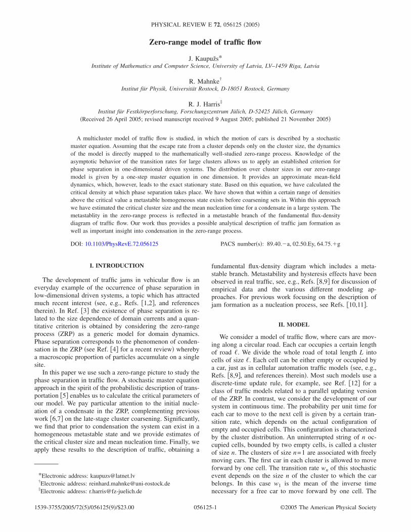
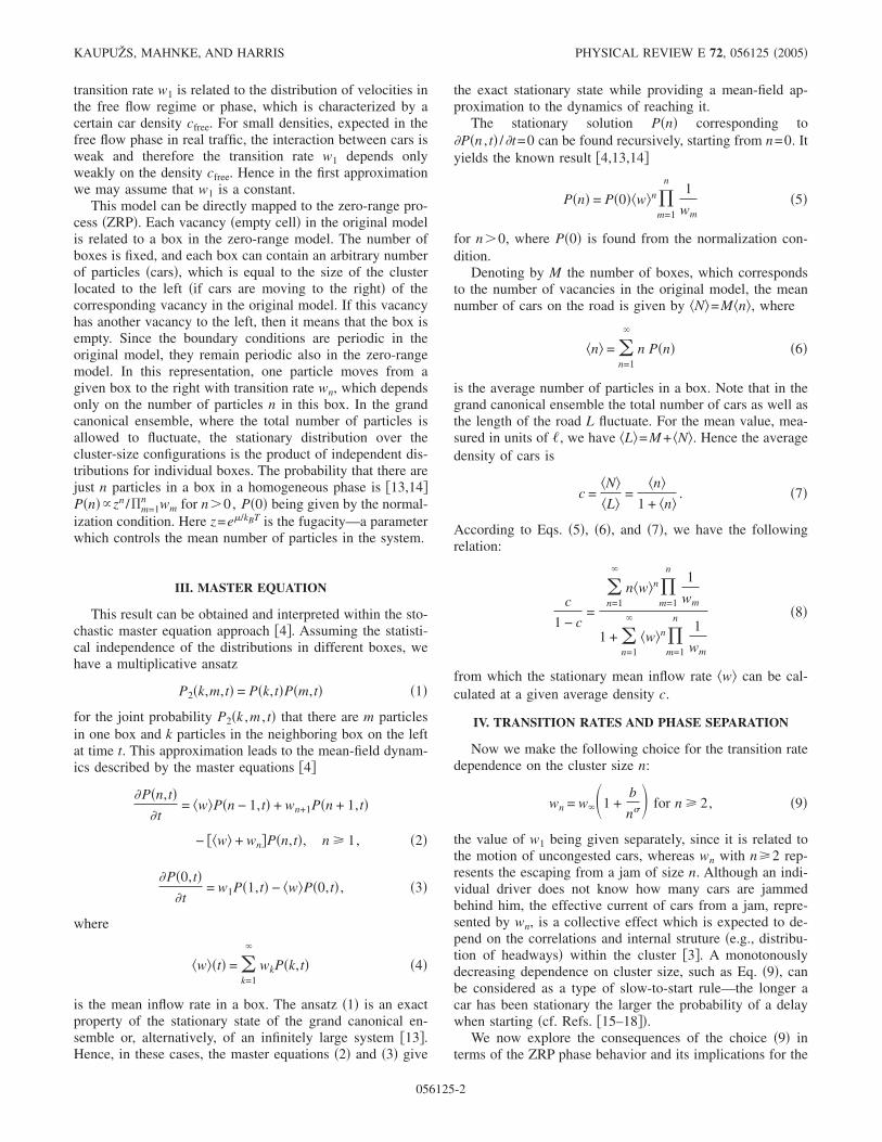
The critical density, calculated numerically from Eqs. �10�and �11� as a function of parameters � and b, is shown inFigs. 2 and 3, respectively. In contrast to the situations dis-cussed previously in the literature, in our model w1 is notgiven by the general formula �9� but is an independent pa-rameter. This distinction leads to quantitatively different re-

FIG. 1. �w� /w� vs density c at b=1 for different �. FIG. 2. Critical density as a function of control parameter � fordifferent values of b.

FIG. 3. Critical density as a function of control parameter b fordifferent values of �.

ZERO-RANGE MODEL OF TRAFFIC FLOW PHYSICAL REVIEW E 72, 056125 �2005�

056125-3

sults, for example, the critical density for �=1 is analyticallyshown to be �22�

ccr =b�b + 1�

�b − 1��2�b + 1� + w1�b − 2��. �12�

V. METASTABILITY

Suppose that at the initial time moment t=0 the system isin a homogeneous state with overall density slightly largerthan ccr. Here we study the development of such a state inthe mean-field approximation provided by Eqs. �2� and �3�.With this initial condition, the mean inflow rate in a box �w�is slightly larger than that at c=ccr , i.e., �w�=w�+� holdswith small and positive �. Hence only large clusters withwn�w�+� have a stable tendency to grow, whereas anysmaller cluster typically �except a rare case� fluctuates until itfinally dissolves. In other words, the initially homogeneoussystem with no large clusters can stay in this metastable su-persaturated state for a long time until a large stable clusterappears due to a rare fluctuation.

Neglecting the fluctuations, the time development of thesize n of a cluster is described by the deterministic equation

dn

dt= �w� − wn. �13�

According to this equation, the undercritical clusters with n�ncr tend to dissolve, whereas the overcritical ones with n�ncr tend to grow, where the critical cluster size ncr is givenby the condition

�w� = wncr. �14�

Using Eq. �9� yields

ncr � b

�w�/w� − 11/�

. �15�

In this case ncr is rounded to an integer value.This deterministic approach describes only the most prob-

able scenario for an arbitrarily chosen cluster of a given size.It does not allow one to obtain the distribution over clustersizes: the deterministic equation �13� suggests that all clus-ters shrink to zero size if they are smaller than ncr at thebeginning, whereas the real size distribution arises from thecompetition between opposite stochastic events of shrinkingand growing. Assuming that the distribution of relativelysmall clusters contributing to �n� is quasistationary, i.e., thatthe detailed balance �equality of the terms in Eqs. �2� and �3�describing opposite stochastic events� for these clusters isalmost reached before any cluster with n�ncr has appeared,we have

�n� � �n=1

ncr

n P�n� �16�

for such a metastable state. In this case from Eq. �7� weobtain

c

1 − c�

�n=1

ncr

n�w�n�m=1

n1

wm

1 + �n=1

ncr

�w�n�m=1

n1

wm

�17�

instead of Eq. �8� for calculation of �w� in this homogeneousmetastable state. The critical cluster size is found self con-sistently solving Eqs. �15� and �17� as a system of equations.From Eq. �15� we see that the critical cluster size ncr divergesat c→ccr , since �w�→w�. The results of calculation of ncr

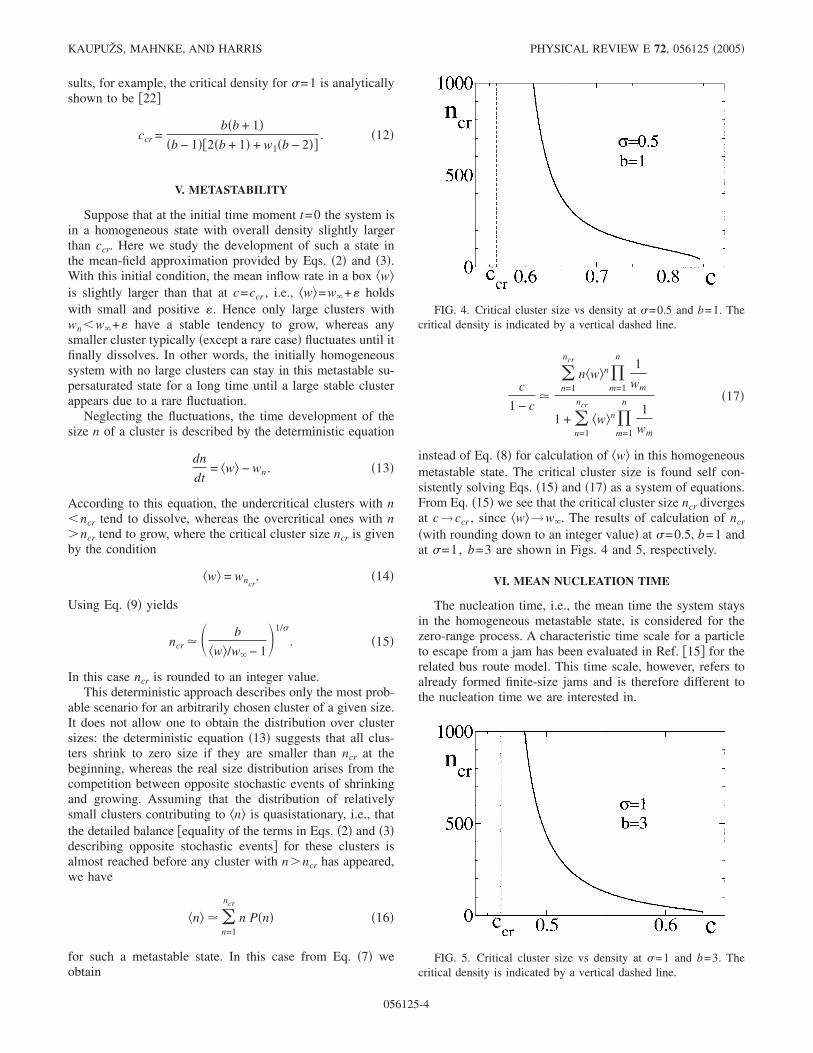
�with rounding down to an integer value� at �=0.5, b=1 andat �=1, b=3 are shown in Figs. 4 and 5, respectively.

VI. MEAN NUCLEATION TIME

The nucleation time, i.e., the mean time the system staysin the homogeneous metastable state, is considered for thezero-range process. A characteristic time scale for a particleto escape from a jam has been evaluated in Ref. �15� for therelated bus route model. This time scale, however, refers toalready formed finite-size jams and is therefore different tothe nucleation time we are interested in.

FIG. 4. Critical cluster size vs density at �=0.5 and b=1. Thecritical density is indicated by a vertical dashed line.

FIG. 5. Critical cluster size vs density at �=1 and b=3. Thecritical density is indicated by a vertical dashed line.


056125-4

Within the framework of mean-field dynamics, the meannucleation time in our model can be evaluated as follows.Let P�t� be the probability density of the first passage time toexceed the critical number of particles ncr in a single box. Byour definition, the nucleation occurs when one of the Mboxes reaches the cluster size ncr+1. The probability that itoccurs first in a given box within a small time interval �t ; t+dt� is thus P�t�dt �1− 0

t P�t��dt��M−1 according to our as-sumption that the boxes are statistically independent. Theterm �1− 0

t P�t��dt��M−1 is the probability that in all otherboxes, except the given one, the overcritical cluster size ncr+1 has still not been reached. Since the nucleation can occurin any of M boxes, the nucleation probability density PM�t�for the system of M boxes is given by

PM�t� = M P�t� �1 − �0

t

P�t��dt��M−1

� MP�t�exp− M�0

t

P�t��dt� . �18�

The latter equality holds for large M, since all M boxes areequivalent, and therefore the probability 0

t P�t��dt� that thenucleation occurs in a given box within a characteristic timeinterval t��T�M is a small quantity of order 1 /M. The meannucleation time for the system of M boxes is

�T�M = �0

�

t PM�t�dt . �19�

Here �T�1 is the mean first passage time for a single box.In order to estimate �T�M according to Eqs. �18� and �19�,

one needs some idea about the first passage time probabilitydensity for one box P�t�. This is actually the problem of aparticle escaping from a potential well. Since we start withan almost homogeneous state of the system, we may assumezero cluster size n=0 as the initial condition. The first pas-sage time probability density can be calculated as the prob-ability per unit time to reach the state ncr+1, assuming thatthe particle is absorbed there. It is reasonable to assume thatafter a certain equilibration time teq, when a quasistationarydistribution of the cluster sizes within nncr is reached, theescaping from this region is characterized by a certain tran-sition rate wesc. Hence for t� teq we have

P�t� � wesc �1 − �0

t

P�t��dt�� , �20�

where the expression in square brackets is the probabilitythat the absorption at ncr+1 has still not occurred up to thetime moment t. At high enough potential barriers �large meanfirst passage times� the short-time contribution to the integralis irrelevant and, by means of Eq. �19�, the solution of Eq.�20� can be written as

P�t� =1

�T�1exp−

t

�T�1 , �21�

where �T�1=wesc−1 . Obviously, this approximate solution of the

first passage problem is not valid for very short times t� teq, since the short-time solution should explicitly dependon the initial condition. In particular, if we start at n=0, thenthe state ncr+1 cannot be reached immediately, so thatP�0�=0. Nevertheless Eq. �21� can be used to estimate themean nucleation time �T�M provided that �T�M � teq.

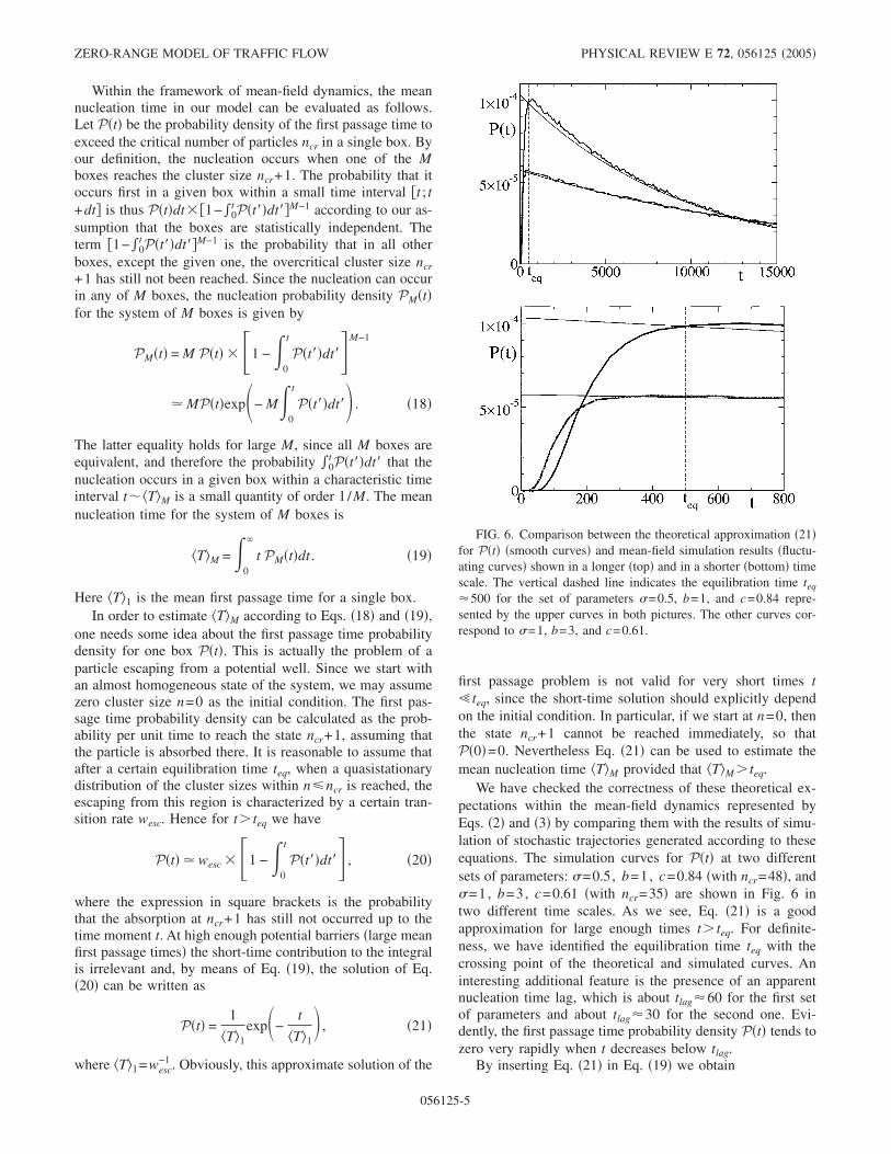
We have checked the correctness of these theoretical ex-pectations within the mean-field dynamics represented byEqs. �2� and �3� by comparing them with the results of simu-lation of stochastic trajectories generated according to theseequations. The simulation curves for P�t� at two differentsets of parameters: �=0.5, b=1, c=0.84 �with ncr=48�, and�=1, b=3, c=0.61 �with ncr=35� are shown in Fig. 6 intwo different time scales. As we see, Eq. �21� is a goodapproximation for large enough times t� teq. For definite-ness, we have identified the equilibration time teq with thecrossing point of the theoretical and simulated curves. Aninteresting additional feature is the presence of an apparentnucleation time lag, which is about tlag�60 for the first setof parameters and about tlag�30 for the second one. Evi-dently, the first passage time probability density P�t� tends tozero very rapidly when t decreases below tlag.

By inserting Eq. �21� in Eq. �19� we obtain

FIG. 6. Comparison between the theoretical approximation �21�for P�t� �smooth curves� and mean-field simulation results �fluctu-ating curves� shown in a longer �top� and in a shorter �bottom� timescale. The vertical dashed line indicates the equilibration time teq

�500 for the set of parameters �=0.5, b=1, and c=0.84 repre-sented by the upper curves in both pictures. The other curves cor-respond to �=1, b=3, and c=0.61.


056125-5

�T�M � M�T�1�0

�

x e−xexp�− M�1 − e−x��dx �22�

after changing the integration variable t / �T�1→x. Takinginto account that only the region x�1/M contributes to theintegral at large M, we arrive at a very simple expression,

�T�M ��T�1

M, �23�

relating the mean first passage time or nucleation time in asystem of M boxes with that of one box. The latter can becalculated easily by the known formula �23�

�T�1 = �n=0

ncr

��w�P̃�n��−1�m=0

n

P̃�m� , �24�

where P̃�0�=1 and P̃�n�=�k=1n ��w� /wk� with n�1 represent

the unnormalized stationary probability distribution.The mean nucleation time versus density c, calculated

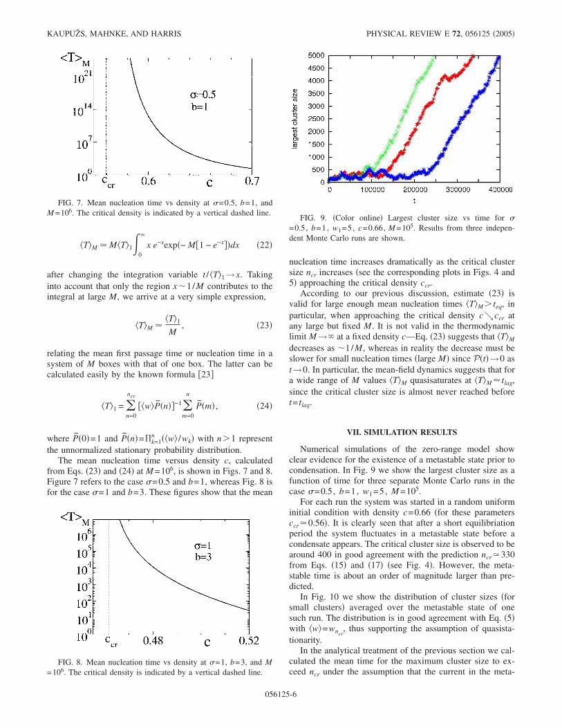
from Eqs. �23� and �24� at M =106, is shown in Figs. 7 and 8.Figure 7 refers to the case �=0.5 and b=1, whereas Fig. 8 isfor the case �=1 and b=3. These figures show that the mean

nucleation time increases dramatically as the critical clustersize ncr increases �see the corresponding plots in Figs. 4 and5� approaching the critical density ccr.

According to our previous discussion, estimate �23� isvalid for large enough mean nucleation times �T�M � teq, inparticular, when approaching the critical density c↘ccr atany large but fixed M. It is not valid in the thermodynamiclimit M→� at a fixed density c—Eq. �23� suggests that �T�M

decreases as �1/M, whereas in reality the decrease must beslower for small nucleation times �large M� since P�t�→0 ast→0. In particular, the mean-field dynamics suggests that fora wide range of M values �T�M quasisaturates at �T�M � tlag,since the critical cluster size is almost never reached beforet= tlag.

VII. SIMULATION RESULTS

Numerical simulations of the zero-range model showclear evidence for the existence of a metastable state prior tocondensation. In Fig. 9 we show the largest cluster size as afunction of time for three separate Monte Carlo runs in thecase �=0.5, b=1, w1=5 , M =105.

For each run the system was started in a random uniforminitial condition with density c=0.66 �for these parametersccr�0.56�. It is clearly seen that after a short equilibriationperiod the system fluctuates in a metastable state before acondensate appears. The critical cluster size is observed to bearound 400 in good agreement with the prediction ncr�330from Eqs. �15� and �17� �see Fig. 4�. However, the meta-stable time is about an order of magnitude larger than pre-dicted.

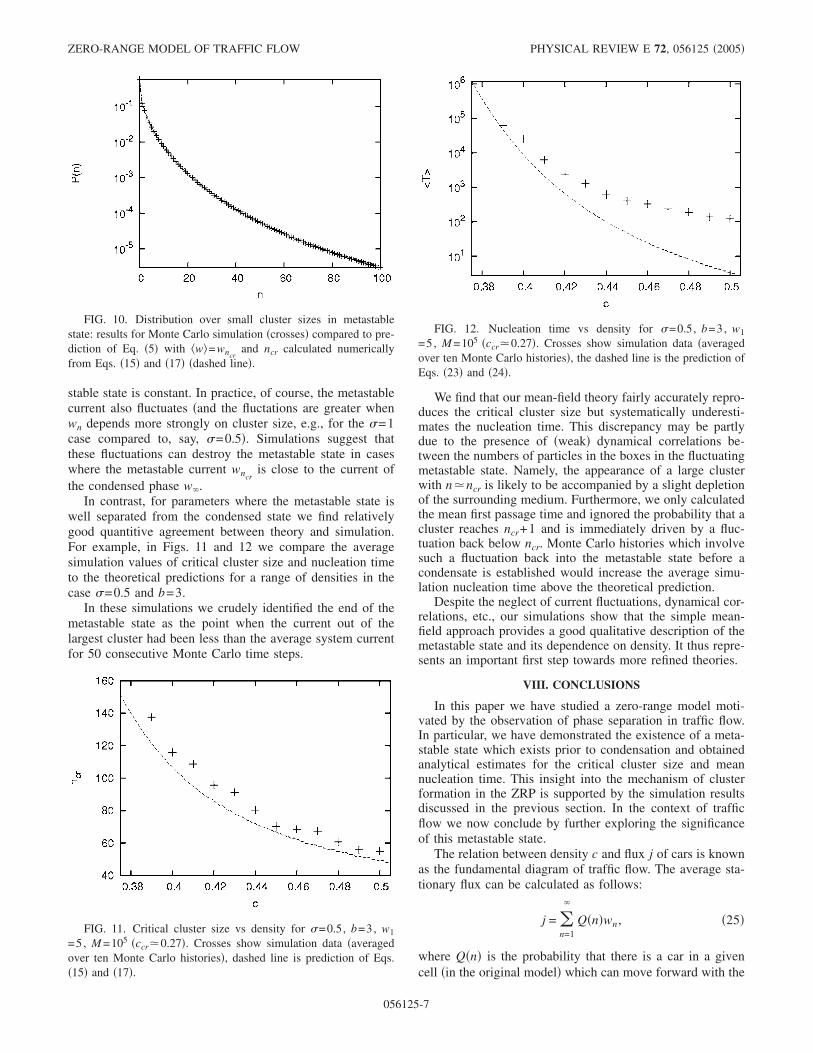
In Fig. 10 we show the distribution of cluster sizes �forsmall clusters� averaged over the metastable state of onesuch run. The distribution is in good agreement with Eq. �5�with �w�=wncr

, thus supporting the assumption of quasista-tionarity.

In the analytical treatment of the previous section we cal-culated the mean time for the maximum cluster size to ex-ceed ncr under the assumption that the current in the meta-

FIG. 8. Mean nucleation time vs density at �=1, b=3, and M=106. The critical density is indicated by a vertical dashed line.

FIG. 9. �Color online� Largest cluster size vs time for �=0.5, b=1, w1=5, c=0.66, M =105. Results from three indepen-dent Monte Carlo runs are shown.

FIG. 7. Mean nucleation time vs density at �=0.5, b=1, andM =106. The critical density is indicated by a vertical dashed line.


056125-6

stable state is constant. In practice, of course, the metastablecurrent also fluctuates �and the fluctations are greater whenwn depends more strongly on cluster size, e.g., for the �=1case compared to, say, �=0.5�. Simulations suggest thatthese fluctuations can destroy the metastable state in caseswhere the metastable current wncr

is close to the current ofthe condensed phase w�.

In contrast, for parameters where the metastable state iswell separated from the condensed state we find relativelygood quantitive agreement between theory and simulation.For example, in Figs. 11 and 12 we compare the averagesimulation values of critical cluster size and nucleation timeto the theoretical predictions for a range of densities in thecase �=0.5 and b=3.

In these simulations we crudely identified the end of themetastable state as the point when the current out of thelargest cluster had been less than the average system currentfor 50 consecutive Monte Carlo time steps.

We find that our mean-field theory fairly accurately repro-duces the critical cluster size but systematically underesti-mates the nucleation time. This discrepancy may be partlydue to the presence of �weak� dynamical correlations be-tween the numbers of particles in the boxes in the fluctuatingmetastable state. Namely, the appearance of a large clusterwith n�ncr is likely to be accompanied by a slight depletionof the surrounding medium. Furthermore, we only calculatedthe mean first passage time and ignored the probability that acluster reaches ncr+1 and is immediately driven by a fluc-tuation back below ncr. Monte Carlo histories which involvesuch a fluctuation back into the metastable state before acondensate is established would increase the average simu-lation nucleation time above the theoretical prediction.

Despite the neglect of current fluctuations, dynamical cor-relations, etc., our simulations show that the simple mean-field approach provides a good qualitative description of themetastable state and its dependence on density. It thus repre-sents an important first step towards more refined theories.

VIII. CONCLUSIONS

In this paper we have studied a zero-range model moti-vated by the observation of phase separation in traffic flow.In particular, we have demonstrated the existence of a meta-stable state which exists prior to condensation and obtainedanalytical estimates for the critical cluster size and meannucleation time. This insight into the mechanism of clusterformation in the ZRP is supported by the simulation resultsdiscussed in the previous section. In the context of trafficflow we now conclude by further exploring the significanceof this metastable state.

The relation between density c and flux j of cars is knownas the fundamental diagram of traffic flow. The average sta-tionary flux can be calculated as follows:

j = �n=1

�

Q�n�wn, �25�

where Q�n� is the probability that there is a car in a givencell �in the original model� which can move forward with the

FIG. 10. Distribution over small cluster sizes in metastablestate: results for Monte Carlo simulation �crosses� compared to pre-diction of Eq. �5� with �w�=wncr

and ncr calculated numericallyfrom Eqs. �15� and �17� �dashed line�.

FIG. 11. Critical cluster size vs density for �=0.5, b=3, w1

=5, M =105 �ccr�0.27�. Crosses show simulation data �averagedover ten Monte Carlo histories�, dashed line is prediction of Eqs.�15� and �17�.

FIG. 12. Nucleation time vs density for �=0.5, b=3, w1

=5, M =105 �ccr�0.27�. Crosses show simulation data �averagedover ten Monte Carlo histories�, the dashed line is the prediction ofEqs. �23� and �24�.


056125-7

rate wn. Note that only those cars contribute to the flux,which are the first in some cluster. Hence Q�n�=�P�n� /�m=1

� P�m�, where � is the fraction of cells, whichcontain such cars. This fraction can be calculated easily asthe number of clusters divided by the total number of cells.These quantities fluctuate in our model. For large systems,however, they can be replaced by the mean values. The meannumber of clusters is equal to the mean number of nonemptyboxes M�n=1

� P�n� in the zero-range model, whereas themean number of cells, i.e., the mean length of the road is�L�=M + �N�=M�1+ �n��=M / �1−c�, as we have already dis-cussed in Sec. III. Hence Q�n�= �1−c�P�n� and Eq. �25� re-duces to

j = �1 − c��w� . �26�

The mean stationary transition rate �w� depends on the cardensity c. For undercritical densities c�ccr, this quantity isthe solution of Eq. �8�. For overcritical densities we have�w�=w� in the phase coexistence regime, as discussed inSec. IV, therefore in this case the fundamental diagram re-duces to a straight line

j = �1 − c�w�, c � ccr. �27�

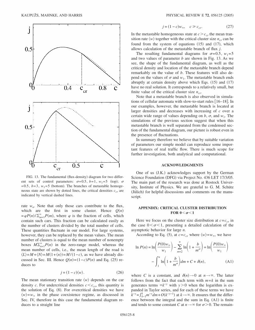
In the metastable homogeneous state at c�ccr the mean tran-sition rate �w� together with the critical cluster size ncr can befound from the system of equations �15� and �17�, whichallows calculation of the metastable branch of flux j.

The resulting fundamental diagrams for �=0.5, w1=5and two values of parameter b are shown in Fig. 13. As wesee, the shape of the fundamental diagram, as well as thecritical density and location of the metastable branch dependremarkably on the value of b. These features will also de-pend on the values of � and w1. The metastable branch endsabruptly at certain density above which Eqs. �15� and �17�have no real solution. It corresponds to a relatively small, butfinite value of the critical cluster size ncr.

Note that a metastable branch is also observed in simula-tions of cellular automata with slow-to-start rules �16–18�. Inour examples, however, the metastable branch is located atlarger densities and decreases with increasing of c over acertain wide range of values depending on b, �, and w1. Thesimulations of the previous section suggest that when thismetastable branch is well separated from the condensed sec-tion of the fundamental diagram, our picture is robust even inthe presence of fluctuations.

In summary therefore we believe that by suitable variationof parameters our simple model can reproduce some impor-tant features of real traffic flow. There is much scope forfurther investigation, both analytical and computational.

ACKNOWLEDGMENTS

One of us �J.K.� acknowledges support by the GermanScience Foundation �DFG� via Project No. 436 LET 17/3/05.The main part of the research was done at Rostock Univer-sity, Institute of Physics. We are grateful to G. M. Schütz�Jülich� for helpful discussions and comments on the manu-script.

APPENDIX: CRITICAL CLUSTER DISTRIBUTIONFOR 0��1

Here we focus on the cluster size distribution at c=ccr inthe case 0��1, presenting a detailed calculation of theasymptotic behavior for large n.

According to Eq. �5�, at c=ccr where �w�=w�, we have

ln P�n� = lnP�0�w�

w1 − �

m=2

n

ln1 +b

m� = lnP�0�w�

w1

− �1

n

ln1 +b

m�dm + C + ��n� , �A1�

where C is a constant, and ��n�→0 at n→�. The latterfollows from the fact that each term with m=k in the sumgenerates terms �k−y with y�0 when the logarithm is ex-panded in Taylor series, and for each of these terms we havek−y = k−1

k m−ydm+O�k−y−1� at k→�. It ensures that the differ-ence between the integral and the sum in Eq. �A1� is finiteand tends to some constant C at n→� for ��0. The remain-

FIG. 13. The fundamental �flux-density� diagram for two differ-ent sets of control parameters: �=0.5, b=1, w1=5 �top�; �=0.5, b=3, w1=5 �bottom�. The branches of metastable homoge-neous state are shown by dotted lines, the critical densities ccr areindicated by vertical dashed lines.


056125-8

der term ��n� is irrelevant for the leading asymptotic behav-ior of P�n�. By expanding the logarithm and integrating termby term, for 0��1 and �� 1

2 , 13 , 1

4 ,… we obtain

P�n� � �k=1

�1/��

exp� �− b�k

k

n1−k�

1 − k�� , �A2�

where �1/�� denotes the integer part of 1 /�. The caseswhere � is an inverse integer are special, since a term �1/mappears in the expansion of the logarithm, giving rise to apowerlike correction to the stretched exponential behavior,viz.

P�n� � n��− b�1/� �k=1

�−1−1

exp� �− b�k

k

n1−k�

1 − k�� A3�

for �= 12 , 1

3 , 14 ,… . The known result for �=1 can also be

obtained by this method: it corresponds to the power-likeprefactor in Eq. �A3�. Only the linear expansion term of thelogarithm is relevant at 1 /2��1, so we find P�n��exp�−b n1−� / �1−�� in the limit of large n. The first twoterms are relevant for 1 /3��1/2, the third one becomesimportant for 1 /4��1/3, and so on. Equations �A2� and�A3� represent an exact analytical result at n→� which wehave also verified numerically at different values of � and b.In this form, where the proportionality coefficient is notspecified, Eqs. �A2� and �A3� are universal, i.e., they do notdepend on the choice of w1.

�1� D. Mukamel, in Soft and Fragile Matter: Nonequilibrium Dy-namics, Metastability and Flow, edited by M. E. Cates and M.R. Evans �Institute of Physics Publishing, Bristol, 2000�.

�2� G. M. Schütz, J. Phys. A 36, R339 �2003�.�3� Y. Kafri, E. Levine, D. Mukamel, G. M. Schütz, and J. Török,

Phys. Rev. Lett. 89, 035702 �2002�.�4� M. R. Evans and T. Hanney, J. Phys. A 38, R195 �2005�.�5� R. Mahnke, J. Kaupužs, and I. Lubashevsky, Phys. Rep. 408,

1 �2005�.�6� S. Grosskinsky, G. M. Schütz, and H. Spohn, J. Stat. Phys.

113, 389 �2003�.�7� C. Godrèche, J. Phys. A 36, 6313 �2003�.�8� D. Chowdhury, L. Santen, and A. Schadschneider, Phys. Rep.

329, 199 �2000�.�9� D. Helbing, Rev. Mod. Phys. 73, 1067 �2001�.

�10� R. Mahnke and J. Kaupužs, Phys. Rev. E 59, 117 �1999�.�11� R. Mahnke, J. Kaupužs, and V. Frishfelds, Atmos. Res. 65,

261 �2003�.�12� E. Levine, G. Ziv, L. Gray, and D. Mukamel, Physica A 340,

636 �2004�.�13� F. Spitzer, Adv. Math. 5, 246 �1970�.�14� M. R. Evans, Braz. J. Phys. 30, 42 �2000�.�15� O. J. O’Loan, M. R. Evans, and M. E. Cates, Phys. Rev. E 58,

1404 �1998�.�16� M. Takayasu and H. Takayasu, Fractals 1, 860 �1993�.�17� S. C. Benjamin, N. F. Johnson, and P. M. Hui, J. Phys. A 29,

3119 �1996�.�18� R. Barlovic, L. Santen, A. Schadschneider, and M. Schrecken-

berg, Eur. Phys. J. B 5, 793 �1998�.�19� J. Kaupužs and R. Mahnke, Eur. Phys. J. B 14, 793 �2000�.�20� Y. Kafri, E. Levine, D. Mukamel, G. M. Schütz, and R. D.

Willmann, Phys. Rev. E 68, 035101�R� �2003�.�21� I. Jeon, P. March, Can. Math. Soc. Conf. Proc. 26, 233 �2000�.�22� G. M. Schütz �private communication�.�23� C. W. Gardiner, Handbook of Stochastic Methods for Physics,

Chemistry, and the Natural Sciences �Springer, Berlin, 1983,1994�.


056125-9

Documents

Zero-range model of traffic flow