ZEROS OF ORTHOGONAL POLYNOMIALS GENERATED · ZEROS OF ORTHOGONAL POLYNOMIALS GENERATED ... (x−c) dµ(x)+Nδ ... sharp bounds and speed of convergence to them for their

Pre-Publicacoes do Departamento de MatematicaUniversidade de CoimbraPreprint Number 14–07

ZEROS OF ORTHOGONAL POLYNOMIALS GENERATEDBY THE GERONIMUS PERTURBATION OF MEASURES

AMILCAR BRANQUINHO, EDMUNDO J. HUERTAS AND FERNANDO R. RAFAELI

Abstract: This paper deals with monic orthogonal polynomial sequences (MOPSin short) generated by a Geronimus canonical spectral transformation of a positiveBorel measure µ, i.e.,

1

(x− c)dµ(x) +Nδ(x− c),

for some free parameter N ∈ R+ and shift c. We analyze the behavior of thecorresponding MOPS. In particular, we obtain such a behavior when the mass N

tends to infinity as well as we characterize the precise values of N such the smallest(respectively, the largest) zero of these MOPS is located outside the support of theoriginal measure µ. When µ is semi-classical, we obtain the ladder operators andthe second order linear differential equation satisfied by the Geronimus perturbedMOPS, and we also give an electrostatic interpretation of the zero distribution interms of a logarithmic potential interaction under the action of an external field.We analyze such an equilibrium problem when the mass point of the perturbationc is located outside the support of µ.

Keywords: Orthogonal polynomials, Canonical spectral transformations of mea-sures, Zeros, Interlacing, Monotonicity, Laguerre and Jacobi polynomials, Asymp-totic behavior, Electrostatic interpretation, Logarithmic potential.AMS Subject Classification (2000): 30C15.

1. Introduction

1.1. Geronimus perturbation of a measure. In the last years someattention has been paid to the so called canonical spectral transformationsof measures. Some authors have analyzed them from the point of view ofStieltjes functions associated with such a kind of perturbations (see [27]) or

Received February 25, 2014.The work of the first author was partially supported by Centro de Matematica da Universidade

de Coimbra (CMUC), funded by the European Regional Development Fund through the programCOMPETE and by the Portuguese Government through the FCT - Fundacao para a Ciencia e aTecnologia under the project PEst-C/MAT/UI0324/2011.

The work of the second author was supported by Fundacao para a Ciencia e a Tecnologia(FCT) of Portugal, ref. SFRH/BPD/91841/2012, and partially supported by Direccion Generalde Investigacion Cientıfica y Tecnica, Ministerio de Economıa y Competitividad of Spain, grantMTM2012-36732-C03-01.

The third author wishes to thank FAPESP and CNPq for their financial support.

1

2 A. BRANQUINHO, E. J. HUERTAS AND F. R. RAFAELI

from the relation between the corresponding Jacobi matrices (see [28]). Thepresent contribution is focused on the behavior of zeros of monic orthogonalpolynomial sequences (MOPS in the sequel) associated with a particulartransformation of measures called the Geronimus canonical transformationon the real line. Let µ be an absolutely continuous measure with respect tothe Lebesgue measure supported on a finite or infinite interval E = supp(µ),such that C0(E) = [a, b] ⊆ R. The basic Geronimus perturbation of µ isdefined as

dνN(x) =1

(x− c)dµ(x) +Nδ(x− c), (1)

with N ∈ R+, δ(x − c) the Dirac delta function in x = c, and the shift ofthe perturbation verifies c 6∈ E. Observe that it is given simultaneously by arational modification of µ by a positive linear polynomial whose real zero cis the point of transformation (also known as the shift of the transformation)and the addition of a Dirac mass at the point of transformation as well.This transformation was introduced by Geronimus in the seminal papers

[11] and [12] devoted to provide a procedure of constructing new families oforthogonal polynomials from other orthogonal families, and also was studiedby Shohat (see [22]) concerning about mechanical quadratures. The problemwas revisited by Maroni in [19], into a more general algebraic frame, whogives an expression for the MOPS associated with (1) in terms of the socalled co-recursive polynomials of the classical orthogonal polynomials. Inthe past decade, Bueno and Marcellan reinterpreted this perturbation in theframework of the so called discrete Darboux transformations, LU and ULfactorizations of shifted Jacobi matrices [5]. This interpretation as Darbouxtransformations, together with other canonical transformations (Christoffeland Uvarov), provide a link between orthogonal polynomials and discreteintegrable systems (see [1], [23] and [24]). More recently, in [4] the authorspresent a new computational algorithm for computing the Geronimus trans-formation with large shifts, and [7] concerns about a new revision of theGeronimus transformation in terms of symmetric bilinear forms in order toinclude certain Sobolev and Sobolev–type orthogonal polynomials into thescheme of Darboux transformations.In order to justify the relevance of this contribution, we point out that

the behavior of the zeros of orthogonal polynomials is extensively studiedbecause of their applications in many areas of mathematics, physics and en-gineering. Following this premise, the purpose of this paper is twofold. First,

ZEROS OF GERONIMUS PERTURBED ORTHOGONAL POLYNOMIALS 3

using a similar approach as was done in [14], we provide a new connectionformula for the Geronimus perturbed MOPS, which will be crucial to obtainsharp limits (and the speed of convergence to them) of their zeros. We pro-vide a comprehensive study of the zeros in terms of the free parameter ofthe perturbation N , which somehow determines how important the pertur-bation on the classical measure µ is. Notice that this work also concerns withthe behavior of the eigenvalues of the monic Jacobi matrices associated tocertain Darboux transformations with shift c and free parameter N studiedin [4]. Second, from the aforementioned new connection formula we recover(from an alternative point of view) a connection formula already known inthe literature (see [19]) in terms of two consecutive polynomials of the origi-nal measure µ. We also obtain explicit expressions for the ladder operatorsand the second order differential equation satisfied by the Geronimus per-turbed MOPS. When the measure µ is semi-classical, we also obtain thecorresponding electrostatic model for the zeros of the Geronimus perturbedMOPS, showing that they are the electrostatic equilibrium points of positiveunit charges interacting according to a logarithmic potential under the actionof an external field (see, for example, Szego’s book [25, Section 6.7], Ismail’sbook [17, Ch. 3] and the references therein).The structure of the paper is as follows. The rest of this Section is devoted

to introduce without proofs some relevant material about modified innerproducts and their corresponding MOPS. In Section 2 we provide our mainresults. We obtain a new connection formula for orthogonal polynomials ge-nerated by a basic Geronimus transformation of a positive Borel measure µ,sharp bounds and speed of convergence to them for their real zeros, and theladder operators and the second linear differential equation that they satisfy.The results about the zeros follows from a lemma concerning the behavior ofthe zeros of a linear combination of two polynomials. In Section 3, we proofall the result provided in the former Section. Finally, in Section 4, we ex-plore these results for the Geronimus perturbed Laguerre and Jacobi MOPS.For µ being semi-classical, we obtain the corresponding electrostatic modelfor the zeros of the Geronimus perturbed MOPS as equilibrium points in alogarithmic potential interaction of positive unit charges under the presenceof an external field. We analyze such an equilibrium problem when the masspoint is located outside the support of the measure µ, and we provide explicitformulas for the Laguerre and Jacobi weight cases.


1.2. Modified inner products and notation. Let µ be a positive Borelmeasure µ, with existing moments of all orders, and supported on a subsetE ⊆ R with infinitely many points. Given such a measure, we define thestandard inner product 〈·, ·〉µ : P× P → R by

〈f, g〉µ =

∫

E

f(x)g(x)dµ(x), f, g ∈ P, (2)

where P is the linear space of the polynomials with real coefficients, and thecorresponding norm || · ||µ : P → [0,+∞) is given, as usual, by

||f ||µ =

√

∫

E

|f(x)|2dµ(x), f ∈ P.

Let {Pn}n≥0 be the MOPS associated with µ. It is very well known that theformer MOPS satisfy the three term recurrence relation

xPn(x) = Pn+1(x) + βnPn(x) + γnPn−1(x), (3)

P−1(x) = 0, P0(x) = 1.

If

Kn(x, y) =n

∑

k=0

Pk(x)Pk(y)

||Pk||2µ(4)

denotes the corresponding n-th kernel polynomial, according to the Christoffel-Darboux formula, for every n ∈ N we have

Kn(x, y) =Pn+1(x)Pn(y)− Pn+1(y)Pn(x)

(x− y)

1

||Pn||2µ.

Notice that this structures satisfy the well-known “reproducing property” ofthe n-th kernel polynomial

∫

E

Kn (x, y) f (x) dµ(x) = f (y)

for any polynomial f ∈ P with deg (f) ≤ n.

Here and subsequently, {Pc,[k]n }n≥0 denotes the MOPS with respect to the

modified inner product

〈f, g〉µ,[k] =

∫

E

f(x)g(x)(x− c)kdµ(x), (5)

where c /∈ E = supp(µ). The polynomials {Pc,[k]n }n≥0 are orthogonal with

respect to a polynomial modification of the measure µ called the k-iterated


Christoffel perturbation. If k = 1 we have the Christoffel canonical transfor-

mation of the measure µ (see [27] and [28]). It is well known that Pc,[1]n (x) is

the monic kernel polynomial which can be represented as (see [6, (7.3)])

P c,[1]n (x) =

1

(x− c)(Pn+1(x)− πn Pn(x)) =

‖Pn‖2µ

Pn(c)Kn(x, c), (6)

with

πn = πn(c) =Pn+1(c)

Pn(c). (7)

Notice that Pc,[1]n (c) 6= 0. We will denote

||P c,[k]n ||2µ,[k] =

∫

E

|P c,[k]n (x)|2(x− c)kdµ.

Next, let us consider the basic Geronimus perturbation of µ given in (1).Let {Qc

n}n≥0 be the MOPS associated with dνN(x) when the N = 0. Thatis, they are orthogonal with respect to the measure

dνN=0(x) = dν(x) =1

(x− c)dµ(x). (8)

This constitutes a linear rational modification of µ, and the correspondingMOPS {Qc

n}n≥0 with respect to

〈f, g〉ν =

∫

E

f(x)g(x)dν(x) =

∫

E

f(x)g(x)1

(x− c)dµ(x) (9)

has been extensively studied in the literature (see, among others, [3], [10,2.4.2], [17, 2.7], [26], and [27]). It is also well known that Qc

n(x) can berepresented as

Qcn(x) = Pn(x)− rn−1 Pn−1(x), n = 0, 1, 2, . . . , (10)

where Qc0(x) = 1,

rn−1 = rn−1(c) =Fn(c)

Fn−1(c), c /∈ E, (11)

and F−1(c) = 1. The functions

Fn(s) =

∫

E

Pn(x)

x− sdµ(x), s ∈ C\E,


are the Cauchy integrals of {Pn}n≥0, or functions of the second kind associa-ted with the monic polynomials {Pn}n≥0. For a proper way to compute theabove Cauchy integrals, we refer the reader to [10, 2.3].It is clear that

Kcn(x, y) =

n∑

k=0

Qck(x)Q

ck(y)

||Qck||

2ν

=Qc

n+1(x)Qcn(y)−Qc

n+1(y)Qcn(x)

(x− y)

1

||Qcn||

2ν

(12)

are the kernel polynomials corresponding to the MOPS {Qcn}n≥0, which also

satisfies the corresponding reproducing property of polynomial kernels withrespect to the measure dν

∫

E

f (x)Kcn (x, c) dν(x) = f (c) , (13)

for any polynomial f ∈ P with deg f ≤ n. The so called confluent form of(12) is given by (see [6])

Kcn(c, c) =

[Qcn+1]

′(c)Qcn(c)− [Qc

n]′(c)Qc

n+1(c)

||Qcn||

2ν

, (14)

which is always a positive quantity

Kcn(c, c) =

n∑

k=0

[Qck(c)]

2

‖Qck‖

2ν

> 0. (15)

The key concept to find several of our results is that the polynomials {Pn}n≥0

are the monic kernel polynomials of parameter c of the sequence {Qcn}n≥0.

According to this argument, the following expressions

Pn(x) =‖Qc

n‖2ν

Qcn(c)

Kcn(x, c) =

1

(x− c)

(

Qcn+1(x)−

Qcn+1(c)

Qcn(c)

Qcn(x)

)

(16)

hold.Finally, let {Qc,N

n }n≥0 be the MOPS associated to dνN when N > 0. That

is, {Qc,Nn }n≥0 are the Geronimus perturbed polynomials orthogonal with res-

pect to the the inner product

〈f, g〉νN =

∫

E

f(x)g(x)1

(x− c)dµ(x) +Nf(c)g(c). (17)

Note that this is a standard inner product in the sense that, for every f, g ∈ P,we have 〈xf, g〉νN = 〈f, xg〉νN . From (9) and (17), a trivial verification shows


that〈f, g〉νN = 〈f, g〉ν +Nf(c)g(c). (18)

Is the aim of this contribution to find and analyze the asymptotic behaviorof the zeros of Qc,N

n (x) with the parameter N , present in the Geronimus per-turbation (1), and provide as well an electrostatic model for these zeros whenthe original measure µ is semiclassical. To this end, we will use some remar-kable facts, which are straightforward consequences of the inner products (2),(5), (9) and (17). Taking into account that the multiplication operator by(x − c) is a symmetric operator with respect to (9), for any f(x), g(x) ∈ P

we have〈(x− c)f, g〉ν = 〈f, (x− c)g〉ν = 〈f, g〉µ

If we consider the polynomials (x − c)f(x) or (x − c)g(x) in the above ex-pression, we deduce

(x− c)f(x)|x=c = (x− c)g(x)|x=c = 0,

which makes it obvious that (x−c) is also a symmetric operator with respectto the Geronimus inner product (17), i.e.,

〈(x− c)f, g〉νN = 〈f, (x− c)g〉νN = 〈(x− c)f, g〉ν. (19)

Finally, another useful consequence of the above relations is

〈(x− c)f, (x− c)g〉νN = 〈f, g〉c,[1]. (20)

2. Statement of the main results

2.1. Connection formulas. Next, we provide a new connection formula forthe Geronimus perturbed orthogonal polynomials Qc,N

n (x), in terms of the

polynomials Qcn(x) and the monic Kernel polynomials P

c,[1]n (x). This repre-

sentation will allow us to obtain the results about monotonicity, asymptotics,and speed of convergence (presented below in this Section) for the zeros ofQc,N

n (x) in terms of the parameter N present in the perturbation (1).

Theorem 1 (connection formula). The MOPS {Qc,Nn }n≥0 can be represented

asQc,N

n (x) = Qcn(x) +NBc

n(x− c)Pc,[1]n−1(x), (21)

with Qc,Nn (x) = κnQ

c,Nn (x), κn = 1 +NBc

n and

Bcn =

−Qcn(c)Pn−1(c)

‖Pn−1‖2µ= Kc

n−1(c, c) > 0. (22)


Observe that one can even give another alternative expression for Bcn, which

only involves polynomials and functions of the second kind relative to theoriginal measure µ, evaluated at the point of tranformation c. Combining(10) with (22), we deduce that

Bcn = Kc

n−1(c, c) =rn−1 P

2n−1 − Pn(c)Pn−1(c)

‖Pn−1‖2µ. (23)

As a direct consequence of the above theorem, we can express Qc,Nn (x) in

terms of only two consecutive elements of the initial sequence {Pn}n≥0. Thisexpression of Qc,N

n (x) was already studied in the literature (see [19, formula(1.4)] and [7, Sec. 1]). In fact, the original aim of Geronimus in its pioneerworks on the subject was to find necessary and sufficient conditions for theexistence of a sequence of coefficients Λn, such that the linear combinationof monic polinomials

Pn(x) + ΛnPn−1(x), Λn 6= 0, n = 1, 2, . . . ,

were, in turn, orthogonal with respect to some measure supported on R. Herewe rewrite the value of Λn in several new equivalent ways. Substituting (10)and (6) into (21) yields

Qc,Nn (x) = κnQ

c,Nn (x) = Pn(x)− rn−1Pn−1(x) +NBc

n (Pn(x)− πn−1Pn−1(x)) .

Thus, having in mind that κn = 1 + NBcn, after some trivial computations

we can state the following result.

Proposition 1. The monic Geronimus perturbed orthogonal polynomials ofthe sequence {Qc,N

n }n≥0 can be represented as

Qc,Nn (x) = Pn(x) + Λc

n Pn−1(x), (24)

with

Λcn = Λc

n(N) =πn−1 − rn−1

1 +NBcn

− πn−1, (25)

and πn−1, rn−1 given respectively in (7) and (11) respectively. Notice that Λcn

is independent of the variable x.

Remark 1. The coefficient Λcn(N) can also be expressed only in terms of

quantities relative to the original non-perturbed measure µ, the point of trans-formation c and the mass N . Thus, from (23) and (25), we obtain

Λcn(N) =

(

1

πn−1 − rn−1−N

P 2n−1(c)

‖Pn−1‖2µ

)−1

− πn−1.


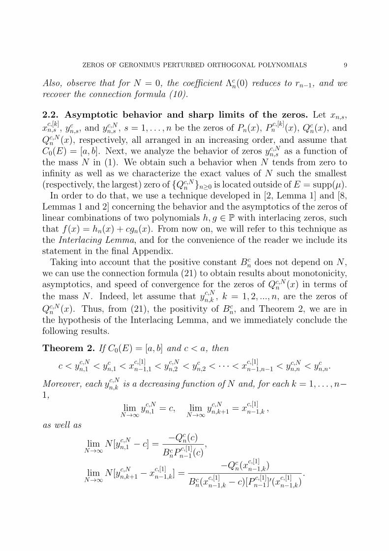
Also, observe that for N = 0, the coefficient Λcn(0) reduces to rn−1, and we

recover the connection formula (10).

2.2. Asymptotic behavior and sharp limits of the zeros. Let xn,s,

xc,[k]n,s , ycn,s, and yc,Nn,s , s = 1, . . . , n be the zeros of Pn(x), P

c,[k]n (x), Qc

n(x), and

Qc,Nn (x), respectively, all arranged in an increasing order, and assume that

C0(E) = [a, b]. Next, we analyze the behavior of zeros yc,Nn,s as a function ofthe mass N in (1). We obtain such a behavior when N tends from zero toinfinity as well as we characterize the exact values of N such the smallest(respectively, the largest) zero of {Qc,N

n }n≥0 is located outside of E = supp(µ).In order to do that, we use a technique developed in [2, Lemma 1] and [8,

Lemmas 1 and 2] concerning the behavior and the asymptotics of the zeros oflinear combinations of two polynomials h, g ∈ P with interlacing zeros, suchthat f(x) = hn(x) + cgn(x). From now on, we will refer to this technique asthe Interlacing Lemma, and for the convenience of the reader we include itsstatement in the final Appendix.Taking into account that the positive constant Bc

n does not depend on N ,we can use the connection formula (21) to obtain results about monotonicity,asymptotics, and speed of convergence for the zeros of Qc,N

n (x) in terms of

the mass N . Indeed, let assume that yc,Nn,k , k = 1, 2, ..., n, are the zeros of

Qc,Nn (x). Thus, from (21), the positivity of Bc

n, and Theorem 2, we are inthe hypothesis of the Interlacing Lemma, and we immediately conclude thefollowing results.

Theorem 2. If C0(E) = [a, b] and c < a, then

c < yc,Nn,1 < ycn,1 < xc,[1]n−1,1 < yc,Nn,2 < ycn,2 < · · · < x

c,[1]n−1,n−1 < yc,Nn,n < ycn,n.

Moreover, each yc,Nn,k is a decreasing function of N and, for each k = 1, . . . , n−1,

limN→∞

yc,Nn,1 = c, limN→∞

yc,Nn,k+1 = xc,[1]n−1,k ,

as well as

limN→∞

N [yc,Nn,1 − c] =−Qc

n(c)

BcnP

c,[1]n−1(c)

,

limN→∞

N [yc,Nn,k+1 − xc,[1]n−1,k] =

−Qcn(x

c,[1]n−1,k)

Bcn(x

c,[1]n−1,k − c)[P

c,[1]n−1 ]

′(xc,[1]n−1,k)

.


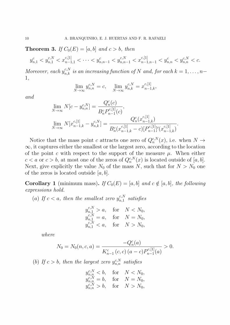
Theorem 3. If C0(E) = [a, b] and c > b, then

ycn,1 < yc,Nn,1 < xc,[1]n−1,1 < · · · < ycn,n−1 < yc,Nn,n−1 < x

c,[1]n−1,n−1 < ycn,n < yc,Nn,n < c.

Moreover, each yc,Nn,k is an increasing function of N and, for each k = 1, . . . , n−1,

limN→∞

yc,Nn,n = c, limN→∞

yc,Nn,k = xc,[1]n−1,k,

and

limN→∞

N [c− yc,Nn,n ] =Qc

n(c)

BcnP

c,[1]n−1(c)

,

limN→∞

N [xc,[1]n−1,k − yc,Nn,k ] =

Qcn(x

c,[1]n−1,k)

Bcn(x

c,[1]n−1,k − c)[P

c,[1]n−1 ]

′(xc,[1]n−1,k)

.

Notice that the mass point c attracts one zero of Qc,Nn (x), i.e. when N →

∞, it captures either the smallest or the largest zero, according to the locationof the point c with respect to the support of the measure µ. When eitherc < a or c > b, at most one of the zeros of Qc,N

n (x) is located outside of [a, b].Next, give explicitly the value N0 of the mass N , such that for N > N0 oneof the zeros is located outside [a, b].

Corollary 1 (minimum mass). If C0(E) = [a, b] and c /∈ [a, b], the followingexpressions hold.

(a) If c < a, then the smallest zero yc,Nn,1 satisfies

yc,Nn,1 > a, for N < N0,

yc,Nn,1 = a, for N = N0,

yc,Nn,1 < a, for N > N0,

where

N0 = N0(n, c, a) =−Qc

n(a)

Kcn−1 (c, c) (a− c)P

c,[1]n−1(a)

> 0.

(b) If c > b, then the largest zero yc,Nn,n satisfies

yc,Nn,n < b, for N < N0,yc,Nn,n = b, for N = N0,yc,Nn,n > b, for N > N0,


where

N0 = N0(n, c, b) =−Qc

n(b)

Kcn−1 (c, c) (b− c)P

c,[1]n−1(b)

> 0.

Proof : (a) In order to deduce the location of yc,Nn,1 with respect to the point

x = a, it is enough to observe that Qc,Nn (a) = 0 if and only if N = N0.

(b) Also, in order to find the location of yc,Nn,n with respect to the point

x = b, notice that Qc,Nn (b) = 0 if and only if N = N0.

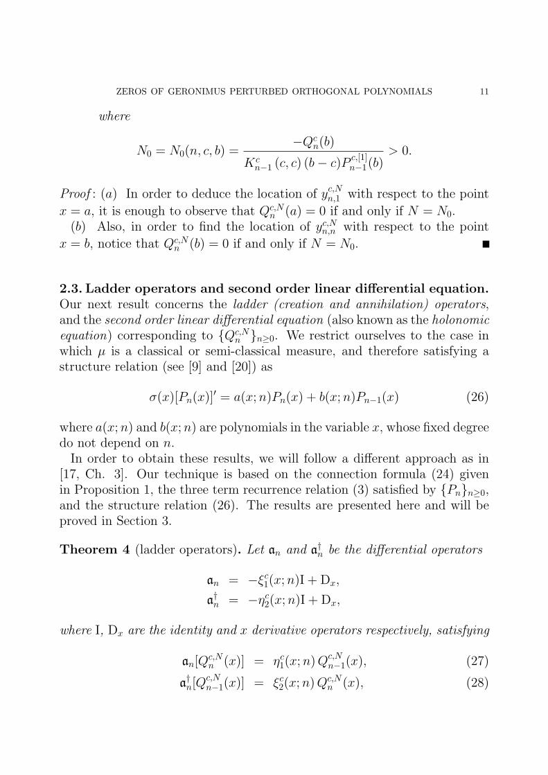
2.3. Ladder operators and second order linear differential equation.

Our next result concerns the ladder (creation and annihilation) operators,and the second order linear differential equation (also known as the holonomicequation) corresponding to {Qc,N

n }n≥0. We restrict ourselves to the case inwhich µ is a classical or semi-classical measure, and therefore satisfying astructure relation (see [9] and [20]) as

σ(x)[Pn(x)]′ = a(x;n)Pn(x) + b(x;n)Pn−1(x) (26)

where a(x;n) and b(x;n) are polynomials in the variable x, whose fixed degreedo not depend on n.In order to obtain these results, we will follow a different approach as in

[17, Ch. 3]. Our technique is based on the connection formula (24) givenin Proposition 1, the three term recurrence relation (3) satisfied by {Pn}n≥0,and the structure relation (26). The results are presented here and will beproved in Section 3.

Theorem 4 (ladder operators). Let an and a†n be the differential operators

an = −ξc1(x;n)I + Dx,

a†n = −ηc2(x;n)I + Dx,

where I, Dx are the identity and x derivative operators respectively, satisfying

an[Qc,Nn (x)] = ηc1(x;n)Q

c,Nn−1(x), (27)

a†n[Q

c,Nn−1(x)] = ξc2(x;n)Q

c,Nn (x), (28)


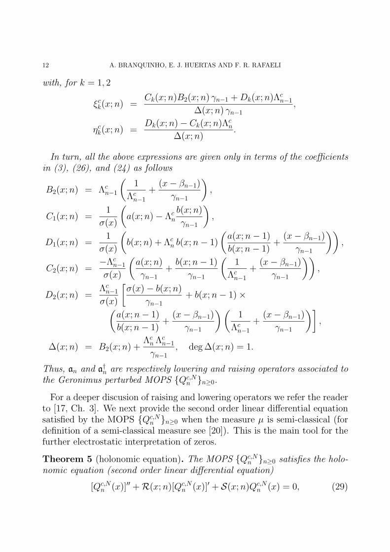
with, for k = 1, 2

ξck(x;n) =Ck(x;n)B2(x;n) γn−1 +Dk(x;n)Λ

cn−1

∆(x;n) γn−1,

ηck(x;n) =Dk(x;n)− Ck(x;n)Λ

cn

∆(x;n).

In turn, all the above expressions are given only in terms of the coefficientsin (3), (26), and (24) as follows

B2(x;n) = Λcn−1

(

1

Λcn−1

+(x− βn−1)

γn−1

)

,

C1(x;n) =1

σ(x)

(

a(x;n)− Λcn

b(x;n)

γn−1

)

,

D1(x;n) =1

σ(x)

(

b(x;n) + Λcn b(x;n− 1)

(

a(x;n− 1)

b(x;n− 1)+

(x− βn−1)

γn−1

))

,

C2(x;n) =−Λc

n−1

σ(x)

(

a(x;n)

γn−1+

b(x;n− 1)

γn−1

(

1

Λcn−1

+(x− βn−1)

γn−1

))

,

D2(x;n) =Λcn−1

σ(x)

[

σ(x)− b(x;n)

γn−1+ b(x;n− 1)×

(

a(x;n− 1)

b(x;n− 1)+

(x− βn−1)

γn−1

)(

1

Λcn−1

+(x− βn−1)

γn−1

)]

,

∆(x;n) = B2(x;n) +ΛcnΛ

cn−1

γn−1, deg∆(x;n) = 1.

Thus, an and a†n are respectively lowering and raising operators associated to

the Geronimus perturbed MOPS {Qc,Nn }n≥0.

For a deeper discusion of raising and lowering operators we refer the readerto [17, Ch. 3]. We next provide the second order linear differential equationsatisfied by the MOPS {Qc,N

n }n≥0 when the measure µ is semi-classical (fordefinition of a semi-classical measure see [20]). This is the main tool for thefurther electrostatic interpretation of zeros.

Theorem 5 (holonomic equation). The MOPS {Qc,Nn }n≥0 satisfies the holo-

nomic equation (second order linear differential equation)

[Qc,Nn (x)]′′ +R(x;n)[Qc,N

n (x)]′ + S(x;n)Qc,Nn (x) = 0, (29)


where

R(x;n) = −

(

ξc1(x;n) + ηc2(x;n) +[ηc1(x;n)]

′

ηc1(x;n)

)

,

S(x;n) = ξc1(x;n)ηc2(x;n)− ηc1(x;n)ξ

c2(x;n)

+ξc1(x;n)[η

c1(x;n)]

′ − [ξc1(x;n)]′ηc1(x;n)

ηc1(x;n).

3. Proofs of the main results.

3.1. Proof of Theorem 1 and the positivity of Bcn. First, we need to

prove the following lemma concerning a first way to represent the Geronimusperturbed polynomials Qc,N

n (x), using the kernels (12).

Lemma 1. Let {Qc,Nn }n≥0 and {Qc

n}n≥0 be the MOPS corresponding to themeasures dνN and dν(x) respectively. Then, the following connection formulaholds

Qc,Nn (x) = Qc

n(x)−NQc,Nn (c)Kc

n−1(x, c), (30)

where

Qc,Nn (c) =

Qcn(c)

1 +NKcn−1(c, c)

= κ−1n Qc

n(c), (31)

κn = 1 +NBcn, and Kc

n−1(c, c) is given in (14).

Proof : From (18) it is trivial to express Qc,Nn (x) in terms of the polynomials

Qcn(x)

Qc,Nn (x) =

n∑

k=0

bn,kQcn(x), (32)

having

bn,k =〈Qc

i(x), Qc,Nn (x)〉ν

‖Qck‖

2ν

, 0 ≤ k ≤ n− 1.

Thus, (32) becomes

Qc,Nn (x) = Qc

n(x)−NQc,Nn (c)

n−1∑

k=0

Qck(x)Q

ck (c)

‖Qck‖

2ν

.

Next, taking into account (4) for the sequence {Qck}n≥0, we get

Qc,Nn (x) = Qc

n(x)−NQc,Nn (c)Kc

n−1(x, c).


In order to find Qc,Nn (c), we evaluate (30) in x = c. Thus

Qc,Nn (c) =

Qcn(c)

1 +NKcn−1(c, c)

. (33)

This completes the proof.

Next, in order to prove the orthogonality of the polynomials defined by (21),we deal with the basis Bn = {1, (x− c), (x− c)2, . . . , (x− c)n} of the space ofpolynomials of degree at most n. We prove that there exist a positive constantBc

n such that every element in this basis is orthogonal to every polynomial ofthe sequence {Qc,N

n }n≥0 with respect to the inner product (17). Thus, from(18), (21) and Qc,N

n (c) = κnQc,Nn (c) we have

〈1, Qc,Nn 〉νN = 〈1, Qc

n(x)〉ν +NBcn〈1, (x− c)P

c,[1]n−1(x)〉ν +NκnQ

n,Nn (c) = 0.

Notice that to get 〈1, Qcn(x)〉ν = 0 for every n > 1 we need

Bcn =

−κnQc,Nn (c)

〈1, (x− c)Pc,[1]n−1(x)〉ν

. (34)

Next, we prove the orthogonality with respect to the other elements of Bn.From (21), (19), (20) and the orthogonality with respect to dν(x) and dµ[1](x)we get

〈(x− c), Qc,Nn (x)〉νN = 〈(x− c), Qc

n(x)〉ν +NBcn〈1, P

c,[1]n−1(x)〉µ,[1] = 0, n > 1.

We continue in this fashion, verifying that

〈(x− c)n−1, Qc,Nn (x)〉νN =

〈(x− c)n−1, Qcn(x)〉νN +NBc

n〈(x− c)n−1, (x− c)Pc,[1]n−1(x)〉νN

= 〈(x− c)n−1, Qcn(x)〉ν +NBc

n〈(x− c)n−2, Pc,[1]n−1(x)〉µ,[1] = 0,

and finally

〈(x− c)n, Qc,Nn 〉νN = ‖Qc,N

n ‖2νN

= 〈(x− c)n, Qcn(x)〉ν +NBc

n〈(x− c)n−1, Pc,[1]n−1(x)〉µ,[1]

= ‖Qcn‖

2ν +NBc

n‖Pc,[1]n−1‖

2µ,[1].


Sumarizing

〈1, Qc,Nn 〉νN = 〈1, Qc

n〉ν +NBcn〈1, P

c,[1]n−1〉µ +NQc

n(c) = 0,

〈(x− c), Qc,Nn 〉νN = 〈(x− c), Qc

n〉ν +NBcn〈1, P

c,[1]n−1〉µ,[1] = 0,

...

〈(x− c)n−1, Qc,Nn 〉νN = 〈(x− c)n−1, Qc

n〉ν +NBcn〈(x− c)n−2, P

c,[1]n−1〉µ,[1]

= 0,

〈(x− c)n, Qc,Nn 〉νN = ‖Qc

n‖2ν +NBc

n‖Pc,[1]n−1‖

2µ,[1].

Next, we briefly analyze the value of Bcn in (34) and we prove (22). From

(4) and (6) we have

〈1, (x− c)Pc,[1]n−1〉ν = 〈1, P

c,[1]n−1(x)〉µ =

‖Pn−1‖2µ

Pn−1(c)〈1, Kn−1(x, c)〉µ

=‖Pn−1‖

2µ

Pn−1(c)

n−1∑

k=0

Pk(c)

||Pk||2µ〈1, Pk(x)〉µ.

Because the orthogonality, the only term which survive in the above sum isfor k = 0, hence

n−1∑

k=0

Pk(c)

||Pk||2µ〈1, Pk(x)〉µ = 1,

and therefore

〈1, (x− c)Pc,[1]n−1〉ν =

‖Pn−1‖2µ

Pn−1(c).

Thus, taking into account (31)

Bcn =

−Qcn(c)Pn−1(c)

‖Pn−1‖2µ. (35)


In order to prove (22), from (6), (16), (13) we get

〈(x− c), Pc,[1]n−1(x)〉ν =

∫

E

(x− c)1

(x− c)

(

Pn+1(x)−Pn+1(c)

Pn(c)Pn(x)

)

dν(x)

=

∫

E

Pn(x)dν(x)−Pn(c)

Pn−1(c)

∫

E

Pn−1(x)dν(x)

=‖Qc

n‖2ν

Qcn(c)

∫

E

Kcn(x, c)dν(x)−

Qcn−1(c)

‖Qcn−1‖

2ν

‖Qcn‖

2ν

Qcn(c)

· (36)

Kcn(c, c)

Kcn−1(c, c)

‖Qcn−1‖

2ν

Qcn−1(c)

∫

E

Kcn−1(x, c)dν(x)

=‖Qc

n‖2ν

Qcn(c)

−Qc

n−1(c)

‖Qcn−1‖

2ν

‖Qcn‖

2ν

Qcn(c)

Kcn(c, c)

Kcn−1(c, c)

‖Qcn−1‖

2ν

Qcn−1(c)

=‖Qc

n‖2ν

Qcn(c)

(

1−Kc

n(c, c)

Kcn−1(c, c)

)

.

A general property for kernels is, from (12)

Kcn(x, c) =

n∑

k=0

Qck(x)Q

ck(c)

||Qck||

2ν

=Qc

n(x)Qcn(c)

||Qcn||

2ν

+Kcn−1(x, c)

and therefore(

1−Kc

n(c, c)

Kcn−1(c, c)

)

=−[Qc

n(c)]2

||Qcn||

2νK

cn−1(c, c)

(37)

Replacing in (36)

〈(x− c), Pc,[1]n−1(x)〉ν =

‖Qcn‖

2ν

Qcn(c)

(

−[Qcn(c)]

2

||Qcn||

2νK

cn−1(c, c)

)

=−Qc

n(c)

Kcn−1(c, c)

.

Thus, from (33) and (34)

Bcn =

−κnQc,Nn (c)

〈1, (x− c)Pc,[1]n−1(x)〉ν

=−κn

Qcn(c)

1+NKcn−1(c,c)

−Qcn(c)

Kcn−1(c,c)

= Kcn−1(c, c).

Finally, being c /∈ supp(ν), from (15) we can conclude that Bcn is always

positive

Bcn = Kc

n−1(c, c) > 0.


3.2. Proofs of Theorems 2 and 3. To apply the Interlacing Lemma andget the results of Theorems 2 and 3, we need to show that we satisfy thehypotheses of the Interlacing Lemma. To do this, we first prove that the

zeros of Qcn(x) and (x− c)P

c,[1]n−1(x) interlace.

Lemma 2. Let ycn,k and xc,[1]n,k be the zeros of Qc

n(x) and Pc,[1]n (x), respectively,

all arranged in an increasing order. The inequalities

ycn+1,1 < xc,[1]n,1 < ycn+1,2 < x

c,[1]n,2 < · · · < ycn+1,n < xc,[1]n,n < ycn+1,n+1

hold for every n ∈ N.

Proof : Combining (16) with (6) yields

(x− c)2P c,[1]n (x) = Qc

n+2(x)− dcnQcn+1(x) + ecnQ

cn(x), (38)

where

ecn =Pn+1(c)

Pn(c)

Qcn+1(c)

Qcn(c)

=‖Qc

n+1‖2ν

‖Qcn‖

2ν

Kcn+1(c, c)

Kcn(c, c)

> 0,

and

dcn =Qc

n+2(c)

Qcn+1(c)

+Pn+1(c)

Pn(c)

=Qc

n+2(c)

Qcn+1(c)

+Qc

n(c)

Qcn+1(c)

‖Qcn+1‖

2ν

‖Qcn‖

2ν

Kcn+1(c, c)

Kcn(c, c)

=Qc

n+2(c) +Qcn(c)e

cn

Qcn+1(c)

.

On the other hand, the sequence {Qcn}n≥0 satisfies the three term recurrence

relation

Qcn(x) = (x− βc

n)Qcn−1(x)− γc

nQcn−2(x), n = 1, 2, . . . (39)

The coefficients βcn, and γc

n are given in several works. A particularly cleardiscussion about how to obtain βc

n, γcn from those βn, γn of the initial µ is

given in [10, 2.4.4]. From (11), for n ≥ 1, the modified coefficients are given


by

βcn = βn + rn − rn−1,

γcn = γn−1

rn−1

rn−2,

with the initial convention, for n = 0,

βc0 = β0 + r0,

γc0 =

∫

E

dν(x) =

∫

E

1

x− cdµ(x) = −F0(c).

Combining (38) with (39) yields

(x− c)2P c,[1]n (x) = (x− βc

n+2 − dcn)Qcn+1(x) + (ecn − γc

n+2)Qcn(x). (40)

Being µ a positive definite measure, the modified measure dν is also positivedefinite, because c /∈ E = supp(µ) and therefore (x− c)−1 do not change signin E. Hence, by [6, Th. 4.2 (a)] and (37), the coefficient of Qc

n(x) in (40)can be expressed by

ecn − γcn+2 =

‖Qcn+1‖

2ν

‖Qcn‖

2ν

Kcn+1(c, c)

Kcn(c, c)

−||Qc

n+1||2ν

||Qcn||

2ν

=||Qc

n+1||2ν

||Qcn||

2ν

(

Kcn+1(c, c)

Kcn(c, c)

− 1

)

(41)

=1

||Qcn||

2ν

[Qcn+1(c)]

2

Kcn(c, c)

> 0,

which is positive for every n ≥ 0, no matter the position of c with respect tothe interval E.Finally, evaluating P

c,[1]n (x) at the zeros yn+1,k, from (40) and (41), we get

(x− c)2P c,[1]n (yn+1,k) = (ecn − γc

n+2)Qcn(yn+1,k), k = 1, . . . , n+ 1,

so it is clear that

sign(P c,[1]n (yn+1,k)) = sign(Qc

n(yn+1,k)), k = 1, . . . , n+ 1. (42)

Thus, from (42) and very well known fact that the zeros of Qcn+1(x) interlace

with the zeros of Qcn(x), we conclude that P

c,[1]n (x) has at least one zero in

every interval (yn+1,k, yn+1,k+1) for every k = 1, . . . n. This completes theproof.


3.3. Proofs of Theorems 4 and 5. We begin by proving several lemmasthat are needed for the proof of Theorem 4.

Lemma 3. For the MOPS {Qc,Nn }n≥0 and {Pn}n≥0 we have

[Qc,Nn (x)]′ = C1(x;n)Pn(x) +D1(x;n)Pn−1(x), (43)

where

C1(x;n) =1

σ(x)

(

a(x;n)− Λcn

b(x;n)

γn−1

)

, (44)

D1(x;n) =1

σ(x)

(

b(x;n) + Λcn b(x;n− 1)

(

a(x;n− 1)

b(x;n− 1)+

(x− βn−1)

γn−1

))

.

The coefficient Λcn is given in (25), βn−1, γn−1 are given in (3) and σ(x),

a(x;n), b(x;n) come from the structure relation (26) satisfied by {Pn}n≥0.

Proof : Shifting the index in (26) as n → n− 1, and using (3) we obtain

[Pn−1(x)]′ =

−b(x;n− 1)

σ(x) γn−1Pn(x) (45)

+

(

a(x;n− 1)

σ(x)+

b(x;n− 1)(x− βn−1)

σ(x) γn−1

)

Pn−1(x).

Next, taking x derivative in both sides of (24), we get

[Qc,Nn (x)]

′= [Pn(x)]

′ + Λcn [Pn−1(x)]

′.

Substituting (26) and (45) into the above expression the Lemma follows.

Lemma 4. The sequences of monic polynomials {Qc,Nn }n≥0 and {Pn}n≥0 are

also related by

Qc,Nn−1(x) = A2(n)Pn(x) +B2(x;n)Pn−1(x), (46)

[Qc,Nn−1(x)]

′ = C2(x;n)Pn(x) +D2(x;n)Pn−1(x), (47)


where

A2(n) =−Λc

n

γn−1,

B2(x;n) = Λcn−1

(

1

Λcn−1

+(x− βn−1)

γn−1

)

,

C2(x;n) = −Λcn−1

σ(x)

(

a(x;n)

γn−1+

b(x;n− 1)

γn−1

(

1

Λcn−1

+(x− βn−1)

γn−1

))

(48)

D2(x;n) =Λcn−1

σ(x)

[

σ(x)− b(x;n)

γn−1+ b(x;n− 1)×

(

a(x;n− 1)

b(x;n− 1)+

(x− βn−1)

γn−1

)(

1

Λcn−1

+(x− βn−1)

γn−1

)]

Proof : The proof of (46) and (47) is a straightforward consequence of (24),(26), Lemma 3, and the three term recurrence relation (3) for the MOPS{Pn}n≥0.

Remark 2. Observe that the set of coefficients (44) and (48) can be givenstrictly in terms of the following known quantities: the coefficient Λc

n in (25),the coefficients βn−1, γn−1 of the three term recurrence relation (3) and σ(x),a(x;n), b(x;n) of the structure relation (26) satisfied by {Pn}n≥0.

The following lemma shows the converse relation of (24)–(46) for the po-lynomials Pn(x) and Pn−1(x). That is, we express these two consecutive po-lynomials of {Pn}n≥0 in terms of only two consecutive Geronimus perturbedpolynomials of the MOPS {Qc,N

n }n≥0.

Lemma 5.

Pn(x) =B2(x;n)

∆(x;n)Qc,N

n (x)−Λcn

∆(x;n)Qc,N

n−1(x), (49)

Pn−1(x) =Λcn−1

∆(x;n) γn−1Qc,N

n (x) +1

∆(x;n)Qc,N

n−1(x). (50)

where

∆(x;n) =Λcn−1

γn−1

(

x− βn−1 + Λcn +

γn−1

Λcn−1

)

, deg∆(x;n) = 1.

Proof : Note that (24)–(46) can be interpreted as a system of two linear equa-tions with two polynomial unknowns, namely Pn(x) and Pn−1(x), hence fromCramer’s rule the lemma follows.


The proof of Theorem 4 easily follows from Lemmas 3, 4 and 5. Replacing(49)–(50) in (43) and (47) one obtains the ladder equations

[Qc,Nn (x)]′ =

C1(x;n)B2(x;n) γn−1 +D1(x;n)Λcn−1


n (x)

+D1(x;n)− C1(x;n)Λ

cn

∆(x;n)Qc,N

n−1(x)

and

[Qc,Nn−1(x)]

′ =C2(x;n)B2(x;n) γn−1 +D2(x;n)Λ

cn−1


n (x)

+D2(x;n)− C2(x;n)Λ

cn

∆(x;n)Qc,N

n−1(x),

which are fully equivalent to (27)–(28). This completes the proof of Theorem4.Next, the proof of Theorem 5 comes directly from the ladder operators

provided in Theorem 4. The usual technique (see, for example [17, Th.3.2.3]) consists in applying the raising operator to both sides of the equationsatistied by the lowering operator, i.e.

a†n

[

1

ηc1(x;n)an[Q

c,Nn (x)]

]

= a†n

[

Qc,Nn−1(x)

]

,

which directly implies that

a†n

[

1

ηc1(x;n)an[Q

c,Nn (x)]

]

= ξc2(x;n)Qc,Nn (x)

is a second order differential equation for Qc,Nn (x). After some doable com-

putations, Theorem 5 easily follows.

4. Zero behavior and electrostatic model for some exam-

ples.

Once we have the second order differential equation satisfied by the MOPS{Qc,N

n }n≥0 it is easy to obtain an electrostatic model for their zeros (see[17, Ch. 3], [16], [14], among others). In this Section we shall derive theelectrostatic model for the ceros in case µ is the Laguerre and the Jacobiclassical measures.


4.1. The Geronimus perturbed Laguerre case. Let {Lαn}n≥0 be the

monic Laguerre polynomials orthogonal with respect to the Laguerre clas-sical measure dµα(x) = xαe−xdx, α > −1, supported on [0,+∞). We willdenote by {Qα,c,N

n }n≥0 and {Qα,cn }n≥0 the MOPS corresponding to (1) and (8)

when µ is the Laguerre classical measure, and {yα,c,Nn,s }ns=1, {yα,cn,s}

ns=1 their cor-

responding zeros. The structure relation (26) for the monic classical Laguerrepolynomials is

σ(x)[Lαn(x)]

′ = a(x;n)Lαn(x) + a(x;n)Lα

n−1(x),

and therefore σ(x) = x, a(x;n) = n, and b(x;n) = n(n + α). Their threeterm recurrence relation is

xLαn(x) = Lα

n+1(x) + βnLαn(x) + γnL

αn−1(x),

with βn = βαn = 2n+α+1, γn = γα

n = n(n+α), and the connection formula(24) for Qα,c,N

n (x) in terms of {Lαn}n≥0 reads

Qα,c,Nn (x) = Lα

n(x) + Λα,cn Lα

n−1(x).

Taking into account exclusively the coefficients in the above three expresions,from Theorems 4 and 5 we obtain the explicit expresions for the ladderoperators and the coefficients in the holonomic equation for this first example.After some cumbersome computations, we get the following set of coefficients(44)–(48) for Λα,c

n = Λα,cn (N) in (24)

Cα1 (x;n) =

n− Λα,cn

x,

Dα1 (x;n) =

n(n+ α) + (x− (n+ α))Λα,cn

x,

Aα2 (x;n) =

−Λα,cn

(n− 1)(n+ α− 1),

Bα2 (x;n) = 1 + Λα,c

n−1

(x+ 1− 2n+ α)

(n− 1)(n+ α− 1),

Cα2 (x;n) =

−1

x− Λα,c

n−1

x+ 1− (n+ α)

x(n− 1)(n− 1 + α),

Dα2 (x;n) =

x− (n+ α)

x

+Λα,cn−1

(x+ 1− 2n+ α)(x− (n+ α)) + (x− n(n+ α))

x(n− 1)(n− 1 + α).


Hence, they satisfy the holonomic equation

[Qα,c,Nn (x)]′′ +RL(x;n)[Q

α,c,Nn (x)]′ + SL(x;n)Q

α,c,Nn (x) = 0, (51)

with coefficients

RL(x;n) = −Λα,cn

Λα,cn x+ (n− Λα,c

n ) (n+ α− Λα,cn )

+α + 1

x− 1,

SL(x;n) =Λα,cn x+ (n+ α) (n− Λα,c

n )

x (Λα,cn x+ (n− Λα,c

n ) (n+ α− Λα,cn ))

+n− 1

x.

Now we evaluate (51) at the zeros {yα,c,Nn,s }ns=1, yielding

[Qα,c,Nn (x)]′′

[Qα,c,Nn (x)]′

= −RL(yα,c,Nn,s ;n)

=Λα,cn

Λα,cn yα,c,Nn,s + (n− Λα,c

n ) (n+ α− Λα,cn )

−α + 1

yα,c,Nn,s

+ 1.

The above equation reads as the electrostatic equilibrium condition for thezeros {yα,c,Nn,s }ns=1. Taking uL(n; x) = Λα,c

n x + (n− Λα,cn ) (n+ α− Λα,c

n ), theabove condition can be rewritten as (see [13], [17], or [16] for a treatment ofmore general cases and other examples)

n∑

j=1, j 6=k

1

yα,c,Nn,j − yα,c,Nn,k

+1

2

[uL]′(n; yα,c,Nn,k )

uL(n; yα,c,Nn,k )

−1

2

α + 1

yα,c,Nn,s

+1

2= 0

which means that the set of zeros {yα,c,Nn,s }ns=1 are the critical points of thegradient of the total energy. Hence, the electrostatic interpretation of thedistribution of zeros means that we have an equilibrium position under thepresence of an external potential

V extL (x) =

1

2ln uL(x;n)−

1

2ln xα+1e−x, (52)

where the first term represents a short range potential corresponding to aunit charge located at the unique real zero

zL(n; x) =−1

Λα,cn

(n− Λα,cn ) (n+ α− Λα,c

n )

of the linear polynomial uL(x;n), and the second one is a long range potentialassociated with the Laguerre weight function.


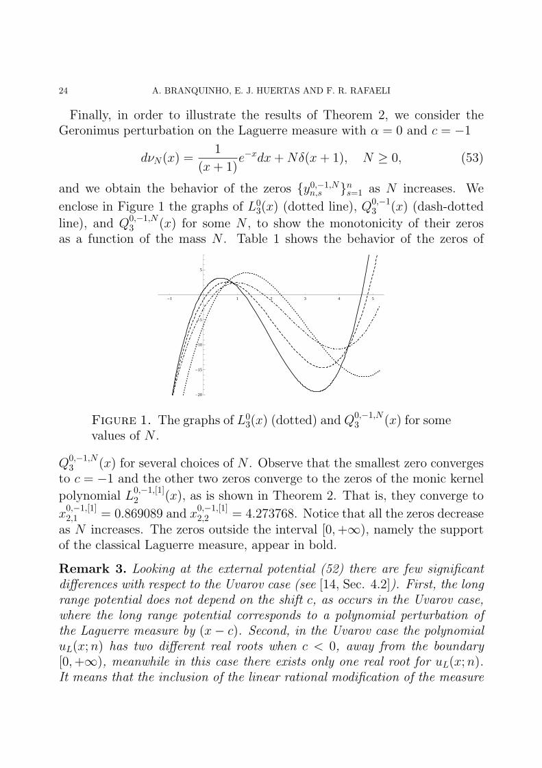
Finally, in order to illustrate the results of Theorem 2, we consider theGeronimus perturbation on the Laguerre measure with α = 0 and c = −1

dνN(x) =1

(x+ 1)e−xdx+Nδ(x+ 1), N ≥ 0, (53)

and we obtain the behavior of the zeros {y0,−1,Nn,s }ns=1 as N increases. We

enclose in Figure 1 the graphs of L03(x) (dotted line), Q0,−1

3 (x) (dash-dotted

line), and Q0,−1,N3 (x) for some N , to show the monotonicity of their zeros

as a function of the mass N . Table 1 shows the behavior of the zeros of

-1 1 2 3 4 5

-20

-15

-10

-5

5

Figure 1. The graphs of L03(x) (dotted) and Q0,−1,N

3 (x) for somevalues of N .

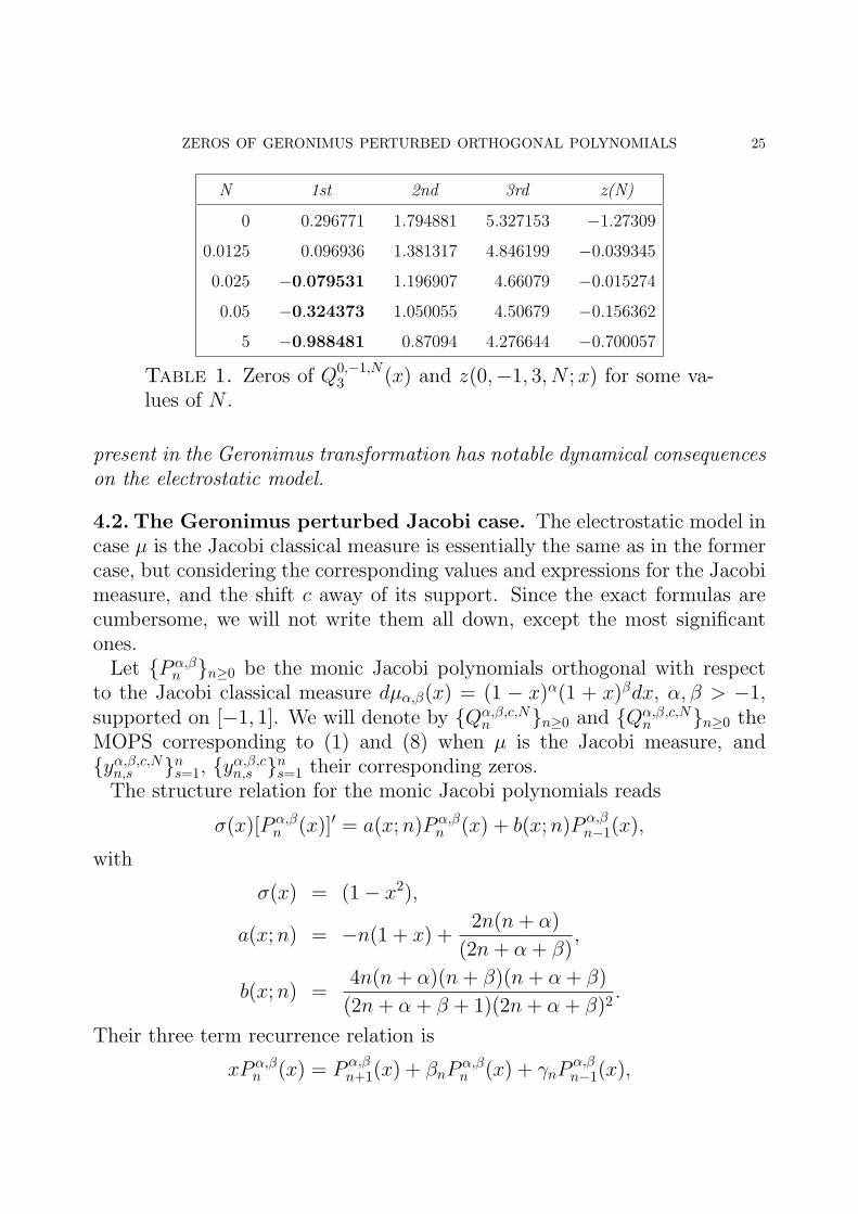
Q0,−1,N3 (x) for several choices of N . Observe that the smallest zero converges

to c = −1 and the other two zeros converge to the zeros of the monic kernel

polynomial L0,−1,[1]2 (x), as is shown in Theorem 2. That is, they converge to

x0,−1,[1]2,1 = 0.869089 and x

0,−1,[1]2,2 = 4.273768. Notice that all the zeros decrease

as N increases. The zeros outside the interval [0,+∞), namely the supportof the classical Laguerre measure, appear in bold.

Remark 3. Looking at the external potential (52) there are few significantdifferences with respect to the Uvarov case (see [14, Sec. 4.2]). First, the longrange potential does not depend on the shift c, as occurs in the Uvarov case,where the long range potential corresponds to a polynomial perturbation ofthe Laguerre measure by (x− c). Second, in the Uvarov case the polynomialuL(x;n) has two different real roots when c < 0, away from the boundary[0,+∞), meanwhile in this case there exists only one real root for uL(x;n).It means that the inclusion of the linear rational modification of the measure


N 1st 2nd 3rd z(N)

0 0.296771 1.794881 5.327153 −1.27309

0.0125 0.096936 1.381317 4.846199 −0.039345

0.025 −0.079531 1.196907 4.66079 −0.015274

0.05 −0.324373 1.050055 4.50679 −0.156362

5 −0.988481 0.87094 4.276644 −0.700057

Table 1. Zeros of Q0,−1,N3 (x) and z(0,−1, 3, N ; x) for some va-

lues of N .

present in the Geronimus transformation has notable dynamical consequenceson the electrostatic model.

4.2. The Geronimus perturbed Jacobi case. The electrostatic model incase µ is the Jacobi classical measure is essentially the same as in the formercase, but considering the corresponding values and expressions for the Jacobimeasure, and the shift c away of its support. Since the exact formulas arecumbersome, we will not write them all down, except the most significantones.Let {P α,β

n }n≥0 be the monic Jacobi polynomials orthogonal with respectto the Jacobi classical measure dµα,β(x) = (1 − x)α(1 + x)βdx, α, β > −1,supported on [−1, 1]. We will denote by {Qα,β,c,N

n }n≥0 and {Qα,β,c,Nn }n≥0 the

MOPS corresponding to (1) and (8) when µ is the Jacobi measure, and{yα,β,c,Nn,s }ns=1, {y

α,β,cn,s }ns=1 their corresponding zeros.

The structure relation for the monic Jacobi polynomials reads

σ(x)[P α,βn (x)]′ = a(x;n)P α,β

n (x) + b(x;n)P α,βn−1(x),

with

σ(x) = (1− x2),

a(x;n) = −n(1 + x) +2n(n+ α)

(2n+ α + β),

b(x;n) =4n(n+ α)(n+ β)(n+ α + β)

(2n+ α + β + 1)(2n+ α + β)2.

Their three term recurrence relation is

xP α,βn (x) = P α,β

n+1(x) + βnPα,βn (x) + γnP

α,βn−1(x),


with

βn = βα,βn =

β2 − α2

(2n+ α + β)(2n+ α + β + 2),

γn = γα,βn =

4n(n+ α)(n+ β)(n+ α + β)

(2n+ α + β − 1)(2n+ α + β)2(2n+ α + β + 1),

and the connection formula (24) for Qα,c,Nn (x) in terms of {Lα

n}n≥0 is

Qα,β,c,Nn (x) = P α,β

n (x) + Λα,β,cn P α,β

n−1(x).

The coefficient of [Qα,β,c,Nn (x)]′ in the holonomic equation is

RL(x;n) = −[uJ ]

′(n; x)

uJ(n; x)−

2x− β (1− x) + α (1 + x)

(1− x)(1 + x),

with

uJ(n; x) = 4n(n+ α)(n+ β)(n+ α + β) (54)

+(2n+ α + β − 1)(2n+ α + β)Λα,β,cn ·

[

(2n+ α + β)2 x+ (α + β) (α− β)

+ (2n+ α + β − 1)(2n+ α + β)Λα,β,cn

]

.

Hence, the electrostatic equilibrium means that the set of zeros {yα,β,c,Nn,s }ns=1

have an equilibrium position under the presence of the external potential

V extJ (x) =

1

2ln uJ(x;n)−

1

2ln (1− x)α+1(1 + x)β+1,

where the first term represents a short range potential corresponding to aunit charge located at the real root

zJ(x;n) = −(α2 − β2)(2n+ α + β) + 4n(n+α)(n+β)(n+α+β)

(2n+α+β−1)Λα,β,cn

(2n+ α + β)3

−(2n+ α + β − 1)(2n+ α + β)2Λα,β,c

n

(2n+ α + β)3

of (54), and the second one is a long range potential associated with theJacobi weight function. Observe that, as in the Laguerre case, the longrange potential does not depend on the shift c.


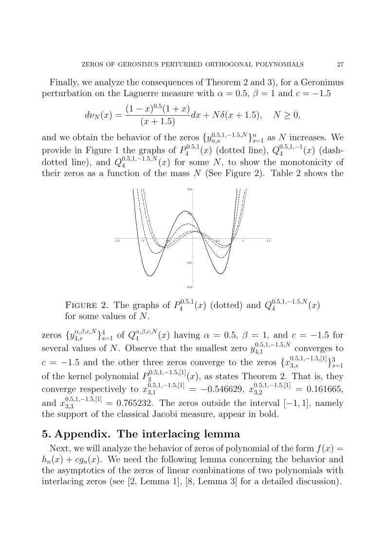
Finally, we analyze the consequences of Theorem 2 and 3), for a Geronimusperturbation on the Laguerre measure with α = 0.5, β = 1 and c = −1.5

dνN(x) =(1− x)0.5(1 + x)

(x+ 1.5)dx+Nδ(x+ 1.5), N ≥ 0,

and we obtain the behavior of the zeros {y0.5,1,−1.5,Nn,s }ns=1 as N increases. We

provide in Figure 1 the graphs of P 0.5,14 (x) (dotted line), Q0.5,1,−1

4 (x) (dash-

dotted line), and Q0.5,1,−1.5,N4 (x) for some N , to show the monotonicity of

their zeros as a function of the mass N (See Figure 2). Table 2 shows the

-1.5 -1 -0.5 0.5 1 1.5

-0.4

-0.2

0.2

0.4

Figure 2. The graphs of P 0.5,14 (x) (dotted) and Q0.5,1,−1.5,N

4 (x)for some values of N .

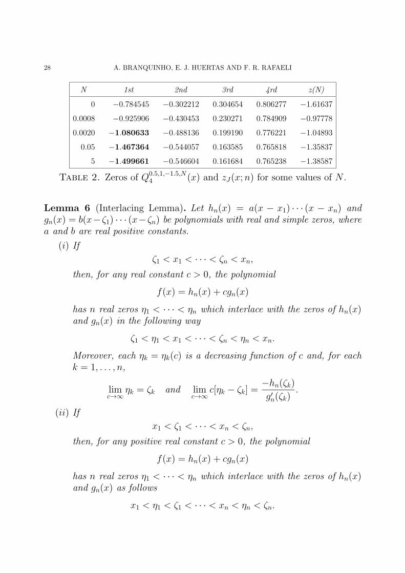
zeros {yα,β,c,N4,s }4s=1 of Qα,β,c,N4 (x) having α = 0.5, β = 1, and c = −1.5 for

several values of N . Observe that the smallest zero y0.5,1,−1.5,N4,1 converges to

c = −1.5 and the other three zeros converge to the zeros {x0.5,1,−1.5,[1]3,s }3s=1

of the kernel polynomial P0.5,1,−1.5,[1]3 (x), as states Theorem 2. That is, they

converge respectively to x0.5,1,−1.5,[1]3,1 = −0.546629, x

0.5,1,−1.5,[1]3,2 = 0.161665,

and x0.5,1,−1.5,[1]3,3 = 0.765232. The zeros outside the interval [−1, 1], namely

the support of the classical Jacobi measure, appear in bold.

5. Appendix. The interlacing lemma

Next, we will analyze the behavior of zeros of polynomial of the form f(x) =hn(x) + cgn(x). We need the following lemma concerning the behavior andthe asymptotics of the zeros of linear combinations of two polynomials withinterlacing zeros (see [2, Lemma 1], [8, Lemma 3] for a detailed discussion).


N 1st 2nd 3rd 4rd z(N)

0 −0.784545 −0.302212 0.304654 0.806277 −1.61637

0.0008 −0.925906 −0.430453 0.230271 0.784909 −0.97778

0.0020 −1.080633 −0.488136 0.199190 0.776221 −1.04893

0.05 −1.467364 −0.544057 0.163585 0.765818 −1.35837

5 −1.499661 −0.546604 0.161684 0.765238 −1.38587

Table 2. Zeros of Q0.5,1,−1.5,N4 (x) and zJ(x;n) for some values of N .

Lemma 6 (Interlacing Lemma). Let hn(x) = a(x − x1) · · · (x − xn) andgn(x) = b(x−ζ1) · · · (x−ζn) be polynomials with real and simple zeros, wherea and b are real positive constants.

(i) If

ζ1 < x1 < · · · < ζn < xn,

then, for any real constant c > 0, the polynomial

f(x) = hn(x) + cgn(x)

has n real zeros η1 < · · · < ηn which interlace with the zeros of hn(x)and gn(x) in the following way

ζ1 < η1 < x1 < · · · < ζn < ηn < xn.

Moreover, each ηk = ηk(c) is a decreasing function of c and, for eachk = 1, . . . , n,

limc→∞

ηk = ζk and limc→∞

c[ηk − ζk] =−hn(ζk)

g′n(ζk).

(ii) If

x1 < ζ1 < · · · < xn < ζn,

then, for any positive real constant c > 0, the polynomial

f(x) = hn(x) + cgn(x)

has n real zeros η1 < · · · < ηn which interlace with the zeros of hn(x)and gn(x) as follows

x1 < η1 < ζ1 < · · · < xn < ηn < ζn.


Moreover, each ηk = ηk(c) is an increasing function of c and, for eachk = 1, . . . , n,

limc→∞

ηk = ζk and limc→∞

c[ζk − ηk] =hn(ζk)

g′n(ζk).

References[1] D. Barrios and A. Branquinho, Complex high order Toda and Volterra lattices, J. Difference

Equ. Appl. 15 (2) (2009), 197–213.[2] C. F. Bracciali, D. K. Dimitrov, and A. Sri Ranga, Chain sequences and symmetric generalized

orthogonal polynomials, J. Comput. Appl. Math. 143 (2002), 95–106.[3] A. Branquinho and F. Marcellan, Generating new classes of orthogonal polynomials, Int. J.

Math. Math. Sci. 19 (4) (1996), 643–656.[4] M. I. Bueno, A. Deano, and E. Tavernetti, A new algorithm for computing the Geronimus

transformation with large shifts, Numer. Alg. 54 (2010), 101–139.[5] M. I. Bueno and F. Marcellan, Darboux tranformations and perturbation of linear functionals,

Linear Algebra Appl. 384 (2004), 215–242.[6] T. S. Chihara, An Introduction to Orthogonal Polynomials. Mathematics and its Applications

Series, Gordon and Breach, New York, 1978.[7] M. Derevyagin and F. Marcellan, A note on the Geronimus transformation and Sobolev or-

thogonal polynomials, Numer. Algorithms, DOI 10.1007/s11075-013-9788-6, (2013), 1-17.[8] D. K. Dimitrov, M. V. Mello, and F. R. Rafaeli, Monotonicity of zeros of Jacobi-Sobolev type

orthogonal polynomials, Appl. Numer. Math. 60 (2010), 263–276.[9] J. Dini, P. Maroni, La multiplication d’une forme lineaire par une forme rationnelle. Applica-

tion aux polynomes de Laguerre-Hahn, Ann. Polon. Math. 52 (1990), 175–185.[10] W. Gautschi, Orthogonal Polynomials: Computation and Approximation, in Numerical Math-

ematics and Scientific Computation Series, Oxford University Press. New York. 2004.[11] Y. L. Geronimus, On the polynomials orthogonal with respect to a given number sequence and

a theorem, in: W. Hahn and I. A. Nauk, (eds.), vol. 4 (1940), 215–228 (in Russian).[12] Y. L. Geronimus, On the polynomials orthogonal with respect to a given number sequence, Zap.

Mat. Otdel. Khar’kov. Univers. i NII Mat. i Mehan. 17 (1940), 3–18.[13] F. A. Grunbaum, Variations on a theme of Heine and Stieltjes: An electrotatic interpretation

of the zeros of certain polynomials, J. Comp. Appl. Math. 99 (1998), 189–194.[14] E. J. Huertas, F. Marcellan and F. R. Rafaeli, Zeros of orthogonal polynomials generated by

canonical perturbations of measures, Appl. Math. Comput. 218 (13) (2012), 7109-7127.[15] E. Hendriksen and H. Van Rossum, Semiclassical orthogonal polynomials, Lect. Notes in Math.,

Springer Verlag (1985) Vol. 1171, Cl. Brezinski et coll. ed., p. 354–361.[16] M. E. H. Ismail, More on electrostatic models for zeros of orthogonal polynomials, Numer.

Funct. Anal. Optimiz. 21 (2000), 191–204.[17] M. E. H. Ismail, Classical and Quantum Orthogonal Polynomials in One Variable, Encyclo-

pedia of Mathematics and its Applications, Vol. 98. Cambridge University Press, CambridgeUK. 2005.

[18] F. Marcellan and P. Maroni, Sur l’adjonction d’ une masse de Dirac a une forme reguliere et

semi-classique, Annal. Mat. Pura ed Appl. 162 (1992), 1–22.[19] P. Maroni, Sur la suite de polynomes orthogonaux associee a la forme u = δc + λ(x− c)−1L,

Period. Math. Hungar. 21 (3) (1990), 223–248.


[20] P. Maroni, Une theorie algebrique des polynomes orthogonaux. Application aux polynomes

orthogonaux semi-classiques, inOrthogonal Polynomials and Their Applications, C. Brezinskiet al. Editors. Annals. Comput. Appl. Math. 9. Baltzer, Basel. 1991, 95–130.

[21] A. Ronveaux and F. Marcellan, Differential equation for classical-type orthogonal polynomials,Canad. Math. Bull. 32 (4), (1989), 404–411.

[22] J. Shohat, On mechanical quadratures, in particular, with positive coefficients, Trans. Amer.Math. Soc. 42 (3) (1937), 461–496.

[23] V. Spiridonov, A. Zhedanov, Discrete Darboux transformations, the discrete-time Toda lattice,

and the Askey-Wilson polynomials, Methods Appl. Anal. 2 (4) (1995), 369–398.[24] V. Spiridonov, A. Zhedanov, Discrete-time Volterra chain and classical orthogonal polyno-

mials, J. Phys. A: Math. Gen. 30 (1997), 8727–8737.[25] G. Szego, Orthogonal Polynomials, Amer. Math. Soc. Coll. Publ, Vol. 23, 4th ed., Amer.

Math. Soc., Providence, RI, 1975.[26] V. B. Uvarov, The connection between systems of polynomials orthogonal with respect to dif-

ferent distribution functions, USSR Compt. Math. Phys. 9 (6) (1969), 25–36.[27] A. Zhedanov, Rational spectral transformations and orthogonal polynomials, J. Comput. Appl.

Math. 85 (1997), 67–83.[28] G. J. Yoon,Darboux transforms and orthogonal polynomials, Bull. Korean Math. Soc. 39

(2002), 359–376.

Amılcar Branquinho

CMUC, Department of Mathematics, Universidade de Coimbra, FCTUC, Largo D. Dinis,

3001-454 Coimbra, Portugal

E-mail address : [email protected]

Edmundo J. Huertas

CMUC, Department of Mathematics, Universidade de Coimbra, FCTUC, Largo D. Dinis,

3001-454 Coimbra, Portugal


Fernando R. Rafaeli

Departamento de Matematica Aplicada, IBILCE, Universidade Estadual Paulista, Brazil


Documents

ZEROS OF ORTHOGONAL POLYNOMIALS GENERATED · ZEROS OF ORTHOGONAL POLYNOMIALS GENERATED ... (x−c) dµ(x)+Nδ ... sharp bounds and speed of convergence to them for their