Embed Size (px)
Citation preview
ZFC Preparation DocumentationRelease 0
Samuel Bowers
Feb 25, 2019

Contents
1 Objectives 3
2 Contents 5
3 Requirements 33
4 Contact 35
i

ii
ZFC Preparation Documentation, Release 0
Welcome to the preparation materials for the workshop for the study of drivers of deforestation, forest degradation andnational forest definition. The workshop will take place in Harare on 25th February - 1st March 2019. To prepare forthe workshop, we’ve prepared some material for you to work through.
For part of the workshop we’ll be covering the basics of R, a programming language commonly used for data analysis.We’ll be running it through the ‘RStudio’ development environment, and using it for the analysis of forest inventorydata from Zimbabwe. The purpose of this document is to prepare all participants by installing required software andfamiliarisation with RStudio’s user interface. We’ll also run through the installation process of QGIS.
We’d like all participants to have at least tried to run through these instructions before the workshop begins on Monday25th February.
Contents 1
ZFC Preparation Documentation, Release 0
2 Contents
CHAPTER 1
Objectives
1. To install RStudio and QGIS in preparation for the workshop
2. To familiarise each participant with the layout and operation of RStudio
3. To produce some simple summary statistics and graphs using forest inventory data
3

ZFC Preparation Documentation, Release 0
4 Chapter 1. Objectives
CHAPTER 2
Contents
2.1 RStudio Setup
2.1.1 Downloading R
The first step is to download the R software. You can download it for free from CRAN via the R website.
If you’re confused about which version you need, you can download the Windows (32-bit/64-bit) version here (79MB).
2.1.2 Installing R
Once the download is complete, navigate to your Downloads folder, and run the executable named R-3.5.2-win.exe (or similar).
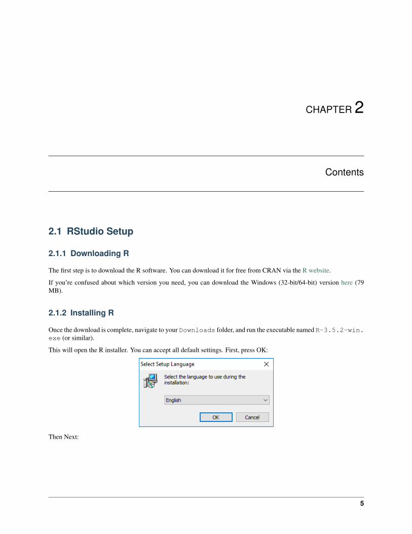
This will open the R installer. You can accept all default settings. First, press OK:
Then Next:
5
ZFC Preparation Documentation, Release 0
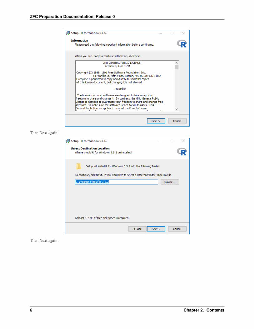
Then Next again:
Then Next again:
6 Chapter 2. Contents
ZFC Preparation Documentation, Release 0
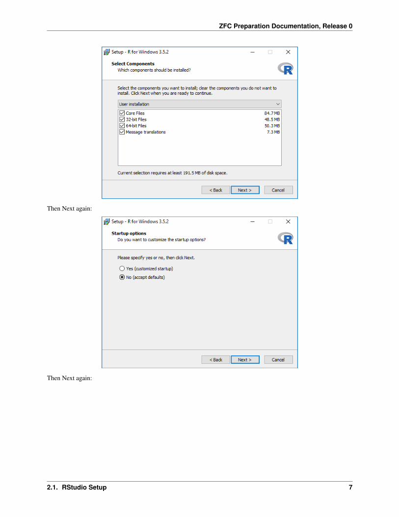
Then Next again:
Then Next again:
2.1. RStudio Setup 7
ZFC Preparation Documentation, Release 0
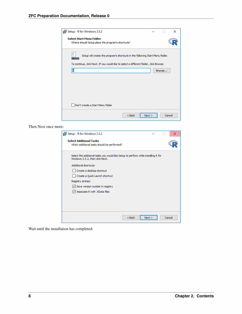
Then Next once more:
Wait until the installation has completed:
8 Chapter 2. Contents
ZFC Preparation Documentation, Release 0
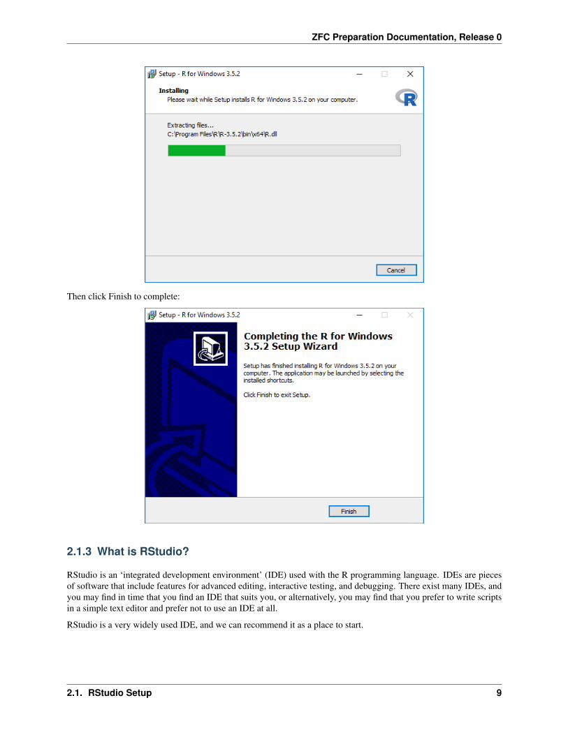
Then click Finish to complete:
2.1.3 What is RStudio?
RStudio is an ‘integrated development environment’ (IDE) used with the R programming language. IDEs are piecesof software that include features for advanced editing, interactive testing, and debugging. There exist many IDEs, andyou may find in time that you find an IDE that suits you, or alternatively, you may find that you prefer to write scriptsin a simple text editor and prefer not to use an IDE at all.
RStudio is a very widely used IDE, and we can recommend it as a place to start.
2.1. RStudio Setup 9
ZFC Preparation Documentation, Release 0
2.1.4 Downloading RStudio
You can download RStudio for free from the RStudio website. Make sure you choose the correct version, which isRStudio Desktop installer (free) for Windows Vista/7/8/10.
If you’re struggling to find the correct version, you can also download it directly here (85.8 MB).
Note: Are you using Linux or Mac, or an earlier version of Windows? The following instructions should mostly workfine for you, but be aware you’ll need to select a different version from the RStudio download site, and that RStudiowill look visually slightly different.
2.1.5 Installing RStudio
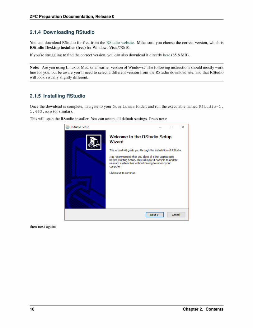
Once the download is complete, navigate to your Downloads folder, and run the executable named RStudio-1.1.463.exe (or similar).
This will open the RStudio installer. You can accept all default settings. Press next:
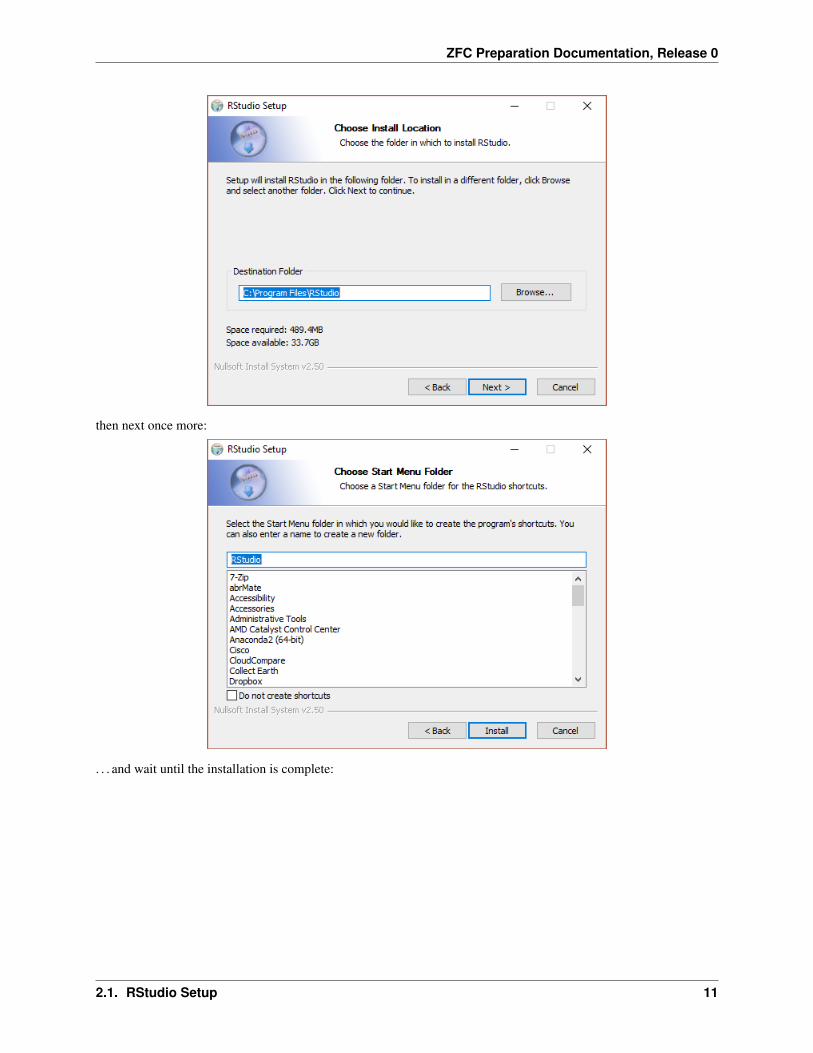
then next again:
10 Chapter 2. Contents
ZFC Preparation Documentation, Release 0
then next once more:
. . . and wait until the installation is complete:
2.1. RStudio Setup 11
ZFC Preparation Documentation, Release 0
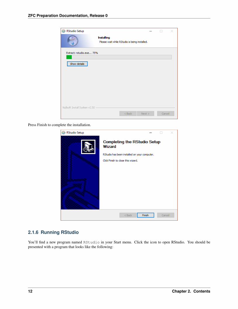
Press Finish to complete the installation.
2.1.6 Running RStudio
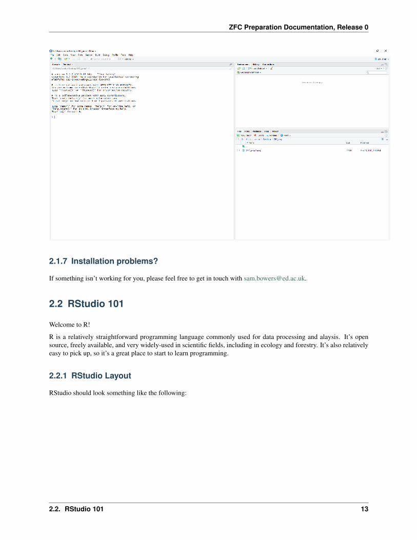
You’ll find a new program named RStudio in your Start menu. Click the icon to open RStudio. You should bepresented with a program that looks like the following:
12 Chapter 2. Contents
ZFC Preparation Documentation, Release 0
2.1.7 Installation problems?
If something isn’t working for you, please feel free to get in touch with [email protected].
2.2 RStudio 101
Welcome to R!
R is a relatively straightforward programming language commonly used for data processing and alaysis. It’s opensource, freely available, and very widely-used in scientific fields, including in ecology and forestry. It’s also relativelyeasy to pick up, so it’s a great place to start to learn programming.
2.2.1 RStudio Layout
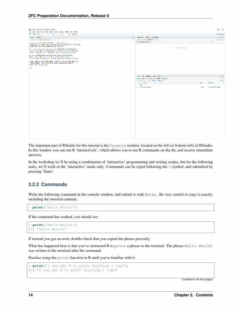
RStudio should look something like the following:
2.2. RStudio 101 13
ZFC Preparation Documentation, Release 0
The important part of RStudio for this tutorial is the Console window, located on the left (or bottom-left) of RStudio.In this window you can run R ‘interactively’, which allows you to run R commands on-the-fly, and receive immediateanswers.
In the workshop we’ll be using a combination of ‘interactive’ programming and writing scripts, but for the followingtasks, we’ll work in the ‘interactive’ mode only. Commands can be typed following the > symbol, and submitted bypressing ‘Enter’.
2.2.2 Commands
Write the following command in the console window, and submit it with Enter. Be very careful to copy it exactly,including the inverted commas.
> print('Hello World!')
If the command has worked, you should see:
> print('Hello World!')[1] "Hello World!"
If instead you got an error, double-check that you copied the phrase precisely.
What has happened here is that you’ve instructed R to print a phrase to the terminal. The phrase Hello World!was written to the terminal after the command.
Practice using the print function in R until you’re familiar with it:
> print('I can get R to print anything I type')[1] "I can get R to print anything I type"
(continues on next page)
14 Chapter 2. Contents
ZFC Preparation Documentation, Release 0
(continued from previous page)
> print('Even numbers like 6 and symbols like #')[1] "Even numbers like 6 and symbols like #"
There are hundreds of other commands available in R (commonly known as ‘functions’). What do you think thefollowing functiuons do?:
> toupper('Hello World!')[1] "HELLO WORLD!"
> nchar('Hello World!')[1] 12
> paste('Hello', 'World!')[1] "Hello World!"
Tip: You can access help for R functions using a ? symbol in the console window. For example: ?print, ?toupper etc. This will bring up a text description of how the function works, and what inputs it requires.
An aside: Comments
Comments are important aspects of programs. Comments are used to describe what your program does in readablelanguage, or to temporarily remove lines from a program. Comments are indicated by the # symbol, and anything thatfollows won’t be executed.
We’ll now use comments to describe the code. Adding comments to your code is good practice as it makes your codeeasier for other people to use, and helps you to remember how your own code works. For the purposes of this tutorial,you won’t need to copy out anything after the # symbol.
2.2.3 Calculations
Until now you’ve been working with letters and symbols, a data type in R known as characters. R is also able tohandle numbers, which are represented by the data types named integer (for whole numbers) and numeric (fornumbers with a decimal point.
Attention: Unlike characters, integer and numeric data types are not surrounded by inverted commas.
We can use R like a calculator to perform arthimetic on numbers. Try the following:
> 1 + 2 # Addition[1] 3
> 1 - 2 # Subtraction[1] -1
> 3 * 4 # Multiplication[1] 12
> 5 / 2 # Division[1] 2.5
2.2. RStudio 101 15
ZFC Preparation Documentation, Release 0
We can also use R to peform more complex operations:
> 8 ^ 2 # Power functions[1] 64
> log(10) # Natural logarithm[1] 2.302585
> pi # Access constants[1] 3.141593
2.2.4 Variables
In programming, variables are names that we give for something. They ensure that code is readable, and offer a meansof ‘saving’ a value for later use. We assign a value to a variable in R either using the = or <- symbols, with the variablename on the left and it’s value on the right. Try these examples of how variables work:
> x <- 1
> x[1] 1
> y <- 1 + 2
> y[1] 3
> z <- x + y
> z[1] 4
Exercises
1. Use the +, -, *, and - operators to compute the following:
• 123456 plus 654321
• 123456 minus 654321
• 123456 multiplied by 654321
• 123456 divided by 654321
• 123456 squared
2. The basal area of a tree (BA) can be calculated using the equation:
• BA = 𝜋(DBH/2)^2
. . . where DBH is the tree diameter at breast height and 𝜋 = 3.14. Use R to calculate the basal area of atree of 50 cm DBH.
2.2.5 Logical data
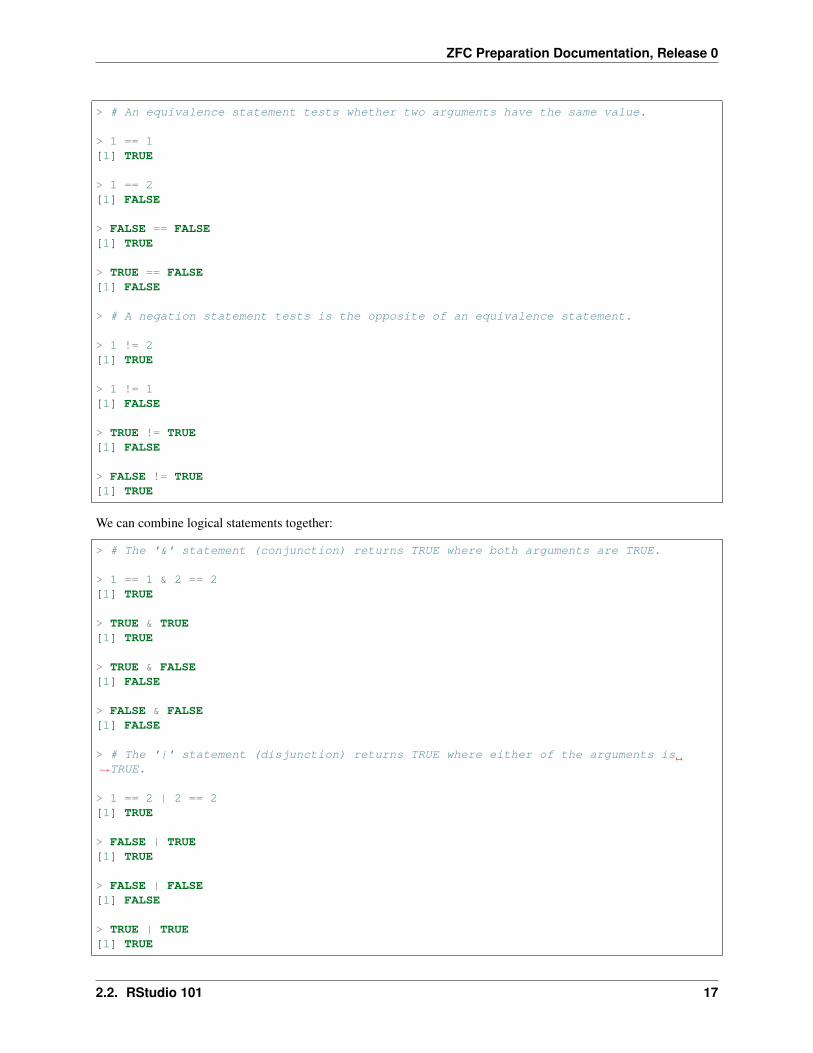
Logical data can take two values; TRUE or FALSE (sometimes denoted as 1 or 0). The logical data type is mostcommonly associated with logical expressions. The main logical expressions we use in R are as follows:
16 Chapter 2. Contents
ZFC Preparation Documentation, Release 0
> # An equivalence statement tests whether two arguments have the same value.
> 1 == 1[1] TRUE
> 1 == 2[1] FALSE
> FALSE == FALSE[1] TRUE
> TRUE == FALSE[1] FALSE
> # A negation statement tests is the opposite of an equivalence statement.
> 1 != 2[1] TRUE
> 1 != 1[1] FALSE
> TRUE != TRUE[1] FALSE
> FALSE != TRUE[1] TRUE
We can combine logical statements together:
> # The '&' statement (conjunction) returns TRUE where both arguments are TRUE.
> 1 == 1 & 2 == 2[1] TRUE
> TRUE & TRUE[1] TRUE
> TRUE & FALSE[1] FALSE
> FALSE & FALSE[1] FALSE
> # The '|' statement (disjunction) returns TRUE where either of the arguments is→˓TRUE.
> 1 == 2 | 2 == 2[1] TRUE
> FALSE | TRUE[1] TRUE
> FALSE | FALSE[1] FALSE
> TRUE | TRUE[1] TRUE
2.2. RStudio 101 17
ZFC Preparation Documentation, Release 0
Logical statements like these may be quite different from anything you’ve learned before, so don’t worry if this is stillconfusing!
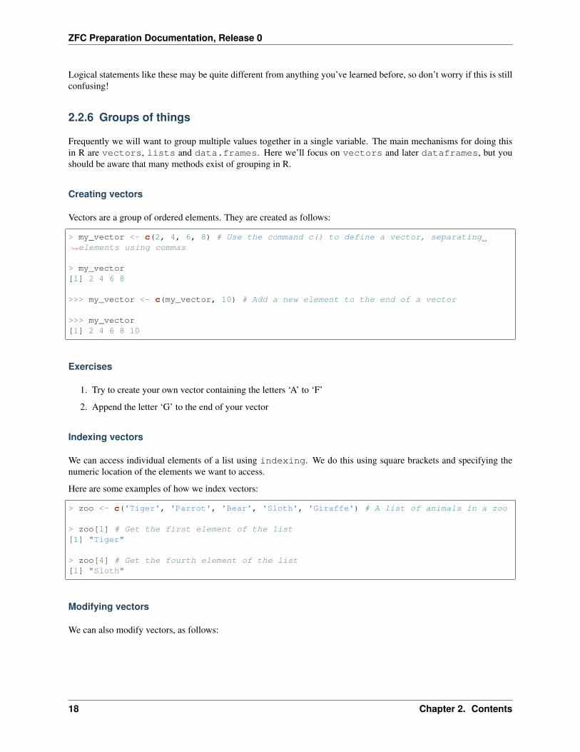
2.2.6 Groups of things
Frequently we will want to group multiple values together in a single variable. The main mechanisms for doing thisin R are vectors, lists and data.frames. Here we’ll focus on vectors and later dataframes, but youshould be aware that many methods exist of grouping in R.
Creating vectors
Vectors are a group of ordered elements. They are created as follows:
> my_vector <- c(2, 4, 6, 8) # Use the command c() to define a vector, separating→˓elements using commas
> my_vector[1] 2 4 6 8
>>> my_vector <- c(my_vector, 10) # Add a new element to the end of a vector
>>> my_vector[1] 2 4 6 8 10
Exercises
1. Try to create your own vector containing the letters ‘A’ to ‘F’
2. Append the letter ‘G’ to the end of your vector
Indexing vectors
We can access individual elements of a list using indexing. We do this using square brackets and specifying thenumeric location of the elements we want to access.
Here are some examples of how we index vectors:
> zoo <- c('Tiger', 'Parrot', 'Bear', 'Sloth', 'Giraffe') # A list of animals in a zoo
> zoo[1] # Get the first element of the list[1] "Tiger"
> zoo[4] # Get the fourth element of the list[1] "Sloth"
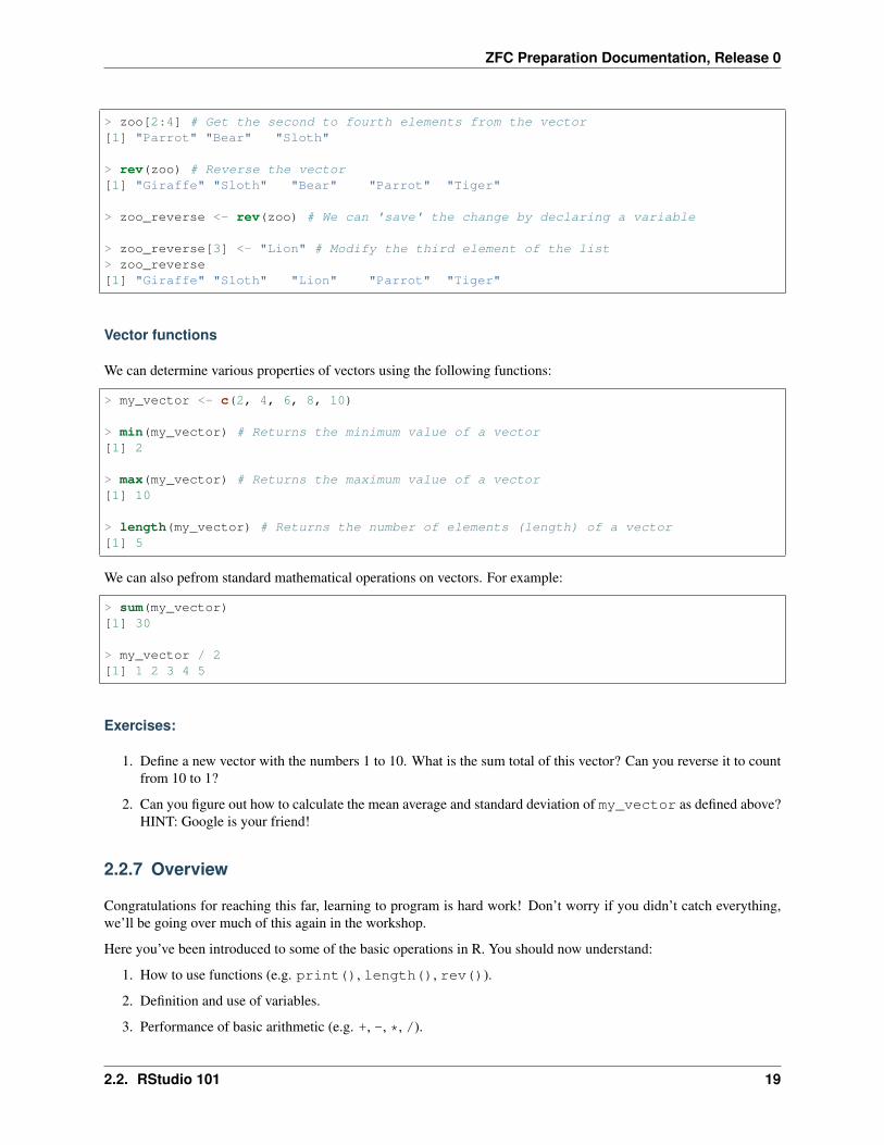
Modifying vectors
We can also modify vectors, as follows:
18 Chapter 2. Contents
ZFC Preparation Documentation, Release 0
> zoo[2:4] # Get the second to fourth elements from the vector[1] "Parrot" "Bear" "Sloth"
> rev(zoo) # Reverse the vector[1] "Giraffe" "Sloth" "Bear" "Parrot" "Tiger"
> zoo_reverse <- rev(zoo) # We can 'save' the change by declaring a variable
> zoo_reverse[3] <- "Lion" # Modify the third element of the list> zoo_reverse[1] "Giraffe" "Sloth" "Lion" "Parrot" "Tiger"
Vector functions
We can determine various properties of vectors using the following functions:
> my_vector <- c(2, 4, 6, 8, 10)
> min(my_vector) # Returns the minimum value of a vector[1] 2
> max(my_vector) # Returns the maximum value of a vector[1] 10
> length(my_vector) # Returns the number of elements (length) of a vector[1] 5
We can also pefrom standard mathematical operations on vectors. For example:
> sum(my_vector)[1] 30
> my_vector / 2[1] 1 2 3 4 5
Exercises:
1. Define a new vector with the numbers 1 to 10. What is the sum total of this vector? Can you reverse it to countfrom 10 to 1?
2. Can you figure out how to calculate the mean average and standard deviation of my_vector as defined above?HINT: Google is your friend!
2.2.7 Overview
Congratulations for reaching this far, learning to program is hard work! Don’t worry if you didn’t catch everything,we’ll be going over much of this again in the workshop.
Here you’ve been introduced to some of the basic operations in R. You should now understand:
1. How to use functions (e.g. print(), length(), rev()).
2. Definition and use of variables.
3. Performance of basic arithmetic (e.g. +, -, *, /).
2.2. RStudio 101 19
ZFC Preparation Documentation, Release 0
4. How boolean logic works in R (i.e. TRUE, FALSE).
5. How to use vectors to store multiple values together (e.g. c(1,2,3)), access individual elements of vectors,and perform mathematical operations on all values of a vector.
In the remainder of this introduction to R we’ll load some synthetic forest inventory data in R, perform basic statisticalanalyses, and learn to draw plots.
2.3 RStudio Data Processing
In this second part, we’ll perform some basic processing on some synthetic forest inventory data.
2.3.1 Load external data into R
The most straightforward way to load data into R is to use comma-separated values (.csv) format, a text file formatthat separates records across rows and fields with commas. CSV files can be exported from spreadsheet software (e.g.Microsoft Excel).
The .csv file we’ll use is named plot_data.csv, and can be downloaded here.
Save plot_data.csv somewhere memorable (e.g. Desktop). You can open this file with a text editor (e.g.Notepad) or as a spreadsheet (e.g. Microsoft Excel) if you’d like to take a look at its contents.
This file contains synthetic data for 25 forest plots in miombo woodlands each sized 50 x 50 m (0.25 ha). Each rowcontains data for a unique stem, where stems have a range of properties (e.g. DBH, height, species, etc.).
Attention: The data we’ll use in this exercise is entirely made up. Definitely don’t use this dataset for anyquantitative work!
To load the data into R, we’ll need two commands. First, we’ll need to set the ‘working directory’, which is thelocation that R will run and where we will reference the CSV file relative to.
Set the working directory to the location you saved the data to as follows:
> setwd('C:/Users/your_username/Desktop/')
Note:
• Make your you replace your_username with your actual username.
• Note that the directory is referenced with / rather than \, this is because \ has a special meaning in R.
• If you saved plot_data.csv at any location other than the Desktop, you’ll need to reference that locationinstead.
To load the data into R, you can use the read.csv() function, as follows. Be careful with inverted commas, anddon’t worry for now about what stringsAsFactors = FALSE means:
> df <- read.csv('plot_data.csv', stringsAsFactors = FALSE)
Once you’ve successfully loaded in the data, you can take a peek at the first few lines of it using the head() command:
20 Chapter 2. Contents
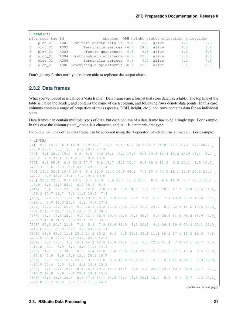
ZFC Preparation Documentation, Release 0
> head(df)plot_code tag_id species DBH height status x_location y_location1 plot_01 A001 Parinari curatellifolia 9.8 12.0 alive 1.2 1.92 plot_01 A002 Terminalia sericea 44.9 24.0 alive 4.3 3.43 plot_01 A003 Afzelia quanzensis 6.3 8.5 alive 1.6 3.84 plot_01 A004 Erythrophleum africanum 16.9 20.0 alive 2.0 4.65 plot_01 A005 Terminalia sericea 9.9 9.0 alive 0.1 7.56 plot_01 A006 Brachystegia spiciformis 30.7 22.0 alive 3.1 8.3
Don’t go any further until you’ve been able to replicate the output above.
2.3.2 Data frames
What you’ve loaded in is callled a ‘data frame’. Data frames are a format that store data like a table. The top line of thetable is called the header, and contains the name of each column, and following rows denote data points. In this case,columns contain a range of properties of trees (species, DBH, height, etc.), and rows contains data for an individualstem.
Data frames can contain multiple types of data, but each column of a data frame has to be a single type. For example,in this case the column plot_code is a character, and DBH is a numeric data type.
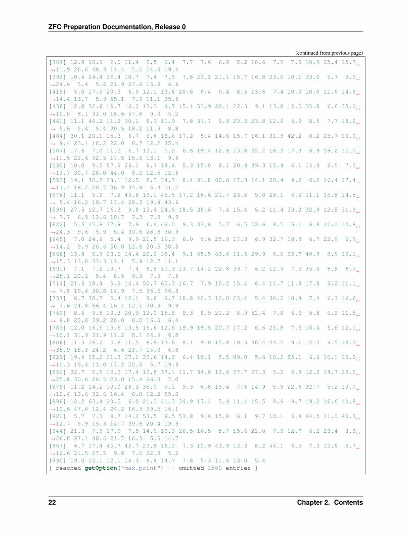
Individual columns of the data frame can be accessed using the $ operator, which returns a vector. For example:
> df$DBH[1] 9.8 44.9 6.3 16.9 9.9 30.7 6.9 9.1 6.9 20.6 28.7 45.8 5.7 12.8 9.7 20.7→˓8.9 13.5 5.5 5.5 6.2 10.3 27.9[24] 6.1 36.7 19.2 5.5 8.5 5.6 38.6 17.2 17.3 9.1 24.3 12.4 13.0 15.9 16.4 8.2→˓6.2 7.0 31.4 6.1 41.5 8.0 28.0[47] 6.3 85.6 8.2 53.5 37.7 9.8 16.7 13.3 10.0 6.6 19.2 11.9 9.2 14.1 8.0 10.0→˓23.3 9.6 5.3 18.4 27.0 23.8 71.4[70] 13.0 52.1 13.8 23.6 6.4 11.9 13.4 10.6 44.2 7.5 10.6 44.5 11.1 13.9 24.5 25.0→˓7.2 8.9 42.1 13.1 17.7 19.7 19.0[93] 21.8 22.0 9.7 23.6 8.1 15.0 5.6 23.7 15.9 21.5 8.2 8.6 14.9 7.7 13.5 12.1→˓5.8 6.8 15.5 83.2 6.9 35.6 8.4[116] 6.4 9.7 22.8 16.8 12.8 5.8 29.0 5.8 14.0 5.2 12.8 10.6 17.7 8.0 23.4 31.4→˓26.2 17.7 18.7 7.1 11.5 29.5 7.4[139] 9.3 13.0 11.4 18.1 49.7 6.7 5.9 23.4 7.9 5.4 6.3 7.1 13.8 27.6 13.6 9.7→˓16.1 5.0 48.0 26.0 6.1 6.7 17.3[162] 19.0 12.3 21.6 5.0 16.5 28.2 22.3 18.5 17.4 31.6 23.7 8.0 22.5 14.6 19.5 13.8→˓74.2 13.7 24.7 18.0 10.8 11.4 30.3[185] 11.2 17.8 38.4 9.4 32.1 16.9 19.4 11.6 17.1 35.3 6.5 28.6 11.5 38.6 15.9 7.5→˓ 9.2 40.8 11.5 8.9 22.1 12.3 35.2[208] 27.3 20.7 21.3 7.1 5.4 7.9 16.6 31.0 6.0 30.3 9.4 26.8 19.9 22.4 22.1 49.0→˓13.6 28.1 28.8 6.5 9.9 23.2 21.4[231] 19.6 49.0 11.1 25.4 14.2 10.2 9.4 5.8 38.1 33.1 11.1 16.1 17.1 15.5 19.5 7.8→˓20.5 28.0 29.3 9.1 44.0 24.3 42.3[254] 9.2 15.7 7.2 16.1 44.2 18.2 15.9 34.4 5.5 7.5 12.2 11.4 7.8 20.1 39.7 6.3→˓10.8 9.1 6.9 8.2 5.3 11.1 14.4[277] 31.7 5.6 20.5 16.3 5.4 12.0 7.4 19.5 16.4 27.9 15.6 22.9 57.1 15.4 6.5 13.0→˓33.0 7.9 8.9 19.6 12.4 20.1 16.7[300] 6.7 5.9 12.4 23.5 9.5 13.8 5.4 40.9 22.0 31.0 19.8 6.7 41.4 42.1 5.9 30.9→˓20.9 40.4 6.5 8.1 8.2 14.9 15.2[323] 7.4 19.1 18.6 10.1 18.1 19.2 44.7 41.4 7.4 5.3 22.2 19.7 10.6 39.2 20.7 8.1→˓15.2 12.8 7.9 6.1 27.1 19.4 15.2[346] 16.0 44.5 20.3 8.1 47.8 11.1 11.6 11.4 18.6 25.1 10.4 5.5 9.1 8.7 7.3 12.2→˓26.8 25.2 17.8 9.2 11.6 11.9 24.0
(continues on next page)
2.3. RStudio Data Processing 21
ZFC Preparation Documentation, Release 0
(continued from previous page)
[369] 12.8 18.9 9.0 11.4 9.5 9.4 7.7 7.6 6.9 5.2 10.6 7.9 7.0 18.9 25.4 15.7→˓11.9 26.6 48.3 11.4 5.2 24.0 19.4[392] 10.4 24.4 36.4 10.7 7.4 7.5 7.8 23.1 21.1 15.7 16.8 23.0 10.1 33.0 5.7 9.5→˓24.6 5.4 5.6 21.9 27.6 15.9 6.6[415] 5.0 17.5 20.3 6.5 12.1 13.6 20.6 9.4 9.4 8.5 13.6 7.4 10.0 10.0 11.6 14.8→˓14.4 13.7 5.9 55.1 7.9 11.1 35.6[438] 12.8 32.6 19.7 16.2 13.3 9.7 15.1 53.9 28.1 22.3 9.1 13.8 12.5 35.0 6.6 33.0→˓10.0 8.1 31.0 18.6 57.8 9.0 5.2[461] 11.1 46.2 11.2 30.1 8.3 11.9 7.8 37.7 9.9 23.3 23.8 12.9 5.9 8.5 7.7 18.2→˓ 5.6 5.4 5.4 30.5 18.2 11.9 8.8[484] 30.1 20.1 15.3 6.7 6.6 18.6 17.2 5.4 14.6 15.7 16.1 31.9 42.2 8.2 25.7 20.0→˓ 9.4 23.1 18.2 22.0 8.7 12.2 35.4[507] 17.6 7.0 11.5 6.7 13.1 5.2 6.6 19.4 12.8 13.8 32.2 16.3 17.3 6.9 59.2 15.5→˓11.5 22.4 32.5 17.5 15.6 13.1 9.6[530] 10.0 9.5 57.9 26.1 6.7 18.6 5.3 15.0 8.1 20.9 39.3 15.4 6.1 15.9 6.5 7.5→˓13.7 30.7 28.0 44.0 8.2 12.5 12.5[553] 19.1 30.7 28.1 12.5 8.3 34.7 8.4 81.8 60.6 17.3 14.1 20.4 9.2 6.2 16.4 27.4→˓13.4 18.2 20.7 36.9 34.9 6.4 51.2[576] 11.1 5.2 7.2 43.8 19.1 45.5 17.2 16.6 21.7 23.8 5.0 28.1 6.0 11.1 16.8 14.5→˓ 5.4 16.2 10.7 17.4 28.3 19.4 43.6[599] 27.5 12.7 16.3 9.8 13.4 24.6 18.5 38.6 7.4 15.4 5.2 11.4 33.2 32.9 12.8 31.9→˓ 7.7 6.9 13.6 10.7 7.3 7.0 9.9[622] 5.5 15.8 37.9 7.9 6.4 49.0 9.3 33.6 5.7 6.5 52.6 8.5 5.1 6.8 12.0 10.8→˓24.3 9.6 5.9 5.4 30.6 28.8 30.9[645] 7.0 24.8 5.4 9.9 21.5 16.3 6.0 9.6 25.9 17.3 6.9 32.7 18.3 6.7 22.9 6.9→˓14.2 9.9 26.6 50.8 12.8 20.5 38.5[668] 13.8 5.9 23.0 14.4 20.0 35.4 9.1 65.5 43.6 11.6 29.9 6.0 25.7 40.9 8.9 19.1→˓15.3 13.8 33.3 11.1 5.9 12.7 11.1[691] 7.1 7.2 10.7 7.4 6.8 10.3 13.7 14.2 22.8 33.7 6.2 12.9 7.3 35.0 8.9 6.5→˓25.1 20.2 5.4 8.5 9.3 7.9 7.5[714] 21.6 18.4 5.9 14.4 50.7 60.3 16.7 7.9 10.2 15.4 6.4 11.7 11.8 17.8 9.2 11.1→˓ 7.8 19.4 30.8 14.9 7.5 36.6 66.8[737] 8.7 38.7 5.4 12.1 9.8 9.7 10.8 40.3 10.0 23.4 5.4 36.2 10.4 7.4 6.3 16.6→˓ 7.6 24.8 66.4 16.4 12.1 30.9 9.9[760] 8.6 9.5 10.3 20.9 12.0 15.8 9.3 8.9 21.2 8.9 52.4 7.8 6.6 5.8 6.2 11.5→˓ 6.8 22.8 39.2 20.0 8.0 16.5 6.4[783] 12.0 16.5 19.6 13.5 15.6 12.6 19.9 19.5 20.7 17.2 6.6 25.8 7.9 10.4 6.6 12.1→˓10.1 31.9 31.9 11.2 8.1 26.9 6.8[806] 11.3 18.2 5.6 11.5 8.8 13.6 8.1 9.0 15.8 10.3 30.4 24.5 9.1 12.3 9.5 19.0→˓35.9 15.3 24.2 6.6 23.7 15.0 6.8[829] 19.4 15.2 21.3 27.1 33.6 14.9 6.4 19.1 5.5 89.0 5.6 10.2 85.1 6.6 10.1 10.0→˓10.3 19.4 11.0 17.2 20.6 5.7 19.9[852] 32.7 5.5 19.5 17.4 12.8 37.1 11.7 34.6 12.6 57.7 27.3 5.2 5.8 12.2 14.7 23.5→˓25.8 30.6 20.5 23.0 15.4 26.0 7.0[875] 11.2 14.2 10.0 26.3 38.0 9.1 9.3 6.8 15.4 7.6 14.9 5.9 22.6 32.7 5.2 10.0→˓12.4 13.6 32.6 16.4 8.8 12.2 55.3[898] 12.2 63.4 20.5 6.0 21.3 41.3 34.9 17.4 5.9 11.4 15.5 9.9 9.7 19.2 16.6 10.8→˓10.6 47.6 12.4 24.2 16.3 29.6 16.1[921] 5.7 7.3 8.7 14.2 53.5 8.5 53.8 9.6 15.8 6.1 9.7 10.1 5.8 64.5 11.0 40.3→˓12.7 6.9 15.3 14.7 39.8 20.4 19.9[944] 21.3 7.9 27.9 7.5 14.0 19.3 26.5 16.5 5.7 15.6 22.0 7.9 12.7 6.2 23.4 8.8→˓26.8 27.1 48.6 21.7 16.3 5.5 14.7[967] 6.7 17.4 45.7 45.7 23.9 16.0 7.3 10.9 43.9 13.3 8.2 44.1 6.5 7.3 12.8 9.7→˓12.6 21.5 27.5 9.8 7.0 22.3 5.2[990] 19.0 15.1 12.1 14.3 6.8 14.7 7.8 5.3 11.6 13.0 5.4[ reached getOption("max.print") -- omitted 2580 entries ]
22 Chapter 2. Contents
ZFC Preparation Documentation, Release 0
Exercises
Now it’s your turn!
1. Calculate the mean average DBH in this dataset (HINT: recall the mean() function.
2. Try to extract a vector of species names from the data frame.
2.3.3 Generating statistics
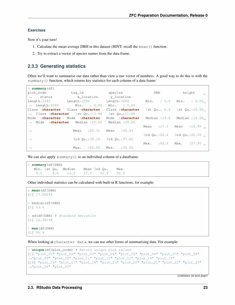
Often we’ll want to summarise our data rather than view a raw vector of numbers. A good way to do this is with thesummary() function, which returns key statistics for each column of a data frame:
> summary(df)plot_code tag_id species DBH height→˓ status x_location y_locationLength:3580 Length:3580 Length:3580 Min. : 5.0 Min. : 2.50→˓ Length:3580 Min. : 0.00 Min. : 0.00Class :character Class :character Class :character 1st Qu.: 8.4 1st Qu.:10.50→˓ Class :character 1st Qu.:12.68 1st Qu.:11.88Mode :character Mode :character Mode :character Median :13.6 Median :16.00→˓ Mode :character Median :25.40 Median :25.25
Mean :17.5 Mean :16.95→˓ Mean :25.31 Mean :25.04
3rd Qu.:22.4 3rd Qu.:22.00→˓ 3rd Qu.:38.10 3rd Qu.:37.80
Max. :92.9 Max. :57.50→˓ Max. :50.00 Max. :50.00
We can also apply summary() to an individual column of a dataframe:
> summary(df$DBH)Min. 1st Qu. Median Mean 3rd Qu. Max.5.0 8.4 13.6 17.5 22.4 92.9
Other individual statistics can be calculated with built-in R functions, for example:
> mean(df$DBH)[1] 17.50045
> median(df$DBH)[1] 13.6
> sd(df$DBH) # Standard deviation[1] 12.38198
> max(df$DBH)[1] 92.9
When looking at character data, we can use other forms of summarising data. For example:
> unique(df$plot_code) # Return unique plot values[1] "plot_01" "plot_02" "plot_03" "plot_04" "plot_05" "plot_06" "plot_07" "plot_08"→˓"plot_09" "plot_10" "plot_11" "plot_12" "plot_13" "plot_14" "plot_15"[16] "plot_16" "plot_17" "plot_18" "plot_19" "plot_20" "plot_21" "plot_22" "plot_23"→˓"plot_24" "plot_25"
(continues on next page)
2.3. RStudio Data Processing 23
ZFC Preparation Documentation, Release 0
(continued from previous page)
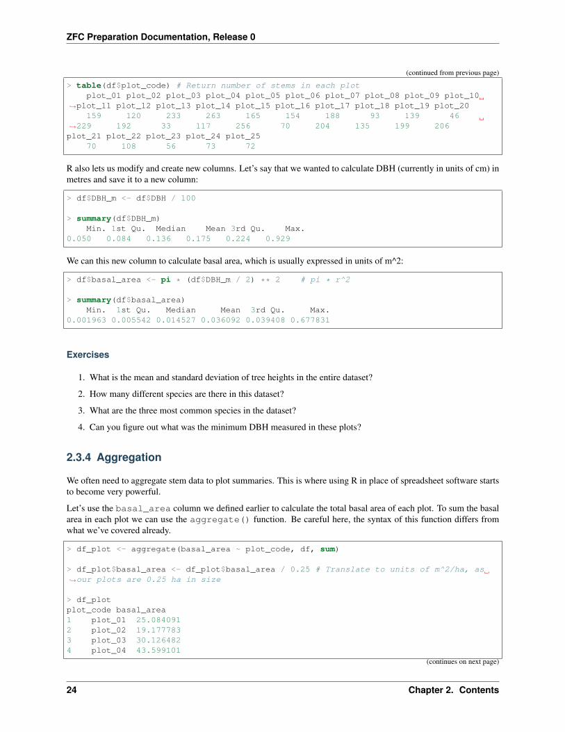
> table(df$plot_code) # Return number of stems in each plotplot_01 plot_02 plot_03 plot_04 plot_05 plot_06 plot_07 plot_08 plot_09 plot_10
→˓plot_11 plot_12 plot_13 plot_14 plot_15 plot_16 plot_17 plot_18 plot_19 plot_20159 120 233 263 165 154 188 93 139 46
→˓229 192 33 117 256 70 204 135 199 206plot_21 plot_22 plot_23 plot_24 plot_25
70 108 56 73 72
R also lets us modify and create new columns. Let’s say that we wanted to calculate DBH (currently in units of cm) inmetres and save it to a new column:
> df$DBH_m <- df$DBH / 100
> summary(df$DBH_m)Min. 1st Qu. Median Mean 3rd Qu. Max.
0.050 0.084 0.136 0.175 0.224 0.929
We can this new column to calculate basal area, which is usually expressed in units of m^2:
> df$basal_area <- pi * (df$DBH_m / 2) ** 2 # pi * r^2
> summary(df$basal_area)Min. 1st Qu. Median Mean 3rd Qu. Max.
0.001963 0.005542 0.014527 0.036092 0.039408 0.677831
Exercises
1. What is the mean and standard deviation of tree heights in the entire dataset?
2. How many different species are there in this dataset?
3. What are the three most common species in the dataset?
4. Can you figure out what was the minimum DBH measured in these plots?
2.3.4 Aggregation
We often need to aggregate stem data to plot summaries. This is where using R in place of spreadsheet software startsto become very powerful.
Let’s use the basal_area column we defined earlier to calculate the total basal area of each plot. To sum the basalarea in each plot we can use the aggregate() function. Be careful here, the syntax of this function differs fromwhat we’ve covered already.
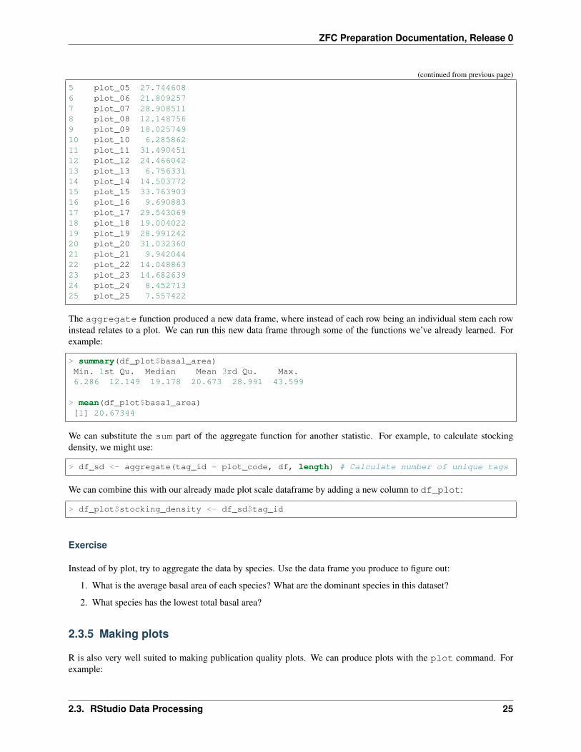
> df_plot <- aggregate(basal_area ~ plot_code, df, sum)
> df_plot$basal_area <- df_plot$basal_area / 0.25 # Translate to units of m^2/ha, as→˓our plots are 0.25 ha in size
> df_plotplot_code basal_area1 plot_01 25.0840912 plot_02 19.1777833 plot_03 30.1264824 plot_04 43.599101
(continues on next page)
24 Chapter 2. Contents
ZFC Preparation Documentation, Release 0
(continued from previous page)
5 plot_05 27.7446086 plot_06 21.8092577 plot_07 28.9085118 plot_08 12.1487569 plot_09 18.02574910 plot_10 6.28586211 plot_11 31.49045112 plot_12 24.46604213 plot_13 6.75633114 plot_14 14.50377215 plot_15 33.76390316 plot_16 9.69088317 plot_17 29.54306918 plot_18 19.00402219 plot_19 28.99124220 plot_20 31.03236021 plot_21 9.94204422 plot_22 14.04886323 plot_23 14.68263924 plot_24 8.45271325 plot_25 7.557422
The aggregate function produced a new data frame, where instead of each row being an individual stem each rowinstead relates to a plot. We can run this new data frame through some of the functions we’ve already learned. Forexample:
> summary(df_plot$basal_area)Min. 1st Qu. Median Mean 3rd Qu. Max.6.286 12.149 19.178 20.673 28.991 43.599
> mean(df_plot$basal_area)[1] 20.67344
We can substitute the sum part of the aggregate function for another statistic. For example, to calculate stockingdensity, we might use:
> df_sd <- aggregate(tag_id ~ plot_code, df, length) # Calculate number of unique tags
We can combine this with our already made plot scale dataframe by adding a new column to df_plot:
> df_plot$stocking_density <- df_sd$tag_id
Exercise
Instead of by plot, try to aggregate the data by species. Use the data frame you produce to figure out:
1. What is the average basal area of each species? What are the dominant species in this dataset?
2. What species has the lowest total basal area?
2.3.5 Making plots
R is also very well suited to making publication quality plots. We can produce plots with the plot command. Forexample:
2.3. RStudio Data Processing 25
ZFC Preparation Documentation, Release 0
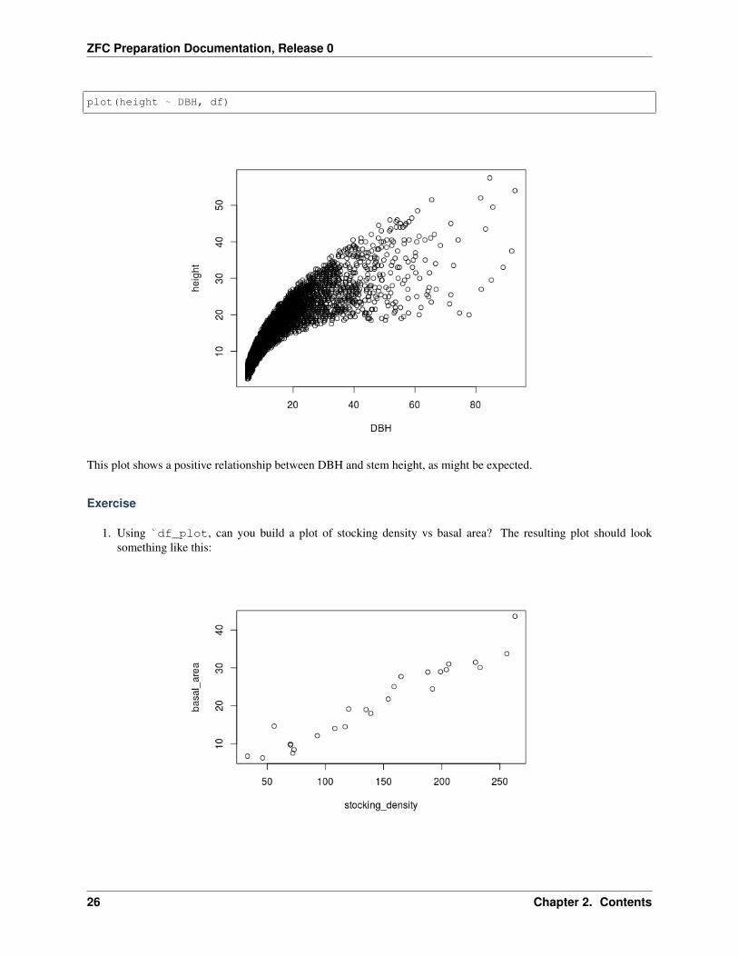
plot(height ~ DBH, df)
This plot shows a positive relationship between DBH and stem height, as might be expected.
Exercise
1. Using `df_plot, can you build a plot of stocking density vs basal area? The resulting plot should looksomething like this:
26 Chapter 2. Contents
ZFC Preparation Documentation, Release 0
2.3.6 Overview
Well done! Again, don’t worry if it didn’t all make sense, programming takes a long time to understand.
Here you’ve been introduced to data analysis in R. You should now understand:
1. How to load data into R (i.e. read.csv).
2. How to use and manipulate data frames (e.g. the $ operator).
3. How to generate summary statistics with data frams (e.g. summary).
4. How to aggreate data (i.e. aggregate).
5. How to make simple plots using data (i.e. plot).
2.3.7 Further reading
If you want to continue learning R, we can recommend the following resources:
1. https://www.datacamp.com/courses/free-introduction-to-r
2. https://www.youtube.com/playlist?list=PL6gx4Cwl9DGCzVMGCPi1kwvABu7eWv08P
3. https://ourcodingclub.github.io/
4. https://r4ds.had.co.nz/
Happy coding!
2.4 QGIS Setup
2.4.1 What is QGIS
QGIS is a desktop Geographic Information System (GIS) application that supports viewing, editing and analysis ofgeospatial data. QGIS is free and open source, and offers a viable alternative to commercial software such as ArcGIS.
2.4.2 Downloading QGIS
You can download QGIS from the QGIS website. Make sure you choose the correct version, which is Long termrelease, QGIS Standalone Installer for Windows. Most users will require the 64-bit version, but if you’re have anolder laptop you might need to download the 32-bit version.
If you’re struggling to find the correct version, you can also download it (Windows, 64-bit) directly here (392 MB).
Note: Are you using Linux or Mac, you may need to download a different version to that above. If accessing thislarge volume of data is a problem, we’ll bring along copies of QGIS to the workshop for you to install.
2.4.3 Installing QGIS
Once the download is complete, navigate to your Downloads folder, and run the executable namedQGIS-OSGeo4W-2.18.28-1-Setup-x86_64.exe (or similar).
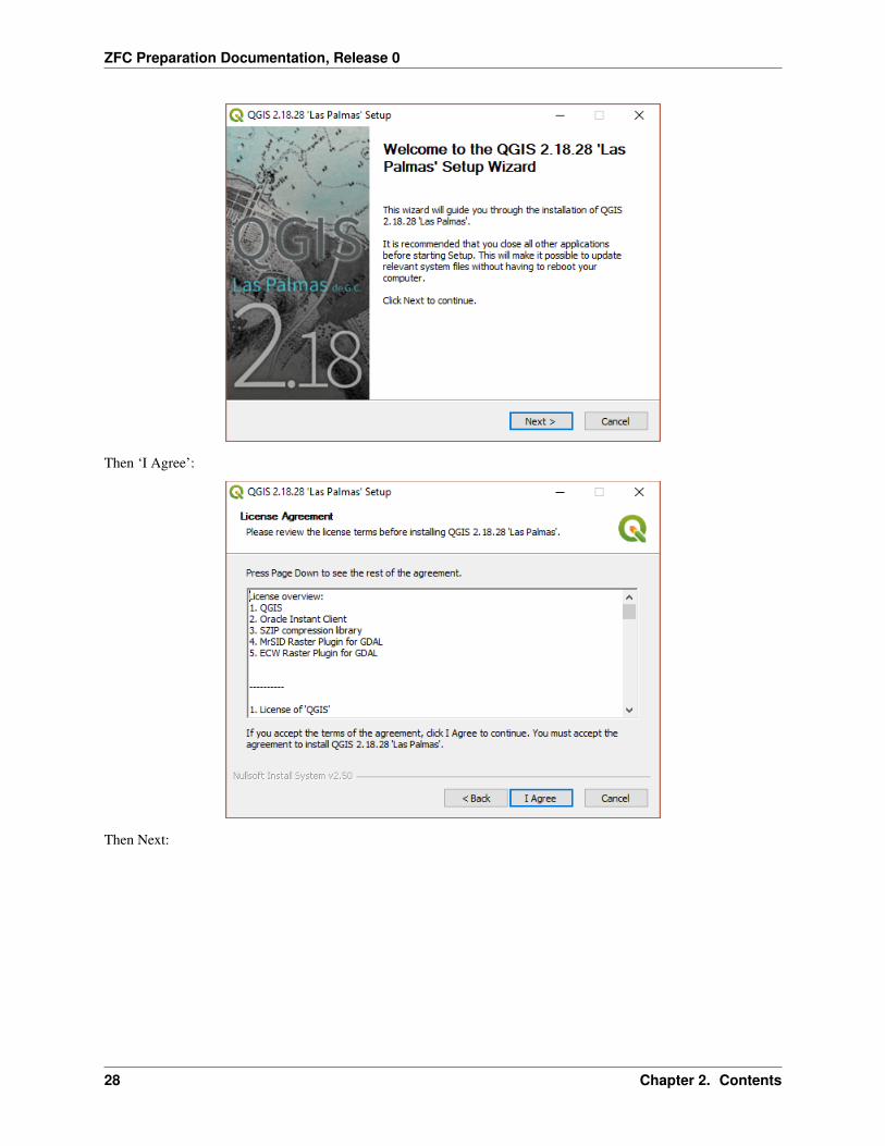
This will open the QGIS installer. You can accept all default settings. Click Next:
2.4. QGIS Setup 27
ZFC Preparation Documentation, Release 0
Then ‘I Agree’:
Then Next:
28 Chapter 2. Contents
ZFC Preparation Documentation, Release 0
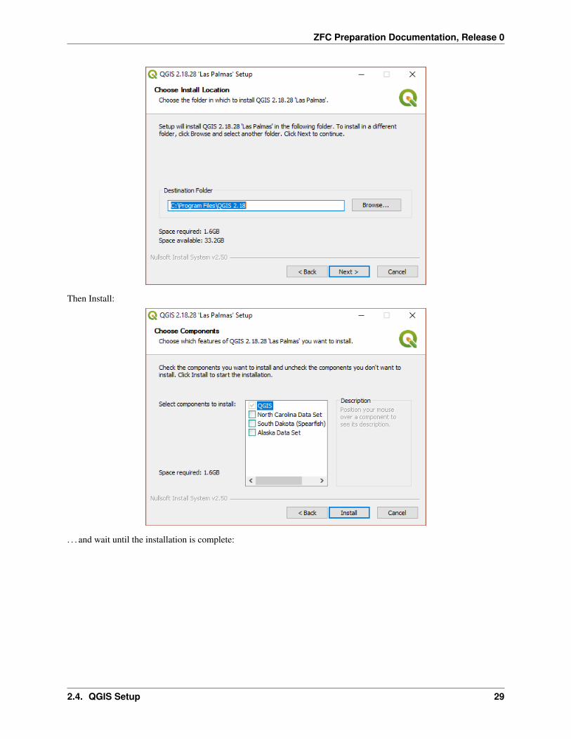
Then Install:
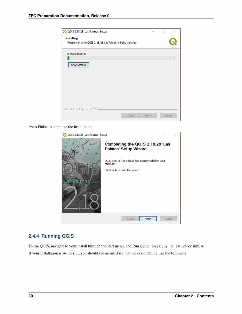
. . . and wait until the installation is complete:
2.4. QGIS Setup 29
ZFC Preparation Documentation, Release 0
Press Finish to complete the installation.
2.4.4 Running QGIS
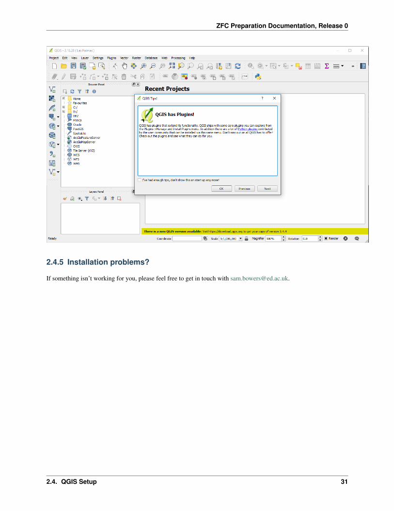
To run QGIS, navigate to your install through the start menu, and Run QGIS Desktop 2.18.28 or similar.
If your installation is successful, you should see an interface that looks something like the following:
30 Chapter 2. Contents
ZFC Preparation Documentation, Release 0
2.4.5 Installation problems?
If something isn’t working for you, please feel free to get in touch with [email protected].
2.4. QGIS Setup 31
ZFC Preparation Documentation, Release 0
32 Chapter 2. Contents
CHAPTER 3
Requirements
1. A Windows PC. Preferably a laptop that can be brought along to the workshop.
2. An internet connection suitable for downloading moderately large files (~100s MB).
3. A sense of adventure!
33
ZFC Preparation Documentation, Release 0
34 Chapter 3. Requirements

CHAPTER 4
Contact
If you encounter problems or need any assitance, please feel free to email Sam Bowers at [email protected].
35