Zhang weglein-2008

Direct non-linear inversion of 1D acoustic media using inverse scatteringsubseries

H. Zhang†and A B. Weglein†Presently at ConocoPhillips

Abstract

A task specific multi-parameter 1 direct non-linear inversion subseries of the inverse scatteringseries is derived and tested for a velocity and density varying 1D acoustic medium. There arevarious linear estimate solutions in the literature ( e.g., Raz, 1981, Clayton and Stolt, 1981, Stoltand Weglein, 1985) that assume an adequate estimate of medium properties above any giventarget reflector. However, this is the first seismic inversion method that: (1) neither assumesnor requires an adequate estimate of medium properties above any reflector, and (2) does notassume that the changes in physical properties satisfies a linear relationship to the reflection dataat the target, and (3) the most importantly the method stands alone in being a direct inversion.The meaning of direct is that there are formulas that explicitly solve for and directly outputthese physical properties, without e.g., search algorithms and optimization schemes, and proxiesthat typically characterize indirect methods. Numerical test results indicate that one termbeyond linear provides added value beyond standard linear techniques and common practice forestimating changes in physical properties at a target. Imaging and inversion for a two parametermedium directly in terms of data and reference properties is much more complicated than that ofthe one parameter case. The message delivered from this study extends and progresses beyondthe earlier one communicated in a one parameter velocity only medium, and serves as a necessaryand critical step in, and guide for, the development of the yet more complicated and realisticelastic isotropic direct depth imaging and non-linear parameter estimation. Three importantissues are identified and/or further progressed within the multi-parameter acoustic context andscope of this paper: (1) the concept of purposeful perturbation, (2) how the inverse seriesaddresses the phenomena in linear inversion known as leakage, and (3) special parameter forlinear inversion that is immune to linear inversion leakage, and the very significant implication ofthe latter result for direct depth imaging without the velocity model, are presented and discussedby analyzing these new two parameter non-linear direct inversion formulas and methods.

Introduction

The objective of seismic exploration is to determine the location (imaging) and mechanical proper-ties (inversion) of subsurface targets to identify hydrocarbon resources in the earth using recordeddata. The inverse scattering series has a tremendous generality and comprehensiveness allow-ing many distinct traditional processing objectives to be achieved within a single framework, butwithout the traditional need to provide information about the properties that govern actual wavepropagation in the earth. It begins with scattering theory, which is the relationship between the

1Within the context and scope of this paper, a multi-parameter medium is an acoustic medium where the velocityand/or density can vary.

184

Direct non-linear inversion of 1D acoustic media using inverse scattering subseries MOSRP07

perturbation or alteration in a medium’s properties and the concomitant perturbation or changein the wave field. The relationship between those two changes is always non-linear. Any changein a medium will result in a change in the wave-field that is non-linearly related to that physicalproperty change.

In this paper we examine the relationship between the perturbation in a medium and the pertur-bation in a wave field for the case of a 1D variable velocity and variable density acoustic medium.We assume the original unperturbed medium is a homogeneous whole-space. We further assumethat free surface and internal multiples have been removed (see, e.g., Weglein et al., 2003). Andwe assume that we are recording primaries, and our objectives are to: (1) locate reflectors and (2)determine medium properties of the actual medium. In this paper we present: (1) the first deriva-tion of equations to directly achieve those two distinct objectives for a one dimensional velocity anddensity varying acoustic medium, and (2) we then reduce this general formalism to the special caseof a single horizontal reflector, where the acoustic medium above the reflector is known, but theobjective is to determine the acoustic properties of the half-space below the reflector. For the lattersingle reflector case, the recorded data have a non-linear relationship with the property changesacross this reflector. Current inversion methods include: (1) the linear approximation (e.g., Claytonand Stolt, 1981; Weglein and Stolt, 1992) which is often useful, especially in the presence of smallearth property changes across the boundary and/or small angle reflections, and (2) indirect modelmatching methods with global searching (e.g., Tarantola et al., 1984; Sen and Stoffa, 1995) whichdefine an objective function assumed to be minimized when the best fitting model is obtained.The assumptions of the former methods (like the small contrast assumptions) are often violated inpractice and can cause erroneous predictions; the latter category usually involves a significant andoften daunting computation effort (especially in multi-D cases) and/or sometimes have reportederroneous or ambiguous results.

In this paper, a more comprehensive multi-parameter multi-dimensional direct non-linear inversionframework is developed based on the inverse scattering task-specific subseries (see, e.g., Wegleinet al., 2003). In order to provide more accurate and reliable target identification especially withlarge contrast, large angle target geometry, we isolated the inverse scattering subseries responsiblefor non-linear amplitude inversion of data.

The original inverse scattering series research aimed at separating imaging and inversion tasks onprimaries was developed for a 1D acoustic one parameter case (constant density medium, onlyvelocity variable in depth) and a plane wave at normal incidence (Weglein et al., 2002; Shaw et al.,2003). In this paper we move a step closer to seismic exploration relevance by extending that earlierwork to a multi-parameter case — two parameter case (velocity and density vary vertically in depth)and allowing for point sources and receivers over a 1D acoustic medium. Clayton and Stolt (1981)gave a two parameter linear inversion solution for 2D acoustic media (velocity and density varyboth vertically and laterally). In this paper, we use the same parameters but concentrate on 1Dacoustic media to derive the direct non-linear inversion solution. In the application of the directnon-linear inverse algorithm, we move one step each time (e.g., from one parameter 1D acousticcase to two parameter 1D acoustic case, or to one parameter 2D acoustic case, instead of ‘jumping’directly to two parameter 2D acoustic case) so that we can solve the problem step by step andlearn lessons from each step which would guide us to step further towards our goal of greater

185


realism and increased reliable prediction. For one parameter 1D and 2D acoustic media, some workon direct non-linear imaging with reference velocity is presented by Shaw (2005) and Liu et al.(2005). It has been shown in this paper that imaging and inversion for two parameter mediumare much more complicated compared to one parameter case, although it seems like just simplyadding one parameter. Examples of the new inverse issues that arise in a two parameter world (andneeded responses) that have no one parameter analogue are leakage, purposeful perturbation forthat issue, and the identification of the special parameter for inversion that avoids leakage, and theconceptual insights that this understanding provides for our campaign to address pressing imagingand inversion challenges.

For the direct non-linear inversion solution obtained in this paper, the tasks for imaging-only andinversion-only terms are separated. Tests with analytic data indicate significant added value forparameter predictions, beyond linear estimates, in terms of both the proximity to actual value andthe increased range of angles over which the improved estimates are useful.

A closed form of the inversion terms for the one-interface case is also obtained. This closed formmight be useful in predicting the precritical data using the postcritical data.

A special parameter ∆c (∆c = c−c0) (P-wave velocity change across an interface) is also found. ItsBorn inversion (∆c)1 always has the right sign. That is, the sign of (∆c)1 is always the same as thatof ∆c. In practice, it could be very useful to know whether the velocity increases or decreases acrossthe interface. After changing parameters, from α (relative changes in P-wave bulk modulus) and β(relative changes in density) to velocity and β, another form of the non-linear solution is obtained.There is no leakage correction (please see details in the section on three important messages) inthis solution. This new form clearly indicates that the imaging terms care only about velocityerrors. The mislocation is due to the wrong velocity. This is suggestive of possible generalizationto multi-D medium, and also of possible model-type independent imaging which only depends onvelocity changes.

The following section is a brief introduction of the inverse scattering subseries. We then gave theone dimensional multi-parameter acoustic derivation in detail, and that is followed by the numericaltests for the single reflector case. We also provided a further discussion about the special physicalnon-leaking acoustic parameter.

Inverse scattering subseries

Scattering theory relates the perturbation (the difference between the reference and actual mediumproperties) to the scattered wave field (the difference between the reference medium’s and theactual medium’s wave field). It is therefore reasonable that in discussing scattering theory, webegin with the basic wave equations governing the wave propagation in the actual and referencemedium, respectively 2,

LG = δ, (1)2In this introductory math development, we follow closely Weglein et al. (1997); Weglein et al. (2002); Weglein

et al. (2003).

186


L0G0 = δ, (2)

where L and L0 are respectively the differential operators that describe wave propagation in theactual and reference medium, and G and G0 are the corresponding Green’s operators. The δ onthe right hand side of both equations is a Dirac delta operator and represents an impulsive source.

The perturbation is defined as V = L0 − L. The Lippmann-Schwinger equation,

G = G0 +G0V G, (3)

relates G,G0 and V (see, e.g., Taylor, 1972). Iterating this equation back into itself generates theforward scattering series

G = G0 +G0V G0 +G0V G0V G0 + · · · . (4)

Then the scattered field ψs ≡ G−G0 can be written as

ψs = G0V G0 +G0V G0V G0 + · · ·= (ψs)1 + (ψs)2 + · · · , (5)

where (ψs)n is the portion of ψs that is nth order in V . The measured values of ψs are the data,D, where

D = (ψs)ms = (ψs)on the measurement surface.

In the inverse scattering series, expanding V as a series in orders of D,

V = V1 + V2 + V3 + · · · , (6)

where the subscript “i” in Vi (i=1, 2, 3, ...) denotes the portion of V i-th order in the data.Substituting Eq. (6) into Eq. (5), and evaluating Eq. (5) on the measurement surface yields

D = [G0(V1 + V2 + · · · )G0]ms + [G0(V1 + V2 + · · · )G0(V1 + V2 + · · · )G0]ms + · · · . (7)

Setting terms of equal order in the data equal, leads to the equations that determine V1, V2, . . .directly from D and G0.

D = [G0V1G0]ms, (8)

0 = [G0V2G0]ms + [G0V1G0V1G0]ms, (9)

0 =[G0V3G0]ms + [G0V1G0V2G0]ms + [G0V2G0V1G0]ms+ [G0V1G0V1G0V1G0]ms, (10)

etc. Equations (8) ∼ (10) permit the sequential calculation of V1, V2, . . ., and, hence, achievefull inversion for V (see Eq. 6) from the recorded data D and the reference wave field (i.e., theGreen’s operator of the reference medium) G0. Therefore, the inverse scattering series is a multi-D inversion procedure that directly determines physical properties using only reflection data andreference medium information.

187


Derivation of α1, β1 and α2, β2

In this section, we will consider a 1D acoustic two parameter earth model (e.g. bulk modulus anddensity or velocity and density). We start with the 3D acoustic wave equations in the actual andreference medium (Clayton and Stolt, 1981; Weglein et al., 1997)[

ω2

K(r)+∇ · 1

ρ(r)∇]G(r, rs;ω) = δ(r− rs), (11)

[ω2

K0(r)+∇ · 1

ρ0(r)∇]G0(r, rs;ω) = δ(r− rs), (12)

where G(r, rs;ω) and G0(r, rs;ω) are respectively the free-space causal Green’s functions thatdescribe wave propagation in the actual and reference medium. K = c2ρ, is P-wave bulk modulus,c is P-wave velocity and ρ is the density. The quantities with subscript “0” are for the referencemedium, and those without the subscript are for the actual medium. The perturbation is

V = L0 − L =ω2α

K0+∇ · β

ρ0∇, (13)

where α = 1− K0K and β = 1− ρ0

ρ are the two parameters we choose to do the inversion. Assumingboth ρ0 and c0 are constants, Eq. (12) becomes(

ω2

c20+∇2

)G0(r, rs;ω) = ρ0δ(r− rs). (14)

For the 1-D case, the perturbation V has the following form

V (z,∇) =ω2α(z)K0

+1ρ0β(z)

∂2

∂x2+

1ρ0

∂

∂zβ(z)

∂

∂z. (15)

V (z,∇), α(z) and β(z) can be expanded respectively as

V (z,∇) = V1(z,∇) + V2(z,∇) + · · · , (16)

α(z) = α1(z) + α2(z) + · · · , (17)

β(z) = β1(z) + β2(z) + · · · . (18)

Where the subscript “i” in Vi, αi and βi (i=1, 2, 3, ...) denote the portion of those quantities i-thorder in the data.Then we have

V1(z,∇) =ω2α1(z)K0

+1ρ0β1(z)

∂2

∂x2+

1ρ0

∂

∂zβ1(z)

∂

∂z, (19)

V2(z,∇) =ω2α2(z)K0

+1ρ0β2(z)

∂2

∂x2+

1ρ0

∂

∂zβ2(z)

∂

∂z, (20)

....

188


Substituting Eq. (19) into Eq. (8), we can get the linear solution for α1 and β1 in the frequencydomain

D(qg, θ, zg, zs) = −ρ0

4e−iqg(zs+zg)

[1

cos2 θα1(−2qg) + (1− tan2 θ)β1(−2qg)

], (21)

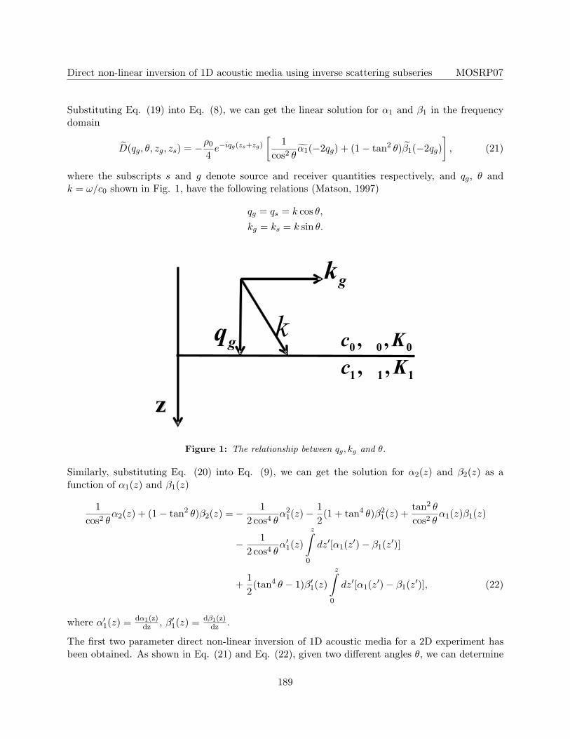
where the subscripts s and g denote source and receiver quantities respectively, and qg, θ andk = ω/c0 shown in Fig. 1, have the following relations (Matson, 1997)

qg = qs = k cos θ,kg = ks = k sin θ.

111 ,, Kc

gq k

gk

zz

000 ,, Kc

Figure 1: The relationship between qg, kg and θ.

Similarly, substituting Eq. (20) into Eq. (9), we can get the solution for α2(z) and β2(z) as afunction of α1(z) and β1(z)

1cos2 θ

α2(z) + (1− tan2 θ)β2(z) =− 12 cos4 θ

α21(z)−

12(1 + tan4 θ)β2

1(z) +tan2 θ

cos2 θα1(z)β1(z)

− 12 cos4 θ

α′1(z)

z∫0

dz′[α1(z′)− β1(z′)]

+12(tan4 θ − 1)β′1(z)

z∫0

dz′[α1(z′)− β1(z′)], (22)

where α′1(z) = dα1(z)dz , β′1(z) = dβ1(z)

dz .

The first two parameter direct non-linear inversion of 1D acoustic media for a 2D experiment hasbeen obtained. As shown in Eq. (21) and Eq. (22), given two different angles θ, we can determine

189


α1, β1 and then α2, β2. For a single-interface example, it can be shown that only the first threeterms on the right hand side contribute to parameter predictions, while the last two terms performimaging in depth since they will be zero after the integration across the interface (see the sectionon three important messages). Therefore, in this solution, the tasks for imaging-only and inversion-only terms are separated.

For the θ = 0 and constant density case, Eq. (22) reduces to the non-linear solution for 1D oneparameter normal incidence case (e.g., Shaw, 2005)

α2(z) = −12

α21(z) + α′1(z)

z∫−∞

dz′α1(z′)

. (23)

If another choice of free parameter other than θ (e.g., ω or kh) is selected, then the functionalform between the data and the first order perturbation Eq. (21) would change. Furthermore, therelationship between the first and second order perturbation Eq. (22) would, then, also be different,and new analysis would be required for the purpose of identifying specific task separated terms.Empirically, the choice of θ as free parameter (for a 1D medium) is particularly well suited forallowing a task separated identification of terms in the inverse series.

There are several important messages that exist in Eq. (21) and Eq. (22): (1) purposeful perturba-tion, (2) leakage, and (3) the special parameter for inversion. These three concepts will be discussedlater in this paper. In Eq. (21), it seems simple and straightforward to use data at two angles inorder to obtain α1 and β1. This is what we do in this paper. However, by doing this, it requires awhole new understanding of the definition of “the data”. That is part of the discoveries of on-goingresearch activities by Weglein et al. (2007). The imaging algorithm given by Liu et al. (2005) hasbeen generalized to the two parameter case by Weglein et al. (2007) based on the understandingof Eq. (22).

A special case: one-interface model

In this section, we derive a closed form for the inversion-only terms. From this closed form, we caneasily get the same inversion terms as those in Eqs. (21) and (22). We also show some numericaltests using analytic data. From the numerical results, we see how the corresponding non-linearterms contribute to the parameter predictions such as the relative changes in the P-wave bulkmodulus

(α = ∆K

K

), density

(β = ∆ρ

ρ

), impedance

(∆II

)and velocity

(∆cc

).

Closed form for the inversion terms

1. Incident angle not greater than critical angle, i.e. θ ≤ θc

For a single interface example, the reflection coefficient has the following form (Keys, 1989)

R(θ) =(ρ1/ρ0)(c1/c0)

√1− sin2 θ −

√1− (c21/c

20) sin2 θ

(ρ1/ρ0)(c1/c0)√

1− sin2 θ +√

1− (c21/c20) sin2 θ

. (24)

190


After adding 1 on both sides of Eq. (24), we can get

1 +R(θ) =2 cos θ

cos θ + (ρ0/ρ1)√(

c20/c21

)− sin2 θ

. (25)

Then, using the definitions of α = 1− K0K1

= 1− ρ0c20ρ1c21

and β = 1− ρ0ρ1

, Eq. (25) becomes

4R(θ)(1 +R(θ))2

=α

cos2 θ+ (1− tan2 θ)β − αβ

cos2 θ+ β2 tan2 θ, (26)

which is the closed form we derived for the one interface two parameter acoustic inversion-onlyterms.

2. Incident angle greater than critical angle, i.e. θ > θc

For θ > θc, Eq. (24) becomes

R(θ) =(ρ1/ρ0)(c1/c0)

√1− sin2 θ − i

√(c21/c

20) sin2 θ − 1

(ρ1/ρ0)(c1/c0)√

1− sin2 θ + i√

(c21/c20) sin2 θ − 1

. (27)

Then, Eq. (25) becomes

1 +R(θ) =2 cos θ

cos θ + i (ρ0/ρ1)√

sin2 θ −(c20/c

21

) , (28)

which leads to the same closed form as Eq. (26)

4R(θ)(1 +R(θ))2

=α

cos2 θ+ (1− tan2 θ)β − αβ

cos2 θ+ β2 tan2 θ.

As we see, this closed form is valid for all incident angles.

In addition, for normal incidence (θ = 0) and constant density (β = 0) media, the closed form Eq.(26) will be reduced to

α =4R

(1 +R)2. (29)

This represents the relationship between α and R for the one parameter 1D acoustic constantdensity medium and 1D normal incidence obtained in Innanen (2003). In this case, α becomes1− c20/c

21 and R becomes (c1 − c0) / (c1 + c0).

3. Derivation of the inversion terms from the closed form

From the closed form Eq. (26), using Taylor expansion on the left hand side

1(1 +R(θ))2

=[1−R(θ) +R2(θ)− . . .

]2,

191


and setting the terms of equal order in the data equal, we have

α1

cos2 θ+ (1− tan2 θ)β1 = 4R(θ), (30)

α2

cos2 θ+ (1− tan2 θ)β2 = −1

2α2

1

cos4 θ− 1

2(1 + tan4 θ)β2

1 +tan2 θ

cos2 θα1β1. (31)

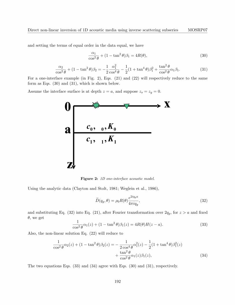
For a one-interface example (in Fig. 2), Eqs. (21) and (22) will respectively reduce to the sameform as Eqs. (30) and (31), which is shown below.

Assume the interface surface is at depth z = a, and suppose zs = zg = 0.

000 ,, Kc

111 ,, Kc

zz

xx

aa

00

Figure 2: 1D one-interface acoustic model.

Using the analytic data (Clayton and Stolt, 1981; Weglein et al., 1986),

D(qg, θ) = ρ0R(θ)e2iqga

4πiqg, (32)

and substituting Eq. (32) into Eq. (21), after Fourier transformation over 2qg, for z > a and fixedθ, we get

1cos2 θ

α1(z) + (1− tan2 θ)β1(z) = 4R(θ)H(z − a). (33)

Also, the non-linear solution Eq. (22) will reduce to

1cos2 θ

α2(z) + (1− tan2 θ)β2(z) =− 12 cos4 θ

α21(z)−

12(1 + tan4 θ)β2

1(z)

+tan2 θ

cos2 θα1(z)β1(z), (34)

The two equations Eqs. (33) and (34) agree with Eqs. (30) and (31), respectively.

192


Numerical tests

From Eq. (33), we choose two different angles to solve for α1 and β1

β1(θ1, θ2) = 4R(θ1) cos2 θ1 −R(θ2) cos2 θ2

cos(2θ1)− cos(2θ2), (35)

α1(θ1, θ2) = β1(θ1, θ2) + 4R(θ1)−R(θ2)

tan2 θ1 − tan2 θ2. (36)

Similarly, from Eq. (34), given two different angles we can solve for α2 and β2 in terms of α1 andβ1

β2(θ1, θ2) =[−1

2α2

1

(1

cos2 θ1− 1

cos2 θ2

)+ α1β1

(tan2 θ1 − tan2 θ2

)− 1

2β2

1

×(

cos2 θ1 − cos2 θ2 +sin4 θ1cos2 θ1

− sin4 θ2cos2 θ2

)]/ [cos(2θ1)− cos(2θ2)] , (37)

α2(θ1, θ2) =β2(θ1, θ2) +[−1

2α2

1

(1

cos4 θ1− 1

cos4 θ2

)+ α1β1

(tan2 θ1cos2 θ1

− tan2 θ2cos2 θ2

)−1

2β2

1

(tan4 θ1 − tan4 θ2

)]/(tan2 θ1 − tan2 θ2

); (38)

where α1 and β1 in Eqs. (37) and (38) denote α1(θ1, θ2) and β1(θ1, θ2), respectively.

For a specific model, ρ0 = 1.0g/cm3, ρ1 = 1.1g/cm3, c0 = 1500m/s and c1 = 1700m/s, in thefollowing figures we give the results for the relative changes in the P-wave bulk modulus

(α = ∆K

K

),

density(β = ∆ρ

ρ

), impedance

(∆II

)and velocity

(∆cc

)corresponding to different pairs of θ1 and

θ2.

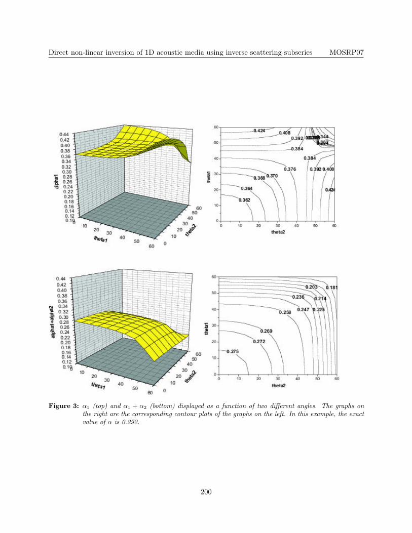
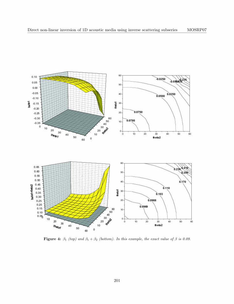
From Fig. 3, we can see that when we add α2 to α1, the result is much closer to the exact valueof α. Furthermore, the result is better behaved; i.e., the plot surface becomes flatter, over a largerrange of precritical angles. Similarly, as shown in Fig. 4, the results of β1 + β2 are much betterthan those of β1. In addition, the sign of β1 is wrong at some angles, while, the results for β1 + β2

always have the right sign. So after including β2, the sign of the density is corrected, which is veryimportant in the earth identification, and also the results of ∆I

I (see Fig. 5 ) and ∆cc (see Fig. 6)

are much closer to their exact values respectively compared to the linear results.

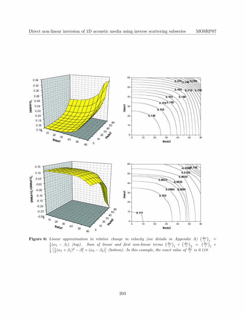
Especially, the values of(

∆cc

)1

are always greater than zero, that is, the sign of (∆c)1 is alwayspositive, which is the same as that of the exact value ∆c. We will further discuss this in the nextsection.

Three important messages

As mentioned before, in general, since the relationship between data and target property changesis non-linear, linear inversion will produce errors in target property prediction. When one actual

193


property change is zero, the linear prediction of the change can be non-zero. Also, when the actualchange is positive, the predicted linear approximation can be negative. There is a special parameterfor linear inversion of acoustic media, that never suffers the latter problem.

From Eq. (24) we can see that when c0 = c1, the reflection coefficient is independent of θ, thenfrom the linear form Eq. (36), we have(

∆cc

)1

=12(α1 − β1) = 0 when ∆c = 0,

i.e., when ∆c = 0, (∆c)1 = 0. This generalizes to (∆c)1 > 0 when ∆c > 0, or (∆c)1 < 0 when∆c < 0, as well. This can be shown mathematically (See Appendix B for details).

Therefore, we can, first, get the right sign of the relative change in P-wave velocity from the linearinversion (∆c)1, then, get more accurate values by including non-linear terms.

Another interesting point is that the image does not move when the velocity does not change acrossan interface, i.e., c0 = c1, since, in this situation, the integrands of imaging terms α1 − β1 in Eq.(22) are zero. We can see this more explicitly when we change the two parameters α and β to ∆c

cand β. Using the two relationships below (See details in Appendix A)(

∆cc

)1

=12(α1 − β1),

and (∆cc

)2

=12

[14(α1 + β1)2 − β2

1 + (α2 − β2)],

rewriting Eq. (22) as

1cos2 θ

(∆cc

)2

(z) + β2(z) =cos2 θ − 22 cos4 θ

(∆cc

)2

1

(z)− 12β2

1(z)

− 1cos4 θ

(∆cc

)′1

(z)

z∫0

dz′(

∆cc

)1

− 1cos2 θ

β′1(z)

z∫0

dz′(

∆cc

)1

. (39)

This equation indicates two important concepts. One is leakage: there is no leakage correction atall in this expression. Here the leakage means that, if the actual value of α (relative changes inP-wave bulk modulus) is zero, its linear approximation α1 could be non-zero since α and β arecoupled together (like the coupled term α1β1 in Eq. 22) and α1 could get leakage values from β1.While in Eq. (39), no such coupled term is present at all and thus, if the actual changes in thevelocity are zero, then its linear inversion

(∆cc

)1

would be zero and there would be no leakage fromβ1. This leakage issue or coupled term has no analogue in the 1D one parameter acoustic case(Eq. 23) since in this case we only have one parameter and there is no other parameter to leak

194


into. In other words, in the one parameter (velocity) case, each ‘jump’ in the amplitude of the data(primaries only) corresponds to each wrong location with a wrong amplitude for the parameterpredicted in the linear inverse step; while in the two parameter case of this paper, each ‘jump’ inthe data no longer has the simple one-to-one relationship with the amplitude and location of thetwo parameters.

The other concept is purposeful perturbation. The integrand(

∆cc

)1

of the imaging terms clearlytells that if we have the right velocity, the imaging terms will automatically be zero even withoutdoing any integration; otherwise, if we do not have the right velocity, these imaging terms wouldbe used to move the interface closer to the right location from the wrong location. The conclusionfrom this equation is that the depth imaging terms depend only on the velocity errors.

Conclusion

In this paper, we derive the first two parameter direct non-linear inversion solution for 1D acousticmedia with a 2D experiment. Numerical tests show that the terms beyond linearity in earthproperty identification subseries provide added value. Although the model we used in the numericaltests is simple, the potential within Eqs. (21) and (22) applies to more complex models since theinverse scattering series is a direct inversion procedure which inverts data directly without knowingthe specific properties above the target.

As shown above, adding one parameter in the wave equation makes the problem much more com-plicated in comparison with the one parameter case. Three important concepts (purposeful pertur-bation, leakage and special parameter for inversion) have been discussed and how they relate to thelinear and non-linear results for parameter estimation, addressing leakage, and imaging. Furtherprogress on these issues is being carried out with on-going research.

The work presented in this paper is an important step forward for imaging without the velocitymodel, and target identification for the minimally acceptable elastic isotropic target. In this paperfor the first time the general one-dimensional formalism for a depth varying acoustic medium ispresented for depth imaging and direct parameter estimation, without needing to determine mediumvelocity properties that govern actual wave propagation for depth imaging, or what medium is abovea target to be identified. The encouraging numerical results motivated us to move one step further— extension of our work to the isotropic elastic case (see, e.g., Boyse and Keller, 1986) using threeparameters. The companion and sequel paper to this one provides that extension.

Acknowledgements

We thank all sponsors of M-OSRP and we are grateful that Robert Keys and Douglas Foster forvaluable discussions.

195


Appendix A

In this appendix, we derive the expressions of(

∆cc

)1,(

∆cc

)2,(

∆II

)1

and(

∆II

)2

in terms of α1, β1

and α2, β2. Define ∆c = c− c0, ∆I = I − I0, ∆K = K −K0 and ∆ρ = ρ− ρ0.

Since K = c2ρ, then we have

(c−∆c)2 =K −∆Kρ−∆ρ

.

Divided by c2, the equation above will become

2(

∆cc

)−(

∆cc

)2

=∆KK − ∆ρ

ρ

1− ∆ρρ

.

Remember that α = ∆KK and β = ∆ρ

ρ , the equation above can be rewritten as

2(

∆cc

)−(

∆cc

)2

=α− β

1− β.

Then we have

2(

∆cc

)−(

∆cc

)2

= (α− β)(1 + β + β2 + · · · ), (40)

where the series expansion is valid for |β| < 1.

Similar to Eqs. (17) and (18), ∆cc can be expanded as(

∆cc

)=(

∆cc

)1

+(

∆cc

)2

+ · · · . (41)

Then substitute Eqs. (41), (17) and (18) into Eq. (40), and set those terms of equal order equalon both sides of Eq. (40), we can get (

∆cc

)1

=12(α1 − β1), (42)

and (∆cc

)2

=12

[14(α1 + β1)2 − β2

1 + (α2 − β2)]. (43)

Similarly, using I = cρ, we have

(I −∆I)2 = (K −∆K)(ρ−∆ρ).

Divided by I2, the equation above will become

2(

∆II

)−(

∆II

)2

= α+ β − αβ. (44)

196


Expanding ∆II as (

∆II

)=(

∆II

)1

+(

∆II

)2

+ · · · , (45)

and substitute Eqs. (45), (17) and (18) into Eq. (44), setting those terms of equal order equal onboth sides of Eq. (44), we can get (

∆II

)1

=12(α1 + β1), (46)

and (∆II

)2

=12

[14(α1 − β1)2 + (α2 + β2)

]. (47)

Appendix B

In this appendix, we show that(

∆cc

)1

has the same sign as ∆c. For the single interface example,from Eqs. (36) and (42), we have (

∆cc

)1

= 2R(θ1)−R(θ2)

tan2 θ1 − tan2 θ2.

The reflection coefficient is

R(θ) =(ρ1/ρ0)(c1/c0)

√1− sin2 θ −

√1− (c21/c

20) sin2 θ

(ρ1/ρ0)(c1/c0)√

1− sin2 θ +√

1− (c21/c20) sin2 θ

.

LetA(θ) = (ρ1/ρ0)(c1/c0)

√1− sin2 θ,

B(θ) =√

1− (c21/c20) sin2 θ.

ThenR(θ1)−R(θ2) = 2

A(θ1)B(θ2)−B(θ1)A(θ2)[A(θ1) +B(θ1)] [A(θ2) +B(θ2)]

,

where the denominator is greater than zero. The numerator is

2 [A(θ1)B(θ2)−B(θ1)A(θ2)] =2(ρ1/ρ0)(c1/c0)[√

1− sin2 θ1

√1− (c21/c

20) sin2 θ2

−√

1− sin2 θ2

√1− (c21/c

20) sin2 θ1

].

LetC =

√1− sin2 θ1

√1− (c21/c

20) sin2 θ2,

D =√

1− sin2 θ2

√1− (c21/c

20) sin2 θ1.

197


Then,

C2 −D2 =(c21c20− 1)

(sin2θ1 − sin2θ2).

When c1 > c0 and θ1 > θ2 , we have (Noticing that both C and D are positive.)(c21c20− 1)

(sin2θ1 − sin2θ2) > 0,

soR(θ1)−R(θ2) > 0;

Similarly, when c1 < c0 and θ1 > θ2 , we have(c21c20− 1)

(sin2θ1 − sin2θ2) < 0,

soR(θ1)−R(θ2) < 0.

Remembering that(

∆cc

)1

= 2 R(θ1)−R(θ2)tan2 θ1−tan2 θ2

. So for c1 > c0, (∆c)1 > 0 and for c1 < c0, (∆c)1 < 0 .

References

Boyse, W. E. and J. B. Keller. “Inverse elastic scattering in three dimensions.” J. Acoust. Soc.Am. 79 (1986): 215–218.

Clayton, R. W. and R. H. Stolt. “A Born-WKBJ inversion method for acoustic reflection data.”Geophysics 46 (1981): 1559–1567.

Innanen, Kristopher. A. Methods for the treatment of acoustic and absorptive/dispersive wave fieldmeasurements. PhD thesis, University of British Columbia, 2003.

Keys, R. G. “Polarity reversals in reflections from layered media.” Geophysics 54 (1989): 900–905.

Liu, F., A. B. Weglein K. A. Innanen, and B. G. Nita. “Extension of the non-linear depth imagingcapability of the inverse scattering series to multidimensional media: strategies and numericalresults.” 9th Ann. Cong. SBGf, Expanded Abstracts. . SBGf, 2005.

Matson, K. H. An inverse-scattering series method for attenuating elastic multiples from multi-component land and ocean bottom seismic data. PhD thesis, University of British Columbia,1997.

Raz, S. “Direct reconstruction of velocity and density profiles from scattered field data.” Geophysics46 (1981): 832–836.

Sen, M. and P. L. Stoffa. Global Optimization Methods in Geophysical Inversion. Amsterdam:Elsevier, 1995.

198


Shaw, S. A. An inverse scattering series algorithm for depth imaging of reflection data from alayered acoustic medium with an unknown velocity model. PhD thesis, University of Houston,2005.

Shaw, S. A., A. B. Weglein, D. J. Foster, K. H. Matson, and R. G. Keys. “Isolation of a leadingorder depth imaging series and analysis of its convergence properties.” M-OSRP Annual Report2 (2003): 157–195.

Stolt, R. H. and A. B. Weglein. “Migration and inversion of seismic data.” Geophysics 50 (1985):2458–2472.

Tarantola, A., A. Nercessian, and O. Gauthier. “Nonlinear Inversion of Seismic Reflection Data.”54rd Annual Internat. Mtg., Soc. Expl. Geophys., Expanded Abstracts. . Soc. Expl. Geophys.,1984. 645–649.

Taylor, J. R. Scattering theory: the quantum theory on nonrelativistic collisions. Wiley, New York,1972.

Weglein, A. B., F. V. Araujo, P. M. Carvalho, R. H. Stolt, K. H. Matson, R. T. Coates, D. Corrigan,D. J. Foster, S. A. Shaw, and H. Zhang. “Inverse scattering series and seismic exploration.”Inverse Problems 19 (2003): R27–R83.

Weglein, A. B., D. J. Foster, K. H. Matson, S. A. Shaw, P. M. Carvalho, and D. Corrigan. “Predict-ing the correct spatial location of reflectors without knowing or determining the precise mediumand wave velocity: initial concept, algorithm and analytic and numerical example.” Journal ofSeismic Exploration 10 (2002): 367–382.

Weglein, A. B., F. A. Gasparotto, P. M. Carvalho, and R. H. Stolt. “An inverse-scattering seriesmethod for attenuating multiples in seismic reflection data.” Geophysics 62 (1997): 1975–1989.

Weglein, A. B. and R. H. Stolt. 1992 “Approaches on linear and non-linear migration-inversion.”.Personal Communication.

Weglein, A. B., P. B. Violette, and T. H. Keho. “Using multiparameter Born theory to obtaincertain exact multiparameter inversion goals.” Geophysics 51 (1986): 1069–1074.

199


Figure 3: α1 (top) and α1 + α2 (bottom) displayed as a function of two different angles. The graphs onthe right are the corresponding contour plots of the graphs on the left. In this example, the exactvalue of α is 0.292.

200


Figure 4: β1 (top) and β1 + β2 (bottom). In this example, the exact value of β is 0.09.

201


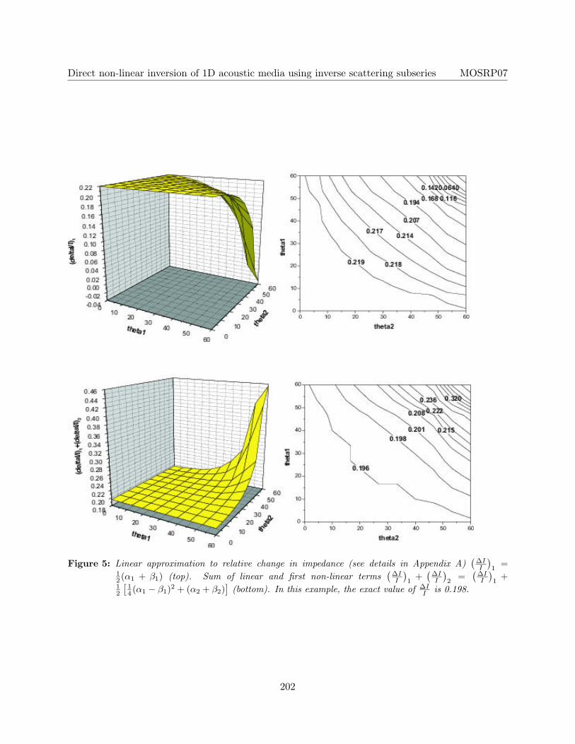
Figure 5: Linear approximation to relative change in impedance (see details in Appendix A)(

∆II

)1

=12 (α1 + β1) (top). Sum of linear and first non-linear terms

(∆II

)1

+(

∆II

)2

=(

∆II

)1

+12

[14 (α1 − β1)2 + (α2 + β2)

](bottom). In this example, the exact value of ∆I

I is 0.198.

202


Figure 6: Linear approximation to relative change in velocity (see details in Appendix A)(

∆cc

)1

=12 (α1 − β1) (top). Sum of linear and first non-linear terms

(∆cc

)1

+(

∆cc

)2

=(

∆cc

)1

+12

[14 (α1 + β1)2 − β2

1 + (α2 − β2)]

(bottom). In this example, the exact value of ∆cc is 0.118.

203

Documents

Zhang weglein-2008