Cost Pass Through and Welfare Effects of the Food Safety Modernization Act

Abstract

The Produce Rules of the Food Safety Modernization Act (FSMA) marked the first instance of the FDA directly regulating food safety activities at the farm-level. Since most fruits and vegetables were covered, the law’s comprehensive ‘across-the-board’ implementation potentially created offsetting cross-price effects on the demand side since most producers would be bearing the implementation costs simultaneously. However, the fixed costs nature of some other regulations costs, the different distribution of farm sizes across commodities and the potential for some commodities to be exempted suggest that the effects would vary across commodities.

We present an Equilibrium Displacement Model (EDM) to consider the effect of FSMA costs on prices and consumer and producer welfare. To parameterize the model, we use National Agricultural Statistics Service (NASS) and Food and Drug Administration (FDA) data to calculate the cost of implementing FSMA rules for 18 fruits and 21 vegetables, IRI storescan data to estimate demand elasticities, Agricultural Marketing Service data to calculate data wholesale costs shares, and supply elasticities from extant sources While varying across commodities, the average cost of implementing FSMA is 2.79 percent of farm revenue for fruits and 1.52 percent of farm revenue for vegetables, that farm prices increase by 1.68 percent (fruit) and 0.44 percent (vegetables), and that consumer prices increase by 0.70 percent (fruit) and 0.12 percent (vegetables). If there is no corresponding demand effect or cost saving at the farm level associated with the implementation of these regulations, farm welfare, as a percentage of revenue, falls by 1.11 percent (fruit) and 0.96 percent (vegetables). Also, we found that weak substitution patterns between commodities at the retail level caused off-setting cross-price effects to be weak.

Peyton Ferrier, Economic Research Service –USDA,Chen Zhen, University of Georgia, and

John Bovay, Economic Research Service - USDA

May 2016

*Selected Paper prepared for presentation for the 2016 Agricultural & Applied Economics Association annual meeting, Boston, MA, July 31-August 2

**Disclaimer: The views and opinions expressed in the paper are those of the authors and do not reflect those of the Economic Research Service or the United States Department of Agriculture.

1

I. Introduction

The 2011 passage of the Food Safety Modernization Act (FSMA) marked the most comprehensive legislative change to the authority of the Food and Drug Administration (FDA) to regulate food since the 1930s (Johnson, 2011, Johnson, 2014). Its passage empowered the FDA to impose new regulatory requirements on food producers and handlers, to expand requirements for and inspections of imports, and to issue mandatory recalls of food. For the first time, FDA maintained regulatory authority over production practices at the farm level. The latter set of regulations, collectively known as the Produce Safety Rule, is the focus of this article.

The Final Produce Safety Rule was published in November 2015, nearly three years after the Proposed Rule was first published for public comment. This rule mandates certain on-farm practices related to the safety of certain types of fresh produce. In particular, most farms covered by the regulations would have specific production practices regulated along five areas: agricultural water quality, biological soil amendments, worker health and hygiene, animal intrusion, and sanitary standards.1 Each of these practices is primarily oriented towards curtailing microbial contamination by limiting the main ways food is exposed to pathogens at the farm level.

The Produce Safety Rule only applies to raw agricultural commodities, and does not apply to a specific list of commodities that FDA deems to be rarely consumed raw, including asparagus, beets, and sweet corn. Additional exemptions include food grains (such as barley and wheat) and oilseeds (such as canola and soybean).

As part of the rulemaking process, FDA was required to estimate the total costs to industry of complying with each of the major rules (the Produce Safety Rule is one of several) and publish these estimates in Regulatory Impact Analyses (RIAs). In the RIA for the Produce Safety Rule, FDA used data from the 2012 Census of Agriculture to estimate the number of regulated farms in each of three size categories: $25,000 to $249,999 in annual sales;2 $250,000 to $499,999 in annual sales; and more than $500,000 in annual sales. Then, FDA estimated the costs of compliance for an average farm within each of these three size categories and aggregated costs across farms to estimate the total national cost of the regulation. The FDA estimates reveal that the costs of compliance with FSMA, as a share of revenue, are larger for smaller farms, because there are many fixed costs associated with the administrative and personnel components of the regulation and some associated with the food-safety process components. Table 1 summarizes FDA’s estimates of the cost of compliance by category of required practice.

There are several shortcomings to the FDA approach, and our analysis in this article provides a fuller sense of the distribution of costs of compliance with the FSMA Produce Safety Rule as well as estimating

1 Sprouts from beans and seeds, which have a greater tendency towards microbial contamination than other produce items, have additional, more rigorous requirements.2 Farms with less than $25,000 in annual sales of produce are exempt from the Produce Safety Rule.

2

market (equilibrium) effects. The same approach may also be used to simulate differences in the incidence of costs under FSMA by geographic region.

Each farming operation will have different costs of complying with the FSMA rule on produce safety based on differences in farm practices, local idiosyncrasies, and state laws. To give several examples, the quality of agricultural water varies tremendously. Some growers apply water directly to crops and treat the water first, while others apply water only to the roots of a tree. However, under the FSMA Produce Safety Rule, all agricultural water must meet the same stringent standards. Those producers who are currently treating their water before application to leafy greens may already be in compliance with the FSMA water requirements, while many orchards will have to incur substantial cost to treat water and meet that requirement. To give another example, California state law requires that farmworkers have access to toilets and hand-washing stations in the field (California Division of Industrial Relations, 2014), but this is not a requirement under Federal law—so growers in California will have an advantage in complying with this component of the rule. Wild animals are a hazard to food safety in some regions but are uncommon in other regions.3 So, even among fully regulated farms of the same size, costs of compliance with the rule on produce safety can vary greatly depending on region, crop grown, and food-safety practices adopted voluntarily. Our analysis does not address these inherent differences in the cost of complying with the Produce Safety Rule, but draws on the differences in compliance across farm size as given in the RIA.

By utilizing restricted-access data from the 2012 Census of Agriculture, we are able to simulate a fuller distribution of the costs of compliance with the FSMA Produce Safety Rule than the FDA does in its RIA. Because the vast majority of produce is grown on farms with more than $500,000 in annual sales, the distribution of costs among larger farms is particularly important. In addition, we estimate crop-specific distributions of farm sizes and costs of compliance with FSMA. The same approach could be also be applied to estimating differences in the cost of compliance with FSMA across geographic areas in the United States, but that aspect is not part of the current article.

<< Table 1 - Enumerated Costs of FSMA >>

II. Equilibrium Displacement Model (EDM)

An Equilibrium Displacement Model (EDM) allows for comparative static analysis of a market event across upstream and downstream elements of the supply chain. First, an initial market equilibrium is assumed to hold across the linked markets under consideration where supply and demand relationships are explicitly specified. Next, a reduced form of the model is derived, typically by translating key supply and demand relationships to more easily manipulated elasticity relationships. Then, a market shock, policy or restriction is simulated through the model to show how the equilibrium moves from its initial state to a new state after the shock. Finally, relevant welfare or policy metrics are developed which describe the event.

3 Growers generally make efforts to keep animals out of fields, not only because of food-safety concerns but also to prevent the animals from eating crops.

3

With our model, we assume that each retail food (Q ) requires two inputs in production – farm-level (unprocessed wholesale) food (X ) and marketing inputs (MI ). For instance, to sell an apple at the retail level, a grocery store purchases wholesale apples from farmers and marketing inputs (store space, shelving, cashiers, electricity, advertising, delivery trucks, etc.) We consider N goods within our model and the one-to-one correspondence allows N to index retail food (QN ), wholesale food (X N ),and the

specific marketing input requirement of retail food (MI N ). The prices of QN , XN , and MI N are denoted

respectively as PN ,W N , and PMIN with all of the aforementioned matrices being N ×1 in dimensions. The AN term captures any potential demand increase associated with food being safer for having adopted the FSMA mandated measures.

For retail food, we define the demand function as QND in (1) and the cost function as CN in (2), where

constant average costs is imposed for each good. Furthermore, if retail markets are competitive, price equals average cost, which implies the latter impression in (2). For wholesale foods, define the demand function as X N

D in (3) and the supply function as X NS in (3).4 As an input, wholesale food’s demand

function can be defined as the derivative of the retail food cost function in (2) with respect to W . The added costs of implementing FSMA regulations for wholesale producers is modeled as a percentage reduction in the prices farmers receive at the wholesale level. For example, if the cost of implementing FSMA regulations is 3.2% for pears, then farmers receive 96.8% of the prices paid (W ). For marketing

inputs, define the demand function as MI ND in (5) and the supply function as MI S in (6). Like the

demand for individual wholesale foods, the demand for marketing inputs is the derivative of the retail food cost function in (2) with respect to PMI . The supply of marketing depending solely on PMI . These equations are collectively:

(1) Retail Food Demand: QND=QN

D (PN , AN ),

(2) Retail Food Cost: Cn=cn (W n ,PMI )Qn → Pn=cn (W n , PMI ),

(3) Wholesale Food Demand: X nD=(∂cn (W n ,PMI )/∂W n )Qn=gn (W n ,PMI )Qn,

(4) Wholesale Food Supply: X nS=Xn

S (W n× (1−CS )n ),

(5) Marketing Input Demand: MI nD=(∂cn (W n, PMI )/∂ PMI )Qn=hn (W n ,PMI )Qn, and

(6) Marketing Input Supply: MI S=MI S (PMI )

Comparative Statics

Total differentiation of equations (1) through (6) allows the market equilibrium equations to be represented in terms of elasticities and cost shares in (1’) through (6’). Specifically, where ηN are the

4 For simplicity, we assume that the cross price elasticity of supply is zero for all goods.

4

Marshallian demand elasticities for retail food (Q ), γNare the Hicksian demand elasticities for the inputs (X ), γMI are the Hicksian demands for the marketing input (MI ), εN are the elasticities of wholesale food supply, and sN are cost share of X in the production of Q, we denote dl as the change in a variable’s log value so that dlP equals ∂ P/P, dlQ equals ∂Q /Q, and so on. As shown in the Appendix, these (1) through (6) can be rewritten as:

(1’) dlQ=∑k=1

N

ηnkdl Pn+α n

(2’) dl Pn=sndlW n+(1−sn)dlPMI

(3’) dl Xn=γ n ,ndlW n+γ n ,MIdlPMI+dlQ

(4’) dl Xn=εndlW n+εn log (1−CS )n

(5’) dl MI n=γMI ,ndlW n+γMI ,MI dlPMI+dlQ

(6’) dlPMI=(εMI )−1dl MI

Let βN be an N x 1 matrix with each element equaling βn=log (1−CSn ). For simplicity, we assume that α n is equal to zero. By totally differentiating equations (1) to (6), re-arranging terms as elasticities and budget shares, and assuming that the supply of marketing inputs is perfectly elastic, we can represent these relationships as (See the Appendix for details):

(1’’) dlQN−ηN dl PN=0

(2’’) dl PN−sN dlW N=0

(3’’) dl X N−γN dlWN−dlQN=0

(4’’) dl X N−εN dlW N=εN βN

(5’’) γN dlW n+dlQN−dlMI N=0

Additionally, as shown in the Appendix, γn and γmi can specified as −(1−sn )σMI and (1−sn )σmi where

σ is the elasticity of substitution between X N and MI for each QN. In matrix form, equations (1’’) through (5’’) are simply AZ=C where:

A=[ IN −ηN 0N0N IN 0N

0N−sN

0N0N

−I N 0N IN0N 0N IN

−I N 0N 0N

( IN−sN )σMI

−εN−( IN−sN )σMI

0N0NI N

], Z=[dlQN

dlPN

dlX N

dlW N

dlMI N], and C=[ 0

00

εN β N

0].

5

Each element in A is an N ×Nmatrix while each element in Z and C are N ×1. Table (1) provides a summary of the variable names and their descriptions. In our model, FSMA regulations causes the βterms to shift from 0 to log (1−CS )n. The solutions for Z are obtained as:

(7) Z=A−1C

The new market equilibrium of prices and quantities (Q1 ,P1 , X1 ,W 1 , MI 1 ) are fully specified by the

solution for Z and the initial values of prices and quantities (Q0 , P0 , X0,W 0 , MI 0 ).

Welfare Changes

The new calculated market equilibrium can be used to develop approximations of the changes to welfare of retail consumers(CSn ) and farm producers (PSn ). The assumption that markets are competitive and that price equals costs at the retail level fixes the retail surplus at the constant level of zero. Similarly, our assumption that the supply of marketing inputs is perfectly elastically supplied precludes the possibility of a marketing surplus supplier surplus. The general formulas for the producer and consumer surplus are:

(8) dCS n≈ (P0 , n×dlPn )× (Q0 , n× (1+0.5dlQn ))=P0 , nQ0 , n (dlPn× (1+0.5dlQn ))

(9) dPSn≈W 0 ,n× (dlW n−CS n )× (X 0 ,n× (1+0.5dlX n ))

dPSn=W 0 , n X0 ,n (dlW n−CS n+1+0.5dlXn )

Cumulatively across all goods, the consumer and producer surplus changes are:

(10) ∆CSN ≈∑NP0 , nQ0 , n×(dlPn×(1+ 12 dlQn))

∆CSN ≈ P0 , NQ0 , N∑Nwn×(dlPn×(1+ 12 dlQn))

(11) ∆ PSn≈∑NW 0 ,n X0 ,n (dlW n−CSn )(1+ 12 dlX n)

In (10), P0 , NQ0 , N are initial total consumer expenditure and wn are average consumer shares of that expenditure. Note that individual goods, the consumer and produce surplus changes can be expressed as a percentages of initial consumer expenditure (exp=P0 , nQ0 , n ) and initial seller revenue

(Rev=W 0 ,n X0 ,n ) respectively as:

(12) ∆CS /exp≈−dlPn×(1+ 12 dlQn)

6

(13) ∆ FS /Rev ≈ (dlW n−CSn )(1+ 12 dlXn)Cost Pass Through

The initial cost shift for an individual goods is borne by both farm producers and retail consumers. In response to the cost shift increase, the percentage of that price increase transmitted to consumer prices and farm prices are CPT and FPT , or:

(14) CPT n≈dlPn/CSn

(15) FPT n≈dlW n/CS n

Typically, CPTwill be smaller than FPT as the potential of consumer substitution away from a good further mutes the initial price change. However, in some cases, substitution effects may potential cause demand substitution to a particular good if it is a strong substitute for other goods at the consumer level. In this case, economic theory does not preclude CPT being greater than FPT .

Valuing Exemptions and Measuring the Cost of Unilateral Implementation

To measure the value of an exemptions for an individual good, one adjusts the β matrix to reflect that exempt good faces no cost shift while other commodities face the cost shift caused by the FSMA regulations. For example, to consider the value of the 2ndvegetable commodity being exempted, one can calculate the welfare change associated with β2ndExempt as below:

(16) ExVal2=∆ PS2 (β2ndExempt ) where β2ndExempt=[log (1−CS 1)log (1 )

log (1−CS3 )⋮

log (1−CSN )]

If similar fresh fruits and vegetables are substitutes, then the value of the exemption, in terms of the change in producer surplus, will exceed the savings in costs associated with compliance. FSMA regulations on substitute commodities causes their prices to rise and thereby increasing the demand for the exempt commodities.

Denote the value of comprehensively enacting FSMA regulations rather than having those regulation applied to individual commodities as VCE. This value is the (absolute value of) the difference between the loss under unilateral enactment and comprehensive enactment. For example, the value of comprehensively imposing the FSMA regulations unilaterally on commodity 2 is:

7

(17) VCE2=−(∆ PS2 ( β2ndOnly )−∆ PS2 (β All)) where β2ndOnly=[log (1 )

log (1−CS2 )log (1 )⋮

log (1 )]

III. Data

Cost Shifts

As described earlier, to estimate the cost of implementing FSMA regulation for each commodity (the CS variable), we combine data on the distribution of farm sizes in the 2012 Census of Agriculture from the National Agricultural Statistics Service with data published in the Food and Drug Administration’s Regulatory Impact Analysis (RIA) on the final cost of implementing FSMA regulations. According to the RIA, costs varied with farm size for reasons such as the number of workers that required training and the cost of bookkeeping. Most strikingly, the large fixed costs of the regulations created substantial economics of scale in their implementation. Across all farm size, FSMA costs represented 1.53percent of the farm’s total sales revenue. For large farms, however, this percentage was only 0.88 percent while for small and very small farms it was 6.03 and 6.79 percent.

The RIA did not specifically disaggregate the cost of implementing FSMA across commodities. For farms surveyed, NASS data – the primary data source on the production composition of U.S. farms – provides detailed statistics on the planted acreage of each commodity, including some distinctions for whether goods are destined for further processing. Farm sales, however, are only reported for aggregate categories such as fruit, vegetable, and berry sales. These values allow us to assign a farm-level FSMA-implementation cost per unit of sales. Because farms with more than one type of produce crop are relatively common and yields per planted acre vary greatly, the share of farm sales attributable to individual goods is not readily observable and further defining the farm cost of implementing FSMA by commodity requires further assumptions.

We compute an average cost of implementing FSMA by commodity as follows. First, we compute average cost of implementing FSMA rules for each of the farms in the NASS Ag Census data. We use the FDA estimate of the recurring cost of compliance per farm upon full implementation of FSMA, for each of three size categories described earlier. In addition, we extrapolate (from FDA’s line-item costs) the cost of compliance for the smallest conceivable regulated farm: one with $25,000 in sales, one acre, and one employee. We develop a linear interpolation of costs for all farms with other sales values in the interval between $25,000 and $3,450,000—the FDA’s estimate of the average sales value for farms with at least $500,000 in sales. For farms with more than $3,450,000, we assume that the marginal cost of compliance with respect to sales is zero.

Second, we calculate each farm’s share of the total acreage planted acres for each of the commodities we consider. Third, we multiply each farm’s acreage shares for each commodity by that farm’s cost of implementing FSMA as a percentage of sales. Because, in our model, implementation cost is a function

8

of farm size, this method will make our estimated cost of implementing FSMA higher for crops that are produced on smaller farms while also accounting for the possibility of mixed production farms. If a mixed production farm maintains only a trivial acreage of a given commodity, then its contribution to that commodity’s average implementation costs will be similarly small.5

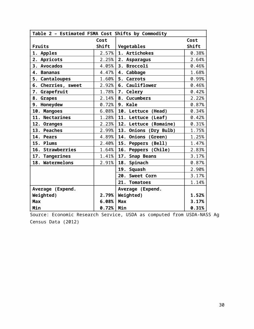
Estimates of the cost of implementing FSMA using this method are provided in Table 2. Figures 1 and 2 show these estimates graphically. The high implementation costs for bananas and mangoes are likely a data anomaly attributable to the very small scale of domestic production for these primarily imported goods. Aside from those goods, implementation costs range from 0.72 to 4.89 percent with 2.79 percent being the average for fruits and from 0.31 to 3.17 percent with 1.52 percent being the average for vegetables.

<< Table 2 - The Cost of Implementing FSMA Regulations by Commodity >>

<< Figure 1 – The Cost of Implementing FSMA by Farm Size (Fruits) >>

<< Figure 2 – The Cost of Implementing FSMA by Farm Size (Vegetables) >>

Figures 1 and 2 show the differences in implementation costs for commodities disaggregated by size. Again, the dominant driver in our calculations is the size of the farm as measured by total sales6.

Cost Shares and Supply Parameters

To estimate the share of the retail commodity’s costs that is derived from the cost of wholesale agricultural costs, we divide the wholesale price by the retail price index. We obtain wholesale prices from the USDA’s Agricultural Marketing Service while retail prices are calculated as a weighted average of observed prices within our IRI InfoScan retail scanner dataset. Table 3 provides estimates of these cost shares. In general, our share are higher than those found by Stewart (2006). By construction, the share of the retail price attributable to marketing inputs is the residual share (1−sn ) in our two-input production function.

To parameterize the supply relationships with our model we relied on the extant literature to provide the elasticity of supply relationships and the elasticity of substitution which we present in Table 3 as well. In general, this literature has several limitations. First, supply response varies with the time frame which is considered. Over shorter market time periods, supply is less elastic with regard to price. A typical framework for estimating supply response is to use lagged seasonal or annual prices to form an

5 Importantly, this method only addresses farm size as source of variation in the cost of implementing FSMA and should be interpreted with the understanding that data is unavailable to determine a more specific cost estimate. Aside from size, differences in yields will affect the weighting of each farm’s share weighting to the average cost of implementation by commodity. Implementation costs will be lower for different for types, especially if farms have already undertaken food safety investment prior to FSMA being developed. Farm costs to implementing FSMA will likely differ in their labor usage and specific costs will likely vary regionally. Some smaller farms may be exempt from implementing FSMA farms because the sell products locally or directly to consumers.6 Two important factors are not currently incorporated into these estimates. First, imports are assumed to have the same implementation costs as domestic producers. Second, existing investments in food safety equipment and practices are not broken out by commodity.

9

expectation of future prices based on some autoregressive regression structure. Then, this relationship can be used to determine the amount that supply changes in response to a change in the expected average price both in the short run and the long-run. Across studies however, the time frame for response may not be the same. At the same time, supplies of orchard crops (and other crops requiring an established root stock) will be far less responsive to short run price changes (elastic) than crops replanted annually.

Second, with regard to the elastic of substitution between agricultural commodity production and marketing inputs, to our knowledge, only Wohlgenant (1989) has systematically estimated this value and only for vegetables as a broad aggregate category. Instead, studies (Okrent and Alston, 2012) often assume that marketing inputs and wholesale commodities are used in fixed proportions which implies that the elasticity of substitution is zero. Besides making the models tractable, the fixed proportions assumption is intuitively appealing – selling one retail apple require one wholesale apple as an input. However, fixed proportions in production is a limiting case, however, and any departure from it (σ>0 ) will tend to make the wholesale demand for the commodity more elastic and dampen the retail-level price increase of a FSMA cost shift. As indicated in Table 3, we assumed the elasticity of substitution (σ ) was 0.54 for all vegetables and 0 for all fruits.

Table 3 listed the price elasticity of supply used within the EDM. These values range from between 0.05 and 0.905 for fruits and 0.097 and 1.19 for vegetables. We assume that all the cross-price elasticities of supply are zero so that all the off-diagonal elements of εN are zero.

<< Table 3 – Elasticities of Supply and Substitution >>.

In certain estimates given in Table 3 we interpolated the supply elasticity estimate based on the values for similar crops. In future work, we will include sensitivity tests for small changes in our supply elasticity values to test the significance of the specification.

Demand Model

We use IRI InfoScan retail scanner data to estimate the elasticities of demand for goods in our model using a two-stage budgeting model. In the first stage, consumers allocates total expenditures between the fruit group, the vegetable group, and a numéraire good. In the second stage, consumers allocate expenditures across 18 fruit categories and 21 vegetable categories for expenditure in their respective subcategories. In each stage, we choose the quadratic almost ideal demand (QUAID) (Banks, et al., 1997) as the demand function.

Compared with the almost ideal demand system (AIDS), the QUAID system has more flexible Engel curves but retains the exact aggregation property of AIDS so that market-level data can be used to make inferences about consumer behavior. The conditional budget share equation within the fruit group is

(18) wmit=αmit+∑j=1

n

γij ln pmit+ βi ln [ xmta ( pmt ) ]+ λi

b ( pmt ) [ ln [ xmta ( pmt ) ]]

2

10

where wmit is the expenditure share of fruit category i in market m and time t , pmit is the price index of category j , n is the number of fruit categories within the group; xmt is total fruit expenditure, and

α , γ , β , and λ are parameters. The a ( pt ) and b ( pt ) terms are defined as:

ln a ( pmt )=α0+∑i=1

n

αi0 ln pmit+0.5∑i=1

n

∑j=1

n

γ ij ln pmit ln pmjt

and

b ( pmt )=∏i=1

n

pmitβ i ,

respectively. We assume the intercept αmit to be a linear function of market and seasonal fixed effects

(19) αmit=αi0+∑l=2

72

α ilmktml+∑r=2

13

αir sea tr ,

where mktml and seatr are dummy variables for market l and the rth time period within a year.

Fruit and vegetable sales data come from the IRI InfoScan retail scanner data that the USDA Economic Research Service acquired to support its food market and policy research. Our sample covers 65 quadweeks (i.e., 4-weekly periods) between January 6, 2008 and December 29, 2012. In InfoScan, there are 65 markets and 8 standard whitespaces (i.e., remaining areas). We dropped the Green Bay, WI market from the sample due to insufficient retail data for the study period. This gives a balanced panel dataset with 4,680 market-quadweek observations. The InfoScan dataset at ERS contains barcode-level point of sale data. Some retailers provided sales data at the store level but others only at the Retail Market Area (RMA) level. The exact RMA definition varies from one retailer to another but a typical RMA contain a cluster of counties. We aggregate store-level data to the IRI market level. For RMA-only retailers, IRI reports the number of stores and addresses under each RMA. To impute IRI market-level sales for these retailers, we divided RMA-level sales by store number to get average sales per store and allocate RMA sales to each IRI market based on the number of stores the retailer has in each IRI market.

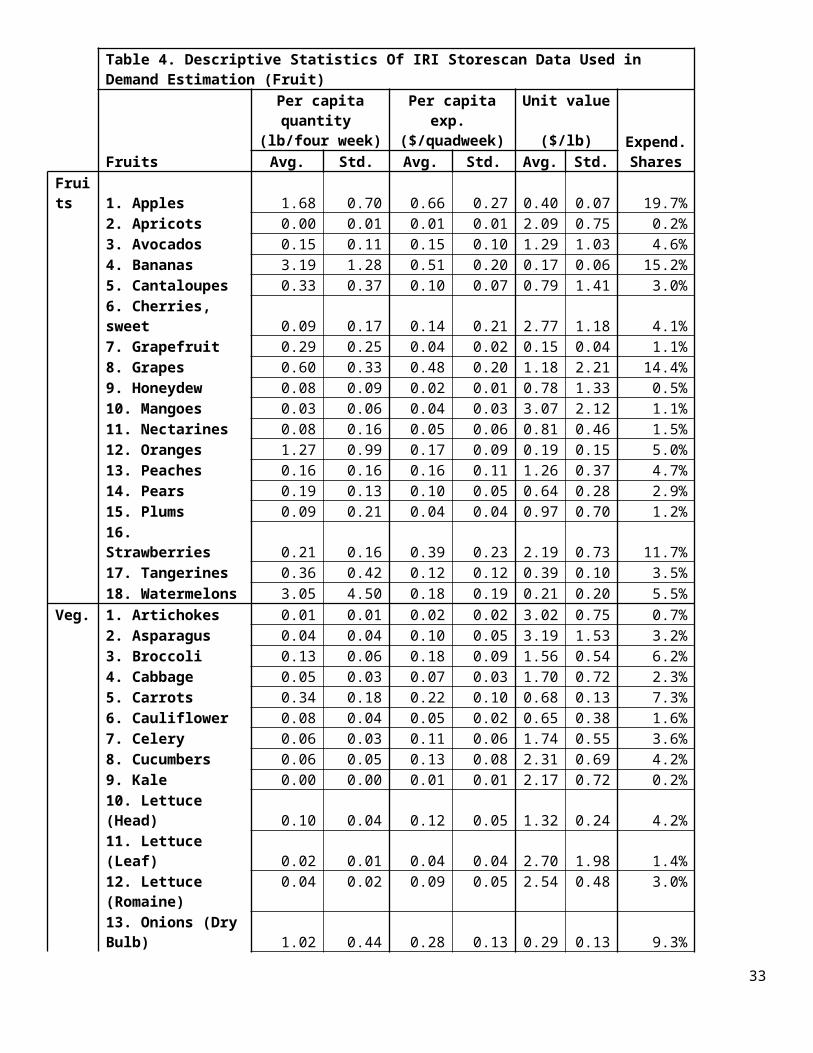
Fruit and vegetable items in InfoScan are recorded with or without per-unit weight information. Items without the weight information are called random weight items. To impute volume sales for a random weight item, we divided its dollar sales by the price of a similar nonrandom weight item from the same market and time period. This assumes random weight items have the same price as their nonrandom weight counterparts. Although imperfect, this seems to be the only feasible method for including random weight produce scanner data into a demand analysis. Summary statistics on the data used in our demand estimation is provided in Table (5).

<< Table 4 - Summary Statistics of Goods Used in Our Demand Estimation >>

To reduce the unit value bias (Deaton, 1988), we created a Fisher Ideal price index for each fruit and vegetable category. The Fisher Ideal price index is a superlative index that approximates the true cost of

11

living index for a class of expenditure function (Diewert, 1976). This allows us to account for within-category product substitution without explicitly estimating a product-level demand model for each fruit and vegetable category (Zhen, et al., 2011). We constructed the Fisher Ideal price index for category j in market m and quadweek t

(20) pmjt=√∑ pmkt qk 0

∑ pk 0qk 0

∑ pmkt qkmt

∑ pk 0qkmt,

where pmkt and qmkt are the price and per capita sales volume of product k in market m and quadweekt ,

respectively, andpk 0 and qk 0 are the base price and per capita volume of product k set at their sample means. Within each category, we defined product at the brand (name brand, no brand, private label), organic (organic, nonorganic), and type (canned, fresh, frozen) level. This yields a maximum of 18 unique products within a category. The actual number of products vary across categories because not all fruits and vegetables are available as canned or frozen type.

Demand Estimates

Tables 5 and 6 (excluded from this draft due to space limitations) provides estimates of the parameters used in the QUAIDS model. The large size of the IRI storescan panel dataset makes nearly every parameter significant in terms of being different from zero.

<< Table 5 – Parameter Estimation Results Fruit >>7

<< Table 6 – Parameter Estimation Results Veg >>8

Tables 7 and 8 provide estimates of the income elasticities and the own- and cross-price elasticities of our demand model. In these tables, the diagonal terms (highlighted in green) are the own-price elasticities of demand and are all of the expected sign (negative) for normal goods. Income elasticities are all positive, indicating these are normal goods. Cross-price elasticities are both negative, indicating goods are substitutes, and positive, indicating goods are complements (and indicated by the red cells).

<< Table 7 – Demand Elasticities for Fruits >>

<< Table 8 – Demand Elasticities for Vegetables >>

The second parts to Tables 7 and 8 provide the t-statistics for the elasticity estimates. Owing to the large panel nature of the dataset, nearly every term is significantly different from zero. While there is no a priori theoretical reason why fruits or vegetables would necessarily be substitutes (as opposed to having no effect), the finding that they are, in many cases, statistically significant complements has implications for our analysis regarding the value of exemptions and exclusions. If all fruits and vegetables were substitutes, a FSMA rule which raised the cost (and price) of other goods would

7 Owing to the large number of parameters and space constraints, Table 5 is omitted from the paper. 8 Owing to the large number of parameters and space constraints, Table 6 is omitted from the paper.

12

necessarily benefit rival commodity producers. On the other hand, if fruits and vegetables are both complements and substitutes for each other, then one can define no clear relationship a priori.

IV. Estimates

Cost Pass Through of FSMA Regulation Costs

To calculate the pass through of cost to consumer from the cost shift, we first use the EDM to calculate the effects on the variables dlP, dlQ , dlW , and dlF from the cost shift embed in the β-term in (7), With these values, we use Equations (14) and (15) to calculate the percentage of costs pass through of FSMA costs to consumers. These values are given for fruits and vegetables in Tables (9) and (10).

<< Table 9 - Shifts to Equil. Price (P,W) and Quant. (Q, X), CPT and Welfare Effects (Fruit) >>

<< Table 10 - Shifts to Equil. Price (P,W) and Quant. (Q, X), CPT and Welfare Effects (Vegetables) >>

The estimated cost pass through (CPT) varies across commodities. For fruits, if farm costs of production rise 10 percent, farm prices rise 5.68 percent while consumer prices rise 2.47 percent. For vegetables, if farm costs of production rise 10 percent, farm prices rise 6.76 percent while consumer prices rise 25.02 percent. With one good – celery – CPT was negative for both consumers and producers, an anomaly that likely occurred because celery is a complement with other goods in the demand system. As the price of these other goods rose, the demand for celery fell, an effect that overwhelmed the counteracting force of the price increase. Separately, for one good – artichokes – the quantity sold rose suggesting that artichokes were a strong substitute for similar goods whose costs also rose.

Producer Welfare Effects

Equation (13), along with the market-equilibrium shifts, are used to calculate the producer welfare effect, which is presented in Tables (9) and (10). Fruit and vegetable farmer welfare is simulated to fall by 1.11 and 0.96 percent and on average. For avocados, oranges, pears and squash, the welfare loss exceeds 2 percent of sales.

Value of Exemptions

Equation (16) is used to calculate the value of being exempt commodity producer when all other producers face cost increase. If goods are primarily substitutes, then this value is positive. If goods are primarily complements, the value is negative. Table (11) and (12) provide these estimates which are modest.

<< Table 11 - Value of Exemptions (Fruit) >>

<< Table 12 - Value of Exemptions (Vegetables) >>

For fruits, the average value of being an exempt commodity producer when other producer face cost increase is 0.09 percent. For vegetables, the value is –0.03, a value which we attribute to the measured complementarity of the commodities.

13

Value of Comprehensive Enactment

Equation (17) provides an estimate of the value of comprehensively enacting FSMA. If all producers simultaneously adopt FSMA regulations, thereby increasing costs, the price increases of rival producers potentially raises their demand and offsets a portion of their welfare loss. While some commodities experience reduced welfare, on average both fruit and vegetable producers in aggregate have welfare improvements owing to comprehensive enactment. For Fruit Producers, the VCE is 0.09 percent of total sales. For vegetable producers, the VCE is 0.36 percent.

<< Table 13 - Value of Comprehensive Enactment (Fruit) >>

<< Table 14 - Value of Comprehensive Enactment (Vegetables) >>

V. Conclusions

As the Food Safety Modernization Act and other laws are enacted, a key concerns is the size and distribution of regulatory costs on producers. In the case of food safety, producers may not witness a change in their individual commodity demand or other underlying cost that will allow them to recover the costs of compliance, even when the public health benefits of the regulation are tangible and large. At the same time, as our results show, the incidence of the costs of compliance is typically split between consumers and producers. We show that in addition to the cost of compliance varying across commodity, the extent of cost pass through varies as well. Consequently, the value of an exemption from a regulation varies across commodities as well.

A key issue in regulations and other areas of public economics is the extent to substitution across goods can exacerbate the harm of compliance costs to specific producer groups when producers of substitute goods are not regulated. We show that comprehensive enactment of a regulation does offset a portion of the producer welfare loss of the regulation relative to the unilateral enactment of that regulation. However, even for similar goods of fruits and vegetables, these benefits may be small if some goods are poor substitutes or complements.

14

VI. Appendix

Appendix 1 - Derivation of Equations (1’) to (5’) from (1) to (6)

Equations (1) through (6) are:

(1) QND=QN

D (PN , AN ),

(2) Pn=cn (W n , PMI ),

(3) X nD=(∂cn (W n ,PMI )/∂W n )Qn=gn (W n ,PMI )Qn,

(4) X nS=Xn

S (W n× (1−CS )n ),

(5) MI nD=(∂cn (W n, PMI )/∂ PMI )Qn=hn (W n ,PMI )Qn, and

(6) MI S=MI S (PMI )

In each case, take the total derivative and then rearrange terms to organize the equations in terms of elasticities (η, ε, σ) and budget shares (ω) and log changes in variables (noting that ∂ X /X=dlX , ∂ P/P=dlP, and so on.)

(A1.1) dQ=∑k=1

N ∂Q nD

∂Pkd Pn+

∂QnD

∂ AN

dlQ=∑k=1

N ∂QnD

∂ Pk

Pn

QnD dl Pn+

∂QnD

∂ A N

AN

QnD

dlQ=∑k=1

N

ηnkdl Pn+αN

dlQ−∑k=1

N

ηnkdl Pn=αN

(A1.2) d Pn=∂cn∂W n

dW n+∂cn

∂PMIdPMI

dl Pn=∂cn∂W n

W n

PndlW n+

∂cn∂ PMI

PMIPn

dlPMI

dl Pn=XnW n

Qn PndlW n+

MI nPMIQnPn

dlPMI

15

dl Pn=sndlW n+(1−sn)dlPMI

dl PN−sndlW n−(1−sn )dlPMI=0

(A1.3) d Xn=∂ gn∂W n

dW n+∂gn

∂ PMIdPMI+d Qn

dl Xn=∂ gn∂W n

W n

XndlW n+

∂gn

∂ PMIPMIX n

dlPMI+Qn

XndlQn

dl Xn=γ ndlW n+∂ gn∂ PMI

PMIXn

dlPMI+dlQ

dl Xn=sn γndlW n+(1−sn)γndlPMI+dlQ

dl Xn−γ ndlW n−γmidlPMI−dlQ=0

(A1.4) d Xn=∂ Xn

S

∂W ndW n+

∂ XnS

∂ Bnd Bn

d lXn=∂ Xn

S

∂W n

W n

XndlW n+

∂ XnS

∂Bn

Bn

Xndl Bn

d lXn=εndlW n+βn

dl Xn−εndlW n=εnβ l

(A1.5) d MI nD=

∂hn∂W n

dW n+∂hn

∂PMIdPMI+dQn

dl Xn=∂ gn∂W n

W n

XndlW n+

∂gn

∂ PMIPMIX n

dlPMI+Qn

XndlQn

dl MI n=snηn¿ dlW n+(1−sn)ηn

¿ dlPMI+dlQ

γndlW n+γmidlPMI+dlQ−dlMI n=0

(A1.6) d MI= ∂MI S

∂PMId PMI

dl MI= ∂MI S

∂ PMIPMIMI

dl PMI

dl MI=εMI dl PMI

16

( εMI )−1dl MI−dlPMI=0

If the supply of marketing inputs is perfectly elastic then εMI equals ∞ and ( εMI )−1 equals 0. Substituting

this equality into equation (6’).

(A1.6’) dlPMI=0

This solution for equation (Al.6’) can then be substituted in into (1’) to (5’) yielding the simplified equations:

(1’) dlQN−ηN dl PN=αN

(2’) dl PN−sN dlW N=0

(3’) dl X N−γN dlWN−dlQN=0

(4’) dl X N−εN dlW N=εN βN

(5’) γN dlW n+dlQN−dlMI N=0

Appendix 2 - Solving for γN and γMI as a function of sN and σ N ,MI

Note that q i is produced with two inputs xn and MI. Following equation (2) and suppressing subscripts, let the unit cost of q be c (w , pmi ) where w and pmi are the prices of the respective inputs.

(A2.1) c=c (w , pmi )

Following (Sato and Koizumi, 1973), define the elasticity of substitution as:

(A2.2) σ w ,mi=c cw ,mi

cw cmi=ccw ,mi

cw cmi=cw ,mi

cwccmi

where cw ,mi=(∂c )2/∂w∂mi , x=cx=∂c /∂w and mi=cmi=∂c /∂ pmi .

Note that the Hicksian cross-price elasticities of demand for inputs x is:

(A2.3) γmi=∂ (cw)∂ pmi

pmicw

=(∂c )2

∂w∂mipmicw

=(∂c )2

∂w∂mimicw

=cw ,mi

cwmi

Therefore,

(A2.4) σ w ,mi=cw ,mi

cwccmi

=γmic

cmimi= 1

(1−sx )γmi

17

(A2.5) γmi=(1−s x)σ w ,mi

To solve for γn, note that:

(A2.6) c=x cw+(mi ) cmi

and that:

(A2.7) ∂c=x ∂ (cw )/∂w+ (mi ) ∂ (cmi )/∂w=0

Since ∂ (cmi )∂x

=(∂c )2

∂w∂mi=∂ (cw )∂ pmi

, multiple by 1/w and simply to get:

(A2.8) γn+γmi=0

So that:

(A2.9) γn=− (1−sx) σw ,mi

18

VII. Figures and Tables

Figure 1 – The Cost of Implementing FSMA by Farm Size (Fruits)

Source: Economic Research Service, USDA as computed from USDA-NASS Ag Census Data (2012)

19

Figure 2 – The Cost of Implementing FSMA by Farm Size (Vegetables)

Source: Economic Research Service, USDA as computed from USDA-NASS Ag Census Data (2012)

20

Table 1. Estimated Average Costs to Implementing FSMA by Category Regulatory Comp. FDA’s Est. Ann. Costs Shares1 Agricultural Water $49 Mil. 13.70%2 Fertilizer/Compost of Animal Origin $9 Mil. 2.50%3 Worker Health/Hygiene Measures $81 Mil. 22.60%4 Animal Intrusion Measures $38 Mil. 10.60%5 Sanitary Standards (Equip., Tools, Build. $59 Mil. 16.50%6 Recordkeeping and Other Costs $122 Mil. 34.10% Total (Excluding Sprouts Rule) $358 Mil.  

Source: FDA Regulatory Impact Assessment of Food Safety Modernization Act Produce Rule (2015)

21

Table 2 – Estimated FSMA Cost Shifts by Commodity

FruitsCost Shift Vegetables

Cost Shift

1. Apples 2.57% 1. Artichokes 0.38%2. Apricots 2.25% 2. Asparagus 2.64%3. Avocados 4.05% 3. Broccoli 0.46%4. Bananas 4.47% 4. Cabbage 1.68%5. Cantaloupes 1.60% 5. Carrots 0.99%6. Cherries, sweet 2.92% 6. Cauliflower 0.46%7. Grapefruit 1.78% 7. Celery 0.42%8. Grapes 2.14% 8. Cucumbers 2.22%9. Honeydew 0.72% 9. Kale 0.87%10. Mangoes 6.08% 10. Lettuce (Head) 0.34%11. Nectarines 1.28% 11. Lettuce (Leaf) 0.42%12. Oranges 2.23% 12. Lettuce (Romaine) 0.31%13. Peaches 2.99% 13. Onions (Dry Bulb) 1.75%14. Pears 4.89% 14. Onions (Green) 1.25%15. Plums 2.40% 15. Peppers (Bell) 1.47%16. Strawberries 1.64% 16. Peppers (Chile) 2.83%17. Tangerines 1.41% 17. Snap Beans 3.17%18. Watermelons 2.91% 18. Spinach 0.87% 19. Squash 2.90% 20. Sweet Corn 3.17% 21. Tomatoes 1.14%Average (Expend. Weighted) 2.79% Average (Expend. Weighted) 1.52%Max 6.08% Max 3.17%Min 0.72% Min 0.31%

Source: Economic Research Service, USDA as computed from USDA-NASS Ag Census Data (2012)

22

Table 3 - Costs Shares, Elast. of Substitution, Elast. of Demand and Elast. of Supply

Cost Share (s) Elast. of Subs (σ) Dem Elast. (η) Supply Elast. (ε)Fruit 1. Apples 80.98% 0.000 -0.908 0.905 2. Apricots 32.34% 0.000 -1.209 0.800 3. Avocados 33.00% 0.000 -1.050 0.050 4. Bananas 33.00% 0.000 -0.959 2.000 5. Cantaloupes 20.46% 0.000 -1.044 0.121 6. Cherries 8.78% 0.000 -1.754 0.290 7. Grapefruit 79.44% 0.000 -1.247 0.800 8. Grapes 38.78% 0.000 -1.024 0.200 9. Honeydew 19.89% 0.000 -0.951 0.205 10. Mangoes 33.00% 0.000 -1.120 2.000 11. Nectarines 34.43% 0.000 -1.312 0.800 12. Oranges 78.94% 0.000 -1.046 0.200 13. Peaches 31.28% 0.000 -0.982 0.800 14. Pears 46.87% 0.000 -1.020 0.290 15. Plums 28.60% 0.000 -1.033 0.800 16. Strawberries 36.22% 0.000 -1.223 0.830 17. Tangerines 78.94% 0.000 -1.609 0.200 18. Watermelons 57.94% 0.000 -1.140 0.321Veg. 1. Artichokes 16.60% 0.540 -1.308 0.418 2. Asparagus 38.24% 0.540 -0.962 0.418 3. Broccoli 24.13% 0.540 -1.019 0.120 4. Cabbage 10.15% 0.540 -1.026 0.655 5. Carrots 38.89% 0.540 -1.020 0.199 6. Cauliflower 63.94% 0.540 -1.033 0.218 7. Celery 10.68% 0.540 -0.861 0.097 8. Cucumbers 9.93% 0.540 -1.031 0.327 9. Kale 18.00% 0.540 -0.464 0.650 10. Lettuce (Head) 15.97% 0.540 -0.787 0.320 11. Lettuce (Leaf) 10.60% 0.540 -1.012 1.190 12. Lettuce (Rom.) 11.26% 0.540 -0.957 0.615 13. Onions (Bulb) 53.33% 0.540 -0.798 0.194 14. Onions (Green) 18.00% 0.540 -1.004 0.097 15. Peppers (Bell) 14.33% 0.540 -0.980 0.290 16. Peppers (Chile) 14.33% 0.540 -1.191 0.290 17. Snap Beans 49.80% 0.540 -0.914 0.471 18. Spinach 18.00% 0.540 -1.012 0.335 19. Squash 12.16% 0.540 -1.005 0.120 20. Sweet Corn 20.46% 0.540 -0.846 0.477 21. Tomatoes 29.01% 0.540 -0.967 0.290

23

Table 4. Descriptive Statistics Of IRI Storescan Data Used in Demand Estimation (Fruit)

Per capita quantity

(lb/four week)Per capita exp. ($/quadweek)

Unit value ($/lb) Expend.

SharesFruits Avg. Std. Avg. Std. Avg. Std.Fruits 1. Apples 1.68 0.70 0.66 0.27 0.40 0.07 19.7% 2. Apricots 0.00 0.01 0.01 0.01 2.09 0.75 0.2% 3. Avocados 0.15 0.11 0.15 0.10 1.29 1.03 4.6% 4. Bananas 3.19 1.28 0.51 0.20 0.17 0.06 15.2% 5. Cantaloupes 0.33 0.37 0.10 0.07 0.79 1.41 3.0% 6. Cherries, sweet 0.09 0.17 0.14 0.21 2.77 1.18 4.1% 7. Grapefruit 0.29 0.25 0.04 0.02 0.15 0.04 1.1% 8. Grapes 0.60 0.33 0.48 0.20 1.18 2.21 14.4% 9. Honeydew 0.08 0.09 0.02 0.01 0.78 1.33 0.5% 10. Mangoes 0.03 0.06 0.04 0.03 3.07 2.12 1.1% 11. Nectarines 0.08 0.16 0.05 0.06 0.81 0.46 1.5% 12. Oranges 1.27 0.99 0.17 0.09 0.19 0.15 5.0% 13. Peaches 0.16 0.16 0.16 0.11 1.26 0.37 4.7% 14. Pears 0.19 0.13 0.10 0.05 0.64 0.28 2.9% 15. Plums 0.09 0.21 0.04 0.04 0.97 0.70 1.2% 16. Strawberries 0.21 0.16 0.39 0.23 2.19 0.73 11.7% 17. Tangerines 0.36 0.42 0.12 0.12 0.39 0.10 3.5% 18. Watermelons 3.05 4.50 0.18 0.19 0.21 0.20 5.5%Veg. 1. Artichokes 0.01 0.01 0.02 0.02 3.02 0.75 0.7% 2. Asparagus 0.04 0.04 0.10 0.05 3.19 1.53 3.2% 3. Broccoli 0.13 0.06 0.18 0.09 1.56 0.54 6.2% 4. Cabbage 0.05 0.03 0.07 0.03 1.70 0.72 2.3% 5. Carrots 0.34 0.18 0.22 0.10 0.68 0.13 7.3% 6. Cauliflower 0.08 0.04 0.05 0.02 0.65 0.38 1.6% 7. Celery 0.06 0.03 0.11 0.06 1.74 0.55 3.6% 8. Cucumbers 0.06 0.05 0.13 0.08 2.31 0.69 4.2% 9. Kale 0.00 0.00 0.01 0.01 2.17 0.72 0.2% 10. Lettuce (Head) 0.10 0.04 0.12 0.05 1.32 0.24 4.2% 11. Lettuce (Leaf) 0.02 0.01 0.04 0.04 2.70 1.98 1.4% 12. Lettuce (Romaine) 0.04 0.02 0.09 0.05 2.54 0.48 3.0% 13. Onions (Dry Bulb) 1.02 0.44 0.28 0.13 0.29 0.13 9.3% 14. Onions (Green) 0.01 0.01 0.04 0.02 7.81 4.02 1.3% 15. Peppers (Bell) 0.09 0.06 0.22 0.12 2.81 1.01 7.5% 16. Peppers (Chile) 0.03 0.23 0.02 0.02 2.97 1.12 0.8% 17. Snap Beans 0.15 0.09 0.17 0.09 1.20 0.26 5.6% 18. Spinach 0.02 0.01 0.05 0.03 2.37 0.47 1.7% 19. Squash 0.36 1.10 0.12 0.09 2.55 1.73 3.9% 20. Sweet Corn 0.19 0.11 0.23 0.11 1.25 0.26 7.8% 21. Tomatoes 0.46 0.23 0.72 0.31 1.67 0.40 24.2%

24

Table 7 - Price Elasticities of Demand for Fruits

Commodity Income Apples

Apricots

Avoca

does

Bananas

Cantaloupe

Cherries

Grapefru

it

Grapes

Honeydew

Mangoes

Nectar

ines

Oranges

Peaches

PearsPlums

Straw

berry

Tangerin

es

Wate

rmelon

Apples 0.877 -0.91 0.54 -0.15 -0.10 0.09 0.06 -0.15 -0.02 -0.01 -0.23 0.30 -0.11 0.20 -0.02 0.11 -0.04 0.13 0.02Apricots 0.460 0.00 -1.21 0.00 0.00 0.00 0.00 0.00 0.00 0.00 0.00 -0.01 -0.01 0.00 0.01 0.00 0.00 0.02 0.01Avocadoes 1.192 -0.01 0.06 -1.05 0.02 0.03 0.05 0.05 -0.01 -0.08 -0.06 0.23 0.02 0.00 0.02 0.02 -0.01 -0.03 -0.01Bananas 1.041 -0.05 -0.08 0.07 -0.96 0.08 -0.01 0.07 -0.03 0.07 0.01 -0.03 0.00 -0.01 -0.01 0.01 0.06 -0.02 -0.08Cantaloupe 0.732 0.01 -0.02 0.01 0.01 -1.04 0.00 0.00 0.00 0.03 -0.01 -0.18 0.01 0.03 0.02 -0.06 0.01 -0.09 -0.01Cherries 1.307 0.01 0.05 0.02 0.00 0.01 -1.75 -0.02 0.01 -0.02 0.20 0.13 -0.01 -0.03 -0.02 -0.02 0.01 0.13 -0.01Grapefruit 0.870 -0.01 -0.04 0.01 0.00 0.00 -0.03 -1.25 0.00 0.08 0.02 -0.02 0.00 0.01 0.01 -0.01 0.01 0.02 0.00Grapes 1.068 0.02 0.22 -0.05 -0.02 0.04 0.11 0.10 -1.02 0.03 0.01 0.02 0.01 -0.01 0.02 0.00 0.01 -0.03 0.00Honeydew 0.957 0.00 0.02 -0.01 0.00 0.01 -0.01 0.03 0.00 -0.95 -0.01 0.02 0.00 -0.01 0.01 0.02 0.00 -0.03 0.00Mangoes 1.214 -0.01 0.05 -0.01 0.00 0.00 0.13 0.02 0.00 -0.02 -1.12 0.15 -0.01 0.03 -0.02 -0.01 0.00 -0.04 0.01Nectarines 0.995 0.01 -0.04 0.04 0.00 -0.05 0.07 -0.01 0.00 0.03 0.12 -1.31 0.01 -0.04 0.00 -0.03 0.00 -0.11 0.05Oranges 1.011 -0.02 -0.57 0.02 0.00 0.03 -0.07 0.02 0.00 -0.02 -0.07 0.08 -1.05 0.00 -0.04 0.03 0.07 0.02 0.00Peaches 0.693 0.03 -0.05 -0.02 -0.02 0.05 -0.11 0.03 -0.02 -0.07 0.10 -0.20 -0.02 -0.98 0.05 -0.05 0.01 -0.13 0.06Pears 0.728 -0.01 0.16 0.00 -0.01 0.03 -0.07 0.01 -0.01 0.05 -0.08 0.00 -0.03 0.04 -1.02 -0.02 0.03 0.04 0.03Plums 1.097 0.01 0.00 0.00 0.00 -0.02 -0.02 0.00 0.00 0.03 -0.01 -0.03 0.01 -0.01 0.00 -1.03 0.00 -0.05 0.01Strawberry 1.042 0.00 -0.36 -0.04 0.04 0.07 0.07 0.17 0.01 0.04 -0.03 -0.06 0.15 0.08 0.15 0.03 -1.22 0.15 -0.12Tangerines 1.573 0.04 0.39 -0.01 0.01 -0.06 0.25 0.06 0.01 -0.13 -0.10 -0.33 0.02 -0.04 0.06 -0.13 0.05 -1.61 0.04Watermelon 1.127 0.01 0.40 -0.01 -0.01 0.00 -0.02 0.01 0.00 -0.01 0.03 0.25 0.01 0.06 0.05 0.03 -0.04 0.02 -1.14Green highlights the own price elasticitiesm, red highlight cross price elasticities indicated that goods are complements.

25

Table 7 (continued)- Standard Errors of Income and Price Elasticities for Fruits

Commodity Income Apples

Apricots

Avoca

does

Bananas

Cantal

oupe

Cherries

Grapefru

it

Grapes

Honeydew

Mangoes

Nectar

ines

Oranges

Peaches

PearsPlums

Straw

berry

Tange

rines

Wate

rmelon

Apples 1508.6 -957.61 25.22 -66.12 -124.97 54.51 49.87 -47.14 73.98 4.66 -54.44 63.61 -58.63 91.02 -31.29 61.02 -7.60 63.30 53.27Apricots 50.5 28.69 -236.98 14.15 -8.55 -6.20 10.31 -4.81 46.42 9.17 18.72 -11.14 -79.43 -7.05 28.91 2.38 -37.18 35.38 90.88Avocadoes 1100.3 -107.21 8.37 -1843.65 85.80 29.70 37.33 36.70 -117.79 -76.05 -71.47 119.04 32.83 -34.29 -1.98 17.80 -33.36 -10.30 -14.51Bananas 1904.6 -184.79 -19.21 121.85 -1949.29 37.34 10.78 21.83 -96.70 29.68 21.42 -11.45 -1.39 -58.95 -76.67 14.28 83.72 19.25 -75.35Cantaloupe 568.8 73.14 -8.84 70.93 88.60 -2048.04 16.37 6.12 51.29 37.70 5.05 -104.83 35.59 71.94 68.89 -59.43 49.78 -61.55 -2.03Cherries 239.2 18.71 7.00 32.96 -4.63 -0.55 -450.85 -34.38 39.91 -20.96 172.69 55.77 -28.04 -38.70 -50.10 -21.32 15.12 70.80 -8.65Grapefruit 386.2 -44.93 -5.46 51.75 36.48 -0.37 -28.13 -686.15 107.30 75.68 37.23 -15.07 9.96 18.01 11.22 -7.03 81.99 25.74 10.23Grapes 1711.3 -44.18 24.88 -72.58 -97.11 -18.71 53.71 68.26 -3042.29 10.53 32.73 4.08 3.21 -72.41 -48.61 5.74 20.94 22.18 12.75Honeydew 299.8 -0.18 8.05 -69.72 32.65 30.81 -17.02 74.11 24.32 -1301.05 -23.17 23.82 -11.89 -41.86 38.32 50.86 13.14 -40.63 -8.43Mangoes 571.8 -74.16 15.73 -72.30 6.64 -16.32 173.71 30.40 11.98 -26.74 -1633.57 131.07 -42.35 58.66 -106.35 -14.36 -12.21 -41.72 35.57Nectarines 198.6 53.67 -12.39 127.75 -8.46 -112.22 59.01 -16.52 10.16 23.57 133.09 -641.40 27.38 -65.44 -1.06 -25.33 -11.29 -73.34 122.33Oranges 655.9 -72.35 -83.30 49.57 3.20 15.23 -21.53 5.27 16.75 -13.18 -36.20 27.27 -1080.11 -21.15 -69.25 19.67 123.75 19.56 11.99Peaches 402.1 105.32 -8.41 -4.34 -12.88 75.99 -28.41 23.41 -17.29 -37.01 71.90 -62.34 -5.09 -761.40 78.72 -25.21 44.80 -38.78 91.38Pears 638.6 -9.77 27.54 34.24 -18.23 72.13 -35.12 15.24 40.38 44.52 -87.23 5.02 -51.31 75.63 -1446.16 -2.51 115.59 47.76 100.80Plums 392.1 39.09 0.20 21.70 9.00 -73.37 -18.76 -10.88 3.35 49.55 -12.81 -26.21 16.82 -34.92 -14.52 -1365.03 15.30 -58.81 25.32Strawberry 1023.5 -37.73 -42.42 -18.61 83.63 22.79 23.95 71.59 30.23 9.41 -4.19 -12.59 125.15 22.33 89.39 17.71 -956.64 56.55 -82.83Tangerines 399.0 29.53 32.55 -19.05 -9.42 -84.73 69.93 18.11 -20.54 -46.11 -45.96 -77.19 7.11 -55.52 27.78 -63.69 41.44 -288.69 29.97Watermelon 590.5 13.49 86.71 -10.86 -82.79 -23.11 -5.81 -1.11 3.24 -13.18 38.11 119.17 5.26 68.20 74.25 24.34 -91.60 38.51 -1151.78Shaded cells are not significant at the 5% level

26

Table 8 - Income and Price Elasticities of Demand for Vegetables

Income Artich

okes

Asparag

us

Brocco

li

Cabbage

Carrots

Caulifl

ower

CeleryCucu

mbers

KaleLe

ttuce (H

ead)

Lettuce

(Lea

f)

Lettuce

(Romain

e)

Onions (Dry

Bulb)

Onions (Green

)

Peppers (B

ell)

Peppers (C

hile)

Snap Bean

s

Spinac

h

Squash

Sweet

Corn

Tomato

es

Artichoke 0.679 -1.31 0.02 -0.01 0.00 -0.01 -0.05 0.00 0.01 0.35 -0.05 0.00 0.01 0.01 -0.02 0.00 0.06 0.01 0.07 -0.01 0.02 0.00Asparagus 1.043 0.09 -0.96 0.00 0.02 0.02 0.00 0.00 0.00 0.15 -0.01 0.03 -0.03 -0.03 0.03 0.00 0.02 -0.02 -0.03 -0.04 -0.02 0.01Broccoli 0.930 -0.08 -0.01 -1.02 0.00 0.08 0.03 0.04 -0.02 0.54 0.03 0.01 0.04 -0.03 0.02 0.00 0.00 -0.04 -0.03 -0.02 -0.01 0.00Cabbage 0.922 -0.01 0.01 0.00 -1.03 -0.01 -0.01 -0.01 -0.01 -0.03 0.00 0.02 -0.01 0.00 0.01 -0.01 0.02 0.06 -0.08 0.00 0.03 -0.01Carrots 0.932 -0.07 0.05 0.09 -0.03 -1.02 -0.12 0.06 -0.06 -0.32 -0.09 0.08 -0.08 -0.06 -0.01 -0.05 -0.04 0.13 -0.02 -0.02 0.10 -0.01Caulifl. 1.023 -0.12 0.00 0.01 0.00 -0.02 -1.03 -0.03 -0.02 0.21 -0.04 0.02 0.04 0.00 -0.03 0.00 0.03 0.05 0.05 0.00 0.01 0.00Celery 0.960 0.00 0.00 0.02 -0.01 0.03 -0.06 -0.86 -0.02 -0.60 0.04 0.04 -0.04 -0.03 0.01 -0.03 0.00 -0.04 -0.15 -0.01 0.02 0.01Cucumber 1.223 0.08 0.00 0.00 0.00 -0.02 -0.03 -0.02 -1.03 -0.17 -0.03 -0.01 0.00 0.01 -0.03 -0.01 0.00 0.04 -0.01 0.01 0.00 0.01Kale 1.647 0.11 0.01 0.02 0.00 -0.01 0.02 -0.03 -0.01 -0.46 -0.01 0.01 -0.02 -0.01 -0.02 0.00 -0.04 0.00 0.10 -0.01 0.00 0.00Lettuce (Head) 1.161 -0.35 -0.01 0.03 0.01 -0.04 -0.11 0.06 -0.03 -0.30 -0.79 0.04 0.03 -0.05 -0.06 0.00 0.01 0.01 -0.05 0.01 -0.01 0.01Lettuce (Leaf) 0.700 0.01 0.01 0.00 0.01 0.01 0.01 0.01 -0.01 0.03 0.01 -1.01 0.04 0.00 0.00 -0.01 0.02 0.00 0.01 0.01 -0.01 -0.01Lettuce (Rom.) 1.171 0.05 -0.03 0.02 0.00 -0.03 0.07 -0.02 0.00 -0.28 0.02 0.10 -0.96 -0.01 0.02 0.01 -0.03 -0.01 0.07 0.00 -0.03 0.00Onions (Bulb) 1.146 0.27 -0.07 -0.02 0.03 -0.06 0.01 -0.06 0.01 -0.37 -0.11 0.05 -0.04 -0.80 0.00 -0.01 0.12 -0.03 -0.04 0.01 -0.05 0.00Onions (Green) 1.031 -0.03 0.01 0.00 0.01 0.00 -0.02 0.00 -0.01 -0.17 -0.02 0.00 0.01 0.00 -1.00 -0.01 0.01 0.02 0.01 0.00 0.01 0.00Peppers (Bell) 1.219 0.08 0.02 0.02 -0.02 -0.03 0.03 -0.04 -0.03 -0.18 0.00 -0.01 0.02 0.00 -0.05 -0.98 -0.21 0.00 0.10 -0.02 -0.02 0.01Peppers (Chile) 1.193 0.06 0.01 0.00 0.01 0.00 0.01 0.00 0.00 -0.15 0.00 0.01 -0.01 0.01 0.01 -0.02 -1.19 0.02 -0.03 0.00 0.00 0.00Snap Beans 0.713 0.09 -0.06 -0.05 0.13 0.09 0.16 -0.08 0.03 -0.03 -0.02 -0.01 -0.05 -0.04 0.08 -0.03 0.17 -0.91 -0.15 -0.05 0.10 -0.03Spinach 1.111 0.20 -0.01 -0.01 -0.06 0.00 0.05 -0.07 -0.01 0.89 -0.02 0.02 0.04 -0.01 0.02 0.02 -0.08 -0.04 -1.01 -0.03 0.01 0.01Squash 1.171 -0.02 -0.04 -0.01 0.01 0.00 0.00 0.00 0.00 -0.27 0.00 0.04 0.00 0.01 0.01 -0.01 0.01 -0.02 -0.05 -1.00 0.00 0.01Sweet Corn 0.696 0.32 -0.07 -0.04 0.09 0.10 0.00 0.02 -0.04 -0.20 -0.06 -0.05 -0.12 -0.08 0.04 -0.06 0.00 0.14 0.02 -0.03 -0.85 -0.03Tomatoes 0.987 -0.05 0.09 0.00 -0.08 -0.01 0.00 0.05 0.01 -0.29 -0.01 -0.08 -0.03 -0.04 -0.04 -0.02 -0.08 -0.07 0.12 0.04 -0.02 -0.97

27

Table 8 -(continued)- Standard Errors of Income and Price Elasticities for Vegetables

Income Artich

okes

Asparag

us

Brocco

li

Cabbage

Carrots

Caulifl

ower

CeleryCucu

mbers

KaleLe

ttuce (H

ead)

Lettuce

(Leaf)

Lettuce

(Romain

e)

Onions (Dry

Bulb)

Onions (Green

)

Peppers (B

ell)

Peppers (C

hile)

Snap Bean

s

Spinach

Squash

Sweet

Corn

Tomato

es

Artichoke 176.1 -397.2 63.6 -27.9 -5.8 -10.7 -54.6 -0.5 43.7 79.8 -99.7 3.9 17.4 75.9 -25.8 25.2 56.4 17.9 59.9 -17.1 87.1 -11.4Asparagus 984.0 54.6 -1457.5 -21.4 23.4 52.5 -4.3 5.0 5.1 69.5 -26.3 14.6 -73.3 -86.4 72.6 29.2 22.6 -64.7 -33.7 -93.0 -82.7 74.1Broccoli 1713.6 -32.7 -6.8 -1949.4 3.7 165.7 39.8 72.8 -0.4 100.4 80.6 -4.7 68.5 -44.4 30.7 52.2 7.8 -93.6 -18.1 -26.4 -65.2 5.5Cabbage 722.8 -7.7 30.6 4.2 -942.7 -17.0 -6.4 -8.0 -2.2 -2.9 14.8 9.5 -2.5 25.4 20.6 -15.7 17.1 81.4 -88.7 13.8 58.0 -46.6Carrots 1268.6 -13.7 64.2 165.4 -17.6 -706.8 -58.7 52.4 -56.7 -27.7 -60.9 28.4 -42.7 -91.3 -5.0 -45.2 -9.0 86.2 -4.9 -3.9 132.0 -12.9Caulifl. 830.3 -57.6 -3.3 33.6 -9.0 -62.0 -1315.1 -65.1 -49.1 55.0 -101.5 10.7 74.5 10.7 -58.9 38.1 31.7 105.6 60.6 1.4 1.4 2.7Celery 1067.6 -4.0 11.6 68.5 -9.4 50.5 -62.6 -1046.8 -37.9 -104.2 97.1 20.3 -39.3 -84.0 16.4 -62.4 6.8 -86.2 -111.5 -4.5 22.6 44.0Cucumber 1923.7 32.5 -18.3 -43.7 -20.5 -86.1 -61.7 -62.8 -2762.1 -43.7 -70.0 -26.3 -1.5 30.4 -81.7 -78.2 -1.3 42.1 -15.3 20.1 -65.3 22.4Kale 236.1 78.4 62.4 91.7 -6.8 -32.9 52.4 -109.6 -48.4 -119.0 -48.2 6.3 -41.9 -70.3 -72.8 -36.2 -62.6 -2.9 140.7 -126.5 -26.7 -37.1Lettuce (Head) 1628.5 -105.3 -39.7 52.0 4.0 -75.9 -106.9 84.2 -63.7 -45.4 -988.2 12.6 32.8 -200.0 -106.6 -5.9 3.3 -16.3 -34.7 19.9 -71.2 -13.4Lettuce (Leaf) 195.6 4.0 22.0 4.3 12.9 34.9 15.6 27.0 -6.6 9.5 25.7 -423.7 90.4 20.6 3.1 -7.0 17.5 -4.8 18.2 32.9 -15.3 -21.2Lettuce (Rom.) 1461.1 12.6 -85.3 48.5 -10.9 -53.7 70.4 -49.7 3.3 -40.2 32.5 78.8 -768.1 -49.1 18.2 29.1 -25.5 -40.4 47.3 -10.8 -113.3 -30.4Onions (Bulb) 1664.9 62.1 -98.6 -88.9 6.5 -116.1 -0.5 -102.0 46.1 -60.2 -186.7 3.4 -44.7 -1254.5 -7.2 -0.8 48.9 -84.7 -38.4 22.7 -130.0 -50.9Onions (Green) 1022.0 -29.0 74.7 22.8 16.5 -10.3 -59.1 12.9 -64.2 -69.5 -95.5 -3.2 24.3 4.4 -2984.4 -64.2 22.8 76.5 33.8 20.3 43.0 -32.5Peppers (Bell) 2165.5 11.5 7.2 -10.3 -38.9 -80.9 19.4 -96.0 -78.1 -29.2 -13.1 -28.1 23.7 -15.0 -81.6 -2086.5 -123.0 -60.3 94.2 -49.1 -120.5 -30.0Peppers (Chile) 342.8 53.3 18.9 -1.1 13.2 -15.0 28.7 1.9 -1.1 -61.4 1.8 13.6 -26.0 46.0 19.0 -120.0 -827.9 69.2 -50.3 9.9 1.4 -22.9Snap Beans 660.8 18.1 -43.8 -71.2 90.3 98.9 115.7 -72.8 82.8 3.4 11.4 -5.1 -19.8 -37.1 94.8 0.2 82.5 -523.2 -54.6 -56.0 124.8 -76.1Spinach 696.2 57.9 -38.1 -28.5 -94.7 -9.3 58.8 -115.7 -9.9 142.4 -33.2 12.2 48.3 -36.4 32.0 102.8 -49.9 -64.2 -409.2 -105.6 12.8 75.9Squash 687.4 -31.6 -104.4 -65.3 -5.3 -35.0 -10.2 -28.2 26.8 -115.8 17.4 18.8 -10.1 17.8 7.5 -38.4 11.0 -100.4 -107.3 -1236.3 -28.2 30.1Sweet Corn 790.8 88.1 -53.3 -32.4 70.3 158.1 20.9 45.2 4.5 -16.4 -26.7 -15.2 -74.2 -75.5 71.5 -36.0 12.8 125.5 33.9 14.2 -718.0 -18.3Tomatoes 2216.8 -26.6 78.7 -19.9 -52.0 -25.0 9.0 33.5 99.8 -14.9 34.2 -37.6 11.5 3.5 -21.1 62.6 -5.6 -123.8 82.4 70.0 -89.9 -1663.3Shaded cells are not significant at the 5% level

28

Commodity Exp. Shares dlQ dlP CPT - Cons. dlX dlW dlMI CPT - Farm ΔPS1. Apples 19.7% -1.10% 1.12% 43.66% -1.10% 1.39% -1.10% 53.9% -1.18%2. Apricots 0.2% -0.58% 0.50% 22.21% -0.58% 1.54% -0.58% 68.7% -0.70%3. Avocadoes 4.6% -0.17% 0.22% 5.47% -0.17% 0.67% -0.17% 16.6% -3.37%4. Bananas 15.2% -1.32% 1.29% 28.89% -1.32% 3.91% -1.32% 87.5% -0.55%5. Cantaloupes 3.0% -0.15% 0.07% 4.51% -0.15% 0.35% -0.15% 22.0% -1.25%6. Cherries 4.1% -0.03% 0.25% 8.61% -0.03% 2.86% -0.03% 98.0% -0.06%7. Grapefruit 1.1% -0.78% 0.65% 36.45% -0.78% 0.82% -0.78% 45.9% -0.96%8. Grapes 14.4% -0.21% 0.43% 19.89% -0.21% 1.10% -0.21% 51.3% -1.04%9. Honeydew 0.5% -0.06% 0.09% 11.98% -0.06% 0.43% -0.06% 60.2% -0.29%10. Mangoes 1.1% -1.86% 1.76% 28.99% -1.86% 5.34% -1.86% 87.8% -0.73%11. Nectarines 1.5% -0.24% 0.34% 26.48% -0.24% 0.98% -0.24% 76.9% -0.30%12. Oranges 5.0% -0.44% 0.05% 2.06% -0.44% 0.06% -0.44% 2.6% -2.17%13. Peaches 4.7% -0.60% 0.72% 23.91% -0.60% 2.29% -0.60% 76.5% -0.70%14. Pears 2.9% -0.91% 0.87% 17.85% -0.91% 1.86% -0.91% 38.1% -3.01%15. Plums 1.2% -0.54% 0.50% 20.85% -0.54% 1.75% -0.54% 72.9% -0.65%16. Strawberries 11.7% -0.43% 0.41% 25.11% -0.43% 1.13% -0.43% 69.3% -0.50%17. Tangerines 3.5% -0.24% 0.19% 13.30% -0.24% 0.24% -0.24% 16.8% -1.17%18. Watermelons 5.5% -0.50% 0.81% 27.83% -0.50% 1.40% -0.50% 48.0% -1.51%

Average -0.67% 0.70% 24.77% -0.67% 1.68% -0.67% 56.87% -1.11%

Table 9 - Shifts to Equilibrium Price (P,W) and Quantities (Q, X) and Cost Pass Through (Fruit)

29

Commodity Exp. Share dlQ dlP CPT - Cons. dlX dlW dlMI CPT - Farm ΔPS/Exp1. Artichokes 0.72% 0.01% 0.03% 8.75% -0.07% 0.20% 0.10% 52.74% -0.18%2. Asparagus 3.24% -0.37% 0.38% 14.46% -0.70% 1.00% -0.04% 37.82% -1.64%3. Broccoli 6.15% -0.01% 0.02% 4.48% -0.05% 0.09% 0.03% 18.58% -0.38%4. Cabbage 2.28% -0.06% 0.09% 5.59% -0.50% 0.92% 0.39% 55.05% -0.75%5. Carrots 7.28% -0.05% 0.11% 11.12% -0.14% 0.28% 0.05% 28.60% -0.71%6. Cauliflower 1.58% -0.04% 0.09% 19.68% -0.07% 0.14% -0.01% 30.78% -0.32%7. Celery 3.63% -0.09% -0.01% -1.94% -0.05% -0.08% -0.12% -18.20% -0.50%8. Cucumbers 4.22% -0.07% 0.08% 3.64% -0.47% 0.81% 0.32% 36.62% -1.40%9. Kale 0.24% -0.03% 0.09% 10.10% -0.25% 0.49% 0.18% 56.09% -0.38%10. Lettuce (Head) 4.15% -0.07% 0.01% 2.14% -0.09% 0.05% -0.05% 13.39% -0.30%11. Lettuce (Leaf) 1.36% -0.02% 0.03% 7.20% -0.16% 0.29% 0.12% 67.95% -0.14%12. Lettuce (Rom.) 2.98% -0.06% 0.01% 4.49% -0.12% 0.13% 0.00% 39.88% -0.19%13. Onions (Bulb) 9.31% -0.21% 0.16% 9.37% -0.28% 0.31% -0.13% 17.57% -1.44%14. Onions (Gr.) 1.28% -0.03% 0.03% 2.52% -0.10% 0.18% 0.05% 14.01% -1.08%15. Peppers (Bell) 7.53% -0.10% 0.06% 4.27% -0.30% 0.44% 0.10% 29.79% -1.03%16. Peppers (Ch.) 0.81% -0.15% 0.13% 4.60% -0.57% 0.91% 0.27% 32.10% -1.91%17. Snap Beans 5.58% -0.55% 0.65% 20.54% -0.90% 1.31% -0.19% 41.24% -1.85%18. Spinach 1.75% -0.02% 0.06% 7.37% -0.17% 0.35% 0.14% 40.92% -0.51%19. Squash 3.88% -0.10% 0.05% 1.79% -0.30% 0.43% 0.10% 14.72% -2.47%20. Sweet Corn 7.78% -0.21% 0.30% 9.48% -0.84% 1.47% 0.43% 46.36% -1.70%21. Tomatoes 24.23% -0.14% 0.08% 7.17% -0.25% 0.28% -0.04% 24.70% -0.86%

Average -0.13% 0.12% 6.76% -0.30% 0.44% 0.04% 25.02% -0.96%

Table 10 - Shifts to Equilibrium Price (P,W) and Quantities (Q, X) and Cost Pass Through (Vegetables)

30

Commodity Exp. Shares dlQ dlP dlX dlW dlMI ΔPS/Exp1. Apples 19.7% -1.05% 1.17% -1.05% 1.45% -1.05% -1.12%2. Apricots 0.2% -0.59% 0.50% -0.59% 1.53% -0.59% -0.71%3. Avocadoes 4.6% -0.18% 0.17% -0.18% 0.52% -0.18% -3.52%4. Bananas 15.2% -1.24% 1.30% -1.24% 3.95% -1.24% -0.52%5. Cantaloupes 3.0% -0.12% 0.12% -0.12% 0.59% -0.12% -1.02%6. Cherries 4.1% -0.29% 0.17% -0.29% 1.94% -0.29% -0.97%7. Grapefruit 1.1% -0.79% 0.64% -0.79% 0.80% -0.79% -0.97%8. Grapes 14.4% -0.29% 0.28% -0.29% 0.73% -0.29% -1.41%9. Honeydew 0.5% -0.07% 0.07% -0.07% 0.38% -0.07% -0.34%10. Mangoes 1.1% -1.93% 1.75% -1.93% 5.31% -1.93% -0.77%11. Nectarines 1.5% -0.36% 0.29% -0.36% 0.83% -0.36% -0.44%12. Oranges 5.0% -0.36% 0.35% -0.36% 0.44% -0.36% -1.78%13. Peaches 4.7% -0.67% 0.69% -0.67% 2.20% -0.67% -0.79%14. Pears 2.9% -0.90% 0.89% -0.90% 1.90% -0.90% -2.97%15. Plums 1.2% -0.52% 0.51% -0.52% 1.78% -0.52% -0.62%16. Strawberries 11.7% -0.47% 0.39% -0.47% 1.08% -0.47% -0.55%17. Tangerines 3.5% -0.24% 0.15% -0.24% 0.20% -0.24% -1.21%18. Watermelons 5.5% -0.64% 0.56% -0.64% 0.97% -0.64% -1.93%Average -0.68% 0.68% -0.68% 1.58% -0.68% -1.20%

Table 11 - The Shifts to Price (P,W), Quantities (Q, X) and Welfare Measures Associated with a Unilaterally Implementing FSMA Regs (Fruit)

31

Commodity Exp. Share dlQ dlP dlX dlW dlMI ΔPS/Exp1. Artichokes 0.72% -0.03% 0.02% -0.10% 0.15% 0.03% -0.23%2. Asparagus 3.24% -0.37% 0.38% -0.70% 1.00% -0.03% -1.64%3. Broccoli 6.15% -0.02% 0.02% -0.05% 0.07% 0.01% -0.39%4. Cabbage 2.28% -0.09% 0.09% -0.52% 0.89% 0.34% -0.79%5. Carrots 7.28% -0.08% 0.08% -0.16% 0.22% -0.01% -0.77%6. Cauliflower 1.58% -0.06% 0.06% -0.08% 0.09% -0.04% -0.37%7. Celery 3.63% -0.01% 0.01% -0.04% 0.06% 0.02% -0.36%8. Cucumbers 4.22% -0.08% 0.08% -0.47% 0.80% 0.31% -1.41%9. Kale 0.24% -0.04% 0.09% -0.25% 0.48% 0.18% -0.38%10. Lettuce (Head) 4.15% -0.02% 0.02% -0.07% 0.12% 0.04% -0.22%11. Lettuce (Leaf) 1.36% -0.03% 0.03% -0.17% 0.28% 0.11% -0.14%12. Lettuce (Rom.) 2.98% -0.02% 0.02% -0.09% 0.16% 0.06% -0.15%13. Onions (Bulb) 9.31% -0.17% 0.21% -0.27% 0.40% -0.07% -1.36%14. Onions (Gr.) 1.28% -0.03% 0.03% -0.11% 0.17% 0.04% -1.08%15. Peppers (Bell) 7.53% -0.07% 0.07% -0.29% 0.48% 0.15% -0.99%16. Peppers (Ch.) 0.81% -0.15% 0.13% -0.57% 0.90% 0.26% -1.92%17. Snap Beans 5.58% -0.57% 0.64% -0.91% 1.28% -0.22% -1.88%18. Spinach 1.75% -0.05% 0.05% -0.19% 0.30% 0.08% -0.56%19. Squash 3.88% -0.06% 0.06% -0.29% 0.49% 0.17% -2.40%20. Sweet Corn 7.78% -0.24% 0.29% -0.86% 1.43% 0.37% -1.74%21. Tomatoes 24.23% -0.10% 0.10% -0.23% 0.35% 0.04% -0.79%

Average -0.11% 0.13% -0.30% 0.46% 0.07% -0.93%

Table 12 - The Shifts to Price (P,W), Quantities (Q, X) and Welfare from Unilaterally Implementing FSMA Regs (Vegetables)

32

Commodity Exp. Shares dlQ dlP dlX dlW dlMI ΔPS/Exp1. Apples 19.7% -0.05% -0.05% -0.05% -0.06% -0.05% -0.06%2. Apricots 0.2% 0.01% 0.00% 0.01% 0.01% 0.01% 0.01%3. Avocadoes 4.6% 0.01% 0.05% 0.01% 0.15% 0.01% 0.15%4. Bananas 15.2% -0.08% -0.01% -0.08% -0.04% -0.08% -0.04%5. Cantaloupes 3.0% -0.03% -0.05% -0.03% -0.23% -0.03% -0.23%6. Cherries 4.1% 0.27% 0.08% 0.27% 0.91% 0.27% 0.92%7. Grapefruit 1.1% 0.01% 0.01% 0.01% 0.01% 0.01% 0.01%8. Grapes 14.4% 0.07% 0.14% 0.07% 0.37% 0.07% 0.37%9. Honeydew 0.5% 0.01% 0.01% 0.01% 0.06% 0.01% 0.06%10. Mangoes 1.1% 0.07% 0.01% 0.07% 0.03% 0.07% 0.03%11. Nectarines 1.5% 0.12% 0.05% 0.12% 0.15% 0.12% 0.15%12. Oranges 5.0% -0.08% -0.30% -0.08% -0.38% -0.08% -0.38%13. Peaches 4.7% 0.07% 0.03% 0.07% 0.08% 0.07% 0.08%14. Pears 2.9% -0.01% -0.02% -0.01% -0.04% -0.01% -0.04%15. Plums 1.2% -0.02% -0.01% -0.02% -0.03% -0.02% -0.03%16. Strawberries 11.7% 0.04% 0.02% 0.04% 0.05% 0.04% 0.05%17. Tangerines 3.5% 0.01% 0.03% 0.01% 0.04% 0.01% 0.04%18. Watermelons 5.5% 0.14% 0.25% 0.14% 0.43% 0.14% 0.43%Average 0.01% 0.02% 0.01% 0.09% 0.01% 0.09%

Table 13 - The Shifts to Price (P,W), Quantities (Q, X) and Welfare Measures Associated with a Exemption by Commodity (Fruit)

33

Commodity Exp. Share dlQ dlP dlX dlW dlMI ΔPS/Exp1. Artichokes 0.72% 0.05% 0.01% 0.02% 0.05% 0.07% 0.05%2. Asparagus 3.24% 0.00% 0.00% 0.00% 0.00% 0.00% 0.00%3. Broccoli 6.15% 0.01% 0.00% 0.00% 0.01% 0.01% 0.01%4. Cabbage 2.28% 0.04% 0.00% 0.02% 0.03% 0.05% 0.03%5. Carrots 7.28% 0.04% 0.03% 0.01% 0.07% 0.06% 0.07%6. Cauliflower 1.58% 0.02% 0.03% 0.01% 0.05% 0.03% 0.05%7. Celery 3.63% -0.08% -0.01% -0.01% -0.14% -0.15% -0.14%8. Cucumbers 4.22% 0.01% 0.00% 0.00% 0.01% 0.02% 0.01%9. Kale 0.24% 0.00% 0.00% 0.00% 0.00% 0.00% 0.00%10. Lettuce (Head) 4.15% -0.06% -0.01% -0.02% -0.08% -0.09% -0.08%11. Lettuce (Leaf) 1.36% 0.01% 0.00% 0.00% 0.00% 0.01% 0.00%12. Lettuce (Rom.) 2.98% -0.04% 0.00% -0.02% -0.04% -0.06% -0.04%13. Onions (Bulb) 9.31% -0.04% -0.05% -0.02% -0.09% -0.06% -0.09%14. Onions (Gr.) 1.28% 0.00% 0.00% 0.00% 0.01% 0.01% 0.01%15. Peppers (Bell) 7.53% -0.03% -0.01% -0.01% -0.04% -0.05% -0.04%16. Peppers (Ch.) 0.81% 0.00% 0.00% 0.00% 0.01% 0.01% 0.01%17. Snap Beans 5.58% 0.02% 0.02% 0.01% 0.03% 0.03% 0.03%18. Spinach 1.75% 0.04% 0.01% 0.02% 0.05% 0.06% 0.05%19. Squash 3.88% -0.04% -0.01% -0.01% -0.07% -0.07% -0.07%20. Sweet Corn 7.78% 0.04% 0.01% 0.02% 0.04% 0.05% 0.04%21. Tomatoes 24.23% -0.05% -0.02% -0.02% -0.07% -0.07% -0.07%

Average -0.02% -0.01% -0.01% -0.03% -0.03% -0.03%

Table 14 -- The Shifts to Price (P,W), Quantities (Q, X) and Welfare Measures Associated with an Exemption by Commodity (Vegetables)

34

VIII. References

Banks, J., R. Blundell, and A. Lewbel. 1997. "Quadratic Engel Curves and Consumer Demand." The Review of Economics and Statistics 79(4):527-539.

California Division of Industrial Relations. 2014. “Cal/OSHA–Title 8 regulations–Section 3457, Field Sanitation.” http://www.dir.ca.gov/title8/3457.html. Accessed January 11, 2014.

Deaton, A. 1988. "Quality, Quantity, and Spatial Variation of Price." The American Economic Review 78(3):418-430.

Diewert, W.E. 1976. "Exact and superlative index numbers." Journal of Econometrics 4(2):115-145.Johnson, R. 2011. "The FDA Food Safety Modernization Act (P.L. 111-353)." Congressional Research

Service Report.Johnson, R. 2014. "The U.S. Food Safety System: A Primer." Congressional Research Service Report

RS22600.Okrent, A.M., and J.M. Alston. 2012. "The Effects of Farm Commodity and Retail Food Policies on

Obesity and Economic Welfare in the United States." American Journal of Agricultural Economics 94(3):611-646.

Sato, R., and T. Koizumi. 1973. "On the elasticities of substitution and complementarity." Oxford Economic Papers 25(1):44-56.

Stewart, H. 2006. How Low has the Farm Share of Retail Food Prices Really Fallen? Washington, DC: Economic Research Service

Wohlgenant, M.K. 1989. "Demand for Farm Output in a Complete System of Demand Functions." American Journal of Agricultural Economics 71(2):241-252.

Zhen, C., M.K. Wohlgenant, S. Karns, and P. Kaufman. 2011. "Habit Formation and Demand for Sugar-Sweetened Beverages." American Journal of Agricultural Economics 93(1):175-193.

35