Embed Size (px)
Citation preview
RHEINISCHE FRIEDRICH-WILHELMS-UNIVERSITÄT BONN
Faculty of Agriculture
&
WAGENINGEN UNIVERSITY & RESEARCH
Agricultural Economics and Rural Policy Group
MASTERTHESIS
As part of the Master programme’s
Agricultural and Food Economics
&
Management, Economics and Consumer Studies
Submitted in partial fulfilment of the requirements for the degree of
,,Master of Science”
Volatility spillovers between meat markets, feed markets and energy markets
submitted by:
Björn Meier
880216-554-100
submitted on: 30.05.2017
first examiner: Prof. Dr. T. Heckelei
second examiner: Dr. C. Gardebroek
I
Table of contents
List of figures ................................................................................................ III
List of tables .................................................................................................. IV
List of acronyms ............................................................................................. V
1 Introduction .............................................................................................. 1
2 Literature review ...................................................................................... 3
Futures market ........................................................................................................ 3 2.1
Meat market ............................................................................................................ 5 2.2
Feed market ............................................................................................................ 7 2.3
2.3.1 Grain market .......................................................................................................... 7
2.3.2 Soybean market ..................................................................................................... 8
Energy market ........................................................................................................ 9 2.4
Volatility in the futures market ............................................................................ 10 2.5
Volatility spillovers within the agricultural market ............................................. 12 2.6
Volatility spillovers between agricultural and the energy market ........................ 13 2.7
Summary .............................................................................................................. 14 2.8
3 Methodology ............................................................................................ 16
Stationarity ........................................................................................................... 17 3.1
Vector autoregressive models .............................................................................. 18 3.2
Forecast error variance ......................................................................................... 23 3.3
Structural analysis ................................................................................................ 24 3.4
3.4.1 Generalized impulse response function ............................................................... 24
3.4.2 Generalized forecast error variance decomposition ............................................ 25
Volatility spillover indices ................................................................................... 26 3.5
4 Data and model estimation .................................................................... 29
Data ..................................................................................................................... 29 4.1
Annualized range volatilities, closing prices and trade volumes ......................... 30 4.2
II
Stationarity tests ................................................................................................... 35 4.3
Model specification and estimation ...................................................................... 36 4.4
5 Empirical results ..................................................................................... 39
Total volatility spillover index ............................................................................. 39 5.1
Directional and net volatility spillover indices .................................................... 40 5.2
5.2.1 Livestock .............................................................................................................. 40
5.2.2 Feed crops ............................................................................................................ 42
5.2.3 Energy .................................................................................................................. 43
Pairwise volatility spillover indices ..................................................................... 44 5.3
5.3.1 Livestock-Livestock ............................................................................................ 44
5.3.2 Livestock–Feed .................................................................................................... 45
5.3.3 Energy–Livestock ................................................................................................ 47
5.3.4 Feed-Feed ............................................................................................................ 48
5.3.5 Feed–Energy ........................................................................................................ 49
5.3.6 Summary .............................................................................................................. 50
Discussion ............................................................................................................ 50 5.4
6 Concluding remarks ............................................................................... 55
References .................................................................................................... 57
Appendix ...................................................................................................... 64
Appendix 1: Eigenvalues VAR (5) .................................................................................... 64
Appendix 2: Results of sensitivity analysis ....................................................................... 65
Appendix 3: Pairwise net volatility relationships .............................................................. 67
Declaration ................................................................................................... 68
III
List of figures
Figure 1: Global meat production .............................................................................................. 5
Figure 2: Methodology overview ............................................................................................. 16
Figure 3: Livestock futures data ............................................................................................... 31
Figure 4: Feed crop futures data ............................................................................................... 33
Figure 5: Crude oil futures data ................................................................................................ 34
Figure 6: Total trading volume ................................................................................................. 35
Figure 7: Total volatility spillover index .................................................................................. 39
Figure 8: Livestock directional and net spillover indices ........................................................ 41
Figure 9: Feed directional and net spillover indices ................................................................ 43
Figure 10: Crude oil directional and net spillover indices ....................................................... 44
Figure 11: Livestock pairwise volatility spillovers .................................................................. 45
Figure 12: Livestock-feed pairwise volatility spillovers .......................................................... 46
Figure 13: Energy-livestock pairwise volatility spillovers ...................................................... 48
Figure 14: Feed-feed pairwise volatility spillovers .................................................................. 49
Figure 15: Feed-energy pairwise volatility spillovers .............................................................. 49

IV
List of tables
Table 1: Results ADF test ........................................................................................................ 36
Table 2: Results SIC (full sample) ........................................................................................... 37
V
List of acronyms
ADF Augmented Dickey-Fuller
AIC Akaike information criterion
CBOT Chicago Board of Trade
CME Chicago Mercantile Exchange
DF Dickey-Fuller
FEV Forecast error variance
FEVD Forecast error variance decomposition
GARCH Generalized autoregressive conditional heteroskedasticity
GFEVD Generalized forecast error variance decomposition
GI Generalized impulse response function
HQIC Hannan-Quinn information criterion
MGARCH Multivariate generalized autoregressive conditional heteroskedasticity
MMT Million metric tons
MSE Mean squared error
NYMEX New York Mercantile Exchange
OLS Ordinary least squares
SIC Schwarz information criterion
SRW Soft Red Winter
VAR Vector autoregressive
VMA Vector moving average
1
1 Introduction
The commodity price crisis in 2008, besides surging commodity prices also caused an un-
precedented interest of the scientific community in price volatility and volatility linkages in
commodity markets (Minot 2014). Price volatility is a concept that estimates the extent of
price variability over time. This variability of a commodity price at a certain point in time can
be spilled over into other commodity markets. News in one market can have implications for
other markets and vice versa, which results in volatility relationships between markets that
share information. Traders in commodity exchanges use these relationships between markets
to continuously adjust their future expectation of a price to new market intelligence. Thus they
can forward price variations in one market to another market based on their perception of
market interconnectivity. The focus in research regarding commodity price volatility relation-
ships in recent times has been on linkages between the energy and agricultural sector. An in-
creasing demand for agricultural raw materials originated in the energy sector after policies
have been introduced in several countries that stimulated the production of crude oil substi-
tutes, based on agricultural inputs. This linkage of the agricultural market to the energy mar-
ket provides many opportunities for traders to speculate or to hedge their market price risk
since a price movement in one market can be answered by a corresponding price movements
in the other market.
Another substantial shift in the demand for agricultural staples occurred due to developments
in the livestock sector. The global per capita consumption of meat-based proteins almost dou-
bled throughout the last four decades, while the overall share of proteins in the human diet
remains constant. Thus, proteins originating in plants are increasingly replaced by proteins
obtained from the livestock sector. A good example for this development is to be found in
China where meat consumption per capita per day was surging from 4.2 grams in 1961 to
37.2 grams in 2011. Feed conversion ratios translate this into an increasing total calorie de-
mand since producing one livestock calorie requires several feed calories. The vast increases
in meat consumption concentrate on emerging economies such as China, Brazil or Mexico,
but also high income countries like Japan or Spain significantly increased their consumption
levels (Sans and Combris 2015). The increasing demand for meat in these nations also affects
other economies. According to FAOSTAT the USA, which is the largest global pork exporter,
experienced almost a 7000 percent increase in its pork meat exports since 1961 with Japan
and Mexico depicting the largest importers (USDA 2017a).
2
The objective of this thesis is to determine the effect that increasing meat consumption has on
the volatility relationship between livestock and crop futures prices. Furthermore, due to the
competition between the livestock and energy sector for scarce agricultural resources, which
increases the amount of information shared between the two sectors, the energy sector is also
a part of the analysis. Ultimately, the thesis will answer the following four research questions:
Did the total volatility spillovers between the meat market, feed market and energy market
increase over time?
Is the flow of volatility happening unidirectional from input into output markets?
Which commodities transmit and which commodities receive more volatility over time?
What is the influence of the energy sector on volatility spillovers?
Until recently the methodological focus in volatility related studies has been almost exclusive-
ly on GARCH-type models, which were introduced by Bollerslev (1986) as an extension to
Engle (1982). Anyway, the methodology applied in this thesis is built upon an alternative es-
timation procedure, which was introduced by Diebold and Yilmaz (2012). This approach al-
lows for an extended market network and can capture time-varying effects in the data sample.
The thesis does not figure as an attempt to compare the two methodologies or to provide any
form of statement regarding superiority of one to the other.
The thesis is divided into six distinct sections. After the introductory chapter the literature
review begins, which familiarizes the reader with the markets included in the analysis and
presents relevant results regarding volatility in the futures market and volatility spillovers
between the commodity markets. In chapter three the methodology applied in the analysis is
elaborated, introducing first a stationarity test for time series data and afterwards going into
vector autoregressive models and their capabilities to analyze relationships between variables
in a multivariate time series setup. The indices to measure the volatility spillovers are estab-
lished at the end of chapter three. The subsequent chapter four contains the model specifica-
tion and estimation plus an extended description of the data. In chapter five the empirical re-
sults of the volatility spillover indices are presented successively and discussed at the end of
the chapter. The thesis ends with a brief summary and concluding remarks in chapter six.
3
2 Literature review
This chapter gives an overview about the most relevant aspects regarding the fundamental
developments in the agricultural sector with respect to the increasing meat consumption and
its evolving relationship to the energy sector. Furthermore, the commodity futures market
itself is introduced. Literature is used to identify the patterns that these developments caused
regarding commodity price volatility spillovers. Following this goal, the chapter first intro-
duces the relevant markets and subsequently volatility in the futures market and volatility
spillovers within the agricultural markets as well as between the agricultural and energy mar-
kets are discussed. Price developments of the individual commodities are presented with the
data in chapter four.
Futures market 2.1
The first futures market was established 1848 in Chicago, namely the Chicago Board of Trade
(CBOT). The purpose of this new institution was to provide a location for all grain suppliers
and customers to conduct their business. In 2007 the CBOT merged with its greatest competi-
tor, the Chicago Mercantile Exchange (CME), into the CME Group to form the world’s larg-
est market for derivatives. In 2008 the New York Mercantile Exchange (NYMEX) joined the
CME Group. Within the CME Group, agricultural futures like soybeans or grains are traded in
the CBOT division, while livestock and energy futures are traded in the CME and in the NY-
MEX division respectively (Garner 2010).
The commodity futures contracts traded in the exchange between the traders are expiring
agreements to exchange a commodity with a predefined quantity and quality at a specific time
and a specific location. The delivery date of the contract links the commodity price today to
its future expectation. The contracts are standardized, thus all traders in one market are deal-
ing with identical contracts. The only variable for futures contracts is the price, which specu-
lators constantly try to predict accurately to earn a profit. The futures market knows two basic
position, the short position and the long position. If a trader takes a short position on the fu-
tures market he is taking the position of selling the commodity, while a long position would
be equivalent to buying the commodity. However, only a small minority of all contracts lead
to a physical exchange of the commodity. The rest of the contracts is offset before the expir-
ing date by traders taking the opposite position of their initial contract. The price variations
are restricted for certain commodities to prevent a speculative excess to cause large move-
ments of commodity prices (Hull 2012). In the futures market the price of a commodity is not
4
only influenced by fundamental demand and supply factors but can also incorporate other
futures market specific factors, like option expiration dates or margin calls (Garner 2010).
Three distinct types of traders are operating inside the futures market. Hedgers use futures
contracts to reduce the risk from potential price movements in their specific market. The arbi-
trageurs are seeking risk-free profits in the markets, which is keeping the futures markets in
balance and bound to spot market prices. The speculators, which depict the largest group, are
using their market intelligence to bet on prices to go up or down in the future (Garner 2010).
The speculators are competing in collecting and interpreting all kinds of market-related in-
formation, resulting in a competitive discovering of prices (Natarajan et al. 2014). Lehecka et
al. (2014) provide some recent empirical evidence for this statement with respect to the corn
market. The authors use per minute return volatility and trading volume from July 2009 until
May 2012 to show that the publication of the USDA corn market report has significant posi-
tive effects on both these variables. Thus, a futures price contains the collective expectation
for the future price of the commodity. The advances in information technology and global
networking continuously improve the processing of incoming news, which allows domestic
markets to quickly adjust to news from world markets. Today, this competitive price discov-
ery process is one of the key economic functions of the futures market (Natarajan et al. 2014).
The liquidity of a market measures the ability of the market to transform assets into cash
money, i.e. how quickly a contract can be sold. To form a liquid market there must be enough
traders with opposing interests, i.e. buyers and sellers. Suitable proxies for market liquidity
are the open interest and the contract trade volume of a specific market. Throughout this the-
sis the focus lies on the contract trade volume as a liquidity proxy since it has widely been
recognized as the appropriate measure for information flows (Floros and Salvador 2016).
The structure of the futures market remained rather constant from its beginnings in the mid-
19th
century until the beginning of the 21st century. But since the new millennium started im-
portant changes happened. The trading changed from an open outcry and telephone based
platform into an electronic system, which caused a significant market access expansion of the
commodity futures markets. The markets saw many new participants entering, for example
pension funds, which increased market liquidity. This development has been named the finan-
cialization of commodity markets (Irwin and Sanders 2012). The financialization of the fu-
tures market was followed by the commodity price crisis in 2008, which saw vast increases in
commodity prices. However, Irwin et al. (2009) cannot find statistical evidence for a causal
connection between the two events. The authors conclude that economic fundamentals
5
changed, i.e. changes in supply and demand, and subsequently caused the boom and bust in
the futures market. The largest increases of the total trading volume happened after 2006,
which coincides with the time when trading in the pit had been mostly replaced by electronic
ordering (Irwin and Sander 2012).
Meat market 2.2
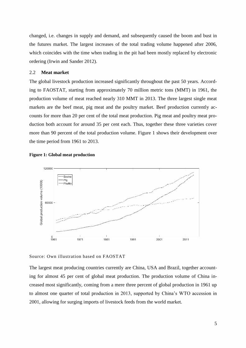
The global livestock production increased significantly throughout the past 50 years. Accord-
ing to FAOSTAT, starting from approximately 70 million metric tons (MMT) in 1961, the
production volume of meat reached nearly 310 MMT in 2013. The three largest single meat
markets are the beef meat, pig meat and the poultry market. Beef production currently ac-
counts for more than 20 per cent of the total meat production. Pig meat and poultry meat pro-
duction both account for around 35 per cent each. Thus, together these three varieties cover
more than 90 percent of the total production volume. Figure 1 shows their development over
the time period from 1961 to 2013.
Figure 1: Global meat production
Source: Own illustration based on FAOSTAT
The largest meat producing countries currently are China, USA and Brazil, together account-
ing for almost 45 per cent of global meat production. The production volume of China in-
creased most significantly, coming from a mere three percent of global production in 1961 up
to almost one quarter of total production in 2013, supported by China’s WTO accession in
2001, allowing for surging imports of livestock feeds from the world market.
6
The first futures contract for a living animal was introduced by the CME in 1964 for live cat-
tle, followed by lean hog futures in 1966. (Clark 2014). Today the livestock futures traded
within the CME Group are live cattle futures, feeder cattle futures and lean hog futures. The
live cattle futures contract has a volume of 18 metric tons and results in physical delivery of
the product if not offset by the trader beforehand. The contracts are always listed for the up-
coming nine month with expiration dates in February, April, June, August, October and De-
cember. Feeder cattle futures have a volume of 23 metric tons and do not end in physically
delivery of the product, but are financially settled. The contracts are listed for the upcoming
eight month with expiration dates in January, March, April, May, August, September, October
and November (CME 2017a). Feeder cattle futures are dealing with cattle that have reached
around 300 kg and subsequently are sold to feedlots. In the feedlots, feeder cattle are fattened
up to their slaughter weight of around 550 kg and afterwards are traded as live cattle towards
the slaughterhouses (Ryan 2012). Lean hog futures contain a volume of 18 metric tons and are
also finically settled after their expiration (CME 2017a). The trading volumes of livestock
futures have experienced among the most drastic increases of all agricultural futures markets
since the beginning of the new millennium (Irwin and Sanders 2012).
The lack of a futures market for poultry at the CME Group is due to the level of vertical inte-
gration of the chicken industry in the USA. Giant producers integrated all steps of the produc-
tion process and possess long-term contracts with large customers, which ends in a very nar-
row price range for this commodity. Furthermore, the production cycles of poultry are rela-
tively short if compared to other livestock production systems and thus supply can react to
changes in demand rather quickly. These reasons add up to low demand for hedging or specu-
lation in the poultry futures market and attempts to introduce a vital futures market repeatedly
ended up with trading volumes going down to zero (DePillis 2014).
The meat market exercises a fundamental relationship with feed crop markets and changes in
these input market can have long-term effects on price levels or price variations in the meat
markets and vice versa. The meat markets themselves are related to each other since a lot of
market information is shared between them as they compete for similar natural resources. The
meat market has a direct and an indirect fundamental relationship with energy markets. Di-
rectly it uses energy as a production input. The indirect relationship is via biofuels. Biofuel
production uses agricultural products and thus figures as an additional competitor for limited
natural resources (Gardebroek and Hernandez 2013).
7
Feed market 2.3
The focus of this sub-chapter is on feed components used in intensive indoor livestock pro-
duction systems for beef and pig meat. The most important feed crops for livestock produc-
tion in this context are grains and oilseeds that have high natural protein content, especially
soybeans. First, the grain markets are introduced, concentrating on corn and wheat. After-
wards, the soybean market is discussed, figuring as the representative for oilseed markets.
2.3.1 Grain market
Grains depict the key staple food for human consumption and a major input for livestock diets
throughout the globe. The direct human consumption of grains is decreasing with increasing
wealth, whilst indirect consumption of grains, for example as an input to livestock production,
is increasing (Gilbert and Morgan 2010). Wheat occupies the largest share of global crop land
and it can easily be stored or transported. Most of the wheat is consumed by humans, although
it is also very suitable for animal feeding (Sariannidis 2011). The plantation of winter wheat
in the USA, a major producer of wheat, happens mostly around October, while the harvesting
takes place mostly in June and July. Despite wheat, corn is another major grain. In the USA,
the largest producer of corn, planting of the crop usually takes place in late April and early
June, while the harvest comes in between October and November (USDA 2010). The demand
for corn in recent decades changed, as more and more of the corn production got allocated
into the livestock sector where corn is a key feed compound. Additionally, the developments
in the energy sector are fueling the demand for corn throughout the last decade (Shiferaw et
al. 2011). One externality of the increasing demand for corn in biofuel production so far has
been that wheat is becoming more relevant as a feed crop in the livestock sector (Gilbert and
Mugera 2014). The introduction of genetically modified corn varieties started in 1996 and
nowadays accounts for around 80 per cent of the corn production in the USA (USDA 2017b).
For the upcoming years, strong increases in demand for grains are expected, which needs to
be met with further intensification (Neumann et al. 2010). A third major grain is rice, which is
mostly consumed within Asia and western Africa. It is however not closely linked to other
grains with respect to production or consumption and it does not play a mentionable role in
the feed market (Gilbert and Morgan 2010).
Following FAOSTAT data, the global production volume of grains in MMT from 1961 until
2013 more than quadrupled. The main driver behind this increase used to be the intensifica-
tion of production (Neumann et al. 2010). The period of the slowest increases in the total pro-
duction volume of wheat took place between 1990 and 2007. This contributed to the mini-

8
mum grain stocks that were available in 2007, which also played a role in the subsequent fi-
nancial crisis (Wright 2011). Even though the growth rates of the corn production volume
were increasing during the last decade, its production volume is still not sufficient to provide
enough of the product to satisfy total demand (Vohra et al. 2014).
The first standardized wheat and corn futures contracts have officially been introduced to the
CBOT in 1865 for farmers to hedge their price risks (Sariannidis 2011) and since 2003 these
contracts have experienced dramatic increases in their trading volumes (Irwin and Sanders
2012). In recent times, corn has had the highest trading volumes of all agricultural commodi-
ties within the CME Group, with Chicago Soft Red Winter (SRW) wheat futures following on
third position (CME 2017b). The corn futures contract consists of 127 metric tons and results
in physical delivery in case the trader does not offset his position before the expiration date.
The CME lists five corn contracts with expiration dates in the upcoming months of March,
May, July, September and December. For wheat, the contract contains a volume of 136 metric
tons and the same conditions for contract settlement as for corn futures regarding delivery and
contract expiration dates (CME 2017c).
2.3.2 Soybean market
Soybeans are experiencing the highest increases in cultivated lands in percentage terms of all
crops since the 1970s (Hartman et al. 2011). In MMT, the production volume of soybeans
increased from roughly 27000 in 1961 up to almost 280000 in 2013, based on FAOSTAT.
The production concentrates on the USA, Brazil and Argentina, who combined are responsi-
ble for more than 80 per cent of global soybean production. Soybeans depict a vital input to
the livestock sector and China currently imports more than 60 MMT of soybeans per year to
allow for the fast increases in its meat production volumes (Song et al. 2009). Most of the
soybean production nowadays relies on genetically modified varieties, which were introduced
to the USA in 1994. Since the soybean seeds are very rich in protein and fat, their main pur-
pose is in livestock feeding and edible oil production. The increasing demand for soybeans is
likely to be met by area expansions, which is mainly taking place in South America (Hartman
et al. 2011). The plantation dates for soybeans in the USA, the largest producer of soybeans,
are mostly in May and harvesting takes place in September and October (USDA 2010).
The futures contract for soybeans at the CBOT was launched in 1936 and since then devel-
oped to the agricultural commodity with the second highest trading volume (CME 2017b).
The contract contains 136 metric tons and results in physical delivery of the commodity. The
contracts listed at the CME Group are expiring in January, March, May, July, August, Sep-
9
tember and November (CME 2017c). Despite the vast growth in livestock futures trading vol-
ume, the growth in trading volumes of soybean futures also soared since 2003. Between the
years 2000 and 2003 about 1.2 million contracts have been traded per month. This number
more than tripled over the course of the subsequent years (Irwin and Sanders 2012). The fun-
damental relationship between corn and soybeans in the US market, i.e. both are summer
crops competing for land resources, results in highly correlated futures prices between the two
commodities (Goodwin and Zhao 2011).
Energy market 2.4
The attention energy markets receive from researchers experienced a vast increase after the
food price crisis of 2008 (Irwin et al. 2009). The academic community widely agrees that bio-
fuel policies contributed to the circumstances that led to the crisis. Several countries, like the
USA, Brazil or the European Union, introduced certain biofuel policies, which substantially
stimulated the production. Between 2005 and 2014 the volume of bioethanol production in-
creased from 46 billion liters to 114 billion liters and the biodiesel production volume in-
creased from 3.7 billion liters up to around 30 billion liters over the same time. These devel-
opments are suspected to have caused increases in price variations and price levels in the agri-
cultural market (Enrisco et al. 2016).
The production of bioethanol, which is the most relevant biofuel, mostly depends on agricul-
tural feedstocks, for example corn in the USA or sugarcane in Brazil (Gardebroek and Her-
nandez 2013). Biodiesel production is mainly based on vegetable oils, such as rapeseed and
soybean oil (Chuah et al. 2017). Since biofuels depict a direct substitute for crude oil, the vast
increase in biofuel production creates an intensified linkage for the agricultural market to the
energy sector. Changes in the oil price will directly alter the demand for biofuels and subse-
quently influence the demand for certain agricultural crops that figure as feedstock for biofuel
production. The manifold linkages within the agricultural market like competition for land
resources or substitution in demand provide the possibility that a change in oil prices might
influence many other agricultural markets (Gardebroek and Hernandez 2013). Wright (2014)
argues that the introduction of biofuel policies fundamentally changed the structure of the
agricultural market by significantly lowering the amount of products available for human con-
sumption or livestock feeding.
Crude oil futures are the commodity with the highest average daily trading volume in the
CME Group and ethanol futures gained high liquidity only recently. Therefore, in this thesis
the focus will be on crude oil futures (CME 2017b). The crude oil futures contract at the
10
NYMEX has a volume of 1000 barrels and ultimately is settled by delivery. The contracts are
listed for the upcoming nine years, with consecutive contracts listed for each month in the
following five years and contracts for June and December from the sixth year onward (CME
2017d).
Volatility in the futures market 2.5
The advances in information technology ensure the distribution of information from all
around the world and the futures traders incorporate these into the commodity prices. Due to
the immediate processing and individual interpretation of new information, prices can vary in
the very short-run, which causes price volatility. The volatility of a price is describing the
extent of its variability over time, generally measured as the standard deviation of a relative
change in prices (Gilbert and Morgan 2010). Unconditional volatility is describing the historic
volatility of the time series, i.e. it is not conditioned upon information that is available today
and it treats every observation alike. Therefore, it does not depend on time. Conditional vola-
tility does depend on time. It determines volatility that is conditioned upon information that is
available today (Enders 2010). Throughout the following chapters volatility refers to the con-
cept of conditional volatility, if not explicitly mentioned differently. In fundamentally related
markets, i.e. markets that share common information, a shock to the volatility can spill over
from one commodity market into another related market. Therefore, analyzing the volatility
interdependency between different markets does provide insights on how information is flow-
ing between them (Liu and An 2011). Volatility spillovers can be separated into two distinct
categories. The own price volatility spillover describes volatility that is spilled from a past
volatility shock into the current price volatility within one market. Cross volatility spillovers
describe the relationship between the current volatility in one market and a past shock to the
volatility in another related market (Natarajan et al. 2014). Throughout the thesis the term
volatility spillover refers to the concept of cross volatility spillover.
The efficient market hypothesis, based on distinct assumptions about rational decision mak-
ing, states that a liquid market will drive the futures price of a commodity towards its funda-
mental price, with informed traders outcompeting less informed traders in the information
processing activities (Gosh et al. 2012). The efficient market hypothesis experienced lots of
criticism, for example from Akerlof and Shiller (2009), claiming that increasing market li-
quidity does not necessarily provide more stability due to the irrational behavior of many
speculators. The efficient market hypothesis is widely accepted only in its semi-strong form,
which states that current information are all included in the price of a commodity and that
11
new information about supply or demand fundamentals will be incorporated continuously
(UN 2011). Sanders et al. (2008) claim that the increasing number of speculators in the fu-
tures market might be changing the fundamental rules of the game by disrupting the conver-
gence patterns between cash and futures prices and thus creating price distortions.
Recently, increasing evidence has been gathered that the financialization of the commodity
futures markets is associated with increasing return- and range-based volatility. Floros and
Salvador (2016), including daily CBOT futures data of corn, soybean, sugar and wheat from
January 1996 until December 2014 in their analysis, conclude that increasing trade volumes
have a significant positive effect on the return volatility of the included commodities. Return
volatility measures the volatility of a relative change in prices over a fixed period of time, for
example taking the daily closing price of commodities (Gilbert and Morgan 2010). The posi-
tive effect implies that higher trade volumes are associated with higher return volatility in
futures markets. The authors claim their findings to be in line with leading theories on the
relationship between trade volume and conditional volatility in the futures market, like the
sequential information arrival hypothesis (Floros and Salvador 2016).
A positive correlation between trading volume in the futures market and weekly return volatil-
ity on the spot market has been detected for several agricultural markets by Gosh et al. (2012).
Additionally, the authors state that the changes in global supply and demand are not sufficient
to figure as the exclusive explanation for increasing prices and volatility, but that the finan-
cialization of the futures market also might play a vital role due to significant increases in
return volatility during times of high trading volumes. For the energy market Ripple and
Moosa (2009) find that increasing trade volumes have a significant and positive influence on
the range volatility of crude oil futures, estimated using daily futures data obtained from the
NYMEX division of the CME Group for the period between January 1995 and December
2005. Range volatility describes a volatility measure obtained from the difference between the
highest and the lowest price in a defined period (Martens and van Dijk 2006). The insight that
the trade volume could have a significant positive effect on conditional volatility in commodi-
ty futures markets has already been known before the recent drastic increases in trade vol-
umes. Using daily futures data, Bessembinder and Seguin (1993) already showed the positive
relationship between daily return volatility and trade volume for the time between 1982 until
1990, including data on agricultural commodities like wheat and cotton.
Although there is evidence for a positive correlation between trading volume and conditional
volatility, either return based or range based, this does not yet determine the direction of the
12
causal relationship (Gosh et al. 2012). The question whether higher price variations attract
more speculators or whether more speculators lead to higher price variations still needs to be
finally answered.
Volatility spillovers within the agricultural market 2.6
The literature regarding volatility spillovers between livestock and feed markets is scarce.
One of the few peer-reviewed studies concentrating on the transmission of return volatility
between livestock and feed markets was published by Buguk et al. (2003). The authors used
monthly average spot prices for corn, soybeans and catfishes in the USA from January 1980
until December 2000 in an exponential generalized autoregressive conditional heteroskedas-
ticity (GARCH) model for their analysis. The choice for the catfish market was based on the
assumption of unidirectional volatility spillovers, i.e. catfish markets are assumed to be too
small in order to influence corn and soybean markets. The results of the study indicate signifi-
cant spillovers of return volatility from input markets into the livestock market. Apergis and
Rezitis (2003) provide insights for the Greek agricultural market. The authors use monthly
indices for spot prices of agricultural input prices, agricultural output prices and food prices
from January 1985 until December 1999 to investigate the price volatility relationship be-
tween these categories. The results from the multivariate generalized autoregressive condi-
tional heteroskedasticity (MGARCH) model indicate that price volatility from agricultural
input markets positively effects volatility in agricultural output markets.
Gardebroek et al. (2016) use CBOT daily, weekly and monthly return volatilities to investi-
gate the relationship between major agricultural futures markets, namely corn, wheat and soy-
beans from January 1998 until October 2012 in an MGARCH framework. From the daily re-
turns the authors do not obtain significant evidence for return volatility spillovers when using
their full sample period. Only when analyzing the post 2008 sample individually, significant
return volatility spillovers were identified. The findings indicate that mainly wheat and corn
are transmitters of return volatility into others agricultural markets, which is similar to the
authors findings for weekly and monthly return volatility analysis. The authors hypothesize
that for daily trading the actions on the futures market are more likely to be financially moti-
vated and thus increase with numbers of speculators on the market, although this hypothesis is
not confirmed by their data. The significance of weekly and monthly average return volatility
spillovers indicates that these measures are not so much driven by speculators but are more
likely explained by fundamental relationships between the commodities.
13
Beckmann and Czudaj (2014) are using daily return volatility for corn and wheat futures from
the CBOT and cotton futures from the New York Board of Trade from January 2000 until
June 2012 in a GARCH model to analyze the return volatility relationship among some of the
most liquid agricultural commodity markets. The results of the authors show significant short-
run volatility spillovers between the commodity markets. Goodwin and Zhao (2011) use
weekly data on option contracts for the soybean and corn markets between May 2001 and
January 2010 for an analysis of the implied volatility in a threshold vector autoregressive
(VAR) model. The results indicate that in times of low implied volatility in both markets, im-
plied volatility is only transmitted from the corn market into the soybean market. In times of
higher implied volatility in the soybean market, the corn market receives implied volatility
from the soybean market. Additionally, the authors use average weekly return volatility of
corn and soybeans futures in an MGRACH model, which indicates that return volatility is
transmitted and received by both commodities.
Grosche and Heckelei (2014) use daily range volatilities to analyze the range volatility rela-
tionships between agricultural, energy, real estate and financial assets. The paper contains
volatility spillover indices, based on Diebold and Yilmaz (2012), showing volatility relation-
ships between the included assets. The authors include CBOT corn, soybeans and wheat fu-
tures data from June 1998 until December 2013. The results of the authors indicate that corn
is mostly a transmitter of conditional range volatility towards soybeans and wheat. The condi-
tional range volatility relationship between soybean and wheat is changing continuously.
Volatility spillovers between agricultural and the energy market 2.7
The introduction of biofuel policies in the USA, Brazil or the EU and the connections they
provided between the agricultural and the energy sector initiated an increase in the interest of
researchers in the information flow between these two sectors. However, so far publications
do not provide a unique perspective on this issue.
Serra and Zilberman (2013) provide a literature review regarding price transmission between
the energy sector and the agricultural sector, but also including several studies on the volatili-
ty relationship. The authors conclude that based on their literature review it seems like price
variations are mostly transmitted by the energy sector and received by the agricultural sector
and that this pattern intensified with the rise of the biofuel sector. However, the authors do not
specifically distinguish between the different volatility concepts.
14
Gardebroek and Hernandez (2013) use weekly average crude oil and corn spot price returns
with ethanol CBOT futures price returns from September 1997 until October 2011 in various
MGARCH model specifications to answer the question whether price volatility in the energy
sector influences the volatility in the corn market. The authors cannot find empirical evidence
for significant spillovers of conditional mean price return volatility from energy markets into
the corn market when analyzing the full sample period. They do find spillovers from the corn
market into the ethanol market for a segmented smaller sample. Trujillo-Barrera et al. (2012)
use return volatilities of corn, ethanol and crude oil futures from July 2006 until November
2011 to answer a similar research question in an MGARCH framework. The authors’ results
indicate strong return volatility spillovers from crude oil towards corn and ethanol, with spill-
overs being particularly strong towards the latter. Additionally, the authors find significant
return volatility spillovers from the corn market into the ethanol market but not vice versa.
Guan et al. (2011) use corn spot and CBOT futures return volatility with NYMEX crude oil
futures return volatility to investigate their return volatility relationship between January 1992
and June 2009 in a GARCH model. Their analysis shows that return volatility spillovers in-
creased significantly after 2005 and were transmitted from the crude oil market into the corn
cash and futures market.
Nazlioglu et al. (2013) utilize daily spot price data between January 1986 and March 2011 to
determine the return volatility of crude oil, soybeans, wheat and sugar. The authors split the
data in two parts, with the 31st of December 2005 taken as the separation date to have a pre-
crisis sample and a post-crisis sample to analyze in the GARCH model. The results of the
analysis suggest no return volatility spillovers before the crisis and significant spillovers
transmitted from crude oil into the agricultural markets after the crisis. The authors conclude
that throughout recent years the interdependency between the energy sector and the agricul-
tural sector increased substantially. Gilbert and Mugera (2014) use daily returns of crude oil,
corn, wheat and soybean futures markets from January 2000 until December 2011 in a
GARCH and MGARCH framework to identify the return volatility relationship amongst the
commodities. The authors find empirical evidence that during the 2008-2009 crisis the return
volatility of the crops partly increased due to volatility transmitted to them from the crude oil
market, even though this influence was only modest.
Summary 2.8
The changes that the agricultural sector experienced throughout the last two decades are ex-
traordinary. The agricultural futures market experienced an inflow of new market participant
15
and a subsequent surge in trading volumes, which seems to imply an increase in the condi-
tional return or range volatility measures of many commodity markets. Furthermore, the de-
velopments in the energy sector further tightened agricultural markets with a wide array of
potential implications. So far, the increase in meat consumption hardly caused any interest in
the volatility spillover implications that this might have. Anyway, the insights gained from the
literature review indicate that in the spot market livestock products receive volatility from
other markets. With respect to volatility in futures market it is important to keep in mind that
the concepts discussed in this chapter often do not allow to directly compare the results of
different studies and generalizations can often not be made due to distinct definitions of cer-
tain concepts.
16
3 Methodology
The research questions as presented in the introduction demand for a rigorous statistical anal-
ysis. At the center of this volatility analysis are VAR models, which are used to determine the
relationships between the individual range volatilities of the commodities included in the sys-
tem. VAR models were developed as an answer to the shortcomings of simultaneous equation
models and were introduced by Sims (1980) as a means of analyzing the relationships among
variables using their common history. In a VAR system, all variables are endogenous and in
its standard or reduced form every variable is written as a linear function of the lagged values
of all the variables included in the system. The structural analysis of reduced VAR models has
been suffering from the shortcoming due to the ordering effect of the Cholesky decomposition
of the error covariance matrix, which has been solved by Pesaran and Shin (1998) building on
Koop et al. (1996). The generalization of the structural analysis by these authors has been
developed into a framework for volatility spillover analysis by Diebold and Yilmaz (2012).
This framework allows for the investigation of volatility relationships and thus provides the
required insights with respect to the research questions. Figure 2 provides a brief overview of
the methodology used for the analysis.
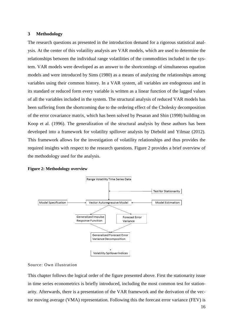
Figure 2: Methodology overview
Source: Own illustration
This chapter follows the logical order of the figure presented above. First the stationarity issue
in time series econometrics is briefly introduced, including the most common test for station-
arity. Afterwards, there is a presentation of the VAR framework and the derivation of the vec-
tor moving average (VMA) representation. Following this the forecast error variance (FEV) is
17
explained as the first element of the generalized forecast error variance decomposition
(GFEVD). The next section explains the Generalized Impulse response function (GI) as the
second element of the GFEVD. The two elements are subsequently brought together in the
sub-chapter regarding the GFEVD. The chapter ends with the introduction of the volatility
spillover indices as introduced by Diebold and Yilmaz (2012).
Stationarity 3.1
For a stochastic process to be stationary it is required that a change in time does not alter the
joint probability distribution of the process. This implies that the probability density function
for is constant over time. For most of the cases it is sufficient to use the definition of weak
stationarity, which only requires the mean, variance and covariance to be independent of time
(Verbeek 2012). A violation of the weak stationarity implies that the past realizations of a
variable cannot be used to predict future values since the distribution of the series is changing
over time. This change in the distribution over time is mostly caused by a trend or a unit root
in the data sample, where the latter can be dealt with by integrating the series. Regarding the
estimation of VAR models there is an ongoing discussion whether the variables must be sta-
tionary. Sims (1980) argues that integrating variables is taking valuable information out of the
system and that the main cause for VAR models is to investigate the relationship between the
variables based on this information. Anyway, the majority opinion in applied econometrics is
that variables included in VAR systems ought to be stationary (Enders 2010).
In the literature, a wide range of test regarding stationarity of a time series process exists. The
standard approach to test for stationarity is the Dickey-Fuller (DF) test, introduced by Dickey
and Fuller (1979). The test checks the presence of a unit root or certain trends in the data se-
quence with the of non-stationarity using a t-test with a critical value distribution specifi-
cally designed for this test. The lag length of a time series process must be determined by an
information criteria, like the Schwarz Information Criteria (SIC) (Enders 2010). The DF test
for a first order autoregressive model comes in three varieties
(1) ,
(2) ,
(3) ,
with the equations testing for a pure random walk, a random walk with drift and a random
walk with drift and a time trend, respectively. The appropriate form has to be selected due to a
visual inspection of the data (Enders 2010). A random walk due to a unit root is implied by
18
not being significantly different from zero, which leaves the value of one period equal to the
former periods’ value plus a white noise term. In that case the series would violate the condi-
tion that its second moment must be time-invariant since the variance would increase over
time. In case of a random walk with drift due to a unit root, the drift parameter depicts a de-
terministic trend in the data sequence. If the non-stationarity is due to a deterministic trend
and not due to a unit root, i.e. | | and in (22), including t in the regression makes
the sequence trend stationary. For the latter cases, also the first moment of the series is not
constant over time (Enders 2010). In case the model is of higher order, an augmented Dickey-
Fuller (ADF) test is applied. For this extension of the DF test consider the process with two
significant lags
(4) ,
rearranging this equation leads to the form used in the ADF test
(5) ( ) .
It is tested whether the term in brackets significantly differs from zero. In case it does not, the
ADF test implies that the process has a unit root and should be used in first differences. Like
the former version of the DF test also the augmented test can be extended by a trend parame-
ter, which might imply that detrending is necessary to have a stationary process (Verbeek
2012).
Vector autoregressive models 3.2
A VAR system can be represented either in a structural form or in its reduced form, with the
latter being derived from the former one. The structural form of the VAR suffers from prob-
lems like simultaneous equation biases since the current values of other variables in the sys-
tem are considered as well. To circumvent these issues and make the VAR more usable it is
transformed into its reduced or standard form (Dougherty 2011). Consider the two variables a
and b, which both have time-invariant first and second moments and thus are stationary (Lüt-
kepohl 2007). A simple structural VAR(1) model including the variables a and b would have
the form of
(6) ,
(7) ,
where the error terms and having constant and finite variance, zero covariance and
zero expectation, which leaves the error terms as white noise. The white noise describes a
19
purely random process that cannot be caught by a model. In case this assumption does not
hold for the error term there would still be information in the error term that could be extract-
ed by introducing the appropriate variable to the system. The structure contained in this
VAR(1) system allows for feedback between the individual variables and if and are
not equal to zero also the error terms indirectly effect the other equation, leaving ordinary
least squares a biased and inconsistent estimator (Enders 2010). Transforming (1) and (2) into
matrix notation gives
(8) [
] [
] [
] [
] [
] [
]
Equation (3) can be rewritten as
(9) ,
using [
] [
] [
] [
] and [
] . Multiplying
(4) with brings the VAR(1) into its standard form
(10) ,
with being the vector containing the intercepts, * being the
coefficient matrix and being the vector with the error terms (Enders
2010). Equation (5) then contains
(11) ,
(12) ,
which are the reduced forms of (1) and (2), solved for the simultaneous equation bias. There-
fore, each individual equation of a VAR model can consistently and unbiasedly be estimated
using ordinary least squares (OLS). In a VAR system, all equations are estimated simultane-
ously, not subsequently, which emphasizes its dynamic character (Enders 2010). Lütkepohl
(2007) imposes some additional requirements for the OLS estimator to be consistent, which
will be addressed later. The error terms in equations (6) and (7) depict composites of the error
terms from the structural equations and are white noise processes. Furthermore, the two error
terms are correlated, with the covariance given as
(13) (
) ( ) ,
with and
being the variances of the error terms. Correlation between the error terms
implies the possibility that a shock to one error term can cause a shock to other error term as

20
well. For the special case of the error terms would not be correlated, which
means that no contemporaneous effect exists. However, the correlation between the error
terms has no effect on the consistency and unbiasedness of the OLS estimator plus asymptoti-
cally it is efficient (Enders 2010). Since all components of the variance/ covariance matrix of
the error terms are time-invariant it can be defined as
(14) [
],
with and being the covariance between variable a and b (Enders 2010). For it is
assumed that the inverse exists, i.e. the matrix is nonsingular.
If the data generation process is investigated starting in period it has the following im-
plication
(15)
( )
( ) ,
with being a identity matrix. Continuing this process until period t gives
(16) ( )
∑
,
indicating that the vectors and joint distribution of all are being determined from the joint
distribution of the variables (Lütkepohl 2007). Assuming that the process for
started in the infinite past provides some convenient insights. It shows that if all eigenvalues
of have a modulus of less than one it is possible to build the absolute sum of the sequence
, which is equivalent to the condition
(17) ( ) with | | .
This is called the stability condition for VAR models. If the stability condition for VAR(p)
models is met, this already implies stationarity, although the reverse is not true and an unsta-
ble VAR does not necessarily have to indicate unstationary in the variables. In case the VAR
does not exhibit stability due to a unit-root, differencing the included variables often solves
the issue (Lütkepohl 2007). If the stability condition is met it is possible to determine a VAR
process beginning in the infinite past,
(18) ( )
∑
,
21
with , since the coefficient matrices are absolutely summable. The implication of the
limit is that is quickly converging to zero as approaches infinity, thus the term
can be dropped. Additionally, the term (
) is converg-
ing to ( ) as . Therefore, in the limit the standard VAR (1) from equa-
tion (5) can be described in the form of
(19) ∑
,
for all t and ( ) (Lütkepohl 2007).
It is possible to extend these insights to VAR models of any lag length p and including k vari-
ables. The actual lag length of a VAR model needs to be determined using certain techniques.
The most common methods are the SIC, Akaike information criterion (AIC) and the Hannan-
Quinn information criterion (HQIC). According to Lütkepohl (2007), the AIC is more suitable
for smaller samples, while for large samples the SIC and the HQIC more often estimates the
correct order of the lag length. The author states that the SIC has superior consistency over the
HQIC. Therefore, the SIC will be used to determine the lag length for the empirical analysis.
Furthermore, Greene (2008) states that both the AIC and the SIC have their advantages and
disadvantages, without one being much superior to the other. However, Greene (2008) adds
that the SIC tends to lead to more parsimonious models because of more severe penalties for
losses regarding the degrees of freedom, which in the eyes of the author is favorable. Using
matrix notation any standard VAR(p) with k variables can be transformed into a standard
VAR (1) model. Consider the model
(20) ,
for all t, with the vector ( ) , being the matrix containing the
intercepts, being the coefficient matrix and being the vector including the
respective error terms for the k variables. Bringing (20) into the standard VAR (1) form
(21) ,
22
requires to define the vector [
], the vector [
], the
matrix that contains the p coefficient matrices
(
)
and
the vector [
] (Lütkepohl 2007). In order to obtain the individual process
from a selection matrix J is used, with . Since is obtained from
using only the selection matrix it exhibits the same characteristics like constant and finite
first and second moments (Lütkepohl 2007).
The form that the VAR (1) model takes in equation (14) is called the moving average (MA)
representation of the process, which expresses the process as a function of its present and
past error vectors and its mean . The MA form of any stable VAR(p) model including k vari-
ables is given as
(22) ∑ .
The MA representation of the individual process can then be found by premultiplying
equation (22) with J and using the fact that , giving
(23) ∑ ,
ultimately leading to
(24) ∑ ,
with being the moving average coefficient matrix, ,
and . The unique characteristic of the MA representation is that it uses error terms
of the standard VAR representation. The derivation method for the coefficient matrices
makes them absolutely summable just like (Lütkepohl 2007). The elements of are so
called impact multipliers and they describe the impact of a one unit change in an error term on
the respective variable. The transformation of a VAR system into its VMA representation is a
key feature developed by Sims (1980), which enables the researcher to specifically investigate
the effect that a shock in one variable has on other variables (Enders 2010).
23
The Wold Decomposition Theorem, as presented in Lütkepohl (2007), states that every sta-
tionary process can be illustrated as the sum of two distinct processes that are uncorrelated.
One process is purely deterministic and the other one is an MA process with white noise error
terms. For the VAR system, this translates into the statement that if the variables are all sta-
tionary and the mean terms are the only deterministic components, the VMA representation
does exist. Therefore, the World Decomposition Theorem provides an alternative way of test-
ing whether the VMA form of the VAR exists. Under the fairly weak assumption that the
mean term is the only deterministic element in the system, testing for stationarity of the time
series can thus replace the stability condition (Lütkepohl 2007). The MA form of the VAR
model is then used as a starting point for many of the methods used to investigate the relation-
ships between the variables within the VAR system.
Forecast error variance 3.3
When evaluating VAR models the forecaster usually utilizes a loss function that is associated
with the error of the forecast. The optimal forecast will thus minimize the loss function and
the characteristics of the loss function will determine the optimal predictor. The loss function
will determine for example whether an unbiased estimator is preferred over an estimator hav-
ing a smaller variance. With respect to VAR models the forecast mean squared error (MSE) is
mostly used for minimization since the predictor that minimizes the MSE often also minimiz-
es many other loss functions (Lütkepohl 2007). The forecast MSE of a general VAR(p) mod-
el, expressed in its VAR (1) form, can be obtained using the optimal n-period ahead predictor
at time t for
(25) ( )
( ) ( ) ( ).
In this case ( ) is the conditional expectations of at time t as long as the error terms
are independent white noise. Let the future realization be
(26) ∑ ,
where, ( ) with dimension . From this, it can be seen that the forecast
error is
(27) ( ) ( ) ∑ ,
with , which obtains the same moving average coefficients as in (24), and
. The forecast MSE can subsequently be obtained as
24
(28) ( ) [( ( ))( ( )) ] ∑
(Lütkepohl 2007). The forecast MSE is nondecreasing and approaches the covariance matrix
of in the limit. The elements on the diagonal of the MSE matrix constitute the FEVs
of the variables included in the VAR model. The FEV of each element i contains two distinct
components, one describing the share of the FEV due to shocks in the variable itself and the
other being the share coming from shocks happening to other variables in the system (Lüt-
kepohl 2007).
Structural analysis 3.4
As indicated before, VAR models have the ability to identify the relationships among the in-
cluded variables. The structural analysis mainly has three distinct components, which all build
upon the VMA representation of the reduced VAR model. In short, granger causality identi-
fies cause-effect relationships between variables, while the impulse response analysis
measures the impact of an impulse in one variable on another variable and the forecast error
variance decomposition (FEVD) determines the shares of the variation in one variable that
can be attributed to variations in other variables and the variable itself. In order to determine
the desired volatility spillover indices only the latter two are required.
3.4.1 Generalized impulse response function
The GI for VAR models has first been introduced by Pesaran and Shin (1988), building upon
the work of Koop et al. (1996). Before introducing this method impulse response function for
VAR models have been determined using the Cholesky decomposition of the variance/ covar-
iance matrix of the error terms, which orthogonalized the error terms of the VAR and within
that procedure made the impulse response function dependent on the ordering of the variables
in the VAR. Thus, the initial impulse response function contained a subjective influence of
the researcher. Pesaran and Shin (1988) state that the best way for describing the impulse re-
sponse function is to see it as the result of an experiment that shocks one element of a multi-
variate time series at point t and then compares the series to the non-shocked baseline series
at . Thus, impulse response functions catch the impact on all variables included in the
VAR system due to a shock in one of its variables. In Pesaran (2015) the author states that one
of the main causes to determine a GI is to investigate the influence of a shock in one variable
on the entire system, meaning whether the system was hit by a shock that only influenced one
specific variable or by a shock that has system-wide effects. The total effect of a shock in one
variable can be measured by appropriately summing up the GI (Enders 2010). A real-world
25
example for an exogenous shock would be the oil price crisis of 1973. Generally, the impulse
response analysis is done in models with the means of the variables set to zero since the mat-
ter of interest is the variation around the mean, which is assumed to be reached at (Lüt-
kepohl 2007).
The derivation of the GI, according to Pesaran and Shin (1988), starts with the VMA repre-
sentation of a stable VAR(p) model with zero mean
(29) ∑ .
The GI now shocks one individual element h in of the VMA ( ) model and via an ob-
served historical or an assumed distribution of the errors integrates out the impacts of poten-
tial other shocks. Afterwards the GI can be obtained by comparing the outcomes of the
shocked expectation with the expectation not experiencing the shock
(30) ( ) ( | ) ( | ),
where defines the vector containing the shock at its h element and contains the infor-
mation set at (Pesaran and Shin 1998). Assuming a multivariate normal distribution for
, the GI follows as
(31) ( ) (
√ )(
√ ),
with depicting the covariance matrix of the error term, is a selection vector of size
with zeros everywhere apart from its h-th element and describing the standard deviation
of the error term at the h-th position. Scaling the GI by setting the shock equal to one standard
deviation of the shocked element h, i.e. √ , obtains the scaled GI, for any n
(32) ( )
(Pesaran and Shin 1988).
3.4.2 Generalized forecast error variance decomposition
As mentioned above the FEV of each variable consists of the variance coming from shocks
happening to the variable itself and variance originating in shocks happening to other corre-
lated variables. The FEVD provides a method to decompose the FEV of a variable into its
distinct components at different time horizons. Before introducing the GI the FEVD was de-
pending on the orthogonalized errors used in the derivation of the impulse response function
and thus also was a victim of the ordering effect in the VAR model due to the Cholesky de-
26
composition. The introduction of the GI by Pesaran and Shin (1988) also provided the meth-
odology allowing for generalized forecast error variance decompositions (GFEVD). The
GFEVD is conditioned on the non-orthogonal error terms, which specifically allows the
shocks to be contemporaneously correlated amongst each other (Pesaran 2015). The GFEVD
is a ratio that sets the contribution to the variation of variable i by a shock in variable h rela-
tive to the total FEV of i, which is given on the diagonal elements of MSE matrix (Enders
2010).
The intuition behind the GFEVD is that it determines the share of the total change in the vari-
ance of i accounted for by a shock to the variance of variable h over n periods. Therefore, it
requires that the numerator contains the shock-induced change in the variance of i, while the
denominator contains the total variance of i. The first element for the GFEVD can be obtained
as the sum of squares of the GI, which is given as ∑ ( ) with ( )
,
resulting in
(33)
∑ ( )
(Pesaran 2010). The total variance for variable i can be extracted from the diagonal of the
MSE in equation (28) using a selection vector. The GFEVD as presented in Diebold and Yil-
maz (2012) is thus given as
(34) ( )
∑ ( )
∑
.
The drawback of the implementation of contemporaneous shocks in the GFEVD, i.e. allowing
for non-zero elements for the off-diagonal elements in , is that the individual contributions
of the model variables to the FEV of i do not necessarily add up to unity, i.e. ∑ ( )
, which used to be the case for the orthogonalized error terms from the Cholesky decomposi-
tion (Pesaran and Shin 1998). Diebold and Yilmaz (2012), in order to make the method appli-
cable to the calculation of volatility spillover indices, meet this drawback by normalizing each
individual component of the GFEVD matrix by the sum of its row, which is indicated subse-
quently as ̃ ( ).
Volatility spillover indices 3.5
The volatility spillover indices used in the analysis were first introduced by Diebold and Yil-
maz (2009) and further developed in Diebold and Yilmaz (2012). From the first to the second
version the authors replaced the Cholesky decomposition by the generalized forms of the im-
pulse response function and the FEVD and they introduced directional volatility spillover
27
indices. The authors develop the indices starting from the VMA representation of a VAR(p)
process. Then generalized variance decomposition makes it possible to break the FEV for
every variable in the system up into the distinct shares accounted for by individual socks to
the variables of the system (Diebold and Yilmaz 2012). A volatility spillover is defined as the
share of the n-period ahead FEV of variable that is due to a shock happening to variable ,
note that in this case . The case of depicts the share of the variance due to a shock
in the variable itself. The normalization of the individual elements of the GFEVD matrix with
variables, due to the reasons mentioned above, takes the form of
(35) ̃ ( ) ( )
∑ ( )
,
therefore, by construction it holds that ∑ ̃ ( ) and ∑ ̃ ( )
(Diebold and
Yilmaz 2012).
In order to investigate whether volatility spillovers in general have increased over the consid-
ered time period Diebold and Yilmaz (2012) construct the total volatility spillover index,
which measures the total contribution of volatility spillovers induced by shocks to individual
variables in the system to the overall FEV of the system. This index is defined as
(36) ( )
∑ ̃ ( )
,
where due to the normalization the denominator constitutes the total FEV.
Intuitively, this index provides the share of total volatility originating from volatility spillo-
vers in the VAR system. Graphing the results of (36) over time, allows to easily compare the
total volatility spillovers and the increase in meat consumption and also allows a simple
graphical examination of the total volatility pattern.
The characteristics of the constructed VAR system with the GI and the GFEVD allows for
directional volatility spillover indices across the variables included in the system. The direc-
tional volatility spillover index is defined in two distinct ways, one measuring the volatility
coming to the variable from the other variables in the system and the other measures the vola-
tility radiating from the variable towards the other variables. Afterwards the first can be sub-
tracted from the latter to determine the net volatility spillover of the variable. Volatility re-
ceived by the variable is defined as
(37) ( ) ∑ ̃ ( )
.
28
The index measuring the volatility transmitted by the commodity is given as
(38) ( ) ∑ ̃ ( )
,
where again for both equations (37) and (38) the denominator constitutes the total FEV of the
system due to the normalization procedure (Diebold and Yilmaz 2012). This measure gives an
overview about the contributions of one market to the volatility in other markets and thus re-
veals who is a net-transmitter of volatility and who is a net-receiver of volatility. The net vola-
tility spillover index, indicating whether a variable transmitted more volatility towards the
other variables in the system than it received from them, is therefore calculated as
(39) ( ) ( ) ( )
(Diebold and Yilmaz 2012). Following the logic of (39) a similar index can be determined for
only two distinct variables of the system, which then constitutes the net pairwise volatility
spillover index. This measure is defined as the difference of the gross volatility spillover from
one market into another distinct market and vice versa relative to the total FEV. This measure
is given as
(40) ( ) ( ̃ ( ) ̃ ( )
) ,
with again representing the total FEV of the entire system due to the normalization (Diebold
and Yilmaz 2012). Intuitively it shows which commodity was a net-receiver of volatility at
what time compared to another single commodity. A graphical representation of all the direc-
tional volatility spillover indices over time provides a simple way of visualizing the indices
and allows to easily spot changes in the volatility patterns among the variables considered.
29
4 Data and model estimation
This chapter introduces the data for the analysis. The data choice is explained and followed by
a description of its transformation into a suitable format for the purpose of the thesis. After-
wards the data is described extensively, separated into distinct paragraphs for the livestock,
feed crop and energy futures. The chapter closes with stationarity tests and the specifications
of the VAR model.
Data 4.1
As historically the CME Group depicts the largest and most liquid agricultural derivatives
exchange, it is the optimal source for long-term data about agricultural commodity prices.
New information is incorporated in these prices continuously as it was shown in chapter two.
The variables for the analysis have been chosen after careful consideration of the develop-
ments in the agricultural commodity sector, emphasizing the increasing meat consumption
and energy sector developments. Additionally, the trading volumes and thus pricing potentials
of the futures contracts were a vital characteristic during the selection process.
Data has been obtained for CME feeder cattle, live cattle and lean hog futures, CBOT corn,
SRW wheat and soybean futures as well as NYMEX crude oil futures. The last one is chosen
as a direct substitute for bioethanol and for its traditionally high liquidity. The sample consists
of daily data on historic first generic futures prices and trading volumes for each commodity,
all received via the Bloomberg Professional Service for all trading days from the 01.04.1986
until the 07.12.2016. Thus, for each variable a total of 7745 observations are available. The
prices for the futures contracts were rolled over from the expiring futures contract to the sub-
sequently expiring contract after the last trading day of the nearest expiring contract. Missing
data points are linearly interpolated. In the case of feeder cattle and lean hogs no data on trade
volume was available for the first observations, thus linear interpolation is not applicable. For
feeder cattle, no data on trade volumes was available from 01.04.1986 until 28.01.1988 and
for lean hogs no trade volume data was available from 01.04.1986 until 20.01.1987.
As already indicated in chapter two, the volatility of a price series is a latent factor that needs
to be estimated, which itself leaves some scope to the researcher (Andersen et al. 2003). So
far, there is no methodology that estimates volatility in a way that has been proven superior to
all others (Engle and Gallo 2006). However, the range volatility, defined as the difference
between the highest and the lowest price of a fixed time interval, provides a more efficient
volatility estimator as the return based estimation for the purpose of this analysis. In the short-
30
run, the difference between the highest and the lowest price of a series in a fixed period pro-
vides more information than the difference between two closing prices. Furthermore, the
range volatility is less fragile regarding noise in the microstructure of the data, for example
bounces in the bid-ask spread (Chou et al. 2010). The basis for range-based volatility estima-
tion depicts the Parkinson (1980) range estimator, which is given for commodity i over time t
as
(41) ( ) ,
with and being the highest and lowest logged price for the chosen time horizon t of
commodity i respectively. Using the Parkinson (1980) range estimator the futures prices are
transformed into range-based volatilities, with being the highest price for each trading day
and the lowest. Since the main objective of the estimated VAR model is forecasting, it is
beneficial to transform the volatilities for each variable into logged range volatilities, which
often increases the precision of the forecasts (Lütkepohl and Xu 2012).
Annualized range volatilities, closing prices and trade volumes 4.2
Figure 3 displays the annualized range volatilities, the closing prices and the trading volumes
of the livestock futures included in the analysis. Range volatility of feeder cattle futures expe-
rienced its peak in April 1996, which comes together with a low in feeder cattle prices and a
high in feeder cattle trading volume. During that time, the market in the USA experienced an
oversupply of beef meat, starting in the early 1990s and climaxing in 1996 (USDA 1999). The
continuously falling price in the beef market might have caused producers to increasingly
hedge their production risk at the futures market. In the live cattle market, the price develop-
ment was less distinct during those years and an increase in trade volume hardly occurred.
Anyway, range volatility in live cattle futures also spiked in April 1996. For live cattle fu-
tures, another important range volatility spike happened in late 2004 and the beginning of
2005, coinciding with high prices and volatility in the soybean market. During the commodity
price crisis in 2008, cattle futures closing prices and range volatility only slightly increased.
Closing prices in the cattle futures markets started surging from 2010 onwards, including the
sample peak of the closing prices for feeder and live cattle in November 2014 and April 2015
respectively. The average trade volume in the feeder cattle market more than doubled since
the financialization of the futures markets in 2006. Between 01.04.1986 and 30.12.2005 the
average daily trading volume was 701 contracts per day, since then this number went up to
1765. The relatively low market liquidity in the feeder cattle market restricts the amount of
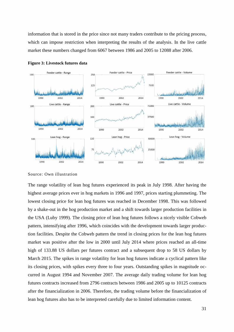
31
information that is stored in the price since not many traders contribute to the pricing process,
which can impose restriction when interpreting the results of the analysis. In the live cattle
market these numbers changed from 6067 between 1986 and 2005 to 12088 after 2006.
Figure 3: Livestock futures data
Source: Own illustration
The range volatility of lean hog futures experienced its peak in July 1998. After having the
highest average prices ever in hog markets in 1996 and 1997, prices starting plummeting. The
lowest closing price for lean hog futures was reached in December 1998. This was followed
by a shake-out in the hog production market and a shift towards larger production facilities in
the USA (Luby 1999). The closing price of lean hog futures follows a nicely visible Cobweb
pattern, intensifying after 1996, which coincides with the development towards larger produc-
tion facilities. Despite the Cobweb pattern the trend in closing prices for the lean hog futures
market was positive after the low in 2000 until July 2014 where prices reached an all-time
high of 133.88 US dollars per futures contract and a subsequent drop to 58 US dollars by
March 2015. The spikes in range volatility for lean hog futures indicate a cyclical pattern like
its closing prices, with spikes every three to four years. Outstanding spikes in magnitude oc-
curred in August 1994 and November 2007. The average daily trading volume for lean hog
futures contracts increased from 2796 contracts between 1986 and 2005 up to 10125 contracts
after the financialization in 2006. Therefore, the trading volume before the financialization of
lean hog futures also has to be interpreted carefully due to limited information content.
32
Figure 4 shows the developments of annualized range volatilities, closing prices and trading
volumes for corn, soybeans and wheat futures respectively. In the feed crop futures markets
the first spike in range volatility and closing prices of corn and soybeans appears in July 1988,
which was the year the USA experienced a severe drought, which lasted into the 1990s (Hunt
and Gordon 1991). The trading volume of soybeans shows two extraordinary spikes with
more than 200000 trades in September 1993 and more than 160000 contracts traded in Sep-
tember 1994, which in both cases depicts the soybean harvesting season in the USA. Accord-
ing to FAOSTAT, the soybean harvest in the USA in 1993 decreased by approximately 15 per
cent compared to 1992. In 1994 the production quantity increased by more than 30 per cent. A
grain price shock hit the US markets in 1996, following a drought in 1995 and a rising export
demand for feed grains (Light and Shevlin 1998). The closing price of corn and wheat spiked
that year and the range volatility in the wheat market experienced its peak for the sample pe-
riod in March 1996. In the soybean market the closing price, after a small spike in 1997, de-
clined until 1999, with range volatility spikes in July 1997, July 1998 and July 1999, which in
the USA always depicts the time shortly after soybean planting. In March 2004 the soybean
price spiked, after harvests in South America fell way short of their USDA forecasts (USDA
2006). September 2004 also constituted the month with the range volatility peak in the soy-
bean futures market for the sample period. These developments also coincide with the acces-
sion of China to the WTO in late 2001 and its quick surges in soybean imports. In the corn
market the range volatility peak for the sample period was on 14.09.2004, which is the day the
USDA Feed Outlook for 2004 was published, announcing corn production volume records for
that year (USDA 2004). The peak in range volatility was accompanied by a spike in trading
volume that same day. On May 8th
in 2003 the European Union introduced its Directive
2003/30/EC, announcing that until 2010 a mandatory blending in of biofuels into ordinary
fuels up to 5.75 per cent had to be reached. This announcement was followed by a short spike
in range volatility in the corn futures market during those days. Similar actions can be ob-
served after the introduction of the Energy Policy Act in July 2005 in the USA, announcing
mandatory increases in bioethanol production levels. The commodity price crisis in 2008 lead
to price spikes and range volatility spikes in all three markets. For wheat, the closing price
dropped quickly and afterwards did not return to the crisis levels, whereas for corn and soy-
beans closing prices even surpassed the crisis spikes and remained on record levels from July
2011 until July 2014 for soybeans and from August 2010 until July 2013 for corn. Corn prices
reached their highest level in August 2012 during a major drought in the USA. The drought of
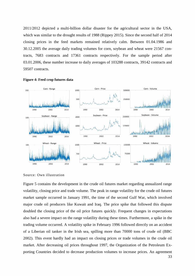
33
2011/2012 depicted a multi-billion dollar disaster for the agricultural sector in the USA,
which was similar to the drought results of 1988 (Rippey 2015). Since the second half of 2014
closing prices in the feed markets remained relatively calm. Between 01.04.1986 and
30.12.2005 the average daily trading volumes for corn, soybean and wheat were 21567 con-
tracts, 7683 contracts and 17361 contracts respectively. For the sample period after
03.01.2006, these number increase to daily averages of 103288 contracts, 39142 contracts and
59507 contracts.
Figure 4: Feed crop futures data
Source: Own illustration
Figure 5 contains the development in the crude oil futures market regarding annualized range
volatility, closing price and trade volume. The peak in range volatility for the crude oil futures
market sample occurred in January 1991, the time of the second Gulf War, which involved
major crude oil producers like Kuwait and Iraq. The price spike that followed this dispute
doubled the closing price of the oil price futures quickly. Frequent changes in expectations
also had a severe impact on the range volatility during these times. Furthermore, a spike in the
trading volume occurred. A volatility spike in February 1996 followed directly on an accident
of a Liberian oil tanker in the Irish sea, spilling more than 70000 tons of crude oil (BBC
2002). This event hardly had an impact on closing prices or trade volumes in the crude oil
market. After decreasing oil prices throughout 1997, the Organization of the Petroleum Ex-
porting Countries decided to decrease production volumes to increase prices. An agreement
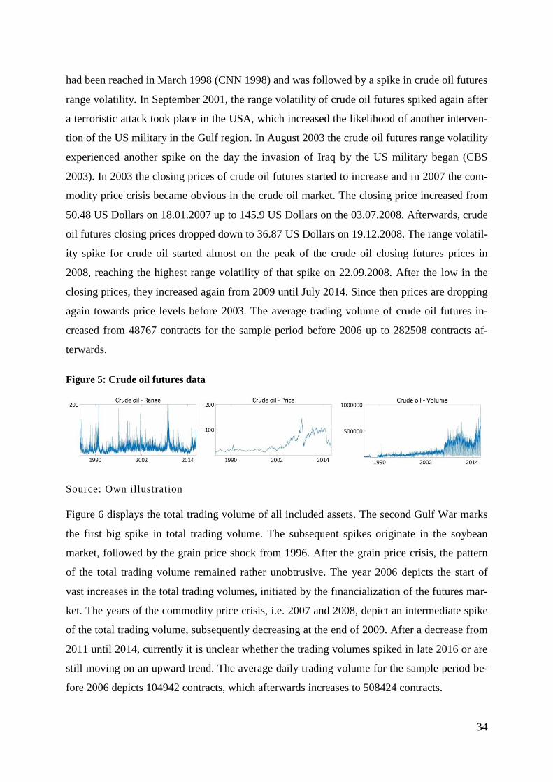
34
had been reached in March 1998 (CNN 1998) and was followed by a spike in crude oil futures
range volatility. In September 2001, the range volatility of crude oil futures spiked again after
a terroristic attack took place in the USA, which increased the likelihood of another interven-
tion of the US military in the Gulf region. In August 2003 the crude oil futures range volatility
experienced another spike on the day the invasion of Iraq by the US military began (CBS
2003). In 2003 the closing prices of crude oil futures started to increase and in 2007 the com-
modity price crisis became obvious in the crude oil market. The closing price increased from
50.48 US Dollars on 18.01.2007 up to 145.9 US Dollars on the 03.07.2008. Afterwards, crude
oil futures closing prices dropped down to 36.87 US Dollars on 19.12.2008. The range volatil-
ity spike for crude oil started almost on the peak of the crude oil closing futures prices in
2008, reaching the highest range volatility of that spike on 22.09.2008. After the low in the
closing prices, they increased again from 2009 until July 2014. Since then prices are dropping
again towards price levels before 2003. The average trading volume of crude oil futures in-
creased from 48767 contracts for the sample period before 2006 up to 282508 contracts af-
terwards.
Figure 5: Crude oil futures data
Source: Own illustration
Figure 6 displays the total trading volume of all included assets. The second Gulf War marks
the first big spike in total trading volume. The subsequent spikes originate in the soybean
market, followed by the grain price shock from 1996. After the grain price crisis, the pattern
of the total trading volume remained rather unobtrusive. The year 2006 depicts the start of
vast increases in the total trading volumes, initiated by the financialization of the futures mar-
ket. The years of the commodity price crisis, i.e. 2007 and 2008, depict an intermediate spike
of the total trading volume, subsequently decreasing at the end of 2009. After a decrease from
2011 until 2014, currently it is unclear whether the trading volumes spiked in late 2016 or are
still moving on an upward trend. The average daily trading volume for the sample period be-
fore 2006 depicts 104942 contracts, which afterwards increases to 508424 contracts.
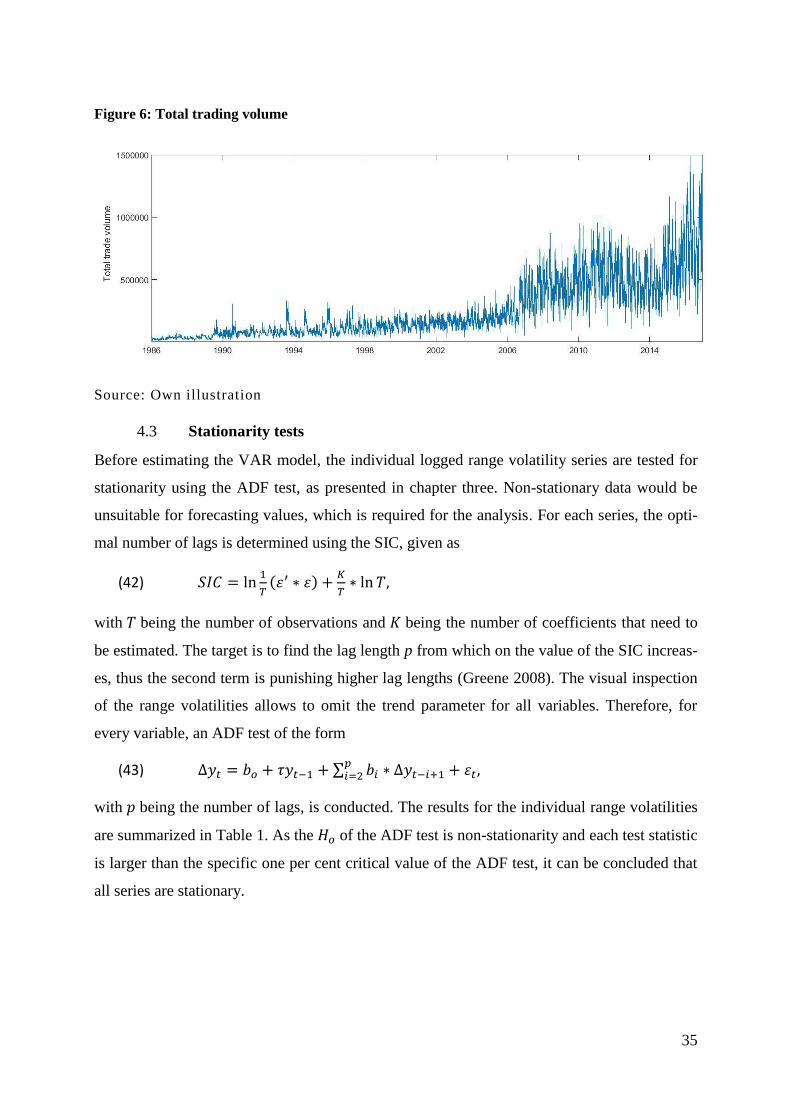
35
Figure 6: Total trading volume
Source: Own illustration
Stationarity tests 4.3
Before estimating the VAR model, the individual logged range volatility series are tested for
stationarity using the ADF test, as presented in chapter three. Non-stationary data would be
unsuitable for forecasting values, which is required for the analysis. For each series, the opti-
mal number of lags is determined using the SIC, given as
(42)
( )
with being the number of observations and being the number of coefficients that need to
be estimated. The target is to find the lag length p from which on the value of the SIC increas-
es, thus the second term is punishing higher lag lengths (Greene 2008). The visual inspection
of the range volatilities allows to omit the trend parameter for all variables. Therefore, for
every variable, an ADF test of the form
(43) ∑ ,
with being the number of lags, is conducted. The results for the individual range volatilities
are summarized in Table 1. As the of the ADF test is non-stationarity and each test statistic
is larger than the specific one per cent critical value of the ADF test, it can be concluded that
all series are stationary.
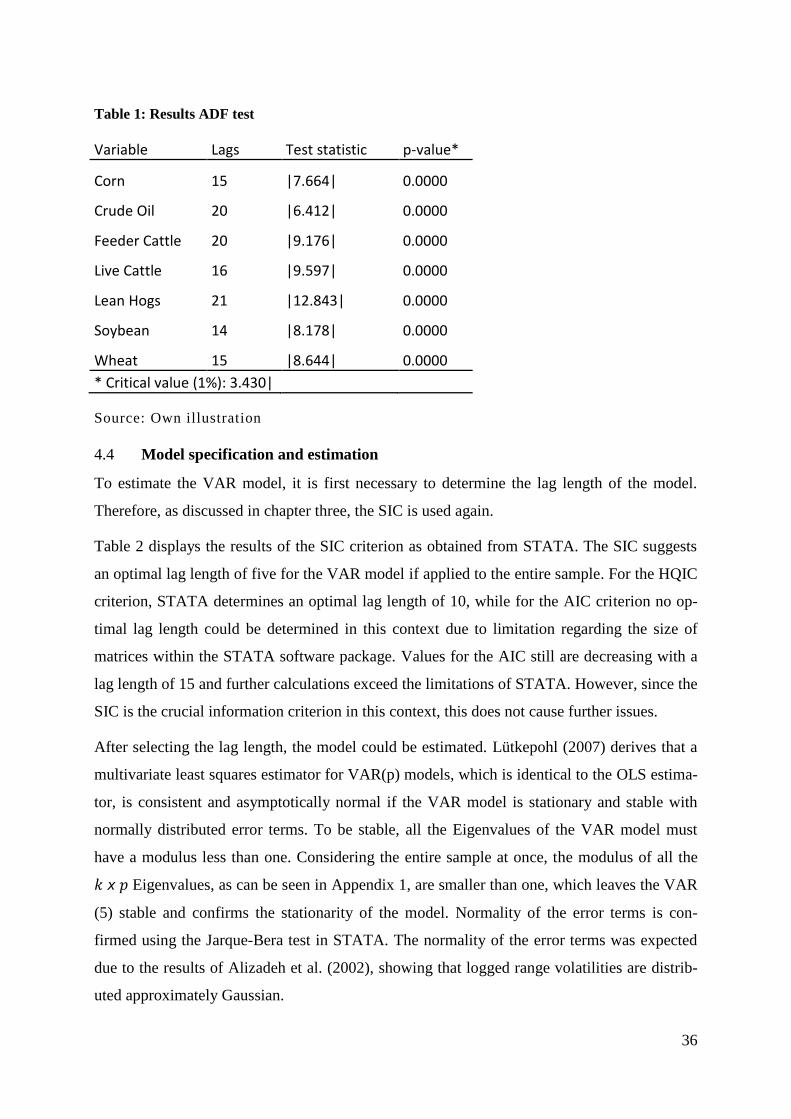
36
Table 1: Results ADF test
Variable Lags Test statistic p-value*
Corn 15 |7.664| 0.0000
Crude Oil 20 |6.412| 0.0000
Feeder Cattle 20 |9.176| 0.0000
Live Cattle 16 |9.597| 0.0000
Lean Hogs 21 |12.843| 0.0000
Soybean 14 |8.178| 0.0000
Wheat 15 |8.644| 0.0000
* Critical value (1%): 3.430|
Source: Own illustration
Model specification and estimation 4.4
To estimate the VAR model, it is first necessary to determine the lag length of the model.
Therefore, as discussed in chapter three, the SIC is used again.
Table 2 displays the results of the SIC criterion as obtained from STATA. The SIC suggests
an optimal lag length of five for the VAR model if applied to the entire sample. For the HQIC
criterion, STATA determines an optimal lag length of 10, while for the AIC criterion no op-
timal lag length could be determined in this context due to limitation regarding the size of
matrices within the STATA software package. Values for the AIC still are decreasing with a
lag length of 15 and further calculations exceed the limitations of STATA. However, since the
SIC is the crucial information criterion in this context, this does not cause further issues.
After selecting the lag length, the model could be estimated. Lütkepohl (2007) derives that a
multivariate least squares estimator for VAR(p) models, which is identical to the OLS estima-
tor, is consistent and asymptotically normal if the VAR model is stationary and stable with
normally distributed error terms. To be stable, all the Eigenvalues of the VAR model must
have a modulus less than one. Considering the entire sample at once, the modulus of all the
Eigenvalues, as can be seen in Appendix 1, are smaller than one, which leaves the VAR
(5) stable and confirms the stationarity of the model. Normality of the error terms is con-
firmed using the Jarque-Bera test in STATA. The normality of the error terms was expected
due to the results of Alizadeh et al. (2002), showing that logged range volatilities are distrib-
uted approximately Gaussian.
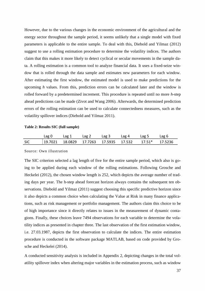
37
However, due to the various changes in the economic environment of the agricultural and the
energy sector throughout the sample period, it seems unlikely that a single model with fixed
parameters is applicable to the entire sample. To deal with this, Diebold and Yilmaz (2012)
suggest to use a rolling estimation procedure to determine the volatility indices. The authors
claim that this makes it more likely to detect cyclical or secular movements in the sample da-
ta. A rolling estimation is a common tool to analyze financial data. It uses a fixed-seize win-
dow that is rolled through the data sample and estimates new parameters for each window.
After estimating the first window, the estimated model is used to make predictions for the
upcoming h values. From this, prediction errors can be calculated later and the window is
rolled forward by a predetermined increment. This procedure is repeated until no more h-step
ahead predictions can be made (Zivot and Wang 2006). Afterwards, the determined prediction
errors of the rolling estimation can be used to calculate connectedness measures, such as the
volatility spillover indices (Diebold and Yilmaz 2011).
Table 2: Results SIC (full sample)
Lag 0 Lag 1 Lag 2 Lag 3 Lag 4 Lag 5 Lag 6
SIC 19.7021 18.0829 17.7263 17.5935 17.532 17.51* 17.5236
Source: Own illustration
The SIC criterion selected a lag length of five for the entire sample period, which also is go-
ing to be applied during each window of the rolling estimations. Following Grosche and
Heckelei (2012), the chosen window length is 252, which depicts the average number of trad-
ing days per year. The h-step ahead forecast horizon always contains the subsequent ten ob-
servations. Diebold and Yilmaz (2011) suggest choosing this specific predictive horizon since
it also depicts a common choice when calculating the Value at Risk in many finance applica-
tions, such as risk management or portfolio management. The authors claim this choice to be
of high importance since it directly relates to issues in the measurement of dynamic conta-
gions. Finally, these choices leave 7494 observations for each variable to determine the vola-
tility indices as presented in chapter three. The last observation of the first estimation window,
i.e. 27.03.1987, depicts the first observation to calculate the indices. The entire estimation
procedure is conducted in the software package MATLAB, based on code provided by Gro-
sche and Heckelei (2014).
A conducted sensitivity analysis is included in Appendix 2, depicting changes in the total vol-
atility spillover index when altering major variables in the estimation process, such as window

38
size or lag length. The biggest differences occur when reducing the window size by half, shift-
ing the total volatility spillover index significantly upward, while excluding crude oil futures
from the analysis only has very minor impacts on the results.
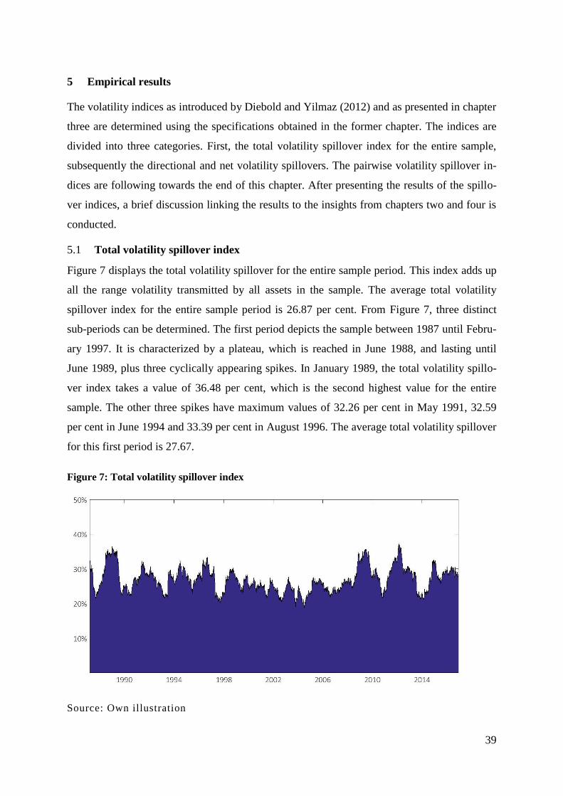
39
5 Empirical results
The volatility indices as introduced by Diebold and Yilmaz (2012) and as presented in chapter
three are determined using the specifications obtained in the former chapter. The indices are
divided into three categories. First, the total volatility spillover index for the entire sample,
subsequently the directional and net volatility spillovers. The pairwise volatility spillover in-
dices are following towards the end of this chapter. After presenting the results of the spillo-
ver indices, a brief discussion linking the results to the insights from chapters two and four is
conducted.
Total volatility spillover index 5.1
Figure 7 displays the total volatility spillover for the entire sample period. This index adds up
all the range volatility transmitted by all assets in the sample. The average total volatility
spillover index for the entire sample period is 26.87 per cent. From Figure 7, three distinct
sub-periods can be determined. The first period depicts the sample between 1987 until Febru-
ary 1997. It is characterized by a plateau, which is reached in June 1988, and lasting until
June 1989, plus three cyclically appearing spikes. In January 1989, the total volatility spillo-
ver index takes a value of 36.48 per cent, which is the second highest value for the entire
sample. The other three spikes have maximum values of 32.26 per cent in May 1991, 32.59
per cent in June 1994 and 33.39 per cent in August 1996. The average total volatility spillover
for this first period is 27.67.
Figure 7: Total volatility spillover index
Source: Own illustration
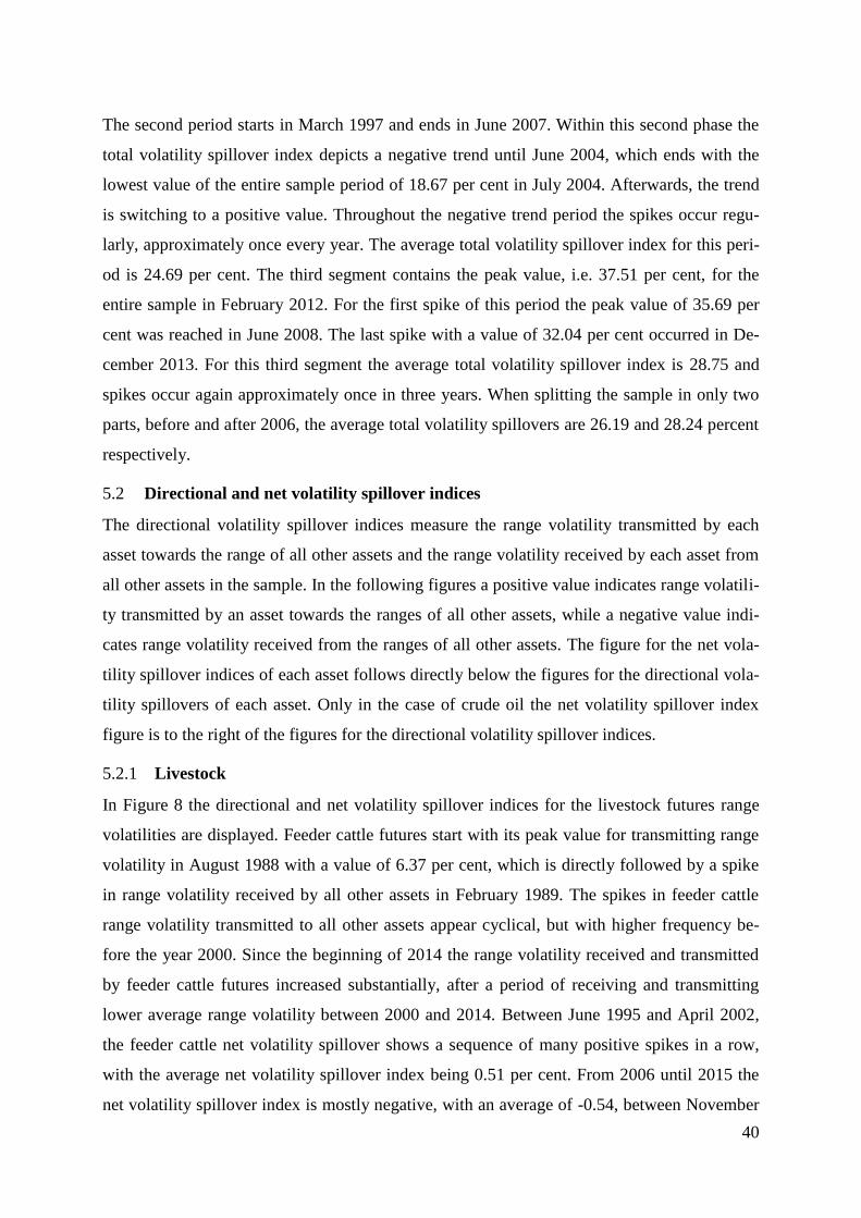
40
The second period starts in March 1997 and ends in June 2007. Within this second phase the
total volatility spillover index depicts a negative trend until June 2004, which ends with the
lowest value of the entire sample period of 18.67 per cent in July 2004. Afterwards, the trend
is switching to a positive value. Throughout the negative trend period the spikes occur regu-
larly, approximately once every year. The average total volatility spillover index for this peri-
od is 24.69 per cent. The third segment contains the peak value, i.e. 37.51 per cent, for the
entire sample in February 2012. For the first spike of this period the peak value of 35.69 per
cent was reached in June 2008. The last spike with a value of 32.04 per cent occurred in De-
cember 2013. For this third segment the average total volatility spillover index is 28.75 and
spikes occur again approximately once in three years. When splitting the sample in only two
parts, before and after 2006, the average total volatility spillovers are 26.19 and 28.24 percent
respectively.
Directional and net volatility spillover indices 5.2
The directional volatility spillover indices measure the range volatility transmitted by each
asset towards the range of all other assets and the range volatility received by each asset from
all other assets in the sample. In the following figures a positive value indicates range volatili-
ty transmitted by an asset towards the ranges of all other assets, while a negative value indi-
cates range volatility received from the ranges of all other assets. The figure for the net vola-
tility spillover indices of each asset follows directly below the figures for the directional vola-
tility spillovers of each asset. Only in the case of crude oil the net volatility spillover index
figure is to the right of the figures for the directional volatility spillover indices.
5.2.1 Livestock
In Figure 8 the directional and net volatility spillover indices for the livestock futures range
volatilities are displayed. Feeder cattle futures start with its peak value for transmitting range
volatility in August 1988 with a value of 6.37 per cent, which is directly followed by a spike
in range volatility received by all other assets in February 1989. The spikes in feeder cattle
range volatility transmitted to all other assets appear cyclical, but with higher frequency be-
fore the year 2000. Since the beginning of 2014 the range volatility received and transmitted
by feeder cattle futures increased substantially, after a period of receiving and transmitting
lower average range volatility between 2000 and 2014. Between June 1995 and April 2002,
the feeder cattle net volatility spillover shows a sequence of many positive spikes in a row,
with the average net volatility spillover index being 0.51 per cent. From 2006 until 2015 the
net volatility spillover index is mostly negative, with an average of -0.54, between November
41
2011 and June 2013 the average goes down to -1.1 per cent. In total feeder cattle is a net range
volatility receiver from all other assets.
Figure 8: Livestock directional and net spillover indices
Source: Own illustration
Live cattle futures are a net range volatility receiver and even more so than feeder cattle fu-
tures, especially within the periods between January 1998 until March 2004 with an average
value of -0.74 per cent and between November 2003 and September 2014 with the average
value of -0.46 per cent. The spikes in range volatility received and transmitted by all other
assets show a cyclical pattern. A very steep increase in range volatility transmitted to all other
assets occurred in April 1994, reaching the sample period peak in August 1994 with a value of
7.44 per cent. Spikes in live cattle range volatility transmission occur approximately every 3.5
years. Range volatility received by the range volatility of live cattle futures peaked twice with
a value of 6.2 per cent, first in January 1989 and then in February 1992.
Lean hog futures range volatility transmitted to all other assets peaked in November 1988
with a value of 5.43 per cent. This peak in range volatility transmitted is accompanied by a
peak in range volatility received, which repeats itself in May 1991. The peak of range volatili-
ty received from all other assets for the entire sample period occurs in October 2014. Over the
entire sample period the average range volatility transmitted by lean hog futures to all other
assets is as low as 2.32 per cent, while for feeder cattle and live cattle these values were 3.49
per cent and 3.69 per cent respectively. In total, lean hog futures are a net receiver of range
volatility like the other livestock futures range volatilities. Its total value approaches the value
of live cattle and is thus higher than the value for feeder cattle.
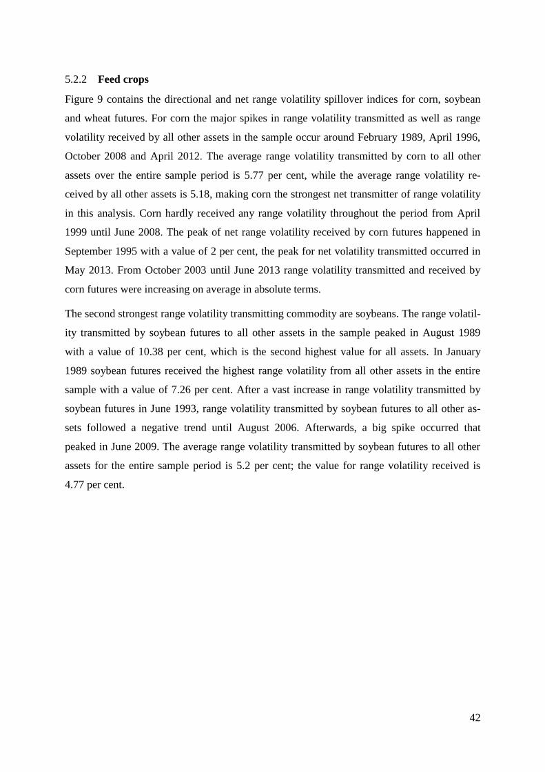
42
5.2.2 Feed crops
Figure 9 contains the directional and net range volatility spillover indices for corn, soybean
and wheat futures. For corn the major spikes in range volatility transmitted as well as range
volatility received by all other assets in the sample occur around February 1989, April 1996,
October 2008 and April 2012. The average range volatility transmitted by corn to all other
assets over the entire sample period is 5.77 per cent, while the average range volatility re-
ceived by all other assets is 5.18, making corn the strongest net transmitter of range volatility
in this analysis. Corn hardly received any range volatility throughout the period from April
1999 until June 2008. The peak of net range volatility received by corn futures happened in
September 1995 with a value of 2 per cent, the peak for net volatility transmitted occurred in
May 2013. From October 2003 until June 2013 range volatility transmitted and received by
corn futures were increasing on average in absolute terms.
The second strongest range volatility transmitting commodity are soybeans. The range volatil-
ity transmitted by soybean futures to all other assets in the sample peaked in August 1989
with a value of 10.38 per cent, which is the second highest value for all assets. In January
1989 soybean futures received the highest range volatility from all other assets in the entire
sample with a value of 7.26 per cent. After a vast increase in range volatility transmitted by
soybean futures in June 1993, range volatility transmitted by soybean futures to all other as-
sets followed a negative trend until August 2006. Afterwards, a big spike occurred that
peaked in June 2009. The average range volatility transmitted by soybean futures to all other
assets for the entire sample period is 5.2 per cent; the value for range volatility received is
4.77 per cent.
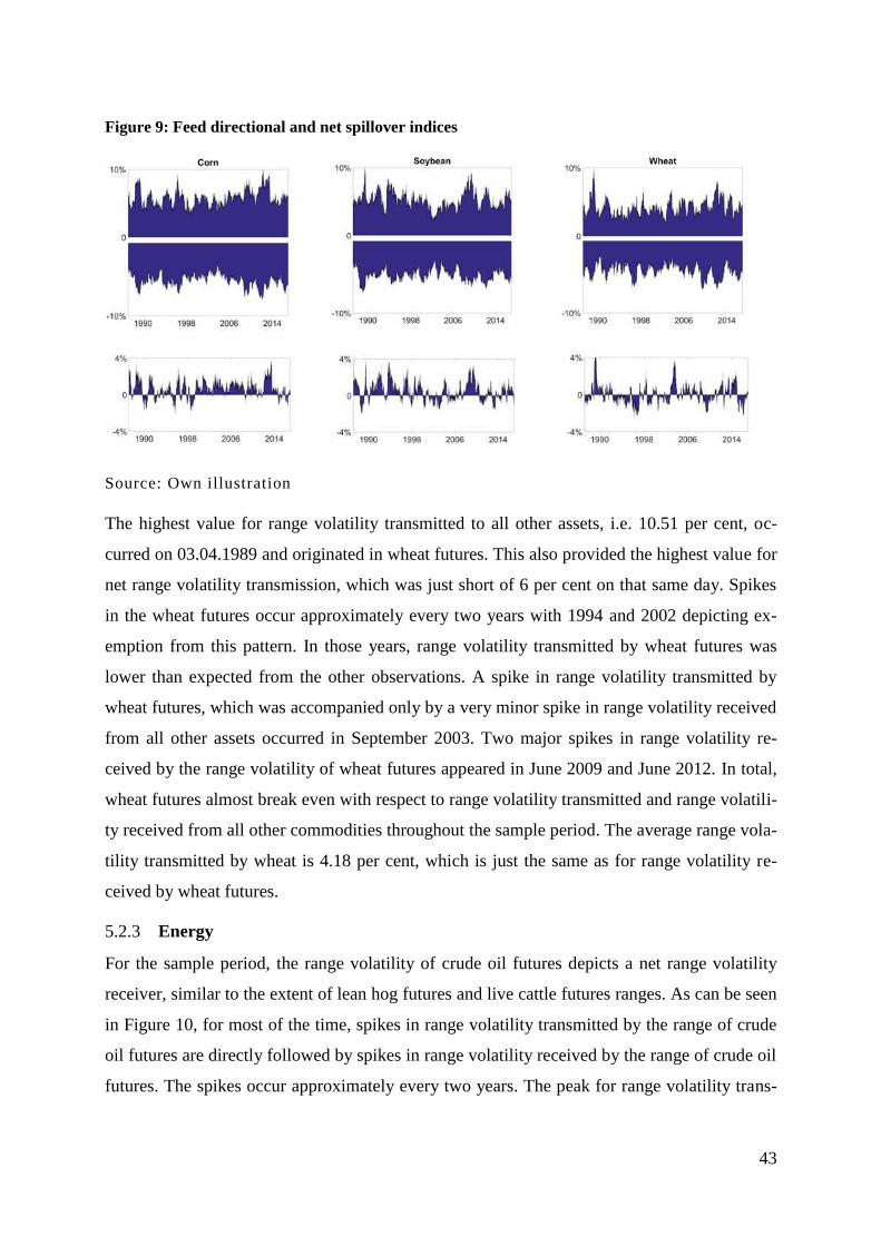
43
Figure 9: Feed directional and net spillover indices
Source: Own illustration
The highest value for range volatility transmitted to all other assets, i.e. 10.51 per cent, oc-
curred on 03.04.1989 and originated in wheat futures. This also provided the highest value for
net range volatility transmission, which was just short of 6 per cent on that same day. Spikes
in the wheat futures occur approximately every two years with 1994 and 2002 depicting ex-
emption from this pattern. In those years, range volatility transmitted by wheat futures was
lower than expected from the other observations. A spike in range volatility transmitted by
wheat futures, which was accompanied only by a very minor spike in range volatility received
from all other assets occurred in September 2003. Two major spikes in range volatility re-
ceived by the range volatility of wheat futures appeared in June 2009 and June 2012. In total,
wheat futures almost break even with respect to range volatility transmitted and range volatili-
ty received from all other commodities throughout the sample period. The average range vola-
tility transmitted by wheat is 4.18 per cent, which is just the same as for range volatility re-
ceived by wheat futures.
5.2.3 Energy
For the sample period, the range volatility of crude oil futures depicts a net range volatility
receiver, similar to the extent of lean hog futures and live cattle futures ranges. As can be seen
in Figure 10, for most of the time, spikes in range volatility transmitted by the range of crude
oil futures are directly followed by spikes in range volatility received by the range of crude oil
futures. The spikes occur approximately every two years. The peak for range volatility trans-
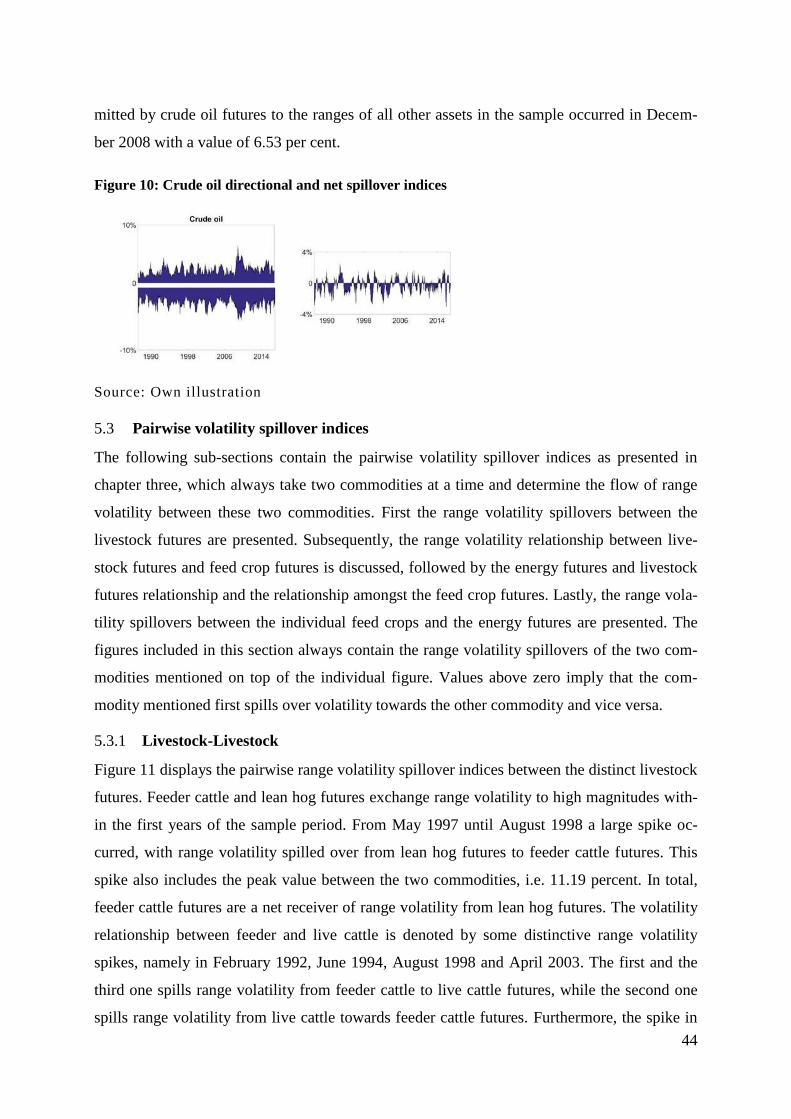
44
mitted by crude oil futures to the ranges of all other assets in the sample occurred in Decem-
ber 2008 with a value of 6.53 per cent.
Figure 10: Crude oil directional and net spillover indices
Source: Own illustration
Pairwise volatility spillover indices 5.3
The following sub-sections contain the pairwise volatility spillover indices as presented in
chapter three, which always take two commodities at a time and determine the flow of range
volatility between these two commodities. First the range volatility spillovers between the
livestock futures are presented. Subsequently, the range volatility relationship between live-
stock futures and feed crop futures is discussed, followed by the energy futures and livestock
futures relationship and the relationship amongst the feed crop futures. Lastly, the range vola-
tility spillovers between the individual feed crops and the energy futures are presented. The
figures included in this section always contain the range volatility spillovers of the two com-
modities mentioned on top of the individual figure. Values above zero imply that the com-
modity mentioned first spills over volatility towards the other commodity and vice versa.
5.3.1 Livestock-Livestock
Figure 11 displays the pairwise range volatility spillover indices between the distinct livestock
futures. Feeder cattle and lean hog futures exchange range volatility to high magnitudes with-
in the first years of the sample period. From May 1997 until August 1998 a large spike oc-
curred, with range volatility spilled over from lean hog futures to feeder cattle futures. This
spike also includes the peak value between the two commodities, i.e. 11.19 percent. In total,
feeder cattle futures are a net receiver of range volatility from lean hog futures. The volatility
relationship between feeder and live cattle is denoted by some distinctive range volatility
spikes, namely in February 1992, June 1994, August 1998 and April 2003. The first and the
third one spills range volatility from feeder cattle to live cattle futures, while the second one
spills range volatility from live cattle towards feeder cattle futures. Furthermore, the spike in
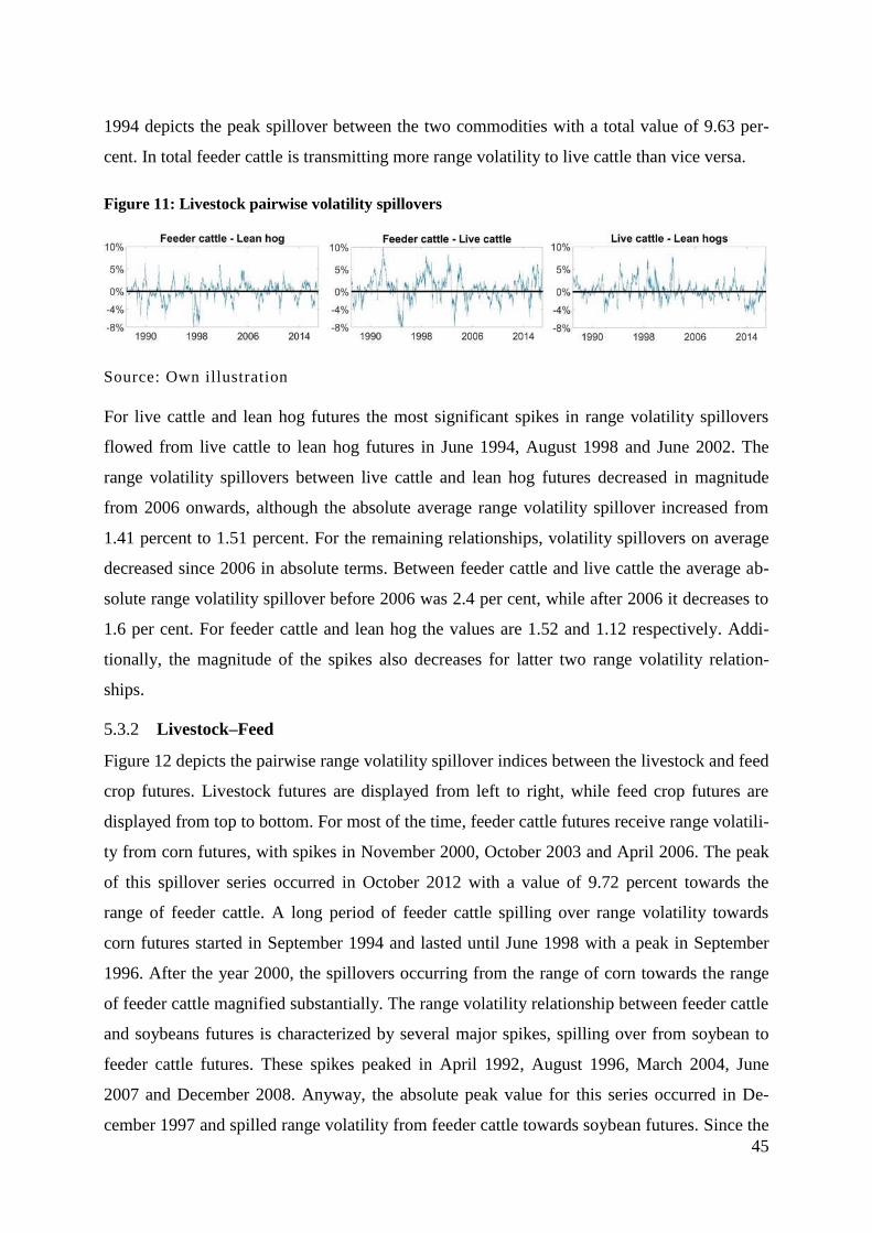
45
1994 depicts the peak spillover between the two commodities with a total value of 9.63 per-
cent. In total feeder cattle is transmitting more range volatility to live cattle than vice versa.
Figure 11: Livestock pairwise volatility spillovers
Source: Own illustration
For live cattle and lean hog futures the most significant spikes in range volatility spillovers
flowed from live cattle to lean hog futures in June 1994, August 1998 and June 2002. The
range volatility spillovers between live cattle and lean hog futures decreased in magnitude
from 2006 onwards, although the absolute average range volatility spillover increased from
1.41 percent to 1.51 percent. For the remaining relationships, volatility spillovers on average
decreased since 2006 in absolute terms. Between feeder cattle and live cattle the average ab-
solute range volatility spillover before 2006 was 2.4 per cent, while after 2006 it decreases to
1.6 per cent. For feeder cattle and lean hog the values are 1.52 and 1.12 respectively. Addi-
tionally, the magnitude of the spikes also decreases for latter two range volatility relation-
ships.
5.3.2 Livestock–Feed
Figure 12 depicts the pairwise range volatility spillover indices between the livestock and feed
crop futures. Livestock futures are displayed from left to right, while feed crop futures are
displayed from top to bottom. For most of the time, feeder cattle futures receive range volatili-
ty from corn futures, with spikes in November 2000, October 2003 and April 2006. The peak
of this spillover series occurred in October 2012 with a value of 9.72 percent towards the
range of feeder cattle. A long period of feeder cattle spilling over range volatility towards
corn futures started in September 1994 and lasted until June 1998 with a peak in September
1996. After the year 2000, the spillovers occurring from the range of corn towards the range
of feeder cattle magnified substantially. The range volatility relationship between feeder cattle
and soybeans futures is characterized by several major spikes, spilling over from soybean to
feeder cattle futures. These spikes peaked in April 1992, August 1996, March 2004, June
2007 and December 2008. Anyway, the absolute peak value for this series occurred in De-
cember 1997 and spilled range volatility from feeder cattle towards soybean futures. Since the
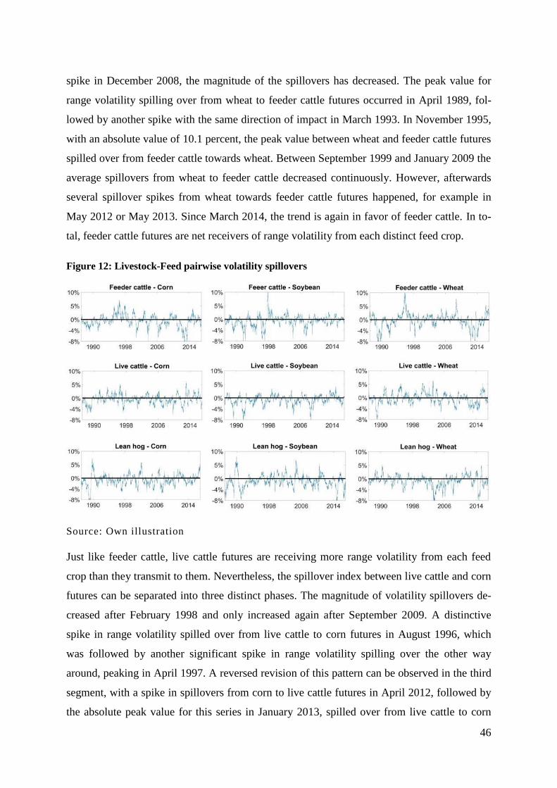
46
spike in December 2008, the magnitude of the spillovers has decreased. The peak value for
range volatility spilling over from wheat to feeder cattle futures occurred in April 1989, fol-
lowed by another spike with the same direction of impact in March 1993. In November 1995,
with an absolute value of 10.1 percent, the peak value between wheat and feeder cattle futures
spilled over from feeder cattle towards wheat. Between September 1999 and January 2009 the
average spillovers from wheat to feeder cattle decreased continuously. However, afterwards
several spillover spikes from wheat towards feeder cattle futures happened, for example in
May 2012 or May 2013. Since March 2014, the trend is again in favor of feeder cattle. In to-
tal, feeder cattle futures are net receivers of range volatility from each distinct feed crop.
Figure 12: Livestock-Feed pairwise volatility spillovers
Source: Own illustration
Just like feeder cattle, live cattle futures are receiving more range volatility from each feed
crop than they transmit to them. Nevertheless, the spillover index between live cattle and corn
futures can be separated into three distinct phases. The magnitude of volatility spillovers de-
creased after February 1998 and only increased again after September 2009. A distinctive
spike in range volatility spilled over from live cattle to corn futures in August 1996, which
was followed by another significant spike in range volatility spilling over the other way
around, peaking in April 1997. A reversed revision of this pattern can be observed in the third
segment, with a spike in spillovers from corn to live cattle futures in April 2012, followed by
the absolute peak value for this series in January 2013, spilled over from live cattle to corn

47
futures range volatility. From soybean futures, live cattle futures are receiving range volatility
almost all the time in the sample period. The most significant spikes for range volatility spill-
overs from soybean to live cattle futures happened in June 1989, November 1991, April 2004
and August 2008. The value in August 2008, i.e. 8.25 percent in absolute terms, depicts the
peak of this series. The relationship with wheat futures is not as one-sided for live cattle as it
is with soybean futures. April 1989 depicts the peak value for this series, spilling over from
wheat to live cattle futures. Afterwards, a period of range volatility mainly spilling over from
live cattle towards wheat futures started in June 1990 and lasted approximately until June
2004. Throughout this distinct period live cattle is spilling over more range volatility towards
wheat than vice versa.
The range volatility relationship between lean hog, corn and soybean futures is characterized
by peaks in the beginning of the sample period. The range volatility spillover from corn into
lean hog futures peaked in April 1989 with the reversed spillover peak in December 1989.
With soybean these values have been reached in June 1989 and January 1990 respectively.
Another significant spike of range volatility spilling over from lean hog to corn futures oc-
curred in April 2002. Distinctive spikes from corn to lean hog futures happened in April 1997,
April 2001, July 2003, March 2005 and June 2007. Range volatility spilled from lean hog to
soybean futures spiked in September 2004 and July 2010. In recent years volatility spillovers
from soybean to lean hog futures spiked in October 2014 and January 2016. Regarding wheat,
lean hog futures mostly receive range volatility. The peak spillover from wheat to lean hog
futures happened in August 2003 with an absolute value of 13.8 percent. Another major spill-
over in this direction occurred in September 2014 with an absolute value of 10.2 percent. A
trend towards less range volatility spillover flowing from wheat towards lean hog futures can
be detected in the period between September 2003 and April 2011.
5.3.3 Energy–Livestock
Figure 13 depicts the pairwise range volatility spillover indices between crude oil and live-
stock futures. Crude oil transmits more range volatility towards both the cattle futures than it
receives from them, but vice versa for its relationship with lean hog futures. For none of the
relationships distinct changes in spillover patterns can be detected for the sample period.
Feeder cattle futures spill over high levels of range volatility to crude oil futures in April
1988, April 2002 and just recently in August 2016. The other way around, spikes occurred in
August 1995, October 2003, August 2008 and July 2015. Live cattle futures spill over large
chunks of range volatility towards crude oil futures in April 2002 and September 2014. The
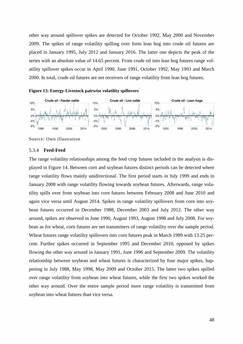
48
other way around spillover spikes are detected for October 1992, May 2000 and November
2009. The spikes of range volatility spilling over form lean hog into crude oil futures are
placed in January 1995, July 2012 and January 2016. The latter one depicts the peak of the
series with an absolute value of 14.65 percent. From crude oil into lean hog futures range vol-
atility spillover spikes occur in April 1990, June 1991, October 1992, May 1993 and March
2000. In total, crude oil futures are net receivers of range volatility from lean hog futures.
Figure 13: Energy-Livestock pairwise volatility spillovers
Source: Own illustration
5.3.4 Feed-Feed
The range volatility relationships among the feed crop futures included in the analysis is dis-
played in Figure 14. Between corn and soybean futures distinct periods can be detected where
range volatility flows mainly unidirectional. The first period starts in July 1999 and ends in
January 2008 with range volatility flowing towards soybean futures. Afterwards, range vola-
tility spills over from soybean into corn futures between February 2008 and June 2010 and
again vice versa until August 2014. Spikes in range volatility spillovers from corn into soy-
bean futures occurred in December 1988, December 2003 and July 2012. The other way
around, spikes are observed in June 1990, August 1993, August 1998 and July 2008. For soy-
bean as for wheat, corn futures are net transmitters of range volatility over the sample period.
Wheat futures range volatility spillovers into corn futures peak in March 1989 with 13.25 per-
cent. Further spikes occurred in September 1995 and December 2010, opposed by spikes
flowing the other way around in January 1991, June 1996 and September 2009. The volatility
relationship between soybean and wheat futures is characterized by four major spikes, hap-
pening in July 1988, May 1998, May 2009 and October 2015. The latter two spikes spilled
over range volatility from soybean into wheat futures, while the first two spikes worked the
other way around. Over the entire sample period more range volatility is transmitted from
soybean into wheat futures than vice versa.
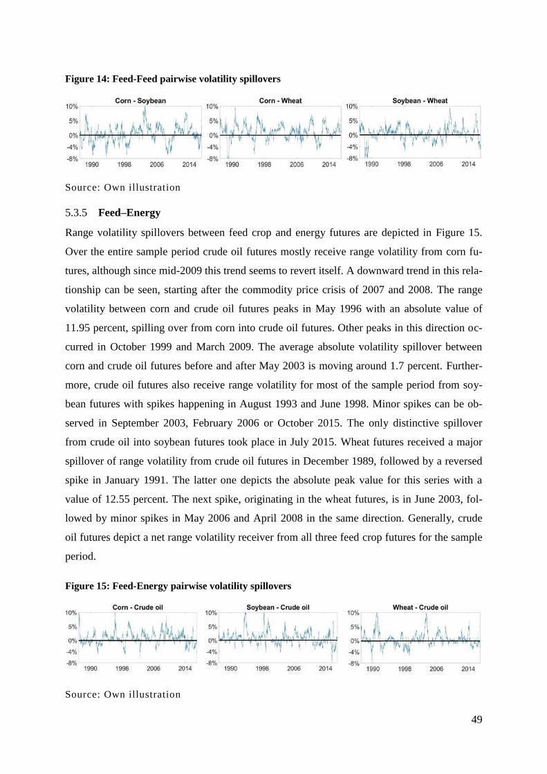
49
Figure 14: Feed-Feed pairwise volatility spillovers
Source: Own illustration
5.3.5 Feed–Energy
Range volatility spillovers between feed crop and energy futures are depicted in Figure 15.
Over the entire sample period crude oil futures mostly receive range volatility from corn fu-
tures, although since mid-2009 this trend seems to revert itself. A downward trend in this rela-
tionship can be seen, starting after the commodity price crisis of 2007 and 2008. The range
volatility between corn and crude oil futures peaks in May 1996 with an absolute value of
11.95 percent, spilling over from corn into crude oil futures. Other peaks in this direction oc-
curred in October 1999 and March 2009. The average absolute volatility spillover between
corn and crude oil futures before and after May 2003 is moving around 1.7 percent. Further-
more, crude oil futures also receive range volatility for most of the sample period from soy-
bean futures with spikes happening in August 1993 and June 1998. Minor spikes can be ob-
served in September 2003, February 2006 or October 2015. The only distinctive spillover
from crude oil into soybean futures took place in July 2015. Wheat futures received a major
spillover of range volatility from crude oil futures in December 1989, followed by a reversed
spike in January 1991. The latter one depicts the absolute peak value for this series with a
value of 12.55 percent. The next spike, originating in the wheat futures, is in June 2003, fol-
lowed by minor spikes in May 2006 and April 2008 in the same direction. Generally, crude
oil futures depict a net range volatility receiver from all three feed crop futures for the sample
period.
Figure 15: Feed-Energy pairwise volatility spillovers
Source: Own illustration
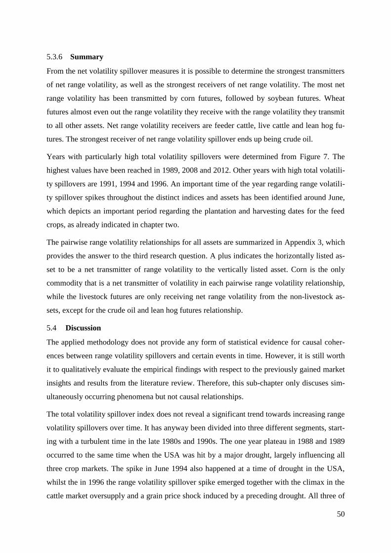
50
5.3.6 Summary
From the net volatility spillover measures it is possible to determine the strongest transmitters
of net range volatility, as well as the strongest receivers of net range volatility. The most net
range volatility has been transmitted by corn futures, followed by soybean futures. Wheat
futures almost even out the range volatility they receive with the range volatility they transmit
to all other assets. Net range volatility receivers are feeder cattle, live cattle and lean hog fu-
tures. The strongest receiver of net range volatility spillover ends up being crude oil.
Years with particularly high total volatility spillovers were determined from Figure 7. The
highest values have been reached in 1989, 2008 and 2012. Other years with high total volatili-
ty spillovers are 1991, 1994 and 1996. An important time of the year regarding range volatili-
ty spillover spikes throughout the distinct indices and assets has been identified around June,
which depicts an important period regarding the plantation and harvesting dates for the feed
crops, as already indicated in chapter two.
The pairwise range volatility relationships for all assets are summarized in Appendix 3, which
provides the answer to the third research question. A plus indicates the horizontally listed as-
set to be a net transmitter of range volatility to the vertically listed asset. Corn is the only
commodity that is a net transmitter of volatility in each pairwise range volatility relationship,
while the livestock futures are only receiving net range volatility from the non-livestock as-
sets, except for the crude oil and lean hog futures relationship.
Discussion 5.4
The applied methodology does not provide any form of statistical evidence for causal coher-
ences between range volatility spillovers and certain events in time. However, it is still worth
it to qualitatively evaluate the empirical findings with respect to the previously gained market
insights and results from the literature review. Therefore, this sub-chapter only discuses sim-
ultaneously occurring phenomena but not causal relationships.
The total volatility spillover index does not reveal a significant trend towards increasing range
volatility spillovers over time. It has anyway been divided into three different segments, start-
ing with a turbulent time in the late 1980s and 1990s. The one year plateau in 1988 and 1989
occurred to the same time when the USA was hit by a major drought, largely influencing all
three crop markets. The spike in June 1994 also happened at a time of drought in the USA,
whilst the in 1996 the range volatility spillover spike emerged together with the climax in the
cattle market oversupply and a grain price shock induced by a preceding drought. All three of
51
these spikes have been accompanied by local highs in the total trading volume. After a ten-
year period of decreasing average total volatility spillovers, the commodity price crisis of
2007 and 2008 hit the markets, characterized by price jumps in crude oil and the feed crops
futures and a big spike in the total range volatility spillover index. The commodity price crisis
has been accompanied by the financialization of the futures markets, but as already mentioned
before might not have been caused by it. The peak in total range volatility spillovers in 2012
evolved around another major drought in the USA, comparable only to the drought in 1988,
which depicts the second highest total volatility spillover index value. The average total vola-
tility spillover index in the third segment is higher than in the first segment, but it also con-
tains a major drought in the USA, the commodity price crisis of 2007 and 2008 and the finan-
cialization of the futures market. Comparing Figure 6 and Figure 7 does not leave a categori-
cal impression on the relationship between market liquidity and total range volatility spillo-
vers since the vast increases in trading volume seem not to have caused an increase of compa-
rable magnitude in total range volatility spillovers. Furthermore, from evaluating the results
with respect to the first research question regarding the relationship between the demand for
feedstock and total volatility spillovers, no evidence can be detected supporting a positive
correlation between these two factors. The reason for this result cannot be pinned down to
single causes, but an important factor is the short-term data used during the analysis relative
to the log-term structural changes underlying the increasing demand for feedstock, which has
been indicated by Gardebroek et al. (2016). The short-term data mostly catches unforeseen
immediate events that directly impact commodity supply and demand, which is represented
best by the frequent spikes evolving around the droughts. Furthermore, the increasing produc-
tion volumes of the feed crops might have prevented increasing pressure on the markets by
sufficiently answering increasing demand with increasing supply.
The directional range volatility indices and the subsequent net directional range volatility
measures reveal corn and soybeans as the major transmitters of volatility in the system, which
comes as no surprise if considering their importance in the American agricultural sector. The
fact that these two commodities are emitting a lot of range volatility translates into the hy-
pothesis that the key drivers influencing these markets are likely to also influence other mar-
kets (Grosche and Heckelei 2014). Additionally, it is noteworthy that the futures with the
highest liquidity are the major range volatility transmitters, not considering crude oil futures.
Therefore, it seems plausible that information is flowing from these central markets into other
subordinate markets in the agricultural market. The spikes in range volatility transmitted by

52
corn futures to all other assets concentrate on the drought years in the USA and the commodi-
ty price crisis. The peak in directional volatility transmitted by soybeans occurred in the
drought year 1989 and also the spike in 1993 was accompanied by a significant decrease in
the total soybean harvest in the USA. Wheat transmitted a lot of range volatility during the
drought of 1989, but in total does not represent a net range volatility transmitter. Severe
droughts inside a major producer like the USA can have significant effects on the future price
expectation of speculators for several commodities in the derivative exchanges due to their
various linkages. Weather is hard to predict accurately and traders need to adjust their price
expectation continuously, even more so in times of extreme weather events that have signifi-
cant effects on production volumes. Therefore, it is no surprise that a lot of information is
exchanged among the markets in times of droughts. The livestock futures hardly transmit net
range volatility to the other assets, despite feeder cattle after the climax of the beef market
oversupply. But they do frequently receive net range volatility spillovers during times of
drought in the USA, which again is not surprising since droughts directly influence the main
input for livestock production and the information regarding changes in the feed markets is
directly processed into the future expectation of traders in the livestock sector. When looking
for patterns in the net directional range volatility indices for the livestock futures no trend
towards more volatility transmission towards other assets can be qualitatively detected in later
periods of the sample.
The pairwise volatility spillovers confirm the scarce results from the literature review regard-
ing volatility spillovers from feed into livestock markets. The results of the studies by Buguk
et al. (2003) and Apergis and Rezitis (2003) both indicate that volatility spills over from feed
into livestock markets, based on GARCH models and spot prices. However, from Figure 12
more detailed insights can be obtained. Feed crop futures are all ultimately net range volatility
transmitters towards livestock futures, but in the mid-1990s feeder cattle futures have trans-
mitted range volatility to each feed market, either in spikes as to soybean and wheat futures or
during an extended time period to corn futures. It would thus be worthwhile to further investi-
gate the implications of the beef market oversupply in the USA during the 1990s for the feed
markets. Speculators might expect production volumes to go down in the cattle market sub-
stantially and thus also expect a decrease in feed demand, which ultimately alters the specula-
tors expectation of future feed crop prices. Problematic for this period is that the trading vol-
umes of feeder cattle futures averages around 700 traded contracts per day, which restricts the
amount of information that is stored in the market. Another interesting observation in the
53
pairwise livestock-feed relationship is the volatility spillover peaks from lean hog futures into
soybean and corn markets in 1989. Figure 3 indicates that 1990 depicted the end of one of the
hog marketing cycles, although it did not have major price effects or range volatility effects
on lean hog futures themselves. Towards the end of a marketing cycle traders could already
assume feed demand to change soon and thus alter their expectations accordingly in the mar-
kets. A lack of data regarding the trade volumes for lean hog and corn futures provides an
obstacle in the interpretation of this situation. It depicts a possibility that the trading volumes
in the lean hog futures market to that time was too thin to actually allow for any meaningful
results since the amount of information stored in the market is not sufficient. Ultimately, Fig-
ure 12 does not provide any evidence for a trend of increasing range volatility spillovers from
livestock futures into feed crop futures throughout the recent decades, although there has been
a positive trend between lean hog and wheat futures between 2003 and 2011. A similar trend
can be observed between feeder cattle and wheat between 1999 and 2009.
Within the feed crop futures markets corn and soybean futures are both net range volatility
transmitters towards wheat futures and corn is a net range volatility transmitter towards soy-
beans. This represents also the ordering in the number of acres devoted to each plant, with
wheat only obtaining half the amount of acres of soybeans and roughly 45 percent of corn
acreage in 2015 (USDA 2016). Anyway, to the time of the first major drought in the USA in
1989, wheat futures spilled over large portions of range volatility towards the other feed
crops. After the 1989 drought soybeans depict a range volatility transmitter towards wheat
futures in times of drought like 1996 or 2012. Corn on the other hand receives range volatility
from wheat futures during these two particular drought years. In non-drought years corn is
mostly transmitting range volatility into wheat futures. The information flow within these
sectors could be influenced by the differences in planting and harvesting dates, which can
allow for years with soybean and wheat production but hardly allows for wheat and corn pro-
duction combined. Furthermore, corn as the strongest volatility depicts the most liquid market
with the most information stored in its price. The liquidity of the soybean futures market is
lower than the liquidity in the wheat market, translating into information being transmitted
from the less informed market into the market with higher information content.
Looking into the pairwise range volatility relationships of crude oil futures does not allow for
conclusive statements on the impact of developments within the energy sector on the infor-
mation flow between it and its related markets. Just in recent times all three livestock futures
transmitted significant spikes of range volatility into the crude oil futures market. Lean hog
54
futures even constitute a net range volatility transmitter towards crude oil futures, although,
this result has to be considered in the light of the large differences of the trading volumes be-
tween the two markets. The information concentrated in the livestock futures only constitutes
a fraction of the information stored in the crude oil market. The counterintuitive result from
the analysis that information is transmitted from livestock markets into the crude oil market,
especially before the financialization of the futures market might be a result of this large dif-
ference. Further investigation on this matter is required to make more decisive statements.
The downward trend for range volatility spillovers specifically from corn into crude oil fu-
tures since the end of the commodity price crisis could be a result of the biofuel sector devel-
opments and the linkages that have been created by it. This would be in line with the return-
based GARCH model results of Guan et al. (2011) in so far as a trend towards increasing vol-
atility spillovers from crude oil into corn markets can be detected in recent times. The results
of the analysis contradict the findings of Nazlioglu et al. (2013) and Gilbert and Mugera
(2014), based on GARCH models and return volatility, in so far that during the crisis range
volatility spilled over from corn into crude oil futures and not vice versa. Furthermore, the
results of the analysis contradict the results of the literature review regarding the direction of
the information flow between corn and crude oil futures. In this set-up, the latter is a net range
volatility receiver from corn futures and not a transmitter of volatility. Range volatility spikes
from crude oil into corn futures concentrate only occurred around certain events, like the end
of the Gulf war in 1991. In general, information is flowing from all feed crop markets into
energy markets and not so much vice versa. As for the livestock market, this result seems ra-
ther counterintuitive since crude oil depicts an input in the production process of all feed
crops and furthermore is the much more liquid futures market. Leaving crude oil futures out
of the analysis in a sensitivity scenario shows that range volatility spillovers actually increases
during the spikes before the turn of the millennium. This constitutes a further counterintuitive
result, which might originate in often missing and generally low trade volumes to that time in
the other markets, despite corn and wheat futures markets. Less information contained in the
futures prices could cause prediction errors to increase and thus increase the volatility
measures. The energy sector thus provides a lot of liquidity to the sample period with a par-
ticular strong impact on the time before the financialization of the futures market.
55
6 Concluding remarks
The commodity market turmoil of recent years has created considerable interest in the vola-
tility linkages between different commodities. The purpose of this thesis was to evaluate
whether the trend towards higher meat consumption in the human diet has had effects on the
volatility spillovers in the futures market. Furthermore, the linkage of the livestock and agri-
cultural sector with the energy sector due to policy interventions in several countries since
the turn of the millennium has been investigated.
The results of the analysis, using daily futures data for seven distinct commodities to calcu-
late volatility spillover indices as introduced by Diebold and Yilmaz (2012), imply that the
increasing demand for feedstock in the livestock sector did not translate into higher total
range volatility spillovers in the sample period between 1986 and 2016. The total range
volatility spillover index reveals increasing average spillovers since 2007, but this period is
also characterized by the commodity price crisis of 2007 and 2008 and the major drought in
the USA of 2012. Furthermore, the late 1990s and early 2000s experienced a declining aver-
age total range volatility spillover index even though meat consumption did also increase
throughout that time period as well. In total, no evidence for a positive correlation between
meat consumption and short-term range volatility spillovers can be obtained from this analy-
sis.
A substantial impact of the developments in the energy sector on the total range volatility
index also cannot be observed. However, a potential outcome of the development might be
spotted in the pairwise range volatility index between corn and crude oil futures, which
shows a changing trend since the end of the commodity price in 2008, but if this trend will
reverse the pattern of net range volatility flowing from corn into crude oil futures remains to
be seen.
The results of the analysis, however, do provide evidence that range volatility is not flowing
unidirectional from one market into the other. Range volatility spillovers do change their di-
rection, which implies that traders react to economic and political events, such as droughts
or political turmoil that alter their expectations of the future price of commodities. However,
range volatility spillovers do mostly occur from input into output markets, but are by no
means exclusively doing so. A vital problem for analyses of livestock futures markets is the
low liquidity before the financialization of the futures market in 2006. This reduces the va-
lidity of the insights that can be obtained from analyzing these markets since the amount of
56
information stored in the prices is rather limited. Therefore, results such as lean hog futures
constituting a net range volatility transmitter into crude oil futures have to be evaluated very
carefully. The trading volume constitutes a crucial factor while analyzing futures markets,
but the analysis does not deliver strong evidence that the financialization of the futures mar-
ket did cause significant increases regarding the volatility spillovers between distinct com-
modity futures markets.
Despite the lean hog futures range volatility relationship with crude oil futures, the livestock
futures depict net range volatility receivers for each relationship with non-livestock assets
included in the sample. Increasing demand from the meat sector did not cause this relation-
ship to change its patterns between 1986 and 2016. Thus, increasing meat consumption is
not associated with higher range volatility transmission by livestock futures towards others
assets within the CME Group. The increasing production volumes of the crops throughout
the last decades might have mitigated the effects of increasing demand and released most of
the pressure that might have developed if market conditions would have actually become
tighter. Anyway, future growth of crop production volumes is expected to slow down, while
meat consumption is expected to start increasing in many new regions, such as Sub-Saharan
Africa. Furthermore, the level of meat consumption in the emerging economies did not yet
reach the levels of developed countries. According to FAOSTAT, the per capita consump-
tion of meat in China in 2011 did not quite reach the level of meat consumption of the USA
in the 1960s. Thus, increasing meat consumption in the upcoming decades might put pres-
sure on agricultural markets and the issue might require reinvestigation.
Another vital aspect for the results is the data frequency used in the analysis. As it has been
stated by Gardebroek et al. (2016), long-term structural changes in the agricultural sector are
more likely to be detected by lower frequency volatility measures, such as monthly averag-
es. Thus, an interesting prospect could be to compare the results of this analysis to results
obtained using monthly averages instead of daily data. Additionally, using data sourced
from commodity exchanges in emerging economies poses another variation with the poten-
tial to obtain different results. The increasing liquidity of Chinese commodity exchanges in
recent years offers interesting opportunities to apply the methodology to other markets.
57
References
Akerlof, G. and R. J. Shiller (2009): Animal Spirits. Princeton University Press, Princeton.
Alizadeh, S., Brandt, M. W. and F. X. Diebold (2002): Range-based estimation of stochastic
volatility models. The Journal of Finance 57 (3):1047-1091.
Andersen, T. G., Bollerslev, T., Diebold, F. X. and P. Labys (2003): Modeling and forecasting
realized volatility. Econometrica 71 (2):579-625.
Apergis, N. and A. Rezitis (2003): Agricultural price volatility spillover effects: The case of
Greece. European Review of Agricultural Economics 30 (3):389-406.
BBC (2002): Tanker oil spill off Welsh coast. BBC News.
http://news.bbc.co.uk/2/hi/uk_news/wales/2512331.stm [Last accessed: 21.03.2017].
Beckmann, J. and R. Czudaj (2014): Volatility transmission in agricultural futures markets.
Economic Modeling 36:541-546.
Bessembinder, H. and P. J. Seguin (1993): Price volatility, trading volume, and market depth:
Evidence from futures market. The Journal of Financial and Quantitative Analysis 28
(1):21-39.
Bollerslev, T. (1986): Generalized autoregressive conditional heteroscedasticity. Journal of
Econometrics 31:307-327.
Buguk, C., Hudson, D. and T. Hanson (2003): Price volatility spillover in agricultural mar-
kets: An examination of U.S. catfish markets. Journal of Agricultural and Resource Eco-
nomics 28 (1):86-99.
CBS (2003): Iraq, March 20, 2003. CBS News. http://www.cbsnews.com/news/front-page-
iraq-march-20-2003/ [Last accessed: 21.03.2017].
Chou, R.Y., Chou, H. and N. Liu (2010): Range volatility models and their application in fi-
nance. Pages: 1273-1281 in: Handbook of Quantitative Finance and Risk Management.
Eds.: Lee, C. F., Lee, A. C. and J. Lee, Springer, New York.
Chuah, L. F., Klemens, J. J., Yusup, S., Bokhari, A. and M. M. Akbar (2017): A review of
cleaner intensification technologies in biodiesel production. Journal of cleaner Production
146:181-193.
Clark, T. (2014): 50 Years of Live Cattle. CME Group.
http://openmarkets.cmegroup.com/9400/50-years-of-live-cattle [Last accessed 10.03.2017].
58
CME (2017a): Livestock. CME Group.
http://www.cmegroup.com/trading/agricultural/#livestock [Last accessed 10.03.2017].
CME (2017b): CME Group Leading Products: Most traded Futures and Options Contracts.
CME Group. http://www.cmegroup.com/education/featured-reports/cme-group-leading-
products.html [Last accessed 10.03.2017].
CME (2017c): Grains and Oilseeds. CME Group.
http://www.cmegroup.com/trading/agricultural/#grainsAndOilseeds [Last accessed
10.03.2017].
CME (2017d): Energy. CME Group. http://www.cmegroup.com/trading/energy/ [Last ac-
cessed 10.03.2017].
CNN (1998): OPEC seals oil cut pact. CNN Money
http://money.cnn.com/1998/03/30/markets/oil/ [Last accessed: 21.03.2017].
DePillis, L. (2014): The chicken market is so hot right now. Why can’t I trade on it? The
Washington Post. https://www.washingtonpost.com/news/wonk/wp/2014/01/10/the-
chicken-market-is-so-hot-right-now-why-cant-i-trade-on-it/ [Last accessed 10.03.2017].
Dickey, D. A. and W. A. Fuller (1979): Distribution of the estimators for autoregressive time
series with a unit root. Journal of the American Statistical Association 74 (366):427-431.
Diebold, F. X. and K. Yilmaz (2009): Measuring financial asset return and volatility spillo-
vers, with application to global equity market. The Economic Journal 119:158-171.
Diebold, F. X. and K. Yilmaz (2012): Better to give than to receive: Predictive directional
measurement of volatility spillovers. International Journal of Forecasting 28:57-66.
Dougherty, C. (2011): Introduction to Econometrics, 4th
ed. Oxford University Press, Oxford.
Enders, W. (2010): Applied Econometric Time Series, 3rd
. ed. John Wiley & Sons, Hoboken
NJ.
Engle, R. F. (1982): Autoregressive conditional heteroscedasticity with estimates of the vari-
ance of United Kingdom inflation. Econometrica 50 (4):987-1007.
Engle, R. F. and G. M. Gallo (2006): A multiple indicators model for volatility using intra-
daily data. Journal of Econometrics 131 (1-2):3-27.
59
Enrisco, S.R. A., Fellmann, T., Dominguez, I. P. and F. Santini (2016): Abolishing biofuel
policies: Possible impacts on agricultural price levels, price variability and global food se-
curity. Food Policy 61:9-26.
Floros, C. and E. Salvador (2016): Volatility, trading volume and open interest in futures
markets. International Journal of Managerial Finance 12 (5):629-653.
Gardebroek, C. and M. A. Hernandez (2013): Do energy prices stimulate food price volatili-
ty? Examining volatility transmission between US oil, ethanol and corn markets. Energy
Economics 40:119-129.
Gardebroek, C., Hernandez, M. A. and M. Robles (2016): Market interdependence and vola-
tility transmission among major crops. Agricultural Economics 47:141-155.
Garner, C. (2010): A Trader’s first Book on Commodities. Pearson Education, Inc., New Jer-
sey.
Gilbert, C.L. and C.W. Morgan (2010): Food Price Volatility. Philosophical Transactions of
the Royal B Society 365:3023-3034.
Gilbert, C.L. and H.K. Mugera (2014): Food Commodity Prices Volatility: The Role of Bio-
fuels. Natural Resources 5:200-212.
Goodwin, B.K. and J. Zhao (2011): Volatility Spillover in Agricultural Commodity Markets:
An Application involving implied Volatilities from Option Markets. Proceedings from the
Agricultural and Applied Economics Association and Northeast Agricultural and Resource
Economics Association Joint Annual Meeting. Pittsburgh, Pennsylvania.
Gosh, J., Heintz, J. and R. Pollin (2012): Speculation on commodity futures markets and de-
stabilization of global food prices: Exploring the connections. International Journal of
Health Services 42 (3):465-483.
Greene, W. H. (2008): Econometric analysis, 6th
ed. Pearson Education, Inc., New Jersey.
Grosche, S.C. and T. Heckelei (2014): Directional Volatility Spillovers between Agricultural,
Crude Oil, Real Estate and other Financial Markets. ILR Discussion Paper 2014:4.
Guan, Z., R. J. Myers and F. Wu (2011): Volatility spillover effects and cross hedging in corn
and crude oil futures. The Journal of Futures Markets 31 (11): 1052-1075.
Hartman, G., West, E. D. and T. K. Herman (2011): Soybeans- worldwide production, use,
and constraints caused by pathogens and pests. Food Security 3 (1):5-17.
60
Heap, T. (2008): Meat in a low-carbon world. BBC News.
http://news.bbc.co.uk/2/hi/science/nature/7389678.stm?wwparam=1349466442 [Last ac-
cessed: 17.03.2017].
Hull, J. C. (2012): Options, Futures and other Derivatives. Pearson Education, Inc. New Jer-
sey.
Hunt, B. G. and H. B. Gordon (1991): Simulations of the USA drought of 1988. International
Journal of Climatology 11:629-644.
Irwin, S. H., Merrin, R. P. and D. R. Sanders (2009): Devil or Angel: The role of Speculation
in the recent Commodity Price Boom (and Bust). Journal of Agricultural and Applied
Economics 42 (2):377-391.
Irwin, S. H., Merrin, R. P. and D. R. Sanders (2010): The adequacy of speculation in agricul-
tural futures markets: Too much of a good thing? Applied Economic Perspectives and Pol-
icy 32 (1):77-94.
Irwin, S. H. and D. R. Sanders (2012): Financialization and Structural Change in the Com-
modity Futures Market. Journal of Agricultural and Applied Economics 44 (3):371-396.
Koop, G., Pesaran, M. H. and S. M. Potter (1996): Impulse response analysis in nonlinear
multivariate models. Journal of Econometrics 74:119-147.
Lehecka, G. V., Wang, X. and P. Garcia (2014): Gone in Ten Minutes: Intraday Evidence of
Announcement Effects in the Electronic Corn Futures Market. Applied Economic Perspec-
tive and Policy 36 (3):504-526.
Light, J. and T. Shevlin (1998): The 1996 grain price shock: how did it affect food inflation?
Monthly Labor Review August 1998. U.S. Bureau of Labor Statistics, Washington.
Liu, Q. and Y. An (2011): Information transmission in informationally linked markets: Evi-
dence from the US and Chinese commodity futures markets. Journal of International
Money and Finance 30:778-795.
Luby, P. (1999): The hog-pork industry woes of 1998. Marketing and Policy Briefing Paper
67. University of Wisconsin-Madison, Wisconsin.
Lütkepohl, H. (2007): New introduction to multiple time series analysis, 1st ed. Springer, Ber-
lin.
61
Lütkepohl, H. and F. Xu (2012): The role of log transformation in forecasting economic vari-
ables. Empirical Economics 42(3):619-638.
Maartens, M. and D. van Dijk (2006): Measuring volatility with the realized range. Journal of
Econometrics 138 (1):181-207.
Minot, N. (2014): Food price volatility in sub-Saharan-Africa: Has it really increased? Food
Policy 45:45-56.
Natarajan, V. K., Singh, A. R. R. and N. C. Priya (2014): Examining mean-volatility spillo-
vers across national stock market. Journal of Economic, Finance and Administrative Sci-
ence 19:55-62.
Nazlioglu, S., Erdem, C. and U. Soytas (2013): Volatility spillover between oil and agricul-
tural markets. Energy Economics 36:658-665.
Neumann, K., Verburg, P. H., Stehfest, E. and C. Müller (2010): The yield gap of global grain
production: A spatial analysis. Agricultural Systems 103:316-326.
Parkinson, M. (1980): The extreme value method for estimating the variance of the rate of
return. Journal of Business 53:61-65.
Pesaran, M. H. (2015): Time series and panel data econometrics. Oxford University Press,
Oxford.
Pesaran M. H. and Y. Shin (1998): Generalized impulse response analysis in linear multivari-
ate models. Economic Letters 58:17-29.
Rippey, B. R. (2014): The U.S. drought of 2012. Weather and Climate Extremes 10 (A):57-
64.
Ripple, R. D. and I. A. Moosa (2009): The effect of maturity, trading volume, and open inter-
est on crude oil futures price range-based volatility. Global Finance Journal 20:209-219.
Ryan, J. (2012): Beef Industry Futures: Feeder and Live Cattle. Daniels Trading.
https://www.danielstrading.com/market-analysis/2012/01/12/beef-industry-futures-feeder-
and-live-cattle [Last accessed 10.03.2017].
Sans, P. and P. Combris (2015): World meat consumption patterns: An overview of the last
fifty years (1961-2011). Meat Science 109: 106-111.
Sariannidis, N. (2011): Stock, Energy and Currency Effects on the Asymmetric Wheat Mar-
ket. International Advances in Economic Research 17 (2):181-192.
62
Serra, T. and D. Zilberman (2013): Biofuel-related price transmission: A review. Energy Eco-
nomics 37:141-151.
Shiferaw, B., B. M. Prasanna, J. Hellin and M. Bänziger (2011): Past success and future chal-
lenges to the role played by maize in global food security. Food Security 3:307-327.
Sims, C. A. (1980): Macroeconomics and reality. Econometrica 48 (1):1-48.
Song, B., Marchant, M. A., Reed, M. R. and S. Xu (2009): Competitive analysis and market
power of China’s soybean import market. International Food and Agribusiness Manage-
ment Review 12 (1):21-42.
Trujillo-Barrera, A., Mallory, M. and P. Garcia (2012): Volatility spillovers in U.S. crude oil,
ethanol and corn futures markets. Journal of Agricultural and Resource Economics 37
(2):247-262.
UN (2011): Price formation in financialized commodity markets: The role of information.
United Nations Publication, New York.
USDA (1999): U.S. beef industry: Cattle cycles, price spreads, and packer concentration.
Technical Bulletin No. 1874. USDA, Washington.
USDA (2004): Feed Outlook. Economic Research Service, USDA, Washington.
USDA (2006): Commodity intelligence report. USDA.
https://pecad.fas.usda.gov/highlights/2006/03/brazil_10mar2006/ [Last accessed:
21.03.2017].
USDA (2010): Field crops: Usual planting and harvesting dates. National Agricultural Statis-
tics Service. USDA, Washington.
USDA (2016): Crop production. National Agricultural Statistics Service. USDA, Washington.
USDA (2017a): Pork exports. USDA. https://www.ers.usda.gov/topics/animal-products/hogs-
pork/trade/#trade [Last accessed: 29.03.2017].
USDA (2017b): Adoption of Genetically Engineered Crops in the United States. USDA.
https://www.ers.usda.gov/data-products/adoption-of-genetically-engineered-crops-in-the-
us/ [Last accessed 10.03.2017].
Verbeek, M. (2012): A guide to modern Econometrics, 4th
ed. John Wiley & Sons, Chichester.
63
Vohra, M., Manwar, J., Manmode, R., Padgilwar, S. and S. Patil (2014): Bioethanol produc-
tion: Feedstock and current technologies. Journal of Environmental Chemical Engineering
2:573-584.
Wright, B. D. (2011): The Economics of Grain Price Volatility. Applied Economic Perspec-
tives and Policy 33 (1):32-58.
Wright, B. (2014): Global Biofuels: Key to the Puzzle of Grain Market Behavior. Journal of
Economic Perspectives 28 (1):73-98.
Zivot, E. and J. Wang (2006): Modeling financial time series with S-PLUS. 2nd
ed. Springer,
New York.

64
Appendix
Appendix 1: Eigenvalues VAR (5)
B1 0.947206
B2 0.907663
B3 0.880302
B4 0.865337
B5 0.825658
B6 0.777588
B7 0.757344
B8 0.668892
B9 0.668892
B10 0.632141
B11 0.632141
B12 0.627079
B13 0.627079
B14 0.602602
B15 0.602602
B16 0.590692
B17 0.590692
B18 0.590642
B19 0.590642
B20 0.580421
B21 0.580421
B22 0.568631
B23 0.568631
B24 0.550955
B25 0.550955
B26 0.548088
B27 0.548088
B28 0.542674
B29 0.542674
B30 0.535039
B31 0.535039
B32 0.525707
B33 0.525707
B34 0.420927
B35 0.420927
Source: Own illustration based on STATA
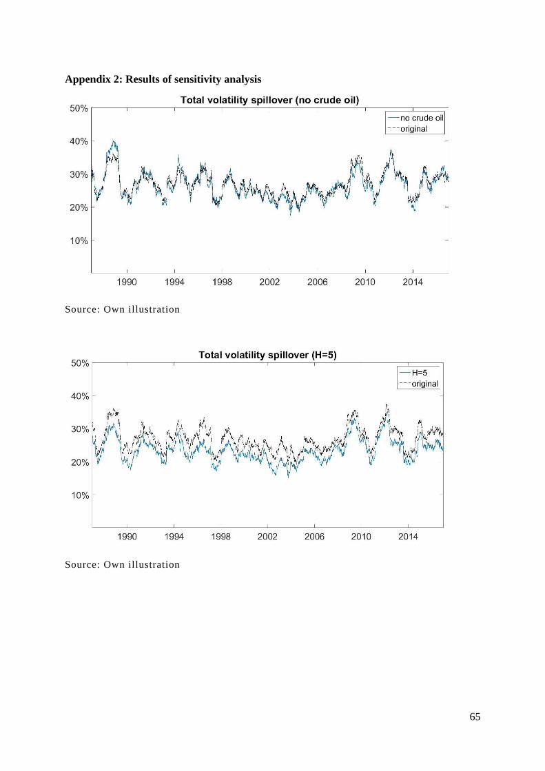
65
Appendix 2: Results of sensitivity analysis
Source: Own illustration
Source: Own illustration
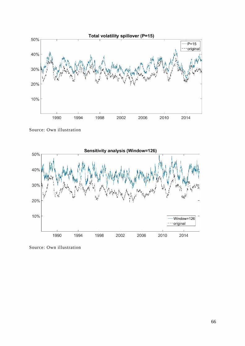
66
Source: Own illustration
Source: Own illustration
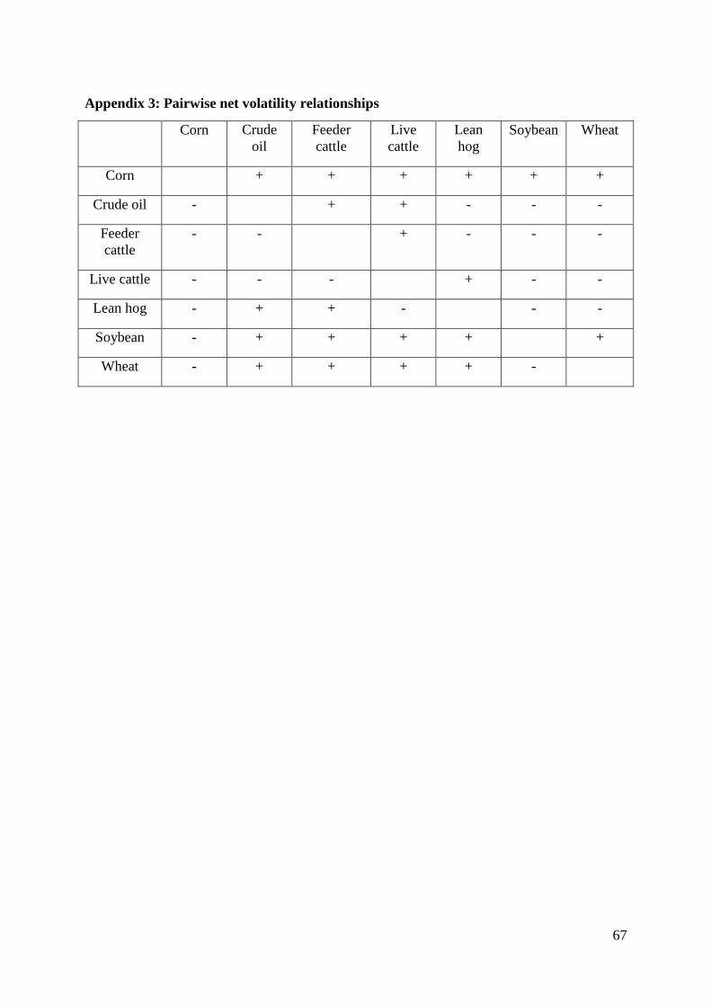
67
Appendix 3: Pairwise net volatility relationships
Corn Crude
oil
Feeder
cattle
Live
cattle
Lean
hog
Soybean Wheat
Corn + + + + + +
Crude oil - + + - - -
Feeder
cattle
- - + - - -
Live cattle - - - + - -
Lean hog - + + - - -
Soybean - + + + + +
Wheat - + + + + -
68
Declaration
I hereby affirm that I have prepared the present paper self-dependently, and without the use of
any other tools, than the ones indicated. All parts of the text, having been taken over verbatim
or analogously from published or not published scripts, are indicated as such. The thesis
hasn’t yet been submitted in the same or similar form, or in extracts within the context of an-
other examination.
Hennef, 30.05.2017
_______________________________
Student’s signature