Embed Size (px)
DESCRIPTION
ZondGM2D gravity and magnetic interpretation softwareenglish manual
Citation preview

Zond geophysical software Saint-Petersburg 2001-2013
1
PROGRAM FOR 2D INTERPRETATION
OF MAGNETIC AND GRAVITY DATA
ZONDGM2D
PROGRAM FUNCTIONALITY __________________________________________________ 2
SYSTEM REQUIREMENTS ____________________________________________________ 4
PROGRAM INSTALLATION AND DEINSTALLATION _____________________________ 4
PROGRAM REGISTRATION ___________________________________________________ 5
DENSITY OF THE ROCKS _____________________________________________________ 5
MAGNETIC SUSCEPTIBILITY OF ROCKS AND ORES ____________________________ 6
DESCRIPTION OF THE PROGRAM FUNCTIONAL _______________________________ 8
The toolbar of the main window ______________________________________________________ 8
Functions of the main window menu __________________________________________________ 9
“Hot” keys _______________________________________________________________________ 14
Status panel ______________________________________________________________________ 14
WORKING GUIDELINES _____________________________________________________ 15
Preparing and opening a data file ____________________________________________________ 15
Import and export data ____________________________________________________________ 16
Saving of interpretation results ______________________________________________________ 21
Getting start with the program ______________________________________________________ 22
Dialog of program parameters settings _______________________________________________ 25
Profiling plots (Profile) _____________________________________________________________ 32
Model editor _____________________________________________________________________ 33 Working with a model ____________________________________________________________________ 37 Dialog of model settings __________________________________________________________________ 38 Cell parameters setup dialog _______________________________________________________________ 39
Selection of medium model in inversion (modes of regular cells grid, polygonal and randomly
layered medium) __________________________________________________________________ 40
MODELING ________________________________________________________________ 43
Modes of polygonal modeling and modeling using arbitrary layered medium _______________ 45
ADVANCED PROGRAM OPTIONS _____________________________________________ 50
Euler deconvolution _______________________________________________________________ 50
Downward continuation ____________________________________________________________ 52
Cell summarization dialog __________________________________________________________ 52
Option «Buffer» of the main menu ___________________________________________________ 53
Zond geophysical software Saint-Petersburg 2001-2013
2
Geological sections editor ___________________________________________________________ 54
Working with areal data and 3D visualization _________________________________________ 59
A priori information input __________________________________________________________ 64
ADJUSTING PROGRAM INTERFACE __________________________________________ 68
Palette settings____________________________________________________________________ 68
Axes editor _______________________________________________________________________ 69
Graph’s editor ____________________________________________________________________ 73
Print preview dialog _______________________________________________________________ 75
PROGRAM DATA FILE FORMAT _____________________________________________ 76
Data file format ___________________________________________________________________ 76
Logging and lithology data file format ________________________________________________ 77
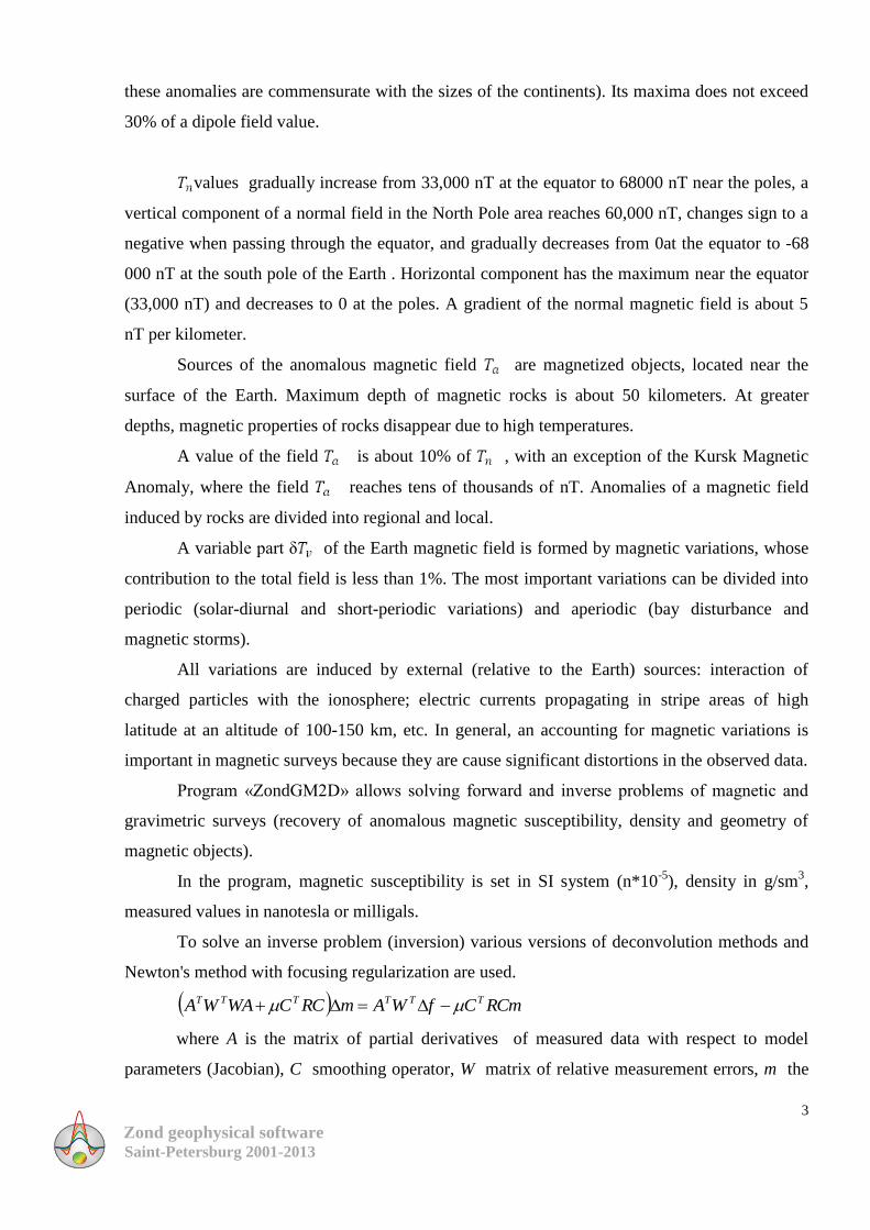
PROGRAM FUNCTIONALITY
«ZondGM2D» is a computer program for 2D interpretation of profile and areal multi-
level data obtained from magnetic and gravity surveys. User-friendly interface and rich options
for data presentation allows solving existing geological problems with maximum efficiency.
The traditional exploration method for iron-bearing formations is magnetic survey. It
studies magnetic fields of objects, which contain ferromagnetic minerals. Physical interrelation
between data measured at the surface and magnetic properties at depths allows assuming
presence of magnetic bodies.
In magnetic exploration, total magnetic field is measured. It is comprised of the Earth
normal field, anomalous fields caused by magnetized bodies and magnetic field variations,
mostly related to the solar activity. A useful component associated with a studying area is
anomalous field, which can be identified, taking into account the normal field and measuring
magnetic variations in the vicinity of a survey area.
The magnetic field on the Earth surface can be represented as a vector sum:
, where and are normal and anomalous magnetic fields, magnetic
field variations. The normal field is divided into a dipole ( ) and non-dipole ( )
components, that is .
The dipole field , which, to a first-order approximation, is the magnetic field of the
Earth, is a field of a homogeneous magnetized sphere. The difference between the dipole field
(calculated) and areal and normal field (measured by satellite) is a non-dipole part of the
normal field. It is often named as a residual field or a field of continental anomalies (sizes of
Zond geophysical software Saint-Petersburg 2001-2013
3
these anomalies are commensurate with the sizes of the continents). Its maxima does not exceed
30% of a dipole field value.
values gradually increase from 33,000 nT at the equator to 68000 nT near the poles, a
vertical component of a normal field in the North Pole area reaches 60,000 nT, changes sign to a
negative when passing through the equator, and gradually decreases from 0at the equator to -68
000 nT at the south pole of the Earth . Horizontal component has the maximum near the equator
(33,000 nT) and decreases to 0 at the poles. A gradient of the normal magnetic field is about 5
nT per kilometer.
Sources of the anomalous magnetic field are magnetized objects, located near the
surface of the Earth. Maximum depth of magnetic rocks is about 50 kilometers. At greater
depths, magnetic properties of rocks disappear due to high temperatures.
A value of the field is about 10% of , with an exception of the Kursk Magnetic
Anomaly, where the field reaches tens of thousands of nT. Anomalies of a magnetic field
induced by rocks are divided into regional and local.
A variable part δ of the Earth magnetic field is formed by magnetic variations, whose
contribution to the total field is less than 1%. The most important variations can be divided into
periodic (solar-diurnal and short-periodic variations) and aperiodic (bay disturbance and
magnetic storms).
All variations are induced by external (relative to the Earth) sources: interaction of
charged particles with the ionosphere; electric currents propagating in stripe areas of high
latitude at an altitude of 100-150 km, etc. In general, an accounting for magnetic variations is
important in magnetic surveys because they are cause significant distortions in the observed data.
Program «ZondGM2D» allows solving forward and inverse problems of magnetic and
gravimetric surveys (recovery of anomalous magnetic susceptibility, density and geometry of
magnetic objects).
In the program, magnetic susceptibility is set in SI system (n*10-5
), density in g/sm3,
measured values in nanotesla or milligals.
To solve an inverse problem (inversion) various versions of deconvolution methods and
Newton's method with focusing regularization are used.
RCmCfWAmRCCWAWA TTTTTT
where A is the matrix of partial derivatives of measured data with respect to model
parameters (Jacobian), C smoothing operator, W matrix of relative measurement errors, m the

Zond geophysical software Saint-Petersburg 2001-2013
4
model parameter vector, μ - regularizing parameter, Δf vector of residuals between the observed
and calculated values, R focusing operator.
During the development of inverse problem, special attention was given to a priori
information usage (weights of individual measurements, ranges of parameters).
«ZondGM2D» uses a simple and clear data file format.
Program allows importing and visualizing data using other methods which makes data
interpretation process more integrated.
«ZondGM2D» is an easy-to-use instrument for automatic and interactive multilevel data
interpretation of magnetic and gravity surveys, and can be used on IBM-PC compatible PCs with
Windows operating system.
SYSTEM REQUIREMENTS
«ZondGM2D» can be installed on a PC with OS Windows 98 and higher. Recommended
system parameters are processor P IV-2 GHz, memory 512 Mb, screen resolution 1024 X 768,
color mode – True color (screen resolution change is not recommended while working with
data).
As far as the program is actively using the registry, it is recommended to launch it as
administrator (right click on program shortcut – run as administrator), when using higher than
Windows XP systems.
PROGRAM INSTALLATION AND DEINSTALLATION
«ZondGM2D» program is supplied on CD or by internet. Current manual is included in
the delivery set. Latest updates of the program can be downloaded from website: www.zond-
geo.ru.
To install the program copy it from CD to necessary directory (e.g., Zond). To install
updates rewrite previous version of the program with the new one.
Secure key SenseLock driver must be installed before starting the program. To do that
open SenseLock folder (the driver can be downloaded from CD or website) and run
InstWiz3.exe file. After installation of the driver insert key. If everything is all right, a message
announcing that the key is detected will appear in the lower system panel.
To uninstall the program delete work directory of the program.
Zond geophysical software Saint-Petersburg 2001-2013
5
PROGRAM REGISTRATION
For registration click “Registration file” item of the main menu of the program. When a dialog
appears, select registration file name, and save it. Created file is transmitted to specified in the
contract address. After that user receives unique password which depends on HDD serial
number. Input this password in “Registration” field. The second option is to use the program
with supplied SenseLock key inserted in a USB-port while working.
DENSITY OF THE ROCKS
It is essential to know rock density σ which is the only physical parameter that gravity
survey is based on to perform gravity surveying and especially to interpret results.
Rock density (or volume weight) is defined as its mass per unit volume. Density unit is
g/sm3. Density is usually measured on samples taken from natural outcrop, boreholes or mines.
The easiest way to measure density is to weight the sample in the air and in water and then
calculate density σ. The most popular and handy device for density measurement is densitometer
and it is based on this principle. Densitometer defines density within the accuracy of 0,01 g/sm3
[Hmelevskoj, 1997].
In order to receive reliable and representative data it is necessary to measure large
quantity of samples (up to 50). On the basis of numerous density measurements on samples
from the same lithological sequence variation curve or cross-plot of σ values versus number of
samples characterized by current density is constructed. Curve maximum corresponds to the
most probable density value for current rock. There are gravimetric and other geophysical
methods of field and borehole density assessment.
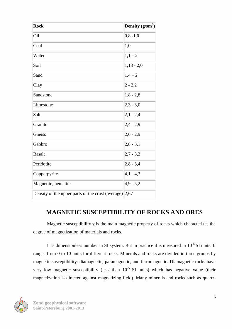
Density of rocks and ores depends on chemical-mineral composition, in other words on
bulk density of solid particles, porosity, and pore filler composition (water, solutions, oil, gas).
Density of volcanic and metamorphic rocks is mostly defined bytheir mineral composition and
increases in going from acidic to base and ultrabasic rocks. Density of sedimentary rocks first of
all depends on porosity, water saturation, and to lesser degree on mineral composition. But it
strongly depends on deposits consolidation, their age, and depth of burial (their increase leads to
density increase as well). Examples of density are given below [Hmelevskoj, 1997].
Zond geophysical software Saint-Petersburg 2001-2013
6
Rock Density (g/sm3)
Oil 0,8 -1,0
Coal 1,0
Water 1,1 – 2
Soil 1,13 - 2,0
Sand 1,4 – 2
Clay 2 - 2,2
Sandstone 1,8 - 2,8
Limestone 2,3 - 3,0
Salt 2,1 - 2,4
Granite 2,4 - 2,9
Gneiss 2,6 - 2,9
Gabbro 2,8 - 3,1
Basalt 2,7 - 3,3
Peridotite 2,8 - 3,4
Copperpyrite 4,1 - 4,3
Magnetite, hematite 4,9 - 5,2
Density of the upper parts of the crust (average) 2,67
MAGNETIC SUSCEPTIBILITY OF ROCKS AND ORES
Magnetic susceptibility χ is the main magnetic property of rocks which characterizes the
degree of magnetization of materials and rocks.
It is dimensionless number in SI system. But in practice it is measured in 10-5
SI units. It
ranges from 0 to 10 units for different rocks. Minerals and rocks are divided in three groups by
magnetic susceptibility: diamagnetic, paramagnetic, and ferromagnetic. Diamagnetic rocks have
very low magnetic susceptibility (less than 10-5
SI units) which has negative value (their
magnetization is directed against magnetizing field). Many minerals and rocks such as quartz,
Zond geophysical software Saint-Petersburg 2001-2013
7
mine salt, marble, oil, ice, graphite, gold, silver, lead, copper, etc. are diamagnetic [Hmelevskoj,
1997].
Paramagnetic rocks have positive magnetic susceptibility with low values. The majority
of minerals, sedimentary, metamorphic, and volcanic rocks are paramagnetic.
Ferromagnetic minerals (e.g. magnetite, titaniferous magnetite, ilmenite, pyrrhotite) have
very large χ values (up to several millions of 10-5
SI units).
Magnetic susceptibility of the majority of rocks depends largely on the presence and
percentage of ferromagnetic minerals in their composition.
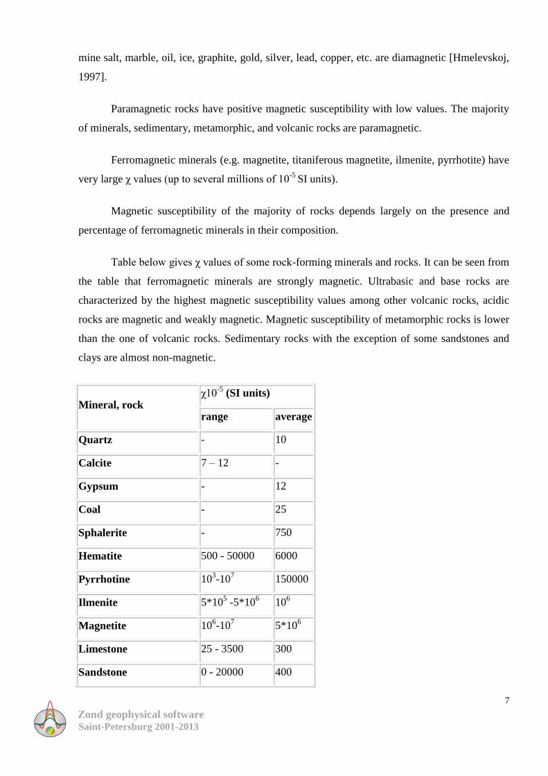
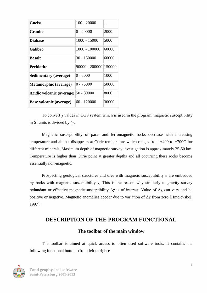
Table below gives χ values of some rock-forming minerals and rocks. It can be seen from
the table that ferromagnetic minerals are strongly magnetic. Ultrabasic and base rocks are
characterized by the highest magnetic susceptibility values among other volcanic rocks, acidic
rocks are magnetic and weakly magnetic. Magnetic susceptibility of metamorphic rocks is lower
than the one of volcanic rocks. Sedimentary rocks with the exception of some sandstones and
clays are almost non-magnetic.
Mineral, rock χ10
-5 (SI units)
range average
Quartz - 10
Calcite 7 – 12 -
Gypsum - 12
Coal - 25
Sphalerite - 750
Hematite 500 - 50000 6000
Pyrrhotine 103-10
7 150000
Ilmenite 5*105 -5*10
6 10
6
Magnetite 106-10
7 5*10
6
Limestone 25 - 3500 300
Sandstone 0 - 20000 400
Zond geophysical software Saint-Petersburg 2001-2013
8
Gneiss 100 - 20000 -
Granite 0 - 40000 2000
Diabase 1000 - 15000 5000
Gabbro 1000 - 100000 60000
Basalt 30 - 150000 60000
Peridotite 90000 - 200000 150000
Sedimentary (average) 0 - 5000 1000
Metamorphic (average) 0 - 75000 50000
Acidic volcanic (average) 50 - 80000 8000
Base volcanic (average) 60 - 120000 30000
To convert χ values in CGS system which is used in the program, magnetic susceptibility
in SI units is divided by 4π.
Magnetic susceptibility of para- and ferromagnetic rocks decrease with increasing
temperature and almost disappears at Curie temperature which ranges from +400 to +700C for
different minerals. Maximum depth of magnetic survey investigation is approximately 25-50 km.
Temperature is higher than Curie point at greater depths and all occurring there rocks become
essentially non-magnetic.
Prospecting geological structures and ores with magnetic susceptibility are embedded
by rocks with magnetic susceptibility χ. This is the reason why similarly to gravity survey
redundant or effective magnetic susceptibility Δχ is of interest. Value of Δχ can vary and be
positive or negative. Magnetic anomalies appear due to variation of Δχ from zero [Hmelevskoj,
1997].
DESCRIPTION OF THE PROGRAM FUNCTIONAL
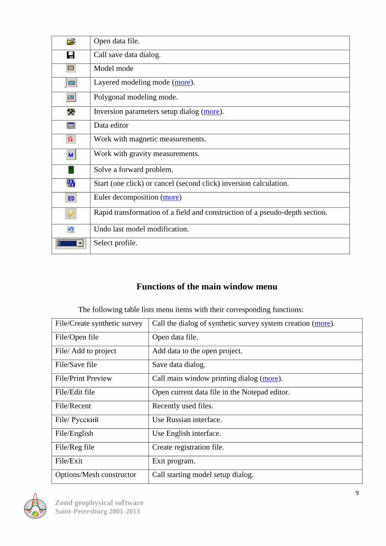
The toolbar of the main window
The toolbar is aimed at quick access to often used software tools. It contains the
following functional buttons (from left to right):
Zond geophysical software Saint-Petersburg 2001-2013
9
Open data file.
Call save data dialog.
Model mode
Layered modeling mode (more).
Polygonal modeling mode.
Inversion parameters setup dialog (more).
Data editor
Work with magnetic measurements.
Work with gravity measurements.
Solve a forward problem.
Start (one click) or cancel (second click) inversion calculation.
Euler decomposition (more)
Rapid transformation of a field and construction of a pseudo-depth section.
Undo last model modification.
Select profile.
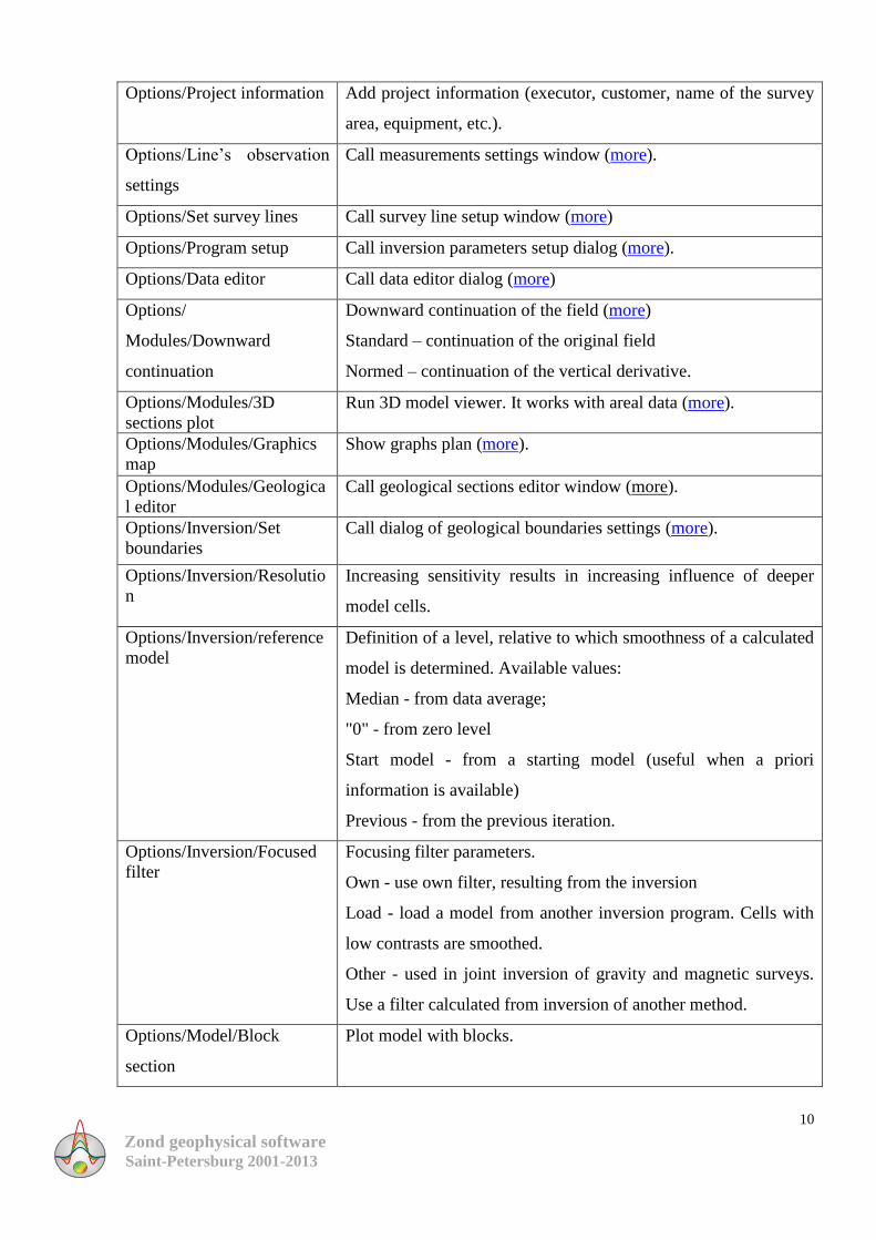
Functions of the main window menu
The following table lists menu items with their corresponding functions:
File/Create synthetic survey Call the dialog of synthetic survey system creation (more).
File/Open file Open data file.
File/ Add to project Add data to the open project.
File/Save file Save data dialog.
File/Print Preview Call main window printing dialog (more).
File/Edit file Open current data file in the Notepad editor.
File/Recent Recently used files.
File/ Русский Use Russian interface.
File/English Use English interface.
File/Reg file Create registration file.
File/Exit Exit program.
Options/Mesh constructor Call starting model setup dialog.
Zond geophysical software Saint-Petersburg 2001-2013
10
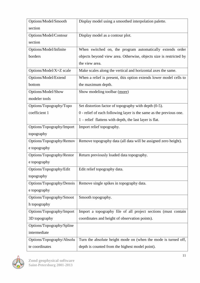
Options/Project information Add project information (executor, customer, name of the survey
area, equipment, etc.).
Options/Line’s observation
settings
Call measurements settings window (more).
Options/Set survey lines Call survey line setup window (more)
Options/Program setup Call inversion parameters setup dialog (more).
Options/Data editor Call data editor dialog (more)
Options/
Modules/Downward
continuation
Downward continuation of the field (more)
Standard – continuation of the original field
Normed – continuation of the vertical derivative.
Options/Modules/3D
sections plot
Run 3D model viewer. It works with areal data (more).
Options/Modules/Graphics
map
Show graphs plan (more).
Options/Modules/Geologica
l editor
Call geological sections editor window (more).
Options/Inversion/Set
boundaries
Call dialog of geological boundaries settings (more).
Options/Inversion/Resolutio
n
Increasing sensitivity results in increasing influence of deeper
model cells.
Options/Inversion/reference
model
Definition of a level, relative to which smoothness of a calculated
model is determined. Available values:
Median - from data average;
"0" - from zero level
Start model - from a starting model (useful when a priori
information is available)
Previous - from the previous iteration.
Options/Inversion/Focused
filter
Focusing filter parameters.
Own - use own filter, resulting from the inversion
Load - load a model from another inversion program. Cells with
low contrasts are smoothed.
Other - used in joint inversion of gravity and magnetic surveys.
Use a filter calculated from inversion of another method.
Options/Model/Block
section
Plot model with blocks.
Zond geophysical software Saint-Petersburg 2001-2013
11
Options/Model/Smooth
section
Display model using a smoothed interpolation palette.
Options/Model/Contour
section
Display model as a contour plot.
Options/Model/Infinite
borders
When switched on, the program automatically extends order
objects beyond view area. Otherwise, objects size is restricted by
the view area.
Options/Model/X=Z scale Make scales along the vertical and horizontal axes the same.
Options/Model/Extend
bottom
When a relief is present, this option extends lower model cells to
the maximum depth.
Options/Model/Show
modeler tools
Show modeling toolbar (more)
Options/Topography/Topo
coefficient 1
Set distortion factor of topography with depth (0-5).
0 - relief of each following layer is the same as the previous one.
1 – relief flattens with depth, the last layer is flat.
Options/Topography/Import
topography
Import relief topography.
Options/Topography/Remov
e topography
Remove topography data (all data will be assigned zero height).
Options/Topography/Restor
e topography
Return previously loaded data topography.
Options/Topography/Edit
topography
Edit relief topography data.
Options/Topography/Denois
e topography
Remove single spikes in topography data.
Options/Topography/Smoot
h topography
Smooth topography.
Options/Topography/Import
3D topography
Import a topography file of all project sections (must contain
coordinates and height of observation points).
Options/Topography/Spline
intermediate
Options/Topography/Absolu
te coordinates
Turn the absolute height mode on (when the mode is turned off,
depth is counted from the highest model point).
Zond geophysical software Saint-Petersburg 2001-2013
12
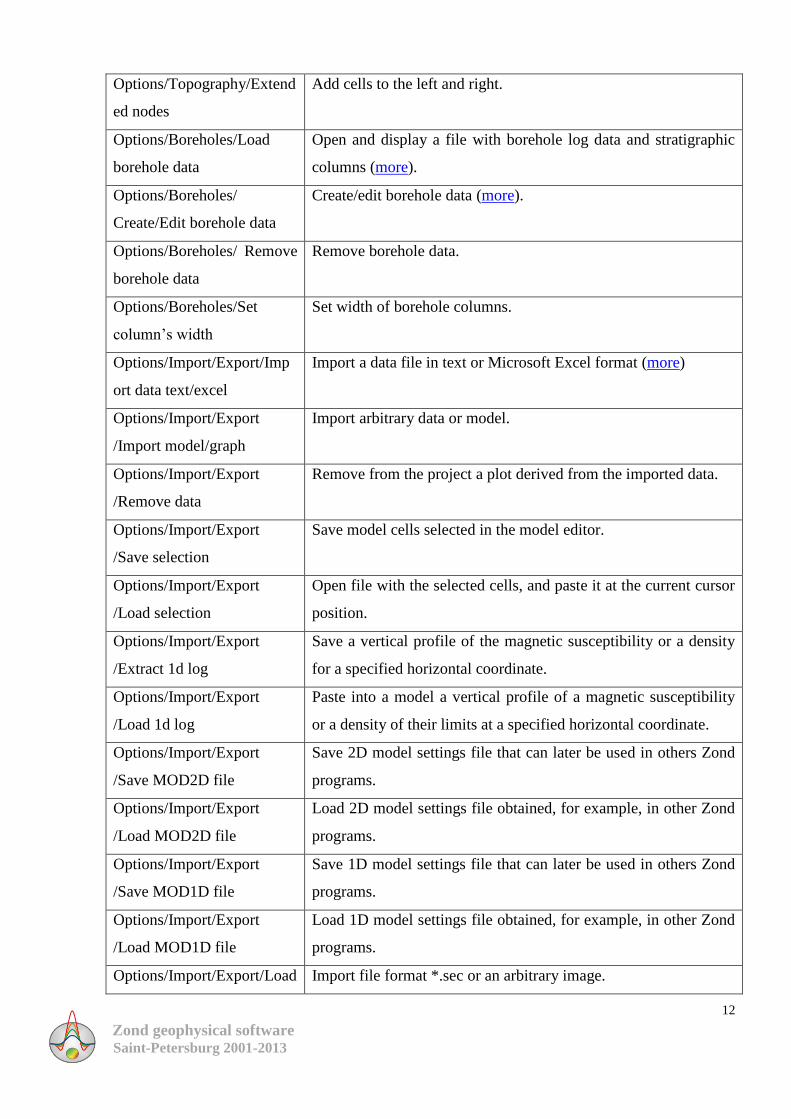
Options/Topography/Extend
ed nodes
Add cells to the left and right.
Options/Boreholes/Load
borehole data
Open and display a file with borehole log data and stratigraphic
columns (more).
Options/Boreholes/
Create/Edit borehole data
Create/edit borehole data (more).
Options/Boreholes/ Remove
borehole data
Remove borehole data.
Options/Boreholes/Set
column’s width
Set width of borehole columns.
Options/Import/Export/Imp
ort data text/excel
Import a data file in text or Microsoft Excel format (more)
Options/Import/Export
/Import model/graph
Import arbitrary data or model.
Options/Import/Export
/Remove data
Remove from the project a plot derived from the imported data.
Options/Import/Export
/Save selection
Save model cells selected in the model editor.
Options/Import/Export
/Load selection
Open file with the selected cells, and paste it at the current cursor
position.
Options/Import/Export
/Extract 1d log
Save a vertical profile of the magnetic susceptibility or a density
for a specified horizontal coordinate.
Options/Import/Export
/Load 1d log
Paste into a model a vertical profile of a magnetic susceptibility
or a density of their limits at a specified horizontal coordinate.
Options/Import/Export
/Save MOD2D file
Save 2D model settings file that can later be used in others Zond
programs.
Options/Import/Export
/Load MOD2D file
Load 2D model settings file obtained, for example, in other Zond
programs.
Options/Import/Export
/Save MOD1D file
Save 1D model settings file that can later be used in others Zond
programs.
Options/Import/Export
/Load MOD1D file
Load 1D model settings file obtained, for example, in other Zond
programs.
Options/Import/Export/Load Import file format *.sec or an arbitrary image.
Zond geophysical software Saint-Petersburg 2001-2013
13
background image
Options/Import/Export/Rem
ove background image
Remove background image.
Options/Import/Export/Sho
w background image
Show exporting image.
Options/Import/Export/Resi
ze background image
Resize exporting image.
Options/Import/Export/Exp
ort to Excel
Save model in Excel format.
Options/Import/Export/Exp
ort model to DXF
Save model in AutoCAD format (*.DXF)
Options/Import/Export/Dra
w model in Surfer
Export model to Surfer.
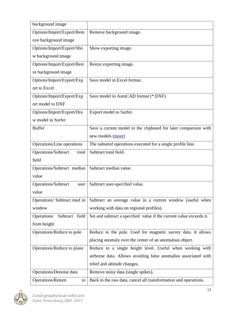
Buffer Save a current model to the clipboard for later comparison with
new models (more)
Operations/Line operations The subsetof operations executed for a single profile line.
Operations/Subtract total
field
Subtract total field.
Operations/Subtract median
value
Subtract median value.
Operations/Subtract user
value
Subtract user-specified value.
Operations/ Subtract med in
window
Subtract an average value in a current window (useful when
working with data on regional profiles).
Operations/ Subtract field
from height
Set and subtract a specified value if the current value exceeds it.
Operations/Reduce to pole Reduce to the pole. Used for magnetic survey data. It allows
placing anomaly over the center of an anomalous object.
Operations/Reduce to plane Reduce to a single height level. Useful when working with
airborne data. Allows avoiding false anomalies associated with
relief and altitude changes.
Operations/Denoise data Remove noisy data (single spikes).
Operations/Return to Back to the raw data, cancel all transformation and operations.
Zond geophysical software Saint-Petersburg 2001-2013
14
original
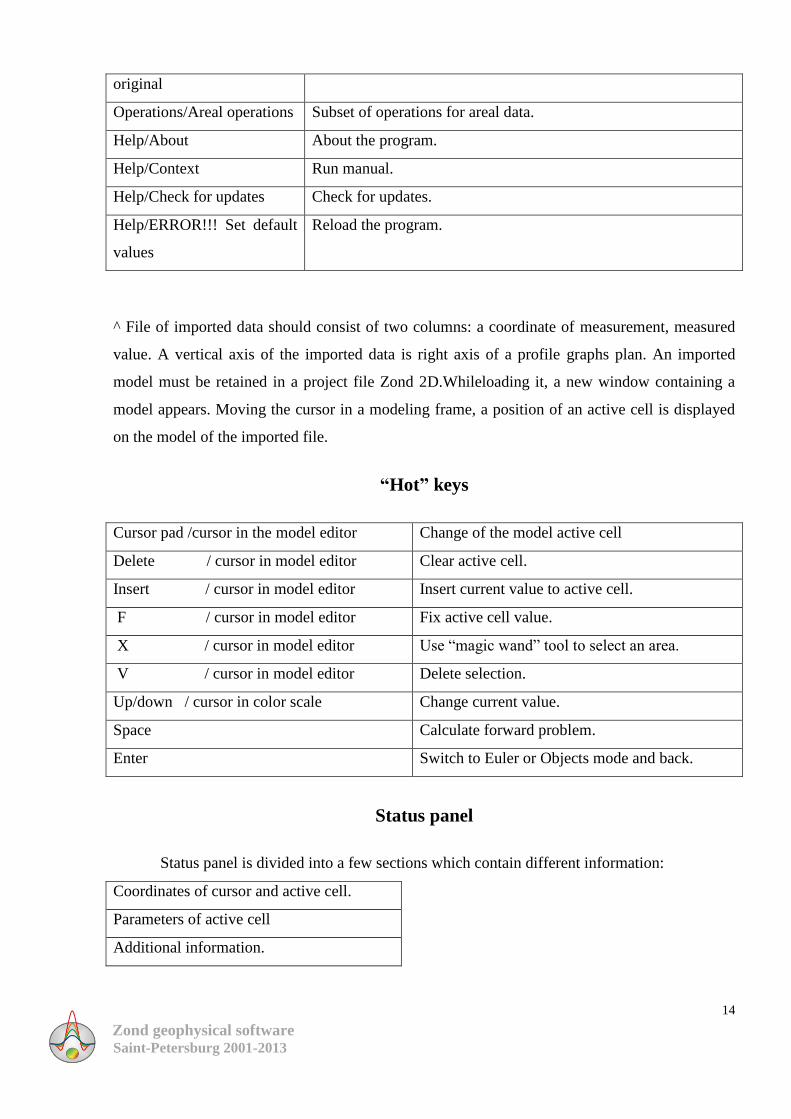
Operations/Areal operations Subset of operations for areal data.
Help/About About the program.
Help/Context Run manual.
Help/Check for updates Check for updates.
Help/ERROR!!! Set default
values
Reload the program.
^ File of imported data should consist of two columns: a coordinate of measurement, measured
value. A vertical axis of the imported data is right axis of a profile graphs plan. An imported
model must be retained in a project file Zond 2D.Whileloading it, a new window containing a
model appears. Moving the cursor in a modeling frame, a position of an active cell is displayed
on the model of the imported file.
“Hot” keys
Cursor pad /cursor in the model editor Change of the model active cell
Delete / cursor in model editor Clear active cell.
Insert / cursor in model editor Insert current value to active cell.
F / cursor in model editor Fix active cell value.
X / cursor in model editor Use “magic wand” tool to select an area.
V / cursor in model editor Delete selection.
Up/down / cursor in color scale Change current value.
Space Calculate forward problem.
Enter Switch to Euler or Objects mode and back.
Status panel
Status panel is divided into a few sections which contain different information:
Coordinates of cursor and active cell.
Parameters of active cell
Additional information.
Zond geophysical software Saint-Petersburg 2001-2013
15
WORKING GUIDELINES
Preparing and opening a data file
To begin working with « ZONDGM2D», it is necessary to have a data file of specific
format which contains information about measurement positions and measured values.
One file usually contains data obtained from one profile. Text data files created in
«ZONDGM2D» format have «*.GM» extension. See data file format section for more details.
For correct work of the program data file must not contain:
unconventional separation symbols (use TABs and SPACEs only);
invalid values of measured data
It is desirable to not have more than 5000 observed data values in a single file.
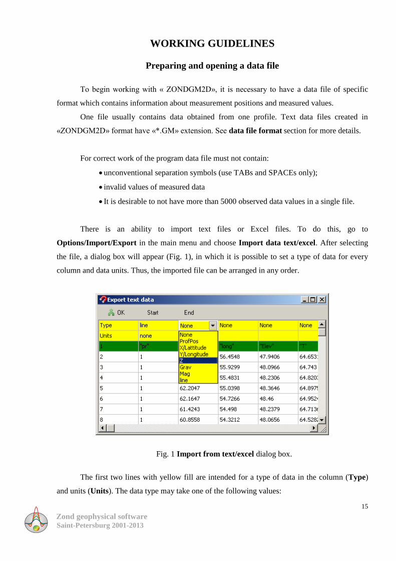
There is an ability to import text files or Excel files. To do this, go to
Options/Import/Export in the main menu and choose Import data text/excel. After selecting
the file, a dialog box will appear (Fig. 1), in which it is possible to set a type of data for every
column and data units. Thus, the imported file can be arranged in any order.
Fig. 1 Import from text/excel dialog box.
The first two lines with yellow fill are intended for a type of data in the column (Type)
and units (Units). The data type may take one of the following values:
Zond geophysical software Saint-Petersburg 2001-2013
16
ProfPos - number of a measurement point
X/Latitude - horizontal coordinate/latitude
Y/Longitude - vertical coordinate/longitude
Z – height
Grav - measured values of gravity field
Mag - measured values of magnetic field
line - a profile number
The first line of the opened file is displayed on the third line with a green filling color.
The keys Start and End on the panel dialog are intended to define the first and last
imported rows, respectively. After selection of all necessary parameters, click OK.
There is an ability to add data to the project, which is useful when working with areal
data.
Import and export data
The tab of the main menu Options/Import/Export contains program options for
importing data of different types (raw data, data from other methods in the form of underlying
image, etc.) and for exporting data to different software packages. These options allow a user to
compare data from different methods, to load data of gravity and magnetic surveys of any data
format, to plot quickly results obtained in other programs.
There is an ability to import text files or Excel files. To do this, choose the item Import
data from text/excel. After selecting the file, a dialog box will appear (Fig.2), in which it is
possible to set a type of data for every column and data units. Thus, the imported file can be
arranged in any order.
Zond geophysical software Saint-Petersburg 2001-2013
17
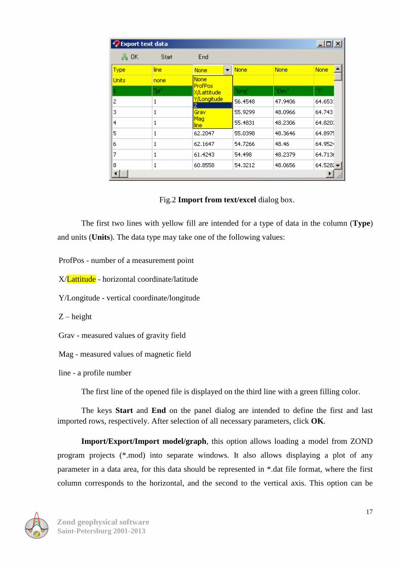
Fig.2 Import from text/excel dialog box.
The first two lines with yellow fill are intended for a type of data in the column (Type)
and units (Units). The data type may take one of the following values:
ProfPos - number of a measurement point
X/Lattitude - horizontal coordinate/latitude
Y/Longitude - vertical coordinate/longitude
Z – height
Grav - measured values of gravity field
Mag - measured values of magnetic field
line - a profile number
The first line of the opened file is displayed on the third line with a green filling color.
The keys Start and End on the panel dialog are intended to define the first and last
imported rows, respectively. After selection of all necessary parameters, click OK.
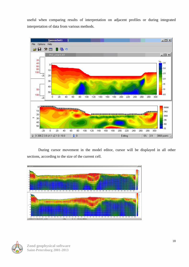
Import/Export/Import model/graph, this option allows loading a model from ZOND
program projects (*.mod) into separate windows. It also allows displaying a plot of any
parameter in a data area, for this data should be represented in *.dat file format, where the first
column corresponds to the horizontal, and the second to the vertical axis. This option can be
Zond geophysical software Saint-Petersburg 2001-2013
18
useful when comparing results of interpretation on adjacent profiles or during integrated
interpretation of data from various methods.
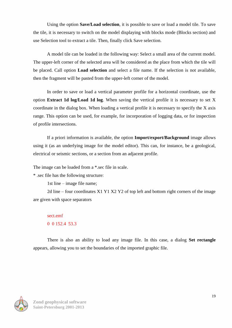
During cursor movement in the model editor, cursor will be displayed in all other
sections, according to the size of the current cell.
Zond geophysical software Saint-Petersburg 2001-2013
19
Using the option Save/Load selection, it is possible to save or load a model tile. To save
the tile, it is necessary to switch on the model displaying with blocks mode (Blocks section) and
use Selection tool to extract a tile. Then, finally click Save selection.
A model tile can be loaded in the following way: Select a small area of the current model.
The upper-left corner of the selected area will be considered as the place from which the tile will
be placed. Call option Load selection and select a file name. If the selection is not available,
then the fragment will be pasted from the upper-left corner of the model.
In order to save or load a vertical parameter profile for a horizontal coordinate, use the
option Extract 1d log/Load 1d log. When saving the vertical profile it is necessary to set X
coordinate in the dialog box. When loading a vertical profile it is necessary to specify the X axis
range. This option can be used, for example, for incorporation of logging data, or for inspection
of profile intersections.
If a priori information is available, the option Import/export/Background image allows
using it (as an underlying image for the model editor). This can, for instance, be a geological,
electrical or seismic sections, or a section from an adjacent profile.
The image can be loaded from a *.sec file in scale.
* .sec file has the following structure:
1st line – image file name;
2d line – four coordinates X1 Y1 X2 Y2 of top left and bottom right corners of the image
are given with space separators
sect.emf
0 0 152.4 53.3
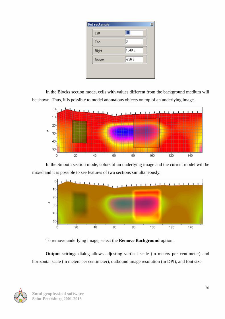
There is also an ability to load any image file. In this case, a dialog Set rectangle
appears, allowing you to set the boundaries of the imported graphic file.
Zond geophysical software Saint-Petersburg 2001-2013
20
In the Blocks section mode, cells with values different from the background medium will
be shown. Thus, it is possible to model anomalous objects on top of an underlying image.
In the Smooth section mode, colors of an underlying image and the current model will be
mixed and it is possible to see features of two sections simultaneously.
To remove underlying image, select the Remove Background option.
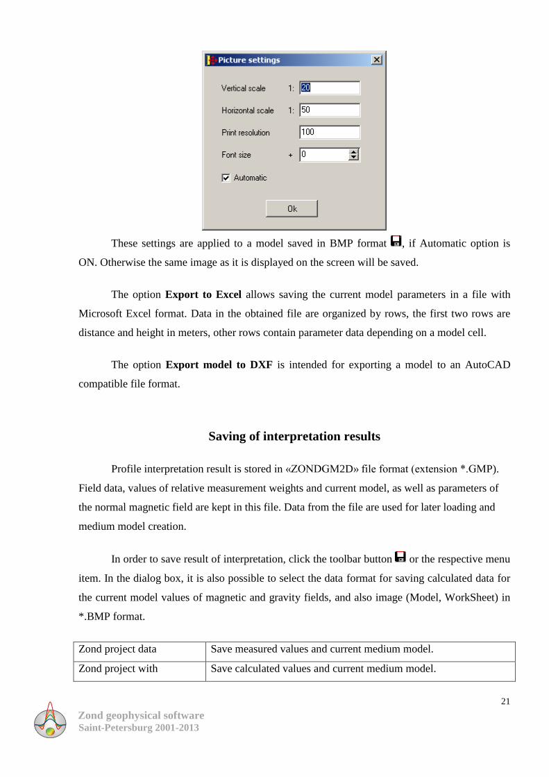
Output settings dialog allows adjusting vertical scale (in meters per centimeter) and
horizontal scale (in meters per centimeter), outbound image resolution (in DPI), and font size.
Zond geophysical software Saint-Petersburg 2001-2013
21
These settings are applied to a model saved in BMP format , if Automatic option is
ON. Otherwise the same image as it is displayed on the screen will be saved.
The option Export to Excel allows saving the current model parameters in a file with
Microsoft Excel format. Data in the obtained file are organized by rows, the first two rows are
distance and height in meters, other rows contain parameter data depending on a model cell.
The option Export model to DXF is intended for exporting a model to an AutoCAD
compatible file format.
Saving of interpretation results
Profile interpretation result is stored in «ZONDGM2D» file format (extension *.GMP).
Field data, values of relative measurement weights and current model, as well as parameters of
the normal magnetic field are kept in this file. Data from the file are used for later loading and
medium model creation.
In order to save result of interpretation, click the toolbar button or the respective menu
item. In the dialog box, it is also possible to select the data format for saving calculated data for
the current model values of magnetic and gravity fields, and also image (Model, WorkSheet) in
*.BMP format.
Zond project data Save measured values and current medium model.
Zond project with Save calculated values and current medium model.
Zond geophysical software Saint-Petersburg 2001-2013
22
calculated data
Worksheet Save three graphic window parts in BMP format.
Model Save bottom graphic part of the window in BMP format.
Grid file Save the current model as a grid file.
Section file Save the current model in *.sec format.
Save data as text Save measured, calculated data and additional information in text
format.
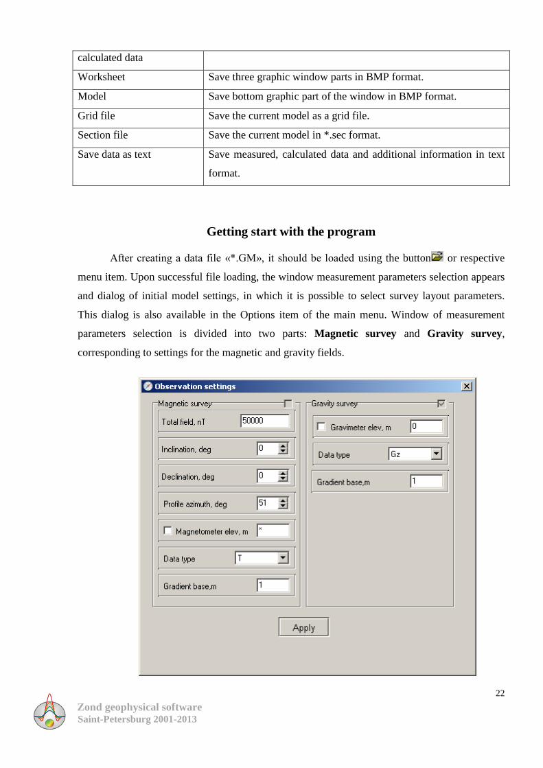
Getting start with the program
After creating a data file «*.GM», it should be loaded using the button or respective
menu item. Upon successful file loading, the window measurement parameters selection appears
and dialog of initial model settings, in which it is possible to select survey layout parameters.
This dialog is also available in the Options item of the main menu. Window of measurement
parameters selection is divided into two parts: Magnetic survey and Gravity survey,
corresponding to settings for the magnetic and gravity fields.
Zond geophysical software Saint-Petersburg 2001-2013
23
Magnetic survey part:
Total field, nT – magnitude of the normal magnetic field vector (T0), in nT.
Inclination, deg – a value of the normal magnetic field inclination, in degrees (I0). It is
counted down from horizontal.
Declination, deg – a value of the normal magnetic field declination, in degrees (D0). It is
counted clockwise from north.
Profile azimuth, deg – profile azimuth, in degrees. It is counted clockwise from north
Magnetometer elev, m –a height of a magneto active sensor, in meters, relative to relief.
Data type –a type of measured data. T is the magnetic field, GrZ - magnetic field gradient
Gradient base, m –a height of a sensor above the earth's surface
Gravity survey part:
Gravimeter elev, m – a gravimetric observations height, in meters, relative to the relief.
Data type – a type of measured data. Gz – vertical component of gravity force, Grz gradient
of Gz.
Gradient base, m – a sensor height above the earth's surface.
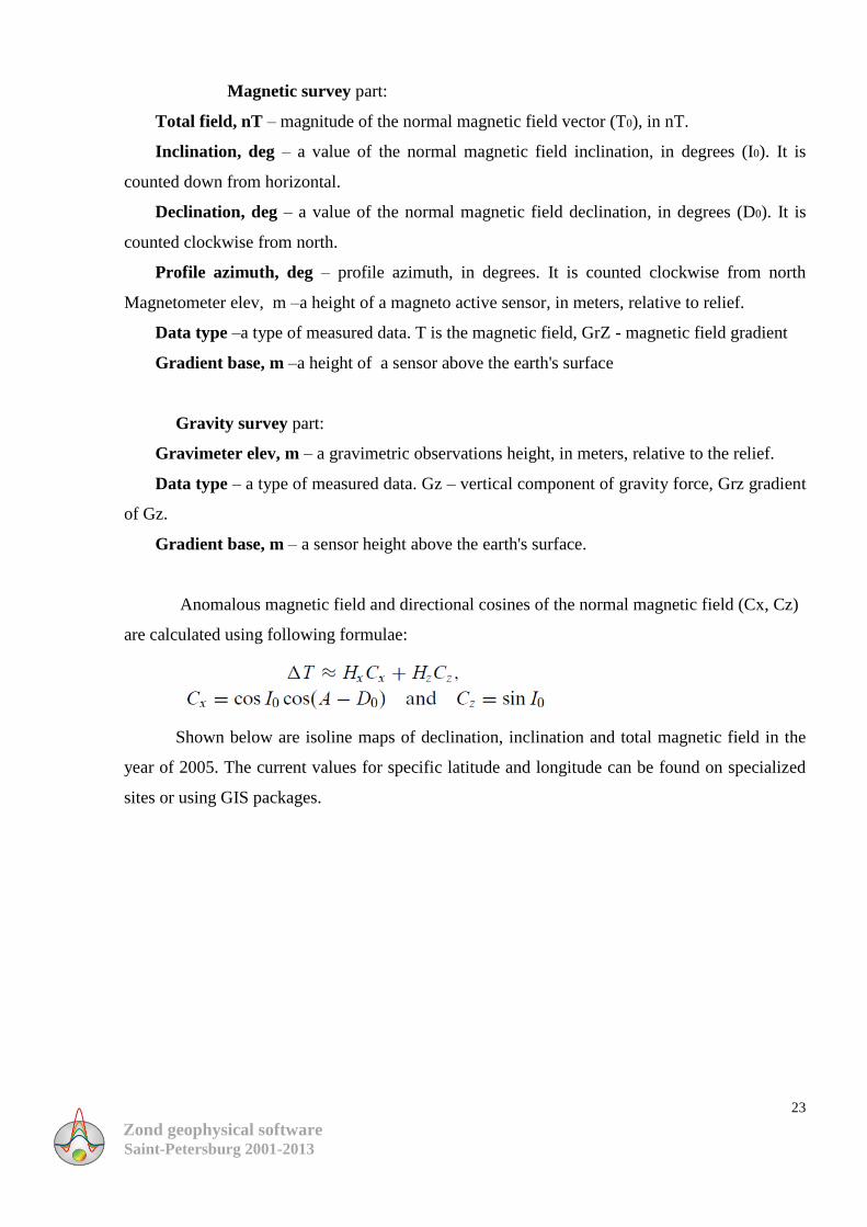
Anomalous magnetic field and directional cosines of the normal magnetic field (Cx, Cz)
are calculated using following formulae:
Shown below are isoline maps of declination, inclination and total magnetic field in the
year of 2005. The current values for specific latitude and longitude can be found on specialized
sites or using GIS packages.

Zond geophysical software Saint-Petersburg 2001-2013
24
Dialog of initial model settings Mesh constructor contains following options.
Area X nodes contains options, which allow setting the horizontal model grid parameters.
Minimum – set the minimum coordinate of the modelling area.
Maximum – set the maximum coordinate of modelling area.
Nodes number – if the option In points is OFF, it sets a number of uniformly distant
nodes of the horizontal grid; otherwise nodes are set at measurement points.
Zond geophysical software Saint-Petersburg 2001-2013
25
Regular mesh –set a uniform partition of a grid between measurement points (if the
option in points is ON).
Area Z nodes includes options, which allow setting parameters of a model vertical grid
(active for the borehole measurements).
StartH – set the first layer thickness. This value need to meet the required resolution.
Factor – set a ratio between the adjacent layers thicknesses. Values of the parameter are
generally selected in the range from 1 to 2.
Nodes number – sets a number of layers.
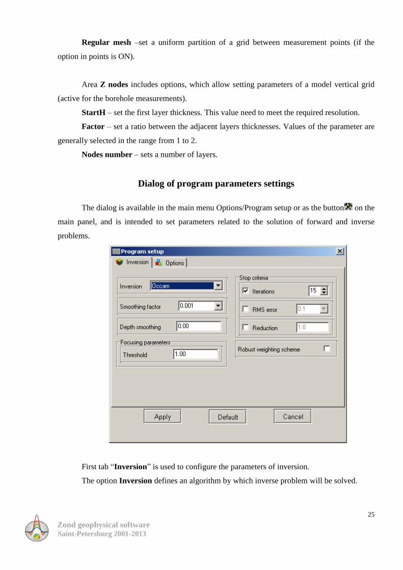
Dialog of program parameters settings
The dialog is available in the main menu Options/Program setup or as the button on the
main panel, and is intended to set parameters related to the solution of forward and inverse
problems.
First tab “Inversion” is used to configure the parameters of inversion.
The option Inversion defines an algorithm by which inverse problem will be solved.

Zond geophysical software Saint-Petersburg 2001-2013
26
Consider various inversion algorithms, as an example take a model consisting of several
blocks.
Consider various inversion algorithms, as an example take a model consisting of several
blocks.
To test algorithms calculate a theoretical response for the model and add a five per cent
Gaussian noise.
Smoothness constrained - inversion obtained by the least squares method using a
smoothing operator. As a result of using this algorithm, a smooth (without sharp boundaries) and
a stable distribution of the parameters are obtained.
The matrix equation for this inversion algorithm looks as follow:
fWAmCCWAWA TTTTT
As seen from the equation, inversion model contrast is not minimized. This algorithm
allows reaching minimum misfit values. It is recommended to use it in the initial interpretation,
in most cases.
Occam - inversion by least squares method with using a smoothing operator and
additional contrast minimization [Constable, 1987]. As a result of using this algorithm, we get
the more smooth parameters distribution.
Zond geophysical software Saint-Petersburg 2001-2013
27
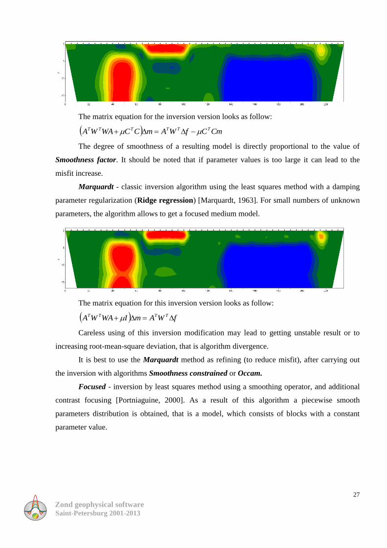
The matrix equation for the inversion version looks as follow:
CmCfWAmCCWAWA TTTTTT
The degree of smoothness of a resulting model is directly proportional to the value of
Smoothness factor. It should be noted that if parameter values is too large it can lead to the
misfit increase.
Marquardt - classic inversion algorithm using the least squares method with a damping
parameter regularization (Ridge regression) [Marquardt, 1963]. For small numbers of unknown
parameters, the algorithm allows to get a focused medium model.
The matrix equation for this inversion version looks as follow:
fWAmIWAWA TTTT
Careless using of this inversion modification may lead to getting unstable result or to
increasing root-mean-square deviation, that is algorithm divergence.
It is best to use the Marquardt method as refining (to reduce misfit), after carrying out
the inversion with algorithms Smoothness constrained or Occam.
Focused - inversion by least squares method using a smoothing operator, and additional
contrast focusing [Portniaguine, 2000]. As a result of this algorithm a piecewise smooth
parameters distribution is obtained, that is a model, which consists of blocks with a constant
parameter value.
Zond geophysical software Saint-Petersburg 2001-2013
28
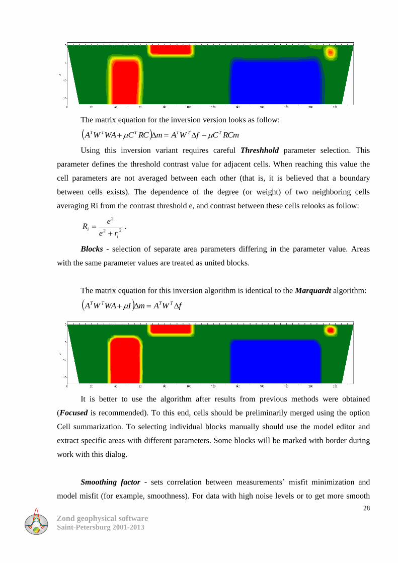
The matrix equation for the inversion version looks as follow:
RCmCfWAmRCCWAWA TTTTTT
Using this inversion variant requires careful Threshhold parameter selection. This
parameter defines the threshold contrast value for adjacent cells. When reaching this value the
cell parameters are not averaged between each other (that is, it is believed that a boundary
between cells exists). The dependence of the degree (or weight) of two neighboring cells
averaging Ri from the contrast threshold e, and contrast between these cells relooks as follow:
22
2
i
ire
eR
.
Blocks - selection of separate area parameters differing in the parameter value. Areas
with the same parameter values are treated as united blocks.
The matrix equation for this inversion algorithm is identical to the Marquardt algorithm:
fWAmIWAWA TTTT
It is better to use the algorithm after results from previous methods were obtained
(Focused is recommended). To this end, cells should be preliminarily merged using the option
Cell summarization. To selecting individual blocks manually should use the model editor and
extract specific areas with different parameters. Some blocks will be marked with border during
work with this dialog.
Smoothing factor - sets correlation between measurements’ misfit minimization and
model misfit (for example, smoothness). For data with high noise levels or to get more smooth
Zond geophysical software Saint-Petersburg 2001-2013
29
and stable distribution of parameters, relatively large values of smoothing parameter (0.5 – 2)
should be selected; for high quality data values : 0.005 - 0.01 can be used. As a rule, large values
of data misfit are obtained for large values of smoothing parameter. It is used in inversion
algorithms Occam and Focused.
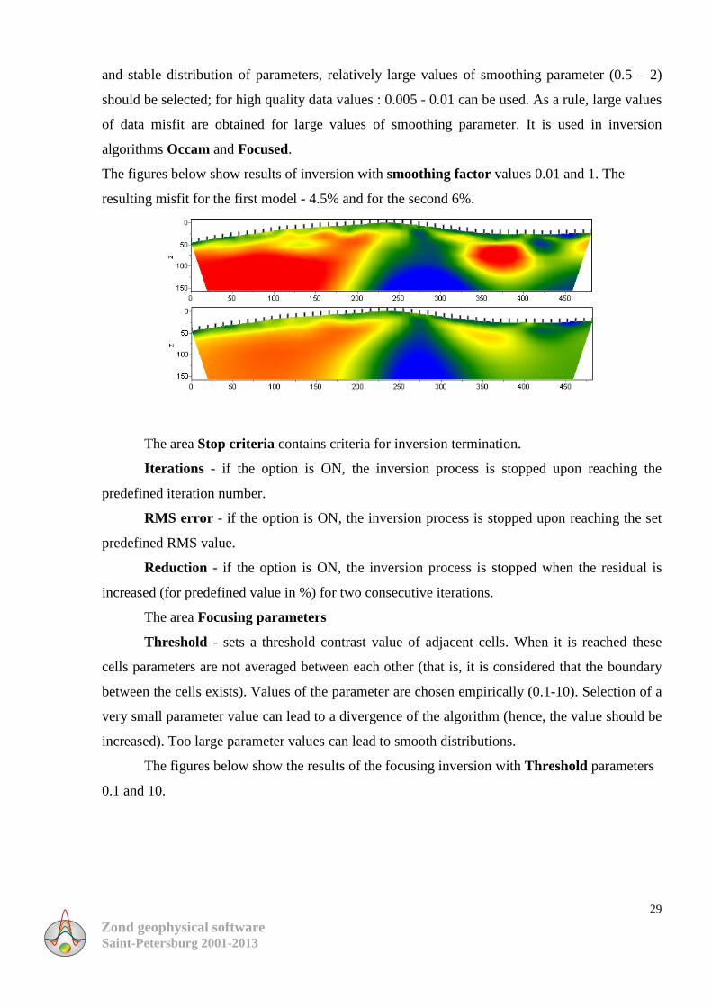
The figures below show results of inversion with smoothing factor values 0.01 and 1. The
resulting misfit for the first model - 4.5% and for the second 6%.
The area Stop criteria contains criteria for inversion termination.
Iterations - if the option is ON, the inversion process is stopped upon reaching the
predefined iteration number.
RMS error - if the option is ON, the inversion process is stopped upon reaching the set
predefined RMS value.
Reduction - if the option is ON, the inversion process is stopped when the residual is
increased (for predefined value in %) for two consecutive iterations.
The area Focusing parameters
Threshold - sets a threshold contrast value of adjacent cells. When it is reached these
cells parameters are not averaged between each other (that is, it is considered that the boundary
between the cells exists). Values of the parameter are chosen empirically (0.1-10). Selection of a
very small parameter value can lead to a divergence of the algorithm (hence, the value should be
increased). Too large parameter values can lead to smooth distributions.
The figures below show the results of the focusing inversion with Threshold parameters
0.1 and 10.
Zond geophysical software Saint-Petersburg 2001-2013
30
The figures below show the results of the focusing inversion with Threshold parameters
0.1 and 10.
Robust weighting scheme - this option should be switched ON if data contains some
spikes related to the systematic measurement errors. If amount of invalid data is comparable with
amount of valid measurements, the algorithm may not produce feasible results.
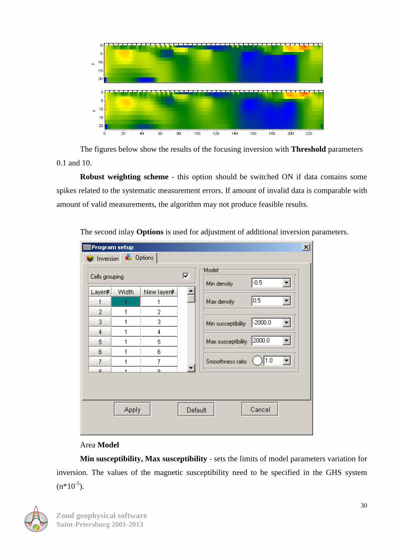
The second inlay Options is used for adjustment of additional inversion parameters.
Area Model
Min susceptibility, Max susceptibility - sets the limits of model parameters variation for
inversion. The values of the magnetic susceptibility need to be specified in the GHS system
(n*10-5
).
Zond geophysical software Saint-Petersburg 2001-2013
31
Min density, Max density - sets the limits of variation of the model parameters for
inversion. Density values need to be specified in g / cm3.
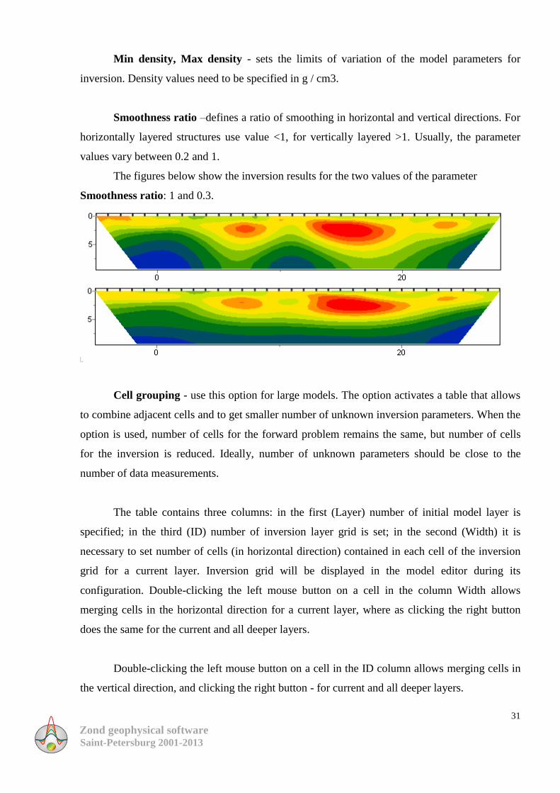
Smoothness ratio –defines a ratio of smoothing in horizontal and vertical directions. For
horizontally layered structures use value <1, for vertically layered >1. Usually, the parameter
values vary between 0.2 and 1.
The figures below show the inversion results for the two values of the parameter
Smoothness ratio: 1 and 0.3.
Cell grouping - use this option for large models. The option activates a table that allows
to combine adjacent cells and to get smaller number of unknown inversion parameters. When the
option is used, number of cells for the forward problem remains the same, but number of cells
for the inversion is reduced. Ideally, number of unknown parameters should be close to the
number of data measurements.
The table contains three columns: in the first (Layer) number of initial model layer is
specified; in the third (ID) number of inversion layer grid is set; in the second (Width) it is
necessary to set number of cells (in horizontal direction) contained in each cell of the inversion
grid for a current layer. Inversion grid will be displayed in the model editor during its
configuration. Double-clicking the left mouse button on a cell in the column Width allows
merging cells in the horizontal direction for a current layer, where as clicking the right button
does the same for the current and all deeper layers.
Double-clicking the left mouse button on a cell in the ID column allows merging cells in
the vertical direction, and clicking the right button - for current and all deeper layers.
Zond geophysical software Saint-Petersburg 2001-2013
32
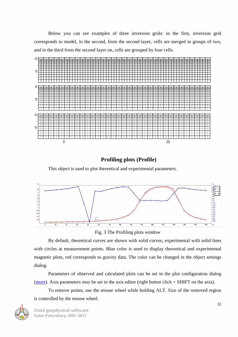
Below you can see examples of three inversion grids: in the first, inversion grid
corresponds to model, in the second, from the second layer, cells are merged in groups of two,
and in the third from the second layer on, cells are grouped by four cells.
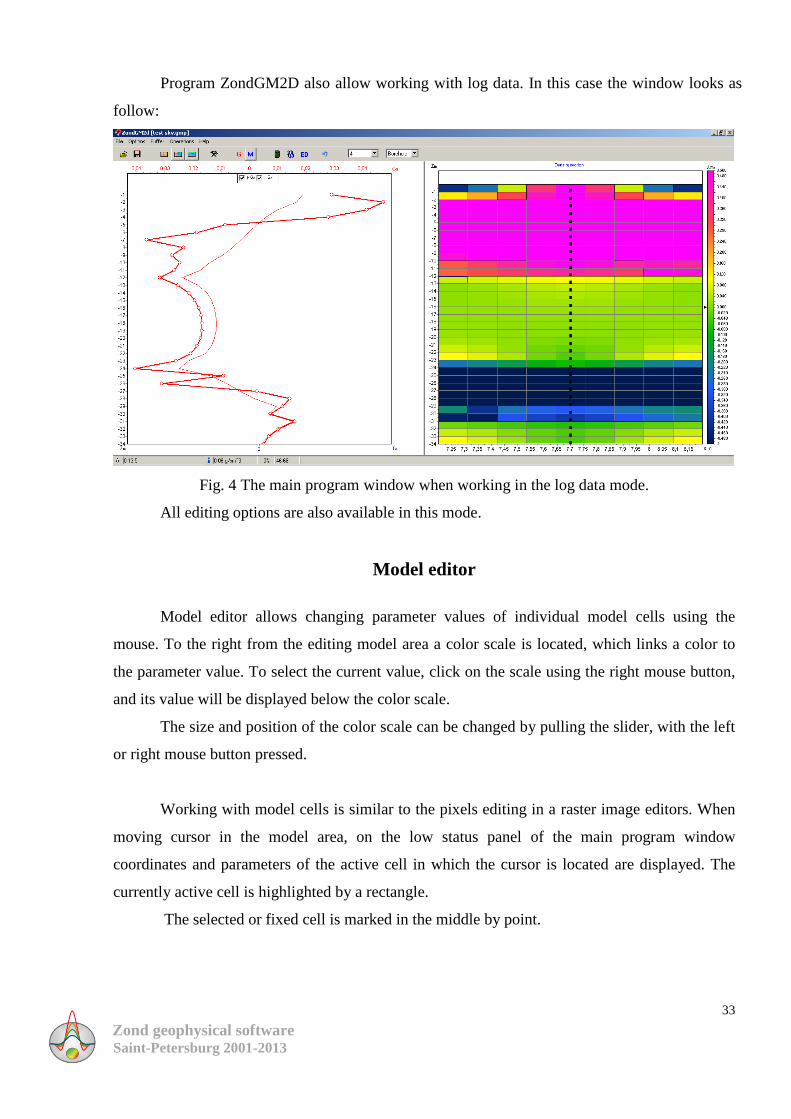
Profiling plots (Profile)
This object is used to plot theoretical and experimental parameters.
Fig. 3 The Profiling plots window
By default, theoretical curves are shown with solid curves, experimental with solid lines
with circles at measurement points. Blue color is used to display theoretical and experimental
magnetic plots, red corresponds to gravity data. The color can be changed in the object settings
dialog.
Parameters of observed and calculated plots can be set in the plot configuration dialog
(more). Axis parameters may be set in the axis editor (right button click + SHIFT on the axis).
To remove points, use the mouse wheel while holding ALT. Size of the removed region
is controlled by the mouse wheel.
Zond geophysical software Saint-Petersburg 2001-2013
33
Program ZondGM2D also allow working with log data. In this case the window looks as
follow:
Fig. 4 The main program window when working in the log data mode.
All editing options are also available in this mode.
Model editor
Model editor allows changing parameter values of individual model cells using the
mouse. To the right from the editing model area a color scale is located, which links a color to
the parameter value. To select the current value, click on the scale using the right mouse button,
and its value will be displayed below the color scale.
The size and position of the color scale can be changed by pulling the slider, with the left
or right mouse button pressed.
Working with model cells is similar to the pixels editing in a raster image editors. When
moving cursor in the model area, on the low status panel of the main program window
coordinates and parameters of the active cell in which the cursor is located are displayed. The
currently active cell is highlighted by a rectangle.
The selected or fixed cell is marked in the middle by point.
Zond geophysical software Saint-Petersburg 2001-2013
34
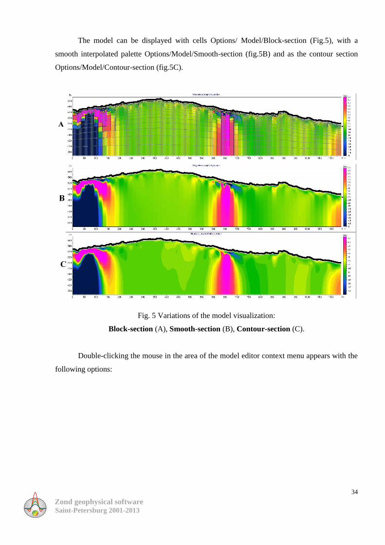
The model can be displayed with cells Options/ Model/Block-section (Fig.5), with a
smooth interpolated palette Options/Model/Smooth-section (fig.5B) and as the contour section
Options/Model/Contour-section (fig.5C).
Fig. 5 Variations of the model visualization:
Block-section (A), Smooth-section (B), Contour-section (C).
Double-clicking the mouse in the area of the model editor context menu appears with the
following options:

Zond geophysical software Saint-Petersburg 2001-2013
35
The top area Display model mesh Indicates whether to display model mesh.
Display objects
border
Indicates whether to display objects
border.
Display color bar Indicates whether to display color bar
Setup Show dialog of model parameters setup
(more).
Zoom&Scroll Switch on zoom and scroll mode.
Print preview Print the model.
Color bar Setup Show dialog of color bar setup.
Set minimum Set the minimum value of color bar.
Set maximum Set the maximum value of color bar.
Set incremental factor Set minimum and maximum values of the
color bar relative to background medium
value.
Automatic Determine the minimum and maximum
values of the color bar automatically.
Log scale Set logarithmic scale for the color bar.
Set cursor value Setthe current parameter value.
Colors as histogram Display color bar as histogram.
Vertical axis Set maximum Set depth value of the bottom layer.
Redivide Assign the same layer thicknesses for all
model layers (in current scale).
Thick mesh Remove every second node of the vertical
grid.
Thin mesh Add intermediate nodes in the vertical
grid.
Horizontal axis Redivide Set the same width for cells located
between the unique positions of
measurement points.
Thick mesh Remove every second node of the
Zond geophysical software Saint-Petersburg 2001-2013
36
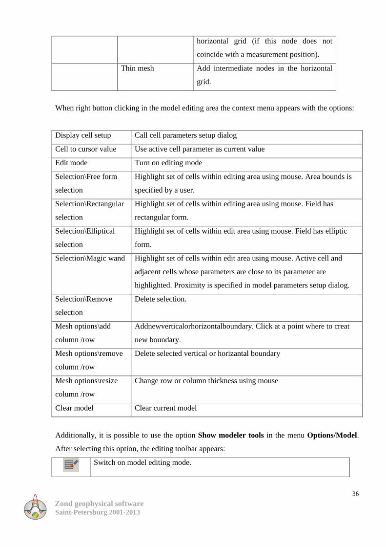
When right button clicking in the model editing area the context menu appears with the options:
Display cell setup Call cell parameters setup dialog
Cell to cursor value Use active cell parameter as current value
Edit mode Turn on editing mode
Selection\Free form
selection
Highlight set of cells within editing area using mouse. Area bounds is
specified by a user.
Selection\Rectangular
selection
Highlight set of cells within editing area using mouse. Field has
rectangular form.
Selection\Elliptical
selection
Highlight set of cells within edit area using mouse. Field has elliptic
form.
Selection\Magic wand Highlight set of cells within edit area using mouse. Active cell and
adjacent cells whose parameters are close to its parameter are
highlighted. Proximity is specified in model parameters setup dialog.
Selection\Remove
selection
Delete selection.
Mesh options\add
column /row
Addnewverticalorhorizontalboundary. Click at a point where to creat
new boundary.
Mesh options\remove
column /row
Delete selected vertical or horizantal boundary
Mesh options\resize
column /row
Change row or column thickness using mouse
Clear model Clear current model
Additionally, it is possible to use the option Show modeler tools in the menu Options/Model.
After selecting this option, the editing toolbar appears:
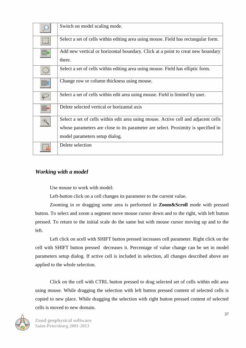
Switch on model editing mode.
horizontal grid (if this node does not
coincide with a measurement position).
Thin mesh Add intermediate nodes in the horizontal
grid.
Zond geophysical software Saint-Petersburg 2001-2013
37
Switch on model scaling mode.
Select a set of cells within editing area using mouse. Field has rectangular form.
Add new vertical or horizontal boundary. Click at a point to creat new boundary
there.
Select a set of cells within editing area using mouse. Field has elliptic form.
Change row or column thickness using mouse.
Select a set of cells within edit area using mouse. Field is limited by user.
Delete selected vertical or horizantal axis
Select a set of cells within edit area using mouse. Active cell and adjacent cells
whose parameters are close to its parameter are select. Proximity is specified in
model parameters setup dialog.
Delete selection
Working with a model
Use mouse to work with model:
Left-button click on a cell changes its parameter to the current value.
Zooming in or dragging some area is performed in Zoom&Scroll mode with pressed
button. To select and zoom a segment move mouse cursor down and to the right, with left button
pressed. To return to the initial scale do the same but with mouse cursor moving up and to the
left.
Left click on acell with SHIFT button pressed increases cell parameter. Right click on the
cell with SHIFT button pressed decreases it. Percentage of value change can be set in model
parameters setup dialog. If active cell is included in selection, all changes described above are
applied to the whole selection.
Click on the cell with CTRL button pressed to drag selected set of cells within edit area
using mouse. While dragging the selection with left button pressed content of selected cells is
copied to new place. While dragging the selection with right button pressed content of selected
cells is moved to new domain.

Zond geophysical software Saint-Petersburg 2001-2013
38
Dialog of model settings
Called by right-clicking in area of model in the drop-down menu option Setup.
Options tab
The area Box margins (pixels)
Left margin - sets an indent (in pixels) for figure from the left window margin.
Right margin - sets an indent (in pixels) for figure from the right window margin.
Top margin - sets an indent (in pixels) for figure from the top window margin.
Bottom margin - sets an indent (in pixels) for figure from the bottom window margin.
Object difference - sets the maximum value of ratio parameters of adjacent cells, above which a
border between them is drawn.
Selection admissibility - sets an acceptable level of parameter differences between adjacent
cells, with which cells are a single object and they are being selected together (in the selection
mode Magic Wand).
Parameter alteration - determines value of augment to parameters of the selected cells (in
percentage terms relative to value of the parameter) when working in mode Edit with the bottom
Shift pressed.
Font button calls font settings dialog.
Colors tab

Zond geophysical software Saint-Petersburg 2001-2013
39
Area Color bar
Palette button calls fill settings dialog (more)
Area Others
Body border - allows specifying color of border between adjacent cells, if a difference degree
between them is greater than the set value in option Parameter alteration.
Grid - sets grid color.
Selection – sets label color of the selected cell.
Fixed - sets label color of the fixed cell.
Cell parameters setup dialog
Called by right-clicking mouse in cell area, the drop-down menu option Display cell Setup.
This dialog serves for selecting cell parameters or highlights it.
Value – sets cell parameter value.
Fixed – fixes or frees cell parameter.
Min value, Max value– sets cell parameter size of changing.
Apply to selected – uses current settings for all selected cells if this function is ON.
Zond geophysical software Saint-Petersburg 2001-2013
40
Selection of medium model in inversion (modes of regular cells grid, polygonal
and randomly layered medium)
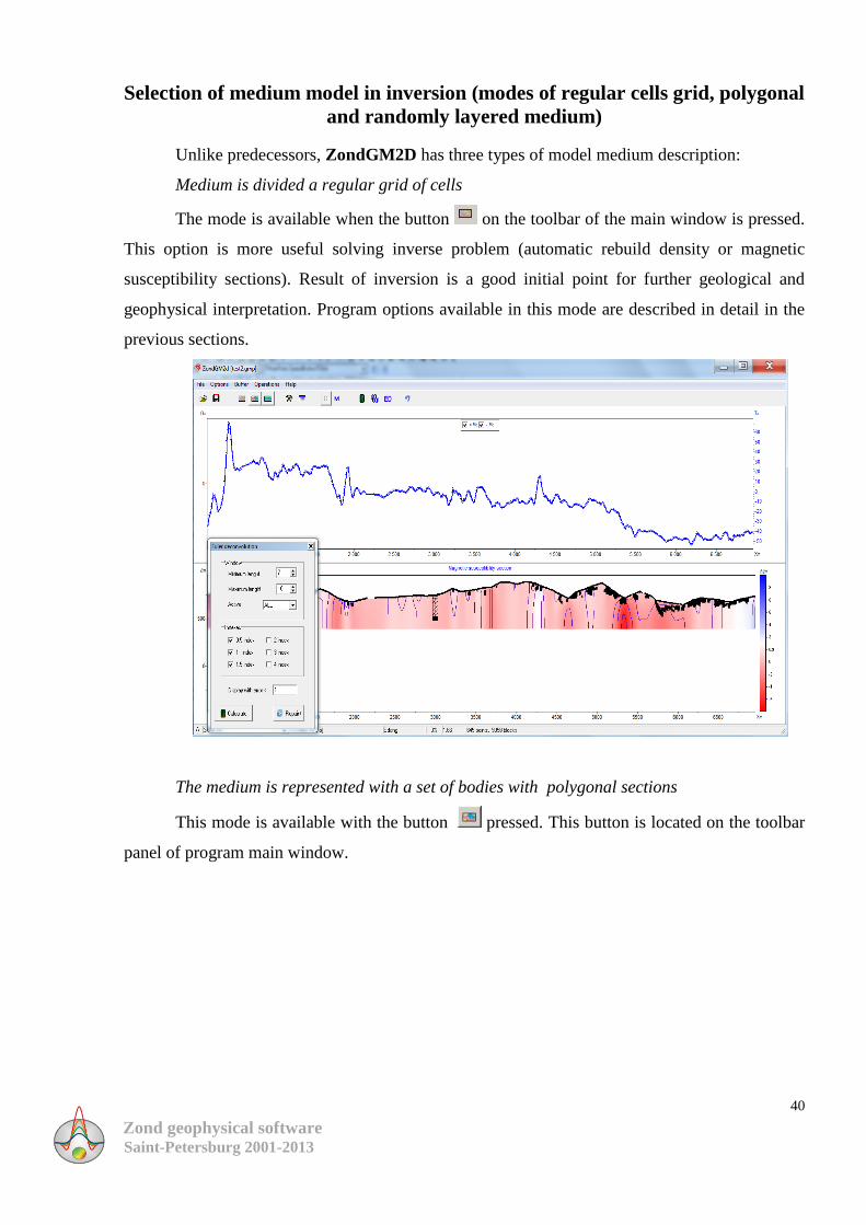
Unlike predecessors, ZondGM2D has three types of model medium description:
Medium is divided a regular grid of cells
The mode is available when the button on the toolbar of the main window is pressed.
This option is more useful solving inverse problem (automatic rebuild density or magnetic
susceptibility sections). Result of inversion is a good initial point for further geological and
geophysical interpretation. Program options available in this mode are described in detail in the
previous sections.
The medium is represented with a set of bodies with polygonal sections
This mode is available with the button pressed. This button is located on the toolbar
panel of program main window.

Zond geophysical software Saint-Petersburg 2001-2013
41
Polygonal approach of petrophysical medium description aids more structural approach
to the data interpretation. Using this approach two-dimensional section of every body
representing a section, is described as a closed polygon. Model construction is done by building
a set of polygons with arbitrary geometry, with specified magnetic and density parameters. It is
the most convenient option for the final stage of interpretation. ZondGM2D has a large set of
tools to quickly create models of any complexity. Details about the set of tools are given in the
part Modeling.
Solution of the inverse problem for polygonal model variant means an automatic
correction of polygon node positions and its petrophysical parameters. When clicking on
inversion bottom pop-up menu appears and it contains following options:
Par inversion - parameters identification (magnetic susceptibility and density) of
polygons without changing the polygon nodes position
Z nodes inversion –fittingvertical position of polygon nodes
X nodes inversion – fitting horizontal position of polygon nodes
ZX nodes inversion –fitting polygons geometry
PZX inversion - fitting parameters and geometry of polygons
For this model type joint gravity and magnetic data fitting is available.
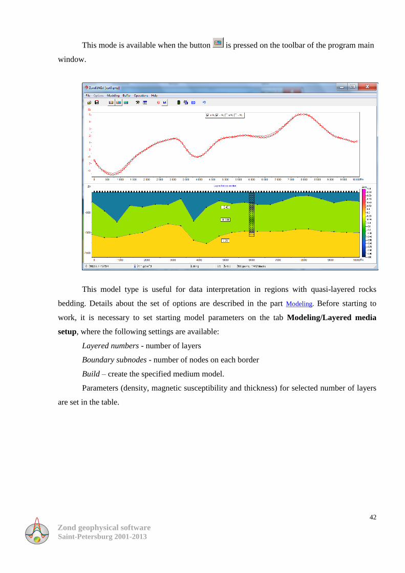
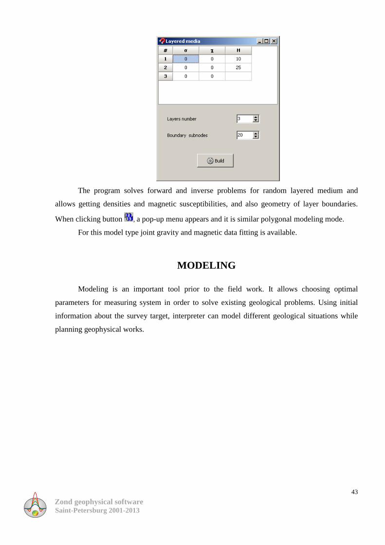
Arbitrary layered medium
Zond geophysical software Saint-Petersburg 2001-2013
42
This mode is available when the button is pressed on the toolbar of the program main
window.
This model type is useful for data interpretation in regions with quasi-layered rocks
bedding. Details about the set of options are described in the part Modeling. Before starting to
work, it is necessary to set starting model parameters on the tab Modeling/Layered media
setup, where the following settings are available:
Layered numbers - number of layers
Boundary subnodes - number of nodes on each border
Build – create the specified medium model.
Parameters (density, magnetic susceptibility and thickness) for selected number of layers
are set in the table.
Zond geophysical software Saint-Petersburg 2001-2013
43
The program solves forward and inverse problems for random layered medium and
allows getting densities and magnetic susceptibilities, and also geometry of layer boundaries.
When clicking button , a pop-up menu appears and it is similar polygonal modeling mode.
For this model type joint gravity and magnetic data fitting is available.
MODELING
Modeling is an important tool prior to the field work. It allows choosing optimal
parameters for measuring system in order to solve existing geological problems. Using initial
information about the survey target, interpreter can model different geological situations while
planning geophysical works.
Zond geophysical software Saint-Petersburg 2001-2013
44
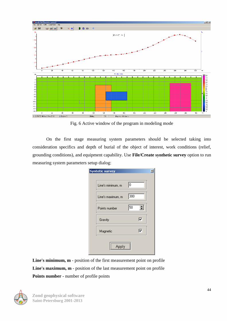
Fig. 6 Active window of the program in modeling mode
On the first stage measuring system parameters should be selected taking into
consideration specifics and depth of burial of the object of interest, work conditions (relief,
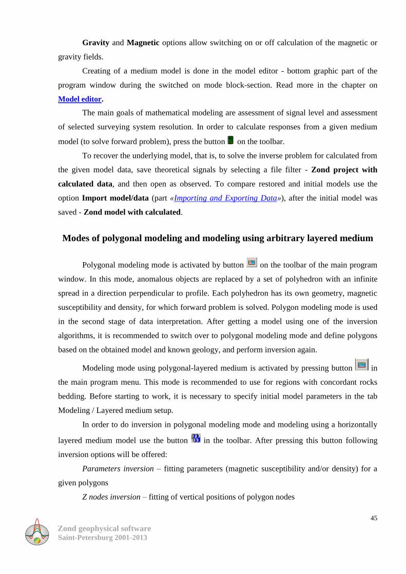
grounding conditions), and equipment capability. Use File/Create synthetic survey option to run
measuring system parameters setup dialog:
Line's minimum, m - position of the first measurement point on profile
Line's maximum, m - position of the last measurement point on profile
Points number - number of profile points
Zond geophysical software Saint-Petersburg 2001-2013
45
Gravity and Magnetic options allow switching on or off calculation of the magnetic or
gravity fields.
Creating of a medium model is done in the model editor - bottom graphic part of the
program window during the switched on mode block-section. Read more in the chapter on
Model editor.
The main goals of mathematical modeling are assessment of signal level and assessment
of selected surveying system resolution. In order to calculate responses from a given medium
model (to solve forward problem), press the button on the toolbar.
To recover the underlying model, that is, to solve the inverse problem for calculated from
the given model data, save theoretical signals by selecting a file filter - Zond project with
calculated data, and then open as observed. To compare restored and initial models use the
option Import model/data (part «Importing and Exporting Data»), after the initial model was
saved - Zond model with calculated.
Modes of polygonal modeling and modeling using arbitrary layered medium
Polygonal modeling mode is activated by button on the toolbar of the main program
window. In this mode, anomalous objects are replaced by a set of polyhedron with an infinite
spread in a direction perpendicular to profile. Each polyhedron has its own geometry, magnetic
susceptibility and density, for which forward problem is solved. Polygon modeling mode is used
in the second stage of data interpretation. After getting a model using one of the inversion
algorithms, it is recommended to switch over to polygonal modeling mode and define polygons
based on the obtained model and known geology, and perform inversion again.
Modeling mode using polygonal-layered medium is activated by pressing button in
the main program menu. This mode is recommended to use for regions with concordant rocks
bedding. Before starting to work, it is necessary to specify initial model parameters in the tab
Modeling / Layered medium setup.
In order to do inversion in polygonal modeling mode and modeling using a horizontally
layered medium model use the button in the toolbar. After pressing this button following
inversion options will be offered:
Parameters inversion – fitting parameters (magnetic susceptibility and/or density) for a
given polygons
Z nodes inversion – fitting of vertical positions of polygon nodes
Zond geophysical software Saint-Petersburg 2001-2013
46
X nodes inversion – fitting of horizontal positions of polygon nodes
ZX nodes inversion – fitting positions of nodes of specified polygons
PZX inversion – fitting parameters (magnetic susceptibility and/or density) and node
positions of specified polygons.
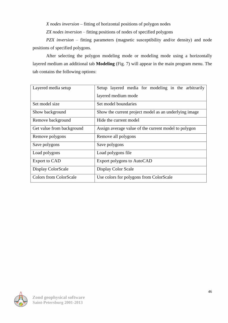
After selecting the polygon modeling mode or modeling mode using a horizontally
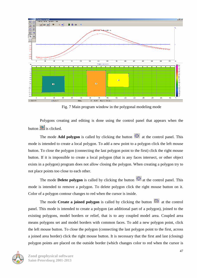
layered medium an additional tab Modeling (Fig. 7) will appear in the main program menu. The
tab contains the following options:
Layered media setup Setup layered media for modeling in the arbitrarily
layered medium mode
Set model size Set model boundaries
Show background Show the current project model as an underlying image
Remove background Hide the current model
Get value from background Assign average value of the current model to polygon
Remove polygons Remove all polygons
Save polygons Save polygons
Load polygons Load polygons file
Export to CAD Export polygons to AutoCAD
Display ColorScale Display Color Scale
Colors from ColorScale Use colors for polygons from ColorScale
Zond geophysical software Saint-Petersburg 2001-2013
47
Fig. 7 Main program window in the polygonal modeling mode
Polygons creating and editing is done using the control panel that appears when the
button is clicked.
The mode Add polygon is called by clicking the button at the control panel. This
mode is intended to create a local polygon. To add a new point to a polygon click the left mouse
button. To close the polygon (connecting the last polygon point to the first) click the right mouse
button. If it is impossible to create a local polygon (that is any faces intersect, or other object
exists in a polygon) program does not allow closing the polygon. When creating a polygon try to
not place points too close to each other.
The mode Delete polygon is called by clicking the button at the control panel. This
mode is intended to remove a polygon. To delete polygon click the right mouse button on it.
Color of a polygon contour changes to red when the cursor is inside.
The mode Create a joined polygon is called by clicking the button at the control
panel. This mode is intended to create a polygon (an additional part of a polygon), joined to the
existing polygons, model borders or relief, that is to any coupled model area. Coupled area
means polygons set and model borders with common faces. To add a new polygon point, click
the left mouse button. To close the polygon (connecting the last polygon point to the first, across
a joined area border) click the right mouse button. It is necessary that the first and last (closing)
polygon points are placed on the outside border (which changes color to red when the cursor is
Zond geophysical software Saint-Petersburg 2001-2013
48
approaching) of a coupled area. If it is impossible to create a local polygon (that is any faces
intersect, or other object exists in a polygon) program does not allow user to close the polygon
and remove all created points. Note that polygons joined to the left, right and bottom edges of the
model have infinite strike in those directions (that is they extend beyond the model).
The mode Disconnect polygon is called by clicking the button at the control panel.
This mode is intended to disconnect a polygon from a set of adjoint polygons or model edges.
Polygon disconnected from the model edges loses its infinite strike (it will be limited by the
model). To disconnect a polygon click the right mouse button on it. Color of the polygon contour
changes to red when the cursor is inside. Further, using the button Move polygon, it is possible
to move disconnected polygon part from the main polygon.
The mode Split polygon is used to create two parts inside a polygon. It is called by
clicking the button on the control panel. The mode is intended to split the polygon into two
new connected polygons. The interface is defined by two points at borders or nodes of the
polygon, which is split. To select the first border point click the left mouse button. To select the
second point and to split polygon click the right mouse button. If the operation is impossible
(that is any faces intersect, or border is outside the polygon) program does not allow user to split
the polygon and remove the created border. Color of the borders and points of a polygon changes
to red when the cursor is approaching.
The mode Move polygon is called by clicking the button on the control panel. This
mode is intended to move unconnected polygon points. If a polygon has no common,
unconnected with other polygons or model borders points, then it is moved completely. To select
a polygon being moved click the left mouse button; after that an unconnected polygon part is
moved with the cursor. To fix new position of the polygon click the right mouse button. If the
operation is impossible (that is any borders intersect, or a polygon exists in other polygon)
program does not allow user to move the polygon and return it to the original position. Color of
the polygon contour changes to red when the cursor is inside.
The mode Move connected polygons is called by clicking the button on the control
panel. This mode is intended to move a polygon and all connected with it. To select a polygon
being moved, click the left mouse button; after that the connected area moves with the cursor. To
fix new position of polygons click the right mouse button. If the operation is impossible (that is
any borders intersect, or a polygon exists in other polygon) program does not allow user to move
Zond geophysical software Saint-Petersburg 2001-2013
49
the polygons and return them to original positions. Color of the polygon contour changes to red
when the cursor is inside.
The mode Add point is called by clicking the button on the control panel. This mode is
intended to add a new point on a border of an existing polygon. To add a polygon point, click the
right mouse button on its border. Color of the polygon borders change to red when the cursor is
approaching.
The mode Remove point is called by clicking the button on the control panel. This
mode is intended to remove new point of existing polygon. To remove a polygon point, click the
right mouse button on it. The operation is impossible in the next cases: borders intersect, a
polygon is in other one or number of polygon points is less than three. Color of polygon points
changes to red when the cursor is approaching.
The mode Merge points is called by clicking the button on the control panel. This
mode is intended to merge two points into one by joining points to the border of another
polygon, or to the model edges. Selection of the first merging point.
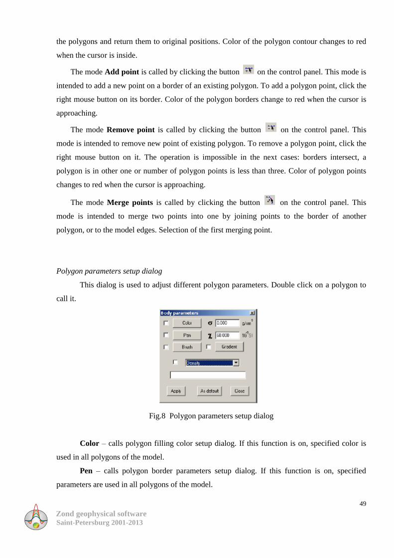
Polygon parameters setup dialog
This dialog is used to adjust different polygon parameters. Double click on a polygon to
call it.
Fig.8 Polygon parameters setup dialog
Color – calls polygon filling color setup dialog. If this function is on, specified color is
used in all polygons of the model.
Pen – calls polygon border parameters setup dialog. If this function is on, specified
parameters are used in all polygons of the model.
Zond geophysical software Saint-Petersburg 2001-2013
50
Brush – calls polygon filling setup dialog. If this function is on, specified parameters are
used in all polygons of the model.
Gradient – calls polygon gradient filling setup dialog. If this function is on, specified
parameters are used in all polygons of the model.
– sets polygon density value.
– sets polygon magnetic susceptibility value.
The following option specifies type of label displayed on a polygon. If this function is on,
specified type is used in all polygons of the model.
Value None – there is no label on a polygon.
Value Density – polygon density value is displayed on a polygon.
Value Susceptibility – polygon magnetic susceptibility value is displayed on polygon.
Value Density & Susceptibility – polygon density and magnetic susceptibility values are
displayed on a polygon.
Value User text – value of the following field is displayed on polygon. The following option
specifies type of label displayed on a polygon. If this function is on, specified type is used in all
polygons of the model.
ADVANCED PROGRAM OPTIONS
Euler deconvolution
In addition to inversion, Euler deconvolution is available in ZondGM2D. The option
allows getting distribution of magnetic and gravity sources (special points). This option is
activated by clicking a button on the toolbar of the main program window, then the
following dialog box appears:
Zond geophysical software Saint-Petersburg 2001-2013
51
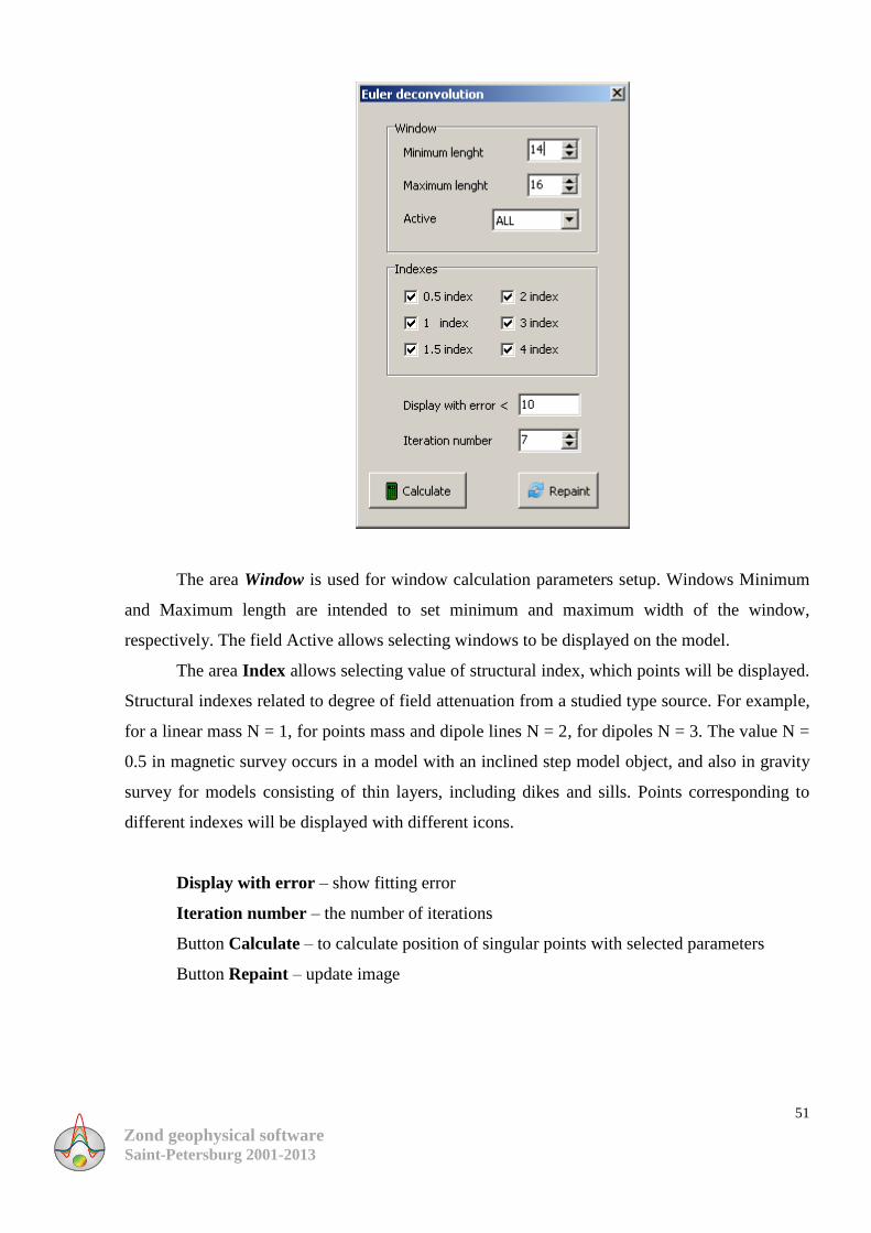
The area Window is used for window calculation parameters setup. Windows Minimum
and Maximum length are intended to set minimum and maximum width of the window,
respectively. The field Active allows selecting windows to be displayed on the model.
The area Index allows selecting value of structural index, which points will be displayed.
Structural indexes related to degree of field attenuation from a studied type source. For example,
for a linear mass N = 1, for points mass and dipole lines N = 2, for dipoles N = 3. The value N =
0.5 in magnetic survey occurs in a model with an inclined step model object, and also in gravity
survey for models consisting of thin layers, including dikes and sills. Points corresponding to
different indexes will be displayed with different icons.
Display with error – show fitting error
Iteration number – the number of iterations
Button Calculate – to calculate position of singular points with selected parameters
Button Repaint – update image
Zond geophysical software Saint-Petersburg 2001-2013
52
Downward continuation
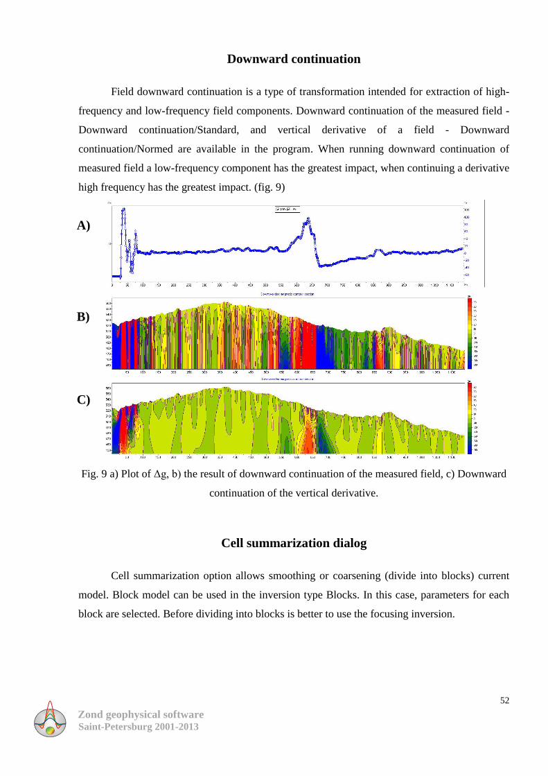
Field downward continuation is a type of transformation intended for extraction of high-
frequency and low-frequency field components. Downward continuation of the measured field -
Downward continuation/Standard, and vertical derivative of a field - Downward
continuation/Normed are available in the program. When running downward continuation of
measured field a low-frequency component has the greatest impact, when continuing a derivative
high frequency has the greatest impact. (fig. 9)
Fig. 9 a) Plot of Δg, b) the result of downward continuation of the measured field, c) Downward
continuation of the vertical derivative.
Cell summarization dialog
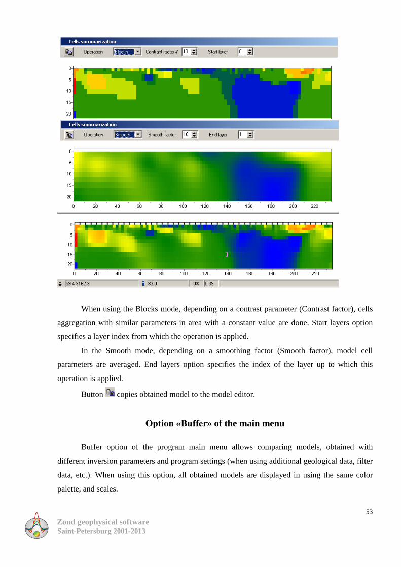
Cell summarization option allows smoothing or coarsening (divide into blocks) current
model. Block model can be used in the inversion type Blocks. In this case, parameters for each
block are selected. Before dividing into blocks is better to use the focusing inversion.
A)
B)
C)
Zond geophysical software Saint-Petersburg 2001-2013
53
When using the Blocks mode, depending on a contrast parameter (Contrast factor), cells
aggregation with similar parameters in area with a constant value are done. Start layers option
specifies a layer index from which the operation is applied.
In the Smooth mode, depending on a smoothing factor (Smooth factor), model cell
parameters are averaged. End layers option specifies the index of the layer up to which this
operation is applied.
Button copies obtained model to the model editor.
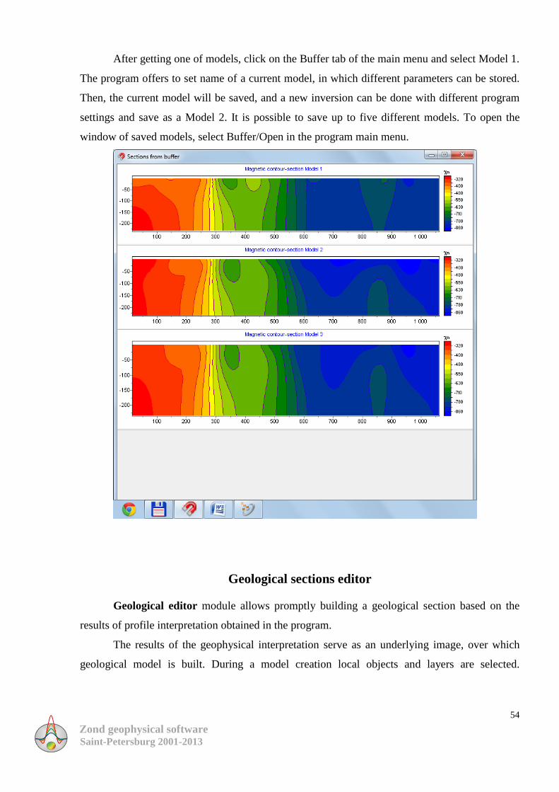
Option «Buffer» of the main menu
Buffer option of the program main menu allows comparing models, obtained with
different inversion parameters and program settings (when using additional geological data, filter
data, etc.). When using this option, all obtained models are displayed in using the same color
palette, and scales.
Zond geophysical software Saint-Petersburg 2001-2013
54
After getting one of models, click on the Buffer tab of the main menu and select Model 1.
The program offers to set name of a current model, in which different parameters can be stored.
Then, the current model will be saved, and a new inversion can be done with different program
settings and save as a Model 2. It is possible to save up to five different models. To open the
window of saved models, select Buffer/Open in the program main menu.
Geological sections editor
Geological editor module allows promptly building a geological section based on the
results of profile interpretation obtained in the program.
The results of the geophysical interpretation serve as an underlying image, over which
geological model is built. During a model creation local objects and layers are selected.
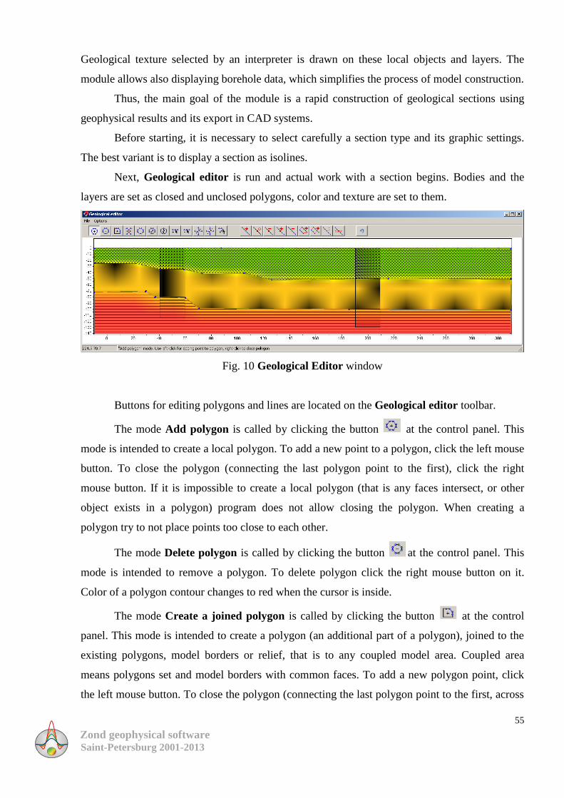
Zond geophysical software Saint-Petersburg 2001-2013
55
Geological texture selected by an interpreter is drawn on these local objects and layers. The
module allows also displaying borehole data, which simplifies the process of model construction.
Thus, the main goal of the module is a rapid construction of geological sections using
geophysical results and its export in CAD systems.
Before starting, it is necessary to select carefully a section type and its graphic settings.
The best variant is to display a section as isolines.
Next, Geological editor is run and actual work with a section begins. Bodies and the
layers are set as closed and unclosed polygons, color and texture are set to them.
Fig. 10 Geological Editor window
Buttons for editing polygons and lines are located on the Geological editor toolbar.
The mode Add polygon is called by clicking the button at the control panel. This
mode is intended to create a local polygon. To add a new point to a polygon, click the left mouse
button. To close the polygon (connecting the last polygon point to the first), click the right
mouse button. If it is impossible to create a local polygon (that is any faces intersect, or other
object exists in a polygon) program does not allow closing the polygon. When creating a
polygon try to not place points too close to each other.
The mode Delete polygon is called by clicking the button at the control panel. This
mode is intended to remove a polygon. To delete polygon click the right mouse button on it.
Color of a polygon contour changes to red when the cursor is inside.
The mode Create a joined polygon is called by clicking the button at the control
panel. This mode is intended to create a polygon (an additional part of a polygon), joined to the
existing polygons, model borders or relief, that is to any coupled model area. Coupled area
means polygons set and model borders with common faces. To add a new polygon point, click
the left mouse button. To close the polygon (connecting the last polygon point to the first, across
Zond geophysical software Saint-Petersburg 2001-2013
56
a joined area border), click the right mouse button. It is necessary that the first and last (closing)
polygon points are placed on the outside border (which changes color to red when the cursor is
approaching) of a coupled area. If it is impossible to create a local polygon (that is any faces
intersect, or other object exists in a polygon) program does not allow user to close the polygon
and remove all created points. Note that polygons joined to the left, right and bottom edges of the
model have infinite strike in those directions (that is they extend beyond the model).
The mode Disconnect polygon is called by clicking the button at the control panel.
This mode is intended to disconnect a polygon from a set of adjoint polygons or model edges.
Polygon disconnected from the model edges loses its infinite strike (it will be limited by the
model). To disconnect a polygon click the right mouse button on it. Color of the polygon contour
changes to red when the cursor is inside. Further, using the button Move polygon, it is possible
to move disconnected polygon part from the main polygon.
The mode Split polygon is intended to create two parts inside a polygon. It is called by
clicking the button on the control panel. The mode is intended to split the polygon into two
new connected polygons. The interface is defined by two points at borders or nodes of the
polygon, which is split. To select the first border point, click the left mouse button. To select the
second point and to split polygon, click the right mouse button. If the operation is impossible
(that is any faces intersect, or border is outside the polygon) program does not allow user to split
the polygon and remove the created border. Color of the borders and points of a polygon changes
to red when the cursor is approaching.
The mode Move polygon is called by clicking the button on the control panel. This
mode is intended to move unconnected polygon points. If a polygon has no common,
unconnected with other polygons or model borders points, then it is moved completely. To select
a polygon being moved, click the left mouse button; after that an unconnected polygon part is
moved with the cursor. To fix new position of the polygon click the right mouse button. If the
operation is impossible (that is any borders intersect, or a polygon exists in other polygon)
program does not allow user to move the polygon and return it to the original position. Color of
the polygon contour changes to red when the cursor is inside.
The mode Move connected polygons is called by clicking the button on the control
panel. This mode is intended to move a polygon and all connected with it. To select a polygon
being moved, click the left mouse button; after that the connected area moves with the cursor. To
fix new position of polygons click the right mouse button. If the operation is impossible (that is
Zond geophysical software Saint-Petersburg 2001-2013
57
any borders intersect, or a polygon exists in other polygon) program does not allow user to move
the polygons and return them to original positions. Color of the polygon contour changes to red
when the cursor is inside.
The mode Add point is called by clicking the button on the control panel. This
mode is intended to add a new point on a border of an existing polygon. To add a polygon point,
click the right mouse button on its border. Color of the polygon borders change to red when the
cursor is approaching.
The mode Remove point is called by clicking the button on the control panel. This
mode is intended to remove new point of existing polygon. To remove a polygon point, click the
right mouse button on it. The operation is impossible in the next cases: borders intersect, a
polygon is in other one or number of polygon points is less than three. Color of polygon points
changes to red when the cursor is approaching.
The mode Merge points is called by clicking the button on the control panel. This
mode is intended to merge two points into one by joining points to the border of another
polygon, or to the model edges. Selection of the first merging point
The mode Disconnect points is called by clicking the button on the control panel.
This mode is intended to disconnect previously merged points. To disconnect points of
connected polygon click the right mouse button on it. As a result of this operation, instead of one
connected point a set of disconnected points appears. Each point belongs to its own polygon.
Color of polygon points changes to red when the cursor is approaching.
The mode Move point is called by clicking the button on the control panel. This
mode is intended to move polygon point. To select moving point, click the left mouse button;
after that polygon point moves with the cursor. To fix position of the new point click the right
mouse button. If the operation is not possible (that is faces intersect) program does not allow you
to move a point and returns it to its original position. Points located on model boundaries are
moved only along appropriate edges. Color of polygon points changes to red when the cursor is
approaching.
Polygon parameters setup dialog
This dialog is used to adjust different polygon parameters. Double click on necessary
polygon to run it.
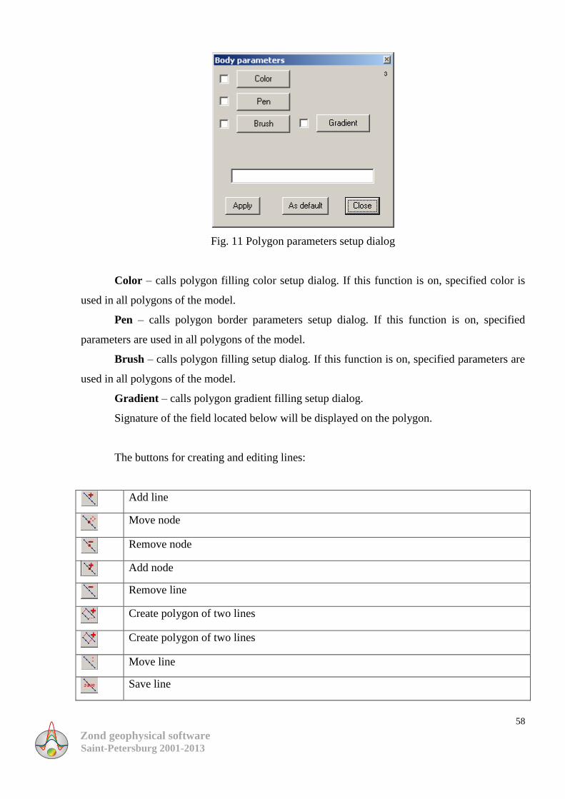
Zond geophysical software Saint-Petersburg 2001-2013
58
Fig. 11 Polygon parameters setup dialog
Color – calls polygon filling color setup dialog. If this function is on, specified color is
used in all polygons of the model.
Pen – calls polygon border parameters setup dialog. If this function is on, specified
parameters are used in all polygons of the model.
Brush – calls polygon filling setup dialog. If this function is on, specified parameters are
used in all polygons of the model.
Gradient – calls polygon gradient filling setup dialog.
Signature of the field located below will be displayed on the polygon.
The buttons for creating and editing lines:
Add line
Move node
Remove node
Add node
Remove line
Create polygon of two lines
Create polygon of two lines
Move line
Save line
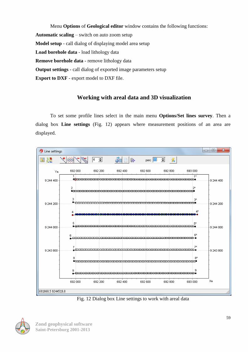
Zond geophysical software Saint-Petersburg 2001-2013
59
Menu Options of Geological editor window contains the following functions:
Automatic scaling – switch on auto zoom setup
Model setup - call dialog of displaying model area setup
Load borehole data - load lithology data
Remove borehole data - remove lithology data
Output settings - call dialog of exported image parameters setup
Export to DXF - export model to DXF file.
Working with areal data and 3D visualization
To set some profile lines select in the main menu Options/Set lines survey. Then a
dialog box Line settings (Fig. 12) appears where measurement positions of an area are
displayed.
Fig. 12 Dialog box Line settings to work with areal data
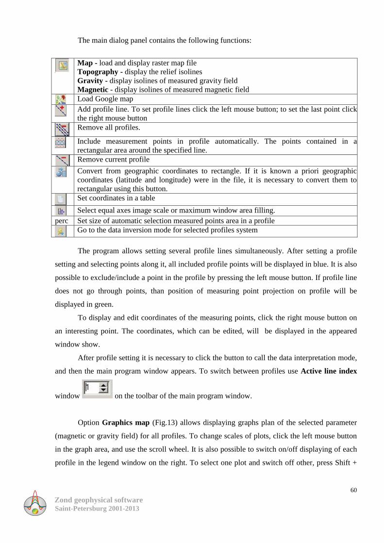
Zond geophysical software Saint-Petersburg 2001-2013
60
The main dialog panel contains the following functions:
Map - load and display raster map file
Topography - display the relief isolines
Gravity - display isolines of measured gravity field
Magnetic - display isolines of measured magnetic field
Load Google map
Add profile line. To set profile lines click the left mouse button; to set the last point click
the right mouse button
Remove all profiles.
Include measurement points in profile automatically. The points contained in a
rectangular area around the specified line.
Remove current profile
Convert from geographic coordinates to rectangle. If it is known a priori geographic
coordinates (latitude and longitude) were in the file, it is necessary to convert them to
rectangular using this button.
Set coordinates in a table
Select equal axes image scale or maximum window area filling.
perc Set size of automatic selection measured points area in a profile
Go to the data inversion mode for selected profiles system
The program allows setting several profile lines simultaneously. After setting a profile
setting and selecting points along it, all included profile points will be displayed in blue. It is also
possible to exclude/include a point in the profile by pressing the left mouse button. If profile line
does not go through points, than position of measuring point projection on profile will be
displayed in green.
To display and edit coordinates of the measuring points, click the right mouse button on
an interesting point. The coordinates, which can be edited, will be displayed in the appeared
window show.
After profile setting it is necessary to click the button to call the data interpretation mode,
and then the main program window appears. To switch between profiles use Active line index
window on the toolbar of the main program window.
Option Graphics map (Fig.13) allows displaying graphs plan of the selected parameter
(magnetic or gravity field) for all profiles. To change scales of plots, click the left mouse button
in the graph area, and use the scroll wheel. It is also possible to switch on/off displaying of each
profile in the legend window on the right. To select one plot and switch off other, press Shift +
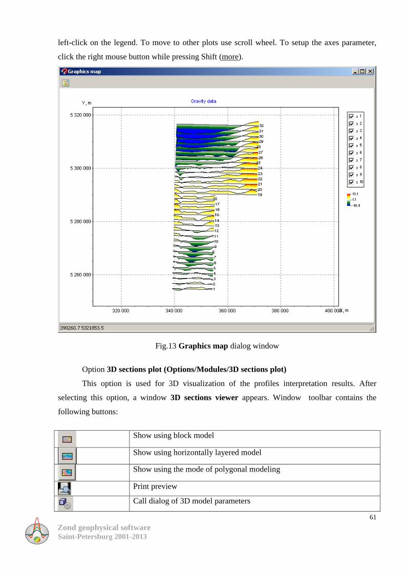
Zond geophysical software Saint-Petersburg 2001-2013
61
left-click on the legend. To move to other plots use scroll wheel. To setup the axes parameter,
click the right mouse button while pressing Shift (more).
Fig.13 Graphics map dialog window
Option 3D sections plot (Options/Modules/3D sections plot)
This option is used for 3D visualization of the profiles interpretation results. After
selecting this option, a window 3D sections viewer appears. Window toolbar contains the
following buttons:
Show using block model
Show using horizontally layered model
Show using the mode of polygonal modeling
Print preview
Call dialog of 3D model parameters
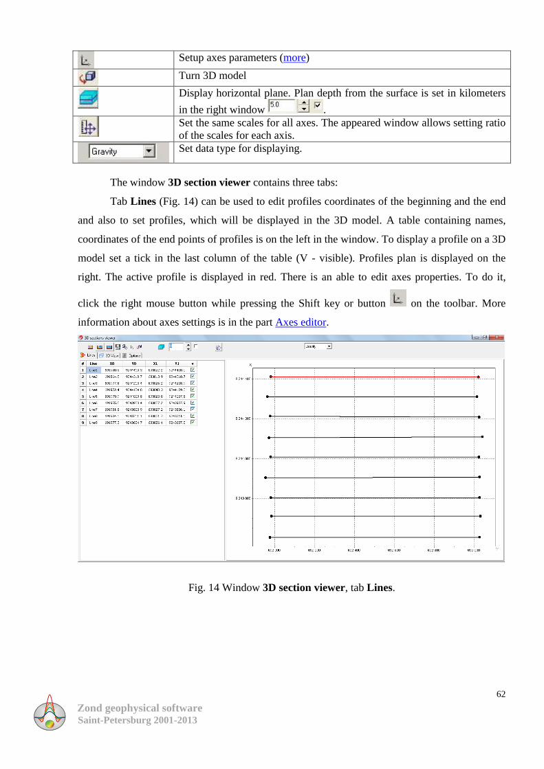
Zond geophysical software Saint-Petersburg 2001-2013
62
Setup axes parameters (more)
Turn 3D model
Display horizontal plane. Plan depth from the surface is set in kilometers
in the right window .
Set the same scales for all axes. The appeared window allows setting ratio
of the scales for each axis.
Set data type for displaying.
The window 3D section viewer contains three tabs:
Tab Lines (Fig. 14) can be used to edit profiles coordinates of the beginning and the end
and also to set profiles, which will be displayed in the 3D model. A table containing names,
coordinates of the end points of profiles is on the left in the window. To display a profile on a 3D
model set a tick in the last column of the table (V - visible). Profiles plan is displayed on the
right. The active profile is displayed in red. There is an able to edit axes properties. To do it,
click the right mouse button while pressing the Shift key or button on the toolbar. More
information about axes settings is in the part Axes editor.
Fig. 14 Window 3D section viewer, tab Lines.
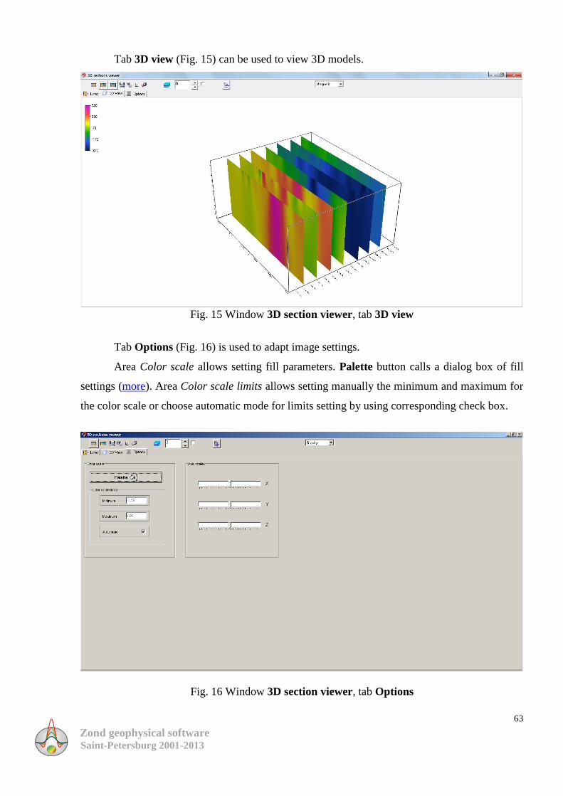
Zond geophysical software Saint-Petersburg 2001-2013
63
Tab 3D view (Fig. 15) can be used to view 3D models.
Fig. 15 Window 3D section viewer, tab 3D view
Tab Options (Fig. 16) is used to adapt image settings.
Area Color scale allows setting fill parameters. Palette button calls a dialog box of fill
settings (more). Area Color scale limits allows setting manually the minimum and maximum for
the color scale or choose automatic mode for limits setting by using corresponding check box.
Fig. 16 Window 3D section viewer, tab Options
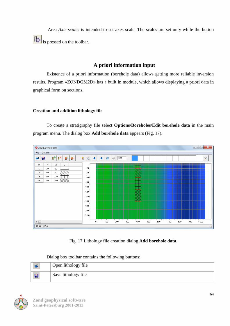
Zond geophysical software Saint-Petersburg 2001-2013
64
Area Axis scales is intended to set axes scale. The scales are set only while the button
is pressed on the toolbar.
A priori information input
Existence of a priori information (borehole data) allows getting more reliable inversion
results. Program «ZONDGM2D» has a built in module, which allows displaying a priori data in
graphical form on sections.
Creation and addition lithology file
To create a stratigraphy file select Options/Boreholes/Edit borehole data in the main
program menu. The dialog box Add borehole data appears (Fig. 17).
Fig. 17 Lithology file creation dialog Add borehole data.
Dialog box toolbar contains the following buttons:
Open lithology file
Save lithology file
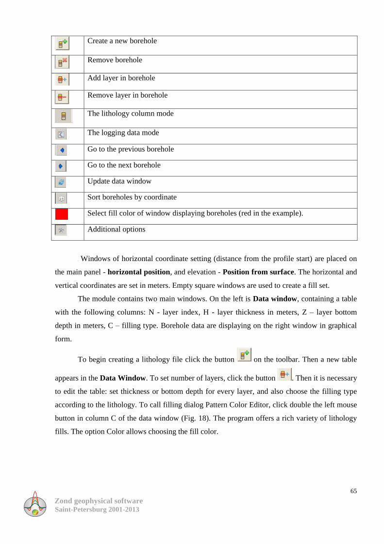
Zond geophysical software Saint-Petersburg 2001-2013
65
Create a new borehole
Remove borehole
Add layer in borehole
Remove layer in borehole
The lithology column mode
The logging data mode
Go to the previous borehole
Go to the next borehole
Update data window
Sort boreholes by coordinate
Select fill color of window displaying boreholes (red in the example).
Additional options
Windows of horizontal coordinate setting (distance from the profile start) are placed on
the main panel - horizontal position, and elevation - Position from surface. The horizontal and
vertical coordinates are set in meters. Empty square windows are used to create a fill set.
The module contains two main windows. On the left is Data window, containing a table
with the following columns: N - layer index, H - layer thickness in meters, Z – layer bottom
depth in meters, C – filling type. Borehole data are displaying on the right window in graphical
form.
To begin creating a lithology file click the button on the toolbar. Then a new table
appears in the Data Window. To set number of layers, click the button . Then it is necessary
to edit the table: set thickness or bottom depth for every layer, and also choose the filling type
according to the lithology. To call filling dialog Pattern Color Editor, click double the left mouse
button in column C of the data window (Fig. 18). The program offers a rich variety of lithology
fills. The option Color allows choosing the fill color.
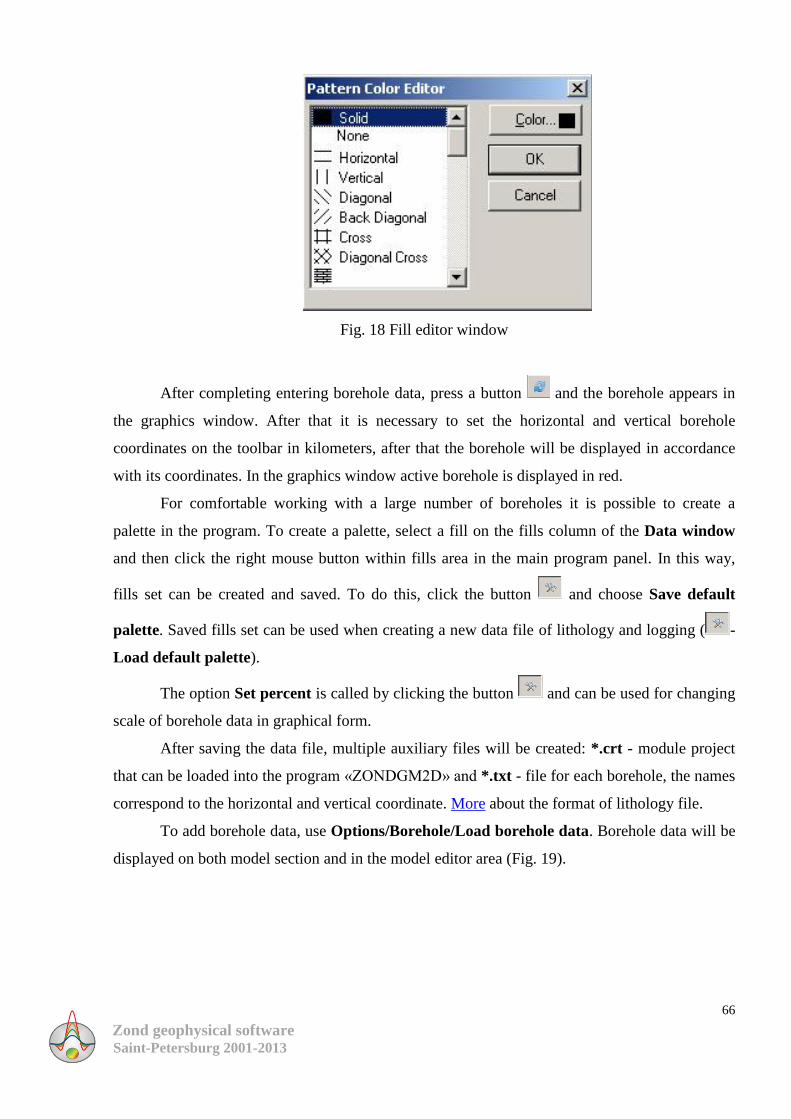
Zond geophysical software Saint-Petersburg 2001-2013
66
Fig. 18 Fill editor window
After completing entering borehole data, press a button and the borehole appears in
the graphics window. After that it is necessary to set the horizontal and vertical borehole
coordinates on the toolbar in kilometers, after that the borehole will be displayed in accordance
with its coordinates. In the graphics window active borehole is displayed in red.
For comfortable working with a large number of boreholes it is possible to create a
palette in the program. To create a palette, select a fill on the fills column of the Data window
and then click the right mouse button within fills area in the main program panel. In this way,
fills set can be created and saved. To do this, click the button and choose Save default
palette. Saved fills set can be used when creating a new data file of lithology and logging ( -
Load default palette).
The option Set percent is called by clicking the button and can be used for changing
scale of borehole data in graphical form.
After saving the data file, multiple auxiliary files will be created: *.crt - module project
that can be loaded into the program «ZONDGM2D» and *.txt - file for each borehole, the names
correspond to the horizontal and vertical coordinate. More about the format of lithology file.
To add borehole data, use Options/Borehole/Load borehole data. Borehole data will be
displayed on both model section and in the model editor area (Fig. 19).
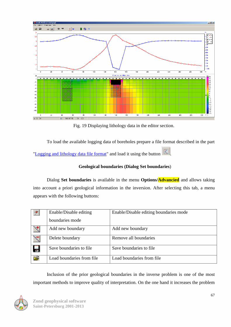
Zond geophysical software Saint-Petersburg 2001-2013
67
Fig. 19 Displaying lithology data in the editor section.
To load the available logging data of boreholes prepare a file format described in the part
"Logging and lithology data file format" and load it using the button .
Geological boundaries (Dialog Set boundaries)
Dialog Set boundaries is available in the menu Options/Advancied and allows taking
into account a priori geological information in the inversion. After selecting this tab, a menu
appears with the following buttons:
Enable/Disable editing
boundaries mode
Enable/Disable editing boundaries mode
Add new boundary Add new boundary
Delete boundary Remove all boundaries
Save boundaries to file Save boundaries to file
Load boundaries from file Load boundaries from file
Inclusion of the prior geological boundaries in the inverse problem is one of the most
important methods to improve quality of interpretation. On the one hand it increases the problem
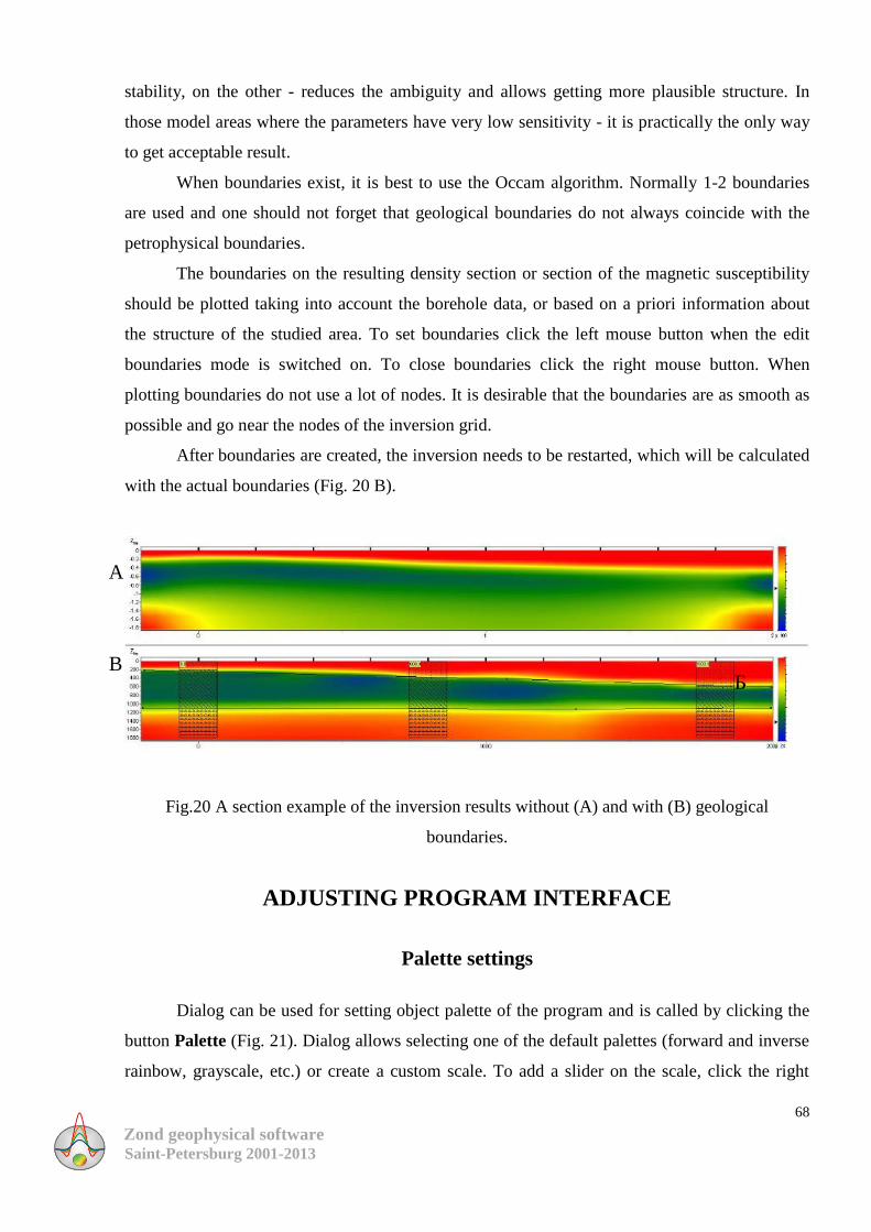
Zond geophysical software Saint-Petersburg 2001-2013
68
stability, on the other - reduces the ambiguity and allows getting more plausible structure. In
those model areas where the parameters have very low sensitivity - it is practically the only way
to get acceptable result.
When boundaries exist, it is best to use the Occam algorithm. Normally 1-2 boundaries
are used and one should not forget that geological boundaries do not always coincide with the
petrophysical boundaries.
The boundaries on the resulting density section or section of the magnetic susceptibility
should be plotted taking into account the borehole data, or based on a priori information about
the structure of the studied area. To set boundaries click the left mouse button when the edit
boundaries mode is switched on. To close boundaries click the right mouse button. When
plotting boundaries do not use a lot of nodes. It is desirable that the boundaries are as smooth as
possible and go near the nodes of the inversion grid.
After boundaries are created, the inversion needs to be restarted, which will be calculated
with the actual boundaries (Fig. 20 B).
Fig.20 A section example of the inversion results without (A) and with (B) geological
boundaries.
ADJUSTING PROGRAM INTERFACE
Palette settings
Dialog can be used for setting object palette of the program and is called by clicking the
button Palette (Fig. 21). Dialog allows selecting one of the default palettes (forward and inverse
rainbow, grayscale, etc.) or create a custom scale. To add a slider on the scale, click the right
B
A
Б
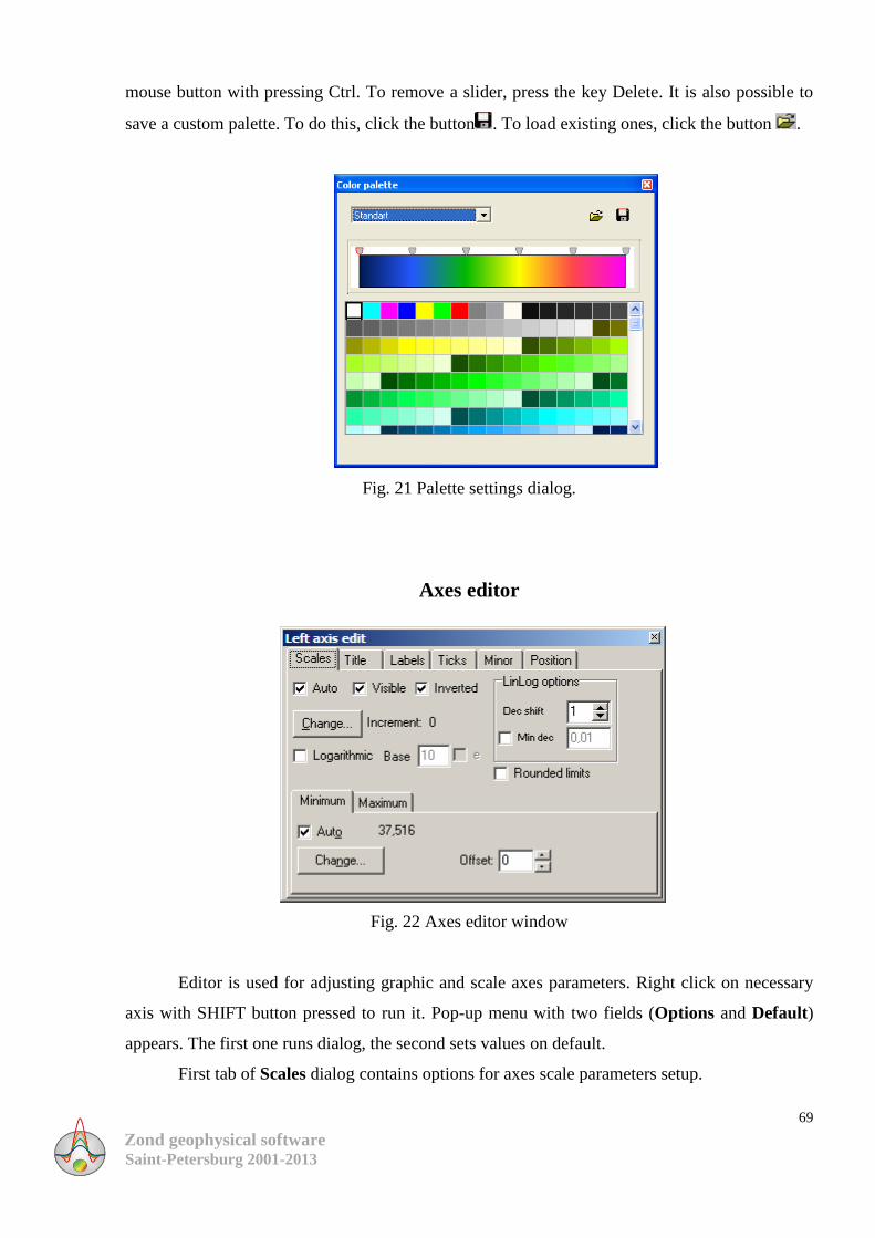
Zond geophysical software Saint-Petersburg 2001-2013
69
mouse button with pressing Ctrl. To remove a slider, press the key Delete. It is also possible to
save a custom palette. To do this, click the button . To load existing ones, click the button .
Fig. 21 Palette settings dialog.
Axes editor
Fig. 22 Axes editor window
Editor is used for adjusting graphic and scale axes parameters. Right click on necessary
axis with SHIFT button pressed to run it. Pop-up menu with two fields (Options and Default)
appears. The first one runs dialog, the second sets values on default.
First tab of Scales dialog contains options for axes scale parameters setup.
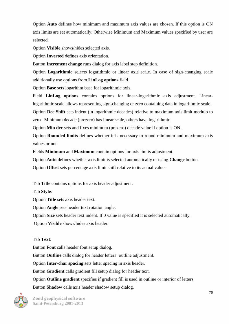
Zond geophysical software Saint-Petersburg 2001-2013
70
Option Auto defines how minimum and maximum axis values are chosen. If this option is ON
axis limits are set automatically. Otherwise Minimum and Maximum values specified by user are
selected.
Option Visible shows/hides selected axis.
Option Inverted defines axis orientation.
Button Increment change runs dialog for axis label step definition.
Option Logarithmic selects logarithmic or linear axis scale. In case of sign-changing scale
additionally use options from LinLog options field.
Option Base sets logarithm base for logarithmic axis.
Field LinLog options contains options for linear-logarithmic axis adjustment. Linear-
logarithmic scale allows representing sign-changing or zero containing data in logarithmic scale.
Option Dec Shift sets indent (in logarithmic decades) relative to maximum axis limit modulo to
zero. Minimum decade (prezero) has linear scale, others have logarithmic.
Option Min dec sets and fixes minimum (prezero) decade value if option is ON.
Option Rounded limits defines whether it is necessary to round minimum and maximum axis
values or not.
Fields Minimum and Maximum contain options for axis limits adjustment.
Option Auto defines whether axis limit is selected automatically or using Change button.
Option Offset sets percentage axis limit shift relative to its actual value.
Tab Title contains options for axis header adjustment.
Tab Style:
Option Title sets axis header text.
Option Angle sets header text rotation angle.
Option Size sets header text indent. If 0 value is specified it is selected automatically.
Option Visible shows/hides axis header.
Tab Text:
Button Font calls header font setup dialog.
Button Outline calls dialog for header letters’ outline adjustment.
Option Inter-char spacing sets letter spacing in axis header.
Button Gradient calls gradient fill setup dialog for header text.
Option Outline gradient specifies if gradient fill is used in outline or interior of letters.
Button Shadow calls axis header shadow setup dialog.
Zond geophysical software Saint-Petersburg 2001-2013
71
Tab Labels contains options for axis label adjustment.
Tab Style:
Option Visible shows/hides axes labels.
Option Multiline is used for setting multiline axes labels.
Option Round first rounds first axis label.
Option Label on axis hides labels that go beyond axis.
Option Alternate arranges labels in two lines.
Option Size sets axis label indent. If 0 value is specified it is selected automatically.
Option Angle sets label rotation angle.
Option Min separation % sets minimum percentage label spacing.
Tab Text:
Button Font calls label font setup dialog.
Button Outline calls dialog for label letters’ outline adjustment.
Option Inter-char spacing sets letter spacing in label text.
Button Gradient calls label gradient fill setup dialog.
Option Outline gradient specifies whether gradient fill is used in outline or interior of letters.
Button Shadow calls label shadow setup dialog.
Tab Title contains options for axis header adjustment.
Tab Style:
Option Title sets axis header text.
Option Angle sets header text rotation angle.
Option Size sets header text indent. If 0 value is specified it is selected automatically.
Option Visible shows/hides axis header.
Tab Text:
Button Font calls header font setup dialog.
Button Outline calls dialog for header letters’ outline adjustment.
Option Inter-char spacing sets letter spacing in axis header.
Button Gradient calls gradient fill setup dialog for header text.
Option Outline gradient specifies if gradient fill is used in outline or interior of letters.
Button Shadow calls axis header shadow setup dialog.
Zond geophysical software Saint-Petersburg 2001-2013
72
Tab Labels contains options for axis label adjustment.
Tab Style:
Option Visible shows/hides axes labels.
Option Multiline is used for setting multiline axes labels.
Option Round first rounds first axis label.
Option Label on axis hides labels that go beyond axis.
Option Alternate arranges labels in two lines.
Option Size sets axis label indent. If 0 value is specified it is selected automatically.
Option Angle sets label rotation angle.
Option Min separation % sets minimum percentage label spacing.
Tab Text:
Button Font calls label font setup dialog.
Button Outline calls dialog for label letters’ outline adjustment.
Option Inter-char spacing sets letter spacing in label text.
Button Gradient calls label gradient fill setup dialog.
Option Outline gradient specifies whether gradient fill is used in outline or interior of letters.
Button Shadow calls label shadow setup dialog.
Tab Ticks contains options for axis main ticks adjustment.
Button Axis calls axis line setup dialog.
Button Grid calls line setup dialog for main ticks’ grid.
Button Ticks calls external main axis tick setup dialog.
Option Len sets its length.
Button Inner calls internal main axis tick setup dialog.
Option Len sets its length.
Option Centered centers grid of axis ticks.
Option At labels only displays main axis ticks only if axis labels are present.
Tab Minor contains options for axis intermediate ticks adjustment.
Button Grid calls line setup dialog for intermediate ticks grid.
Button Ticks calls external intermediate axis tick line setup dialog. Option Length sets its
length.
Zond geophysical software Saint-Petersburg 2001-2013
73
Button Minor calls internal intermediate axis tick line setup dialog. Option Len sets its length
Option Count sets number of intermediate ticks between main ones.
Tab Position defines axis size and position.
Option Position % sets axis indent relative to its standard position on graph (in percent to graph
size or in screen units depending on selected option Units).
Option Start % sets axis start indent relative to its standard position on graph (in percent to
graph size).
Option End % sets axis end indent relative to its standard position on graph (in percent to graph
size).
Graph’s editor
Graphics editor is intended for graphic interface adjustment. Right click with SHIFT
button pressed on necessary graphic to run it. Pop-up menu with two fields (Options and
Default) appears. The first one runs dialog, the second sets values on default.
Tab Format contains connecting line settings.
Button Border calls connecting line parameters setup dialog.
Button Color calls color setup dialog.
Button Pattern calls pattern parameters setup dialog.
Button Outline calls graphic’s connecting line setup dialog.
Button Shadow calls shadows setup dialog.
Tab Point contains plot point settings.
Option Visible is used to show/hide plot points.
Option Style sets point shape.
Option Width sets point width in display units.
Option Height sets point height in display units.
Option Inflate margins defines if image size is zoomed in according to point size or not.
Button Pattern calls point’s color fill setup dialog.
Button Border calls point’s outline parameters setup dialog.
Button Gradient calls point’s gradient color fill setup dialog.
Tab Marks contains settings of graphic’s point marking.
Zond geophysical software Saint-Petersburg 2001-2013
74
Tab Style.
Option Visible is used to show/hide plot point marking.
Option Draw every allows plotting every second, third and so on marking depending on
selected value.
Option Angle sets point marking rotation angle.
Option Clipped defines whether point marking is plotted or not if it is located beyond
graphic borders.
Tab Arrows allows adjusting arrow from marking to point.
Button Border calls arrow line parameters setup dialog.
Button Pointer calls arrowhead shape setup dialog (options in tab Point).
Option Length sets arrow length.
Option Distance sets distance between arrowhead and plot point.
Option Arrow head sets type of arrowhead. None – arrowhead specified by Pointer
button is used. Line – classic thin arrowhead is used. Solid - classic thick arrowhead is used.
Option Size sets arrowhead size if classic arrow is used.
Tab Format contains graphic settings of marking frame.
Button Color calls frame background color selection dialog.
Button Frame calls frame line setup dialog.
Button Pattern calls background parameters setup dialog.
Option Bevel sets frame type: usual, elevated or submerged.
Option Size sets elevation or submergence level.
Option Size allows displaying rounding frame corners.
Options Transparent and Transparency sets frame seamlessness degree.
Tab Text:
Button Font calls marking font setup dialog.
Button Outline calls marking letter outline setup dialog.
Option Inter-char spacing sets letter spacing for marking text.
Button Gradient calls gradient fill for marking text setup dialog.
Option Outline gradient specifies if gradient fill is used in outline or interior of letters.
Button Shadow calls marking text shadow setup dialog.
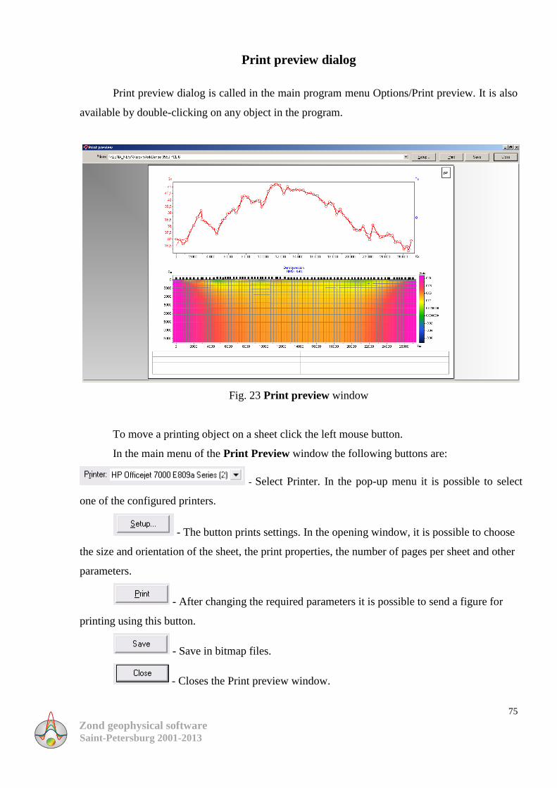
Zond geophysical software Saint-Petersburg 2001-2013
75
Print preview dialog
Print preview dialog is called in the main program menu Options/Print preview. It is also
available by double-clicking on any object in the program.
Fig. 23 Print preview window
To move a printing object on a sheet click the left mouse button.
In the main menu of the Print Preview window the following buttons are:
- Select Printer. In the pop-up menu it is possible to select
one of the configured printers.
- The button prints settings. In the opening window, it is possible to choose
the size and orientation of the sheet, the print properties, the number of pages per sheet and other
parameters.
- After changing the required parameters it is possible to send a figure for
printing using this button.
- Save in bitmap files.
- Closes the Print preview window.

Zond geophysical software Saint-Petersburg 2001-2013
76
The squares at the top of the sheet are used for making seals, stamps or company logos.
Click the right mouse button on the square and in the appeared window select a raster image to
paste. Sizes of the square can be changed with the mouse.
At the bottom of the sheet editable table is located. To add text, click the right mouse
button in the table and in the created window select required text. It is also possible to save all
the comments in the table files with clicking on the button , or to load already saved labels by
clicking on the button .
PROGRAM DATA FILE FORMAT
Data file format
Program presents universal data format which consists of information about coordinates
and relative heights of measurement points. All geometric values used by the program are set in
meters.
The data format of the program ZondGM.
The text file contains the following columns:
prpos - position of the measuring point on the profile
LATITUDE - Latitude
LONGITUDE - Longitude
z - height
GRAV - measured value of the gravity field (in mlGal)
MAG - measured values of the magnetic field (in nT)
An example of a data file:
prpos LATITUDE LONGITUDE z GRAV
479 -3.49.38.31598 -40.49.47.04385 156.645 977996.7625
478 -3.50.14.23385 -40.49.34.86847 176.749 977993.118
477 -3.50.41.81796 -40.49.12.96376 158.598 977996.16
476 -3.50.56.86075 -40.48.43.78614 153.596 977995.8746
475 -3.51.29.57703 -40.48.33.59533 163.494 977992.9616
474 -3.51.34.51079 -40.47.58.78146 150.784 977994.8251
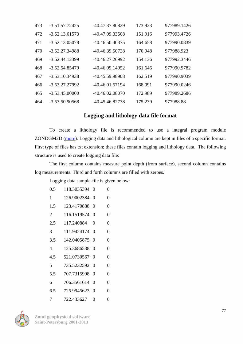
Zond geophysical software Saint-Petersburg 2001-2013
77
473 -3.51.57.72425 -40.47.37.80829 173.923 977989.1426
472 -3.52.13.61573 -40.47.09.33508 151.016 977993.4726
471 -3.52.13.05078 -40.46.50.40375 164.658 977990.0839
470 -3.52.27.34988 -40.46.39.50728 170.948 977988.923
469 -3.52.44.12399 -40.46.27.26992 154.136 977992.3446
468 -3.52.54.85479 -40.46.09.14952 161.646 977990.9782
467 -3.53.10.34938 -40.45.59.98908 162.519 977990.9039
466 -3.53.27.27992 -40.46.01.57194 168.091 977990.0246
465 -3.53.45.00000 -40.46.02.08070 172.989 977989.2686
464 -3.53.50.90568 -40.45.46.82738 175.239 977988.88
Logging and lithology data file format
To create a lithology file is recommended to use a integral program module
ZONDGM2D (more). Logging data and lithological column are kept in files of a specific format.
First type of files has txt extension; these files contain logging and lithology data. The following
structure is used to create logging data file:
The first column contains measure point depth (from surface), second column contains
log measurements. Third and forth columns are filled with zeroes.
Logging data sample-file is given below:
0.5 118.3035394 0 0
1 126.9002384 0 0
1.5 123.4170888 0 0
2 116.1519574 0 0
2.5 117.240884 0 0
3 111.9424174 0 0
3.5 142.0405875 0 0
4 125.3686538 0 0
4.5 521.0730567 0 0
5 735.5232592 0 0
5.5 707.7315998 0 0
6 706.3561614 0 0
6.5 725.9945623 0 0
7 722.433627 0 0
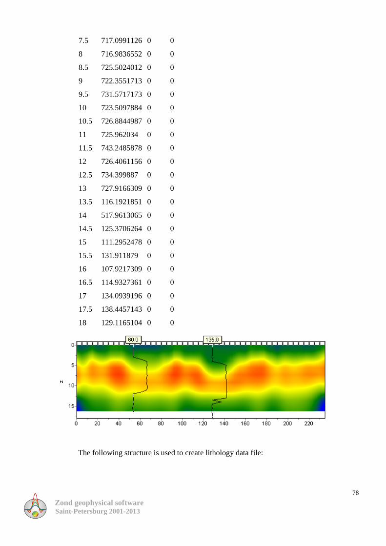
Zond geophysical software Saint-Petersburg 2001-2013
78
7.5 717.0991126 0 0
8 716.9836552 0 0
8.5 725.5024012 0 0
9 722.3551713 0 0
9.5 731.5717173 0 0
10 723.5097884 0 0
10.5 726.8844987 0 0
11 725.962034 0 0
11.5 743.2485878 0 0
12 726.4061156 0 0
12.5 734.399887 0 0
13 727.9166309 0 0
13.5 116.1921851 0 0
14 517.9613065 0 0
14.5 125.3706264 0 0
15 111.2952478 0 0
15.5 131.911879 0 0
16 107.9217309 0 0
16.5 114.9327361 0 0
17 134.0939196 0 0
17.5 138.4457143 0 0
18 129.1165104 0 0
The following structure is used to create lithology data file:
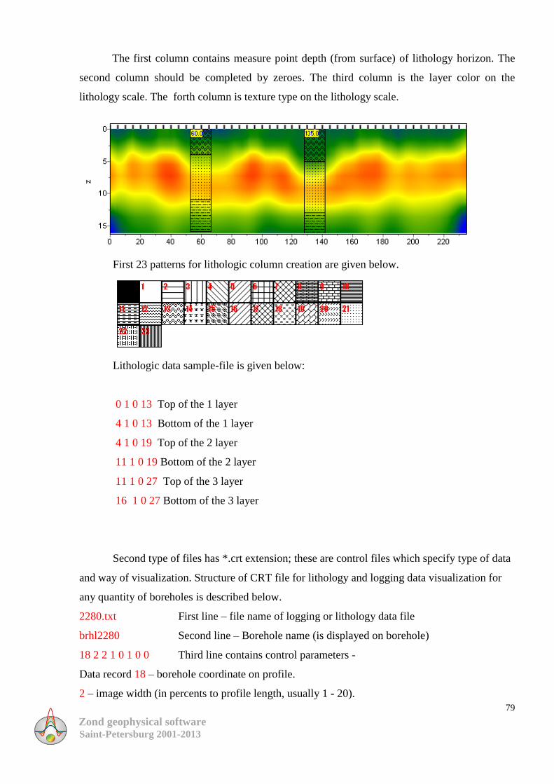
Zond geophysical software Saint-Petersburg 2001-2013
79
The first column contains measure point depth (from surface) of lithology horizon. The
second column should be completed by zeroes. The third column is the layer color on the
lithology scale. The forth column is texture type on the lithology scale.
First 23 patterns for lithologic column creation are given below.
Lithologic data sample-file is given below:
0 1 0 13 Top of the 1 layer
4 1 0 13 Bottom of the 1 layer
4 1 0 19 Top of the 2 layer
11 1 0 19 Bottom of the 2 layer
11 1 0 27 Top of the 3 layer
16 1 0 27 Bottom of the 3 layer
Second type of files has *.crt extension; these are control files which specify type of data
and way of visualization. Structure of CRT file for lithology and logging data visualization for
any quantity of boreholes is described below.
2280.txt First line – file name of logging or lithology data file
brhl2280 Second line – Borehole name (is displayed on borehole)
18 2 2 1 0 1 0 0 Third line contains control parameters -
Data record 18 – borehole coordinate on profile.
2 – image width (in percents to profile length, usually 1 - 20).
Zond geophysical software Saint-Petersburg 2001-2013
80
2 – type of data visualization 0 - 3.
0 - logging data (as graph);
1 - logging data (interpolated color column), section color scale is used for visualization;
2 - lithologic column;
3 - logging data (color column), colors for data visualization correspond to model color scale,
column colors are selected in compliance with model color scale;
1 – Logging data normalization parameter 0 - 2.
0,1 – the same minimum and maximum is used for all data;
1,2 - subtract average value from every borehole log;
0 - Logging method index (if different logging methods are displayed indices of all methods
should be specified)
0 – n-1, where n – number of methods.
1 – Plot color.
0 – Data scale is logarithmic 0 or linear 1.
0 – Vertical borehole shift relative to the earth’s surface.
3246.txt Description of the following borehole on profile
brhl3246
102 2 2 1 0 1 0 0