
© 2003 by Munehiro Nakazato. All rights reserved

TOWARD FLEXIBLE USER INTERACTION INCONTENT-BASED MULTIMEDIA DATA RETRIEVAL
BY
MUNEHIRO NAKAZATO
B.S., Keio University, 1995M.S., Keio University, 1997
DISSERTATION
Submitted in partial fulfillment of the requirementsfor the degree of Doctor of Philosophy in Computer Science
in the Graduate College of the University of Illinois at Urbana-Champaign, 2003
Urbana, Illinois

iii
Abstract
This thesis discusses various aspects of digital image retrieval and management. First, we discuss user
interface and visualization for digital image management. Two innovative systems are proposed.
3D
MARS
is immersive 3D display for image visualization and search systems. The user browses and
searches images in 3D virtual reality environment.
ImageGrouper
is another graphical user interface for
digital image search and organization. New concept,
Object-Oriented User Interaction
is introduced.
The system improves image retrieval and eases text annotation and organization of digital images.
Unlike the traditional user interfaces for image retrieval,
ImageGrouper
allows the user to group query
example images. To take advantage of this feature, a new algorithm for relevance feedback is proposed.
Next, this thesis discusses data structures and algorithms for high-dimensional data access. This is an
essential component of multimedia data retrieval. The results of preliminary experiments are presented.

iv
To Motoko, Father and Mother

Table of Contents
List of Figures . . . . . . . . . . . . . . . . . . . . . . . . . . . . . . . . . . . . . . . . . . . . . . . . . . . . . . xi
Chapter 1 Introduction. . . . . . . . . . . . . . . . . . . . . . . . . . . . . . . . . . . . . . . . . . . . . . .1
1.1 Motivation: The World of Digital Images . . . . . . . . . . . . . . . . . . . . . . . . . . . . . . . . . . . . . 1
1.2 Related Work . . . . . . . . . . . . . . . . . . . . . . . . . . . . . . . . . . . . . . . . . . . . . . . . . . . . . . . . . . . 2
1.3 Drawbacks of the Traditional Systems . . . . . . . . . . . . . . . . . . . . . . . . . . . . . . . . . . . . . . . . 3
1.3.1 User Interfaces Support for Content-based Image Retrieval . . . . . . . . . . . . . . . . . . . . . 3
1.3.2 Two-class Classification . . . . . . . . . . . . . . . . . . . . . . . . . . . . . . . . . . . . . . . . . . . . . . . . 3
1.3.3 Indexing Visual Features . . . . . . . . . . . . . . . . . . . . . . . . . . . . . . . . . . . . . . . . . . . . . . . . 4
1.4 System Overview . . . . . . . . . . . . . . . . . . . . . . . . . . . . . . . . . . . . . . . . . . . . . . . . . . . . . . . . 4
1.5 Organization of the Thesis . . . . . . . . . . . . . . . . . . . . . . . . . . . . . . . . . . . . . . . . . . . . . . . . . 5
Chapter 2 Navigation in Immersive 3D Image Space. . . . . . . . . . . . . . . . . . . . . . . .6
2.1 Introduction. . . . . . . . . . . . . . . . . . . . . . . . . . . . . . . . . . . . . . . . . . . . . . . . . . . . . . . . . . . . 6
2.2 Text Visualization vs. Image Visualization . . . . . . . . . . . . . . . . . . . . . . . . . . . . . . . . . . . . . 8
2.3 Related Work . . . . . . . . . . . . . . . . . . . . . . . . . . . . . . . . . . . . . . . . . . . . . . . . . . . . . . . . . . . 9
2.4 3D MARS: the Interactive Visualization for CBIR . . . . . . . . . . . . . . . . . . . . . . . . . . . . . . 10
2.5 User Navigation . . . . . . . . . . . . . . . . . . . . . . . . . . . . . . . . . . . . . . . . . . . . . . . . . . . . . . . . 11
2.6 System Overview . . . . . . . . . . . . . . . . . . . . . . . . . . . . . . . . . . . . . . . . . . . . . . . . . . . . . . . 17
2.7 Query Server . . . . . . . . . . . . . . . . . . . . . . . . . . . . . . . . . . . . . . . . . . . . . . . . . . . . . . . . . . 17
v

2.7.1 Total Ranking vs. Feature Ranking . . . . . . . . . . . . . . . . . . . . . . . . . . . . . . . . . . . . . . . 18
2.7.2 Implementation . . . . . . . . . . . . . . . . . . . . . . . . . . . . . . . . . . . . . . . . . . . . . . . . . . . . . 19
2.8 Visualization Engine. . . . . . . . . . . . . . . . . . . . . . . . . . . . . . . . . . . . . . . . . . . . . . . . . . . . . 20
2.8.1 Projection Strategies . . . . . . . . . . . . . . . . . . . . . . . . . . . . . . . . . . . . . . . . . . . . . . . . . . 20
2.8.1.1 Static Axes . . . . . . . . . . . . . . . . . . . . . . . . . . . . . . . . . . . . . . . . . . . . . . . . . . . . . . . 21
2.8.1.2 Dynamic Axes . . . . . . . . . . . . . . . . . . . . . . . . . . . . . . . . . . . . . . . . . . . . . . . . . . . . 21
2.9 Conclusion. . . . . . . . . . . . . . . . . . . . . . . . . . . . . . . . . . . . . . . . . . . . . . . . . . . . . . . . . . . . 22
2.10 Possible Improvement . . . . . . . . . . . . . . . . . . . . . . . . . . . . . . . . . . . . . . . . . . . . . . . . . . 22
2.10.1 Integration of Browsing and Searching . . . . . . . . . . . . . . . . . . . . . . . . . . . . . . . . . . . 23
2.10.2 Migrating to 6-Sided CAVE . . . . . . . . . . . . . . . . . . . . . . . . . . . . . . . . . . . . . . . . . . . 23
2.10.3 Improvement on User Input Methods . . . . . . . . . . . . . . . . . . . . . . . . . . . . . . . . . . . 24
2.10.4 Improvement on Navigation. . . . . . . . . . . . . . . . . . . . . . . . . . . . . . . . . . . . . . . . . . . 24
2.10.5 Multi-Cluster Display . . . . . . . . . . . . . . . . . . . . . . . . . . . . . . . . . . . . . . . . . . . . . . . . 25
Chapter 3 Group-Oriented User Interface for Digital Image Retrieval and Management . . . . . . . . . . . . . . . . . . . . . . . . . . . . . . . . . . . . . . . . . . . . . . . . . . . . . . .26
3.1 User Interface Support for Content-based Image Retrieval . . . . . . . . . . . . . . . . . . . . . . . . 26
3.2 Related Work . . . . . . . . . . . . . . . . . . . . . . . . . . . . . . . . . . . . . . . . . . . . . . . . . . . . . . . . . . 27
3.2.1 The Traditional Approaches: Incremental Query . . . . . . . . . . . . . . . . . . . . . . . . . . . . 27
3.2.2 Limitation of Incremental Query . . . . . . . . . . . . . . . . . . . . . . . . . . . . . . . . . . . . . . . . 30
3.2.3 El Ninõ System. . . . . . . . . . . . . . . . . . . . . . . . . . . . . . . . . . . . . . . . . . . . . . . . . . . . . . 32
3.3 Query-by-Groups with ImageGrouper . . . . . . . . . . . . . . . . . . . . . . . . . . . . . . . . . . . . . . . 32
3.3.1 The Basic Query Sequences . . . . . . . . . . . . . . . . . . . . . . . . . . . . . . . . . . . . . . . . . . . . 34
3.4 The Flexibility of Query-by-Groups . . . . . . . . . . . . . . . . . . . . . . . . . . . . . . . . . . . . . . . . . 37
3.4.1 Trial and Error Query by Mouse Dragging . . . . . . . . . . . . . . . . . . . . . . . . . . . . . . . . . 37
vi

3.4.2 Groups in a Group . . . . . . . . . . . . . . . . . . . . . . . . . . . . . . . . . . . . . . . . . . . . . . . . . . . 37
3.5 Experiment on Trial and Error Query . . . . . . . . . . . . . . . . . . . . . . . . . . . . . . . . . . . . . . . 38
3.6 Text Annotations on Images. . . . . . . . . . . . . . . . . . . . . . . . . . . . . . . . . . . . . . . . . . . . . . . 41
3.6.1 Current Approaches for Text Annotation . . . . . . . . . . . . . . . . . . . . . . . . . . . . . . . . . . 41
3.6.2 Annotation by Groups . . . . . . . . . . . . . . . . . . . . . . . . . . . . . . . . . . . . . . . . . . . . . . . . 42
3.6.2.1 Annotating New Images with the Same Keywords. . . . . . . . . . . . . . . . . . . . . . . . . 42
3.6.2.2 Hierarchical Annotation with Groups in a Group . . . . . . . . . . . . . . . . . . . . . . . . . 43
3.6.2.3 Overlap between Images . . . . . . . . . . . . . . . . . . . . . . . . . . . . . . . . . . . . . . . . . . . . 43
3.7 Organizing Images by Groups . . . . . . . . . . . . . . . . . . . . . . . . . . . . . . . . . . . . . . . . . . . . . 44
3.7.1 Photo Albums and Group Icons . . . . . . . . . . . . . . . . . . . . . . . . . . . . . . . . . . . . . . . . . 44
3.8 Usability Study. . . . . . . . . . . . . . . . . . . . . . . . . . . . . . . . . . . . . . . . . . . . . . . . . . . . . . . . . 47
3.8.1 Experimental Settings . . . . . . . . . . . . . . . . . . . . . . . . . . . . . . . . . . . . . . . . . . . . . . . . . 47
3.8.1.1 Subjects . . . . . . . . . . . . . . . . . . . . . . . . . . . . . . . . . . . . . . . . . . . . . . . . . . . . . . . . . 47
3.8.1.2 Apparatus . . . . . . . . . . . . . . . . . . . . . . . . . . . . . . . . . . . . . . . . . . . . . . . . . . . . . . . 48
3.8.2 Scenarios. . . . . . . . . . . . . . . . . . . . . . . . . . . . . . . . . . . . . . . . . . . . . . . . . . . . . . . . . . . 48
3.8.2.1 Experimental Task. . . . . . . . . . . . . . . . . . . . . . . . . . . . . . . . . . . . . . . . . . . . . . . . . 48
3.8.2.2 Training Session . . . . . . . . . . . . . . . . . . . . . . . . . . . . . . . . . . . . . . . . . . . . . . . . . . 49
3.8.2.3 Experiment Session . . . . . . . . . . . . . . . . . . . . . . . . . . . . . . . . . . . . . . . . . . . . . . . . 49
3.8.3 The Results . . . . . . . . . . . . . . . . . . . . . . . . . . . . . . . . . . . . . . . . . . . . . . . . . . . . . . . . . 50
3.8.3.1 Error Rate . . . . . . . . . . . . . . . . . . . . . . . . . . . . . . . . . . . . . . . . . . . . . . . . . . . . . . . 50
3.8.3.2 Task Completion Time . . . . . . . . . . . . . . . . . . . . . . . . . . . . . . . . . . . . . . . . . . . . . 51
3.8.4 Improving ImageGrouper Based on the Lessons We Learned . . . . . . . . . . . . . . . . . . . 53
3.9 Implementation Detail . . . . . . . . . . . . . . . . . . . . . . . . . . . . . . . . . . . . . . . . . . . . . . . . . . . 54
vii

3.9.1 The Client-Server Architecture . . . . . . . . . . . . . . . . . . . . . . . . . . . . . . . . . . . . . . . . . . 54
3.9.1.1 The User Interface Client . . . . . . . . . . . . . . . . . . . . . . . . . . . . . . . . . . . . . . . . . . . 54
3.9.1.2 The Query Server . . . . . . . . . . . . . . . . . . . . . . . . . . . . . . . . . . . . . . . . . . . . . . . . . 55
3.9.2 Relevance Feedback Algorithm in the Query Engine. . . . . . . . . . . . . . . . . . . . . . . . . . 55
3.10 Conclusion and Future Work. . . . . . . . . . . . . . . . . . . . . . . . . . . . . . . . . . . . . . . . . . . . . 56
Chapter 4 Relevance Feedback Algorithms for Group Query . . . . . . . . . . . . . . .59
4.1 Introduction. . . . . . . . . . . . . . . . . . . . . . . . . . . . . . . . . . . . . . . . . . . . . . . . . . . . . . . . . . . 59
4.2 Related Work . . . . . . . . . . . . . . . . . . . . . . . . . . . . . . . . . . . . . . . . . . . . . . . . . . . . . . . . . . 60
4.2.1 Image Retrieval as a One-Class Problem . . . . . . . . . . . . . . . . . . . . . . . . . . . . . . . . . . . 61
4.2.2 Image Retrieval as a Two-Class Problem. . . . . . . . . . . . . . . . . . . . . . . . . . . . . . . . . . . 63
4.2.3 Image Retrieval as a (1+x)-Class Problem . . . . . . . . . . . . . . . . . . . . . . . . . . . . . . . . . . 64
4.2.4 Multi-Class Relevance Feedback . . . . . . . . . . . . . . . . . . . . . . . . . . . . . . . . . . . . . . . . . 65
4.3 Proposed Approach: Extending to a (x+y)-Class Problem . . . . . . . . . . . . . . . . . . . . . . . . . 68
4.4 Implementation . . . . . . . . . . . . . . . . . . . . . . . . . . . . . . . . . . . . . . . . . . . . . . . . . . . . . . . . 70
4.5 Analysis on Toy Problems . . . . . . . . . . . . . . . . . . . . . . . . . . . . . . . . . . . . . . . . . . . . . . . . 71
4.6 Experiments on Real Data . . . . . . . . . . . . . . . . . . . . . . . . . . . . . . . . . . . . . . . . . . . . . . . . 72
4.6.1 Data Sets. . . . . . . . . . . . . . . . . . . . . . . . . . . . . . . . . . . . . . . . . . . . . . . . . . . . . . . . . . . 72
4.6.2 Performance Measures . . . . . . . . . . . . . . . . . . . . . . . . . . . . . . . . . . . . . . . . . . . . . . . . 75
4.6.3 Ranking Strategies for GBDA . . . . . . . . . . . . . . . . . . . . . . . . . . . . . . . . . . . . . . . . . . . 75
4.6.4 Results . . . . . . . . . . . . . . . . . . . . . . . . . . . . . . . . . . . . . . . . . . . . . . . . . . . . . . . . . . . . 77
4.7 Conclusion. . . . . . . . . . . . . . . . . . . . . . . . . . . . . . . . . . . . . . . . . . . . . . . . . . . . . . . . . . . . 80
4.8 Possible Improvement . . . . . . . . . . . . . . . . . . . . . . . . . . . . . . . . . . . . . . . . . . . . . . . . . . . 80
4.8.1 Groups with Different Sizes . . . . . . . . . . . . . . . . . . . . . . . . . . . . . . . . . . . . . . . . . . . . 80
viii

4.8.2 Automated Clustering of Groups . . . . . . . . . . . . . . . . . . . . . . . . . . . . . . . . . . . . . . . . 81
4.8.3 More than Two Groups . . . . . . . . . . . . . . . . . . . . . . . . . . . . . . . . . . . . . . . . . . . . . . . 81
Chapter 5 Integrating ImageGrouper into the 3D Virtual Space . . . . . . . . . . . . . .82
5.1 Introduction. . . . . . . . . . . . . . . . . . . . . . . . . . . . . . . . . . . . . . . . . . . . . . . . . . . . . . . . . . . 82
5.2 Design Choices. . . . . . . . . . . . . . . . . . . . . . . . . . . . . . . . . . . . . . . . . . . . . . . . . . . . . . . . . 84
5.3 User Interaction of Grouper in 3D MARS . . . . . . . . . . . . . . . . . . . . . . . . . . . . . . . . . . . . 84
5.4 System Architecture . . . . . . . . . . . . . . . . . . . . . . . . . . . . . . . . . . . . . . . . . . . . . . . . . . . . . 86
5.5 The Benefits of Integration. . . . . . . . . . . . . . . . . . . . . . . . . . . . . . . . . . . . . . . . . . . . . . . . 87
Chapter 6 Storage and Visual Features for Content-based Image Retrieval . . . . .89
6.1 Data Structure for High-Dimensional Data Access. . . . . . . . . . . . . . . . . . . . . . . . . . . . . . 89
6.1.1 Background. . . . . . . . . . . . . . . . . . . . . . . . . . . . . . . . . . . . . . . . . . . . . . . . . . . . . . . . . 89
6.2 Preliminary Experiments . . . . . . . . . . . . . . . . . . . . . . . . . . . . . . . . . . . . . . . . . . . . . . . . . 91
6.3 Image Retrieval by Local Image Features . . . . . . . . . . . . . . . . . . . . . . . . . . . . . . . . . . . . . 92
6.4 Integration of Content-based and Keyword-based Image Retrieval . . . . . . . . . . . . . . . . . . 94
Bibliography . . . . . . . . . . . . . . . . . . . . . . . . . . . . . . . . . . . . . . . . . . . . . . . . . . . . . . .97
Appendix A Image Features in the Systems . . . . . . . . . . . . . . . . . . . . . . . . . . . . .106
A.1 Color Distribution. . . . . . . . . . . . . . . . . . . . . . . . . . . . . . . . . . . . . . . . . . . . . . . . . . . . . 106
A.2 Texture . . . . . . . . . . . . . . . . . . . . . . . . . . . . . . . . . . . . . . . . . . . . . . . . . . . . . . . . . . . . . 108
A.3 Edge Structures . . . . . . . . . . . . . . . . . . . . . . . . . . . . . . . . . . . . . . . . . . . . . . . . . . . . . . . 108
Appendix B Implementation Details of ImageGrouper and Query Engine . . . . .110
B.1 ImageGrouper . . . . . . . . . . . . . . . . . . . . . . . . . . . . . . . . . . . . . . . . . . . . . . . . . . . . . . . . 110
B.1.1 Structure of ImageGrouper User Interface . . . . . . . . . . . . . . . . . . . . . . . . . . . . . . . . 110
B.1.2 Image Drag Operation . . . . . . . . . . . . . . . . . . . . . . . . . . . . . . . . . . . . . . . . . . . . . . . 111
ix

B.2 Query Engine . . . . . . . . . . . . . . . . . . . . . . . . . . . . . . . . . . . . . . . . . . . . . . . . . . . . . . . . 113
B.2.1 Overview of the Query Engine . . . . . . . . . . . . . . . . . . . . . . . . . . . . . . . . . . . . . . . . . 113
B.2.2 System Configurations . . . . . . . . . . . . . . . . . . . . . . . . . . . . . . . . . . . . . . . . . . . . . . . 115
B.2.3 Client-Server Configuration . . . . . . . . . . . . . . . . . . . . . . . . . . . . . . . . . . . . . . . . . . . 115
B.2.3.1 Standalone Configuration . . . . . . . . . . . . . . . . . . . . . . . . . . . . . . . . . . . . . . . . . . 117
B.3 Building Instructions . . . . . . . . . . . . . . . . . . . . . . . . . . . . . . . . . . . . . . . . . . . . . . . . . . . 117
B.3.1 Directory Structure. . . . . . . . . . . . . . . . . . . . . . . . . . . . . . . . . . . . . . . . . . . . . . . . . . 117
B.3.2 Building Systems . . . . . . . . . . . . . . . . . . . . . . . . . . . . . . . . . . . . . . . . . . . . . . . . . . . 118
B.3.2.1 Additional Libraries. . . . . . . . . . . . . . . . . . . . . . . . . . . . . . . . . . . . . . . . . . . . . . . 118
B.3.2.2 Setting Java Parameter. . . . . . . . . . . . . . . . . . . . . . . . . . . . . . . . . . . . . . . . . . . . . 119
B.3.2.3 Modifying Server Makefile . . . . . . . . . . . . . . . . . . . . . . . . . . . . . . . . . . . . . . . . . 119
B.3.2.4 Compiling. . . . . . . . . . . . . . . . . . . . . . . . . . . . . . . . . . . . . . . . . . . . . . . . . . . . . . 120
B.3.3 Running Systems . . . . . . . . . . . . . . . . . . . . . . . . . . . . . . . . . . . . . . . . . . . . . . . . . . . 120
B.3.3.1 Image File Location. . . . . . . . . . . . . . . . . . . . . . . . . . . . . . . . . . . . . . . . . . . . . . . 120
B.3.3.2 Metadata File Location . . . . . . . . . . . . . . . . . . . . . . . . . . . . . . . . . . . . . . . . . . . . 120
B.3.3.3 Server URL . . . . . . . . . . . . . . . . . . . . . . . . . . . . . . . . . . . . . . . . . . . . . . . . . . . . . 120
B.3.3.4 Starting Systems . . . . . . . . . . . . . . . . . . . . . . . . . . . . . . . . . . . . . . . . . . . . . . . . . 121
Vita . . . . . . . . . . . . . . . . . . . . . . . . . . . . . . . . . . . . . . . . . . . . . . . . . . . . . . . . . . . . .122
x

List of Figures
Chapter 1 Introduction. . . . . . . . . . . . . . . . . . . . . . . . . . . . . . . . . . . . . . . . . . . . . 1
1-1 The Digital Image Toolkit.. . . . . . . . . . . . . . . . . . . . . . . . . . . . . . . . . . . . . . . . . . . . . . . 5
Chapter 2 Navigation in Immersive 3D Image Space. . . . . . . . . . . . . . . . . . . . . . 6
2-1 Initial configuration of 3DMARS. . . . . . . . . . . . . . . . . . . . . . . . . . . . . . . . . . . . . . . . . 13
2-2 3D MARS in CAVE . . . . . . . . . . . . . . . . . . . . . . . . . . . . . . . . . . . . . . . . . . . . . . . . . . 14
2-3 3D MARS on a desktop VR . . . . . . . . . . . . . . . . . . . . . . . . . . . . . . . . . . . . . . . . . . . . 14
2-4 The result after the user selected one “red flower” picture (in Fixed axes mode.) The queryexample is displayed near the origin. . . . . . . . . . . . . . . . . . . . . . . . . . . . . . . . . . . . . . . 15
2-5 The result after the user selected another “flower” images. Red flowers of different textureare aligned along the red arrow. . . . . . . . . . . . . . . . . . . . . . . . . . . . . . . . . . . . . . . . . . . 15
2-6 The Sphere Mode. The number of images is 100. . . . . . . . . . . . . . . . . . . . . . . . . . . . . 16
2-7 The sphere mode from a different view angle (from the zenith of the space.) Relationshipbetween color and structure is visualized . . . . . . . . . . . . . . . . . . . . . . . . . . . . . . . . . . . 16
2-8 The system architecture of 3D MARS . . . . . . . . . . . . . . . . . . . . . . . . . . . . . . . . . . . . . 17
Chapter 3 Group-Oriented User Interface for Digital Image Retrieval and Management . . . . . . . . . . . . . . . . . . . . . . . . . . . . . . . . . . . . . . . . . . . . . . . . . . . . . 26
3-2 Example of “More is not necessarily better”. The left is the case of one example, the rightis the case of two examples. . . . . . . . . . . . . . . . . . . . . . . . . . . . . . . . . . . . . . . . . . . . . . 28
3-1 Typical Graphical User Interfaces for CBIR Systems: (a) Slider-based GUI, (b) Click-based GUI. On both systems, the search results are also displayed on the same workspace.29
3-3 The overview of ImageGrouper user interface. . . . . . . . . . . . . . . . . . . . . . . . . . . . . . . . 33
xi

3-4 The sequence of the basic query operation on ImageGrouper . . . . . . . . . . . . . . . . . . . 36
3-5 The number of hits until the 10th round or convergence. . . . . . . . . . . . . . . . . . . . . . . 40
3-6 Groups in a group. In ImageGrouper, the user can create a hierarchy of image group. Inthis example, the entire group is “cars.” Once the whole group is annotated as “car,” theuser only need to type “red” to annotate the red cars. . . . . . . . . . . . . . . . . . . . . . . . . . . 46
3-7 Overlap between groups. Two images in the overlapped region contain both mountainand cloud. Once the two groups are annotated, the overlapped region are automaticallyannotated with both keywords. . . . . . . . . . . . . . . . . . . . . . . . . . . . . . . . . . . . . . . . . . . 46
3-8 The Usability Test Setting (Click-base GUI) . . . . . . . . . . . . . . . . . . . . . . . . . . . . . . . . 50
3-9 The average time required to select each images in different problems. The X-axis is thetotal number of images selected during in the problems. . . . . . . . . . . . . . . . . . . . . . . . 52
3-10 The average selection time per image. The differences are statistically significant at p <.001. The click-baed user interface achieves the shortest task completion time. . . . . . . 53
Chapter 4 Relevance Feedback Algorithms for Group Query . . . . . . . . . . . . . 59
4-1 Co-evolution of GUI design and search algorithm development. A new GUI designmotivates development of a new search algorithm. Meanwhile, an existing searchalgorithm could be reinforced by a new GUI. . . . . . . . . . . . . . . . . . . . . . . . . . . . . . . . 60
4-2 Graphical concepts of the previous space translation scheme. (a) Two-class problemscheme tries to divide data into two classes, which are positive and negative groups. (b)(1+x)-class scheme handles problem as one positive group and multiple negative groups.. 65
4-3 White flowers and Red flowers. Both groups can be considered as subsets of “flower class”In ImageGrouper, users can separate them into two positive groups. . . . . . . . . . . . . . . 68
4-4 Concept of the new feature space transform. It minimizes the scatter of each positive classwhile maximizing the scatter between positive and negative samples. . . . . . . . . . . . . . . 70
4-5 Comparison of MDA, BDA, and GBDA on toy problems 1. The original data (in 3D)and the result projections (2D) are plotted. In this problem, GBDA performs similar toMDA. . . . . . . . . . . . . . . . . . . . . . . . . . . . . . . . . . . . . . . . . . . . . . . . . . . . . . . . . . . . . . 73
4-6 Comparison of MDA, BDA, and GBDA on toy problems 2. The original data (in 3D)and the result projections (2D) are plotted. In this toy problem, GBDA performssimilarly to BDA.. . . . . . . . . . . . . . . . . . . . . . . . . . . . . . . . . . . . . . . . . . . . . . . . . . . . . 74
4-7 Sample Query Images. Each set is divided into two sub-sets. . . . . . . . . . . . . . . . . . . . . 76
xii
4-8 Comparison of BDA and GBDA on the real data. The results are shown in the weightedhit count. . . . . . . . . . . . . . . . . . . . . . . . . . . . . . . . . . . . . . . . . . . . . . . . . . . . . . . . . . . . 78
4-9 Comparison of BDA and GBDA on the real data (measured in the precision and recallfor different sample size) . . . . . . . . . . . . . . . . . . . . . . . . . . . . . . . . . . . . . . . . . . . . . . . 79
Chapter 5 Integrating ImageGrouper into the 3D Virtual Space. . . . . . . . . . . . 82
5-1 User interacting in 3DMARS with a wireless-equipped note book PC. . . . . . . . . . . . . 85
5-2 Overview of the integrated system . . . . . . . . . . . . . . . . . . . . . . . . . . . . . . . . . . . . . . . . 87
Chapter 6 Storage and Visual Features for Content-based Image Retrieval. . . 89
6-1 Comparison of K-Nearest neighbor search time. K=50, Dimemsion=37, The number oforiginal data is 100,000 (28MB.) Iterated 100,000 times. . . . . . . . . . . . . . . . . . . . . . . 92
6-2 Block based image selection. In this example, the image is divided into 5 x 5 blocks. Theuser may be interested in region of 2 x 2 colored blue. . . . . . . . . . . . . . . . . . . . . . . . . . 93
6-3 Approximating image region from smaller blocks. . . . . . . . . . . . . . . . . . . . . . . . . . . . . 94
6-4 Quad-Tree Decomposition [98]. . . . . . . . . . . . . . . . . . . . . . . . . . . . . . . . . . . . . . . . . . 95
6-5 Example of Keyword and Free Text Annotation of MPEG-7 . . . . . . . . . . . . . . . . . . . . 95
Appendix A Image Features in the Systems . . . . . . . . . . . . . . . . . . . . . . . . . . . 106
A-1 The HSV color space. . . . . . . . . . . . . . . . . . . . . . . . . . . . . . . . . . . . . . . . . . . . . . . . . 107
A-2 The wavelet texture features . . . . . . . . . . . . . . . . . . . . . . . . . . . . . . . . . . . . . . . . . . . . 108
Appendix B Implementation Details of ImageGrouper and Query Engine . . . 110
B-1 Layered structure of ImageGrouper user interface . . . . . . . . . . . . . . . . . . . . . . . . . . . 112
B-2 Image Dragging from the Grid to the Palette. . . . . . . . . . . . . . . . . . . . . . . . . . . . . . . 113
B-3 Client-Server configuration.. . . . . . . . . . . . . . . . . . . . . . . . . . . . . . . . . . . . . . . . . . . . 116
B-4 Standalone configuration with a local query engine . . . . . . . . . . . . . . . . . . . . . . . . . . 117
xiii
Chapter 1
Introduction
1.1 Motivation: The World of Digital ImagesMore and more people are enjoying Digital Imaging these days [37][64]. New inexpensive and high
quality digital cameras hit the market every month. They are replacing traditional film cameras. Even
camera-equipped mobile phones have appeared [93]. We can take plenty of digital pictures without
worrying about the cost of films. We can easily edit pictures, as we like. We can share the images with
our family or friends by E-mail and World-Wide Web.
Meanwhile, hospitals store a huge amount of medical images such as MRT and CT in digital formats.
Digital museums are becoming numerous, too. Thus, Digital Imaging has important roles both in
consumer and professional markets.
The users are, however, having difficulty in organizing and searching a large number of images in the
databases. The current commercial database systems are designed for text data and not suitable for Data
Mining [39] of digital images. To make matters worse, digital image systems often automatically
generate file names like “DSCF0052.JPG,” which are meaningless to humans. An Efficient way for
digital image management is desired.
1
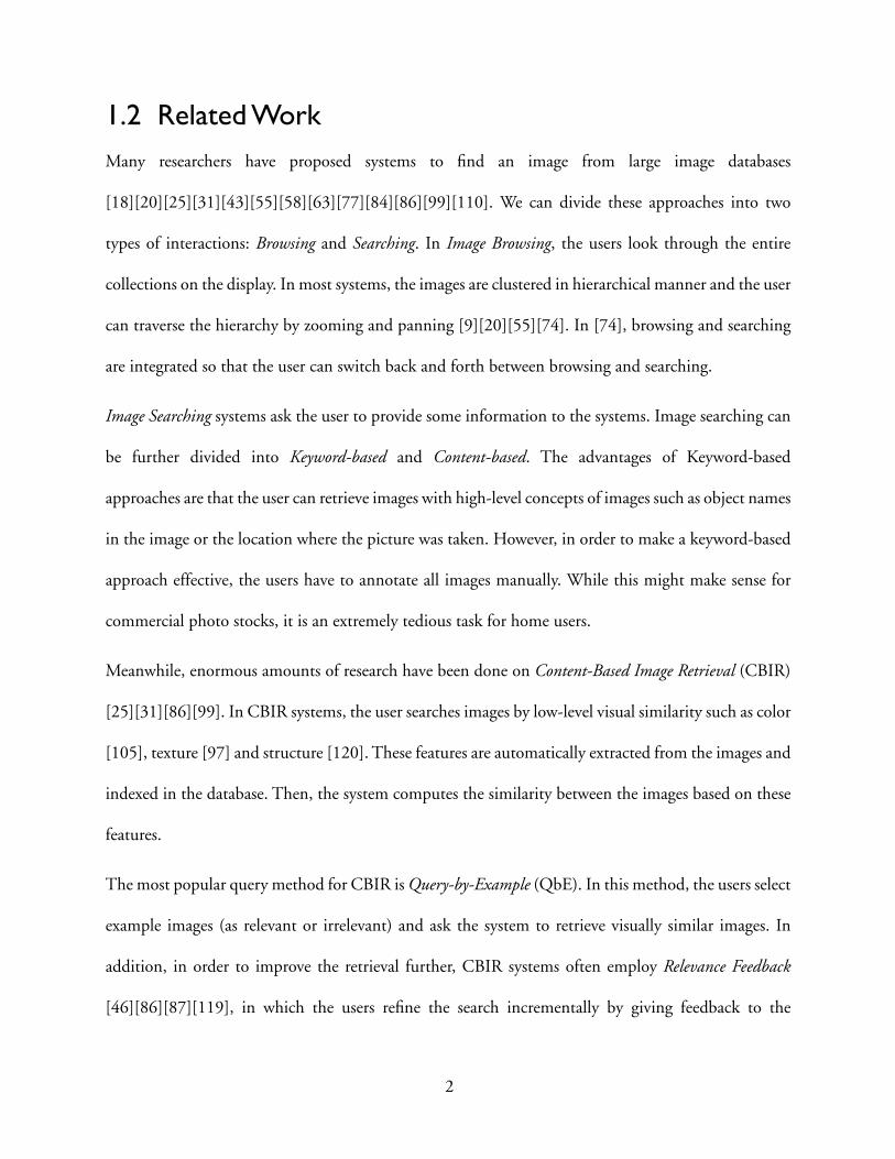
1.2 Related WorkMany researchers have proposed systems to find an image from large image databases
[18][20][25][31][43][55][58][63][77][84][86][99][110]. We can divide these approaches into two
types of interactions: Browsing and Searching. In Image Browsing, the users look through the entire
collections on the display. In most systems, the images are clustered in hierarchical manner and the user
can traverse the hierarchy by zooming and panning [9][20][55][74]. In [74], browsing and searching
are integrated so that the user can switch back and forth between browsing and searching.
Image Searching systems ask the user to provide some information to the systems. Image searching can
be further divided into Keyword-based and Content-based. The advantages of Keyword-based
approaches are that the user can retrieve images with high-level concepts of images such as object names
in the image or the location where the picture was taken. However, in order to make a keyword-based
approach effective, the users have to annotate all images manually. While this might make sense for
commercial photo stocks, it is an extremely tedious task for home users.
Meanwhile, enormous amounts of research have been done on Content-Based Image Retrieval (CBIR)
[25][31][86][99]. In CBIR systems, the user searches images by low-level visual similarity such as color
[105], texture [97] and structure [120]. These features are automatically extracted from the images and
indexed in the database. Then, the system computes the similarity between the images based on these
features.
The most popular query method for CBIR is Query-by-Example (QbE). In this method, the users select
example images (as relevant or irrelevant) and ask the system to retrieve visually similar images. In
addition, in order to improve the retrieval further, CBIR systems often employ Relevance Feedback
[46][86][87][119], in which the users refine the search incrementally by giving feedback to the
2
previous query result. In Active Learning Relevance Feedback [110], the users are asked to select relevant
images from a set of the most informative images.
1.3 Drawbacks of the Traditional SystemsIn this section, we briefly discuss the major drawbacks of traditional CBIR systems in several aspects.
1.3.1 User Interfaces Support for Content-based Image Retrieval
In most user interfaces for digital image retrieval, the query results are aligned in a grid. This means the
results must be ordered and mapped in a line. However, the visual features of CBIR systems are made
of high-dimensional numerical data. Therefore, much information has to be discarded for the result
display. Next, in CBIR systems, there are inevitable gaps between low-level image features and the user’s
concepts. Therefore, trying different combinations of query examples in query-by-example is essential
for successful retrieval. Most systems do not support this type of query, though. These problems are
addressed in Chapter 2 and Chapter 3.
1.3.2 Two-class Classification
Most CBIR systems ask the user to specify relevant and irrelevant image examples. Therefore, many
relevance feedback algorithms for CBIR addressed image retrieval as a two-class pattern classification
problem that classifies data into two classes (positive and negative) [26][48][86][87][110][117][118].
These approaches, however, introduce undesirable side effects because they mix up all negative
examples into one class. In the actual scenario of image retrieval, negative examples can be from many
classes of images in the database.
3

In addition, the user’s high-level concepts often cannot be expressed by only one class of images. Our
new flexible user interface allows the user to specify more than one group of relevant images. Not many
researchers have addressed multi-positive class relevance feedback algorithms [76]. We will discuss how
we extend two-class classification to take advantages of multiple positive classes in Chapter 4.
1.3.3 Indexing Visual Features
The visual image features for CBIR systems are high-dimensional numerical data. It is difficult to
manage these data with traditional commercial database systems because these systems are designed for
text data and low-dimensional numerical data. While many researchers have proposed architectures for
indexing high-dimensional data [10][11][12][35] [38][50][57][81][88][113][114], these systems are
not tested in real world performance. Often, a simpler method can outperform those sophisticated
systems. Section 6.1 discusses this problem in detail.
1.4 System OverviewFigure 1-1 shows the overview of our proposed system. The system consists of several components as
follows.
• User Interface (Chapter 2, Chapter 3 and Chapter 5)
• Query Engine (Chapter 4)
• Fast Data Indexing Structure (Section 6.1 in Chapter 6)
• Feature Extraction (Section 6.3 in Chapter 6)
• Meta-data Management (Section 6.4 in Chapter 6)
We discuss each component in the following chapters.
4

1.5 Organization of the ThesisIn the next chapter, we propose an innovative 3D visualization system for digital image named 3D
MARS. 3D MARS allows the user to browse and search images in an immersive virtual reality
environment. In Chapter 3, a new graphical user interface (GUI) for digital image retrieval and
organization is presented. The new GUI, named ImageGrouper introduces a new interaction method
for content-based image query. To take advantages of this new interaction method, a new algorithm
for relevance feedback is proposed in Chapter 4. In Chapter 5, 3D MARS and ImageGrouper are
integrated to provide more flexible image query. Finally, several other research topics are discussed in
Chapter 6.
Meta Data Manager
Image Files Database
Keyword Annotation
Retrieval
Query
KeywordsLow Level
Image Features
Query Engine Fast Index
Face Features
User Interfaces
Feature Extraction
Figure 1-1. The Digital Image Toolkit.
5
Chapter 2
Navigation in Immersive 3D Image Space
In this chapter, we propose an interactive 3D visualization system for Content-based Image Retrieval
(CBIR) named 3D MARS. In 3D MARS, query results are displayed on a projection-based immersive
Virtual Reality system or a desktop Virtual Reality system. Based on the users’ feedback, the system
dynamically reorganizes its visualization strategies. 3D MARS eases tedious task of searching images
from a large set of images. In addition, the sphere display mode effectively visualize clusters in the
image database. This will be a powerful analyzing tool for CBIR researchers.
2.1 IntroductionWhile CBIR systems provided us with a smart way of searching images, they had a significant
limitation. First, the image features consist of high-dimensional vectors of different image properties
such as color, texture and structure. Meanwhile, in the traditional CBIR systems, the query results are
ordered and displayed in a line based on the weighted sum of the distance measures. This means high-
dimensional image features have to be mapped on one dimensional space. As a result, much
6
information can be lost for visualization. This causes problems especially when the number of query
examples is small. The system cannot tell which feature is the most important for a user. Consequently,
the most important image may not appear in the early stage of query operations. One solution to this
problem is to allow the user to adjust the query parameter as done in many image retrieval systems [31].
In this approach, the user has to specify the weights of each feature. This process, however, is very
tedious and difficult for novice users.
Second, in the conventional two-dimensional display, the query result images are tiled in a monitor.
Thus, only limited number of images can be displayed at the same time. It is painful for user to go back
and forth in the browser by clicking “Next” and “Previous” buttons.
3D visualization for Content-Based Images Retrieval (CBIR) alleviates these problems. In addition, it
eases integration of searching and browsing images in a large image database. Many researchers have
proposed 3D visualization system for CBIR. In most approaches, however, the images features for
display are fixed by the system developers. Meanwhile, not all features are always equally important for
the users. Moreover, in most systems, all images in the database are displayed despite the user’s interest.
Displaying too many images consumes the resources and may confuse the users.
In this chapter, we propose a new visualization system for Content-based image retrieval named 3D
MARS. In this system, images are displayed on a projection-based immersive Virtual Reality or non-
immersive desktop VR. The three dimensional space can display more images than traditional CBIR
systems at the same time. By giving different meaning to each axis, the user can simultaneously browse
the retrieved images with respect to three different criteria.
7

In addition, responding to the users’ feedback, the system incrementally refines the query results and
dynamically adapts visualization strategies by relevance feedback techniques [86][87][119]. Moreover,
with Sphere Display Mode, the system provides a powerful analyzing tool for CBIR researchers.
The rest of this chapter is organized as follows. In the next section, we describe the difference between
3D visualization for text databases and image databases. In Section 2.3 a brief overview of previous
approaches is presented. Then, the proposed system is described in the following sections. Finally, the
future work and conclusion are presented in Section 2.10.
2.2 Text Visualization vs. Image VisualizationMany researchers have already proposed 3D information visualization systems for Text document
database [9][115][41]. Why do we need another visualization system for image database? This is
because there are significant differences between Text documents and Image documents with regard to
visualization.
First, in most Text document visualization systems, only the title and minimal information can be
displayed simultaneously. Otherwise, the display would be cluttered with texts. Meanwhile, it is
difficult for user to judge the relevance of the documents only from the titles. In order to see the
detailed information such as the abstract or the contents of the documents, the user has to select one
of the documents and open another display window [focus+context.]
On the other hand, in image retrieval, the user need only image itself for relevance judgement. This
user judgement is instant and does not require an additional display window. Hence, the system need
to show only images themselves (and the titles if necessary.) Therefore, images are more suitable for
fully immersive Virtual Reality systems such as CAVE.
8

Second, in both text and image retrieval systems, documents are indexed in a high dimensional space.
Thus, in order to display the documents in a 3D space, the dimensionality has to be reduced. Because
the index of text retrieval is made of the occurrence and frequency of keywords, it is difficult to group
these components automatically in a meaningful manner. Such a task is usually domain specific and
requires human operation. On the other hand, the feature vectors of image retrieval systems can be
grouped easily, for example, into color, texture and structure. Therefore, the feature space can be easily
organized in a hierarchical manner for 3D visualization.
In content-based image databases, however, there are significant semantic gaps [89] between the image
features and the user’s concept. Most image databases index the images into numerical features such as
color moments and wavelet coefficients as described in Appendix A These features are not directly
related to the user’s concept. Even if two images are close to each other in the high dimensional feature
space, they do not necessarily look similar for the users. Therefore, in order to express the user’s
semantic concept with these low-level features, the weights of these feature components should be
adjusted automatically. Therefore, relevance feedback has a significant role. Meanwhile, in text
databases, it is more likely that related documents have the same keywords and are located close to each
other in the feature space.
2.3 Related WorkMany researchers proposed 2D or 3D visualization systems for Content-based Image Retrieval
[21][42][54][84][109].
Virgilio [54] is a non-immersive VR environment for image retrieval. Their system is implemented in
VRML. In this system, the location of the images is computed off-line and interactive query is not
9
possible. Only system administrators can send a query to the system and the other users can only
browse the resulting visualization.
Hiroike et al. [42] also developed VR system for image retrieval. In their system, hundreds of images
in the database are displayed in a 3D space. According to the user feedback, these images are
reorganized and form a cluster around the sample images. In their system, all the images in the database
are always displayed at the same time.
Chen et al. [21] applied the Pathfinder Network Scaling technique [91] on image database. Pathfinder
network creates links among the images so that each path represents a shortest path between images.
In the system, mutually linked images are displayed in a 3D VR space. Depending on the features
selected, the network forms very different shapes. The number of images is fixed to 279.
Several researchers applied Multidimensional Scaling (MDS) [52] to image visualization. Rubner et al.
[84][85] used MDS for 2D and 3D visualization of images. Tian and Taylor [109] applied MDS to
visualize 80 color texture images in 3D. They compared visualization results with different sets of image
features. However, because MDS is computationally expensive ( time) it is not suitable for
interactive visualization of a large number of images.
2.4 3D MARS: the Interactive Visualization for CBIRIn most approaches described above, a set of image features has to be selected in advance. The problem
is, however, that not all features are equally important for the users. For example, assume a user is
looking for images of “balls of any color.” In this case, “Color” features are not very useful and should
not be used for visualization. Inappropriate visualization can be misleading. Furthermore, the
O N2( )
10

important sets of features are context dependent. Thus, the user has to change the feature set according
to his current interest. This is very difficult task for novice users.
Furthermore, in many systems, all images in the database are displayed regardless of the users’ interest.
Displaying too many images exhausts resources and is annoying for the users.
To address these problems, we propose a new visualization system for Image database named 3D
MARS. In 3D MARS, the system dynamically changes visualization strategies (sets of image features,
sets of displayed images and their locations) according to users’ interest. The user of 3D MARS tells the
system his interest by specifying example images (Query-by-Example.) Repeating this feedback loop,
the system can incrementally optimize the display space.
2.5 User NavigationIn 3D MARS, images are displayed in a projection-based immersive VR or non-immersive desktop VR.
In the immersive case, we use NCSA CAVE. The image space is projected on four walls (front, left,
right, and floor) surrounding the user (Figure 2-2.) With shutter glasses, the user can see a stereoscopic
view of the space. The user interacts with objects by a wand. The user can freely walk around in CAVE.
In the desktop case, the VR space is displayed on a CRT monitor. The user interacts with the system
with a keyboard and a mouse (Figure 2-3.) The user can ware shutter glasses for better VR experience.
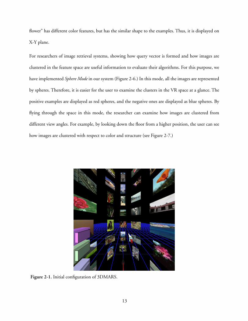
When the system starts, it displays images aligned in front of the user like a gallery (Figure 2-1.) As the
user moves, the images rotate to face the user. These images are randomly chosen by the system. When
the user touches one of the images by the wand, the image is highlighted and the filename is displayed
below it. By moving the wand (or mouse) the image can be moved to any position. The user can select
an image as relevant (i.e., a query example) by pressing a wand/mouse button. More than one image
11
can be selected. The selected images are displayed with red frames. In order to deselect an image, the
user presses the button again. S/he can also specify an image as a negative example. The negative
examples are displayed with blue frames. Moreover, the users can fly-through in the space with joystick.
To prevent the user from getting lost in the space, a virtual compass is provided on the floor. Three
arrows of the compass are always facing X-axis, Y-axis, and Z-axis respectively (Figure 2-5.)
When the user presses the QUERY button on the left wall, the system retrieves and displays the most
similar images from the image database (Figure 2-4.) The locations of the images are determined by
the similarity the query images. The X-axis, Y-axis and Z-axis represent color, texture and structure of
the images respectively. The more similar an image is, the closer to the origin of the space it is located.
If the user finds another relevant (or irreverent) image in the result set, s/he selects it with the wand as
an additional relevant (or irrelevant) example and presses the QUERY button again. By repeatedly
picking up new images, the query is improved incrementally and additional relevant images of the
user’s interest are clustered near the origin (Figure 2-5.)
Figure 2-4 shows the result after a user selects one “red flower” image as a positive example. Because
only one example is specified, the system assumes every feature is equally important. As a result, various
types of images are displayed. From this result, the user can give another feedback by selecting more
“red flower” images. In this example, the total number of images is 50.
Figure 2-5 shows the resulting visualization after the user selected two “red flower” images as query
examples. More pictures of flower are clustered around the origin. Here, the green arrow means the
“Color (X)” axis, the blue arrow means the “Texture (Y)” axis, and the red arrow means “Edge structure
(Z)” axis. The “Red flower” pictures have very similar color features to the query examples but have
different texture and structure. Therefore, they are displayed on Y-Z plane. Meanwhile, The “white
12
flower” has different color features, but has the similar shape to the examples. Thus, it is displayed on
X-Y plane.
For researchers of image retrieval systems, showing how query vector is formed and how images are
clustered in the feature space are useful information to evaluate their algorithms. For this purpose, we
have implemented Sphere Mode in our system (Figure 2-6.) In this mode, all the images are represented
by spheres. Therefore, it is easier for the user to examine the clusters in the VR space at a glance. The
positive examples are displayed as red spheres, and the negative ones are displayed as blue spheres. By
flying through the space in this mode, the researcher can examine how images are clustered from
different view angles. For example, by looking down the floor from a higher position, the user can see
how images are clustered with respect to color and structure (see Figure 2-7.)
Figure 2-1. Initial configuration of 3DMARS.
13

Figure 2-2. 3D MARS in CAVE
Figure 2-3. 3D MARS on a desktop VR
14

Figure 2-4. The result after the user selected one “red flower” picture (in Fixed axes mode.) Thequery example is displayed near the origin.
Figure 2-5. The result after the user selected another “flower” images. Red flowers of differenttexture are aligned along the red arrow.
15

Figure 2-6. The Sphere Mode. The number of images is 100.
Figure 2-7. The sphere mode from a different view angle (from the zenith of the space.)Relationship between color and structure is visualized
16
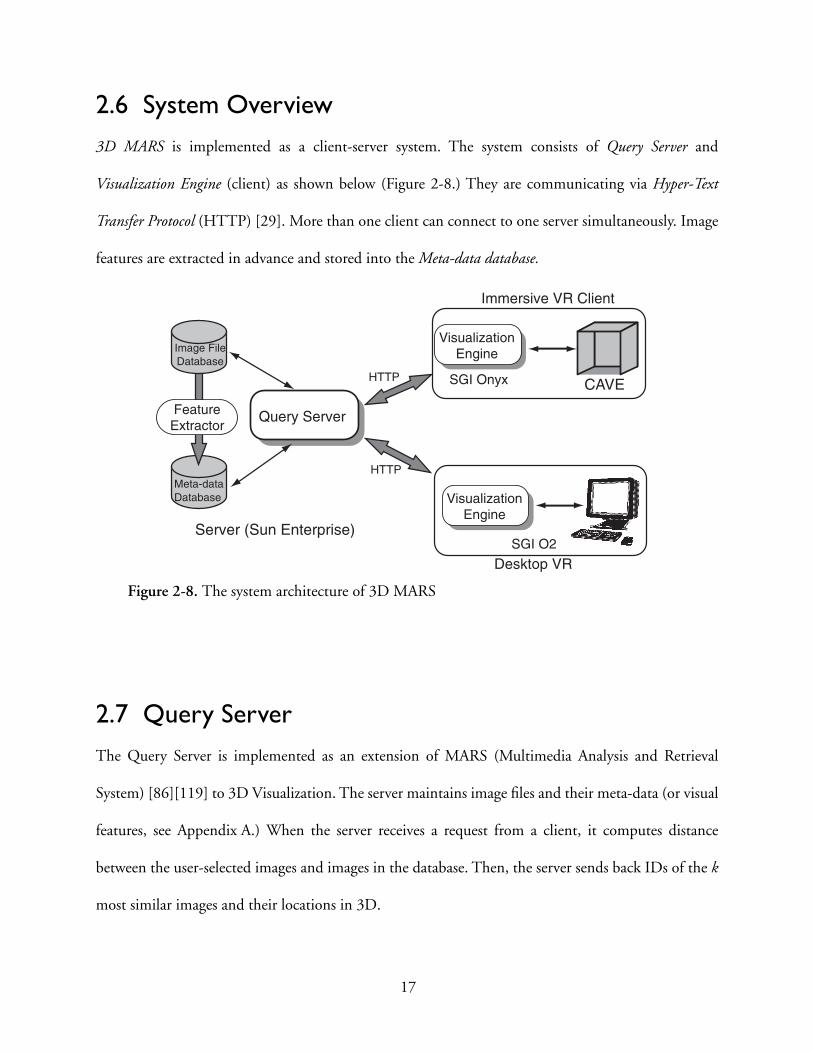
2.6 System Overview3D MARS is implemented as a client-server system. The system consists of Query Server and
Visualization Engine (client) as shown below (Figure 2-8.) They are communicating via Hyper-Text
Transfer Protocol (HTTP) [29]. More than one client can connect to one server simultaneously. Image
features are extracted in advance and stored into the Meta-data database.
2.7 Query ServerThe Query Server is implemented as an extension of MARS (Multimedia Analysis and Retrieval
System) [86][119] to 3D Visualization. The server maintains image files and their meta-data (or visual
features, see Appendix A.) When the server receives a request from a client, it computes distance
between the user-selected images and images in the database. Then, the server sends back IDs of the k
most similar images and their locations in 3D.
Query Server
CAVEHTTP
HTTP
SGI Onyx
Server (Sun Enterprise)
Immersive VR Client
Meta-dataDatabase Visualization
Engine
VisualizationEngine
SGI O2
Desktop VR
Image FileDatabase
FeatureExtractor
Figure 2-8. The system architecture of 3D MARS
17

2.7.1 Total Ranking vs. Feature Ranking
In the original MARS system [86], the ranking of the similar images are based on the weighted
combination of the all three features. The weight of each feature is computed from query examples. In
early stage of user interaction loop, however, the user may specify only one example. In this case, the
query server cannot tell which feature is important. Therefore, the system assumes every feature is
equally important. As a result, an image is considered to be relevant only when every feature is close to
the query. This can cause the search to fall into a local minimum.
To remedy this problem, we use two ranking strategy: Feature Ranking and Total Ranking. The Feature
Ranking is a ranking with respect to only one group of the features. First, for each feature group
, the system computes a query vector based on the positive
examples specified by the user. Next, it computes feature distance of each image n in the database
as follows,
(2-1)
where is the k th component of the i-th feature, is the k-th component of . The weight
is the inverse of the standard deviation of ( ),
(2-2)
Then, the feature ranking is computed by comparing ( ). In addition, the value
is also used to determine the location along the corresponding axis in fixed axes mode described later.
After the Feature Ranking is computed, the system combines each feature distance into the total
distance . The total distance of image n is the weighted sum of each ,
(2-3)
i Color, Texture, Structure{ }= qi
dni
dni wik xnik qik–( )k∑=
xnik qik qi wik
xnik n 1…N=
wik1σik-------=
dni n 1 2…N,= dni
dni
Dn dni
Dn uT dn=
18
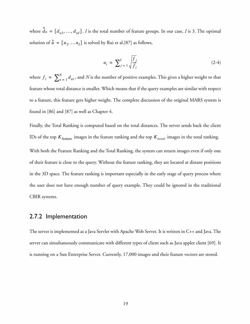
where . I is the total number of feature groups. In our case, I is 3. The optimal
solution of is solved by Rui et al.[87] as follows,
(2-4)
where , and N is the number of positive examples. This gives a higher weight to that
feature whose total distance is smaller. Which means that if the query examples are similar with respect
to a feature, this feature gets higher weight. The complete discussion of the original MARS system is
found in [86] and [87] as well as Chapter 4.
Finally, the Total Ranking is computed based on the total distances. The server sends back the client
IDs of the top images in the feature ranking and the top images in the total ranking.
With both the Feature Ranking and the Total Ranking, the system can return images even if only one
of their feature is close to the query. Without the feature ranking, they are located at distant positions
in the 3D space. The feature ranking is important especially in the early stage of query process where
the user does not have enough number of query example. They could be ignored in the traditional
CBIR systems.
2.7.2 Implementation
The server is implemented as a Java Servlet with Apache Web Server. It is written in C++ and Java. The
server can simultaneously communicate with different types of client such as Java applet client [69]. It
is running on a Sun Enterprise Server. Currently, 17,000 images and their feature vectors are stored.
dn dn1 … dnI, ,[ ]=
u u1 …uI,[ ]=
ui
f j
f i-----
j 1=
I∑=
f i dnin 1=N∑=
K feature Ktotal
19
2.8 Visualization EngineThe Visualization Engine takes a request from the user, sends the request to the server and receives the
result from the server. Then it visualizes the resulting images in VR space. In the immersive display, the
images are displayed on the four walls of CAVE, which is a projection-based Virtual Reality system.
When the user pushes the QUERY button, it sends the IDs of the selected (positive or negative) images
to the server. The requests are sent as a “GET” command of HTTP. When the reply is returned, the
client receives a list of IDs of the k most similar images and their locations. Next, it downloads all the
corresponding image files (such as JPEG files) from the image database. Finally, these images are
displayed on the virtual space. The system can display an arbitrary number of images on the VR space
as long as resources (texture memory) are available. In our environment, 50 to 200 images are
displayed. In the Sphere mode, more data can be displayed simultaneously because the image textures
do not have to be stored in the memory.
This component is written in C++ with OpenGL and CAVE library. The immersive version of the
visualization engine is running on a twelve-processor Silicon Graphics Onyx 2. Each wall of the CAVE
is drawn by a dedicated processor. Loaded image data are stored on a share memory and accessed from
these processors. For the desktop VR version, the system is running on SGI O2.
2.8.1 Projection Strategies
In order to project the high dimensional feature space into 3D space, we take two different approaches:
Static Axes and Dynamic Axes.
20

2.8.1.1 Static Axes
In the static axes approach, the meanings of X, Y, and Z-axis are fixed to some extent. In our
implementation, the X, Y and Z always mean the distance with respect to Color, Texture and Structure,
respectively. The location of each image is determined by the weighted sum of the corresponding
feature distance computed in the Query Server as described in Eq. 2-1. Therefore, for each axis, the
system automatically chooses an appropriate combination of features from the corresponding feature
group.
Because the meanings of the axes do not change for each interaction, the user can use the axes to obtain
a context of image searching. This makes navigation in the VR space easier. The problem of static axes
approach is that some axes (a group of features) may not give any useful information to the user. For
example, if none of the texture features are significant, the Y-axis does not have any meaning.
2.8.1.2 Dynamic Axes
In the dynamic axes, the meanings of the axes change for every interaction. The location of images is
determined by projecting the full 34 dimensional feature vector into a three dimensional space. Many
techniques have been proposed for this purpose. Because our goal is to provide a fully interactive
visualization, computationally expensive method such as MDS [52] is not suitable. In stead, we use
faster FastMap [27] method developed by Faloutsos et al. FastMap takes a distance matrix of points and
recursively maps points into lower dimensional hyperplanes. FastMap requires only
computation, where N is the number of images and k is the desired dimension.
First, we feed the raw feature vectors of the retrieved images (including the query vector) into FastMap.
Here, there is no distinction among color, texture and structure feature groups. They are combined into
one 34 dimensional vectors. After FastMap projects the image features onto 3D, we translate the entire
O Nk( )
21

VR space so that the location of the query vector matches the origin of the space. This guarantees that
the distance between an image and the origin always represents the degree of similarity to the query
example. The advantage of this approach is that the system requires only the feature vectors of the
images to discriminate the images. The disadvantage is that because the meanings of the directions are
always changing, the user may be confused.
2.9 ConclusionIn this chapter, we proposed a new interactive visualization system for Content-Based Image Retrieval,
named 3D MARS. Compared with the traditional CBIR systems, more images can be displayed
simultaneously in 3D space. By giving different meaning to each axis, the user can browse the retrieved
images with respect to three different criteria at a glance. In addition, using the feature ranking, the
system can display images that could be ignored in the traditional CBIR systems. Furthermore, unlike
other 3D image visualization systems, where mapping to 3D space is fixed, 3D MARS can interactively
optimize the visualization strategies in response to the users’ feedback.
With the Sphere display mode, the 3D MARS provides CBIR researcher with a powerful analyzing
tool. By flying through the space, the user can analyze image clusters from different viewpoints.
2.10 Possible ImprovementIn this section, we discuss possible improvements in the user interaction and the display strategies of
the system.
22

2.10.1 Integration of Browsing and Searching
One limitation of our system is that the user has to find an initial query example from a random
selection. The user has to repeat the random query until any interesting image is found. Chen et al.
[20] proposed a technique to automatically generate a tree structure of image database. By following
this hierarchy, the user can effectively browse images.
Pecenovic et al. [120] integrated image browsing and query-by-example. In their system, images are
organized into hierarchical structure by recursively clustering images by k-means algorithm. At every
level, each node is represented by image that is the closest to the centroid of the cluster. The user can
switch from the browsing to query-by-example anytime.
If some images in the database have text annotation, these information can be used as a starting point
of a query. We plan to integrate several browsing strategies into 3D MARS.
2.10.2 Migrating to 6-Sided CAVE
The current system was developed on 4-sided CAVE, which has projectors on the front, right, left, and
floor. Because the system does not have projectors above and behind the users, our display algorithm
was limited. The query results have to be displayed only on the front side of the user. We are going to
implement the system on 6-sided CAVE (CUBE). Because 6-sided CAVE provides the user with a full
field of view, there are no limitations on the visualization strategies. On the 6-sided CAVE, we are going
to investigate more effective and intuitive user interface. For example, we can rank retrieved images in
six different ways.
23
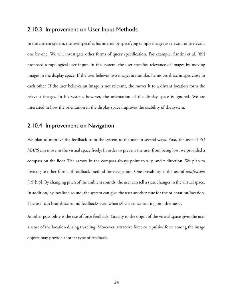
2.10.3 Improvement on User Input Methods
In the current system, the user specifies his interest by specifying sample images as relevant or irrelevant
one by one. We will investigate other forms of query specification. For example, Santini et al. [89]
proposed a topological user input. In this system, the user specifies relevance of images by moving
images in the display space. If the user believes two images are similar, he moves these images close to
each other. If the user believes an image is not relevant, the moves it to a distant location form the
relevant images. In his system, however, the orientation of the display space is ignored. We are
interested in how the orientation in the display space improves the usability of the system.
2.10.4 Improvement on Navigation
We plan to improve the feedback from the system to the user in several ways. First, the user of 3D
MARS can move in the virtual space freely. In order to prevent the user from being lost, we provided a
compass on the floor. The arrows in the compass always point to x, y, and z direction. We plan to
investigate other forms of feedback method for navigation. One possibility is the use of sonification
[15][95]. By changing pitch of the ambient sounds, the user can tell a state changes in the virtual space.
In addition, by localized sound, the system can give the user another clue for the orientation/location.
The user can hear these sound feedbacks even when s/he is concentrating on other tasks.
Another possibility is the use of force feedback. Gravity to the origin of the virtual space gives the user
a sense of the location during traveling. Moreover, attractive force or repulsive force among the image
objects may provide another type of feedback.
24

2.10.5 Multi-Cluster Display
In the prototype, the system computes one query vector from the positive and negative examples.
Therefore, the user has to select only one set of similar examples. Querying two different types of
images simultaneously is not allowed. Therefore, the system shows only one cluster for each query. For
some users, however, querying more than one type of images might be desired. The important question
is how to display the relationship between two different image classes in the display space. To this end,
modification of the classification algorithm may be required.
25
Chapter 3
Group-Oriented User Interface for Digital Image Retrieval and Management
3.1 User Interface Support for Content-based Image RetrievalIn Content-based Image Retrieval (CBIR), experimental (i.e., Trial-and-Error) query is essential for
successful retrieval. Unfortunately, the traditional user interfaces are not suitable for trying different
combinations of query examples. This is because first, these systems assume query examples are added
incrementally. Second, the query specification and result display are done on the same workspace.
Once the user removes an image from the query examples, the image may disappear from the user
interface. In addition, it is difficult to combine the result of different queries.
In this chapter, we propose a new user interface for the Content-based Image Retrieval named
ImageGrouper. ImageGrouper is a Group-Oriented User Interface in that each operation is done by
creating groups of images. The users can interactively compare different combinations of query
examples by dragging and grouping images on the workspace (Query-by-Group.) Because the query
26
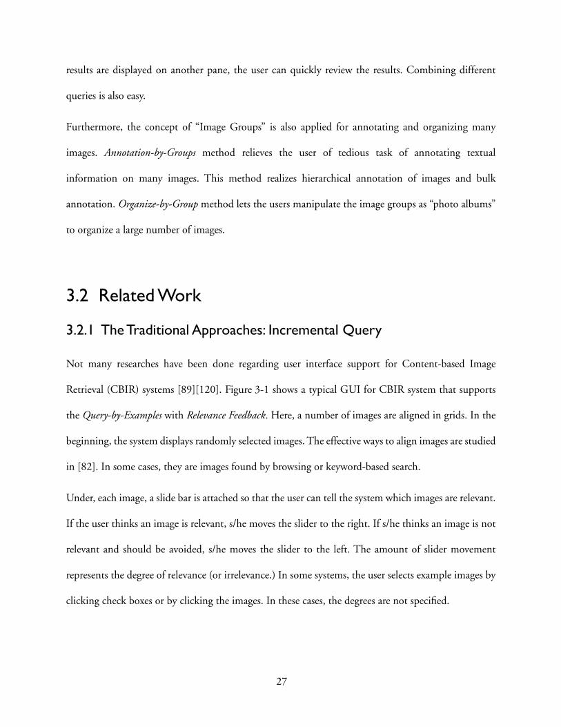
results are displayed on another pane, the user can quickly review the results. Combining different
queries is also easy.
Furthermore, the concept of “Image Groups” is also applied for annotating and organizing many
images. Annotation-by-Groups method relieves the user of tedious task of annotating textual
information on many images. This method realizes hierarchical annotation of images and bulk
annotation. Organize-by-Group method lets the users manipulate the image groups as “photo albums”
to organize a large number of images.
3.2 Related Work
3.2.1 The Traditional Approaches: Incremental Query
Not many researches have been done regarding user interface support for Content-based Image
Retrieval (CBIR) systems [89][120]. Figure 3-1 shows a typical GUI for CBIR system that supports
the Query-by-Examples with Relevance Feedback. Here, a number of images are aligned in grids. In the
beginning, the system displays randomly selected images. The effective ways to align images are studied
in [82]. In some cases, they are images found by browsing or keyword-based search.
Under, each image, a slide bar is attached so that the user can tell the system which images are relevant.
If the user thinks an image is relevant, s/he moves the slider to the right. If s/he thinks an image is not
relevant and should be avoided, s/he moves the slider to the left. The amount of slider movement
represents the degree of relevance (or irrelevance.) In some systems, the user selects example images by
clicking check boxes or by clicking the images. In these cases, the degrees are not specified.
27

When the “Query” button is pressed, the system computes the similarity between selected images and
the database images, then retrieves the N most similar images. The grid images are replaced with the
retrieved images. These images are ordered based on the degree of similarity.
If the user finds additional relevant images in the result set, s/he selects them as new query examples.
If a highly irrelevant image appears in the result set, the user can select it as a negative example. Then,
the user press the “Query” button again. The user can repeat this process until s/he is satisfied. In some
systems, the users are allowed to directly weight the importance of image features such as color and
texture.
In [96], Smeulders et al. classified Query by Image Example and Query by Group Example into two
different categories. From user interface viewpoint, however, these two are very similar. The only
difference is whether the user is allowed to select multiple images or not. In this chapter, we classify
Figure 3-2. Example of “More is not necessarily better”. The left is the case of one example,the right is the case of two examples.
Query
Results
Query Results
28
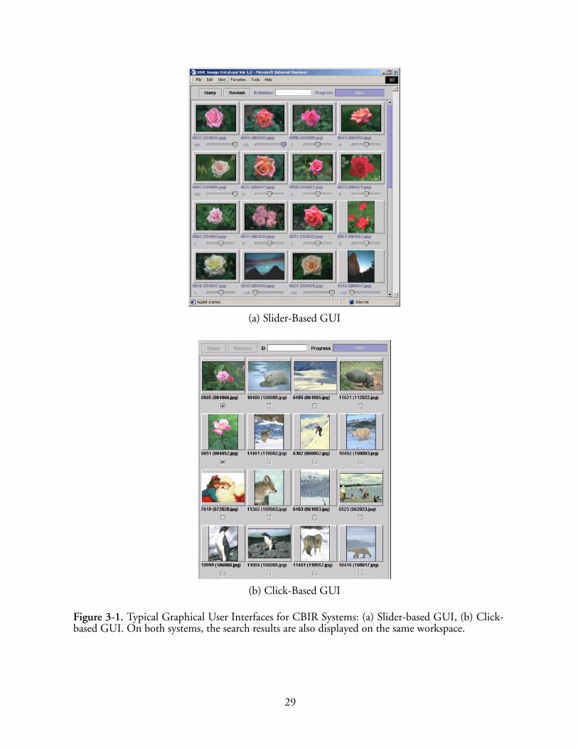
Figure 3-1. Typical Graphical User Interfaces for CBIR Systems: (a) Slider-based GUI, (b) Click-based GUI. On both systems, the search results are also displayed on the same workspace.
(a) Slider-Based GUI
(b) Click-Based GUI
29

both approaches as Query by Examples method. In stead, we use term “Query by Groups” to refer our
new model of query specification method described later.
3.2.2 Limitation of Incremental Query
The traditional Query-by-Example approach has several drawbacks. First of all, these systems assume
that “the More Query Examples are Available, the Better Result We Can Get.” Therefore, the users are
supposed to search images incrementally by adding new example images from the result of the previous
query. However, this assumption is not always true. Additional query examples may contain undesired
features and degenerate the retrieval performance.
Figure 3-2 shows an example of situations when more query examples could lead to worse results. In
this example, the user is trying to retrieve pictures of cars. The left column shows the query result when
only one image of “car” is used as a query example. The right column shows the result of two query
examples. The results are ordered based on the similarity ranks. In both cases, the same relevance
feedback algorithm (Section 3.9.1.2 and [86]) was used and tested on Corel image set of 17,000
images. In this example, even if this additional example image looks visually good for human eyes, it
introduces undesirable features into the query. Thus, no car image appears in the top 8 images. An
image of car appears in the rank 13th for the first time.
This example is not a special case. It happens often in image retrieval and confuses the users. This
problem happens because of Semantic Gap [89][96] between the high-level concept in the user’s mind
and the extracted features of images. Furthermore, finding good combinations of query examples is
very difficult because image features are numerical values that are impossible to be estimated by human.
The Only way to find the right combination is trial and error. Otherwise, the user can be trapped in a
small part of image database [120].
30
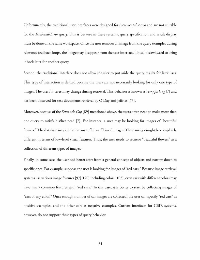
Unfortunately, the traditional user interfaces were designed for incremental search and are not suitable
for the Trial-and-Error query. This is because in these systems, query specification and result display
must be done on the same workspace. Once the user removes an image from the query examples during
relevance feedback loops, the image may disappear from the user interface. Thus, it is awkward to bring
it back later for another query.
Second, the traditional interface does not allow the user to put aside the query results for later uses.
This type of interaction is desired because the users are not necessarily looking for only one type of
images. The users’ interest may change during retrieval. This behavior is known as berry picking [7] and
has been observed for text documents retrieval by O’Day and Jeffries [73].
Moreover, because of the Semantic Gap [89] mentioned above, the users often need to make more than
one query to satisfy his/her need [7]. For instance, a user may be looking for images of “beautiful
flowers.” The database may contain many different “flower” images. These images might be completely
different in terms of low-level visual features. Thus, the user needs to retrieve “beautiful flowers” as a
collection of different types of images.
Finally, in some case, the user had better start from a general concept of objects and narrow down to
specific ones. For example, suppose the user is looking for images of “red cars.” Because image retrieval
systems use various image features [97][120] including colors [105], even cars with different colors may
have many common features with “red cars.” In this case, it is better to start by collecting images of
“cars of any color.” Once enough number of car images are collected, the user can specify “red cars” as
positive examples, and the other cars as negative examples. Current interfaces for CBIR systems,
however, do not support these types of query behavior.
31

3.2.3 El Ninõ System
Another interesting approach for the Query-by-Examples has been proposed by Santini et.al [89]. In
their El Ninõ system, the user specifies a query by mutual distance between example images. The user
drags images on the workspace so that the more similar images (in the user’s mind) are located closer
to each other. The system then reorganizes the images’ locations reflecting the user’s intent. There are
two drawbacks in El Ninõ system. First, it is unknown to the users how close similar images should be
located and how far negative examples should be apart from good examples. It may take a while for the
user to learn “the metric system” used in this interface.
The second problem is that like traditional interfaces, query specification and result display are done
on the same workspace. Thus, the user’s previous decision (in the form of the mutual distance between
the images) is overridden by the system when it displays the results. This makes trial-and-error query
difficult. Given the analogue nature of this interface, trial-and-error support might be essential. Even
if the user gets an unsatisfactory result, there is no way to redo the query with a slightly different
configuration. Any experimental result is not provided in the chapter.
3.3 Query-by-Groups with ImageGrouperWe developed a new user interface for CBIR systems named ImageGrouper. The design goal of
ImageGrouper is to improve the flexibility and usability of image retrieval. In this system, a new concept
for the relevance feedback, called Query-by-Groups was introduced. The Query-by-Groups mode is an
extension of the Query-by-Example mode described above. The major difference is that while the
Query-by-Example handles the images individually, in the Query-by-Group, a “group of images” is
considered as the basic unit of the query.
32
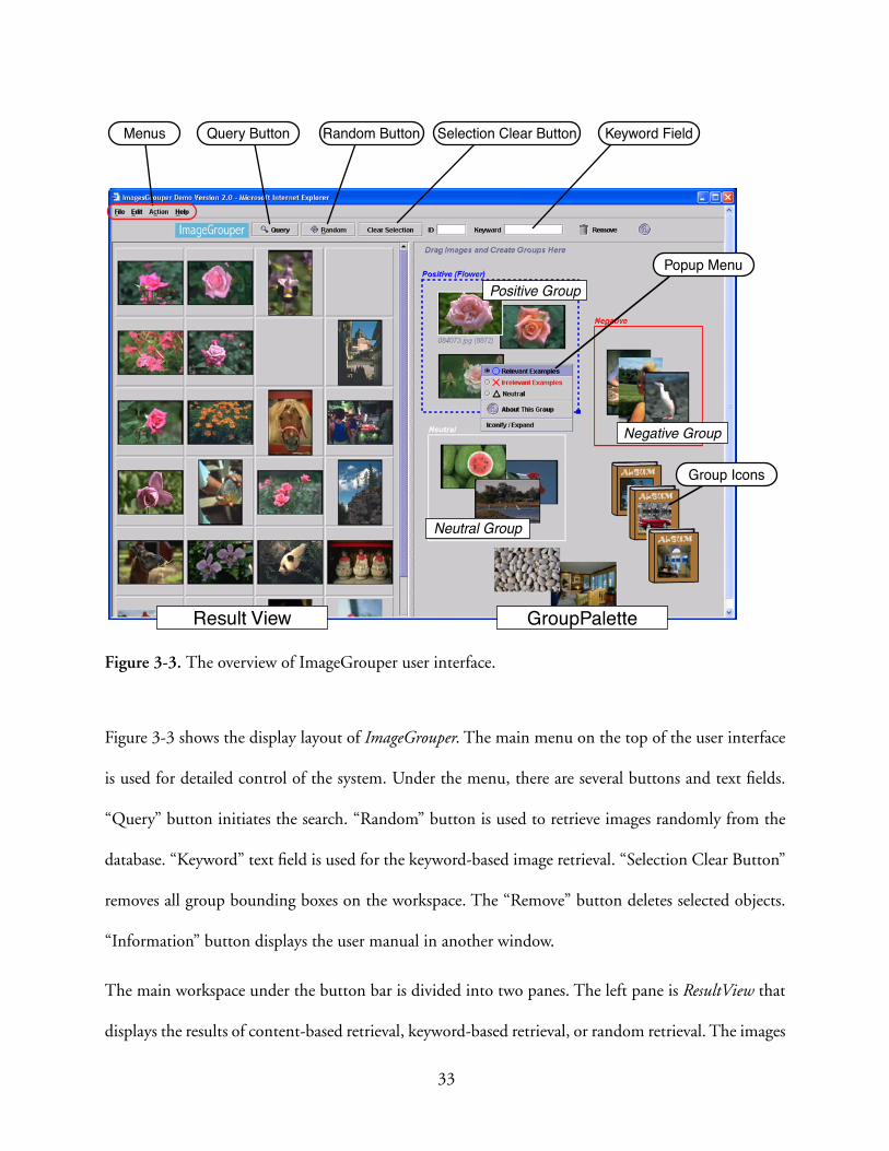
Figure 3-3 shows the display layout of ImageGrouper. The main menu on the top of the user interface
is used for detailed control of the system. Under the menu, there are several buttons and text fields.
“Query” button initiates the search. “Random” button is used to retrieve images randomly from the
database. “Keyword” text field is used for the keyword-based image retrieval. “Selection Clear Button”
removes all group bounding boxes on the workspace. The “Remove” button deletes selected objects.
“Information” button displays the user manual in another window.
The main workspace under the button bar is divided into two panes. The left pane is ResultView that
displays the results of content-based retrieval, keyword-based retrieval, or random retrieval. The images
Figure 3-3. The overview of ImageGrouper user interface.
Result View
Positive Group
Negative Group
Popup Menu
Group Icons
Neutral Group
Query Button Keyword FieldRandom Button Selection Clear ButtonMenus
GroupPalette
33
are tiled in a grid. This is very similar to the traditional user interfaces (Figure 3-1) except for there are
no sliders or buttons under the images. The right pane is GroupPalette, where the user creates and
manages image groups by drawing bounding boxes as described in the following sections. Unlike the
ResultView, the user can move the images to arbitrary positions within the palette.
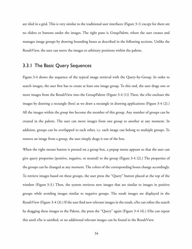
3.3.1 The Basic Query Sequences
Figure 3-4 shows the sequence of the typical image retrieval with the Query-by-Group. In order to
search images, the user first has to create at least one image group. To this end, the user drags one or
more images from the ResultView into the GroupPalette (Figure 3-4 (1)) Then, the s/he encloses the
images by drawing a rectangle (box) as we draw a rectangle in drawing applications (Figure 3-4 (2).)
All the images within the group box become the member of this group. Any number of groups can be
created in the palette. The user can move images from one group to another at any moment. In
addition, groups can be overlapped to each other, i.e. each image can belong to multiple groups. To
remove an image from a group, the user simply drags it out of the box.
When the right mouse button is pressed on a group box, a popup menu appears so that the user can
give query properties (positive, negative, or neutral) to the group (Figure 3-4 (2).) The properties of
the groups can be changed at any moment. The colors of the corresponding boxes change accordingly.
To retrieve images based on these groups, the user press the “Query” button placed at the top of the
window (Figure 3-3.) Then, the system retrieves new images that are similar to images in positive
groups while avoiding images similar to negative groups. The result images are displayed in the
ResultView (Figure 3-4 (3).) If the user find new relevant images in the result, s/he can refine the search
by dragging these images to the Palette, the press the “Query” again (Figure 3-4 (4).) S/he can repeat
this until s/he is satisfied, or no additional relevant images can be found in the ResultView.
34

When a group is specified as Neutral (displayed as a white box), this group does not contribute to the
search at the moment. This group can be turned to a positive or negative group later for another
retrieval. If a group is Positive (displayed as a blue box), the system uses common features among the
images in the group. On the other hand, if a group is given Negative (red box) property, the common
features in the group are used as negative feedbacks. The user can specify multiple groups as positive
or negative. In this case, these groups are merged into one group, i.e., the union of the groups is taken.
The detail of the algorithm is described in Section 3.9.1.2.
While the user created only one group in Figure 3-4, the user can create multiple groups on the
workspace. Figure 3-3 is an example of three groups. As in Figure 3-4, the user is retrieving images of
“flowers.” In the GroupPalette, three flower images are grouped as a positive group. On the right of this
group, a red box is representing a negative group that consists of only one image. Below the “flowers”
group, there is a neutral group (white box), which is not used for retrieval at this moment. Images can
be moved out of any groups in order to temporarily remove images from the groups.
The gestural operations of ImageGrouper are similar to file operations of a Window-based Operating
Systems. Furthermore, because the user’s mission is to collect images, the operation “Dragging Images
into a Box” naturally matches the user’s cognitive state.
35
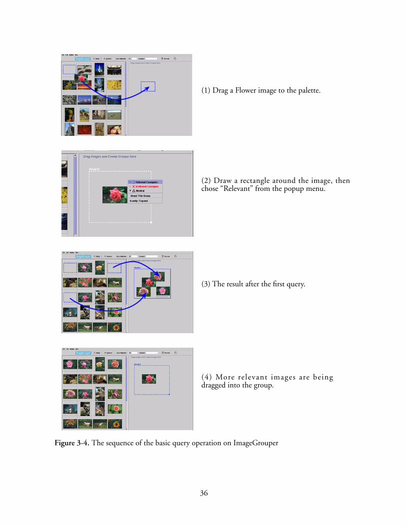
(1) Drag a Flower image to the palette.
(2) Draw a rectangle around the image, thenchose “Relevant” from the popup menu.
(3) The result after the first query.
(4) More relevant images are beingdragged into the group.
Figure 3-4. The sequence of the basic query operation on ImageGrouper
36

3.4 The Flexibility of Query-by-GroupsImageGrouper provides greater flexibility to image retrieval with the Query-by-Groups. In this section,
we describe how the Query-by-Groups method improve the relevance feedback for content-based
image retrieval.
3.4.1 Trial and Error Query by Mouse Dragging
In ImageGrouper, the images can be easily moved between the groups by mouse drags. In addition, the
neutral groups and space outside any groups in the palette can be used as storage area [49] for the images
that are not used at the moment. They can be reused later for another query. It makes trial and error
of relevance feedbacks easy. The user can quickly explore different combinations of query examples by
dragging the images into or out of the boxes. Moreover, the query specification that the user made is
preserved and visible in the palette. Thus, it is easy to modify the previous decision when the query
result is not satisfactory. In Section 3.5, we will evaluate the effects of the experimental query on the
image retrieval performances.
3.4.2 Groups in a Group
ImageGrouper allows the users to create a new group within a group (Groups in a Group.) With this
method, the user begins with collecting relatively generic images first, then narrows down to more
specific images.
Figure 3-6 shows an example of Groups in a Group. Here, the user is looking for “Red cars.” When s/
he does not have enough number of examples, however, the best way to start is to retrieve images of
“cars with any color.” This is because these images may have many common features with red car
37
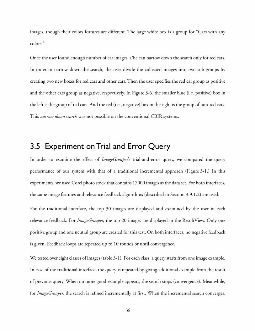
images, though their colors features are different. The large white box is a group for “Cars with any
colors.”
Once the user found enough number of car images, s/he can narrow down the search only for red cars.
In order to narrow down the search, the user divide the collected images into two sub-groups by
creating two new boxes for red cars and other cars. Then the user specifies the red car group as positive
and the other cars group as negative, respectively. In Figure 3-6, the smaller blue (i.e. positive) box in
the left is the group of red cars. And the red (i.e., negative) box in the right is the group of non-red cars.
This narrow down search was not possible on the conventional CBIR systems.
3.5 Experiment on Trial and Error QueryIn order to examine the effect of ImageGrouper’s trial-and-error query, we compared the query
performance of our system with that of a traditional incremental approach (Figure 3-1.) In this
experiments, we used Corel photo stock that contains 17000 images as the data set. For both interfaces,
the same image features and relevance feedback algorithms (described in Section 3.9.1.2) are used.
For the traditional interface, the top 30 images are displayed and examined by the user in each
relevance feedback. For ImageGrouper, the top 20 images are displayed in the ResultView. Only one
positive group and one neutral group are created for this test. On both interfaces, no negative feedback
is given. Feedback loops are repeated up to 10 rounds or until convergence.
We tested over eight classes of images (table 3-1). For each class, a query starts from one image example.
In case of the traditional interface, the query is repeated by giving additional example from the result
of previous query. When no more good example appears, the search stops (convergence). Meanwhile,
for ImageGrouper, the search is refined incrementally at first. When the incremental search converges,
38

trial and error search is applied by moving some images out of the positive group into a neutral group
(This means that the number of positive examples is temporarily decreased.) Then, the search is refined
incrementally again until another convergence occurs. The user repeats this until trial and error query
has no effect.
Figure 3-5 shows the number of correctly retrieved images after the convergence (or the 10th rounds.)
This value is proportional to the recall rate. Thus, larger value means better retrieval performance.
Table 3-1 shows the number of relevance feedback loops until convergence. The value 10 means the
query did not converge before the 10th round.
Clearly, ImageGrouper can achieve better retrieval (i.e., higher recall) even if underlying technologies
(relevance feedback algorithm and visual features) are identical. In addition, the search with
ImageGrouper is less likely to converge prematurely even when the search with the traditional interface
converges into small number of images after a few iterations. This result suggests the importance of
support for the trial-and-error query.
Meanwhile, Query-by-Group can introduce a new problem. In an experimental query, the users need
to decide which images should be included in the query set. Often, the user expects the search to
improve by adding or removing an image. This task is not always easy to predict. Although
ImageGrouper enables fast trial-and-error, the user may have to try many different combinations until
the search improves. Unfortunately, it is difficult to automate this process because the judgement of
the query results is subjective and depends on the user. However, it is still desirable that the system
suggests some promising query combinations. For example, the system can find an outlier in the
current set of query examples.
39
Table 3-1. The number of feedback loops until convergence.10 means that it did not converge until 10th round
Object Traditional Grouper
Red Car 4 10
Tiger 3 10
Bird 4 8
Yellow Flower 3 10
Citrus 2 4
Polar Bear 5 10
Elephant 3 10
Swimmer 2 10
0
5
10
15
20
25
30
Hits
TraditionalImageGrouper
Image Class
Red Car
Tiger Bird YellowFlower
Citrus PolarBear
Elephant Swimmerr
Figure 3-5. The number of hits until the 10th round or convergence
40

3.6 Text Annotations on ImagesKeyword-based search is a very powerful method for searching images. The problem is that it works
well only when all the images are annotated with textual information. For commercial photo stocks, it
may be feasible to add keywords to all images manually. For home users, however, it is too tedious.
When keyword search is integrated with CBIR like our system and [120], keyword-based search can
be used to find the initial query examples for content-based search. For this scheme, the user does not
have to annotate all images. It is very important to provide easy and quick ways to annotate text on
many images.
3.6.1 Current Approaches for Text Annotation
The most primitive way for annotation is to select an image, then type in keywords. Because this
interaction requires the user to switch between mouse and keyboard repeatedly, it is too frustrating for
a large image database.
Several researchers have proposed smarter user interfaces for keyword annotation on images. In Bulk
Annotation method of FotoFile [53], the user selects multiple images on the display, selects several
attribute/value pairs from a menu, and then presses the “Annotate” button. Therefore, the user can add
the same set of keywords on many images at the same time. To retrieve images, the user selects entries
from the menu, and then presses the “Search” button. Because of visual and gestural symmetry [53], the
user needs to learn only one tool for both annotation and retrieval.
PhotoFinder [94] introduced drag-and-drop method, where the user selects a label from a scrolling list,
then drags it directly onto an image. Because the labels remain visible at the designated location on the
images and these locations are stored in the database, these labels can be used as “captions” as well as
41
for keyword-based search. For example, the user can annotate the name of a person directly on his/her
portrait in the image, so that other users can associate the person with his/her name. When the user
needs new words to annotate, s/he adds them to the scrolling list. Because the user drags keywords into
individual images, bulk annotation is not supported in this system.
3.6.2 Annotation by Groups
Most home users do not want to annotate images one by one, especially when the number of images
is large. In many cases, the same set of keywords is enough for several images. For example, a user may
just want to annotate “My Roman Holiday, 1997” on all images taken in Rome. Annotating the same
keywords repeatedly is painful enough to discourage him/her from using the system.
ImageGrouper introduces Annotation-by-Groups method where keywords are annotated not on
individual image, but on groups. As in Query-by-Groups, the user first creates a group of images by
dragging images from the ResultView into the GroupPalette and drawing a rectangle around them. In
order to give keywords to the group, the user opens Group Information Window by selecting “About
This Group” from the pop-up menu (Figure 3-3.) In this window, arbitrary number of words can be
added. Because the users can simultaneously annotate the same keywords on a number of images,
annotation becomes much faster and less error prone. Although Annotation-by-Groups is similar to the
bulk annotation of FotoFile, there are several advantages described below.
3.6.2.1 Annotating New Images with the Same Keywords
In the bulk annotation [53], once the user finished annotating keywords to some images, there is no
fast way to give the same annotation to another image later. The user has to repeat the same steps (i.e.
select images, select keywords from the list, then press “Annotate”.) This is awkward when the user has
to add a large number of keywords. Meanwhile, in Annotation-by-Group, the system attaches
42

annotations not on each images, but on groups. Therefore, by dragging new images into an existing
group, the same keywords are automatically given to it. The user does not have to type the same words
again.
3.6.2.2 Hierarchical Annotation with Groups in a Group
In ImageGrouper, the user can annotate images hierarchically using Groups in a Group method
described above (Figure 3-6.) For example, the user may want to add new keyword “Trevi Fountain”
to only a part of the image group that has been labeled “My Roman Holiday, 97.” This is easily done
by creating a new sub-group within the group and annotating only on the sub-group.
In order to annotate hierarchically on FotoFile with bulk annotation, the user has to select a subset of
images that are already annotated, and then annotate them again with more keywords. On the other
hand, ImageGrouper allows the user to visually construct a hierarchy on the GroupPalette first, then
edit keywords on the Group Information Window. This method is more intuitive and less error prone.
3.6.2.3 Overlap between Images
An image often contains multiple objects or people. In such cases, the image can be referred in more
than one context. ImageGrouper support this multiple reference by allowing overlaps between image
groups, i.e., an image can belong to multiple groups at the same time. For example, in Figure 3-7, there
are two image groups: “Cloud” and “Mountains.” Because some images contain both cloud and
mountain, these images belong to both groups (in overlapped region.) Once these two groups are
annotated with “Cloud” and “Mountain” respectively, images in overlapped region are automatically
referred as “Cloud and Mountain.” This concept is not supported in other systems.
43
3.7 Organizing Images by GroupsIn the previous two sections, we described how ImageGrouper supports content-based query and
keyword annotation. These features are closely related and complementary to each other. In order to
annotate images, the user can collect visually similar images first, using content-based retrieval with
Query-by-Groups. Then s/he can annotate textual information to the group of collected images. After
this point, the user can quickly retrieve the same images using keyword-based search.
Conversely, the results of keyword-based search can be used as a starting point for content-based search.
This method is useful especially when the image database is only partially annotated or when the user
is searching images based on visual appearance only.
3.7.1 Photo Albums and Group Icons
As described above, ImageGrouper allows the groups to be overlapped. In addition, the user can attach
textual information on these groups. Therefore, the groups in ImageGrouper can be used to organize
pictures as “photo albums [53]” Similar concepts are proposed in FotoFile [53] and Ricoh’s Storytelling
system [6]. In both systems, albums are used for “slide shows” to tell stories to the other users.
In ImageGrouper, the user can convert a group into a Group Icon (Figure 3-3.) When the user selects
“Iconify” from the popup menu (Figure 3-3) images in the group disappear and a new icon for the
group appears in the GroupPalette. When the group has an overlap with another group, images in the
overlapped region remain in the display.
Furthermore, the users can manipulate those group icons as they handle individual images. They can
drag the group icons anywhere in the palette. The icons can be even moved into another group box
realizing Groups in a group.
44
Finally, group icons themselves can be used as examples for content-based query. A group icon can be
used as an independent query example or combined with other images and groups. In order to use a
group icon as a normal query group, the user right clicks the icon and opens a popup menu. Then, s/
he can select “relevant,” “irrelevant” or “neutral.” On the other hand, in order to combine a group icon
with other example images, the user simply draws a new rectangle and drags them into it.
Organize-by-Groups method described here is partially inspired by the Digital Library Integrated Task
Environment (DLITE) [24]. In DLITE, each text document and the search results is visually
represented by icons. The user can directly manipulate those documents in a workcenter (direct-
manipulation.) In [49], Jones proposed another graphical tool for query specification, named VQuery.
In VQuery, the user specifies the query by creating Venn diagrams. The number of matched documents
is displayed in the center of each circle.
While DLITE and VQuery are designed for text document retrieval systems [3], the idea of direct-
manipulation [24] is applicable more naturally to image databases. In text document database, it is
difficult to determine the contents of text documents from the icons. Therefore, the user has to open
another window to examine the detail [24] (in the case of DLITE, a web browser is opened.) On the
other hand, in image databases, images themselves (or their thumbnails) are the objects that the user
operates on. Therefore, instant judgment by the user is possible on a single workspace [120][96].
45

Red Cars Non-Red Cars
Figure 3-6. Groups in a group. In ImageGrouper, the user can create a hierarchy of image group. Inthis example, the entire group is “cars.” Once the whole group is annotated as “car,” the user onlyneed to type “red” to annotate the red cars.
Cars of any color
CAR
RED CAR OTHER CAR
“Red”
“Car”
Figure 3-7. Overlap between groups. Two images in the overlapped region contain both mountainand cloud. Once the two groups are annotated, the overlapped region are automatically annotatedwith both keywords.
Mountain
Cloud and Mountain
Cloud
46
3.8 Usability StudyEven if ImageGrouper provides a powerful search ability, the users cannot take advantages of the system
unless the system is easy to use. In order to compare the usability of ImageGrouper with the traditional
graphical user interfaces (GUIs), we conducted usability tests. ImageGrouper was compared with two
traditional GUIs: a simple Click-based Interface (Figure 3-1 (b)) and a Slider-based Interface (Figure 3-
1 (a).) An example of the Click-based Interface is QBIC [31] and an example of the Slider-based
Interface is the original MARS [86]. Each GUI employs different relevance feedback method and has
different expressiveness. For example, the Click-based GUI is very simple and easy to use, but only
positive feedback was allowed. The Slider-based GUI allows the user to specify the degree of relevance
(from -1.0 to 1.0.) Both the Click-based and the Slider-based lose the previous query information
when the search results are returned. Meanwhile, ImageGrouper requires drag-and-drop operations, but
it realizes a more flexible query with trial-and-error query. Therefore, it is very difficult to compare the
usabilities of these systems in the actual image retrieval scenarios. Instead, we compared the task
completion time and the error rate of the image selection tasks in a simplified scenario as described
below.
3.8.1 Experimental Settings
3.8.1.1 Subjects
Ten people volunteered to participate in this experiment. All subjects were familiar with the commonly
used widgets that require mouse operations such as sliders and check boxes. The ages ranged from 20’s
to 30’s. One was a female and nine were male. Most subjects did not have experiences in any content-
based image retrieval systems.
47

3.8.1.2 Apparatus
Both training and tests are conducted with a PC with Dual Intel Xeon 2GHz Processors with 1GB of
Main Memory running Windows XP. The PC was located in a small quiet room. The video card was
nVIDIA Quadro2 with 32MB Video RAM. For the display, a 17 inch LCD monitor set at 1280 by
960 in 32-bit color was used. All user operations were done with a Microsoft Optical USB Mouse.
Each system was implemented in Java2 (version 1.3.x) with Swing API. ImageGrouper requires slightly
more graphics computation than the other two because the images have to be dragged over the
workspace. Above specs, however, are more than enough to run each GUI smoothly, eliminating the
differences in the computational overhead. Note that ImageGrouper does not require such a high-spec
machines. It runs smoothly on average PCs or workstations.
3.8.2 Scenarios
3.8.2.1 Experimental Task
The task of this experiment is to find and select relevant images on each GUI. In each run, when a
subject presses the “start” button, a sample image and its description (in text) are displayed on a
separate window located to the left of the main GUI. At the same time, 16 different images are tiled
on the main GUI. Then, they are asked to find and select all images that are “semantically similar” to
the sample images. The correct images do not have to be visually similar to the sample image. For
example, if a sample image is a picture of a standing penguin and the description is “Penguin,” the
subject has to choose all pictures of penguins even if the pictures look different from the sample image
(for example a picture of two penguins lying on ice.)
Each user interface requires different operations to select the images. In the case of the Click-based
system, “Select” means simply clicking the pictures on the GUI. In the case of the Slider-based
48

Interface, the user selects an image by moving the slider to the right. For ImageGrouper, the images are
selected by dragging images from the ResultView to the GroupPalette. In any cases, the subjects can
examine all images without scrolling. When the subject believes every relevant image is selected, s/he
presses the “Next” button. Then the system displays the next problem (a new sample images and
another set of 16 images on the GUI.) For both trainings and experiments, the task was repeated 10
times with different sample images such as “elephant,” “flowers,” “airplane,” “cars,” and “fireworks.”
The number of the correct images was different from one problem to another. The size of each image
was fixed to 120 by 80 pixels (or 80 by 120.)
Each subject was tested with all three GUIs one by one. The order of the GUIs was randomly chosen
for each subject. For each interface, the subjects were first trained with the sample problems, then they
were tested with the same interface immediately after the training.
3.8.2.2 Training Session
Before the training and testing of each GUI began, each subject individually received a brief instruction
about the concept of the GUI (how to select and deselect images) and the procedure of the experiment.
Then, s/he was asked to conduct the image selecting operation on the GUI with 10 training problems
under the trainer’s supervision. Because the purpose of this training is to make him/her familiar with
the GUI, the subject was allowed to ask the trainer assistance during the session.
3.8.2.3 Experiment Session
After the subject became familiar enough with the user interface, the subject began the same procedure
with new problem sets. The number of images to be selected was not known to the subject and was
different for each problem. Unlike the training phase, the subject was encouraged to conduct the
operations as fast as possible and as accurate as possible. No question was allowed during the sessions.
49

The completion time and the number of errors (the number of images missed and the number of image
incorrectly selected) were recorded. The subjects were interviewed after the experiment.
3.8.3 The Results
3.8.3.1 Error Rate
To see the effects of the user interfaces on the accuracy of the tasks, we compared the number of missed
images and the number of incorrectly selected images during the image selection tasks. Table 3-2 shows
the total of 10 problems. The values are averaged over ten subjects. With each interface, the subjects
rarely selected wrong images (at most once in ten problems.) The differences among the user interfaces
was not significant (F(2, 27) = 0.144, p = .254).
Figure 3-8. The Usability Test Setting (Click-base GUI)
50
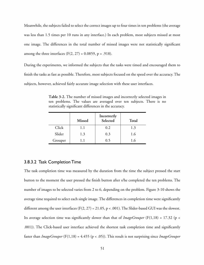
Meanwhile, the subjects failed to select the correct images up to four times in ten problems (the average
was less than 1.5 times per 10 runs in any interface.) In each problem, most subjects missed at most
one image. The differences in the total number of missed images were not statistically significant
among the three interfaces (F(2, 27) = 0.0859, p = .918).
During the experiments, we informed the subjects that the tasks were timed and encouraged them to
finish the tasks as fast as possible. Therefore, most subjects focused on the speed over the accuracy. The
subjects, however, achieved fairly accurate image selection with these user interfaces.
3.8.3.2 Task Completion Time
The task completion time was measured by the duration from the time the subject pressed the start
button to the moment the user pressed the finish button after s/he completed the ten problems. The
number of images to be selected varies from 2 to 6, depending on the problem. Figure 3-10 shows the
average time required to select each single image. The differences in completion time were significantly
different among the user interfaces (F(2, 27) = 21.05, p < .001). The Slider-based GUI was the slowest.
Its average selection time was significantly slower than that of ImageGrouper (F(1,18) = 17.32 (p <
.001)). The Click-based user interface achieved the shortest task completion time and significantly
faster than ImageGrouper (F(1,18) = 4.455 (p < .05)). This result is not surprising since ImageGrouper
Table 3-2. The number of missed images and incorrectly selected images inten problems. The values are averaged over ten subjects. There is nostatistically significant differences in the accuracy.
MissedIncorrectly
Selected Total
Click 1.1 0.2 1.3
Slider 1.3 0.3 1.6
Grouper 1.1 0.5 1.6
51

requires dragging operations in addition to the mouse clicks on the images. The difference between the
Click-based and Grouper was smaller than the difference between Grouper and the Slider-based GUI.
The number of images to be selected was different among the problems. The number ranged from two
to six. Figure 3-9 shows how the time required to select one image differs with the total number of
images to be selected. Before the experiments, we expected the Time Per Image in ImageGrouper
decreases significantly as the total number increases. This is because on ImageGrouper, as the user drags
the images to the workspace, the number of images on the grid (ResultView) decreases, making it easier
to examine the remaining images. Interestingly, the similar effects also occurred on the traditional user
interfaces.
In the interview, the several subjects claimed they felt frustrated with the Slider-based GUI. In order
to move the mouse pointer to the small slider handles and move them, the users need to focus their
Selection Time Per Image
0
500
1000
1500
2000
2500
3000
3500
4000
4500
2 3 4 5 6
Total Number of Images
Click Grouper
Slider
Tim
e (m
sec)
Figure 3-9. The average time required to select each images in different problems. The X-axis is thetotal number of images selected during in the problems.
52

concentration on the handles instead of the tasks. Therefore, the Slider-based GUI is not suitable for
repetitive image retrieval tasks with the relevance feedback.
3.8.4 Improving ImageGrouper Based on the Lessons We Learned
As shown in the previous section, the Click-based GUI is the simplest and achieves the shortest task
completion time for the simplified tasks. However, the Click-based interface is limited to positive-only
relevance feedbacks, where the user can select only relevant images and cannot select irrelevant images
as the negative feedback. In addition, as discussed in Section 3.2.2 the Click-based GUI is not suitable
for the trial-and-error relevance feedback since it uses the same workspace both for the query creation
and the result display. In order to incorporate the advantages of the Click-based GUI into
ImageGrouper, we modified ImageGrouper so that it allows the user to select and moves the images by
double clicking. When the user double clicks an image on the ResultView, the image is moved to the
selected group on the GroupPalette. If no group is selected, the image is moved to the positive group
that is created first. If there is no group on the GroupPalette, the system creates a new group and place
0
500
1000
1500
2000
2500
3000
3500
Click Slider Drag
Average Selection Time
Sel
ectio
n Ti
me
(mse
c)1903.2
2203.0
2859.0
Figure 3-10. The average selection time per image. The differences are statistically significant at p <.001. The click-baed user interface achieves the shortest task completion time.
53
the image in the new group. This is effective especially when many images have to be dragged to the
GroupPalette. Of course, the user can also move the images by drag and drop.
3.9 Implementation DetailA prototype of ImageGrouper is implemented as a client-server system, which consists of User Interface
Clients and Query Server. As in the 3D MARS (Chapter 2) they are communicating via Hyper-Text
Transfer Protocol (HTTP) [29].
3.9.1 The Client-Server Architecture
3.9.1.1 The User Interface Client
The user interface client of ImageGrouper is implemented as a Java2 Applet with Swing API (Figure 3-
3.) Thus, the users can use the system through Web browsers on various platforms such as Windows,
Linux, Unix and Mac OS X.
The client interacts with the user and determines his/her interests from the group information or
keywords input. When “Query” button is pressed, it sends the information to the server. Then, it
receives the result from the server and displays it on the ResultView. Because the client is implemented
in multi-thread manner, it remains reactive while it is downloading images. Thus, the user can drag a
new image into the palette as soon as it appears in the ResultView.
Note that the user interface of ImageGrouper is independent of relevance feedback algorithms and the
extracted image features (described below.) Thus, as long as the communication protocols are
compatible, the user interface clients can access to any image database servers with various algorithms
54

and image features. Although the retrieval performance depends on the underlying algorithms and
image features used, the usability of ImageGrouper is not affected by those factors.
3.9.1.2 The Query Server
The Query Server stores all the image files and their low-level visual features. These visual features are
extracted and indexed in advance. When the server receives a request from a client, it computes the
weights of features and compares user-selected images with images in the database. Then, the server
sends back the IDs of the k most similar images.
The server is implemented as a Java Servlet that runs on the Apache Web Server and Jakarta Tomcat
Servlet container. It is written in Java and C++. In addition, the server is implemented as a stateless
server, i.e., the server does not hold any information about the clients. This design allows different types
of clients such as the traditional user interface [68] (Figure 3-1) and 3D Virtual Reality interface
(Chapter 2) can access to the same server simultaneously.
For home users who wish to organize and retrieve images locally on their PCs’ hard disks, ImageGrouper
can be configured as a standalone application, in which the user interface and the query server are
resident on the same machine and communicate directly without a Web server. Currently, the system
runs on Solaris (with Sun Performance Library) Mac OS X, and Microsoft Windows with Cygwin
[79]. CLAPACK [2] is required to compile the system.
3.9.2 Relevance Feedback Algorithm in the Query Engine
The similarity ranking is computed as follows. First, the system computes the similarity of each image
with respect to only one of the features. For each feature i ( ), thei color, texture, structure{ }=
55

system computes a query vector based on the positive and negative examples specified by the user.
Then, it calculates the feature distance between each image n and the query vector,
(3-1)
where is the feature vector of image n regarding the feature i. For the computation of the distance
matrix , we used Biased Discriminant Analysis (BDA.) The detail of the BDA is described in [119].
After the feature distances are computed, the system combines each feature distance into the total
distance . The total distance of image n is a weighted sum of each ,
(3-2)
where . I is the total number of features. In our case, I is 3. The optimal solution
of the feature weighting vector is solved by Rui et al. [87] as follows,
(3-3)
where , and N is the number of positive examples. This gives higher weight to that
feature whose total distance is small. This means that if the positive examples are similar with respect
to a certain feature, this feature gets higher weight. Finally, the images in the database are ranked by
the total distance. The system returns the k most similar images. The details of the algorithms are
further discussed and extended in Chapter 4.
3.10 Conclusion and Future WorkIn this chapter, we presented ImageGrouper, a new group-oriented user interface for the digital image
retrieval and organization. In this system, the users search, annotate, and organize digital images by
qi
gni
gni pni qi–( )T W i pni qi–( )=
pni
Wi
gni
dn gni
dn uT gn=
gn gn1 … gnI, ,[ ]=
u u1 …uI,[ ]=
ui
f j
f j-----
j 1=I∑=
f i gnin 1=N∑=
56

groups. ImageGrouper has several advantages regarding image retrieval, text annotation, and image
organization.
First, in content-based image retrieval (CBIR), predicting a good combination of query examples is
very difficult. Thus, trial-and-error is essential for successful retrieval. However, the previous systems
are assuming an incremental search and do not support trial-and-error search. On the other hand, the
Query-by-Groups concept in ImageGrouper allows the user to try different combinations of query
examples quickly and easily. We showed this lightweight operation helps the users to achieve higher
recall rate. Second, with the Groups in a Group configuration, the user can search images by narrowing
down the scope of the search from the generic concept to more specific concept.
Next, typing text information to a large number of images is very tedious and time consuming.
Annotate-by-Groups method eases the users of this task by allowing them to annotate multiple images
at the same time. The Groups in Group method realizes a hierarchal annotation, which was difficult in
the previous systems. Moreover, by allowing the groups to overlap to each other, ImageGrouper further
reduces typing.
In addition, our concept of image groups is also applied for organizing image collections. A group in
the GroupPalette can be shrunk into a small icon. These group icons can be used as “Photo Albums”
which can be directly manipulated and organized by the users.
Finally, these three concepts: Query-by-Groups, Annotation-by-Groups and Organize-by-Groups share the
similar gestural operations, i.e. dragging images and drawing a rectangle around them. Thus, once the
user learned one task, s/he can easily adapt herself/himself to the other tasks. The operations in
ImageGrouper are also similar to file operations used in Windows and Macintosh computers as well as
most drawing programs. Therefore, the user can easily learn to use our system.
57

There are several possibilities to improve the system. First, although our system automatically
determines the feature weights, the advanced users might be confident that they know which features
are important for their query. Thus, we plan to allow the users to specify which features are weighted
more for each group. Some image groups might be important in terms of the color features only, while
others might be important in terms of the structures.
Second, when the number of the photo albums becomes large, the workspace may be cluttered. We
plan to add “book shelves” for the photo albums so that the user can archive the unused photo albums
and saving the space. The users should be able to search the photo albums by keyword or content-based
search.
Finally, because the implementation of ImageGrouper does not depend on underlying image retrieval
technologies (features and algorithms.) In addition, since the user interface and the query engines
communicate via HTTP over the internet, they can be located in different places. This makes
ImageGrouper system an ideal platform for benchmarking [59] of various image retrieval systems.
58

Chapter 4
Relevance Feedback Algorithms for Group Query
4.1 IntroductionIn the previous chapter, we describe how the design of our new group-oriented user interface addresses
problems in the traditional image retrieval systems. By supporting fast trial-and-error search, the new
user interface helps the user improve the search results even if the underlying algorithms are the same.
Although ImageGrouper can improve an existing image retrieval system without changing relevance
feedback algorithms, new algorithms are desired so that we can take advantages of the new user
interface further. Thus, our new user interface motivated development of new search algorithms for
relevance feedback. ImageGrouper allows the user to create multiple image groups visually in the
workspace. For example, the user can specify positive query examples as two distinct groups, each of
which has different properties (see Figure 4-3.) However, the existing relevance feedback algorithms
cannot take advantage of this information. We propose a new feature-weighting algorithm that can
handle the user’s request as multiple positive and multiple negative classes problem. This is an
interesting example where the user interface design and algorithm development co-evolve (Figure 4-1.)
59
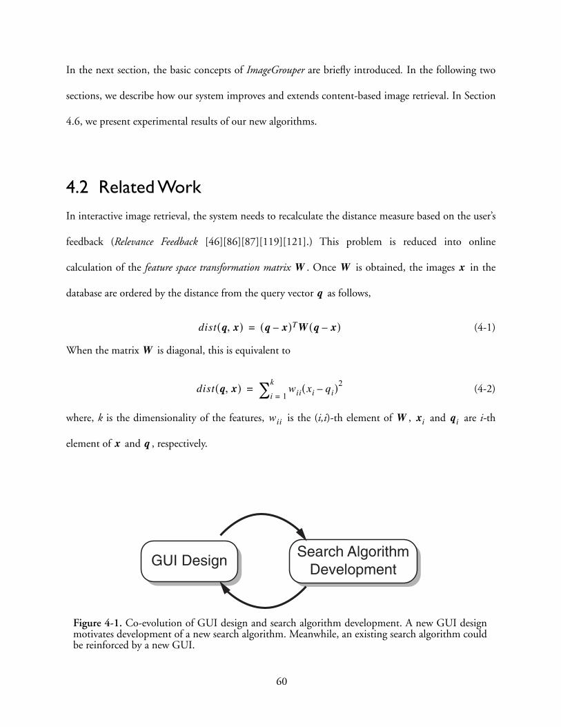
In the next section, the basic concepts of ImageGrouper are briefly introduced. In the following two
sections, we describe how our system improves and extends content-based image retrieval. In Section
4.6, we present experimental results of our new algorithms.
4.2 Related WorkIn interactive image retrieval, the system needs to recalculate the distance measure based on the user’s
feedback (Relevance Feedback [46][86][87][119][121].) This problem is reduced into online
calculation of the feature space transformation matrix . Once is obtained, the images in the
database are ordered by the distance from the query vector as follows,
(4-1)
When the matrix is diagonal, this is equivalent to
(4-2)
where, k is the dimensionality of the features, is the (i,i)-th element of , and are i-th
element of and , respectively.
GUI DesignSearch Algorithm
Development
Figure 4-1. Co-evolution of GUI design and search algorithm development. A new GUI designmotivates development of a new search algorithm. Meanwhile, an existing search algorithm couldbe reinforced by a new GUI.
W W x
q
dist q x,( ) q x–( )T W q x–( )=
W
dist q x,( ) wii xi qi–( )2
i 1=
k∑=
wii W xi qi
x q
60
In most methods discussed below, the query vector is defined as the weighted centroid of N positive
examples specified by the user:
(4-3)
where is the n-th positive example, and is its degree of relevance. Porkaew et al. [78][79]
proposed another way to define the query points. In their Query Expansion (QEX) method, multiple
query points are created by clustering relevant examples. The distance from each image in the database
to the multipoint query is the weighted combinations of the distance from the image to the centroid
of each query cluster. The weight for each query cluster is proportional to the number of relevant
examples in the cluster.
In the following subsections, we briefly explains previously proposed methods in the literature. Those
approaches can be classified into four types by the ways the system address the image retrieval:
• One-Class Relevance Feedback [46][86][87]
• Two-Class (positive and negative) Relevance Feedback [26][33]
• (1+x)-Class (one positive and x negatives) Relevance Feedback [119]
• Multi-Class Relevance Feedback [76]
4.2.1 Image Retrieval as a One-Class Problem
When no negative image examples are considered, the simplest way of feature weighting is to calculate
the variance of each feature among the query examples. First, the variance of each feature
among the positive examples (relevant images) is calculated. Then, the inverse of
q
qπnxnn 1=
N∑πnn 1=
N∑-----------------------------=
xn πn
σ1 σ2 σ3 … σk, , , ,( )
61
variance becomes the weight of each feature [86]. Thus, the feature weighting matrix becomes a
diagonal matrix:
(4-4)
where is the (i, i)-th element of W.
This gives higher weights to the features in which example images are similar. If the number of example
images is larger than the dimensionality of the features, the optimal solution of is proposed by Rui
et al. [87] as follows:
(4-5)
where k is the dimensionality of the features, and C is the weighted covariance matrix [46] of the
N positive examples defined as,
(4-6)
is the (i,i)-th element of , is the i-th element of n-th image in the database and is the
degree of the relevance for n-th image specified by the users (Chapter 3.) takes a full matrix form
when the number of relevant images are larger than the dimensionality of the features.
In [23], Chen et al. applied variants of Support Vector Machine [12][16][111] called (linear) One-class
SVM (LOC-SVM) and Kernel One-class SVM (KOC-SVM) [90] to the one-class image retrieval
problems. The authors reported that in their experiments with 500 images, KOC-SVM outperformed
LOC-SVM and the linear transform based approaches discussed above.
W
wii1σi-----=
wii
W
W det C( )( )1 k⁄ C 1–=
k k×
Cij πn xni qi–( ) xnj q j–( ) πnn 1=N∑( )⁄
n 1=N∑=
Cij C xni πn
W
62

4.2.2 Image Retrieval as a Two-Class Problem
Some systems allow the user to specify negative (irrelevant) examples explicitly. Therefore, image
retrieval can be considered as a two-class classification problem. One example of this problem is the
Fisher’s Discriminant Analysis (FDA) [26][33]. FDA tries to maximize the distance between the two
classes (between class scatter) while minimizing scatters within each class (within scatter.) The within-
scatter matrix is defined as follows,
(4-7)
and are the scatters of two classes ( and ) as follows,
(4-8)
where is the mean vector of a class . Next, the between-scatter matrix is defined as follows,
(4-9)
Finally, the criterion function of FDA is
(4-10)
Several researchers applied Support Vector Machine [12][16][111] to two-class image retrieval
[48][110][118]. In [110], Tong and Chang proposed an Active Learning method. During the relevance
feedback loops of this method, the system displays “the most informative” images instead of “the most
relevant” images. The users are then asked to select only relevant images from the image set. The images
to display are chosen so that the possible solution space (called version space) is halved after each
feedback.
SW S1 S2+=
S1 S2 C1 C2
Si x mi–( ) x mi–( )x Ci∈∑=
mi Ci
SB m1 m2–( ) m1 m2–( )T=
WWT SBW
WT SW W-----------------------
Wargmax=
63
Meanwhile, Wu et al. [117] applied Discriminant Expectation-Maximization (D-EM) algorithm to
image retrieval problem. The D-EM approach requires, however, many annotated data and
computationally expensive.
These systems are addressing image retrieval as a two-class (positive and negative) problem (Figure 4-2
(a).) These approaches, however, introduce undesirable side effects because they mix up all negative
examples into one class. In the actual scenario of image retrieval, negative examples can be from many
classes of images in the database.
4.2.3 Image Retrieval as a (1+x)-Class Problem
Zhou et. al. [119][121] proposed a new relevance feedback algorithm, which takes negative examples
into account effectively. They consider the relevance feedback problem as a (1+x)-class (i.e., one positive
and multiple negative classes) problem (Figure 4-2 (b).) In this scheme, it is assumed that the negative
examples are coming from an uncertain number of classes, while the positive examples can be clustered
into one class. Their algorithm, named Biased Discriminant Analysis (BDA) is characterized by the
following objective function,
(4-11)
where,
(4-12)
(4-13)
is a set of positive examples and D is a set of negative examples. In short, BDA tries to minimize
within-class scatter matrix of the positive example, while is keeping the negative examples
WWT SbiasW
WT SW W--------------------------W
argmax=
SW x m–( ) x m–( )Tx C∈∑=
Sbias x m–( ) x m–( )Ty D∈∑=
C
SW Sbias
64
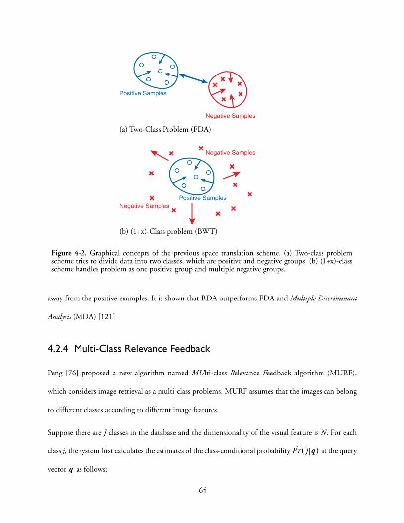
away from the positive examples. It is shown that BDA outperforms FDA and Multiple Discriminant
Analysis (MDA) [121]
4.2.4 Multi-Class Relevance Feedback
Peng [76] proposed a new algorithm named MUlti-class Relevance Feedback algorithm (MURF),
which considers image retrieval as a multi-class problems. MURF assumes that the images can belong
to different classes according to different image features.
Suppose there are J classes in the database and the dimensionality of the visual feature is N. For each
class j, the system first calculates the estimates of the class-conditional probability at the query
vector as follows:
Negative Samples
Positive SamplesNegative Samples
Positive Samples
Negative Samples
Figure 4-2. Graphical concepts of the previous space translation scheme. (a) Two-class problemscheme tries to divide data into two classes, which are positive and negative groups. (b) (1+x)-classscheme handles problem as one positive group and multiple negative groups.
(a) Two-Class Problem (FDA)
(b) (1+x)-Class problem (BWT)
Prˆ j q( )
q
65
(4-14)
Next, the system assumes that the images can be clustered differently for each dimension. Thus, it also
calculates the estimate of the class-conditional probability of the query vector attributed
to the i-th feature ( ),
(4-15)
The parameters to determine the neighbor (i.e., the number of neighbors) are defined by the users.
and are normalized as follows,
(4-16)
(4-17)
where,
(4-18)
(4-19)
and and are constants. Then, it calculates “the ability of i-th feature to predict the s at
” [76] for the weighted distance,
(4-20)
Here, becomes larger when the difference between class-conditional probability of the whole query
vector and that of its i-th feature is small. Therefore, it measures how much the i-th feature contributes
to the posterior probabilities. Finally, the feature weighting matrix becomes a diagonal matrix,
Prˆ j q( ) # of neighbors of the query that is labeled as class jTotal # of neighbors of the query
--------------------------------------------------------------------------------------------------------------------------=
Prˆ j xi qi=( )
i 1…k=
Prˆ j xi qi=( ) # of neighbors along the i th feature labeled as class j
Total # of neighbors along the i th feautre-------------------------------------------------------------------------------------------------------------------------------=
Prˆ j q( ) Prˆ j xi qi=( )
Pr˜ j q( ) Prˆ j q( ) c1 P̂ Prˆ j q( )–( )+=
Pr j xi qi=( ) Prˆ j xi qi=( ) c2 Piˆ Prˆ j xi qi=( )–( )+=
P̂1J--- Prˆ j q( )
j 1=
J∑=
P̂i1J--- Prˆ j xi qi=( )
j 1=
J∑=
c1 c2 Pr j q( )
qi zi= χ2
ri Pr j xi qi=( ) Pr˜ j q( ) Pr j xi qi=( )–[ ]2
j 1=
J∑=
ri
66
(4-21)
where
(4-22)
This means a feature with smaller is given a higher weight. These values have similar effect to Eq.
4-4, where more discriminating features are given higher weights and each feature is independent of
the others.
In theory, MURF can support arbitrary number of image classes and the author tested the system on
eight class classification on simulated data. Meanwhile, the system is also tested on real image retrieval
problems. Unlike our proposed system (Section 4.3,) however, the image retrieval is considered as a
three class problem where the users label the images as “relevant,” “somewhat relevant,” or “irrelevant.”
Since this method can be considered as a coarse way to specify the degree of relevance rather than a
multi-class classification, it can be classified as a variant of two-class classification problems discussed
in Section 4.2.2.
Peng claims the better retrieval performance of MURF [76] over his previous PFRL (Probabilistic
Feature Relevance Learning) system [75]. However, it might be because of more query examples. That
is in their experiments, MURF is given both “relevant” and “somewhat relevant” examples, while PFRL
is given only relevant examples [76].
wii
T ri( )exp
T rl( )expl 1=q∑
--------------------------------------=
ri r j{ }j
max ri–=
ri
67

4.3 Proposed Approach: Extending to a (x+y)-Class ProblemIn the initial version of ImageGrouper (Chapter 3), when the user specifies more than one group as
positive, these groups are merged into one group for a query. Thus, Biased Discriminant Analysis
described in Section 4.2.3 was used to calculate the feature weights. Here, the system supported one
positive group and multiple negative groups.
However, this approach is not taking full advantages of our group-oriented interface. When the user
searches images, s/he may have high-level concepts in her/his mind such as “beautiful flowers.” Such
concepts cannot be expressed by only one class of images. See Figure 4-3. Although white flowers and
red flowers may have common visual features, they also have very different features, which are the color
features. If the system tries to put them together as one class of images, the color features have to be
discarded. This is not desirable because these features may be beneficial to retrieve a specific color of
flowers.
Figure 4-3. White flowers and Red flowers. Both groups can be considered as subsetsof “flower class” In ImageGrouper, users can separate them into two positive groups.
White Flowers Red Flowers
Flowers
68

For the users, it is more intuitive if they can specify them as two different, but closely related subsets
of an image class. This problem has not been addressed before because the traditional user interfaces
do not allow the user to divide positive image examples into multiple groups. This fact motivated us
to extend the relevance feedback problems to a (x+y)-class (i.e. multiple positive and multiple negative
classes) problem.
In our new scheme, named Group Biased Discriminant Analysis (GBDA), the objective function is:
(4-23)
where is the sum of the within-class scatter matrix [26] of the positive groups as defined as follows,
(4-24)
(4-25)
where, is the mean vector of i-th positive class , and c is the number of samples in the group.
is the positive-to-negative scatter, which is introduced in this chapter as follows,
(4-26)
(4-27)
where, is the set of the negative examples.
Figure 4-4 illustrates the concept of our scheme. In short, GBDA tries to cluster each positive class
while trying to scatter the negative examples away from the positive classes. Like BDA, each negative
example belongs to its own class.
As in FDA and BDA, is solved as the generalized eigenvector(s) associated with the largest
eigenvalue(s) ,
WWT SPNW
WT SW W-------------------------
Wargmax=
SW
SW Sii 1=c∑=
Si x mi–( ) x mi–( )Tx Ci∈∑=
mi Ci
SPN
SPN SNii 1=c∑=
SNi y mi–( ) y mi–( )Ty D∈∑=
D
W
λ
69
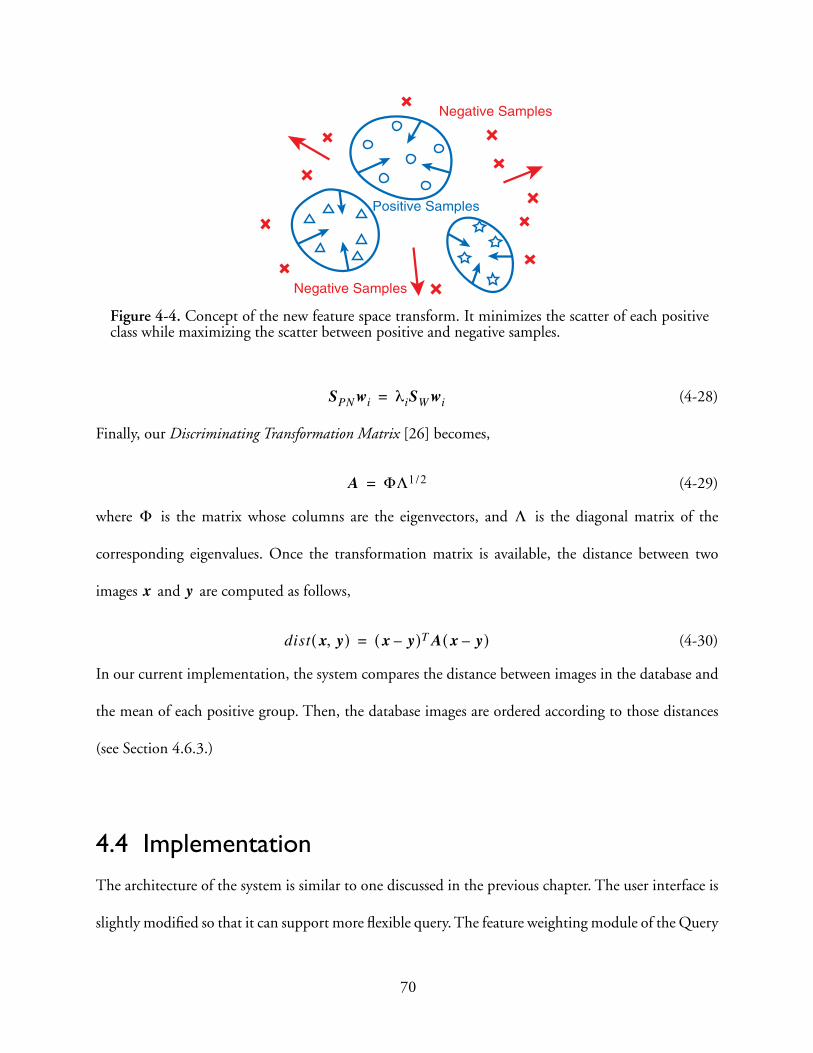
(4-28)
Finally, our Discriminating Transformation Matrix [26] becomes,
(4-29)
where is the matrix whose columns are the eigenvectors, and is the diagonal matrix of the
corresponding eigenvalues. Once the transformation matrix is available, the distance between two
images and are computed as follows,
(4-30)
In our current implementation, the system compares the distance between images in the database and
the mean of each positive group. Then, the database images are ordered according to those distances
(see Section 4.6.3.)
4.4 ImplementationThe architecture of the system is similar to one discussed in the previous chapter. The user interface is
slightly modified so that it can support more flexible query. The feature weighting module of the Query
SPNwi λiSW wi=
A ΦΛ1 2/=
Φ Λ
Negative Samples
Positive Samples
Negative Samples
Figure 4-4. Concept of the new feature space transform. It minimizes the scatter of each positiveclass while maximizing the scatter between positive and negative samples.
x y
dist x y,( ) x y–( )T A x y–( )=
70

Server is replaced with the new algorithms. When the user does not specify any negative examples, the
server use Multiple Discriminant Analysis (MDA) [26] instead of GBDA. Currently, the system runs on
Solaris, Mac OS X, and Microsoft Windows. They are implemented in Java and C++ with CLAPACK
[2] and Automatically Tuned Linear Algebra Software (ATLAS) [4]. The Windows version requires
Cygwin [80] to compile. For the Solaris version, Sun Performance Library [106] is used instead of
ATLAS. In addition, we also implemented this algorithm on MATLAB. The MATLAB version of our
algorithm made modification and evaluation of our algorithms easier. Experiments discussed in the
following section are conducted with this version.
4.5 Analysis on Toy ProblemsTo illustrate the effects of GBDA, we use three-dimensional toy problems as shown in Figure 4-5 and
Figure 4-6. The original data are plotted in 3D where the positive examples are represented by ‘o’s and
negative ones by ‘x’s. The projections of the data into a two-dimensional space are shown directly below.
In this section, we address two typical cases. The first case is when two positive clusters are distant from
each other (Figure 4-5.) The second case is when two positive clusters are close to each other (Figure 4-
6.) In both cases, the negative examples are scattered across the problem space. We compared the
projection results with Multiple Discriminant Analysis (MDA) [26] and BDA. In MDA, the negative
examples are considered as one class. Thus, it deals with the problem as a three-class (two positive and
one negative) one.
In the first case, BDA merges the two positive clusters into one while MDA and GBDA preserve the
separation of the two clusters. GBDA clusters each positive class tighter than MDA. For the second
case, GBDA and BDA have similar effects: the two positive clusters are merged into one positive
71
cluster. This is a desirable effect since these two positive groups are very close to each other and should
be considered as one group even though the user specifies them as different. Meanwhile, although
MDA keeps these positive groups separated, it attracts the negative examples towards one positive
cluster. This effect is not suitable for image retrieval since it increases the possibility that many
irrelevant images are retrieved.
4.6 Experiments on Real Data
4.6.1 Data Sets
To examine the advantages of GBDA over BDA, the retrieval performances of the two systems are
tested on COREL image database. The dimensionality of the image feature space (color, texture and
structure) is 37 as described in the previous chapters. We used a subset of 804 images from the database.
These subset images consisted of six classes of images: airplanes, cars, flowers, stained-glass, horses and
eagles. From each class, up to 40 images are given as positive query examples. For GBDA, the query
examples are further divided into two sub-groups by the domain expert. For example, images of horses
are divided into two subsets: “white horses” and “brown horses.” In BDA, they are considered as one
group. For simplicity, the sizes of the sub-groups are kept the same (up to 20.) Figure 4-7 shows the
images from two representative test sets. The first set (Figure 4-7 (a)) is images of “Horses.” The image
set is divided into two subsets: “white horses and brown horses.” The second set is images of “Flowers.”
They are also divided into two subsets: “red flowers” and “yellow flowers.”
72
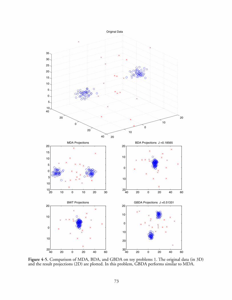
20
10
0
10
20
40
20
0
20
40 10
5
0
5
10
15
20
25
30
35
Original Data
20 10 0 10 20 30 15
10
5
0
5
10
15
20MDA Projections
40 20 0 20 40 60 20
10
0
10
20BDA Projections J =0.18565
40 20 0 20 40 60 20
10
0
10
20BWT Projections
40 20 0 20 40 60 30
20
10
0
10
20GBDA Projections J =0.51331
Figure 4-5. Comparison of MDA, BDA, and GBDA on toy problems 1. The original data (in 3D)and the result projections (2D) are plotted. In this problem, GBDA performs similar to MDA.
73

20 10 0 10 20 20
10
0
10
20
30MDA Projections
40 20 0 20 40 60 30
20
10
0
10
20BDA Projections J =0.70149
40 20 0 20 40 60 30
20
10
0
10
20BWT Projections
40 20 0 20 40 40
30
20
10
0
10
20GBDA Projections J =0.75454
20
10
0
10
20
40
20
0
20
40 10
5
0
5
10
15
20
25
30
35
Original Data
Figure 4-6. Comparison of MDA, BDA, and GBDA on toy problems 2. The original data (in 3D)and the result projections (2D) are plotted. In this toy problem, GBDA performs similarly to BDA.
74

Figure 4-8 (a) and (b) shows the result of the two images classes. For each test, an equal number of
images are picked from the sub-group. Therefore, the total sample size is varied from 2 to 40 (in
increments of two.)
4.6.2 Performance Measures
As a performance measure, we introduced the weighted hit count. The weighted hit count (whc) is
calculated as follows. For each image in the top 20 results,
(4-31)
where,
(4-32)
and is the target image class. In this scheme, every relevant image in the result set is given a count
of one. Meanwhile, any false hits are given negative points based on their ranks in the result set.
Therefore, false hits that are closer to the top of the list are penalized more than those at the bottom of
the list. This measure reflects the quality of returned ranking as well as the number of correctly returned
images. We conducted each test 10 times and the results are averaged.
4.6.3 Ranking Strategies for GBDA
For GBDA, we used two different ranking strategies (GBDA-1 and GBDA-2.) For both strategies, two
different ranking are calculated based on the distance from the two group means. Then, GBDA-1
returns the top 10 images from each group. On the other hand, GBDA-2 orders the images by the
closer of the distances to one of the two groups and the top 20 images are returned.
xi
whc hc xi( )i 1=20∑=
hc xi( )1 xi C∈( )
1 i⁄ (otherwise)–⎩⎨⎧
=
C
75

Figure 4-7. Sample Query Images. Each set is divided into two sub-sets.
(a) Horses
(b) Flowers
76

4.6.4 Results
Figure 4-8 (a) and (b) shows the result of “horses” and “flowers” respectively. The horizontal axis is the
number of positive examples. The vertical axis is the weighted hit count described above.
In the case of “horses” (Figure 4-8 (a)), when the number of query examples is small (sample size < 8),
GBDA-1 shows similar performance as BDA. GBDA-2 performs worse than BDA.
When the number of samples gets larger (sample size > 8), GBDA-1 performs better than BDA, while
GBDA-2 shows similar performance as BDA. This corresponds to the first toy problem in Section 4.5.
It also shows that in order for GBDA to take advantages of the group information, it requires at least
four samples from each group.
Figure 4-8 (b) shows the results of “red and yellow flower” images. In this case, there are no significant
differences among BDA, GBDA-1 and GBDA-2. This is because the two groups are too close to each
other1 for GBDA to create two separated clusters. Note that GBDA does not do any harm even if it
cannot utilize group information. In this situation, it has similar effects as BDA. This corresponds to
the second toy problem.
Figure 4-9 (a) and (b) show the same results in the precision and recall [5] for different sample sizes.
Recall and precision are defined as follows:
(4-33)
(4-34)
1. The closeness of two groups depends on the diversity of images in the database.
RecallThe number of relevant images retrieved
The number of relevant images in the database----------------------------------------------------------------------------------------------------------------=
PrecisionThe number of relevant images retrieved
The number of retrieved images -------------------------------------------------------------------------------------------------=
77

0 2 4 6 8 10 12 14 16 18 2015.5
16
16.5
17
17.5
18
18.5
19
19.5
20HORSES
Sample Size / 2
# H
its (
on w
eigh
ted
aver
age)
GBDA 1 * 19.105
GBDA 2 * 18.455
BDA * 18.615
0 2 4 6 8 10 12 14 16 18 207
7.5
8
8.5
9
9.5
10
10.5
11
11.5
Sample Size / 2
# H
its (
on w
eigh
ted
aver
age)
FLOWERS
GBDA 2 - 8.725
BDA - 8.975
GBDA 1 - 9.04
Figure 4-8. Comparison of BDA and GBDA on the real data. The results are shown in theweighted hit count.
(a) Horse Examples
(b) Flower Examples
78
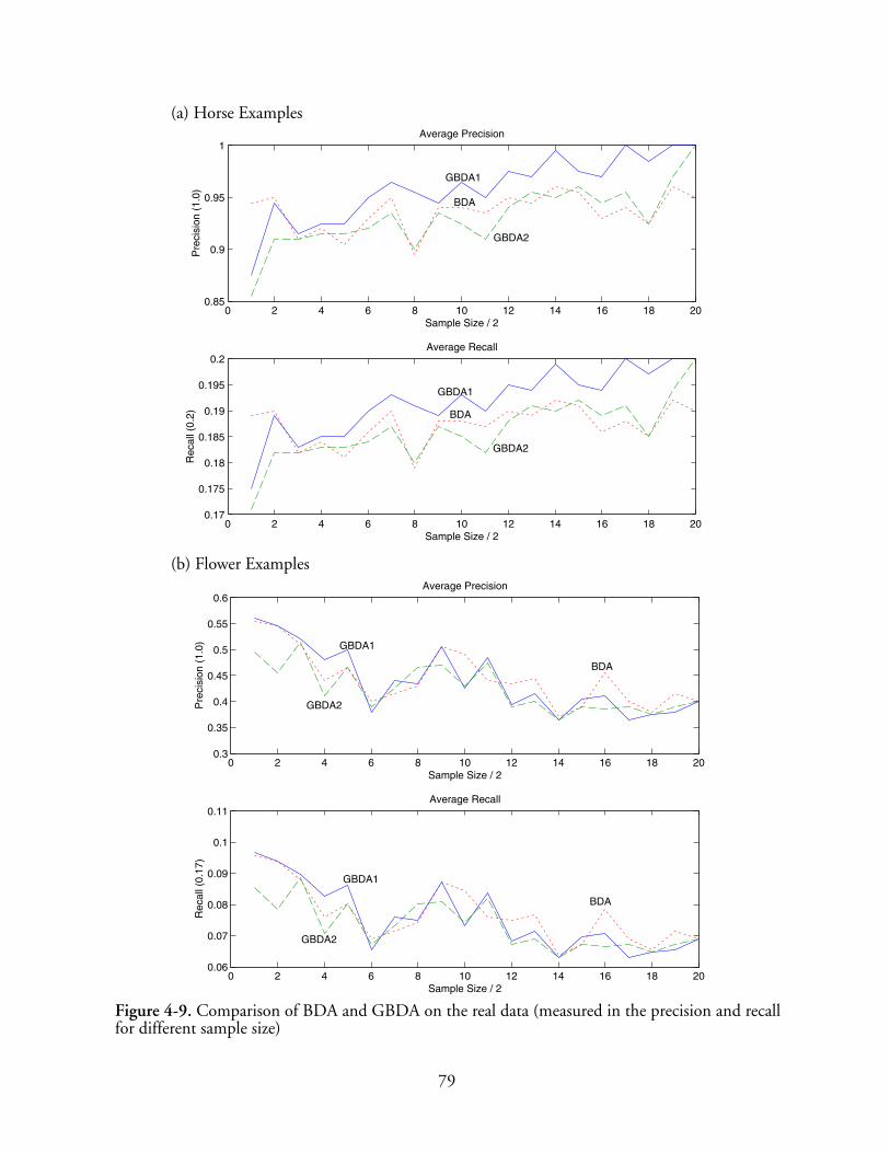
0 2 4 6 8 10 12 14 16 18 200.85
0.9
0.95
1Average Precision
Sample Size / 2
Pre
cisi
on (
1.0)
0 2 4 6 8 10 12 14 16 18 200.17
0.175
0.18
0.185
0.19
0.195
0.2Average Recall
Sample Size / 2
Rec
all (
0.2)
GBDA1
BDA
GBDA2
GBDA1
BDA
GBDA2
0 2 4 6 8 10 12 14 16 18 200.3
0.35
0.4
0.45
0.5
0.55
0.6Average Precision
Sample Size / 2
Pre
cisi
on (
1.0)
0 2 4 6 8 10 12 14 16 18 200.06
0.07
0.08
0.09
0.1
0.11Average Recall
Sample Size / 2
Rec
all (
0.17
)
GBDA1
GBDA1
GBDA2
GBDA2
BDA
BDA
Figure 4-9. Comparison of BDA and GBDA on the real data (measured in the precision and recallfor different sample size)
(a) Horse Examples
(b) Flower Examples
79

Note that in information retrieval with relevance feedback, many systems include the query examples
themselves in the query result so that the user can reuse the images in the previous query. Therefore,
the traditional Precision versus Recall curve [5] is not suitable for the evaluation.
4.7 ConclusionWe are investigating query algorithms that can take advantage of the group-oriented user interface. In
this chapter, we introduced a new feature space transform algorithm. In this method, the user’s interest
can be expressed as a (x+y)-class (multiple positive and multiple negative) problem. This new scheme
is inspired by the development of the user interface. In fact, there was no way to apply this scheme on
the traditional interfaces because the user could not specify positive examples as multiple classes.
4.8 Possible Improvement
4.8.1 Groups with Different Sizes
In our experiments, we assumed that the sizes of two positive groups are equal. This is not appropriate
assumption in the real world. Especially with relevance feedback, the user adds new images into the
groups. Therefore, it is very likely the number of image in each group is different. We will investigate
the case of different group sizes. It may be necessary to normalize the clusters to prevent the returned
result from being biased to the larger group.
80

4.8.2 Automated Clustering of Groups
Although making groups on ImageGrouper is very easy, it would be convenient if the system can
automatically create multiple positive groups from one positive group. Once groups are created, this
group information can be used by GBDA. While this approach gives less control to the users, it can
avoid making superfluous groups.
4.8.3 More than Two Groups
In this chapter, we used only two positive groups. Although our implementation supports an arbitrary
number of positive groups, the benefit of more than two groups is not clear. In order to determine the
properties of each group, the system requires several samples for each group. Unless plenty of positive
examples are available, it is difficult to create many groups effectively.
81

Chapter 5
Integrating ImageGrouper into the 3D Virtual Space
5.1 IntroductionIn the previous chapters, we introduced two different types of user interface for content-based image
retrieval: 3D MARS and ImageGrouper. Both systems have their own strength and weakness. Table 5-
1 compares 3D MARS and ImageGrouper in various aspects. Here, we assume 3D MARS is used in a
projection based virtual reality system (i.e., CAVE see Figure 2-2 on page 14.) 3D MARS can display
many images simultaneously in the three-dimensional virtual reality space. Therefore, it is suitable for
finding relevant images from many irrelevant images. In addition, those images are located based on
three different criteria along x, y, and z axis. Therefore, it provides a powerful visualization tool for the
visual feature space.
However, because the electromagnetic tracking devices attached on the wand and shutter glasses
(Section 2.5) are not very accurate. Moreover, because the immersive 3D virtual reality is realized by
projecting images on the four flat screens, the objects can not be perfectly aligned. As a result, there are
discrepancies between the tracking and the 3D projection. Thus, it is very difficult for the user to
conduct operations that require precision in CAVE. Interactions are limited to simple operations such
82

as touching and moving relatively large objects. It is not suitable for manipulating small objects. Hence,
the user of 3D MARS creates a query by touching the images and clicking the wand button as discussed
in Section 2.5. S/he can only specify each image as relevant, irrelevant or neutral. Furthermore, since
the images are scattered in the space, grouping operation is not straightforward. The user has to fly
though the space to collect images with a joystick.
Meanwhile, ImageGrouper uses a mouse as an input device. Therefore, it can support finer and more
accurate control on the workspace. In addition, the user can make a flexible query by making image
groups. On the other hand, the workspace is two-dimensional. Thus, it can display only a limited
number of images at the same time.
We are interested in how we can take advantages of ImageGrouper and 3D MARS by integrating the
two systems. In the following sections, we discuss the design choices of the integration, the system
architecture, and the benefit of the integration.
Table 5-1. Comparison of 3DMARS and ImageGrouper
3DMARS ImageGrouper
Display Dimensionality 3D 2D
Number of images to be displayed Many Limited
Control Device Wand Mouse
Control Accuracy Inaccurate Accurate
Flexibility of Query Less Flexible (only rele-vant and irrelevant)
Flexible(Query-by-Groups)
83

5.2 Design ChoicesFor integration, we had two choices. The first option was to realized the group-oriented interaction
similar to ImageGrouper in CAVE. The second option was to bring a wireless equipped portable device
that runs ImageGrouper into CAVE.
Although implementing the first method is easy, grouping operation in this method is awkward for
several reasons. First, grouping operation requires enclosing objects in the three-dimensional space. In
the case of 3D MARS in CAVE, this can be achieved by allowing the user to draw a translucent
rectangular solid that encloses images. However, since the images are flat rectangle plates, it is hard for
the user to see whether an image is within the rectangular solid. In addition, as discussed above, the
images in 3D MARS are scattered in the space. To enclose many images, the user has to draw a large
rectangular solid or put relevant images together by flying through the space.
Therefore, we chose the second option, i.e., to bring a portable device running ImageGrouper into
CAVE. In the next section, we discuss how the users interacts with the integrated system for image
retrieval tasks.
5.3 User Interaction of Grouper in 3D MARSFigure 5-1 shows a user interacting with ImageGrouper in 3D MARS. The user is holding a wireless
equipped notebook PC, which is running a customized version of ImageGrouper. This version of
ImageGrouper is designed to synchronize with 3D MARS as described in the next section. Ideally,
tablet-based PCs or PDAs should be used because the user has to hold the device in CAVE. Pen input
is a natural choice for drag-and-drop operation in the group-oriented user interactions in this situation.
84

In the integrated system, ImageGrouper and 3D MARS are always synchronized. Both systems display
the same set of images. This means 3D MARS displays all images that appear in both the GroupPalette
and the ResultView of the ImageGrouper (Section 3.3.) The images’ locations in the 3D space are
determined by their visual features.
The user interactions are also synchronized. When the user selects an image on ImageGrouper, the same
image in 3D MARS is highlighted and vice versa. If an image clicked in 3D MARS is hidden in the
ResultView of ImageGrouper, it automatically scrolls so that the image is visible. If the user delete an
image in one user interface, the same image disappears in the other interface. When the user clicks a
group in the GroupPalette, all images in the group are highlighted simultaneously in 3D MARS. Thus,
the user can see how images in the group s/he created are distributed in the feature space. In addition,
the user can change the display options of 3D MARS such as the sphere mode (Section 2.5) and the
Figure 5-1. User interacting in 3DMARS with a wireless-equipped note book PC.
85

projection strategies (Section 2.8.1) from menus of ImageGrouper. The user does not have to touch the
buttons in the 3D space.
The user can create a query from either system. The query method differs depending on the system on
which the user creates the query. Query in ImageGrouper is the Query-by-Groups method where the
user can specify an arbitrary number of image groups (Section 3.3.) As described above, this Query-
by-Group operation is difficult in 3D MARS. Therefore, query in 3D MARS is the standard Query-by-
Example method where the user specifies images as relevant, irrelevant or neutral. Regardless of system
the query is created, the search results are displayed on both systems.
5.4 System ArchitectureFigure 5-2 show the system architecture of the Grouper in 3D MARS system. The portable device in
CAVE is running a customized version of ImageGrouper. This version is designed to control and
synchronized with the 3D MARS. The device is equipped with IEEE 802.11b wireless card so that it
can communicate with 3D MARS and the Query Engine without a wire. When the user presses the
query button on the grouper, the grouper sends a query to the Query Engine. In addition to the IDs
and files names of the result images, this version receives the feature distances from the query vector of
the images. The grouper not only displays the results on its ResultView, but also sends those
information to 3D MARS. Then, 3D MARS loads the image files directly from the Query Engine.
When the user makes a query and presses the button from 3D MARS, the system collects query
information in the 3D space and sends it to ImageGrouper. Then, ImageGrouper sends the query to the
Query Engine, receives the result, and forward it to 3D MARS. Therefore, 3D MARS communicates
86
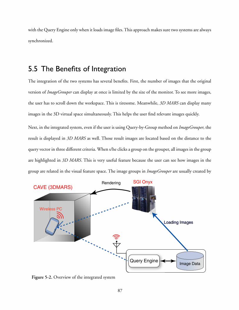
with the Query Engine only when it loads image files. This approach makes sure two systems are always
synchronized.
5.5 The Benefits of IntegrationThe integration of the two systems has several benefits. First, the number of images that the original
version of ImageGrouper can display at once is limited by the size of the monitor. To see more images,
the user has to scroll down the workspace. This is tiresome. Meanwhile, 3D MARS can display many
images in the 3D virtual space simultaneously. This helps the user find relevant images quickly.
Next, in the integrated system, even if the user is using Query-by-Group method on ImageGrouper, the
result is displayed in 3D MARS as well. Those result images are located based on the distance to the
query vector in three different criteria. When s/he clicks a group on the grouper, all images in the group
are highlighted in 3D MARS. This is very useful feature because the user can see how images in the
group are related in the visual feature space. The image groups in ImageGrouper are usually created by
CAVE (3DMARS)SGI Onyx
Image Data
Loading ImagesLoading Images
Wireless PC
Rendering
Query Engine
Figure 5-2. Overview of the integrated system
87

the user based on his/her high level semantic concepts. Therefore, the images in the group are not
necessarily close to one another in the feature space. Visualizing image groups in the 3D feature space
helps effective trial-and-error query. If one of images in a group is located far from the others (i.e.,
outlier) removing this image may improve the query result. Finding those outliers in two-dimensional
user interfaces is very difficult.
88
Chapter 6
Storage and Visual Features for Content-based Image Retrieval
In this chapter, we discuss additional research topics we are investigating. The first topic is data
structures for high-dimensional data. The second topic is feature extraction of local image features. In
addition, we discuss integration of text information with low-level image features.
6.1 Data Structure for High-Dimensional Data Access
6.1.1 Background
Content-based Image Retrieval (CBIR) systems need to store the metadata of the image files on the
disks. Those meta-data are numerical, and high-dimensional data made of low-level visual features
(Appendix A) It is difficult to manage these data with traditional commercial database systems because
these systems are designed for text and low-dimensional numerical data. Thus, many researchers have
proposed architectures for indexing high-dimensional data [10][11][12][35][38][50]
[57][81][88][113][114]. Some systems index numerical data into B-tree like hierarchical structures
[8][10][38]. Other systems separate data space into grid regions and construct a tree of the regions
89
[72][81][81][92]. Most of the systems were designed to minimize the number of I/O access to the
disks.
Few researchers, however, take the real time performance into account. Therefore, many systems
consume an enormous amount of computation (CPU time) in creating and traversing complicated
trees while they are minimizing I/O accesses time. Beyer et. al. [13] showed that in high (10-15)
dimension, a simple linear scan algorithm outperforms those sophisticated index structures. This is
because many sophisticated data structures do not scale to larger dimensionality. When the
dimensionality gets higher, those systems have to traverse every node in the trees. Meanwhile, the linear
scan requires a minimal number of computation in any dimensionality. Therefore, Beyer et. al.
recommend every researcher compare his/her new algorithms with the linear scan [13].
The advantages of linear scan increase dramatically when the size of memory gets larger because the
linear scan can utilize as much memory as available for caching the data in the disks. These days, the
price of memory is getting lower. Therefore, it is very difficult to exceed the speed of the linear scan.
Weber et. al. [113] proposed an approximation-based data structure named VA-File. In VA-File, each
datum on the disks is quantized into 4-6 bits per dimension. These data are used as an approximation
to the original data. Because the size of the quantized data is much smaller, the system can hold all
approximated data in the main memory. For the nearest neighbor query, the system first scans every
approximated datum on memory and finds candidate data. Then it loads only data block where the
candidate data are stored. Because many data are pruned in the first phase, it reduces I/O accesses in
the second phase. In addition, it requires only a small amount of computation since it does not create
a complicated data structure. Wu and Manjunath applied VA-File to interactive image retrieval systems
[116].
90

While VA-File is very simple and outperforms the other sophisticated methods, it cannot utilize a large
memory space. The size of approximated memory is proportional to the number of data in the original
database. Therefore, even if more memory is available, VA-File cannot improve the search time further.
As a result, when a large amount of memory is available and the dimensionality is large, the linear scan
algorithm still outperforms VA-File [22]. In addition, because the approximated data are squeezed into
smaller region, each datum is not aligned in byte boundaries. Thus, the system requires many memory
copy operations for various computation.
6.2 Preliminary ExperimentsWe are investigating new algorithms to overcome the bottleneck of VA-File [22]. First, we have
implemented “cache-aware” versions of X-Tree [10], VA-File and the linear scan algorithm [22]. These
customized versions are designed to utilize the available memory as much as possible. For example, our
new implementation of X-Tree caches data blocks and superblocks in memory. These improvements
are very important especially when relevance feedback is used for data retrieval. During relevance
feedback loops, the same data are repeatedly accessed.
Then we compared real time performances of K-Nearest Neighbor search. Figure 6-1 shows the result
of our preliminary experiments. Here, K=50, Dimemsion=37 and the data size is 100,000 (it occupies
28MB of the disk.) The horizontal axis is the size of memory available, and the vertical axis is the time
required for K-Nearest Neighbor search. As shown in the figure, while the linear scan algorithm can
consistently improve the performance as the memory size increases, the performances of X-Tree and
VA-File are not improved. Therefore, when the available memory is small, VA-File outperforms the
scan. However, with larger memory, the scan searches faster than VA-File.
91
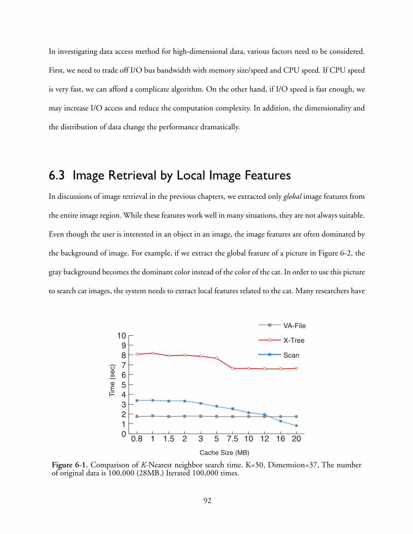
In investigating data access method for high-dimensional data, various factors need to be considered.
First, we need to trade off I/O bus bandwidth with memory size/speed and CPU speed. If CPU speed
is very fast, we can afford a complicate algorithm. On the other hand, if I/O speed is fast enough, we
may increase I/O access and reduce the computation complexity. In addition, the dimensionality and
the distribution of data change the performance dramatically.
6.3 Image Retrieval by Local Image FeaturesIn discussions of image retrieval in the previous chapters, we extracted only global image features from
the entire image region. While these features work well in many situations, they are not always suitable.
Even though the user is interested in an object in an image, the image features are often dominated by
the background of image. For example, if we extract the global feature of a picture in Figure 6-2, the
gray background becomes the dominant color instead of the color of the cat. In order to use this picture
to search cat images, the system needs to extract local features related to the cat. Many researchers have
0123456789
10VA-File
X-Tree
Scan
201612107.55321.510.8
Cache Size (MB)
Tim
e (s
ec)
Figure 6-1. Comparison of K-Nearest neighbor search time. K=50, Dimemsion=37, The numberof original data is 100,000 (28MB.) Iterated 100,000 times.
92

proposed image retrieval systems with local image features [18][19][28][98][102][116]. Most popular
approach is to extract features of objects by image segmentation [18][19][28][116]. For example,
Blobworld [18][19] ask the user to select his/her interested region from pre-segmented images. The
system extracts blobs from an image based on color and texture similarity and then calculates the
features of each blobs.
While those segmentation based approaches are very effective and intuitive for the users, there are
several drawbacks. First, although image segmentations are done off line, segmentation and feature
extraction on a large image database is prohibitive. Since the number of segments in each image differs,
search in the database is inefficient. Finally, image segmentation is not very robust and unreliable.
We are investigating simpler and more efficient ways of image retrieval with local image features. In
our approach, each image is divided into 5 by 5 grids. Then, image features for each grid are calculated
(Figure 6-2.) For retrieval, the system asks the user to select his/her interest by selecting a region of an
Figure 6-2. Block based image selection. In this example, the image is divided into 5 x 5 blocks.The user may be interested in region of 2 x 2 colored blue.
93

image by selecting the corresponding grids. In the case of Figure 6-2, the user selected 2 by 2 blocks
that enclose the cat (blue region.) The system approximates image features of this 2 by 2 region from
the features of blocks in this region (Figure 6-3.) In searching similar images in the database, the system
scans blocks of the same size. In this example, each image has 16 possible regions of 2 by 2 grids.
Smith et. al. [98] proposed similar approach for texture features. In their system, images are
decomposed into quad-tree structures (Figure 6-4.) For each node of the quad-tree, wavelet transform
is applied to extract local texture features. This system, however, searches only the same grid position
in the database. Thus, it cannot deal with translated images.
6.4 Integration of Content-based and Keyword-based Image RetrievalDespite the advances in content-based image retrieval research, the use of keyword information is very
helpful. “Annotation by Groups” method of ImageGrouper (Section 3.6 in Chapter ) makes it easier to
annotate keywords on many images. It also allows the user to create a semantic hierarchy of images.
F33 F34
F43 F44
F'
Figure 6-3. Approximating image region from smaller blocks.
94

MPEG-7 data types [62] allow text annotation to be attached on multimedia objects. The standard
supports various forms of text information including keywords, free text, structured annotation and so
on [62]. Figure 6-5 shows example of text annotation (keywords and free text.) These textural
information is stored in Extensible Markup Language (XML.) Because these information is stored with
multimedia contents descriptors, integration of content-based search and keyword-based search is
desirable.
Zhou et. al. [122] proposed a primitive system for integrated retrieval. In their system, keyword
information is integrated into low-level feature vectors. In the extended feature vectors, each keyword
Wavelet Transform
Original Image
Figure 6-4. Quad-Tree Decomposition [98].
<TextAnnotation><KeywordAnnotation>
<Keyword>Italy</Keyword><Keyword>Cat</Keyword><Keyword>Water</Keyword>
</KeywordAnnotation><FreeTextAnnotation xml:lang=”en”>
A cat is drinking water from a tap.Taken in Vernazza, Italy in 2002.
</FreeTextAnnotation></TextAnnotation>
Figure 6-5. Example of Keyword and Free Text Annotation of MPEG-7
95

is represented in a binary number that shows the existence of the keyword in an image. Therefore, the
dimensionality of the feature vector is “the dimensionality of the low-level features + the number of
keywords supported.” However, the system is not scalable because the number of keyword has to be
fixed. It also associates relationship between keywords only from low-level visual features without the
domain knowledge.
We will explore this problem further. We need to incorporate techniques of Text information retrieval
[5] and Data Mining [39] into content-based image retrieval systems.
96

Bibliography
[1] ACD Systems. “ACDSee” http://www.acdsystems.com.
[2] Anderson, E. et. al., “LAPACK Users' Guide,” Third Edition, Society for Industrial andApplied Mathematics, 1999.
[3] Apple Computer Inc. “iPhoto” http://www.apple.com/iphoto.
[4] Automatically Tuned Linear Algebra Software (ATLAS), http://math-atlas.sourceforge.net.
[5] Baeza-Yates, R. and Ribeiro-Neto, B. “Modern Information Retrieval.” Addison Wesley, 1999.
[6] Balabanovic, M., Chu, L.L. and Wolff, G.J. “Storytelling with Digital Photographs.” InCHI’00, 2000.
[7] Bates, M.J. “The design of browsing and berrypicking techniques for the on-line search inter-face.” Online Review, 13(5), pp. 407-431, 1989.
[8] Beckman, N., Kriegel, H.P., Schnneider, R. and Seeger, B., “The R*-Tree: An Efficient andRobust Access Method for Points and Rectangles,” In Proceedings of the ACM SIGMOD’90,1990.
[9] Bederson, B. B. “Quantum Treemaps and Bubblemaps for a Zoomable Image Browser.” HCILTech Report #2001-10, University of Maryland, College Park, MD 20742.
[10] Berchtold, S., Keim, D. and Kriegel, H-P., “The X-Tree: An Index Structure for High Dimen-sional Data.” In the 22nd VLDB Conference, 1996.
[11] Berchtold, S., Böhm, C., Jagadish, H.V., Kriegel, H-P. and Sander, J., “Independent Quantiza-tion: An Index Compression Technique for High-Dimensional Data Space,” In Proceedings ofICDE’00, 2000.
[12] Bernhard, E., Boser, I.G. and Vapnik, V., “A training algorithms for optimal margin classifiers,”In Proceedings of the 4th Workshop on Computational Learning Theory, pp. 144-152, San Mateo,CA, 1992.
97
[13] Beyer, K., Goldstein, J., Rmarkrishnan, R. and Shaft, U., “When Is “Nearest Neighbor” Mean-ingful?” In Proceeding of International Conference on Database Theory (ICDT’99), 1999.
[14] Brinkhoff, T., Kriegel, H-P., Schneider, R. and Seeer, B., “Multi-step Processing of SpatialJoins.” In SIGMOD Record (ACM Special Interest Group on Management of Data,) 23(2) 197-208, June 1994.
[15] Brown, M. H. and Hershberger, J., “Color and Sound in Algorithm Animation.” In IEEEComputer, Vol. 25, No. 12, December 1992.
[16] Burges, C., “A tutorial on support vector machines for pattern recognition,” In Data Miningand Knowledge Discovery, 2, pp.121-167, 1998.
[17] Card, S. K., Macinlay, J. D. and Shneiderman, B., “Readings in Information Visualization -Using Vision to Think,” Morgan Kaufmann, 1999.
[18] Carson, C. et. al., “Region-based Image Querying,” In Proceedings of IEEE Workshop onCBAIVL, June, 1997.
[19] Carson, C., Thomas, M. and Belongie, S., “Blobworld: A system for region -based image index-ing and retrieval,” University of California at Berkeley, 1999.
[20] Chen, J-Y., Bouman, C.A., and Dalton, J.C., “Heretical Browsing and Search of Large ImageDatabase,” In IEEE Transaction on Image Processing, Vol. 9, No. 3, pp. 442-455, March 2000.
[21] Chen, C., Gagaudakis, G. and Rosin, P., “Content-Based Image Visualization,” In Proceedingsof IEEE International Conference on Information Visualization (IV’00), 2000.
[22] Chen, T., Nakazato, M., and Huang, T. S., “Speeding up the Similarity Search in MultimediaDatabase.” In Proceedings of IEEE ICME2002, August, 2002.
[23] Chen, Y., Zhou, X. S. and Huang, T. S., “One-Class SVM for learning in image retrieval,” InProceedings of IEEE International Conference on Image Processing (ICIP’01), 2001.
[24] Cousins, S. B., et al. The Digital Library Integrated Task Environment (DLITE). In Proceedingsof 2nd ACM International Conference on Digital Libraries, 1997.
[25] Cox, I. J., Miller, M. L., Minka, T. P., Papathomas, T. V. and Yianilos, P. N. The Bayesian ImageRetrieval System, PicHunter: Theory, Implementation, and Psychophysical Experiments. InIEEE Transactions on Image Processing, Vol. 9, No. 1, January 2000.
[26] Duda, O. R., Hart, P. E. and Stork, D. G., “Patter Classification Second Edition”, Wiley-Inter-science, 2001.
98

[27] Faloutsos, C. and Ling, K., “FastMap: A Fast Algorithm for Indexing, Data-Mining and Visual-ization of Traditional and Multimedia Datasets,” In Proceedings of ACM SIGMOD95, pp. 163-174, May 1995.
[28] Fauqueur, J. and Boujemaa, N., “Image Retrieval by regions: Coarse Segmentation and FineColor Description,” In Proceedings of Fifth International Conference on Visual Information Sys-tems (VISual 2002), HsinChu, Taiwan, March 11-13, 2002.
[29] Fielding et. al. “Hypertext Transfer Protocol -- HTTP/1.1,” RFC 2616. June 1999.
[30] Finkel, R. and Bentley, J., “Quad-trees: A Data Structure for Retrieval on Composite Keys. InACTA Informatica, 4(1) pp.1-9, 1974.
[31] Flickner, M. et al., “Query by image and video content: The QBIC system,” IEEE Computers,1995.
[32] Freeston, M., “The BANG file: A new kind of grid file,” In Proceedings of the ACM SIGMODInternational Conference on Management of Data, 1987.
[33] Fukunaga, K., “Introduction to Statistical Patter Recognition 2nd Edition,” Academic Press,Inc. 1990.
[34] Funt, B. V. and Finlayson, G. D., “Color constant color indexing,” Technical Report 91-09,School of Computing Science, SImon Fraser University, Vancouver, B.C., Canada, 1991.
[35] Gaede, V. and Günther, O., “Multidimensional Access Methods,” In ACM Computing Surveys,Vol. 30, No. 2, June 1998.
[36] Gonzales, R. C. and Woods, R. E., “Digital Image Processing,” Addison-Wesley, 1992.
[37] Gonzales, D. Digital Cameras are no longer just for the Digerati. New York Times, November25, 2001.
[38] Guttman, A. “R-trees: A Dynamic Index Structure for Spatial Searching,” In Proceedings of SIG-MOD’84, 1984.
[39] Han, J. and Kamber, M., “Data Mining Concepts and Techniques,” Morgan Kaufmann, 2001.
[40] Hearn, D. and Baker, M. P., “Computer Graphics C Version: Second Edition,” Prentice Hall,1997.
[41] Hearst, M. A. and Karadi, C., “Cat-a-cone: An interactive interface for specifying searches andviewing retrieval results using a large category hierarchy. In Proceeding of 20th Annual Interna-tional ACM SIGIR Conference, Philadelphia, PA, 1997.
99
[42] Hiroike, A. and Musha, Y., “Visualization for Similarity-Based Image Retrieval Systems,” IEEESymposium on Visual Languages, 1999.
[43] Hiroike, A., Musha, Y., Sugimoto, A. and Mori, Y., “Visualization of Information Space toRetrieve and Browse Image Data.” In Proceedings of Visual’ 99: Information and Information Sys-tems, 1999.
[44] Howell, D. C., “Fundamental Statistics for the Behavioral Sciences 4th Edition,” DuxburyPress, 1999.
[45] Intel Corporation, “Intel Math Kernel Library,” http://www.intel.com/software/products/mkl/.
[46] Ishikawa, Y., Subrammanya, R. and Faloutsos, C., “MindReader: Query database through mul-tiple examples,” In Proceedings of the 24th VLDB Conference, 1998.
[47] iView Multimedia Ltd. “iView Media Pro.” http://www.iview-multimedia.com.
[48] Jing, F., Li, M., Zhang, H-J. and Zhang, B., “Support Vector Machine for Region-based ImageRetrieval,” IEEE International Conference on Multimedia & Expo, Baltimore, Maryland, July,2003.
[49] Jones, S. Graphical Query Specification and Dynamic Result Previews for a Digital Library. InUIST’98, 1998.
[50] Katayama, N and Satoh, S., “The SR-tree: An Index Structure for High-Dimensional NearestNeighbor Queries.” In Proceedings of the ACM SIGMOD’97, 1997.
[51] Koskela, M., Laaksonen, J. and Oja, E., “MPEG-7 Descriptors in Content-Based ImageRetrieval with PicSOM System,” In Proceedings of Fifth International Conference on Visual Infor-mation Systems (VISual 2002), HsinChu, Taiwan, March 11-13, 2002.
[52] Kruskal J. B., and Wish, M., “Multidimensional Scaling,” SAGE publications, Beverly Hills,1978.
[53] Kuchinsky, A., Pering, C., Creech, M. L., Freeze, D., Serra, B. and Gwizdka, J. FotoFile: AConsumer Multimedia Organization and Retrieval System. In CHI’99, 1999.
[54] Massari, et al., “Virgilio: a Non-Immersive VR System to Browse Multimedia Databases,” InProceedings of IEEE ICMCS 97, 1997.
[55] Laaksonen, J., Koskela, M. and Oja, E. Content-based image retrieval using self-organizationmaps. In Proceedings of 3rd International Conference in Visual Information and Information Sys-tems, 1999.
[56] Lagergren, E. and Over, P. Comparing interactive information retrieval systems across sites: TheTREC-6 interactive track matrix experiment. In ACM SIGIR’98, 1998.
100
[57] Lin, K-I., Jagadish H. V. and Faloutsos, C., “The TV-tree: An index structure for high-dimen-sional data.” In The VLDB Journal: The International Journal on Very Large Data Bases, 3(4)pp.517-549, October 1994.
[58] Lu, G., “Multimedia Database Management Systems,” Artech House, Inc., 1999.
[59] Müller, H et al. Automated Benchmarking in Content-based Image Retrieval. In Proceedings ofIEEE International Conference on Multimedia and Expo 2001, August, 2001.
[60] Ma, W. Y. and Manjunath, B. S., “Netra: A toolbox for navigating large image databases,” InMultimedia Systems, Vol. 7, No. 3, pp. 184-198, 1999.
[61] Manjunath, B. S., Vasudevan, V. V. and Yamaha, A., “Color and Texture Descriptors,” In IEEETransaction on Circuits and Systems for Video Technology, Vol. 11, No. 6, June 2001.
[62] Manjunath, B. S. et. al. (edit) “Introduction to MPEG-7: Multimedia Content DescriptionInterface,” John Wiley & Sons, Ltd., 2002.
[63] Maybury, M. T. (editor) “Intelligent Multimedia Information Retrieval,” MIT Press, 1997.
[64] Miles, S. Camera buyers increasingly focus on digital. CNET NEWS.com, September 26, 2000.
[65] Minka, T. P. and Picard, R. W., “Interactive Learning with a “Society of Models,” In Proceedingof IEEE CVPR’96, 1996.
[66] Moghaddam, B., Biermann, H., and Margaritis, D., “Defining Image Content with MultipleRegion-of-Interest,” In Proceedings of IEEE Workshop on Content-based Access of Image and VideoLibraries (CBAIVL’98), 1998.
[67] Nakazato, M., Manola, L. and Huang, T. S., “ImageGrouper: Search, Annotate and OrganizeImage by Groups,” In Proceedings of Fifth International Conference on Visual Information Systems(VISual 2002), HsinChu, Taiwan, March 11-13, 2002.
[68] Nakazato, M., Manola, L. and Huang, T. S., “ImageGrouper: a group-oriented user interfacefor content-based image retrieval and digital image arrangement,” In Journal of Visual Languagesand Computing, 14/4 pp. 363-386, August, 2003.
[69] Nakazato, M. et al., UIUC Image Retrieval System for JAVA, available at http://chopin.ifp.uiuc.edu:8080.
[70] Nakazato, M. and Huang, T. S. “3D MARS: Immersive Virtual Reality for Content-basedImage Retrieval.” In Proceedings of IEEE International Conference on Multimedia and Expo 2001.
[71] Nakazato, M., Manola, L. and Huang, T. S., “ImageGrouper: A Group-Oriented User Interfacefor Content-based Image Retrieval and Digital Image Arrangement,” In Journal of Visual Lan-guage and Computing, 14/4 pp. 363-386, 2003.
101

[72] Nievergelt, J., Hinterberger, H. and Sevcik, K. C. “The Grid File: An Adaptable, SymmetricMultikey File Structure,” In ACM Transaction on Database System, Vol. 9, No. 1, pp. 38-71,1984.
[73] O’Day V. L. and Jeffries, R. “Orienteering in an information landscape: how informationseek-ers get from here to there,” In INTERCHI ‘93, 1993.
[74] Pecenovic, Z., Do, M-N., Vetterli, M. and Pu, P., “Integrated Browsing and Searching of LargeImage Collections,” In Proceedings of Fourth International Conference on Visual Information Sys-tems, November, 2000.
[75] Peng, J., Bhanu, B. and Qing, S., “Probabilistic feature relevance learning for Content-basedimage retrieval,” In Computer Vision and Image Understanding, 75 (1/2) (1999) pp. 150-164.
[76] Peng, J., “Multi-class relevance feedback content-based image retrieval,” In Computer Visionand Image Understanding, 90 (2003) pp. 42-67.
[77] Picard, R. W., Minka, T. P. and Szummer, M., “Modeling User Subjectivity in image Libraries,”In Proceedings of IEEE International Conference on Image Processing (ICIP’96), Lausanne, Sep-tember 1996.
[78] Porkaew, K., Chakrabarti, K. and Mehrotra, S., “Query Refinement for Multimedia SimilarityRetrieval in MARS,” Technical Report TR-MARS-99-05, University of California at Irvine,1999.
[79] Porkaew, K., Chakrabarti, K. and Mehrotra, S., “Query Refinement for Multimedia SimilarityRetrieval in MARS,” In ACM Multimedia ‘99, Orlando, FL, October, 1999.
[80] Red Hat, Inc., “Cygwin User’s Guide,” 2001.
[81] Robinson, J. T. “The K-D-B-Tree: A Search Structure for Large Multi-Dimensional DynamicIndexes,” In Proceedings of the ACM SIGMOD’81, 1981.
[82] Rodden, K., Basalaj, W., Sinclair, D. and Wood, K. Does Organization by Similarity AssistImage Browsing? In CHI’01. 2001.
[83] Roussopoulos, N., Kelly S. and Vincent, F., “Nearest Neighbor Queries.” In Proceedings of theACM SIGMOD’95, 1995.
[84] Rubner, Y., Guibas, L. and Tomasi, C., “The earth mover’s distance, multi-dimensional scaling,and color-based image retrieval,” In Proceedings of the ARPA Image Understanding Workshop,May 1997.
[85] Rubner, Y. “Perceptual Metrics for Image Database Navigation.” Ph.D. Thesis, Stanford Univer-sity, May 1999
102
[86] Rui, Y., Huang, T. S., Ortega, M. and Mehrotra, M., “Relevance Feedback: A Power Tool forInteractive Content-Based Image Retrieval,” In IEEE Transaction on Circuits and Video Technol-ogy, Vol. 8, No. 5, Sept. 1998.
[87] Rui, Y. and Huang, T. S., “Optimizing Learning in Image Retrieval,” In Proceedings of IEEECVPR, 2000.
[88] Samet, H., “Hierarchical Representation of Collection of Small Rectangles.” In ACM Comput-ing Survey, Vol. 20, No. 4, December 1998.
[89] Santini, S. and Jain, R., “Integrated Browsing and Querying for Image Database,” IEEE Multi-media, Vol. 7, No. 3, 2000, pp. 26-39.
[90] Scholkopf, B., Platt, J. C., Shawe, J. T., Smola, A. J. and Williamson, R. C., “Estimation thesupport of a high-dimensional Distribution,” Technical Report MSR-TR-99-87, MicrosoftResearch, 99.
[91] Schvaneveldt, R.W., Durso, F.T. and Dearholt, D.W., “Network structures in proximity data,”In The Psychology of Learning and Motivation, 24, G. Bower, Ed., Academic Press, 1989, pp.249-284.
[92] Seeger, B. and Kriegel, H-P., “The Buddy-Tree: An Efficient and Robust Access Method forSpatial Data Base Systems,” In Proceedings of the 16th International Conference on Very LargeData Bases, 1990.
[93] Sharp. J-SH07. http://www.j-phone.com/f-e/j/products/j-sh07/back.html and http://www.sharp.co.jp/products/jsh07/index.html
[94] Shneiderman, B. and Kang, H. “Direct Annotation: A Drag-and-Drop Strategy for LabelingPhotos.” In Proceedings of the IEEE Intl Conf on Information Visualization (IV’00), 2000.
[95] Singer, A. et. al., “Tangible Progress: Less is More in Somewire Audio Spaces,” In Proceedings ofACM CHI 99, May 1999.
[96] Smeulders, A. W. M., Worring, M., Santini, S., Gupta, A. and Jain, R. Content-based ImageRetrieval at the End of the Early Years. In IEEE PAMI Vol. 22, No. 12, December, 2000.
[97] Smith, J. R. and Chang S-F. Transform features for texture classification and discrimination inlarge image databases. In Proceedings of IEEE Intl. Conf. on Image Processing, 1994.
[98] Smith J. R. and Chang S-F. “Quad-Tree Segmentation for Texture-based Image Query.” In Pro-ceedings of ACM 2nd International Conference on Multimedia, 1994.
[99] Smith, J. R. and Chang S-F., “VisualSEEk: a fully automated content-based image query sys-tem,” In ACM Multimedia’96, 1996.
103

[100] Smith, J. R. and Chang S-F., “Local Color and Texture Extraction and Spatial Query,” In IEEEInternational Conference on Image Processing, 1996.
[101] Smith, J. R. and Chang S-F., “Tools and techniques for color image retrieval,” In Symposium onElectronic Imaging: Science and Technology - Storage & Retrieval for Image and Video Databases IV,Vol. 2670, San Jose, CA, February 1996. IS&T/SPIE.
[102] Sridhar, V., Nascimento, M. A. and Li, Xiaobo, “Region-Based Image Retrieval Using MultipleFeatures,” In Proceedings of Fifth International Conference on Visual Information Systems (VISual2002), HsinChu, Taiwan, March 11-13, 2002.
[103] Strang, G. and Nguyen, T., “Wavelet and Filter Banks,” Wellesley-Cambridge Press, 1997.
[104] Stricker, M., “Bounds for the discrimination power color indexing techniques,” In Storage andRetrieval for Image and Video Database II, vol. 2185 of SPIE Proceedings Series, pp. 15-24, Feb.1994.
[105] Stricker, M. and Orengo, M., “Similarity of Color Images,” In Proceedings of SPIE, Vol. 2420(Storage and Retrieval of Image and Video Databases I I I), SPIE Press, Feb. 1995.
[106] Sun Microsystems, Inc., “Sun Performance Library User's Guide,” 2000.
[107] Sural, S., Qian, G. and Pramanik, S., “Segmentation and Histogram Generation Using theHSV Color Space for Image Retrieval,” In IEEE International Conference on Image Processing,Rochester, NY, 2002.
[108] Swain, M. J. and Ballard, D. H., “Color Indexing,” In International Journal of Computer Vision,7(1):11-32, 1991.
[109] Tian, G. Y. and Taylor, D., “Colour Image Retrieval Using Virtual Reality,” In Proceedings ofIEEE International Conference on Information Visualization (IV’00), 2000.
[110] Tong, S. and Chang, E., “Support Vector Machine Active Learning for Image Retrieval,” InProceedings of ACM International Conference on Multimedia, 2001.
[111] Vapnik, V., “Estimation of Dependences Based on Empirical Data,” Springer Verlag, 1982.
[112] Vasconcelos, N. and Lippman, A., “A Probabilistic Architecture for Content-based ImageRetrieval,” in In Proceedings of Computer Vision and Pattern Recognition (CVPR 2000.)
[113] Weber, R., Zschek, H-J., and Blott, S., “A Quantitative Analysis and Performance Study forSimilarity-Search Method in High-Dimensional Spaces,” In Proceedings of 24th VLDB Confer-ence, New York, 1998.
[114] White, D. A. and Jain, R. “Similarity Indexing with the SS-tree,” In Proceedings of 12th ICDE,1996.
104

[115] Wise, J. A. et. al., “Visualizing the non-visual: Spatial analysis and interaction with informationfrom text documents,” In Proceedings of the Information Visualization Symposium 95, pp. 51-58.IEEE Computer Society Press, 1995.
[116] Wu, P. and Manjunath, B. S., “Adaptive nearest neighbor search for relevance feedback in largeimage databases,” In Proceedings of ACM International Conference, Ottawa, Canada, October,2001.
[117] Wu, Y., Tian, Q. and Huang, T. S., “Discriminant-EM algorithm with application to imageretrieval,” In Proceedings of ICEM 2000. 2000 IEEE International Conference on Multimedia andExpo, 2000.
[118] Zhang, L., Lin, F. and Zhang, B., “Support vector machine learning for image retrieval,” InProceedings of International Conference on Image Processing, October, 2001.
[119] Zhou, X. and Huang, T. S., “A Generalized Relevance Feedback Scheme for Image Retrieval,”In Proceedings of SPIE Vol. 4210: Internet Multimedia Management Systems, 6-7 November2000, Boston, MA, USA.
[120] Zhou, X. S. and Huang, T. S., “Edge-based structural feature for content-base image retrieval,”Pattern Recognition Letters, Special issue on Image and Video Indexing, 2000.
[121] Zhou, X. S., Petrovic, N. and Huang, T. S. “Comparing Discriminating Transformations andSVM for Learning during Multimedia Retrieval,” In ACM Multimedia ‘01, 2001.
[122] Zhou, X. S. and Huang, T. S., “Unifying Keywords and Visual Contents in Image Retrieval,” InIEEE Multimedia, pp. 23-33, Vol. 9, No. 2, April-July, 2002.
105
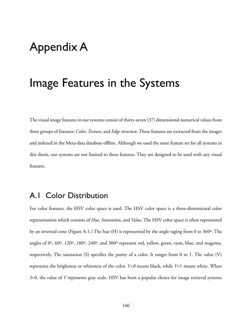
Appendix A
Image Features in the Systems
The visual image features in our systems consist of thirty-seven (37) dimensional numerical values from
three groups of features: Color, Texture, and Edge structure. These features are extracted from the images
and indexed in the Meta-data database offline. Although we used the same feature set for all systems in
this thesis, our systems are not limited to these features. They are designed to be used with any visual
features.
A.1 Color DistributionFor color features, the HSV color space is used. The HSV color space is a three-dimensional color
representation which consists of Hue, Saturation, and Value. The HSV color space is often represented
by an inverted cone (Figure A-1.) The hue (H) is represented by the angle raging from 0 to 360º. The
angles of 0º, 60º, 120º, 180º, 240º, and 300º represent red, yellow, green, cyan, blue, and magenta,
respectively. The saturation (S) specifies the purity of a color. It ranges from 0 to 1. The value (V)
represents the brightness or whiteness of the color. V=0 means black, while V=1 means white. When
S=0, the value of V represents gray scale. HSV has been a popular choice for image retrieval systems
106

including MPEG-7 standard [61][62][101][107] because this color representation is intuitive for
human perception [40][61].
Simple comparison in a color histogram [34][108] is sensitive to small color variations caused by
lighting conditions [104]. Instead, we use the color distributions in the HSV space proposed by
Stricker and Orengo [105]. In this method, the first three moments (the mean, the standard deviation,
and the third moment) from each of HSV channels are extracted [105]. Suppose is the value of i-
th color channel at the j-th pixel of an image, the three features are:
(1-1)
(1-2)
(1-3)
V (Value)
S (Saturation)
Red (0º)Cyan
YellowGreen (120º)
Blue (240º) Magenta
Black (V=0)
White (V=1)
H (Hue)
Figure A-1. The HSV color space.
pij
Ei1N---- pijj 1=
N∑=
σi1N---- pij Ei–( )2
j 1=
N∑⎝ ⎠
⎛ ⎞1 2/
=
si1N---- pij Ei–( )3
j 1=
N∑⎝ ⎠
⎛ ⎞1 3/
=
107

They are calculated for each of H, S and V. Therefore, the total number of color features is
for each image. Compared with color histogram comparison, the color moments are more robust
against small color variations [105].
A.2 TextureFor texture, we used Wavelet-based Texture Features [97][98]. First, each image is applied into Wavelet
Filter Bank [103] where the images are decomposed into 10 de-correlated subbands (3 levels) as shown
in Figure A-2. The upper left image in the wavelets image is the low frequency subband, and the lower
right image is the high frequency subband. For each subband, the standard deviation of the wavelet
coefficients is extracted. Therefore, the total number of this feature is 10.
A.3 Edge StructuresFor the edge structures, we apply the Water-Filling Algorithm [120] on the edge maps of the images.
We first pass the original images through the Sobel filter followed by thinning operation [36] to
generate their corresponding edge maps. From the edge map, eighteen (18) elements are extracted from
3 3× 9=
WaveletFIlterBank
fof1
f2
f3f4
f5f6f7
f8f9
Wavelet Image Feature Extraction
Figure A-2. The wavelet texture features
108

the edge maps. These features include the longest edge length, the histogram of the edge length, and
the number of forks on the edges.
109

Appendix B
Implementation Details of ImageGrouper and Query Engine
The source codes of ImageGrouper (Chapter 3,) the Query Engine (Chapter 4) and the traditional GUI
of image retrieval systems will be published under the Illinois Open Source License. In this section, the
implementation details of ImageGrouper and the Query Engine are explained. In addition, a brief
instruction for building the systems is given.
B.1 ImageGrouper
B.1.1 Structure of ImageGrouper User Interface
The current version of ImageGrouper is implemented in Java2 with Swing API. The user interface has
a layered structure (Figure B-1.) that consists of the following five components:
• Main Panel (MainPanel.java)
The base panel where the other panels are placed on. During the instantiation, the Main Panel
creates the other panels and places them on itself (Figure B-1.) Therefore, this panel is not visible
110
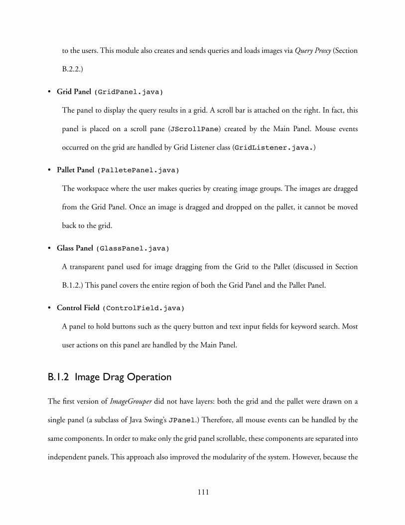
to the users. This module also creates and sends queries and loads images via Query Proxy (Section
B.2.2.)
• Grid Panel (GridPanel.java)
The panel to display the query results in a grid. A scroll bar is attached on the right. In fact, this
panel is placed on a scroll pane (JScrollPane) created by the Main Panel. Mouse events
occurred on the grid are handled by Grid Listener class (GridListener.java.)
• Pallet Panel (PalletePanel.java)
The workspace where the user makes queries by creating image groups. The images are dragged
from the Grid Panel. Once an image is dragged and dropped on the pallet, it cannot be moved
back to the grid.
• Glass Panel (GlassPanel.java)
A transparent panel used for image dragging from the Grid to the Pallet (discussed in Section
B.1.2.) This panel covers the entire region of both the Grid Panel and the Pallet Panel.
• Control Field (ControlField.java)
A panel to hold buttons such as the query button and text input fields for keyword search. Most
user actions on this panel are handled by the Main Panel.
B.1.2 Image Drag Operation
The first version of ImageGrouper did not have layers: both the grid and the pallet were drawn on a
single panel (a subclass of Java Swing’s JPanel.) Therefore, all mouse events can be handled by the
same components. In order to make only the grid panel scrollable, these components are separated into
independent panels. This approach also improved the modularity of the system. However, because the
111

grid and the pallet are independent components, the mouse events have to be handled separately. This
made image dragging handling complicated because the mouse events are sent different components
depending on the location of the mouse cursor. Moreover, since each panel has different coordinate
system (the upper left corner as the origin) the coordinates of the image has to be recalculated when
the image moves from one panel to the other. Furthermore, the amount of scroll on the grid has to be
considered.
In order to eliminate the overhead of mouse drag operations, a transparent panel
(GlassPanel.java) is introduced. This transparent panel is used for a temporal workspace for
mouse dragging operations. When the system starts, the Glass Panel is inactive and does not receive
any events. When the user starts dragging an image on the Grid Panel, the system activates Glass Panel
and transfers the images to the same location on the panel (Figure B-2 (1).) While the user is dragging
the image, it is painted on the glass (Figure B-2 (2).) When the user releases the mouse button over the
pallet, the image is dropped on the Pallet Panel (Figure B-2 (3).) If the image is still over the grid, it is
returned to the original location the grid. Once the image is dropped on the pallet, it cannot be moved
back to the grid. Now it is drawn on the Pallet Panel even if it is dragged. When the images are moved
Palet tePanelGridPanel
MainPanel
ControlPane
GlassPanel
ane
Figure B-1. Layered structure of ImageGrouper user interface
112

between the panels, the mouse location in the origin is translated for the coordinate system of the new
panel. This approach realizes much smoother image dragging operation because the mouse coordinates
need to be translated only at the beginning and the end of the drag operations.
B.2 Query Engine
B.2.1 Overview of the Query Engine
In this section, we explain the implementation of the Query Engine. The Query Engine receives a
query from a user interface and then returns the result. The query results include a list of relevant
images and their auxiliary information such as filenames. Our engine is versatile in that the same engine
can handle requests from different user interfaces including ImageGrouper and 3DMARS. The system
dynamically selects a search algorithm and a result format based on the request types. For example,
when the engine receives a query from 3DMARS, it returns the 3D locations of the result images as
well. Meanwhile, the engine need to process group information when communicating with
ImageGrouper. The system will be published with an open source license.
Palet tePanelGridPanel
ControlPa(1)
(3)
lPa
GlassPanel(2)
Figure B-2. Image Dragging from the Grid to the Palette.
113

The current system is implemented in C++ for the maximum computation speed. Query algorithms
like Group Biased Discriminant Analysis (Section 4.3) involve lots of vector and matrix calculations. In
order to improve the speed of the system, we used a linear algebra package called CLAPACK [2]. This
library is commonly used for scientific computation. CLAPACK and its Fortran version LAPACK
(Linear Algebra PACKage) separate the basic vector / matrix computation as Basic Linear Algebra
Subprograms (BLAS) so that the system can take advantages of vector processing units of different
CPUs or shared memory parallel processors. Various implementations of BLAS (or its C version
CBLAS) have been developed. We chose an implementation known as Automatically Tuned Linear
Algebra Software (ATLAS) [4]. ATLAS is a very popular open source implementation of CBLAS that
is used by many commercial systems. For SPARC Solaris machines, we used Sun Performance Library
[106].
Because LAPACK and BLAS were originally designed for Fortran77, the functions in CLAPACK and
CBLAS have cryptic names and require many arguments. In order to make coding of the Query Engine
easier, we provided wrapper functions in a separate source file (matfunc.cc) and a header file
(mathfunc.h) so that the user can easily compile the system with another linear algebra packages
such as Intel Math Kernel Library [45]. The functions included in this source file ranges from simple
vector and matrix calculations to higher-level functions such as covariance matrix and generalized
eigenvectors. Our matfunc functions are very simple and generic. Therefore, it makes easier for the
user to implement other algorithms. The detail of the search algorithms used in our Query Engine is
described in Chapter 4.
114

B.2.2 System Configurations
The Query Engine and the User Interfaces can run in two configurations. The first configuration is
Client-Server configuration where the Query Engine (server) and the user interface (client) are located
on different machines and communicate with each other over networks. The second configuration is
Standalone configuration where the Query Engine and the User Interface reside in the same machine.
The same Query Engine can be used for both configurations. The main component of the engine is
stored in a shared library (or DLL for Windows) named libgroup.so (for UNIX.) They are named
libgroup.dylib for Mac OS X, and group.dll for Windows. No recompilation is required to
switch between two configurations.
The client and the server do not communicate directly. Instead, the client dynamically loads a proxy
component (Query Engine) to connect with the engine. Different proxies connect a client with a server
in different ways. Every proxy, however, has a common interface to the clients (defined in
QuerySender.java,) so that the clients can communicate with any servers in the same manner.
B.2.3 Client-Server Configuration
Figure B-3 shows the overview of the Client-Server configuration. In this configuration, the Query
Engine server and the user interface client communicate via HTTP [29] over TCP/IP. The server is
implemented as a Java Servet that works with Apache Web Server. When the Servlet starts, it loads the
body of the Query Engine stored in libgroup.so. The engine then loads the metadata and waits for
query requests. The Servlet parses HTTP request from a client and passes it to the engine. The Servlet
part of the system is written in Java (GroupImageServlet.java) and the main engine component
115

is written in C++. They are connected by Java Native Interface (JNI) as defined in
GroupImageServlet.h and GroupImageServletImp.cc.
Since the server is implemented as a Servlet, the user can send a query from a web browser by typing
the address of the servlet with the query parameters such as:
http://chopin.ifp.uiuc.edu:8080/servlets/GroupImageServlet?Type=Que-ry&Id=3436&Rel=1.0&Id=3478&Param=15
In this example, the user is requesting 15 similar images that are similar to an image with ID=3436.
Then, the user sees the result as a list of image IDs.
On the client side, the User Interface sends query to the server via a query proxy. This proxy translates
a query request from a client into a HTTP message and sends it to the server. Then, the proxy receives
the result from the server and passes it to the client. The query proxy is implemented in Java (in
RemoteQuerySender.java, a subclass of QuerySender) for ImageGrouper and the traditional
user interface (Chapter 3), and in C++ for 3DMARS (Chapter 2).
One advantage of this configuration is that multiple user interface clients can communicate with a
single engine simultaneously.
User Interface Query Engine
Servlet
Web Server
Network (HTTP, TCP/IP)
Client Server
JNI
Query Proxy (RemoteQuerySender)
Figure B-3. Client-Server configuration.
116

B.2.3.1 Standalone Configuration
Figure B-4 shows the structure of the Standalone configuration. The user interface and the Query
Engine reside in the same machine. This configuration has a three-layer structure. When the user
interface starts, it loads a query proxy named LocalQuerySender. Then, it loads the shared library
libgroup.so and initializes a query engine. The proxy is implemented in Java
(LocalQuerySender.java.) It communicates with the Query Engine via Java Native Interface.
Because there is no network overhead, this configuration has a faster query response than the client-
server configuration.
B.3 Building Instructions
B.3.1 Directory Structure
The directory structure of the main system package is as follows:
lib/access/lib/shared/server/
User Interface
Query Engine
JNI
Query Proxy (LocalQuerySender)
Figure B-4. Standalone configuration with a local query engine
117

grouper/tradgui/
Each directory contains the source codes and the makefiles. The Query Engine is stored in server
directory. ImageGrouper and the traditional GUI are stored in grouper and tradgui, respectively.
The query proxy for the standalone configuration (LocalQuerySender.class) is automatically
copied into classes subdirectories in tradgui and grouper.
lib directory stores libraries which are shared by all components. The data formats exchanged between
the client and server are defined in shared subdirectory. The template of the query proxy (Section
B.2.2) is also defined here. They are required to compile the other components. The query proxy for
client-server communication is defined in access subdirectory. When these libraries are compiled
and installed, the makefiles copy archived libraries (shared.jar and ServletAccess.jar) into
grouper and tradgui directories.
B.3.2 Building Systems
Included makefiles support Solaris (with Sun Performance Library), Mac OS X, and Windows
(Cygwin) at the time of writing. The users of above systems should be able to compile the system
without any problems. For other systems, the user may need to edit makefiles slightly.
B.3.2.1 Additional Libraries
In order to build the systems, the user needs to obtain linear algebra packages such as CLAPACK and
CBLAS as discussed in Section B.2.1. They are not part of the main distribution of the system. While
the users can easily compile those libraries by themselves, compiled binaries are available from the
author by request for Solaris, Mac OS X, and Cygwin. Compiled binaries of ATLAS for various
118

platforms including Linux and AIX are also available from ATLAS’s official web site at http://
math-atlas.sourceforge.net/.
For Cygwin systems, the user also needs a Java wrapper, which is included in
cbir_support_cygwin subpackage. For more detail, see README_Cygwin.txt in the main
directory of the main distribution.
B.3.2.2 Setting Java Parameter
Because lib, grouper, and tradgui are Java2 programs, they can be compiled with the same
common makefile for all platforms. The location of Java SDK, however, varies from systems to systems.
Therefore, the users need to set an environment variable to match the configuration of their own
systems. For example, if Java is installed in /usr/local/bin, set JAVAC environment variable from
a console as follows:
% setenv JAVAC /usr/local/bin/javac
Or the user can set the variable in the makefile of the main directory.
B.3.2.3 Modifying Server Makefile
The source codes in server subdirectory are written in standard C++ and Java. The main makefile
automatically chooses a suitable platform-specific makefile based on OSTYPE environment variable.
Currently, makefiles for OSTYPE = solaris (Solaris), darwin (Mac OS X) and cygwin
(Windows) are included. The users may need to modify some variables in these makefiles so that the
locations of linear algebra packages match their environment. Especially, LIBDIR specifies the location
of CLAPACK libraries, and ATLAS_TOP specifies the location of ATLAS.
119
B.3.2.4 Compiling
To compile all components, simply type:
% gmake all
In order to compile a specific component, for example to compile only lib directory, type:
% gmake lib
B.3.3 Running Systems
To run ImageGrouper and the traditional GUI, the user has to change parameters in html files especially
for the image file location and the meta file location.
B.3.3.1 Image File Location
For example, to run systems with images stored in /workspace/video_databases/corel/t1/
jpg, parameter “imagebase” needs to be changed to:
<PARAM NAME = imagebase VALUE = "file:///workspace/video_databases/corel/t1/jpg">
When the user uses an image database on a web server, it can be changed to, for example:
<PARAM NAME = imagebase VALUE = "http://myserver.com:8080/grouper/class-es/corel/jpg">
B.3.3.2 Metadata File Location
To run the system on a PC locally, the metadata files have to be copied into the local hard disk and
“metapath” parameter has to be set to the file location such as:
<PARAM NAME = metapath VALUE = "/Users/myaccount/corel/">
B.3.3.3 Server URL
For client-server configuration, the URL of the server (Java Servlet) has to be specified as well. For
example:
120

<PARAM NAME = servlet VALUE = "http://chopin.ifp.uiuc.edu:8080/servlets/GroupImageServlet">
B.3.3.4 Starting Systems
Small shell scripts (or batch files) are provided to run ImageGrouper and the traditional GUI. To run a
system on UNIX terminal, the user types:
% ./runclient.sh (for remote client)
or
% ./runlocal.sh (for local standalone client)
In Microsoft Windows,
> RUNCLIENT.BAT (for remote client)
or
> RUNLOCAL.BAT (for standalone)
In order to run the systems as a standalone system, the server has to be compiled too.
121

122
Vita
Munehiro Nakazato was born in Tokyo, Japan on June 5, 1971. He graduated from Keio University in
1995 with a degree of Electrical Engineering. He also received a master degree in Computer Science
from Keio University in 1997.
Recommended