1 3 9(
V393.R46

'- ) 'r
J.p
*'~~ ' ' W
L, t L
,%
.1
1,.4
*rir
tv
r 'L 1' 4
p~~. -1tA'
200 .- IJ ? ;F7
It '-41t '' 3
4W -T.
TuIL-~~~~~~~~ i&4,r~ *y~ A" F' '

THE FRICTIONAL RESISTANCE AND TURBULENT BOUNDARYLAYER OF ROUSH SURFACES
by
Paul S. Granville
Report 1024
-- INN
June 1958

TABLE OF CONTENTS
Page
A B ST R A C T ......................................................................................................................... 1
INTRODUCTION ..................................................................................................................... 1
BOUNDARY-LAYER CHARACTERISTICS FROMSIM ILA R IT Y LA W S .......................................................................................................... 3
G eneral ........................................................................................................................... 3
Inner Law or Law of the Wall ....................................................................................... 3
Outer Law or Velocity-Defect Law ........................................................................ 4
Logarithm ic V elocity Law ................................................. .......................................... 4
Types of Flow Regimes on Rough Surfaces ........................................................... 6
Sublayers within Turbulent Shear Flows ..................................................................... 7
Velocity Law for the Laminar Sublayer ................................................................. 9
Velocity Law for the Transitional Sublayer of Smooth Surfaces ............................. 9
Velocity Law for the Transitional Sublayer of the General Rough Regime .......... 13
Velocity Law for the Transitional Sublayer of the Fully Rough Regime ............. 14
Boundary-Layer Parameters ........................................................................................ 17
FRICTIOYAL RESISTANCE OF FLAT PLATES .................................... .......... 20
G eneral ............................................................................................................................ 20
F ully Rough R egim e ............................................. .................................................. 24
Q uasi-Smooth R egim e ................................................................................................... 25
Engineering Roughness .................................................................. 26
APPLICATION OF THE GENERAL LOGARITHMIC RESISTANCEFORMULA TO ARBITRARY ROUGHNESS ................................................................... 28
Preparation of Resistance Diagrams from Resistance Characterizations ............. 28
Resistance Characterizations from Plate Tests .................................... ......... 30
Prediction of Full-Scale Resistance from Plate Tests ......................................... 33
LOCAL SKIN FRICTION COEFFICIENTS AND SHAPE PARAMETERS ................ 35
G eneral ............................................................................................................................ 35
F ully R ough R egim e ..................................................................................................... 36
Quasi-Smooth R egim e ................................................................................................... 37
E ngineering R oughness ................................................................................................ 38
Preparation of Local Skin Friction Coefficient and Shape ParameterDiagrams from Resistance Characterizations .................................... .......... 39
Preparation of Local Skin Friction Coefficient and Shape ParameterDiagrams from Plate Tests ...................................... .................... ........ ....................... 40
i*tc"dy l 1 131 -- ill I II
Page
NUMER IC AL RESULT S .................................................................................................... 41
ACKNO WLE DGMENT ........................................................................................................ 44
R EF EREN CE S ............................. .............................................................................. 44
LIST OF ILLUSTRATIONS
Figure 1 - Resistance Characterization for Roughness in Pipes............................ 7
Figure 2 - Sublayers within Turbulent Shear Flows ....................... ......... ....... 8
Figure 3 - Comparison of Various Formulations for Transitional Sublayer of
Smooth Pipes ......................................................... ...................................... 12
Figure 4 - Variation of Transitional Sublayer Factors for Nikuradse SandR ough P ipes .................................................................................................... 14
Figure 5 - Plot of Inner Law for Nikuradse's Sand Rough Pipe Data ................. 16
Figure 6 - Plot of Inner Law for Nikuradse's Sand Rough Pipe Data ..................... 16
Figure 7 - Resistance Diagram for Rough Plates with Sand Roughness and
Engineering Roughness ............................................................................. 31
Figure 8 - Resistance Characterization of Roughness from Flat PlateResistance Data .......................... ..................................... 32
Figure 9 - Resistance Prediction Diagram for Pough Plates ...................................... 34
Figure 10- Values of B2 for Sand Roughness in Pipes and on Flat Plates ............ 42
Figure 11- Coefficients of Total Resistance for the Fully Rough Regime ............. 43
Figure 12 - Local Skih Friction and Shape Parameter for the Fully Rough
Regime of Flat Plates ................................................................................. 43
LIST OF TABLES
Table 1 - Summary of Factors for the Velocity Laws of TransitionalSubla yers .......................................................................................................... 1 7
Table 2 - Velocity Profile Integrals ............................................................................. 18
Table 3 - Numerical Values of Factors ......................................................................... 41
I 1.1

NOTATION
a1 , a2'
B 1, B2 ,
a3 , a4
B3
Bl s
B2, R
B,2
Cf
CT
Cl, C2 C3' C4
D 2
e
F
G
H
11, '2
J1, "J2
k, kl, k 2, . ..
k*
*k
L
1
M1 , M2
m
Slope of logarithmic velocity law
Linearization constants
Intercepts of logarithmic velocity law; see Equations[7], [8], and [10]
B1 for smooth surfaces
B2 for fully rough regime
Derivative of B2 with respect to In k*, Eouation [76]
Derivative of B2 with respect to In k*, Equation [77]
Coefficient of total resistance; see Equation [67]
Coefficient of local resistance; see Equation [13]
Linearization constants; see Equations [91] and [95]
Velocity profile constants; see Table 2
Base of natural logarithms
Outer law function, Equation [4]
Inner law functions, Equations [2] and [3]
Subscript for quantities at junction of inner and outerturbulent sublayers; see Table 2
Shape parameter, Equation [631
Integrals of outer law velocity profiles; see Table 2
Transitional sublayer factors, Equations [42] and [441
Linear parameters defining rougnness
Roughness Reynolds number; see Equation [2]
Value of k* at start of fully rough regime, Equation [53]
Value of k* at end of quasi-smooth regime
Subscript for quantities at junction of laminar and tran-sitional sublayers; see Table 2
Mixing length
Constants in logarithmic resistance formulas for flatplates, Equations [93] and [98]
Constant in logarithmic resistance formula for flat plateswith engineering roughness, Equation [117]
~ I I I -I II I II -- _----- ,- -----~--~1-~1--~1~1

N1, N1, N2 Constants in logarithmic resistance formulas for flatplates, Equations [94], [99] and [103]
01, 02 Constants in local resistance formulas, Equations [145]and [150]
P, P', P2 Constants in local resistance formulas, Equations [1461,[156] and [151]
Rf Frictional resistance
Rx Reynolds number based on length
R 0 Reynolds number based on momentum thickness, Equation[61]
r Factor given in Equation [1721
s Subscript representing smooth conditions
T Subscript for quantities at junction of transitional andinner turbulent sublayers; see Table 2
U Velocity at outer edge of boundary layer
u Tangential velocity in boundary layer
u' Fluctuation in u
uT Shear velocity
v' Fluctuation in normal velocity
x Distance along boundary layer
z* Nondimensional x, Equation [124]
y Normal distance from wall
y* Nondimensional y
al, a 2 Velocity profile constants; see Table 2
f 1, 02 Velocity profile constants; see Table 2
y Constant in logarithmic resistance formula for flat plateswith engineering roughness, Equation [1161
SBoundary layer thickness
8* Displacement thickness
C Boussinesq eddy viscosity, Equation [221
0 Momentum thickness
K Slope of e with respect to y
x Constant for engineering roughness, Equation [1091
U II

CI Viscosity of fluid
v Kinematic viscosity, p/p
p Density of fluid
a Local resistance parameter, U/u.,
" Shearing stress
T" Shearing stress at wall
- - RI1 - gl l ill I go 11 -- Z

ABSTRACT
By means of the similarity laws of the turbulent flow in boundary
layers, a general relation is developed for the frictional resistance of
flat plates with arbitrary roughness from which logarithmic formulas are
obtained for the special cases of the fully rough regine, the quasi-
smooth regime, and engineering roughness. Among other uses, this
general relation permits for the first time a simple rational extrapolation
to full-scale conditions of the frictional resistance of model plates
covered uniformly with any irregular full-scale roughness encountered
in practice. Furthermore, for calculations of turbulent boundary layers
in pressure gradients on rough surfaces, relations are derived for the
local skin friction and velocity profile shape parameter in terms of mo-
mentum thickness Reynolds number. Simplified relations are also de-
rived for the velocity profile of the transitional sublayer in the vicinity
of a rough surface.
INTRODUCTION
The analysis and prediction of the frictional resistance or drag of rough surfaces pre-
sents in general a more complex problem than that of smooth surfaces owing to the geometric
diversity of roughness and the accompanying involved effect on turbulent flow.
Since research into the fundamentals of turbulence has yet to achieve a method for pre-
dicting frictional resistance, recourse as in the case of smooth surfaces is made to the sim-
ilarity characteristics of the mean-velocity profiles of shear flows for a general method of
analyzing the resistance of rough surfaces.
For turbulent shear flows, such as fully developed viscous flow in pipes or boundary-
layer flow on flat plates, the two laws which provide similarity in the mean-velocity profile
by linking it to the wall shearing stress are:
1. The inner law or law of the wall which applies to the flow immediately adjacent to the
solid boundary.
2. The outer Law or velocity-defect law which applies to the remaining outer region of the
shear flow.
The overlapping of the range of application of the two laws requires a logarithmic functional
form for both similarity laws within the common region of overlap.
The similarity laws of the velocity profile were originally developed for pipe flows by
Prandtl I and separately by Von Karman,2, 3 though with some significant differences. Prandtl
1References are listed on page 44.
000 141wi WIMIN

used the logarithmic form for the velocity profile of the whole flow which in effect assumed
the region of overlap of the two similarity laws to extend over the whole flow. Von Karman,on the other hand in a more general presentation, used the logarithmic form for only a limited
region of overlap and wrote the outer law as an unspecified functional relation for the flowoutside the region of overlap. The difference between the Prandtl and Von Karman proceduresis not significant for pipe flows since a logarithmic form fits very closely most of the flow,but it is significant for boundary-layer flows on flat plates since a logarithmic form fits ade-quately only about 15 percent of the flow.
Inasmuch as the differences between pipe and flat-plate flows were not apparent at thetime, Prandtl and Schlichting 4 used the simpler Prandtl procedure of a logarithmic form forthe whole boundary-layer flow as well as numerical values from pipe tests in determining theresistance of rough plates from Nikuradse's s tests on pipes coated with sand grains. Conse-quently, one of the purposes of this report is to determine the resistance of sand-coated platesby applying Von Karmn's procedure of a limited logarithmic region together with the some-what different numerical values from flat-plate tests.
More importantly, the whole subject of the application of the similarity laws to the re-sistance of rough plates is developed in detail. The logarithmic form of the similarity lawsin the region of overlap is derived in a simple fashion which emphasizes the nature of the re-sulting constants. Detailed consideration is given to delineating the different sublayerswithin the boundary layer. Expressions are derived for the velocity profile of transitionalsublayers of rough surfaces by an extension of a method of Squire 6 for smooth surfaces. Theboundary-layer factors of displacement thickness, momentum thickness, and shape parameterare determined for rough surfaces by combining integrated quantities of the velocity profilesof the separate sublayers.
The relation for momentum thickness is then used to determine the coefficient of totalresistance of flat plates as a function of Reynolds number and relative roughness in terms ofa local-resistance parameter for the general case of roughness. Then by eliminating the local-resistance parameter and dropping terms which become negligible at larger boundary-layerthicknesses, a simpler logarithmic formula is obtained for the total resistance coefficient offlat plates with arbitrary roughness. From this, special logarithmic resistance formulas aredeveloped for the special cases of the fully rough regime, the quasi-smooth regime, and engi-neering roughness.
The general logarithmic resistance formula is used to prepare resistance charts fromempirical roughness characterizations, to obtain roughness characterizations from total re-sistance data, and to predict full-scale resistance from plate tests with arbitrary roughness.The last procedure should be especially useful in studying the frictional resistance of shiphulls in newly painted and in fouled conditions. Towing a representative sample of the hullroughness would be required instead of difficult full-scale trials.
I ---~---~r I --rr ---~-- I II-

Finally relations are derived for the local skin friction and the velocity profile shape
parameter for use in calculations of turbulent boundary layers in pressure gradients. A meth-
od of obtaining such information from towing tests of plates with arbitrary roughness is also
included.
BOUNDARY-LAYER CHARACTERISTICS FROM SIMILARITY LAWS
GENERAL
First, an important distinction should be emphasized between the similarity laws and
their historical association with turbulence hypotheses, like the mixing-length theory, which
have become somewhat untenable by reason of more detailed experimental investigations 7 ' 8
into the nature of energy transfer in shear flow. As statements of general functional relation-
ships, the similarity laws can have their basis in purely dimensional arguments supported by
experimental data and thus be made independent of the mixing-length and like theories.
In the past it was mainly for the purpose of deriving specific functional relations that
hypotheses concerning the turbulence mechanism had been introduced into the analysis.
These were the mixing-length theory and assumptions about the laminar sublayer by Prandtl 1
in obtaining the logarithmic form of the inner law, and a similarity hypothesis of the turbulent
flow pattern by Von Karman 3 in formulating his particular expression for the outer law. All
this can be avoided since the logarithmic form can be derived from the overlapping of the inner
and outer laws and the outer law elsewhere can be analytically treated as an unspecified func-
tion in arriving at the desired resistance formulas.
INNER LAW OR LAW OF THE WALL
Close to the wall or solid boundary the distribution of the mean velocity u of the tur-
bulent flow parallel to the wall is considered to depend on the normal distance y away from
the wall, the shearing stress 7 at the wall, the density p and viscosity /i of the fluid, and
various linear parameters defining the roughness of the wall k, k l , k2, . . . , or
u = f(y, r, , p, I, k, kl, k2,...) [1]
There is in addition the boundary condition at the wall, u = 0 at y = 0, to be satisfied. By di-
mensional analysis the variables can be grouped significantly into the following nondimen-
sional ratios:
U = f y*, k*, , , .. . [2]
or
U kkSf2 k*, -,- . . . [3]
U k k I, k 2
_I I

where u.= V--- is a factor having the dimensions of velocity and hence called the friction
UTY ukor shear velocity, v - is the kinematic viscosity of the fluid, y* = -, and k* =
P v
Empirically, Equation [2] or [3] which is the statement of the inner law is uniquely defined for
fully developed turbulent flow in pipes regardless of the pipe diameter Reynolds number. Asimilar but somewhat different numerical relationship holds uniquely for flat plates independ-
ent of plate length Reynolds number. In addition the inner law has been found to be independ-
ent of pressure gradients. 9
OUTER LAW OR VELOCITY-DEFECT LAW
For the turbulent stream at some distance away from the wall the velocity-defect ratio
U-u-, where U is the maximum velocity, is found experimentally to be directly independent ofu 7
viscosity and a function only of its relative position in the flow or
U-u y- F [4]
where 8 is the thickness of the shear flow. The boundary condition u = U at y = 8 is to bealso satisfied. The function F has been found empirically to be independent of Reynolds
number and, most significantly, of the roughness of the wall. 3
The function F is numerically different for boundary-layers on flat plates than for pipeflow owing mainly to the presence of the free outer boundary of boundary-layer flow which hasbeen found to have undulating characteristics. 9 It is also markedly affected by longitudinal
pressure gradients. 10
LOGARITHMIC VELOCITY LAW
Within the boundary layer there is a region where both the inner and outer laws are con-
sidered valid. This overlapping leads to a logarithmic relation which will now be derived by
a simplified version of Millikan's 1 1 original demonstration.
Equating the derivative of velocity u with respect to distance y of the inner and outer
laws, Equations [2] and [4], results in
du Ur af u, dF=- - [5]
ay v ay* 8 d(y/8)
or
r~ IIIII 1 ~s I I I II I -- c IC I I -----

af /\ dFy* - = - A [6]
ay* \ d(y/8)
Since the left-hand side of Equation [6] is only a function of y* and roughness parametersk k
k*, --, . . . and the right-hand side is only a function of-, the only quantity satisfying
these conditions is a constant A independent of all these variables.
From the left-hand side there results after integration
f 1 A In y* + B 1 k*, , , ... [7]U, k1 k2
k kwhere the constant of integration B 1 is necessarily a function of k*, -,-, ... from the in-
kI k 2
tegration of a partial derivative. Equation [7] is the statement of the inner law in the region
of overlap. An alternate expression is
-Aln - + B 2 k*, -,n' [8]u k 'k 1 k 2
where
B 2 = B 1 + Aln k* [9]
Fromthe right-hand side of Equation [6] the outer law in the region of overlap is
U-u yF = - . In - + B3 [10]Ur a
This establishes the logarithmic form of both the inner and outer laws in the region of
overlap. A very important result is that the factor B 1 or B 2 is seen to be solely a function
k kof roughness Reynolds number k* for a particular roughness configuration,-, -, . . . ,
k1 k2
and that A is independent of roughness. Hence the frictional effects of any particular rough-
ness may be considered defined when B 1 or B2 is experimentally determined as a function
of k*. This will be termed the resistance characterization of a roughness configuration.
Now equating the velocities from the inner and outer laws in the region of overlap
gives important relations for the local skin friction.
m mIY il 11N6Al I.I Wli=V

From Equations [7] and [101
U ut8a -=Aln -+B + B 1 [11]
Ur v
or from Equations [81 and [10]
U 8a -- = Aln - + B3 + B 2 [12]
UT k
where a is a local resistance parameter. With local coefficient of resistance
27. UT 2 2C - 2 - = - the preceding equations appear as
pU2 U 2
- = A n + B, + B, [13]
or
Aln - + B3 + B2 [14]=C k
TYPES OF FLOW REGIMES ON ROUGH SURFACES
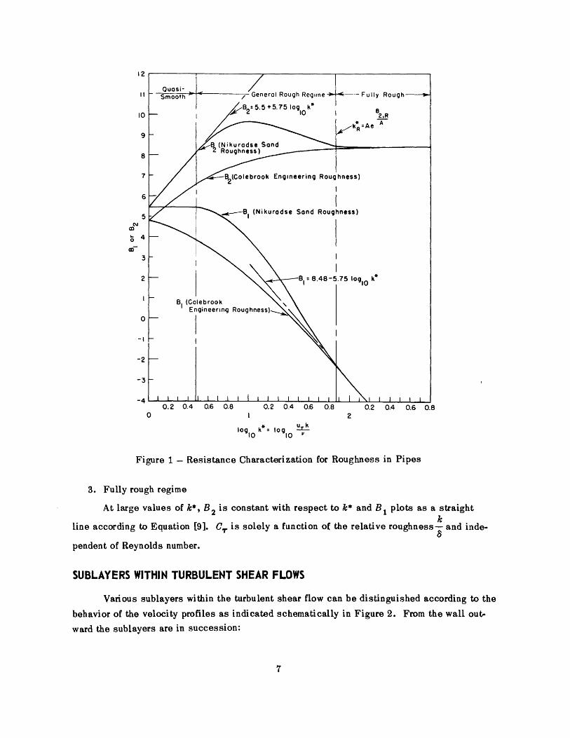
In Figure 1, which shows the resistance characterization for Nikuradse's sand rough
pipes, it is seen that B 1 is constant for small values of k* and that B 2 is constant for large
values of k*. For intermediate values of k*, both B 1 and B 2 vary with k*. From this the fol-
lowing classification of turbulent flow past rough surfaces can be made which is significant
from the viewpoint of skin friction:
1. Quasi-smooth regime
For small values of k* starting from zero, B 1 is constant with respect to k* and has
the same value as for a smooth flow. According to Equation [91, B2 then plots as a straight
line. Most iniportant of all as given by Equation [13] the local coefficient of resistance C,.US
is the same as for a smooth surface and is solely a function of Reynolds number -.
2. General rough regimeUS
With B 1 and B 2 both varying with k*,,C . is a function of Reynolds number- and
relative roughness .
~~ 1 111 ---- I I __ Z 3 -- ~---
Quasi- /II Smooth / General Rough Regime ---- Fully Rough
/10B2= 5.5 +5.75 ogo10 k 2,R
kR Ae A
I(Nikurodse Sond8 Roughness)
7 B (Colebrook Engineering Roughness)
6
5 B1 (Nikurodse Sand Roughness)
2- Bi = 8.48-5.75 logo10 k*-
2
-3
-40.2 0.4 0.6 0.8 0.2 0.4 0.6 0.8 0.2 0.4 0.6 0.8
0 I2
log k* log10 IlO 1
Figure 1 - Resistance Characterization for Roughness in Pipes
3. Fully rough regime
At large values of k*, B 2 is constant with respect to k* and B 1 plots as a straight
line according to Equation [9]. Cr is solely a function of the relative roughness- and inde-
pendent of Reynolds number.
SUBLAYERS WITHIN TURBULENT SHEAR FLOWS
Various sublayers within the turbulent shear flow can be distinguished according to the
behavior of the velocity profiles as indicated schematically in Figure 2. From the wall out-
ward the sublayers are in succession:

Outer Turbulent Sublayer 3_
Inner Turbulent Subloyer Wo
Laominor Trans tional SublayerSublayer 7l--ll////l//l/ /i ,// / //
Solid Wall
Figure 2 - Sublayers within Turbulent Shear Flows
1. Laminar sublayer
This is the very thin layer in contact with the wall where the flow is laminar and con-
sequently the shearing stress 7 is given by
duS= du [151
dy
The thickness of the laminar sublayer diminishes with increasing roughness, and finally van-
ishes in the case of the fully rough flow regime.
2. Transitional sublayer
In this layer the effect of turbulence appears so that the shearing stress is given by
du7 = -y pu'v' [16,]
dy
where - p u'v' is the Reynolds turbulent shearing stress.
3. Inner turbulent sublayer
The inner and outer laws overlap in this layer resulting in the logarithmic velocity law.
4. Outer turbulent sublayer
In this region the wall has no direct effect and the velocity law is the nonlogarithmic
part of the outer law.
- .- b- - I---- -- --_011 01 .01 111 110, IN--~C

VELOCITY LAW FOR THE LAMINAR SUBLAYER
Inasmuch as the inner law Equation [2] provides only the general statement that theu
velocity ratio - is a function of Reynolds number y* (laminar flow is independent of rough-U T
ness), other considerations must be applied in order to obtain a specific functional relation-
ship for the laminar sublayer. If the laminar motion within the sublayer is assumed essen-
tially a parallel flow, the shearing stress r is given as
du [17]
dy
Within the thin sublayer the variation of r with y is negligible; hence
T = TW
Consequently
and with u = 0 at y = 0,
or
[181
du -r
dy ji
,rwU= - y
[19]
[201
[21]
Empirical verification for
in a closed channel.
this relation has been obtained by Laufer7 by measurements
VELOCITY LAW FOR THE TRANSITIONAL SUBLAYER OF SMOOTH SURFACES
Expressions for the velocity law of the transitional sublayer for smooth surfaces have
been derived by various authors on the basis of assumptions concerning the variation of the
turbulent shearing stress with y. In general, since the shearing stress has both laminar and
turbulent contributions,
duT = I- - pu [i']
dy
---- -- ~ ~~~11111111N1
[16]

where -p u'v' is the Reynolds stress formed by the average of the turbulent velocity fluctu-
ations u'and v'in the x and y directions respectively. If the Boussinesq eddy viscosity E
is introduced where
u'v"du
then
duS= p (v+ )dy
dy[23]
[22]
If it is assumed that the variation of r with y across
7 = and
duu =( +)dy
the thin sublayer is negligible, then
[24]
Various investigators have assumed in effect different variations of e with y.
Squire 6 by dimensional reasoning and by considering the turbulence effect to
just at the outer edge of the laminar sublayer uses a linear variation of e across the
tional sublayer or
f= K u .,(y-yL)
start
transi-
[251
where x is a constant of proportionality and YL is the thickness of the laminar sublayer.
Other authors use the mixing-length hypothesis wherein
[26]12 du
I dy
1 being the mixing length. Rotta 12 and Hudimoto1 3 independently assume
S= K2 (y-YL)
I dy
[27]
[28]
Hama 1 4 uses for both the laminar and transitional sublayers
i~arU ----~I I I~ 11~- "-L~- -U ~---~.~..- - ~--..- - I I -- -~s~- aC ^I----CILI ----r- s -

I = Ky 2
or
e= K2y 4 y [301dy
whereas Van Driest s5 assumes a still more complicated relation
=Ky l-e const
or
2const d[
=K2y 2 1-e const [32]/ dy I
The procedures of both Squire and Rotta lead to expressions in closed form, that of
Squire being much simpler. On the other hand Hama obtained a much more complicated expres-
sion involving elliptic integrals and Van Driest obtained a still more unwieldly expression re-
quiring numerical integration. In Figure 3 where the various formulations are compared with
Laufer's 16 pipe data, it is to be noted that the simple expression of Squire is an adequate
approximation. The method of Squire will be extended in this report to cover the case of
rough surfaces. However, full credit is due Rotta 1 2 for first analyzing the transitional sub-
layers of rough surfaces.
Squire's procedure for smooth surfaces will be now completed. Substituting Squire's
e, Equation [251, into Equation [241 results in
dy v + K1u(Y-YL)
Integrating and utilizing the initial condition that
U u-ryL- -- at y = YL [34]
UT V
[29]

2 3 4 5 6 789 2 3 4 5678910
0Y
2 3 4 5 6789103
Comparison of Various Formulations for TransitionalSublayer of Smooth Pipes
u 1 u(y- ) 1-In + - - -In
U7 K V K K
urYL
v
u
UT
where
AAln(y*-Bi + Aln A) + B1
1A=
K
B = YL* - Aln A
YL *= B + AlnA
24-
22
20
18
uu 12
Figure 3 -
yields
[35]
[361
[371
[38]
[391
*C-U*~IIII -III I I 1 13 '- 'II ---------~----------r ~_I_~LnP'

INNN11 " , 61 1WI W1
For large y* the velocity law asymptotically becomes
U- A lny* + B 1 [40]
UT
which is the form for the logarithmic law. Hence the A and B 1 of Equation [40] and those of
the inner law Equation [7] are identical.
It is to be noted that Equation [39] gives the thickness of the laminar sublayer when
values for B 1 and A are substituted in the expression.
VELOCITY LAW FOR THE TRANSITIONAL SUBLAYEROF THE GENERAL ROUGH REGIME
The velocity law for the smooth transitional sublayer, Equation [36], can be written as
U- A In (y*-J) + B [41]
uT
where
eJ1 = B-Aln A= yL *-A [42]
A
Since B1 is a function of k* for a particular roughness, then J1 and YL* are also functions
of k*. For the general rough regime J1 will have a limiting value of -A since YL * is zero
for the case of the fully rough regime.
The velocity law for the transitional sublayer of the general rough regime may be re-
stated as
-u =A -J + B2 [43]
where
y, *-A J (y)L AJ 2 = = [44]
k* k* k*
Also
AB +Aln-
S[45]

7
6
5
4
JJ0 I
-3
-I -
-2
Regime-5 --2
2 3 4 56789 2 3 4 56789 2 3 4 5 6 7893I 10 k 102 10
Figure 4 - Variation of Transitional Sublayer Factorsfor Nikuradse Sand Pough Pipes
Figure 4 shows a plot of YL*, J1,, a n d J 2 as a function of k* calculated for Nikuradse's sandrough pipes.
VELOCITY LAW FOR THE TRANSITIONAL SUBLAYER OF THEFULLY ROUGH REGIME
In this case the laminar sublayer has vanished, YL = 0, and the plane of reference fory, y = 0, is defined where the velocity u is zero on an average over the rough surface. Thereis then an initial shearing stress due to turbulence represented by to at the start of the tran-sitional sublayer. Then
f = 0 + K UY [46]
and
du u2
[47]dy v+eo +K u r y
~D~n*p.~~4~mCI ~ C --

Integrating and utilizing the initial condition u = 0 at y = 0 results in
U 1 K UTy
U K V+
= An -J 2 + B2UT
where
B 2
J2 -e A
and
k*B 2 = A In
A2
It is interesting to observe that when Equation [491 is rewritten as
B2
U A yu~r
[52]
it is identical to the velocity law of Prandtl and Schlichting4 in which the unit constant had
been arbitrarily added to the argument of the logarithm to make u/u,= 0 at y/k = 0. The re-
sults for the velocity laws of the transitional sublayer are summarized in Table 1. Represent-
ative velocity profiles of the inner law for sand rough pipes are shown in Figures 6 and 6.
Equating Equations [44] and [50] and setting L * = 0 specifies the start of the fully
rough regime in terms of
kR* = Ae [531
The value of kR* determined from Equation [53] agrees well with the experimental point
where B 2 becomes constant as shown in Figure 1.
[481
[49]
[501
[51]
WIN111

2 3 4 56789 2 3 4 5 6 789 210 , Ury 10
Figure 5 - Plot of Inner Law for Nikuradse's Sand Rough Pipe Data
2 3 4 5678910-
Fully Rough Regime k* 74.
2 3 4 5678910
yk
Figure 6 - Plot of Inner Law for Nikuradne's Sand Rough Pipe Data
16
24
22
20 L
18-
16
14
u 12
10 -
8-6K
2--
0OL
-Smooth k* = 2
U =k
2 3 4 5
II~ I C'- -- C~L- II II~-----~ - LI*

TABLE 1
Summary of Factors for the Velocity Laws of Transitional Sublayers
The limit of quasi-smooth flow is specified by ks * which is the criterion for permissible
roughness. The value of k,* may be empirically determined at the point where B i is sub-
stantially constant as shown in Figure 1. However, Goldstein' 7 presents a method based on
the flow separation induced by an individual roughness element.
BOUNDARY-LAYER PARAMETERS
In order to obtain relations for the boundary-layer parameters of displacement thickness
8*, momentum thickness 0, and shape parameter H from the similarity laws, integrations of
the velocity u with respect to y are necessary over the boundary layer. This is accomplished
piecewise for each sublayer by using the appropriate velocity law as shown in Table 2.
Since the displacement thickness 8* is defined as
1-U dyU (54]

TABLE 2
Velocity Profile Integrals
R!egion Limits Volocity Law tIdy* or f( / ,* or f(J (
U IIu Y1 10y* Y * y= 7* 2 2 *3
Laminar O YL 2
Sublayer Y ) k* T k*2 2 ()3
k Lu k 2 L k ,
YL* y *Y *
YT =Aln(y*-JI)+B 1 - - Yr* r* +i -A -A(*-4)2 2( yTransitional u T )T)Subla\ er _<
2,_= 2n 2(y*- )+ -
" - - 2
YG<-T = A n y*+ - *I A - - -2
YT* _y*J<_ Y.* -[ 2 ( Yue ( -=- A In [* A B, [) u A] ) T T A .2
Inner G
TurbulentSublayer
k =Al -U AU G 2 T .2 A 2
Turbulent - 1 - = o-F
Sublayer - 1 2 _ 2 a 1 +
Whole 0 y*< (o-D) + D 2a) +a2 lBoundary
Layer 0< < (-) a 2 (1)2 - o, + a) 2kk k
1 12
1,= Fd , I= 2d a2 = d -J I () =
(FG +A)+11
(2)J 2 U 2 2 k*

then from the integrated quantities from the similarity laws in Table 2
= (D Us ) a
V
- D -a 1V V
k a (D 1
: 2k- a 2
In a like manner for momentum thickness 0 defined as
1
ci D + -a
1 02
a 8
0
k
R 0 - - D
0 8 D,
k k a I
Also for shape parameter H defined as
H0
02
6[551
and
[561
[57]
o u (- - dy [581
I+ -
V
k
(D,
[591
[60]
[61]
and
D2
D2 2+ -2
-2 or
+1+ a ci
B2[621
[631
- --I ~ ~ ~ 1 M.''1
1 (D
a2

01 -2a 1lD2 +
11
or
8 2 - 2aa2
1 2 +81k [65]-= 1 - - [651II a a2
Since and -are given in terms of a in Equations [11] and [12], 6*, 0, and I1 are
functions of a according to the preceding relationships.
For zero pressure gradient the factors D1 and D2 are constant for the three types ofroughness flow. However, B, al, and 31 are constant only for the ouasi-smooth regime while
B2, a 2 , and ,2 are constant only for the fully rough regime. In the case of the general rough
regime B1 , B2, al, a 2, 9'1, and /32 are all functions of k*.
FRICTIONAL RESISTANCE OF FLAT PLATES
GENERAL
The frictional resistance or drag of a flat plate in two-dimensional flow without pres-
sure gradients which corresponds to a flat plate moving lengthwise in an infinite fluid is de-
termined by the momentum thickness of the boundary-layer flow leaving the trailing edge as
a wake. The Von Karman momentum equation neglecting the small effect of the normal
Reynolds stress term gives 1
dO Tw
2on one side anden where R iswidth of the plate, is obtained from the summation of the local resistanceon one side and b re ont of the wldth ofough rm the summation of the local resistance
141" . I MW I --- ~. 1 3 I~I
or
then
where Rx =Ux
V
Since by definition
then Equation [66] becomes
or
dRx = a 2 dR
d
For a uniform roughness where k is constant with respect to a
Rx = f2dRo = 021? - 2 R oada + const
- x d2 x o P02
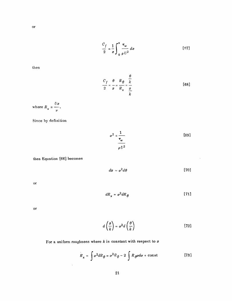
[171
Cf
2
RO k
RX[68]
12 -
pw
pU2
[69]
dx = a2dO [701
[71]
[72]
11fll"',u
= o2d
[731

x =$-( ) O2d+ const-= a 2 d - 2 - f- ado + const
k k k k
The general case of the frictional resistance of a rough plate is to be now considered
wherein B1 or B2 is an unspecified function of k*. All other cases like that of the fully roughregime or the quasi-smooth regime are then special cases.
Inserting the relation - from Equation [12] into the relation for - from Equation [62]k k
and integrating by parts repeatedly results in
ado AD=
A
a2
1-
where
(B 2 B2 B2) 2AD 2 [ 14AB)+ .B2" + B2 - - + . . .] _ +L--A a a
+ a 2 d- -do + const
dB2
d (In k*)
d2B2B22 d (In k*) 2
and
[76]
[77]
Then from Equation [741
x 8 D
k{ D
B2 A + B 2 +
a _ a - 2 A la \ 1
2AD 2 [ 1 (A B2 )S. 1 + - - + ...
or a
[781
Jf,3 2+a2a-3 2 2 d+2f do + const
tr
Also since by definition
R x-SRx Rx k
k aok* u 3I-
av
[79]
~auMaa~l I II I - -a~IL111 Is I-----
[74]

[80]
+a 2 - 1 a-2 faoada + 2 J da + const
xHience from Equation [68] it is seen that Cf is a function of Rx and/or k in terms of parameter
a. When a is eliminated, logarithmic resistance formulas result. To arrive at a relation be-
tween Cf and a, Equations [68] and [73] or [74] are combined to give after neglecting the con-
stant of integration
C 2 JROada1 Cf 1a - [811
a2 2 \ 2 )
,f a da1 Cf k
a2 2 a2k
[82]
0 0The expressions for f a da and k- from Equations
tion [82] to give with a 2 and p2 neglected:
[75] and [62] are inserted into Equa-
SC 2A 2AB 2 2A2 82 D2_1 1-- + +2 B'+B --2 "
a2 2 a 2 3 2 A
Through reiteration a is replaced by Cf within the brackets so that
S 1 -2A 2+ 2A A+B -+ . ..a2 2 2
and by the binomial expansion
1= 2 (AA +l f) +. . .C-f[1 A( -f)"+ + B" -ra 2 ) (2/-
+...] [831
[841
[851
Equation
R -Rx=
" ""~"'
[78] becomes then
SDB2' A B ) ( 'A -Da 22 a-2ADa 1 12 B;+B.- +. + 2AD2 1+ - +..
I a o2 A o
~""II - "'

and by inversion
a= I +A +A A ) ()+... [Se]
8
Now, after substituting for k from Equation [12] and eliminating a2, 132' and the constantX k
of integration, -in Equation [78] is written in logarithmic form ask
a a B3 B2 1 2In + In D - In 1- - A+- -+In... [87]
k A A A D a
Substituting the appropriate expressions for a from Equations [85] and [8,] and expanding the
logarithm of terms close to unity into a, series results in
- 1 1 A 92 B 3 B2In- ±, = _ +- + B /-+ 1 - - +ln [88]k A /Cf (/ 2 D, 2 A A
wherein terms of higher order than /'have been neglected. Inserting the expression for -1 f k
from Equation [79] and - from Equation [85] into [88] producesa
V2 1 1 2 A B3 B1ln R, C = -- - - + B 2 ) \ +1- + In 2D1 [89]
,quations [88] and [89] represent logarithmic resistance formulas for the general case of con-stant k* since B1 and B2 are functions of k*. Separate logarithmic formulas are obtained fromEquations [88] or [89] in the cases where B1 or B 2 is analytically defined in terms of In k*.
FULLY ROUGH REGIME
In this case the roughness effects have become strong enough to eliminate the laminar
sublayer and make .?2 constant. With B2 = B2 ,R and B2 = 0, Equation [88] reduces to
- 1 1 (A D2 B3 B2,RIn - - + - + 1 + In V2 D 1 [90]
k A VC, - 2 2 D, A A
If the term involving fis linearized with respect to
or
/= C1 +C [91]N/Cf
i nr)~n*r~ I II ~I1P~ll~e~llill~llll-- ~h II- ^~IICI

then Eauation [90] becomes in common logarithms
x 1loglo k v= + N1
where
11 2.3026
and
1
2.302(_ D2 C1
Di ) N/2 -
A(B + o
A lo°
Furthermore, if loglo Cf
or
then Equation [92] becomes
1is linearized with respect to -
C 4lo10 C = C3 +
"U;
0 2.log - 2 +1
k
M2
lgf o 2 2
2
M2 =M1 2
C3N2 = 1 2
[96]1
[97]
[98]
[99]
QUASI-SMIOOTH REGIME
Quasi-smooth flow is effectively that of a smooth surface; B1 being constant and equal
dB 1to B1 , and dink*- 0.
[92]
V2 A D2 )C2-- -2- - [93]
-v D1 [94]
[95]
where
and

Since, from Equation [9]
, d B2 d B[100]
2 dlnk* dlnk*
Equation [89] reduces to
+ 1 A D2 B3 Bl,sIn Rx C f + 1 D + In 2 D1 [101]A D ,2 0 A A
If the term involving VC is linearized with respect to-- as in Equation [91], Equa-
tion [101] becomes in common logarithms
M1
logo Rx C =- + N, [1021
where M1 is given by Equation [93] and
S B2 ,R - B 1,sN = N + 2.3026A + oglo [1031
Equation [102] is the well-known Karman-Schoenherr formula which is derived in Reference
20 by a somewhat different procedure.
If loglo Cf is linearized with respect to-as indicated in Equation [95], Equation
[102] becomes f
logto Rx - + N' [1041
or
Cf = [105]
(log1 0 RX - 2
where
M2= M1 C4 [106]
and
N2 = N1 - 3 [1071
ENGINEERING ROUGHNESS
From extensive tests on commercial pipes the behavior of the irregular roughness ofthe surfaces resulting from manufacturing processes, termed here engineering roughness, hasbeen found to be quite different from that of the artificial sand roughness of Nikuradse.
~164~ - I _ --rr r~---------y~-, - -~- I -------- II~

Whereas B2 has a maximum value for the Nikuradse roughness, B2 has a gradual monotonic
variation for engineering roughness as shown in Figure 1. Colebrook"1 with the aid of White
fitted this variation of B2 with the following formula whicn in the notation of this paper can
be expressed as
B2 = B2,R - Aln 1 + [1081
where
X = exp (B2, R - B1,s [109]
It is seen that for k* -~ -, 8 2 - B2,R'
Furthermore, with Equation [9], [108] becomes
B = Bis - A In 1 + - [110]
Then for k* -+ 0, B1 - B1, s . Consequently the relation for engineering roughness is asymptotic
to both the quasi-smooth regime and the fully rough regime.
To obtain a logarithmic resistance formula for engineering roughness from Equation
[891, the procedure is as follows:
From Equation [108]
[11111k*1+-
Now from Equations [79] and [85]
1 + =1+ 1-A +... = 1+
_-
x)2k Iv2X-k
ARx) Cf
A-k
_
k
[1121
Using Equations [110], [1111, and [112] in [89] results in
1 1 1r2 1 /A D2 ) B3 B1
SR X A K 2Xf D,[ A1
[113]
I '--III I Ii

1If the term containing V7 is linearized with respect to--as in Equation [91], Equa-
tion [113] becomes in common logarithms VZ7
- logo + - + Ni [1141
where M1 is given by Equation [93] and N1 by Equation [1031.
Equation [114-] reduces to the case for smooth flow, Equation [102], when
1 1-, 0 and to the case for the fully rough regime, Equation [92], when - -+ 0.
In a less rigorous fashion an explicit expression between Cl and Rx and k may be
written which agrees in the limits with Equation [104] for the quasi-smooth regime and with
Equation [96] for the fully rough regime or
log - +----- = - + N2 [115]
where M2 and N2 are given in Equations [106] and [107],
log,0 0 y - N2 [1161
and
2m = [117]
APPLICATION OF THE GENERAL LOGARITHMIC RESISTANCEFORMULA TO ARBITRARY ROUGHNESS
PREPARATION OF RESISTANCE DIAGRAMS FROM RESISTANCECHARACTERIZATIONS
If the resistance characterization is known for an arbitrary roughness, e.g., B1 or B2has been found empirically as a function of k*, the procedure for preparing a resistance dia-gram for flat plates, Cf as a function of Rx and z/k, is as follows:
The general logarithmic resistance formula, Equation [89], is restated in common log-arithms and Equation [100] substituted for B2
*N~ I 11 I"M1,11-ill , , W FNWW4.0 11 No"---^- -- - -_

S 1 (A 92 1 _B _1 B B1g10 X Cf 2302 A 21
oglo R I - 2.3026A - 2.3026 -2 D, 2.302 dloglok * 2.3026 A A
[1181
+ log 0o 2 D,
d B1
Since B1 and d are functions of k* and A, B3, D1, and D2 are constants, Equationdloglok*
[118] represents the variation of Cf with Rx for constant k*. A rapid method of plotting Fqua-
tion [118] is to relate it to smooth resistance so that for the same value of C the difference
in Rx is
B1 , -B 1
logl 0 Rx - l oglo Rxs 2.3026 A [119
dB
where the effect due to is neglected and the subscript s refers to the smooth line.dloglok*
Consequently the resistance line of constant k* for the rough case is offset from the smooth
line by a constant amount in the direction of log 10 Rx .
To determine the resistance lines of constant x/k from the lines of constant k* the
following procedure is used:
Since by definitionx
R k* a- [1201x k
the insertion of the relation for a from Equation [86] produces
Rx = k* - 1C + A +[211
Taking the common logarithm of Equation [1211 and expanding the logarithm of the series in
parentheses results in
loglo Rx = logok* + loglo + .3 + loglo [122]
wherein terms of higher order than /f have been neglected. Hence for a given k* and x/k
the intersection of Eauation [122] and [119] at a specified k* gives a point on the line of
constant x/k. A rapid way of plotting other lines of Equation [122] is to relate them to any
plotted line of Equation [122] at constant Cf or
- --Ii

log 10 Rx, 2 - log 1 0 R 1 = loglok - loglok' + logl - log123
where subscript 2 refers to the new line and subscript 1 to the line already plotted. Hencethe various plots of Fquation [122] are offset by constant amounts in the direction of loglo0 R.
This procedure was utilized in preparing the resistance diagram for sand roughness inFigure 7 from a graphical representation of B1 and k*.
RESISTANCE CHARACTERIZATIONS FROM PLATE TESTS
To characterize the resistance qualities of an arbitrary roughness requires the deter-mination of B1 or B2 as a function of k*. Measurements of total resistance of flat plates withan arbitrarily rough surface can only give values of C. against Rx for different lengths x, theroughness parameter k having only meaning for a particular roughness configuration. Henceto compare the resistance characterizations of different roughnesses from measurements oftotal resistance of flat plates, it is necessary to use the following procedure:
A new parameter x* is introduced where
*1Ux* - [1241
so that by definition
k* /k [125]x/k
or
logok* = loglox* - loglo k [126]
Then the single parameter variation of B1 with k* is replaced by a two-parameter variation ofB1 with x* and a/k. Consequently when B1 is plotted against loglo x*, a family of curves re-sult for different values of x/k which are offset by constant amounts of the differences inlogo1 0 x/k.
B1 is determined from the general logarithmic resistance formula [118] and from thefact that for constant z/k
d B1 d B1
dloglo0 k* dloglo* [127]
2 AoA D2 dB 20,
Of 2\ D1 2.3026 dlogloa* to x C
lil*(XII*~ _* 1 11-----~1(* -- I I ---CSI

7
4 X310
0 x10
Figure 7 - Resistance Diagram for Rough Plates with Sand Roughnessand Engineering Roughness.yo4 N b oSand RoughnessEngineering Roughness Rogn
and Engineering Roughness

or relative to the smooth line for the same Cf
A dB1 fB =Bs dlo - 2.3026A (loglo Rx - Rx,s)1,s 2.3026 dloglx,*V2f
dB1The small effect due to can be evaluated by iteration.
dloglox*
Since by definition* =
x*
[129]
[1301
then substituting for 1/a from Equation [85] and manipulating the logarithm of the series gives
logloz* = loglo Rx + log - 2.3026 [131]C 2
Hence B1 and x* can be obtained from test data of C against Rx .
For the same roughness k and different lengths of plate x, plots of B1 against loglox*will be represented by curves offset by a constant amount given by the logarithm of the ratioof the lengths of the plates. Hence, if the similarity laws hold, the curves can be collapsed
to a single line by parallel shifts of the curves in the z* direction.
A resistance characterization was obtained from the data of 21-foot friction planescoated with Mare Island hot plastic paint as shown in Figure 8. For comparison the curve ofengineering roughness, Equation [110], is plotted for x/k = 1 x 10s . The difference in curva-ture between the two graphs is evident.
0.3 0.4 0.5 0.6 0.7 0.8 0.96
Log x*= Logu10 0
i
Figure 8 - Resistance Characterization of Roughness fromFlat Plate Resistance Data
- I 1 ,_I I I

PREDICTION OF FULL-SCALE RESISTANCE FROM PLATE TESTS
The general logarithmic resistance law provides a means of extrapolating data from
test planks with arbitrary rough surfaces to full-scale lengths. The test data are in the form
of Cf against log Rx at constant z/k, k being unknown. A representative plot for Mare Island
hot plastic paint 2 1 is shown in Figure 9. The problem is to obtain a plot of Cf against log Rx
for different lengths of flat plates with the same roughness in order to predict the full-scale
resistance of ships having that roughness.
According to the similarity laws there is a unique relationship between B1 and k*
characteristic of the roughness configuration. Hence each point of the test data or faired
test curve represents a value of B1 or k*. This is illustrated by point P1 in Figure 9 where
a line of constant B1 or k* is drawn through it by means of Equation [119] which simply re-
quires that a constant distance from the smooth curve be maintained in the logloRx direction.
The next step is to locate a point on this line which corresponds to the desired length of
plate.
First from Equation [131] a line of C against Rx at constant x* is drawn using any
convenient value of x*. From Equation [131] again it is seen that at constant Cf the differ-
ence in lines at different x* is given by
logl 0 Rx, 2 - logl 0 Rx,1 = logl 0 X - logl 0 X [132]
Since by definition
X* k*- [133]k
Equation [132] becomes for constant k* and k
@2log 10 Rx, 2 - log1 0 R,1 = log 1 0
134
Consequently point P2 for the new length x2 is located by a line which is at a distance of
log 10 2 from P1 and drawn a constant distance from the reference line for constant x*. This
1
process is repeated for enough points from the test data to draw the predicted line for the
desired length as illustrated in Figure 9.
If a representative sample of the rough surface can be obtained on a test plate, it is
then possible to make full-scale predictions for any arbitrary roughness configuration with-
out regard to geometrical characterization.
11

0.8
0.6
0.4
0.2
4 ,40
08 toglo g0.6 1 , ooo
I "/I
So ft Friction Plane08 T0.s -Cntn Constnt x
Reference Line tant x3 of Constant x ons x
c 0.80 ..,Constant B. or k*
0.6
0.40 -
S0.2 \ o -Constant xS 0.2- 400 Plate
a 0.8
Mare Island Hat Plastic
0.60.4
0.2
S 0.2 0.4 0.6 0.8 0.2 0.4 0.6 0.8 0.2 0.4 0.6 0.8 0.2 04 0.6 0.86 7 8 9 10
Reynolds Number, logR x
Figure 9 - Resistance Prediction Diagram for Rough Plates

LOCAL SKIN FRICTION COEFFICIENTS AND SHAPE PARAMETERS
GENERAL
In the calculation of turbulent boundary layers in pressure gradients to obtain the vis-
cous resistance or separation point of foils and bodies of revolution, 2 2 ' 23 relations are re-
quired for the local skin friction and shape parameter as functions of momentum thickness.
For rough surfaces in general the local skin friction is expressed as
= = - f (Ro, O/k) [135]02 2 PU 2
and the shape parameter H as
H = f(Ro, 0/k) [136]
From Equations [11] and [61] the local skin friction is expressed implicitly as
R0 = D, 1- exP A (a-B 3 -B) [137]
or from Equation [12] and [62]
0 O D2- 1 -- exp B-B) [1381k a Da)l a
where a.1 , 01, a2, and 02 have been neglected. Logarithmically Equation [137] becomes
1 2 83 1 D2 wIn Ro = + In D - [1391
A , A AP 101U2
and Equation [1381 becomes
0 1 U2 3 2 w D2 rwIn -= + In D + In [1401 -
- -~j~nD, la - ---y~---- [140]k A -W A A p U2 1 p 2
wherein one term has been retained in the series expansion of In 1- . Equations
[139] and [140] represent the general case with B1 and B2 as functions of k*.
In the case of shape parameter H, Equation [64] is simplified to
H Di D1 U2H - a I =- [1411H-1 D2 D2 Vrw

by dropping a 1 and 1 1.
FULLY ROUGH REGIME
Since in the case of the fully rough regime B2 is constant, B2 = B2,R Equation [1401
is then
i n U 2B3 2, R
A A+ In D, --
Di CPU 2
If the term involving - is linearized with respect
= + a 2
then Equation [142] becomes in common logarithms
[142]
to or
[143]
= O~/-" + Pr w
1 a2 2
1 2.3026A 2.302AD1
al D2+ loglo D12.3026D1 1
Furthermore, if loglo0 is linearized with respectPC72'
log 10 = a3
to or
+aAFy
w [147
Equation [144] becomes approximately
log 1lo 0 =2V + P2Sw[1481
where
[144]
and
[1451
SB3 -0 2 , R
2.3026A[1461
1IL*~n*l I I - - I-l-C-- II Irl -, I ------------LI ---- ~-
A1U
loglo ( -2
k ~f61V rw

[1491
where
and
w 02
PU 2 oglo
02 = 01 + a4
P2 =1 + a3
In the case of H, the substitution of Equation [148] into [141] produces
H-1( D2)0 D1 P2
log10 k D2 O
[150]
[1511
[1521
QUASI-SMOOTH REGIME
In the case of the quasi-smooth regime B1 is constant, B1 = B1 ,s , and Equation [1391
becomes
+ In D - --rCPU 2
If the term containing is linearized with respect to
w 02
[1531
as in Equation [143],
[1541
[1551
where 01 is given by Equation [145] and
1 / B3 B1, s
0 A 'rw A A
pU 2 (log R 0 -P )2
B2 ,R -Bl,sS= + 2.3026A
[156]1
-

An equation of the form of [155] was first derived by Squire and Young 2 4 for smooth surfaces.
The shape parameter H for quasi-smooth regime becomes after substituting Equation
[154] into [1411
H Di D, P,DO )logO 0 RO
H- 1 , 2 D 21
[157]
ENGINEERING ROUGHNESS
In the case of engineering roughness, B1 is analytically defined as a function of k*
by Equation [110] which, since k* is by definition
R8 wk* =
O/k U2[1581
is written
Bi = Bl's - Al I +xf!k ,212 [159]
For B1 given by Equation [159], Equation [139] becomes
7wP_ Y 2 1 12 B3 B1.
1-_+ - + InRO X O/k A + A A
2 7DD1 - 21 rpU
2
If the term containing - is linearized with respect to - as inSpU"w
(1601
Equation [143],
Equation [160] is then in common logarithms
- log1 + -
0 RO X O/k= O1V- + P,
where 01 is given by Equation [145] and P1 by [156].
Since no simple expression for H can be obtained from Equations [141] and [161], it
is necessary to retain - as the intermediate parameter for calculating H.pU
2
[1611
"~ ~aa aar-- ---~-- ---~ -r~19-~-. I r mr

PREPARATION OF LOCAL SKIN FRICTION COEFFICIENT AND SHAPE PARAMETERDIAGRAMS FROM RESISTANCE CHARACTERIZATIONS
Where B1 is empirically stated as a function of k* for any roughness configuration, a
convenient method of preparing a diagram of and H plotted against R and O/k is by com-
pU 2
parison with - and H for the smooth case.pU 2
w
From Equation [139] for the same value of - and in common logarithms
pU2
B1, s - B1log 10 R - lglo0 RO, ,s 2.3026A [162
Consequently, the resistance line of constant k* or constant B1 for the rough case is
offset from the smooth line by a constant amount in the direction of loglo RO.
To determine the resistance line of constant O/k from the lines of constant k* the pro-
cedure is as follows:
Since by definition 0 r2R k 0 k* [1631
Ofor
loglo R0 = logo10 O/k - loglo0 - + log 10 k* [1641
Hence for a given k* and O/k the intersection of Equations [162] and [164] gives the
desired point. A rapid way of plotting other lines of Equation [164] is to relate them to any
Irwplotted line of [164] at constant - or
pU2
log 1 0 R0,2 - log 0o R0 1= log10 (0/k)2 - log1 0 (0/k)1 + loglo k - log 10 k
[1651
The various plots of Equation [164] are then offset by constant amounts in the direction
of log 10 Ro. ilw
The procedure is the same for H since H is solely a function of - from Equation
[1411. PU2
milli

PREPARATION OF LOCAL SKIN FRICTION COEFFICIENT AND SHAPEPARAMETER DIAGRAMS FROM PLATE TESTS
-wTo prepare diagrams of - and H from total resistance results for an arbitrary rough-
pU 2
ness configuration, the following method may be employed:
From total resistance tests of a representative sample of a particular roughness the re-sults are given in the form of Cf = f (Rx, x). The objective of the analysis is to obtain
Tw-, H = f(RO, 0). From Equation [84] approximatelypU 2
U2 2(1-2A [166]
and from Equation [68]
1
and
0 2 X Cf [168]
To obtain lines of constant 0, a line is first drawn at a fixed distance in the logR0direction from the smooth curve for each data point which corresponds to a lind of constantk* in accordance with Equation [1621. Then to locate the point corresponding to the desired
.wvalue of 0 use is made of Equation [165] wherein for the same - , k*, and k
pU2
log1 0 RO,2 - Ogl1 0 R8,1 = log 1 0 92 - log 10 01 [169]
The reference line for using the above is from Equation [164]
loglo RO = - loglo, + constant [170]
the constant is any value convenient for plotting.
The values of H of the arbitrary roughness are calculated from Equation [141] wherein
H = 1 [1711D2 7w
1-- -
I1 pU 2
The remainder of the procedure for determining H=f(Ro, 0) is the same as that for -.pU 2
"-~ ---- I-- I...

NUMERICAL RESULTS
The experimental difficulties in boundary-layer measurements have resulted in consid-
erable discrepancies in numerical values of constants among investigators in the field. 25
Although future tests will thus in all probability lead to somewhat different values, the numer-
ical results gathered and calculated by Landweber"1 have been judged to be as reliable as
any and have been used to evaluate the factors derived in this report. For convenience of
reference, the numerical values are listed in Table 3.
TABLE 3
Numerical Values of Factors
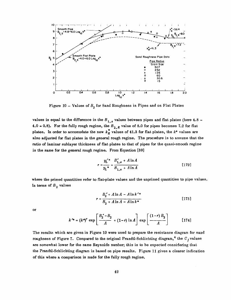
Since the sand roughness values of Nikuradse t were obtained from pipe flow, some
adjustment is needed for application to flat plates. The values of B2 of Nikuradse were ob-
tained by using a value of 5.75 for 2.3026A which differs from the value of 6 used by
Landweber for flat plates. Consequently the velocity profiles of Nikuradse were replotted
and new B2 values for pipes were obtained using the slope of 6 as shown in Figure 10.
The B2 values are converted to those for flat plates by assuming that the difference in such
tHere k refers to the size of the sand grains.
Factor Value Source Factor Value Source
a1 0.0625 Calc. m 1.076 Eq. [117]
a2 -7.57 x10- 4 Calc. M1 0.242 Eq. [93]
a3 -1.082 Calc. M2 0.262 Eq. [981
a4 -1.306x10 2 Calc. M 0.282 Eq. [1061
2.3026 A 6 Ref. 18 N1 -0.661 Eq. [94]
A 2.6 Ref. 18 N; 0.023 Eq. [1031
B,, s 4 Ref. 18 N2 0,215 Eq. [99]
B2,R 7.2 Fig. 10 N 1.729 Eq. [107]
B3 2 Ref. 18 01 0.1689 Eq. [145]
C, 0.105 Calc. 02 0.1558 Eq. [150]
C2 -2.5x10 - 3 Calc. P1 - 1.169 Eq. [146]
0 3 -1.752 Calc. P,' -0.636 Eq. [156]
C4 -0.04 Calc. P2 -2.251 Eq. [1511
Dz 3.499 Ref. 18 v 24.66 Eq. [1161
D2 23.23 Ref. 18 X 3.42 Eq. [109]
RWIA N 1 1
I I
Smooth Pipe k = 564
98 S=4.8+6.OLog k* x
7 -8 8- -
k -41.36-R
B2 5 , B2 .+60 Log 10k Sand Roughness Pipe Data
- I Pipe Radius4 Grain Size
* 5073 0 252
x 126o 60
2 . 30.6V 15
0 0.2 0.4 0.6 0.8 1.0 1.2 1.4 16 1.8 2.0Logl0 k*
Figure 10 - Values of B2 for Sand Roughness in Pipes and on Flat Plates
values is equal to the difference in the B 1 ,. values between pipes and flat plates (here 4.8 -
4.0 = 0.8). For the fully rough regime, the B2,R value of 8.0 for pipes becomes 7.2 for flat
plates. In order to accomodate the new k R values of 41.3 for flat plates, the k* values are
also adjusted for flat plates in the general rough regime. The procedure is to assume that the
ratio of laminar sublayer thickness of flat plates to that of pipes for the quasi-smooth regime
is the same for the general rough regime. From Equation [39]
YL'* B + AInAr = [1721
YL* Bs + AlnA
where the primed quantities refer to flat-plate values and the unprimed quantities to pipe values.
In terms of B 2 values
B2 + AInA - Alnk'*r = [173]
B2 + AlnA - Alnk*
or
* = (k*) exp 2 +(1-r) InA exp A) B[1741A A
The results which are given in Figure 10 were used to prepare the resistance diagram for sand
roughness of Figure 7. Compared to the original Prandtl-Schlichting diagram, 4 the Cf values
are somewhat lower for the same Reynolds number; this is to be expected considering that
the Prandtl-Schlichting diagram is based on pipe results. Figure 11 gives a clearer indication
of this where a comparison is made for the fully rough regime.
.uunal-. - --y -- I ------- - I II.--.^ ---- X II I I-I 1 111 11 II 11 11--~-cl,.-
I I I

0 1 1 I 1 I I I I I I I I I2 3 4 5 6 7 8 9
Logl0 k
Figure 11 - Coefficients of Total Resistance for the Fully Rough Regime
2 3Log-o
10 k
1.8
1.7
1.6
1.5
1.4
1.30
I.2 o0CL
Cn
1.0
Figure 12 - Local Skin Friction and Shape ParameterRough Regime of Flat Plates
for the Fully
For the total resistance of smooth plates, the new M1 value of 0.242 is identical to that
of the Schoenherr formula and the new N1 value of 0.023 is close to that of zero for the
Schoenherr formula.
Finally, for the fully rough regime Figure 12 shows a comparison of local resistance
coefficients and H values from Equations [144] and [141] to those of Scholz 2 6 obtained by a
simple power-law analysis of the Prandtl-Schlichting formula. The local resistance coefficients
compare well but the H values show a large difference which is due to the improper power-law
analysis of Scholz.
in
219

ACKNOWLEDGMENT
The author wishes to express his appreciation to Mr. Ralph D. Cooper for his critical
review of this report.
REFERENCES
1. Prandtl, L., "The Mechanics of Viscous Flows," Vol. III of "Aerodynamic Theory,"
W.F. Durand, ed., Julius Springer, Berlin (1935).
2. Von Karman, T., "Mechanical Similitude and Turbulence," NACA TM 611 (Mar 1931),
(Translation from Nachr. Ges. Wiss. Gottingen, 1930).
3. Von Kirmin, T., "Skin Friction and Turbulence," Journal of the Aeronautical Sciences,
Vol. 1, No. 1 (Jan 1934).
4. Prandtl, L. and Schlichting, H., "The Resistance Law for Rough Plates," David Taylor
Model Basin Translation 258 (Sep 1955), (translation from Werft-Reederei-afen, Jan 1934).
5. Nikuradse, J., "Laws of Flow in Rough Pipes," NACA TM 1291 (Nov 1950), (translation
from VDI - Forsch. 361, 1933).
6. Squire, H.B., "Reconsideration of the Theory of Free Turbulence," Philosophical Mag-
azine, 7th Series, Vol. 36, No. 288 (Jan 1948).
7. Laufer, J., "Investigation of Turbulent Flow in a Two-Dimensional Channel," NACA
TN2123 (July 1950) or NACA Report 1053 (1951).
8. Batchelor, G.K., "Note on Free Turbulent Flows, with Special Reterence to the Two-
Dimensional Wake," Journal of the Aeronautical Sciences, Vol. 17, No. 7 (Jul 1950).
9. Schubauer, G.B., "Turbulent Processes as Observed in Boundary Layer and Pipe,"
Journal of Applied Physics, Vol. 25, No. 2 (Feb 1954).
10. Clauser, F.H., "Turbulent Boundary Layers in Adverse Pressure Gradients," Journal
of the Aeronautical Sciences, Vol. 21, No. 2 (Feb 1954).
11. Millikan, C.B., "A Critical Discussion of Turbulent Flows in Channels and Circular
Tubes," Proceedings of the Fifth International Congress for Applied Mechanics, Cambridge,Mass. (1938), John Wiley and Sons, New York (1939).
12. Rotta, J., "Das in Wandnlihe g'Ultige Geschwindigkeitsgesetz turbulenter Str8 mungen,"
(The Velocity Law Which Is Valid in the Vicinity of the Wall for Turbulent Flows), Ingenieur-
Archiv, Vol. 18, No. 4 (1950).
13. Hudimoto, B., "A Brief Note on the Laminar Sub-Layer of the Turbulent Boundary Layer,"
Memoirs of the Faculty of Engineering, Kyoto Univ. (Japan), Vol. 13, No. 4 (Oct 1951).
m----------a -r~- rs~ --1~------------ ---- --~-- -- - x-- -LI I-----~s~ll-

14. Hama, F.R., "On the Velocity Distribution in the Laminar Sublayer and Transition
Region in Turbulent Shear Flows," Journal of the Aeronautical Sciences, Vol. 20, No. 9
(Sep 1953).
15. Van Driest, E.R., "On Turbulent Flow Near a Wall," North American Aviation Report
AL - 2077 (Oct 1954); also, 1955 Heat Transfer and Fluid Mechanics Institute at Univ. of
Calif., Los Angeles; also, Journal of the Aeronautical Sciences, Vol. 23, -No. 11 (Nov 1956).
16. Laufer, J., "The Structure of Turbulence in Fully Developed Pipe Flow," NACA TN
2954 (Jun 1953).
17. Goldstein, S., "A Note on Roughness," (British) Aeronautical Research Committee
R & M 1763 (Jul 1936), Vol. 51 (1937).
18. Landweber, L., "The Frictional Resistance of Flat Plates in Zero Pressure Gradient,"
Transactions of the Society of Naval Architects and Marine Engineers, Vol. 61 (1953); also,
"Der Reibungswiderstand der Lingsangestr*mtenebene Platte," Jahrbuch der Schiffbautech-
nischen Gesellschaft, Vol. 46 (1952).
19. Colebrook, C.F., "Turbulent Flow in Pipes, with Particular Reference to the Transi-
tion Region between the Smooth and Rough Pipe Laws," Journal of the Institution of Civil
Engineers, Vol. 11 (1938/39).
20. Granville, P.S., "The Viscous Resistance of Surface Vessels and the Skin Friction
of Flat Plates," Transactions of the Society of Naval Architects and Marine Engineers,
Vol. 64 (1956).
21. Couch, R.B., "Preliminary Report of Friction Plane Resistance Tests of Anti-Fouling
Ship Bottom Paints," David Taylor Model Basin Report 789 (Aug 1951).
22. Granville, P.S., "A Method for the Calculation of the Turbulent Boundary Layer in a
Pressure Gradient," David Taylor Model Basin Report 752 (M'ay 1951).
23. Granville, P.S., "The Calculation of the Viscous Drag of Bodies of Revolution,"
David Taylor Model Basin Report 849 (Jul 1953).
24. Squire, H.B. and Young, A.D., "The Calculation of the Profile Drag of Aerofoils,"
(British) Aeronautical Research Committee R & M 1838 (Nov 1937).
25. Hama, F.R., "Boundary-Layer Characteristics for Smooth and Rough Surfaces," Trans-
actions of the Society of Naval Architects and Marine Engineers, Vol. 62 (1954).
26. Scholz, N. "Uber eine rationelle Berechnung des Stromnungswiderstandes schlanker
K~rper mit beliebig rauher Oberflh'che," (On a Rational Calculation of the Flow Resistance of
Slender Bodies with Arbitrarily Rough Surfaces), Jahrbuch der Schiffbautechnischen Gesell-
schaft, Vol. 45 (1951).

-- ,-% '"N"m " oll" 0 - . 11, 1 1 M 1

Coples
17 CHIIIISIPS, Library (Code 312)5 Tech LiSaryI Tech Asst to Chief (Code 106)2 Appl Sci (Code 37012 Design (Code 410)3 Preh- Cesren rCode 420)
I Dr. 1. .lversteln3 Submarines (Code 525)1 Propellers P Shafting (Code 554)
5 CHIIORD, Underwater lrd (Relia)1 Dr. A. 'lllerI r'r. P.A. Eleers
3 CFB'AER2 Aero 7 Hydro Br (DE-3)1 Appl Math Dr
4 ihRI 'atematics (Code 432)2 fechanic (Code 438)1 Undersea *artare (Code 466)
2 Dir, USIRL
4 CDR, US'IOL, 'ecc Div
2 CfiH, USOfiTS, China Lake, Calif.1 Inderwater 0id nlv, Pasadena Annex
I NAVSHIPYD .APE
1 NIAVSHIPYD %ORVA
2 NAVShIPYD PTSAHI Capt L.A. Rupp
1 CDR, USIPG, Daklpgen, Va.
1 rf DIP, US::USL, "!ew London, Conn.
2 CO, US':UOS, Design Section, lewport, R.I.
1 CO, USNATC, Patuxent River, Md.
I Supt, USN Postgfad Sch, Monterey, Calif.
I Dir, anlne Physical Lab, USIIEL, San Diego, Calif.
1 Chrm, Defense Science Board
I Dir, Aero Res Lab, Wringht Air Dev CtrrightlMPatterson AFS, 0.
I Tech Info Div, Library of Congress
2 Chief, ASTIA Document Clr, Arlington, Va.
I Dir, Balltic Res Lab, Aberdeen Proving Ground,Aberdeen, Pd.
2 Der of Res, Engr Res & Dev, Fort P.evor, Va.
1 Dir, Tech Info Br, Aberdeen Proving Ground,ALerdeen., d.
1 Dir, NACA
3 PIr, Langley Aeo Lab, Langley AF, Va.1 Dr. 4.F. von Doenhoff1 VLr. 1N. Tetervin
2 Dir, Lewis FI Propul Lab, Cleveland, 0.
NAVYDCPPO PNC WASH DC
INITIAL DISTRIBUTION
Copies
2 Dir, Ames Aero La,, Moffett Field, Calif.
I Dir, nak Ridge altl Lab, Oak Ridge, Tenn.
2 Chief, ratl Hydr Lab, fatl BoStands
2 Hydro Lab, Attn Exec Corn, CIT, Pasadena, Calif.
1 Dir, lost of Engin Res, Ulniv of Calif, Berkeley, Calif.
2 Colorado State tnir, Di, Hydr Lab, FL Collins, Colo.1 'Ir. B. Chanda, Dept of Civ Engrn
2 Dir, Iowa Inst of Hydr Res, State (lnlv of Iowa, Iowa City,Ia.1 Dr. L. Landweber
3 Dir, Inst for Fluid Dynamics Appi ath, Unlv of ilarylandCollege Park, 'Id.I Prof. J.'. Weske
1 Dr. F.R. lama
2 Dir, Exper Nav Tank, Dept NAE, Umny of hchigan,Ann Arbor, lich.
2 Dir, ETT, SIT, Hoboken, r'.J.1 Dr. J.P. Breslln
Ori, Jet Propul Lab, CIT, Pasadena, Calif.
1 Dir, Oefense Res Lab, Univ of Texas, Austin, Tex.
1 Dir, St Anthony Falls Hydr Lab, Untv of 'innesota,1linneapolis, Meinn.
2 Dir, (lRL, Penn State Univ, University Park, Pa.
1 Dir, tidwest Res Inst, Iansas City, Mo.
1 Dir, Robinson Model Basin, Webb Inst of Nav AiclhGlen Cove, L.I., N.Y.
2 'ead, Dept NAIE, MIT, Cambridge, Uass.1 Prof. AbkorwitZ
2 SIIPSHIPIr'SORD, General Dynamics Corp, roton, Conn.1 Electric "oat Division
2 N:ISB DDCo, 'ewport :ews, Va.I Sr Naval Architect
1 Sup, Hydr Lab
I Editor, Aero Engln Review, New York, N.Y.
1 Editor, Appl Mech Review, Southwest les Inst,San Antonio Tax.
1 Editor, Bibliography of Tech Reports, Office of Tech ServU.S. Dept of Commerce
1 Editor, Engin Inden, New York, N.Y.
I Editor, Mathematical Reviews, Brown Univ, Providence, R.A
2 Tech Library, Douglas Aircraft Co., Iec., El Segendo, Calif.,I Mr. A.I.O. Smith
2 Tech Library, North Amer Aviation, Inc., Downey, Calif.
I Dr. E.R. van Dnest
2 Dir, Aero Res Lab, 'elbourne, Australia
47
Copies
I Dir, Inst of Aemophysics, Univ of Tomnto, Toeoalo, Canado
3 NPL, Teddington, England1 Aem ODr2 Ship Div
1 Head. Aer Dept, Royal Aircraft Estab,Fambolourh, Hants, England
I Dr. S.L. Smith, Dir, BSRA, London, En2landi H. Lackenby
I Dir, Bassin d'Essals des Canes 6, Pans, France
I Dir, Societe Grenbloise d'Etudes at d'ApplicatonsHydrauliques, Grenoble, (Iske) France
I Office, :ati d'Etudes et de Recherches Airneaubque 3,Pans, France
1 Dr. J. Dreudenne, Dier, Insttut de Recherches de IaConstruction Navale, Pans, France
2 O.N.E.R.A., Service des Relations Extinees et de laDocumentabon, Chabllon-sous-Bagneux (Seme), France
S Prof. Dr. H. Schllchting, Instiltut gr Stromongs, Technlscke)ochschule, qraunschweig, ,enany
1 Gen. Ing. u. Pugliese, Pres., Insbtuto .az. per Studl ed
Eso.di Arch flay, Rome, Italy
I ir,Laboratorium Voor Aero-En Hydrodynamica, Delft,Naetherldands
1 Dr. f1. Lopez Acevedo, Jer, Canal de Fxpenanceas Hidlodina-micas, ladnd, Spain
1 Dir, flededand Scheepsbouwkundig Proestabon, Wageningen,Holland
I Dr. Hans Edstrand, Dir, Statens Skeppsprovningsanstalt,Goteborg, Sweden
S ODir, Libraly of Chalmers Unlv of Tech, Coteboeg, Sweden
2 Dir, Institut for Scliffbau der Universitat Hamburg,Hamburg, GermanyI Dr. K. Wlghaerdt
I Dr. H.W. Leeks, Hambuntische Schffbau-Versuchsanstalt,Hamburg, Germany
1 DiO, ARL, Teddinglon, England
~X~I_~ _______~____~_ ~ ____ _ __
L I

III, I oil NINIMPF" ml " 1 -1 NJ 1. 1, IN Nil 41 m IN III ON"

1-~MINIMU M - -Ili


0 754 21

A'
w kJ''
' . 1-~~ :
I '~~ ~ .
1~
.
Nr
3'...~-.2,,:I$
1
2'I
.15 ~~
H
I:~ .. : 1L
rl-ir3
s
;i
1--
,,
s:~I LL
1-c
MN 4-
Recommended