1
Algorithm-Based Fault Tolerance
for Fail-Stop Failures
Zizhong Chen and Jack Dongarra
Abstract
Fail-stop failures in distributed environments are often tolerated by checkpointing or
message logging. In this paper, we show that fail-stop process failures in ScaLAPACK matrix
matrix multiplication kernel can be tolerated without checkpointing or message logging. It has
been proved in the previous algorithm-based fault tolerance research that, for matrix-matrix
multiplication, the checksum relationship in the input checksum matrices is preserved at the end
of the computation no matter which algorithm is chosen. From this checksum relationship in the
final computation results, processor miscalculations can be detected, located, and corrected at
the end of the computation. However, whether this checksum relationship in the input checksum
matrices can be maintained in the middle of the computation or not remains open. In this paper, we
first demonstrate that, for many matrix matrix multiplcation algorithms, the checksum relationship
in the input checksum matrices is not maintained in the middle of the computation. We then
prove that, however, for the outer product version matrix matrix multiplcation algorithm, the
checksum relationship in the input checksum matrices can be maintained in the middle of the
computation. Based on this checksum relationship maintained in the middle of the computation,
we demonstrate that fail-stop process failures in ScaLAPACK matrix-matrix multiplcation can
be tolerated without checkpointing or message logging. Because no periodical checkpointing
is involved, the fault tolerance overhead for this approach is surprisingly low.
Index Terms
Algorithm-based fault tolerance, checkpointing, fail-stop failures, parallel matrix matrix
multiplication, ScaLAPACK.
✦
Zizhong Chen is with the Department of Mathematical and Computer Sciences, Colorado School of Mines, Golden, CO 80401-
1887. Email: [email protected].
Jack Dongarra is with the Department of Electrical Engineering and Computer Science, the University of Tennessee, Knoxville,
TN 37996-3450. Email: [email protected].

2
1 INTRODUCTION
As the number of processors in today’s high performance computers continues to grow,
the mean-time-to-failure (MTTF) of these systems are becoming significantly shorter
than the execution time of many current high performance computing applications.
Even making generous assumptions on the reliability of a single processor or link, it is
clear that as the processor count in high end systems grows into the tens of thousands,
the MTTF can drop from a few years to a few days, or less. For example, with 131,000
processors in the system, the current IBM Blue Gene L experienced failures every 48
hours during initial deployment [28]. In recent years, cluster of commodity off-the-
shelf systems becomes more and more popular. While the commodity off-the-shelf
cluster systems have excellent price-performance ratios, there is a growing concern
with the fault tolerance issues in such systems due to the low reliability of the off-
the-shelf components used in these systems. The recently emerging computational grid
environments [14] with dynamic computing resources have further exacerbated the
problem. However, driven by the desire of scientists for ever higher levels of detail
and accuracy in their simulations, many computational science applications are now
being designed to run for days or even months. To avoid restarting computations from
beginning after failures, the next generation high performance computing applications
need to be able to continue computations despite of failures.
Although there are many types of failures in today’s parallel and distributed systems,
in this paper, we focus on tolerating fail-stop process failures where the failed process
stops working and all data associated with the failed process are lost. This type of
failures is common in today’s large computing systems such as high-end clusters with
thousands of nodes and computational grids with dynamic computing resources. In
order to tolerate such fail-stop failures, it often requires a global consistent state of the
application be available or can be reconstructed when the failue occurs. Today’s long
running scientific applications typically tolerate such failures by checkpoint/restart in
which all process states of an application are saved into stable storage periodically.
The advantage of this approach is that it is able to tolerate the failure of the whole
system. However, in this approach, if one process fails, usually all surviving processes

3
are aborted and the whole application is restarted from the last checkpoint. The major
source of overhead in all stable-storage-based checkpoint systems is the time it takes
to write checkpoints into stable storage [23]. In order to tolerate partial failures with
reduced overhead, diskless checkpointing [23] has been proposed by Plank et. al. By
eliminating stable storage from checkpointing and replacing it with memory and pro-
cessor redundancy, diskless checkpointing removes the main source of overhead in
checkpointing [23]. Diskless checkpointing has been shown to achieve a decent perfor-
mance to tolerate single process failure in [20]. For applications which modify a small
amount of memory between checkpoints, it is shown in [9] that, even to tolerate multiple
simultaneous process failures, the overhead introduced by diskless checkpointing is still
negligible. However, the matrix-matrix multiplication operation considered in this paper
often modifys a large mount of memory between checkpoints. Diskless checkpointing
for such applications often produces a large size checkpoint. Therefore, even diskless
checkpointing still introduces a considerable overhead [20], [22].
It has been proved in previous research [19] that, for some matrix operations, the
checksum relationship in input checksum matrices is preserved in the final computa-
tion results at the end of the operation. Based on this checksum relationship in the final
computation results, Huang and Abraham have developed the famous algorithm-based
fault tolerance (ABFT) [19] technique to detect, locate, and correct certain processor
miscalculations in matrix computations with low overhead. The algorithm-based fault
tolerance proposed in [19] was later extended by many researches [1], [2], [3], [5], [21].
However, previous ABFT researches have mostly focused on detecting, locating, and
correcting miscalculations or data corruption where failed processors are often assumed
to be able to continue their work but produce incorrect calculations or corrupted data.
The error detection are often performed at the end of the computation by checking
whether the final computation results satisfy the checksum relationship or not.
In order to be able to recover from a fail-stop process failure in the middle of the
computation, a global consistent state of the application is often required when a process
failure occurs. Checkpointing and message logging are typical approaches to maintain
or construct such global consistent state in a distributed environment. But if there exists
a checksum relationship between application data on different processes, such checksum

4
relationship can actually be treated as a global consistent state. However, it is still an
open problem that whether the checksum relationship in input checksum matrices in
ABFT can be maintained during computation or not. Therefore, whether ABFT can
be extended to tolerate fail-stop process failures in a distributed environment or not
remains open.
In this paper, we extend the ABFT idea to recover applications from fail-stop fail-
ures in the middle of the computation by maintaining a checksum relationship during
the whole computation. We show that fail-stop process failures in ScaLAPACK [4]
matrix-matrix multiplication kernel can be tolerated without checkpointing or mes-
sage logging. We first demonstrate that, for many matrix matrix multiplication al-
gorithms, the checksum relationship in input checksum matrices does not preserve
during computation. We then prove that, however, for the outer product version matrix
matrix multiplcation algorithm, it is possible to maintain the checksum relationship
in input checksum matrices during computation. Based on this checksum relationship
maintained during computation, we demonstrate that it is possible to tolerate fail-stop
process failures (which are typically tolerated by checkpoting or message logging) in the
outer product version distributed matrix matrix multiplcation without checkpointing or
message logging. Because no periodical checkpoint or rollback-recovery is involved in
this approach, process failures can often be tolerated with a surprisingly low overhead.
We show the practicality of this technique by applying it to the ScaLAPACK matrix-
matrix multiplication kernel which is one of the most important kernels for the widely
used ScaLAPACK library to achieve high performance and scalability.
The rest of this paper is organized as follows. Section 2 explores properties of ma-
trix matrix multiplication with input checksum matrices. Section 3 presents the basic
idea of algorithm-based checkpoint-free fault tolerance. In Section 4, we demonstrate
how to tolerate fail-stop process failures in ScaLAPACK matrix-matrix multiplcation
without checkpointing or message logging. In Section 5, we evaluate the performance
overhead of the proposed fault tolerance approach. Section 6 compares algorithm-based
checkpoint-free fault tolerance with existing works and discusses the limitations of this
technique. Section 7 concludes the paper and discusses future work.

5
2 MATRIX MATRIX MULTIPLICATION WITH CHECKSUM MATRICES
In this section, we explore the properties of different matrix matrix multiplication algo-
rithms when the input matrices are checksum matrices defined in [19].
It has been proved in [19] that the checksum relationship of the input checksum
matrices is preserved in the final computation results at the end of computation no mater
which algorithm is used in the operation. However, whether this checksum relationship
in input checksum matrices can be maintained during computation or not remains open.
In this section, we demonstrate that, for many algorithms to perform matrix matrix
multiplication, the checksum relationship in the input checksum matrices does not pre-
serve during computation. We prove that, however, for the outer product version matrix
matrix multiplcation algorithm, it is possible to maintain the checksum relationship in
the input checksum matrices during computation.
2.1 Maintaining Checksum at the End of Computation
Assume Im×m is the identity matrix of dimmension m, Em×n is the m-by-n matrix with
all elements being 1. Let Hcm = [Im×m, Em×1]
T , Hrn = [In×n, En×1]. It’s trival to verify
Hcm = Hr
nT if m = n. For any m-by-n matrix A, the column checksum matrix Ac of A is
defined by Ac = Hcm ∗ A, the row checksum matrix Ar of A is defined by Ar = A ∗ Hr
n,
and the full checksum matrix Af of A is defined by Af = Hcm ∗ A ∗ Hr
n.
Theorem 1: Assume A is an m-by-k matrix, B is a k-by-n matrix, and C is an m-by-n
matrix. If A ∗ B = C, then Ac ∗ Br = Cf .
Proof:
Ac ∗ Br = (Hcm ∗ A) ∗ (B ∗ Hr
n)
= Hcm ∗ (A ∗ B) ∗ Hr
n
= Hcm ∗ C ∗ Hr
n
= Cf .
Theorem 1 was first proved by Huang and Abraham in [19]. We prove it here again to
show that the proof of Theorem 1 is independent of the algorithms used for the matrix

6
matrix multiplication operation. Therefore no mater which algorithm is used to perform
the matrix matrix multiplication, the checksum relationship of the input matrices will
always be preserved in the final computation results at the end of the computation.
Based on this checksum relationship in the final computation result, the low-overhead
ABFT technique has been developed in [19] to detect, locate, and correct certain pro-
cessor miscalculations in matrix computations.
2.2 Is the Checksum Maintained During Computation?
Algorithm-based fault tolerance usually detects, locates, and corrects errors at the end
of the computation. But in today’s highperformance computing environments such as
PVM [27] and MPI [26], after a fail-stop process failure occurs in the middle of the
computation, it is often required to recover from the failure first before the continuation
of the rest of the computation.
In order to be able to recover from fail-stop failures occured in the middle of the
computation, a global consistent state of an application is often required in the middle
of the computation. The checksum relationship, if exists, can actually be treated as
a global consistent state. However, from Theorem 1, it is still uncertain whether the
checksum relationship is preserved in the middle of the computation or not.
In what follows, we demonstrate, for both Cannon’s algorithm and Fox’s algorithm for
matrix matrix multiplication, this checksum relationship in the input checksum matrices
is generally not preserved in the middle of the computation.
Assume A is an (n− 1)-by-n matrix, B is an n-by-(n − 1) matrix. Then Ac = (aij)n×n,
Br = (bij)n×n, and Cf = Ac ∗Br are all n-by-n matrices. For convenience of description,
but without loss of generality, assume there are n2 processors with each processor stores
one element from Ac, Br,and Cf respectively. The n2 processors are organized into a
n-by-n processor grid.
Consider using the Cannon’s algorithm [6] in Fig. 1 to perform Ac ∗Br in parallel on
an n-by-n processor grid. We can prove the following Theorem 2.
Theorem 2: If the Cannon’s algorithm in Fig. 1 is used to perform Ac ∗Br, then there
exist matrices A and B such that, at the end of each step s, where s = 0, 1, 2, · · · , n− 2,
the partial sum matrix C = (cij) in Fig. 1 is not a full checksum matrix.

7
/* Calculate C = Ac ∗ Br by cannon’s algorithm. */
initialize C = 0;
for i = 0 to n − 1
left-circular-shift row i of Ac by i
so that ai,j is overwritten by ai, (j+i) mod n;
end
for i = 0 to n − 1
up-circular-shift column i of Br by i
so that bi,j is overwritten by b(i+j) mod n, j ;
end
for s = 0 to n − 1
every processor (i,j) performs cij = cij + aij ∗ bij
locally in parallel;
left-circular-shift each row of Ac by 1;
up-circular-shift each column of Br by 1;
/* Here is the end of the sth step. */
end
Fig. 1. Matrix-matrix multiplication by cannon’s algorithm with checksum input matrices
Proof: This can be proved by giving a simple example.
Let
A =(
1 2
)
,
B =
3
4
.
Then
Ac =
1 2
1 2
,
Br =
3 3
4 4
.
In this example, n = 2, thus it is enough to just check one case: s = 0.

8
When the Cannon’s algorithm in Fig. 1 is used to perform Ac∗Br, at the end of s = 0th
step
C =
3 8
8 3
,
which is not a full checksum matrix.
Actually, when the Cannon’s algorithm in Fig. 1 is used to perform Ac ∗Br in parallel
for matrix A and B in Theorem 2, it can be proved that at the end of the sth step
cij =s∑
k=0
ai, (i+j+k) mod n ∗ b(i+j+k) mod n, j
It can be verified that C = (cij)n×n is not a full checksum matrix unless s = n− 1 which
is the end of the computation. Therefore the checksum relationship in the matrix C
is generally not preserved during computation in the cannon’s algorithm for matrix-
multiplication.
Each step of Cannon’s algorithm updates the partial sum matrix C by adding a rank
one matrix T where each entry of Ac and each entry of Br contribute to some different
entry of the matrix T . The rank one matrix T is a outer product between a column
vector of entries from different columns of Ac and a row vector of entries from different
rows of Br. From the irreducibility of outer products, the rank one matrix T cannot
algebraically equals to a full checksum matrix. Therefore, the partial sum matrix C
cannot algebraically equals to a full checksum matrix.
How about if Fox’s algorithm [16] in Fig. 2 is used to perform Ac ∗ Br?
Theorem 3: If the Fox’s algorithm in Fig. 2 is used to perform Ac ∗Br, then there exist
matrices A and B such that, at the end of each step s, where s = 0, 1, 2, · · · , n − 2, the
partial sum matrix C = (cij) in Fig. 2 is not a full checksum matrix.
Proof: The same example matrices A and B in the proof of Theorem 2 can be used
to prove Theorem 3. Because n = 2, it is also enough to just check only one case: s = 0.
When the Fox’s algorithm in Fig. 2 is used to perform Ac ∗Br, at the end of 0th step
C =
3 3
8 8
,
which is not a full checksum matrix.

9
/* Calculate Ac ∗ Br by fox’s algorithm. */
initialize C = (cij) = 0;
for s = 0 to n − 1
for i = 0 to n − 1 in parallel
processor (i, (i + s) mod n) broadcast local
t = ai, (i+s) mod n to other processors in row i;
for i, j = 0 to n − 1 in parallel
every processor (i, j)
performs cij = cij + t ∗ bij locally;
up-circular-shift each column of Br by 1;
/* Here is the end of the sth step. */
end
Fig. 2. Matrix matrix multiplication by Fox’s algorithm with input checksum matrices
When the Fox’s algorithm in Fig. 2 is used to perform Ac∗Br in parallel, it can actually
be proved that at the end of the sth step
cij =s∑
k=0
ai, (i+k) mod n ∗ b(i+k) mod n, j
It can be verified that C = (cij)n×n is not a full checksum matrix either unless s =
n − 1 which is the end of the computation. Therefore the checksum relationship in the
matrix C is generally not preserved during computation either in the Fox’s algorithm
for matrix-multiplication.
It can also be demonstrated that the checksum relationship in the input matrix C is
not preserved during computation in many other parallel algorithms for matrix matrix
multiplication.
2.3 Maintaining Checksum During Computation
Despite the checksum relationship of the input matrices is preserved in final results at
the end of computation no mater which algorithm is used, from last subsection, we
konw that the checksum relationship is not necessarily preserved during computation.

10
However, it is interesting to ask: is there any algorithm that preserves the checksum
relationship during computation?
Consider using the outer product version algorithm [18] in Fig. 3 to perform Ac ∗Br
in parallel. Assume the matrices Ac, Br, and C have the same data distribution scheme
as the matrices in Subsection 2.2.
Theorem 4: If the algorithm in Fig. 3 is used to perform Ac ∗Br, then the partial sum
matrix C = (cij) in Fig. 3 is a full checksum matrix at the end of each step s, where
s = 0, 2, · · · , n − 1.
Proof: Let A(:, 1 : s) be the first s columns of A, B(1 : s, :) be the first s rows of B,
and C(s) be the partial sum matrix C at the end of the sth step of the outer product
version algorithm in Fig. 2. Then
C(s) = Ac(:, 1 : s) ∗ Br(1 : s, :)
= (Hcn−1 ∗ A(:, 1 : s)) ∗ (B(1 : s, :) ∗ Hr
n−1)
= Hcn−1 ∗ (A(:, 1 : s) ∗ B(1 : s, :)) ∗ Hr
n−1
which is the full checksum matrix of the matrix A(:, 1 : s) ∗ B(1 : s, :).
/*Calculate C = Ac ∗ Br by outer product algorithm.*/
initialize C = 0;
for s = 0 to n − 1
row broadcast the sth row of Ac;
column broadcast the sth column of Br;
every processor (i,j) performs cij = cij + ais ∗ bsj
locally in parallel;
/* Here is the end of the sth step. */
end
Fig. 3. Matrix-matrix multiplication by outer product algorithm with checksum input
matrices
Theorem 4 implies that a coded global consistent state of the critical application data

11
(i.e. the checksum relationship in Ac, Br, and Cf ) can be maintained in memory at the
end of each iteration in the outer product version matrix matrix multiplication if we
perform the computation with the checksum input matrices.
However, in a high performance distributed environment, different processes may
update their data in local memory asynchronously. Therefore, if a failure happens at
a time when some processes have updated their local matrix in memory and other
processes are still in the communication stage, then the checksum relationship in the
distributed matrix will be damaged and the data on all processes will not form a global
consistent state.
But this problem can be solved by simply performing a synchronization before per-
forming local memory update. Therefore, it is possible to maintain a coded global consis-
tent state ( i.e. the checksum relationship) of the matrix Ac, Br and Cf in the distributed
memory at any time during computation. Hence, a single fail-stop process failure in the
middle of the computation can be recovered from the checksum relationship.
Note that it is also the outer product version algorithm that is often used in today’s
highperformance computing practice. The outer product version algorithm is more
popular due to both its simplicity and and it’s efficiency in modern high performance
computer architecture. In the widely used parallel numerical linear algebra library
ScaLAPACK [4], it is also the outer product version algorithm that is chosen to perform
the matrix matrix mulitiplication.
More importantly, it can also be proved that similar checksum relationship exists for
the outer product version of many other matrix operations (such as Cholesky and LU
factorization).
3 ALGORITHM-BASED CHECKPOINT-FREE FAULT TOLERANCE FOR FAIL-
STOP FAILURES
In this section, we develop some general princples for recovering fail-stop failures in the
middle of computation by maintaining checksum relationship in the algorithm instead
of checkpointing or message logging.

12
3.1 Failure Detection and Location
Handling fault-tolerance typically consists of three steps: 1) fault detection, 2) fault
location, and 3) fault recovery. Fail-stop process failures can often be detected and
located with the aid of the programming environment. For example, many current
programming environments such as PVM [27], Globus [15], FT-MPI [12], and Open
MPI [17] provide this type of failure detection and location capability. We assume the
loss of partial processes in the message passing system does not cause the aborting of
the survival processes and it is possible to replace the failed processes in the message
passing system and continue the communication after the replacement. FT-MPI [12] is
one such programming environments that support all these functionalities.
In this paper, we use FT-MPI to detect and locate failures. FT-MPI is a fault tolerant
version of MPI that is able to provide basic system services to support fault survivable
applications. FT-MPI implements the complete MPI-1.2 specification, some parts of the
MPI-2 document and extends some of the semantics of MPI for allowing the application
the possibility to survive process failures. FT-MPI can survive the failure of n-1 processes
in a n-process job, and, if requested, can re-spawn the failed processes. However, the
application is still responsible for recovering the data structures and the data of the
failed processes. Interested readers are refered to [12], [13] for more detail on how to
recover FT-MPI programming environment. In the rest of this paper, we will mainly
focus on how to recover the lost data in the failed processes.
3.2 Failure Recovery
Consider the simple case where there will be only one process failure. Before the failure
actually occurs, we do not know which process will fail, therefore, a scheme to recover
only the lost data on the failed process actually need to be able to recover data on
any process. It seems difficult to be able to recover data on any process without saving
all data on all processes somewhere. However, if we assume, at any time during the
computation, the data on the ith process Pi satisfies
P1 + P2 + · · · + Pn−1 = Pn, (1)

13
where n is the total number of process used for the computation. Then the lost data
on any failed process would be able to be recovered from formula (1). Assume the jth
process failed, then the lost data Pj can be recovered from
Pj = Pn − (P1 + · · · + Pj−1 + Pj+1 + · · ·+ Pn−1)
In this very special case, we are lucy enough to be able to recover the lost data on any
failed process without checkpoint due to the special checksum relationship (1). In practice,
this kind of special relationship is by no means natural. However, it is natural to ask: is
it possible to design an application to maintain such a special checksum relationship throughout
the computation on purpose?
Assume the original application is designed to run on n processes. Let Pi denotes the
data on the ith computation process. In some algorithms for matrix operations (such
as the outer product version algorithm for matrix-matrix multiplication), the special
checksum relationship above can actually be designed on purpose as follows
• step 1: Add another encoding process into the application. Assume the data on this
encoding process is C. For numerical computations, Pi is often an array of floating-
point numbers, therefore, at the beginning of the computation, we can create a
checksum relationship among the data of all processes by initializing the data C
on the encoding process as
P1 + P2 + · · ·+ Pn = C (2)
• step 2: During the execution of the application, redesign the algorithm to operate
both on the data of computation processes and on the data of encoding process
in such a way that the checksum relationship (2) is always maintained during
computation.
The specially designed checksum relationship (2) actually establishes an equality
between the data Pi on computation processes and the encoding data C on the encoding
process. If any processor fails then the equality (2) becomes an equation with one
unknown. Therefore, the data in the failed processor can be reconstructed through
solving this equation.

14
The above fault tolerance technique can be used to tolerate single fail-stop process
failure in parallel matrix-matrix multiplication without checkpointing or message log-
ging. The special checksum relationship between the data on different processes can be
designed on purpose by: (1). using the checksum matrices of the original matrices as
the input matrices, and (2). choosing the outer product version algorithm to perform
the matrix-matrix multiplication. Section 2.3 is the application of the technique to the
case where each element of the matrix is on a different process. In the next section,
we will apply this technique to the case where matrices are distributed onto processes
according to the two-dimensional block cyclic distribution.
4 INCORPORATING FAULT TOLERANCE INTO THE SCALAPACK MATRIX-
MATRIX MULTIPLICATION
In this section, we apply the algorithm-based checkpoint-free technique developed in
Section 3 to the ScaLAPACK matrix-matrix multiplication kernel which is one of the
most important kernels for the widely used ScaLAPACK library to achieve high perfor-
mance and scalability.
Actually, it is also possible to incorporate fault tolerance into many other ScaLAPACK
routines through this approach. However, in this section, we will restrict our presenta-
tion to the matrix-matrix multiplication kernel. For the simplicity of presentation, in this
section, we only discuss the case where there is only one process failure. However, it is
straightforward to extend the result here to the multiple simultaneous process failures
case by simply using a weighted checksum scheme [11].
4.1 Two-Dimensional Block-Cyclic Distribution
It is well-known [4] that the layout of an application’s data within the hierarchical
memory of a concurrent computer is critical in determining the performance and scal-
ability of the parallel code. By using two-dimensional block-cyclic data distribution [4],
ScaLAPACK seeks to maintain load balance and reduce the frequency with which data
must be transferred between processes.
For reasons described above, ScaLAPACK organizes the one-dimensional process
array representation of an abstract parallel computer into a two-dimensional rectangular

15
0 1 2 3 4 6
0 1 2
3 4 5
0 1 2
0
1
(a). One-dimensional process array (b). Two-dimensional process grid
Fig. 4. Process grid in ScaLAPACK
Fig. 5. Two-dimensional block-cyclic matrix distribution
process grid. Therefore, a process in ScaLAPACK can be referenced by its row and
column coordinates within the grid. An example of such an organization is shown in
Fig. 4.
The two-dimensional block-cyclic data distribution scheme is a mapping of the global
matrix onto the rectangular process grid. There are two pairs of parameters associated
with the mapping. The first pair of parameters is (mb, nb), where mb is the row block
size and nb is the column block size. The second pair of parameters is (P, Q), where
P is the number of process rows in the process grid and Q is the number of process
columns in the process grid. Given an element aij in the global matrix A, the process
coordinate (pi, qj) that aij resides can be calculated by
pi = b imb
c mod P,
qj = b jnbc mod Q,
The local coordinate (ipi, jqj
) which aij resides in the process (pi, qj) can be calculated
according to the following formula
ipi= b
b imb
c
Pc . mb + (i mod mb),
jqj= b
b j
nbc
Qc . nb + (j mod nb),

16
Fig. 5 is an example of mapping a 9-by-9 matrix onto a 2-by-3 process grid according
two-dimensional block-cyclic data distribution with mb = nb = 2.
4.2 Encoding Two-Dimensional Block Cyclic Matrices
In this section, we will construct different encoding schemes which can be used to
design checkpoint-free fault tolerant matrix computation algorithms in ScaLAPACK.
The purpose of encoding is to creat the checksum relationship proposed in the step 1
of Section 3.2.
Assume a matrix M is originally distributed in a P -by-Q process grid according to
the two dimensional block cyclic data distribution. For the convenience of presentation,
assume the size of the local matrices in each process is the same. We will explain different
coding schemes for the matrix M with the help of the example matrix in Fig. 6. Fig.
6 (a) shows the global view of all the elements of the example matrix. After the matrix
is mapped onto a 2-by-2 process grid with mb = nb = 1, the distributed view of this
matrix is shown in Fig. 6 (b).
0 1 0 1
2 3 2 3
0 1 0 1
2 3 2 3
0 0 1 1
0 0 1 1
2 2 3 3
2 2 3 3
0 1
0
1
(a). Original matrix from global view (b). Original matrix from distributed view
Fig. 6. Two-dimensional block cyclic distribution of an example matrix
Suppose we want to tolerate a single process failure. We dedicate another P + Q + 1
additional processes and organize the total PQ + P + Q + 1 process as a P + 1-by-Q + 1
process grid with the original matrix M distributed onto the first P rows and Q columns
of the process grid.
The distributed column checksum matrix M c of the matrix M is the original matrix M
plus the part of data on the (P + 1)th process row which can be obtained by adding
all local matrices on the first P process rows. Fig. 7 (b) shows the distributed view of
the column checksum matrix of the example matrix from Fig. 6. Fig. 7 (a) is the global
view of the column checksum matrix.

17
0 1 0 1
2 3 2 3
2 3 2 3
2 4 2 4
0 1 0 1
2 4 2 4
0 0 1 1
0 0 1 1
2 2 3 3
2 2 3 3
2 2 4 4
2 2 4 4
0 1
0
1
2
(a). Column checksum matrix from global view (b). Column checksum matrix from distributed view
Fig. 7. Distributed column checksum matrix of the example matrix
The distributed row checksum matrix M r of the matrix M is the original matrix M plus
the part of data on the (Q + 1)th process columns which can be obtained by adding all
local matrices on the first Q process columns. Fig. 8 (b) shows the distributed view of
the row checksum matrix of the example matrix from Fig. 6. Fig. 8 (a) is the global view
of the row checksum matrix.
0 1 1 0 1 1
2 3 5 2
0
2
53
1
3
0 1 1 1
2 3 5 5
0 0 1 1 1 1
0 0 1 1
3
3
1
2 2 3
1
5 5
2 2 3 5 5
0 1 2
0
1
(a). Row checksum matrix from global view (b). Row checksum matrix from distributed view
Fig. 8. Distributed row checksum matrix of the original matrix
The distributed full checksum matrix Mf of the matrix M is the original matrix M , plus
the part of data on the (P + 1)th process row which can be obtained by adding all local
matrices on the first P process rows, plus the part of data on the (Q+1)th process column
which can be obtained by adding all local matrices on the first Q process columns.
Fig. 9 (b) shows the distributed view of the full checksum matrix of the example matrix
from Fig. 6. Fig. 9 (a) is the global view of the full checksum matrix.
4.3 Parallel Matrix Multiplication Algorithm in ScaLAPACK
To achieve high performance, the matrix-matrix multiplication in ScaLAPACK uses a
blocked outer product version of the matrix matrix multiplication algorithm. Let Aj
denote the jth column block of the matrix A and BTj denote the jth row block of the
matrix B. Fig. 11 is the algorithm to perform the matrix matrix multiplication. Fig. 10
shows the jth step of the matrix matrix multiplication algorithm.

18
0 1 1 0 1 1
2 3 5 2
2 4 6 2 4 6
2 3 5 2 3 5
2 4 6 2 4 6
0
53
10 1 1 1
0 0 1 1 1 1
0 0 1 1
3
2 2 3 3 5 5
2 2 4 4 6 6
4
1
2 2 3
1
5 5
62 2 4 6
0 1 2
0
1
2
(a). Full checksum matrix from global view (b). Full checksum matrix from distributed view
Fig. 9. Distributed full checksum matrix of the original matrix
b
B jT
B
A bA j
= +C ( j+1) C ( j ) A j B jT
Fig. 10. The jth step of the blocked outer product version parallelmatrix-matrix multiplica-
tion algorithm
4.4 Maintaining Global Consistent States by Computation
Many algorithms can be used to perform parallel matrix matrix multiplication. But, as
shown in Section 2.2, the checksum relationship may not be maintained in the middle
of the computation if inappropriate algorithms are chosen to perform the operation.
However, if the outer product version algorithm is used to operate on the encoded
checksum matrices, the redesigning of the algorithm to maintain checksum during
computation (step 2 of Section 3.2) becomes a very simple task.
for j = 0, 1, . . .
row broadcast Aj ;
column broadcast BTj ;
local update: C = C + Aj ∗ BTj ;
end
Fig. 11. Blocked outer product version parallel matrix-matrix multiplication algorithm

19
Assume A, B and C are distributed matrices on a P by Q process grid with the first
element of each matrix on process (0, 0). Let Ac, Br and Cf denote the corresponding
distributed checksum matrix. Let Acj denote the jth column block of the matrix Ac and
BrjT denote the jth row block of the matrix Br. We first prove the following fundamental
theorem for matrix matrix multiplication with checksum matrices.
Theorem 5: Let Sj = Cf +∑j−1
k=0 Ack ∗ Br
kT , then Sj is a distributed full checksum matrix.
Proof: It is straightforward that Ack ∗ Br
kT is a distributed full checksum matrix and
the sum of two distributed full checksum matrices is a distributed checksum matrix.
Sj is the sum of j + 1 distributed full checksum matrices, therefore is a distributed full
checksum matrix.
b
BrjT
Br
Ac bAc
j
= +C f ( j+1) C f ( j ) Acj Br
jT
Fig. 12. The jth step of the fault tolerant matrix-matrix multiplication algorithm
Theorem 5 tells us that at the end of each iteration of the blocked outer product
version matrix matrix multiplication algorithm with checksum matrices, the checksum
relationship of all checksum matrices are still maintained. This tells us that a coded
global consistent state of the critical application data is maintained in memory at the
end of each iteration of the matrix matrix multiplication algorithm if we perform the
computation with related checksum matrices.
However, in a distributed environment, different process may update there local data
asynchronously. Therefore, if when some process has updated their local matrix and
some process is still in the communication stage, a failure happens, then the relationship
of the data in the distributed matrix will not be maintained and the data on all processes
would not form a consistent state. But this could be solved by simply performing a
synchronization before performing local update. Therefore, in the following algorithm
in Fig. 13, there will always be a coded global consistent state ( i.e. the checksum
relationship) of the matrix Ac, Br and Cf in memory. Hence, a single process failure at

20
any time during the matrix matrix multiplication would be able to be recovered from
the checksum relationship. Fig. 12 shows the jth step of the fault tolerate matrix matrix
multiplication algorithm.
construct checksum matrices Ac, Br, and Cf ;
for j = 0, 1, . . .
row broadcast Acj ;
column broadcast Brj
T ;
synchronize;
local update: Cf = Cf + Acj ∗ Br
jT ;
end
Fig. 13. A fault tolerant matrix-matrix multiplication algorithm
4.5 Overhead and Scalability Analysis
In this section, we analysis the overhead introduced by the algorithm-based checkpoint-
free fault tolerance for matrix matrix multiplication.
For the simplicity of presentation, we assume all three matrices A, B, and C are square.
Assume all three matrices are distributed onto a P by P process grid with m by m local
matrices on each process. The size of the global matrices is Pm by Pm. Assume all
elements in matrices are 8-byte double precision floating-point numbers. Assume every
process has the same speed and disjoint pairs of processes can communicate without
interfering each other. Assume it takes α + βk seconds to transfer a message of k bytes
regardless which processes are involved, where α is the latency of the communication
and 1β
is the bandwidth of the communication. Assume a process can concurrently send
a message to one partner and receive a message from a possibly different partner. Let γ
denote the time it takes for a process to perform one floating-point arithmetic operation.
4.5.1 Time Complexity for Parallel Matrix Matrix Multiplication
Note that the sizes of all three global matrices A, B, and C are all Pm, therefore, the
total number of floating-point arithmetic operations in the matrix matrix multiplication

21
is 2P 3m3. There are P 2 processes with each process executing the same number of
floating-point arithmetic operations. Hence, the total number of floating-point arithmetic
operations on each process is 2Pm3. Therefore, the time Tmatrix comp for the computation
in matrix matrix multiplication is
Tmatrix comp = 2Pm3γ.
In the parallel matrix matrix multiplication algorithm in Fig. 11, the columns of A and
the rows of B also need to broadcast to other column and row processes respectively.
To broadcast one block columns of A using a simple binary tree broadcast algorithm,
it takes 2(α + 8bmβ) log2 P , where b is the row block size in the two dimensional block
cyclic distribution. Therefore, the time Tmatrix comm for the communication in matrix
matrix multiplication is
Tmatrix comm = 2αPm
blog2 P + 16βPm2 log2 P.
Therefore, the total time to perform parallel matrix matrix multiplication is
Tmatrix mult = Tmatrix comp + Tmatrix comm
= 2Pm3γ + 2αPm
blog2 P
+16βPm2 log2 P. (3)
4.5.2 Overhead for Calculating Encoding
To make matrix matrix multiplication fault tolerant, the first type of overhead introduced
by the algorithm-based checkpoint-free fault tolerance technique is (1) constructing the
distributed column checksum matrix Ac from A; (2) constructing the distributed row
checksum matrix Br from B; (3) constructing the distributed full checksum matrix Cf
from C;
The distributed checksum operation involved in constructing all these checksum
matrices performs the summation of P local matrices from P processes and saves
the result into the (P + 1)th process. Let Teach encode denote the time for one checksum
operation and Ttotal encode denote the time for constructing all three checksum matrices
Ac, Br, and Cf , then
Ttotal encode = 4Teach encode

22
By using a fractional tree reduce style algorithm [25], the time complexity for one
checksum operation can be expressed as
Teach encode = 8m2β
1 + O
(
log2 P
m2
)1/3
+O(α log2 P ) + O(m2γ)
Therefore, the time complexity for constructing all three checksum matrices is
Ttotal encode = 32m2β
1 + O
(
log2 P
m2
)1/3
+O(α log2 P ) + O(m2γ). (4)
In practice, unless the size of the local matrices m is very small or the size of the
process grid P is extremely large, the total time for constructing all three checksum
matrices is almost independent of the size of the process grid P .
The overhead (%) Rtotal encode for constructing checksum matrices for matrix matrix
multiplication is
Rtotal encode =Ttotal encode
Tmatrix mult
= O(1
Pm) (5)
From (5), we can conclude
1) If the size of the data on each process is fixed (m is fixed), then as the number of
processes increases to infinite (that is P → ∞), the overhead (%) for constructing
the checksum matrices decreases to zero with a speed of O( 1P)
2) If the number of processes is fixed (P is fixed), then as the size of the data on each
process increases to infinite (that is m → ∞) the overhead (%) for constructing the
checksum matrices decreases to zero with a speed of O( 1m
)
4.5.3 Overhead for Performing Computations on Encoded Matrices
The fault tolerant matrix matrix multiplication algorithm in Fig. 13 performs compu-
tations using checksum matrices which have larger size than the original matrices.
However, the total number of processes devoted to computation also increases. A more
careful analysis of the algorithm in Fig. 13 indicates that the number of floating-point

23
arithmetic operations on each process in the fault tolerant algorithm (Fig. 13) is actually
the same as that of the original non-fault tolerant algorithm (Fig. 11).
As far as the communication is concerned, in the original algorithm (in Fig. 11), the
column (and row) blocks are broadcast to P processes. In the fault tolerant algorithms
(in Fig. 13), the column (and row) blocks now have to be broadcast to P + 1 processes.
Therefore, the total time to perform matrix matrix multiplication with checksum
matrices is
Tmatrix mult checksum = 2Pm3γ + 2αPm
blog2(P + 1)
+16βPm2 log2(P + 1).
Therefore, the overhead (time) to perform computations with checksum matrices is
Toverhead matrix mult = Tmatrix mult checksum
−Tmatrix mult
= 2αPm
blog2(1 +
1
P)
+16βPm2 log2(1 +1
P). (6)
The overhead (%) Roverhead matrix mult for performing computations with checksum
matrices in fault tolerant matrix matrix multiplication is
Roverhead matrix mult =Toverhead matrix mult
Tmatrix mult
= O(1
Pm) (7)
From (7), we can conclude that
1) If the size of the data on each process is fixed (m is fixed), then as the number of
processes increases to infinite (that is P → ∞), the overhead (%) for performing
computations with checksum matrices decreases to zero with a speed of O( 1P)
2) If the number of processes is fixed (P is fixed), then as the size of the data on
each process increases to infinite (that is m → ∞) the overhead (%) for performing
computations with checksum matrices decrease to zero with a speed of O( 1m
)

24
4.5.4 Overhead for Recovery
The failure recovery contains two steps: (1) recover the programming environment; (2)
recover the application data.
The overhead for recovering the programming environment depends on the specific
programming environment. For FT-MPI [12] which we perform all our experiment on,
it introduce a negligible overhead (refer to Section 5).
The procedure to recover the three matrices A, B, and C is similar to calculating
the checksum matrices. Except for matrix C, it can be recovered from either the row
checksum or the column checksum relationship. Therefore, the overhead to recover data
is
Trecover data = 24m2β
1 + O
(
log2 P
m2
)1/3
+O(α log2 P ) + O(m2γ) (8)
In practice, unless the size of the local matrices m is very small or the size of the
process grid P is extremely large, the total time for recover all three checksum matrices
is almost independent of the size of the process grid P .
The overhead (%) Rrecover data for constructing checksum matrices for matrix matrix
multiplication is
Rrecover data =Trecover data
Tmatrix mult
= O(1
Pm) (9)
which decreases with the speed of O( 1Pm
).
5 EXPERIMENTAL EVALUATION
In this section, we experimentally evaluate the performance overhead of applying the
algorithm-based checkpoint-free fault tolerance technique to the ScaLAPACK matrix-
matrix multiplication kernel. We performed four sets of experiments to answer the
following five questions:
1) What is the performance overhead of constructing checksum matrices?
25
2) What is the performance overhead of performing computations with checksum
matrices?
3) What is the performance overhead of recovering FT-MPI programming environ-
ments?
4) What is the performance overhead of recovering checksum matrices?
For each set of experiments, the size of the problems and the number of computation
processes used are listed in TABLE 1.
TABLE 1
Experiment Configurations
Process grid Process grid Size of the Size of the
w/out FT w/ FT original matrix checksum matrix
2 by 2 3 by 3 12,800 19,200
3 by 3 4 by 4 19,200 25,600
4 by 4 5 by 5 25,600 32,000
5 by 5 6 by 6 32,000 38,400
6 by 6 7 by 7 38,400 44,800
7 by 7 8 by 8 44,800 51,200
8 by 8 9 by 9 51,200 57,600
9 by 9 10 by 10 57,600 64,000
10 by 10 11 by 11 64,000 70,400
All experiments were performed on a cluster of 64 dual-processor nodes with AMD
Opteron(tm) Processor 240. Each node of the cluster has 2 GB of memory and runs a
Linux operating system. The nodes are connected with Myrinet. The timer we used in
all measurements is MPI Wtime.
The programming environment we used is FT-MPI [12]. A process failure is simulated
by killing one process in the middle of the computation. After a process failure is
detected, MPI Comm dup() is called to recover the communication environment. The
lost data on the failed process is then recovered by solving the checksum equation in
Section 3.2.

26
Fig. 14 shows the flow of control and the state transition diagram for our fault tolerant
program. Upon failure, the system error recovery module replaces dead processes and
transfers control to a recovery point in the surviving processes More details on how to
write fault tolerant applications using FT-MPI can be found in reference [10], [12].
FT Application Layerstate.process = MPI_Init();
if ( state.process == RESTART ) /* FT Codes */
Restarted_process_initialization();
else
Normal_Initialization();
Call_Numerical_Lib();
FT Numerical_Lib Layersetjmp(state); /* FT Codes */
if ( state.system == RECOVER )
fault_recovery_here();
while not finished {
do_computation();
}
FT-MPI Layer
Fault_detection_here();
MPI ErrorHandler
state.system = RECOVER;
state.process = SURVIVAL;
longjmp(state);
process failure detected
restarted procs
surviving
processes
Fig. 14. Fault tolerant application control flow
5.1 Overhead for Constructing Checksum Matrices
The first set of experiments is designed to evaluate the performance overhead of con-
structing checksum matrices. We keep the amount of data in each process fixed (that is
the size of local matrices m fixed), and increase the size of the test matrices (hence the
size of process grid).
Fig. 15 reports the time for performing computations on original matrices and the
time for constructing the three checksum matrices Ac, Br, and Cf . Fig. 16 reports the
overhead (%) for constructing the three checksum matrices.
From Fig. 15, we can see that, as the size of the global matrices increases, the time for
constructing checksum matrices increases only slightly. This is because, in the formula
(4), when the size of process grid P is small, 32m2β is the dominate factor in the time
to constructing checksum matrices.
Fig. 16 indicates that the overhead (%) for constructing checksum matrices decreases
as the number of processes increases, which is consistent with our theoretical formula (5)

27
Time for Computing Checksum
105
110
115
120
125
130
135
140
4 9 16 25 36 49 64 81 100
Number of Processors
Tim
e(S
econd)
Time for Computing Checksum
Fig. 15. The overhead (time) for constructing checksum matrices
Fig. 16. The overhead (%) for constructing checksum matrices
for the overhead for constructing checksum matrices in Section 4.5.2.
5.2 Overhead for Performing Computations on Encoded Matrices
The algorithm-based checkpoint-free fault tolerance technique involve performing com-
putations with checksum matrices, which introduces some overhead into the fault tol-
erance scheme. The purpose of this experiment is to evaluate the performance overhead
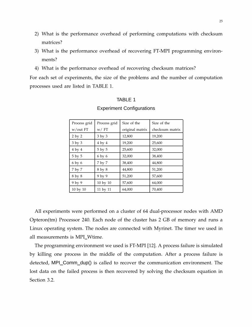
of performing computations with checksum matrices.
Fig. 17 reports the execution time for performing computations on original matrices
and the execution time for performing computations on checksum matrices for different
size of matrices. Fig. 18 reports the overhead (%) for performing computations with
checksum matrices.
Fig. 17 indicates the amount of time increased for performing computations with
28
Overhead for Performing Computation with
Checksum Matrices
0
5
10
15
20
25
30
35
40
45
4 9 16 25 36 49 64 81 100
Number of Processors
Tim
e(S
econd)
Increased
Computation Time
Fig. 17. The overhead (time) for performing computations with encoded matrices
Fig. 18. The overhead (%) for performing computations with encoded matrices
checksum matrices increases slightly as the size of matrices increases. The reason for this
increase is that, when perform computations with checksum matrices, column blocks
of Ac (and row blocks of Br) have to be broadcast to one more process. The dominate
time for parallel matrix matrix multiplication is the time for computation which is the
same for both fault tolerant algorithm and non-fault tolerant algorithm. Therefore, the
amount of time increased for fault tolerant algorithm increases only slightly as the size
of matrices increases. This experimental results agree with our previous theretically
analysis in Section 4.5.3.
Fig. 18 shows that the overhead (%) for performing computations with checksum
matrices decreases as the number of processes increases, which is consistent with our
previous theoretical results (formula (7) in Section 4.5.3).

29
5.3 Overhead for Recovering FT-MPI Environment
The overhead for recovering programming environments depends on the specific pro-
gramming environments. In this section, we evaluate the performance overhead of
recovering FT-MPI environment.
Time for Recovering FT-MPI
0
1
2
3
4
5
6
7
4 9 16 25 36 49 64 81 100
Number of Processors
Tim
e(S
econd)
Time for
Recovering FT-MPI
Fig. 19. The overhead (time) for recovering FT-MPI environment
Fig. 20. The overhead (%) for recovering FT-MPI environment
Fig. 19 reports the time for recovering FT-MPI communication environment with
single process failure. Fig. 20 reports the overhead (%) for recovering FT-MPI com-
munication environment. Fig. 20 indicates that the overhead for recovering FT-MPI is
less than 0.2% which is negligible in practice.
5.4 Overhead for Recovering Application Data
The purpose of this set of experiments is to evaluate the performance overhead of
recovering application data from single process failure.

30
Time for Recovering Data
82
84
86
88
90
92
94
96
98
100
102
4 9 16 25 36 49 64 81 100
Number of Processors
Tim
e(S
econd)
Time for
Recovering Data
Fig. 21. The overhead (time) for recovering application data
Fig. 22. The overhead (%) for recovering application data
Fig. 21 reports the time for recovering the three checksum matrices Ac, Br, and Cf in
the case of single process failure. Fig. 22 reports the overhead (%) recovering the three
checksum matrices Ac, Br, and Cf .
Fig. 21 indicates that, as the number of processes increases, the time for recovering
checksum matrices increases slightly. Fig. 22 indicates that, as the number of processes
increases, the overhead for recovering checksum matrices decreases, which confirmed
our theoretical analysis in Section 4.5.4.
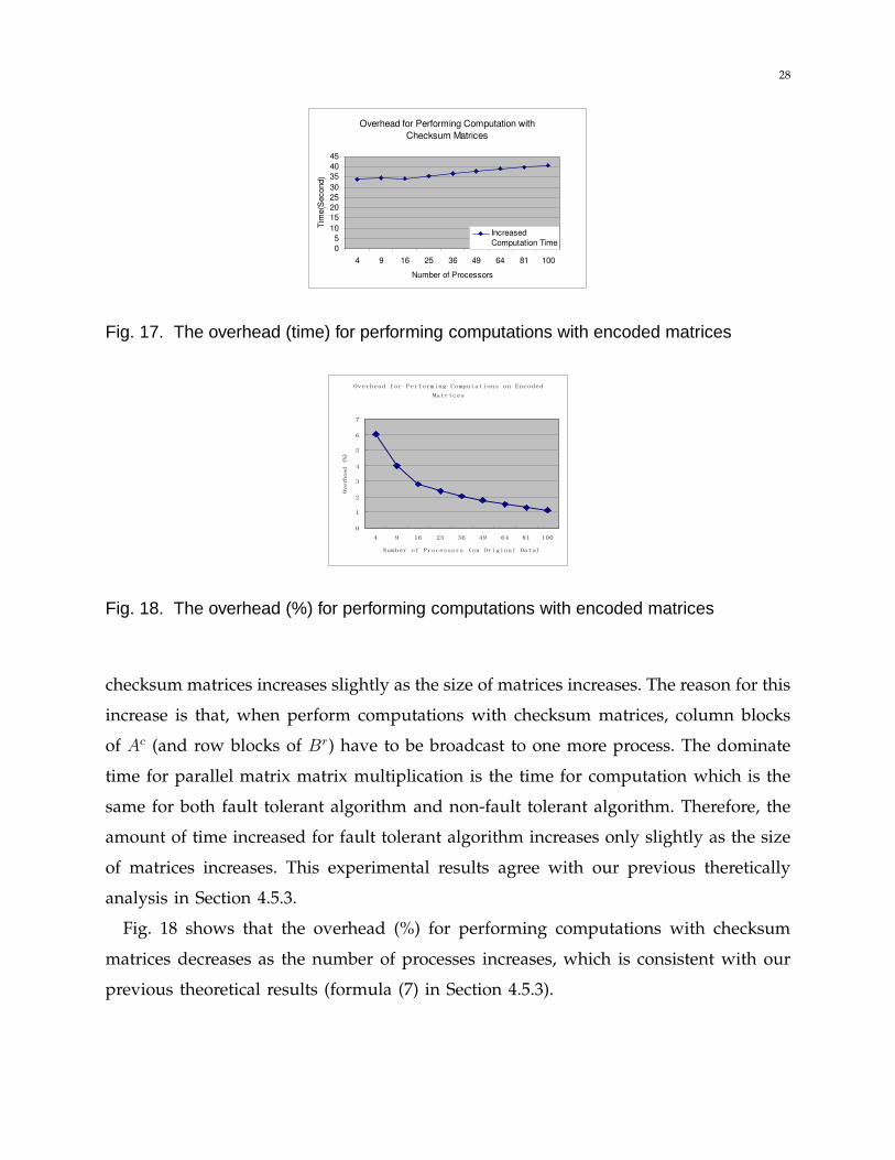
5.5 Total Overhead for Fault Tolerance
When there is no failure occurs, the total overhead equals to the overhead for calculating
encoding at the begining plus the overhead of performing computation with encoded
matrices. If there are failures occur, then the total performance overhead equals the
31
overhead without failures plus the overhead for recovering FT-MPI Environment and
the overhead for recovering the application data.
Fig. 23 reports the execution times of the original matrix-matrix multiplication, the
fault tolerant version matrix-matrix multiplication without failures, and the fault tolerant
version matrix-matrix multiplication with a single process failure. Fig. 24 reports the
total overhead (%) for the proposed algorithm-based checkpoint-free fault tolerance.
Fig. 24 demonstrates that, as the number of processes increases, the total overhead (%)
decreases. This is because, as the number of processors increases, except the overhead
for recovering FT-MPI Environment, all other overhead decreases (as indicated in Sec-
tion 5.1, Section 5.2, and Section 5.3). The overhead for recovering FT-MPI Environment
is less than 0.2% which is not the dominant overhead in the total fault tolerant overhead.
Fig. 23. The total overhead (time) for fault tolerance
Fig. 24. The total overhead (%) for fault tolerance

32
6 DISCUSSION
The idea of tolerating failures by modifying applications to operate on encoded data
comes from the algorithm-based fault tolerance [19]. While Huang and Abraham proved
in [19] that the checksum relationship of the input checksum matrices is preserved in
the final computation results at the end of computation, in this paper, we demonstrated
that for many matrix matrix multiplication algorithms the checksum relationship in the
input checksum matrices does not preserve in the middle of the computation. We further
proved that, for the outer product version matrix matrix multiplcation algorithm, it is
possible to maintain the checksum relationship in the input checksum matrices in the
middle of the computation. Based on our checksum relationship in the middle of the
computation, we demonstrate that fail-stop process failures (which are often tolerated
by checkpointing or message logging) in ScaLAPACK matrix-matrix multiplcation can
be tolerated without checkpointing or message logging.
The algorithm-based checkpoint-free fault tolerance technique presented in this paper
involves solving system of linear equations to recover multiple simultaneous process
failures. Therefore, the practical numerical issues involved in recovering multiple si-
multaneous process failures have to be addressed. Techniques proposed in [7], [8], [11]
addressed part of this issue.
Compared with the typical checkpoint/restart approaches, the algorithm-based checkpoint-
free fault tolerance in this paper can only tolerate partial process failures. It needs
the support from programming environments to detect and locate failures. It requires
the programming environments to be robust enough to survive node failures without
suffering complete system failure. Both the overhead of and the additional effort to
maintain a coded global consistent state of the critical application data in algorithm-
based checkpoint-free fault tolerance is usually highly dependent on the specific char-
acteristic of the application.
Unlike in typical checkpoint/restart approaches which involve periodical checkpoint,
there is no checkpoint involved in this approach. Furthermore, in the algorithm-based
checkpoint-free fault tolerance in this paper, whenever process failures occur, it is only
necessary to recover the lost data on the failed processes. Therefore, for many applica-

33
tions, it is possible for this approach to achieve a much lower fault tolerant overhead
than typical checkpoint/restart approaches. As shown in Section 4 and Section 5, for
matrix matrix multiplication, which is one of the most fundamental operations for
computational science and engineering, as the size N of the matrix increases, the fault
tolerance overhead decreases toward zero with the speed of 1N
.
7 CONCLUSION AND FUTURE WORK
In this paper, we presented a checkpoint-free approach for fault tolerant matrix ma-
trix multiplication in which, instead of taking checkpoint periodically, a coded global
consistent state of the critical application data is maintained in memory by modifying
applications to operate on encoded data. Because no periodical checkpoint or rollback-
recovery is involved in this approach, process failures can often be tolerated with a
surprisingly low overhead. We showed the practicality of this technique by applying
it to the ScaLAPACK matrix-matrix multiplication kernel which is one of the most
important kernels for ScaLAPACK library to achieve high performance and scalability.
Experimental results demonstrated that the proposed checkpoint-free approach is able
to survive process failures with a very low performance overhead.
There are many directions in which this work could be extended. The first direction is
to extend this checkpoint-free approach to more applications. The second direction is to
extend this technique to tolerate multiple simutaneous failures. Furthermore, it is also
interesting to extend the approach to tolerate failures occured during synchronization
and recovery.
ACKNOWLEDGMENT
This research was supported in part by the Los Alamos National Laboratory under
Contract No. 03891-001-99 49 and the Applied Mathematical Sciences Research Program
of the Office of Mathematical, Information, and Computational Sciences, U.S. Depart-
ment of Energy under contract DE-AC05-00OR22725 with UT-Battelle, LLC. The authors
would like to thank the anonymous reviewers for their valuable comments.

34
REFERENCES
[1] J. Anfinson and F. T. Luk A Linear Algebraic Model of Algorithm-Based Fault Tolerance. IEEE Transactions on
Computers, v.37 n.12, p.1599-1604, December 1988.
[2] P. Banerjee, J. T. Rahmeh, C. B. Stunkel, V. S. S. Nair, K. Roy, V. Balasubramanian, and J. A. Abraham Algorithm-
based fault tolerance on a hypercube multiprocessor. IEEE Transactions on Computers, vol. C-39:1132–1145, 1990.
[3] V. Balasubramanian and P. Banerjee Compiler-Assisted Synthesis of Algorithm-Based Checkingin Multiproces-
sors. IEEE Transactions on Computers, vol. C-39:436-446, 1990.
[4] L. S. Blackford, J. Choi, A. Cleary, A. Petitet, R. C. Whaley, J. Demmel, I. Dhillon, K. Stanley, J. Dongarra,
S. Hammarling, G. Henry, and D. Walker. ScaLAPACK: a portable linear algebra library for distributed memory
computers - design issues and performance. In Supercomputing ’96: Proceedings of the 1996 ACM/IEEE conference
on Supercomputing (CDROM), page 5, 1996.
[5] D. L. Boley, R. P. Brent, G. H. Golub, and F. T. Luk. Algorithmic fault tolerance using the lanczos method. SIAM
Journal on Matrix Analysis and Applications, 13:312–332, 1992.
[6] L. E. Cannon. A cellular computer to implement the kalman filter algorithm. Ph.D. thesis, Montana State University,
Bozeman, MT, USA, 1969.
[7] Z. Chen and J. Dongarra. Numerically stable real number codes based on random matrices. In Proceeding of the
5th International Conference on Computational Science (ICCS2005), Atlanta, Georgia, USA, May 22-25, 2005. LNCS
3514, Springer-Verlag.
[8] Z. Chen and J. Dongarra. Condition Numbers of Gaussian Random Matrices. SIAM Journal on Matrix Analysis
and Applications, Volume 27, Number 3, Page 603-620, 2005.
[9] Z. Chen, G. E. Fagg, E. Gabriel, J. Langou, T. Angskun, G. Bosilca, and J. Dongarra. Fault tolerant high
performance computing by a coding approach. In Proceedings of the ACM SIGPLAN Symposium on Principles and
Practice of Parallel Programming, PPOPP 2005, June 14-17, 2005, Chicago, IL, USA. ACM, 2005.
[10] Z. Chen, G. E. Fagg, E. Gabriel, J. Langou, T. Angskun, G. Bosilca, and J. Dongarra. Building Fault Survivable
MPI Programs with FT-MPI Using Diskless Checkpointing. In University of Tennessee Computer Science Department
Technical Report. Technical Report UT-CS-04-540, 2004.
[11] Z. Chen. Scalable techniques for fault tolerant high performance computing. Ph.D. thesis, University of Tennessee,
Knoxville, TN, USA, 2006.
[12] G. E. Fagg, E. Gabriel, G. Bosilca, T. Angskun, Z. Chen, J. Pjesivac-Grbovic, K. London, and J. J. Dongarra.
Extending the MPI specification for process fault tolerance on high performance computing systems. In
Proceedings of the International Supercomputer Conference, Heidelberg, Germany, 2004.
[13] G. E. Fagg, E. Gabriel, Z. Chen, , T. Angskun, G. Bosilca, J. Pjesivac-Grbovic, and J. J. Dongarra. Process fault-
tolerance: Semantics, design and applications for high performance computing. Submitted to International Journal
of High Performance Computing Applications, 2004.
[14] I. Foster and C. Kesselman. The Grid: Blueprint for a New Computing Infrastructure. Morgan Kauffman, San
Francisco, 1999.
[15] I. Foster and C. Kesselman. The GLOBUS toolkit. The grid: blueprint for a new computing infrastructure, pages
259–278, 1999.
[16] G. C. Fox, M. Johnson, G. Lyzenga, S. W. Otto, J. Salmon, and D. Walker. Solving Problems on Concurrent
Processors: Volum 1. Prentice-Hall, Englewood Cliffs, NJ, 1988.

35
[17] E. Gabriel, G. E. Fagg, G. Bosilca, T. Angskun, J. Dongarra, J. M. Squyres, V. Sahay, P. Kambadur, B. Barrett,
A. Lumsdaine, R. H. Castain, D. J. Daniel, R. L. Graham, and T. S. Woodall. Open MPI: Goals, concept, and
design of a next generation MPI implementation. In PVM/MPI, pages 97–104, 2004.
[18] G. H. Golub and C. F. Van Loan. Matrix Computations. The John Hopkins University Press, , 1989.
[19] K.-H. Huang and J. A. Abraham. Algorithm-based fault tolerance for matrix operations. IEEE Transactions on
Computers, vol. C-33:518–528, 1984.
[20] Y. Kim. Fault Tolerant Matrix Operations for Parallel and Distributed Systems. Ph.D. dissertation, University of
Tennessee, Knoxville, June
[21] F. T. Luk and H. Park An analysis of algorithm-based fault tolerance techniques. SPIE Adv. Alg. and Arch. for
Signal Proc., vol. 696, 1986, pp. 222-228.
[22] J. S. Plank, Y. Kim, and J. Dongarra. Fault Tolerant Matrix Operations for Networks of Workstations Using
Diskless Checkpointing. IEEE Journal of Parallel and Distributed Computing, 43, 125-138 (1997).
[23] J. S. Plank, K. Li, and M. A. Puening. Diskless checkpointing. IEEE Trans. Parallel Distrib. Syst., 9(10):972–986,
1998.
[24] J. S. Plank. A tutorial on Reed-Solomon coding for fault-tolerance in RAID-like systems. Software – Practice &
Experience, 27(9):995–1012, September 1997.
[25] P. Sanders and J. F. Sibeyn. A bandwidth latency tradeoff for broadcast and reduction. Inf. Process. Lett.,
86(1):33–38, 2003.
[26] M. Snir, S. Otto, S. Huss-Lederman, D. W. Walker, and J. Dongarra. MPI: The Complete Reference. Volume 1, The
MIT Press, 2nd edition, 1998.
[27] V. S. Sunderam. PVM: a framework for parallel distributed computing. Concurrency: Pract. Exper., 2(4):315–339,
1990.
[28] C. Wang, F. Mueller, C. Engelmann, and S. Scot. Job Pause Service under LAM/MPI+BLCR for Transparent
Fault Tolerance. In Proceedings of the 21st IEEE International Parallel and Distributed Processing Symposium, March,
2007, Long Beach, CA, USA.
Recommended


![IEEE TRANSACTIONS ON COMPUTERS, VOL. 62, NO. 11, · PDF fileTo tolerate more failures than RAID, many storage systems employ Reed-Solomon codes for fault-tolerance [9], [10]. Reed-](https://img.pdfslide.net/doc/110x75/5ab7ceb97f8b9ac10d8c313d/ieee-transactions-on-computers-vol-62-no-11-tolerate-more-failures-than.jpg)