1
CE 530 Molecular Simulation
Lecture 18
Free-energy calculations
David A. Kofke
Department of Chemical Engineering
SUNY Buffalo
2
Free-Energy Calculations
Uses of free energy• Phase equilibria
• Reaction equilibria
• Solvation
• Stability
• Kinetics
Calculation methods• Free-energy perturbation
• Thermodynamic integration
• Parameter-hopping
• Histogram interpolation
3
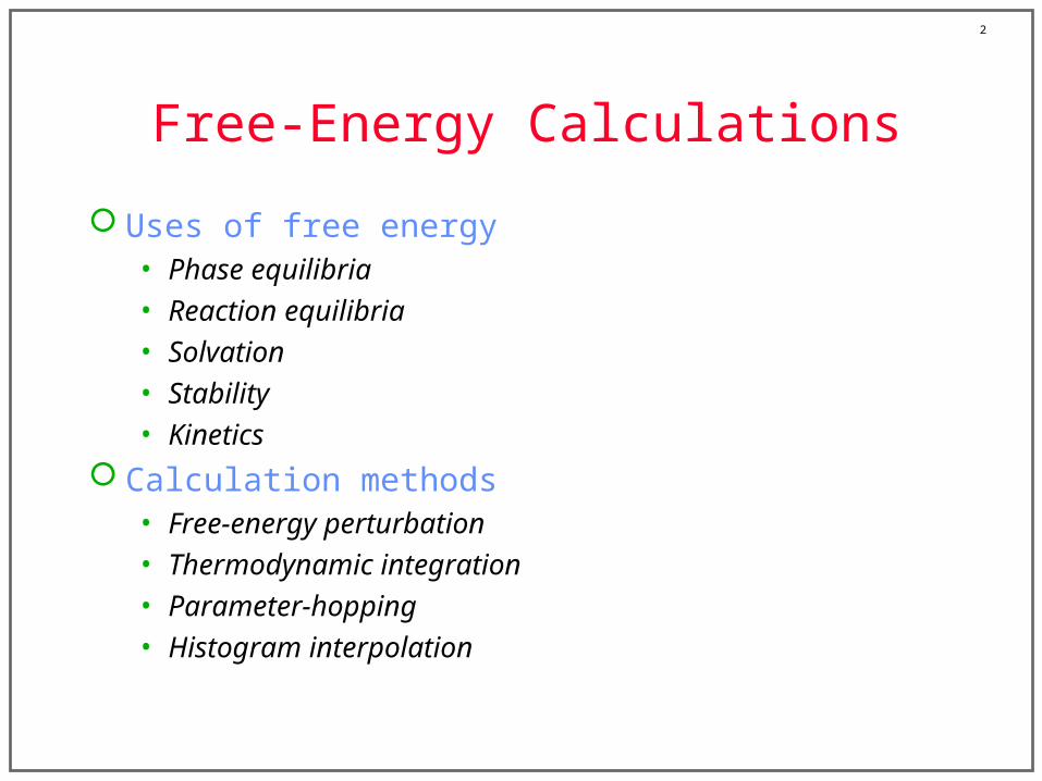
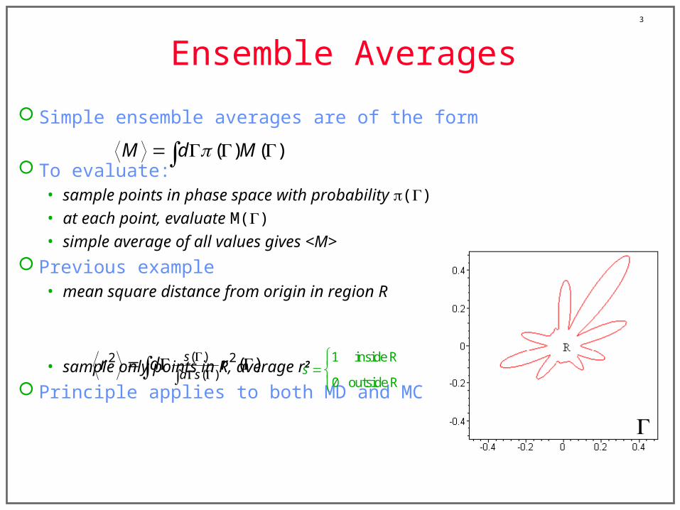
Ensemble Averages
Simple ensemble averages are of the form
To evaluate:• sample points in phase space with probability ()
• at each point, evaluate M()
• simple average of all values gives <M>
Previous example• mean square distance from origin in region R
• sample only points in R, average r2
Principle applies to both MD and MC
( ) ( )M d M
( )2 2( )
( )s
d sr d r
1 inside R
0 outside Rs
4
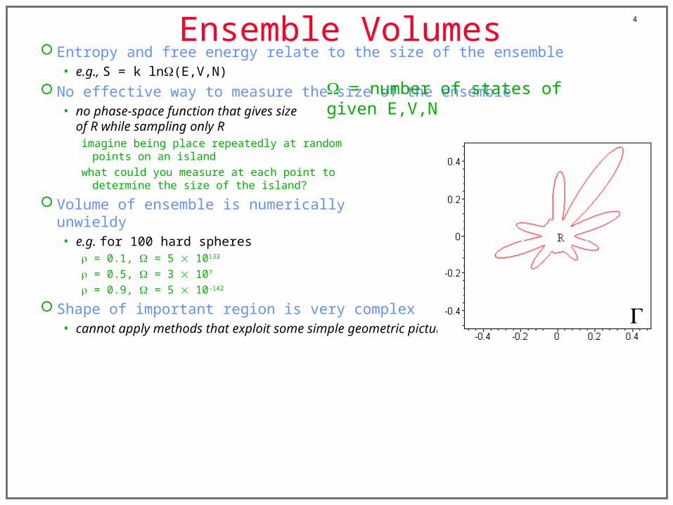
Ensemble Volumes Entropy and free energy relate to the size of the ensemble
• e.g., S = k ln(E,V,N)
No effective way to measure the size of the ensemble• no phase-space function that gives size
of R while sampling only Rimagine being place repeatedly at random
points on an island
what could you measure at each point todetermine the size of the island?
Volume of ensemble is numericallyunwieldy• e.g. for 100 hard spheres
= 0.1, = 5 10133
= 0.5, = 3 107
= 0.9, = 5 10-142
Shape of important region is very complex• cannot apply methods that exploit some simple geometric picture
= number of states of given E,V,N
5
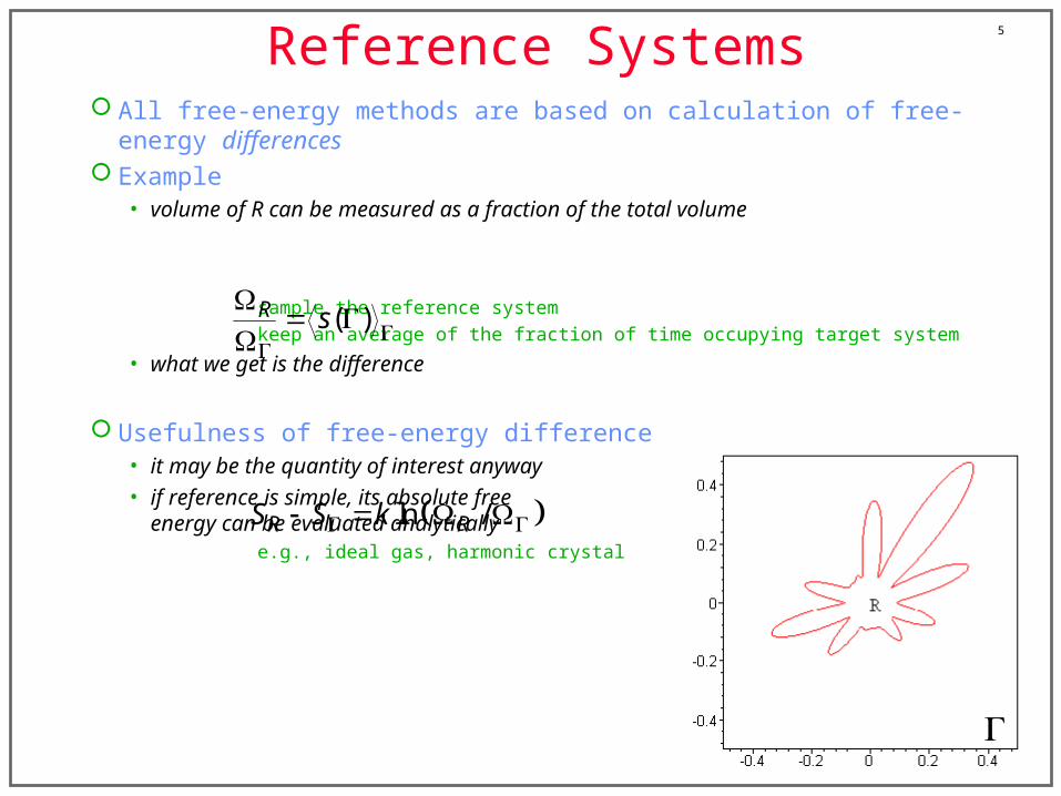
Reference Systems All free-energy methods are based on calculation of free-energy differences Example
• volume of R can be measured as a fraction of the total volume
sample the reference system
keep an average of the fraction of time occupying target system
• what we get is the difference
Usefulness of free-energy difference• it may be the quantity of interest anyway
• if reference is simple, its absolute free energy can be evaluated analytically
e.g., ideal gas, harmonic crystal
( )R s
ln /R RS S k

6
Chemical potential is an entropy difference
For hard spheres, the energy is zero or infinity• any change in N that does not cause overlap will be change at constant U
To get entropy difference• simulate a system of N+1 spheres, one non-interacting “ghost”
• occasionally see if the ghost sphere overlaps another
• record the fraction of the time it does not overlap
Here is an applet demonstrating this calculation
,
/( , , 1) ( , , )
U V
S kS U V N S U V N
N
3
/ 1non-overlap3 3
S k NV
NN
V Ve e f
N N
N+1
N
×
×
Hard Sphere Chemical Potential
7
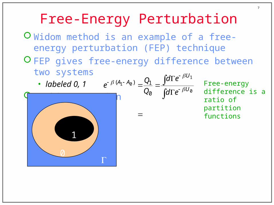
Free-Energy PerturbationWidom method is an example of a free-energy perturbation
(FEP) technique FEP gives free-energy difference between two systems
• labeled 0, 1
Working equation
1 0 0
0
1 0
1
1 0
0
0
1
( )
( )0
( ) 1
0
( )
0
)
UA A
U U U
U
U U
U U
U
d e e
d eQe
Q
d e
d e
e
e
d
0
1
Free-energy difference is a ratio of partition functions

8
Free-Energy PerturbationWidom method is an example of a free-energy perturbation
(FEP) technique FEP gives free-energy difference between two systems
• labeled 0, 1
Working equation
1 0
1 0
1
1 0
1
0
0
0
0
( )0
( )
( ) 1
0
( )
0
)U U
U U
UA A
U
U
U
U U
d eQe
Q d e
d e e
d e
d e
e
0
1
Add and subtract reference-system energy

9
Free-Energy PerturbationWidom method is an example of a free-energy perturbation
(FEP) technique FEP gives free-energy difference between two systems
• labeled 0, 1
Working equation1
1 0
0
1 0 0
0
1
1
0
0
( ) 1
0
( )
( )0
( )
0
)
UA A
U
U U U
U
U
U U
U
d eQe
Q d e
d e e
e
e
d
d e
0
1 Identify reference-system probability distribution

10
Free-Energy PerturbationWidom method is an example of a free-energy perturbation (FEP)
technique FEP gives free-energy difference between two systems
• labeled 0, 1
Working equation
Sample the region important to 0 system, measure properties of 1 system
1
1 0
0
1 0 0
0
1 0
1 0
( ) 1
0
( )
( )0
( )
0
)
UA A
U
U U U
U
U U
U U
d eQe
Q d e
d e e
d e
d e
e
0
1Write as reference-system ensemble average

11
Chemical potential
For chemical potential, U1 - U0 is the energy of turning on the ghost particle• call this ut, the “test-particle” energy
• test-particle position may be selected at random in simulation volume
• for hard spheres, e-ut is 0 for overlap, 1 otherwisethen (as before) average is the fraction of configurations with no overlap
This is known as Widom’s insertion method
1 0
3
( )
0t
A A
uVN
e e
e
12
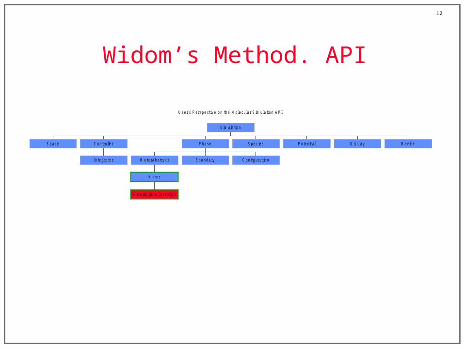
Widom’s Method. API
U ser 's P erspe ctiv e o n the M o lecu la r S im u la tion A P I
S pa ce
In te gra to r
C on tro lle r
M ete rW ido m Inse rtion
M ete r
M e te rA b s tra ct B ou nda ry C on fig u ra tion
P ha se S p ec ies P o te n tia l D isp lay D ev ice
S im u la tion
13
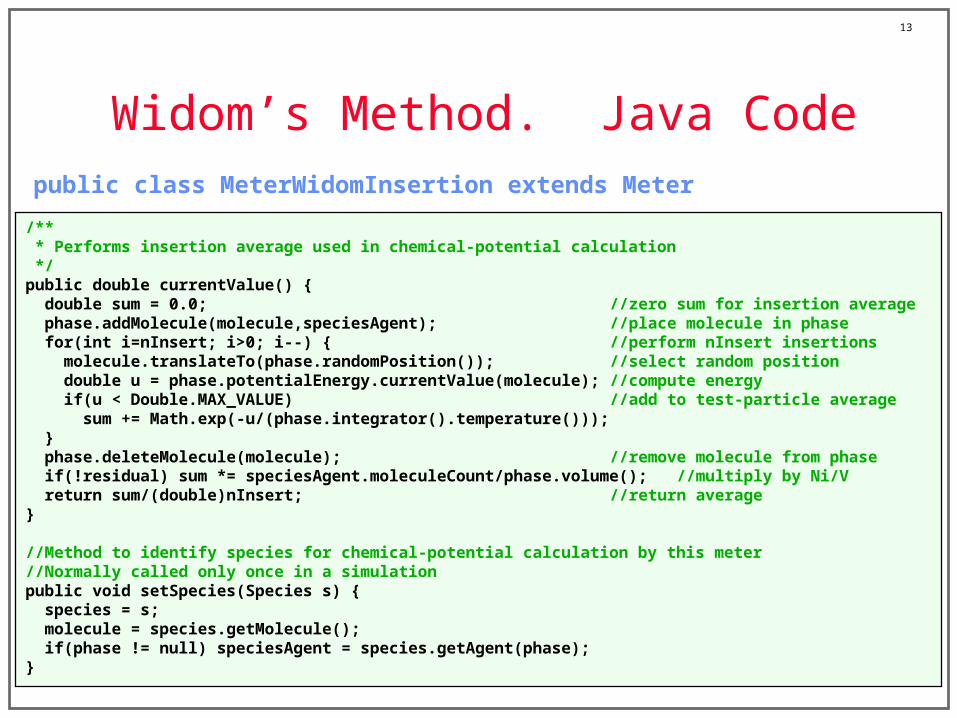
Widom’s Method. Java Codepublic class MeterWidomInsertion extends Meter
/** * Performs insertion average used in chemical-potential calculation */public double currentValue() { double sum = 0.0; //zero sum for insertion average phase.addMolecule(molecule,speciesAgent); //place molecule in phase for(int i=nInsert; i>0; i--) { //perform nInsert insertions molecule.translateTo(phase.randomPosition()); //select random position double u = phase.potentialEnergy.currentValue(molecule); //compute energy if(u < Double.MAX_VALUE) //add to test-particle average sum += Math.exp(-u/(phase.integrator().temperature())); } phase.deleteMolecule(molecule); //remove molecule from phase if(!residual) sum *= speciesAgent.moleculeCount/phase.volume(); //multiply by Ni/V return sum/(double)nInsert; //return average}
//Method to identify species for chemical-potential calculation by this meter//Normally called only once in a simulationpublic void setSpecies(Species s) { species = s; molecule = species.getMolecule(); if(phase != null) speciesAgent = species.getAgent(phase);}
14
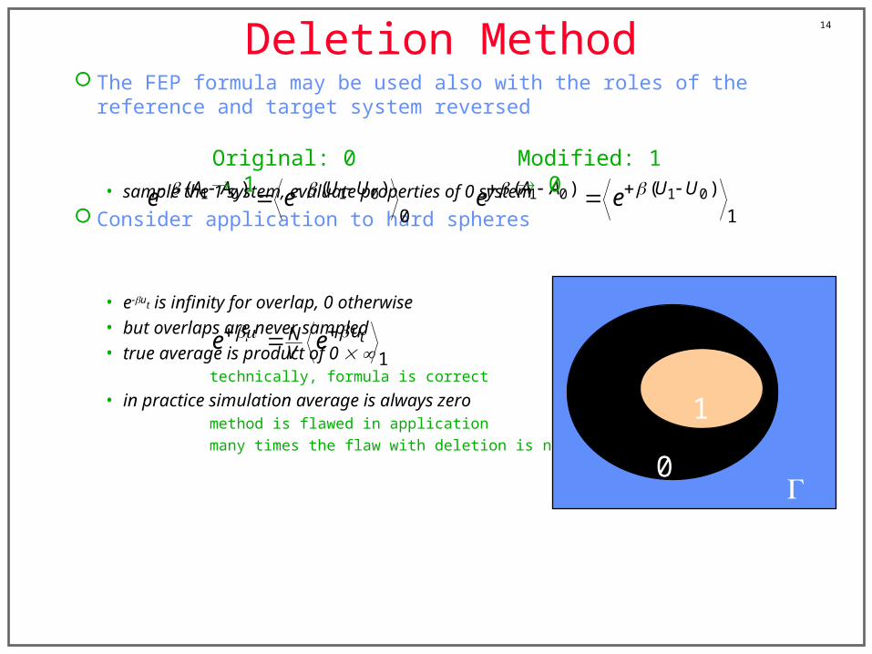
Deletion Method The FEP formula may be used also with the roles of the reference and target system
reversed
• sample the 1 system, evaluate properties of 0 system
Consider application to hard spheres
• e-ut is infinity for overlap, 0 otherwise
• but overlaps are never sampled
• true average is product of 0 technically, formula is correct
• in practice simulation average is always zeromethod is flawed in application
many times the flaw with deletion is not as obvious as this
1 0 1 0( ) ( )
0
A A U Ue e 1 0 1 0( ) ( )
1
A A U Ue e
0
1
Original: 0 1 Modified: 1 0
1tuN
Ve e
15
Other Types of PerturbationMany types of free-energy differences can be computed Thermodynamic state
• temperature, density, mixture composition
Hamiltonian• for a single molecule or for entire system
• e.g., evaluate free energy difference for hard spheres with and without electrostatic dipole moment
Configuration• distance/orientation between two solutes
• e.g, protein and ligand
Order parameter identifying phases• order parameter is a quantity that can be used to identify the thermodynamic phase a
system is in
• e.g, crystal structure, orientational order, magnetization
16
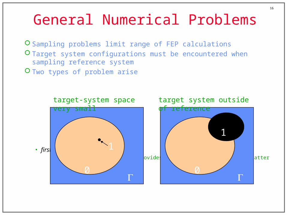
General Numerical Problems
Sampling problems limit range of FEP calculations Target system configurations must be encountered when sampling reference
system Two types of problem arise
• first situation is more common although deletion FEP provides an avoidable example of the latter
0
1
target-system space very small
0
1
target system outside of reference
17
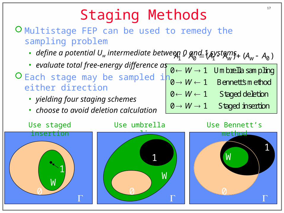
Staging MethodsMultistage FEP can be used to remedy the sampling problem
• define a potential Uw intermediate between 0 and 1 systems
• evaluate total free-energy difference as
Each stage may be sampled in either direction• yielding four staging schemes
• choose to avoid deletion calculation
1 0 1 0( ) ( )w wA A A A A A
0
1
W
0 1 Umbrella sampling
0 1 Bennett's method
0 1 Staged deletion
0 1 Staged insertion
W
W
W
W
Use staged insertion Use umbrella sampling
0
1
W
0
1
Use Bennett’s method
W
18
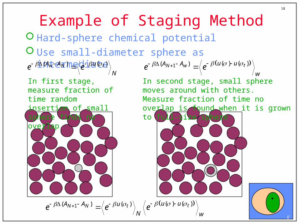
Example of Staging Method Hard-sphere chemical potential Use small-diameter sphere as intermediate
( ) ( )w N tA A u
Ne e
In first stage, measure fraction of time random insertion of small sphere finds no overlap
1 ( ) ( )( ) tN w u uA A
we e
In second stage, small sphere moves around with others. Measure fraction of time no overlap is found when it is grown to full-size sphere
1 ( ) ( )( ) ( ) tN N t u uA A u
N we e e
19
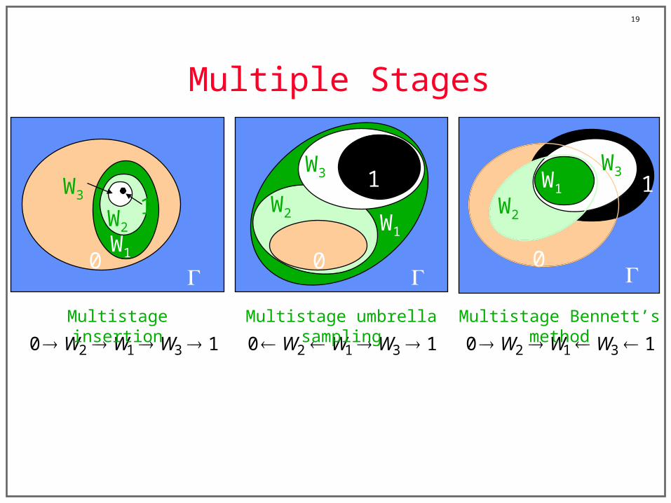
Multiple Stages
0
1
W1
W2
W3
0
1
W1
W2
W3
2 1 30 1W W W
0
1W1
W3
W2
2 1 30 1W W W 2 1 30 1W W W Multistage insertion Multistage umbrella sampling Multistage Bennett’s method
20
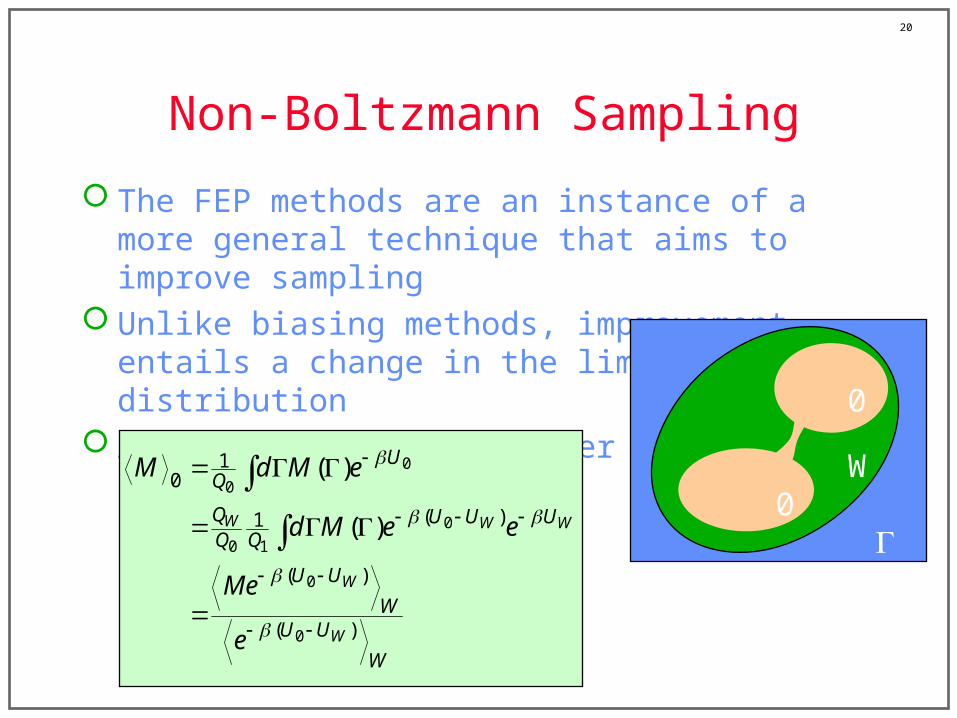
Non-Boltzmann Sampling
The FEP methods are an instance of a more general technique that aims to improve sampling
Unlike biasing methods, improvement entails a change in the limiting distribution
Apply a formula to recover the correct average
0
0
0
0 1
0
0
10
( )1
( )
( )
( )
( )W W W
W
W
UQ
Q U U UQ Q
U U
WU U
W
M d M e
d M e e
Me
e
W
0
0

21
Thermodynamic Integration 1.
Thermodynamics gives formulas for variation of free energy with state
These can be integrated to obtain a free-energy difference• derivatives can be measured as normal ensemble averages
• this is usually how free energies are “measured” experimentally
d A Ud PdV dN
,, T NV N
A AU P
V
2
1
2 1( ) ( ) ( )V
V
A V A V P V dV
22
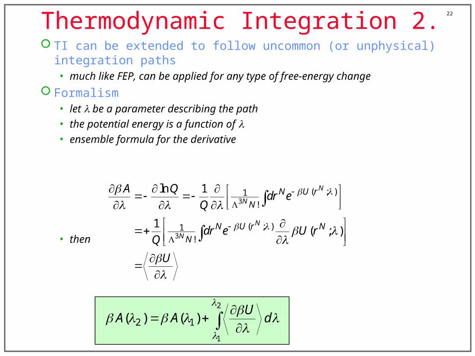
Thermodynamic Integration 2. TI can be extended to follow uncommon (or unphysical) integration paths
• much like FEP, can be applied for any type of free-energy change
Formalism• let be a parameter describing the path
• the potential energy is a function of • ensemble formula for the derivative
• then
3
3
( ; )1!
( ; )1!
ln 1
1( ; )
N
N
N
N
N U r
N
N U r N
N
A Qdr e
Q
dr e U rQ
U
2
1
2 1( ) ( )U
A A d
23
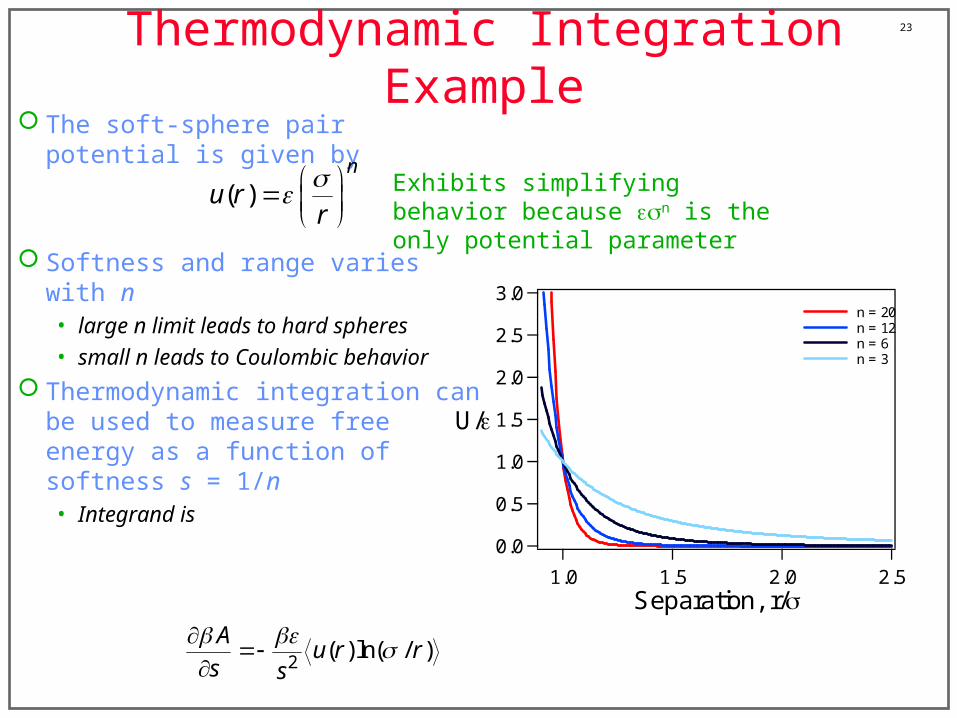
Thermodynamic Integration Example The soft-sphere pair potential is
given by
Softness and range varies with n• large n limit leads to hard spheres
• small n leads to Coulombic behavior
Thermodynamic integration can be used to measure free energy as a function of softness s = 1/n• Integrand is
( )n
u rr
Exhibits simplifying behavior because n is the only potential parameter
2( ) ln( / )
Au r r
s s
3.0
2.5
2.0
1.5
1.0
0.5
0.0
U/
2.52.01.51.0Separation, r/
n = 20 n = 12 n = 6 n = 3

24
Parameter Hopping. Theory View free-energy parameter as another dimension in phase
space
Partition function
Monte Carlo trials include changes in Probability that system has 0 or = 1
( , , )N NE E p r
0
1
0 1
( , , )
( , , ) ( , , )
0 1
N N
N N N N
N N E
E EN N N N
Q d d e
d d e d d e
Q Q
p r
p r p r
p r
p r p r
00
0 1 0 1
11
0 1 0 1
( , , )10
( , , )11
( )
( )
N N
N N
QEN NQ Q Q Q
QEN NQ Q Q Q
d d e
d d e
p r
p r
p r
p r
25
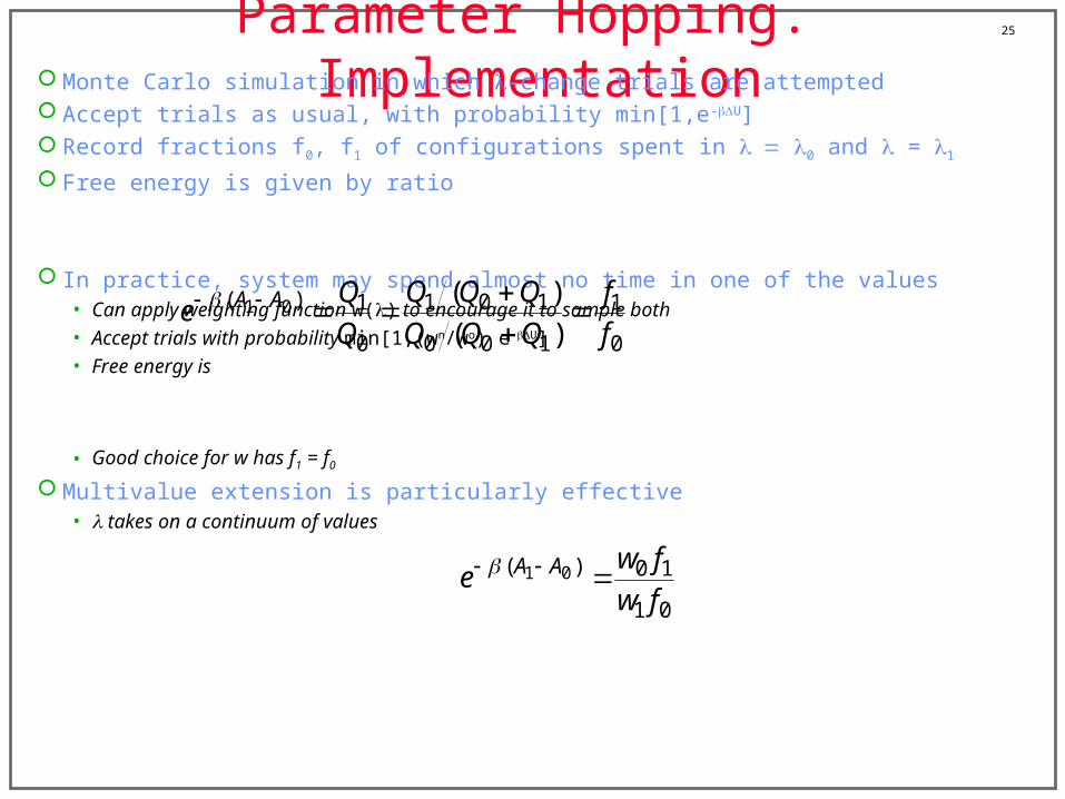
Parameter Hopping. ImplementationMonte Carlo simulation in which -change trials are attempted Accept trials as usual, with probability min[1,e-U] Record fractions f0, f1 of configurations spent in 0 and = 1
Free energy is given by ratio
In practice, system may spend almost no time in one of the values• Can apply weighting function w() to encourage it to sample both
• Accept trials with probability min[1,(wn/wo) e-U]
• Free energy is
• Good choice for w has f1 = f0
Multivalue extension is particularly effective• takes on a continuum of values
1 0( ) 1 0 11 1
0 0 0 1 0
( )
( )A A Q Q QQ f
eQ Q Q Q f
1 0( ) 0 1
1 0
A A w fe
w f
26
Summary Free energy calculations are needed to model the most interesting physical
behaviors• All useful methods are based on computing free-energy difference
Four general approaches• Free-energy perturbation
• Thermodynamic integration
• Parameter hopping
• Distribution-function methods
FEP is asymmetric• Deletion method is awful
Four approaches to basic multistaging• Umbrella sampling, Bennett’s method, staged insertion/deletion
Non-Boltzmann methods improve sampling
Recommended