The Sandwich Variance Estimator: EÆciency Properties
and Coverage Probability of Con�dence Intervals
G�oran Kauermann � Raymond J. Carroll y
December 16, 1999
Abstract
The sandwich estimator, often known as the robust covariance matrix estimator or
the empirical covariance matrix estimator, has achieved increasing use with the growing
popularity of generalized estimating equations. Its virtue is that it provides consistent
estimates of the covariance matrix for parameter estimates even when the �tted para-
metric model fails to hold, or is not even speci�ed. Surprisingly though, there has been
little discussion of the properties of the sandwich method other than consistency. We
investigate the sandwich estimator in quasilikelihood models asymptotically, and in
the linear case analytically. We show that when the quasilikelihood model is correct,
the sandwich estimate is often far more variable than the usual parametric variance
estimate. The increased variance is a �xed feature of the method, and the price one
pays to obtain consistency even when the parametric model fails. We show that the
additional variability directly a�ects the coverage probability of con�dence intervals
constructed from sandwich variance estimates. In fact the use of sandwich estimates
combined with t-distribution quantiles gives con�dence intervals with coverage proba-
bility falling below the nominal value. We propose a simple adjustment to compensate
this defect, where the adjustment explicitly considers the variance of the sandwich
estimate.
Keywords: Coverage probability; Generalized estimating equations; Generalized linearmodels; Heteroscedasticity; Linear regression; Quasilikelihood; Robust covariance estima-tor; Sandwich estimator.
Short Title: The Sandwich Estimator
�Institute of Statistics; Ludwig-Maximilians-University Munich; Akademiestr. 1; 80796 Munich, GermanyyDepartment of Statistics, Texas A & M University, College Station, TX 77843-3143, USA. Research
was supported by a grant from National Cancer Institute (CA{57030), and by the Texas A&M Center forEnvironmental and Rural Health via a grant from the National Institute of Environmental Health Sciences(P30-ESO9106).
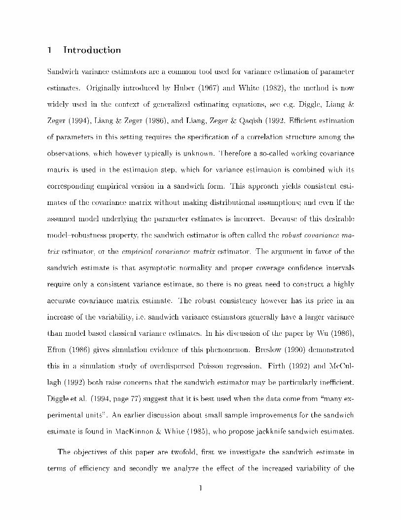
1 Introduction
Sandwich variance estimators are a common tool used for variance estimation of parameter
estimates. Originally introduced by Huber (1967) and White (1982), the method is now
widely used in the context of generalized estimating equations, see e.g. Diggle, Liang &
Zeger (1994), Liang & Zeger (1986), and Liang, Zeger & Qaqish (1992. EÆcient estimation
of parameters in this setting requires the speci�cation of a correlation structure among the
observations, which however typically is unknown. Therefore a so-called working covariance
matrix is used in the estimation step, which for variance estimation is combined with its
corresponding empirical version in a sandwich form. This approach yields consistent esti-
mates of the covariance matrix without making distributional assumptions; and even if the
assumed model underlying the parameter estimates is incorrect. Because of this desirable
model{robustness property, the sandwich estimator is often called the robust covariance ma-
trix estimator, or the empirical covariance matrix estimator. The argument in favor of the
sandwich estimate is that asymptotic normality and proper coverage con�dence intervals
require only a consistent variance estimate, so there is no great need to construct a highly
accurate covariance matrix estimate. The robust consistency however has its price in an
increase of the variability, i.e. sandwich variance estimators generally have a larger variance
than model based classical variance estimates. In his discussion of the paper by Wu (1986),
Efron (1986) gives simulation evidence of this phenomenon. Breslow (1990) demonstrated
this in a simulation study of overdispersed Poisson regression. Firth (1992) and McCul-
lagh (1992) both raise concerns that the sandwich estimator may be particularly ineÆcient.
Diggle et al. (1994, page 77) suggest that it is best used when the data come from \many ex-
perimental units". An earlier discussion about small sample improvements for the sandwich
estimate is found in MacKinnon & White (1985), who propose jackknife sandwich estimates.
The objectives of this paper are twofold, �rst we investigate the sandwich estimate in
terms of eÆciency and secondly we analyze the e�ect of the increased variability of the
1

sandwich estimate on the coverage probability of con�dence intervals. For the �rst point we
derive asymptotic as well as fairly precise small sample properties, neither of which appear to
have been quanti�ed before. For example, the sandwich method in simple linear regression
when estimating the slope has an asymptotic ineÆciency equal to the inverse of the sample
kurtosis of the design values. This ineÆciency still holds in generalized linear models. For
example, in simple linear logistic regression, at the null value where there is no e�ect due
to the predictor, the sandwich method's asymptotic relative eÆciency is again the inverse
of the kurtosis of the predictors. In Poisson regression, the sandwich method has even less
eÆciency.
The problem of coverage probability of con�dence intervals built from sandwich variance
estimates is discussed in the second part of the paper. Simulation studies given by Wu
(1986) and Breslow (1990) report somewhat elevated levels of Wald{type tests based on the
sandwich estimator. Rothenberg (1988) derives an adjusted distribution function for the
t statistic calculated from sandwich variance estimates. We give a theoretical justi�cation
for the empirical fact that con�dence intervals calculated from sandwich variance estimates
and t-distribution quantiles are generally too small, i.e. the coverage probability falls below
the nominal value. We apply an Edgeworth expansion and concentrate on the coverage
probability of con�dence intervals. We show that undercoverage is mainly determined by
the variance of the variance estimate. To correct this de�cit we present a simple adjustment
which depends on normal distribution quantiles and the variance of the sandwich variance
estimate.
The paper is organized as follows. In Section 2 we compare the sandwich estimator
with the usual parametric regression estimator in the homoscedastic linear regression model.
Section 3 gives a discussion of the sandwich estimate for quasilikelihood and generalized
estimating equations (GEE). Some simulations are presented in Section 4 where we suggest
a simple adjustment which improves coverage probability. Section 5 contains concluding
2

remarks. Proofs and general statements are given in the appendix.
2 Linear Regression
2.1 The Sandwich Estimator
Consider the simple linear regression model yi = xTi � + �i, i = 1; : : : ; n where xTi are 1� p
dimensional vectors of covariates and �i � N(0; �2). Let b� = (XTX)�1XTY be the ordinary
least squares estimator of � where YT = (y1; : : : yn) and XT = (x1; : : :xn). Assume now
that we are interested in inference about the linear combination zT b�, where zT is a 1 � p
dimensional contrast vector of unit length, i.e. zTz = 1. The variance of zT b� is given by
var(zT b�) = �2zT(XTX)�1z which can be estimated by the classical model based variance
estimator Vmodel = �̂2zT(XTX)�1z where �̂2 =Pn
i=1 b�2i =(n� p) with b�i = Yi � xTi b� as �tted
residuals. A major assumption implicitly used in the calculation of Vmodel is that the errors �i
are homoscedastic. If this assumption is violated Vmodel does not provide a consistent variance
estimate. In contrast even if the errors are not homoscedastic the sandwich variance estimate
Vsand = zT(XTX)�1(Xi
xixTi b�2i )(XTX)�1z =
nXi=1
a2i b�2i : (1)
consistently estimates var(zT b�), where ai = zT(XTX)�1xi. In linear regression, (1) is often
multiplied by n=(n� p) (Hinkley, 1977) to reduce the bias.
2.2 Properties of Sandwich Estimator
Let hii be the i-th digonal element of the hat matrix H = X(XTX)�1XT = (hij). Under
homoscedasticity, E(b�2i ) = �2(1� hii). It then follows that
E(Vsand) = �2zT(XTX)�1z(1� bn); (2)
where bn =Pn
i=1 hiia2i =Pn
i=1 a2i � max1�i�n hii. Since bn � 0 one obtains that in general the
sandwich estimator is biased downward. The bias thereby depends on the design of xi and
it can be substantial when there are leverage points. To demonstrate this let the �rst point
3

be a leverage point such that h11 = max1�i�n hii and set z = x1=nx1(X
TX)�1xT1o1=2
. Then
the bias of the sandwich estimator satis�es
maxzT(XTX)�1z=1
jbias(Vsand)j � �2 max1�i�n
h2ii:
Thus, if there is a large leverage point, the usual sandwich estimator can be expected to
have poor bias behavior relative to the classical formula.
Bias problems can be avoided by replacing b�i in (1) by e�i = b�i=(1� hii)1=2. The resulting
estimator is refered to as unbiased sandwich variance estimator in the following denoted by
Vsand;u (see also Wu, 1986, equation 2.6). It is easily seen that E(Vsand;u) = var(zb�). Sincevar(e�2i ) = 2�4 and cov(e�2i ; e�2j) = 2eh2ij�4 for i 6= j, where ehij = hij=f(1 � hii)(1 � hjj)g1=2, itfollows that
var(Vsand;u) =nX
i=1
a4ivar(e�2) +Xi 6=j
a2i a2jcov(e�2i ; e�2j) = 2�4
nXi=1
a4i + 2�4Xi6=j
a2i a2jeh2ij: (3)
We now compare the variance (3) to the variance of the model based variance estimator
Vmodel which equals var(Vmodel) � 2�4fzT(XTX)�1zg2=n = 2�4(Pa2a)
2=n.
Theorem 1: Under the homoscedastic linear model the eÆciency of the unbiased sandwich
estimate Vsand;u compared to the classical variance estimate Vmodel for zT b� satisfy:
var(Vsand)
var(Vmodel)� fn�1
nXi=1
a4i gfn�1nX
i=1
a2i g�2 � 1: (4)
If in addition max(hii) = o(n�1=2), then the middle term in (4) gives the asymptotic relative
eÆciency.
The proof follows directly from the Cauchy Schwarz inequality. Theorem 1 states that
the sandwich estimate is less eÆcient when the model is correct, i.e. when the errors are
homescedastic. The loss of eÆciency is thereby inversely proportional to the kurtosis of the
design points as the following two examples show.
4

Example 1 (the intercept): Suppose the �rst column of X is a vector of ones, the other
columns have means of zero, and zT = (1; 0; : : : ; 0). We then have ai = n�1 and the
asymptotic relative eÆciency in (4) is 1.
Example 2 (the slope in simple linear regression): Assume xTi = (1; ui) wherePui = 0.
Suppose z = (0; 1) so that b�1 = zb� is the slope estimate. Because hii = n�1(1 + u2i ),
the design sequence is regular as long as max(juij) = o(n1=4), in which case the asymptotic
relative eÆciency is ��1n , where �n = n�1Pu4i =(n
�1Pni=1 u
2i )
2 � 1. Note that �n is the
sample kurtosis of the design points ui. For instance if the design points (u1; :::; un) were
realizations of a normal distribution, �n ! 3 and hence the sandwich estimator Vsand;u has
3 times the variability of the usual model based estimator Vmodel. If the design points were
generated from a Laplace distribution, the usual sandwich estimator is 6 times more variable.
The examples above show that the use of sandwich variance estimates in linear models can
lead to a substantial loss of eÆciency. A similar phenomena occurs in non linear models as
discussed in the next section.
3 Quasilikelihood and Generalized Estimating Equations
3.1 The Sandwich Estimate
In the following section we consider the sandwich variance estimate in generalized estimating
equations (GEE). Let Yi = (yi1; : : : ; yim)T, be a random vector taken at the i-th unit, for
i = 1; : : : ; n. The components of Yi are allowed to be correlated while observations taken
at two di�erent units are independent. The mean of Yi given the m� p dimensional design
matrix XTi is given by the generalized linear model E(YijXi) = h(XT
i �), where h(�) is aninvertible m dimensional link function. We assume that the variance matrix of Yi depends
on the mean of Yi, i.e. var(Y jX) = �2V (�i) =: �2Vi where �i abbreviates �i = h(XT
i �),
V (�) is a known variance function and �2 is a dispersion scalar which is either unknown, e.g.
for normal response, or a known constant, e.g. �2 � 1 for Poisson data. Models of this type
5

are referred to as marginal models, see e.g. Diggle et al. (1994) and references given there.
If Yi is a scalar, i.e. if m = 1, models of this type are also known as quasilikelihood models
(see Wedderburn, 1974) or generalized linear models (see McCullagh & Nelder, 1989). The
parameter � can be estimated using the generalized estimating equation (see e.g. Liang &
Zeger, 1986 or Gourieroux, Monfort and Trognon. 1984)
0 =Xi
@�Ti@�
V�1i (Yi � �i): (5)
In the previous section, we were able to perform exact calculations. In quasilikelihood
models, such exact calculations are not feasible, and asymptotics are required. We will not
write down formal regularity conditions, but essentially what is necessary is that suÆcient
moments of the components of X and Y exist, as well as suÆcient smoothness of h(�). Undersuch conditions a Taylor expansion of (5) about the true parameter � provides the �rst order
approximation
b� � � = �1Xi
@�Ti@�
V�1i (Yi � �i) +Op(n
�1); (6)
where =P
i @�Ti =(@�)V
�1i @�i=(@�). Assume that we are interested in inference about
zT�. If Vi is correctly speci�ed, i.e. �2Vi = var(YijXi), one gets var(zT b�) = zT�1z�2 in
�rst order approximation. Hence we can estimate var(zT b�) by Vmodel := �̂2zT b�1z where
b is a simple plug in estimate of and �2 an estimate of the dispersion parameter, if this is
unknown. However in practice the covariance var(YijXi) may not be known so that Vi serves
as prior estimate of the covariance in (5). In this case Vi is called the working covariance
and the variance var(zT�) can be estimated by the sandwich formula
Vsand = zT b�1 Xi
@�Ti@�
cV�1i b�i b�iTcV�1
i
@�i
@�
! b�1z (7)
where b�i = Yi � b�i = Yi � h(Xib�) are the �tted residuals and V̂i as plug in estimate of Vi.
The �tted residuals can be expanded by b�i = �i � @�i=(@�T)(b� � �)f1 +Op(n
�1=2)g whichgives with (6) E(b�ib�Ti ) = �2Vi � �2@�i=(@�
T) �1 @�Ti =(@�)f1 + O(n�1)g, assuming that
6
Vi correctly speci�es the covariance, i.e. E(�i�Ti ) = �2Vi. Since @�i=(@�
T)�1 @�Ti =(@�)
is positive de�nite one �nds the sandwich estimate Vsand to be biased downward.
We rewrite the sandwich estimate (7) using a matrix notation. Let Y denote the (mn)�1
dimensional vector (Y T1 ; : : : ; Y
Tn )
T and set � = (�T1 ; : : : ; �Tn)
T. The residual vector is de�ned
by � = Y�� and with P we denote the projection type matrix P = (I�H) where I is the
(nm)� (nm) identity matrix and H is the hat type matrix
H =@�
@�T�1@�
T
@�diagm(V
�1i );
with diagm(V�1i ) denoting the block diagonal matrix havingV�1
i , i = 1; : : : n on its diagonal.
Note that for m � 1 other versions of the hat matrix have been suggested (see Cook &
Weisberg, 1982, pages 191{192, for logistic regression or Carroll & Ruppert, 1987, page 74,
for other models). Let now b� = Y� b� = P(Y��)f1+Op(n�1=2)g be the �tted residual where
b� = (b�T1 ; : : : ; b�Tn )T with b�i = h(Xib�). WithHii denoting the i-th m�m diagonal block ofH
we de�ne the leverage{adjusted residual e�i = (I�Hii)� 1
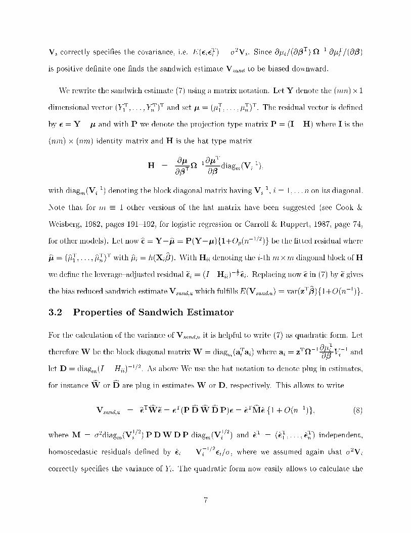
2 b�i. Replacing now b� in (7) by e� givesthe bias reduced sandwich estimateVsand;u which ful�llsE(Vsand;u) = var(zT b�)f1+O(n�1)g.3.2 Properties of Sandwich Estimator
For the calculation of the variance of Vsand;u it is helpful to write (7) as quadratic form. Let
thereforeW be the block diagonal matrixW = diagm(aTi ai) where ai = zT�1
@�Ti@� V �1i and
let D = diagm(I �Hii)�1=2. As above We use the hat notation to denote plug in estimates,
for instance cW or cD are plug in estimates W or D, respectively. This allows to write
Vsand;u = e�TcWe� = �T(PcD cW cDP)� = _�TcM _� f1 +O(n�1)g; (8)
where M = �2diagm(V1=2i )PDWDP diagm(V
1=2i ) and _�T = (_�T1 ; : : : ; _�
Tn ) independent,
homoscedastic residuals de�ned by _�i = V�1=2i �i=�, where we assumed again that �2Vi
correctly speci�es the variance of Yi. The quadratic form now easily allows to calculate the
7
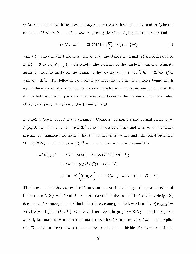
variance of the sandwich variance. Let mkl denote the k; l-th element ofM and let _�k be the
elements of _� where k; l = 1; 2; : : :mn. Neglecting the e�ect of plug-in estimates we �nd
var(Vsand;u) = 2tr(MM) +Xk
fE( _�4k)� 3gm2kk (9)
with tr(�) denoting the trace of a matrix. If _�k are standard normal (9) simpli�es due to
E( _�4k) = 3 to var(Vsand;u) = 2tr(MM): The variance of the sandwich variance estimate
again depends distinctly on the design of the covariates due to @�Ti =@� = Xi@h(�)=@�
with � = XTi �. The following example shows that this variance has a lower bound which
equals the variance of a standard variance estimate for n independent, univariate normally
distributed variables. In particular the lower bound does neither depend on m, the number
of replicates per unit, nor on p, the dimension of �.
Example 3 (lower bound of the variance): Consider the multivariate normal model Yi �N(XT
i �; �2I), i = 1; : : : ; n, with XT
i as m � p design matrix and I as m � m identity
matrix. For simplicity we assume that the covariates are scaled and orthogonal such that
=P
iXiXTi = nI. This gives
Pi a
Ti ai = n and the variance is obtained from
varfVsand;ug = 2�4tr(MM) = 2tr(WW)f1 +O(n�1)g
= 2n�4�4Xi
(aTi ai)2f1 +O(n�1)g
� 2n�5�4 X
i
aTi ai
!2
f1 +O(n�1)g = 2n�3�4f1 +O(n�1)g:
The lower bound is thereby reached if the covariates are individually orthogonal or balanced
in the sense XiXTi = I for all i. In particular this is the case if the individual design Xi
does not di�er among the individuals. In this case one gets the lower bound var(Vsand;u) =
2�4=fn2(n� 1)gf1 +O(n�1)g. One should note that the property XiXTi = I either requires
m > 1, i.e. one observes more than one observation for each unit, or if m = 1 it implies
that Xi � 1, because otherwise the model would not be identi�able. For m = 1 the simple
8
univariate normal model yi � N(�; �2) results with � as unknown constant mean and the
resulting variance estimate b�2 = Pi(yi� �y)2=(n� 1). This in turn implies a lower bound for
the quantiles used for the calculation of con�dence intervals, as will be discussed in the next
section.
For the calculation of var(Vsand;u) in (9) we neglected the variability occuring due to plug-
in estimation of �̂. If however the variance function V (�) is not constant both estimates
Vsand;u and Vmodel have a variance greater than zero. The next two examples show how
the additional variance occuring from the plug in estimates e�ects the relative eÆciency
var(Vsand)=var(Vmodel). We consider univariate Poisson and Logistic regression models, a
general discussion is given in the appendix.
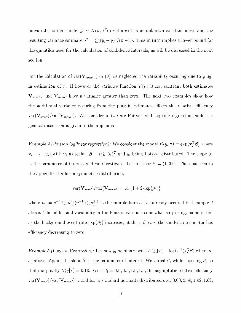
Example 4 (Poisson loglinear regression): We consider the model E(yijx) = exp(xTi �) where
xi = (1; ui) with ui as scalar, � = (�0; �1)T and yi being Poisson distributed. The slope �1
is the parameter of interest and we investigate the null case � = (1; 0)T. Then, as seen in
the appendix if u has a symmetric distribution,
var(Vsand)=var(Vmodel) = �nf1 + 2 exp(�0)g
where �n = n�1P
i u4i =(n
�1Pi u
2i )
2 is the sample kurtosis as already occured in Example 2
above. The additional variability in the Poisson case is a somewhat surprising, namely that
as the background event rate exp(�0) increases, at the null case the sandwich estimator has
eÆciency decreasing to zero.
Example 5 (Logistic Regression): Let now yi be binary with E(yijx) = logit�1(xTi �) where xi
as above. Again, the slope �1 is the parameter of interest. We varied �1 while choosing �0 so
that marginally E(yjx) = 0:10. With �1 = 0:0; 0:5; 1:0; 1:5, the asymptotic relative eÆciency
var(Vsand)=var(Vmodel) varied for ui standard normally distributed over 3:00; 2:59; 1:92; 1:62,
9

respectively. When ui comes from a Laplace distribution (with unit variance), the cor-
responding eÆciencies are 6:00; 4:36; 3:31; 2:57. Note that in both cases, at the null case
�1 = 0, the eÆciency of the sandwich estimator is exactly the same as the linear regression
problem. This is no numerical uke, and in fact can be shown to hold generally when u has
a symmetric distribution.
The above two example show that the loss of eÆciency of the sandwich variance estimate in
non normal models di�ers and can be worse compared to normal models. In the appendix
we discuss this point in more generality.
4 Con�dence Intervals based on Sandwich Variance Estimates
4.1 The Property of Undercoverage
In the following section we investigate the e�ect of the additional variability of the sandwich
variance estimate on the coverage probability of con�dence intervals. As one would expect the
excess variability of the sandwich estimate is directly re ected in undercoverage of con�dence
intervals. Let � = zT� be the unknown parameter of interest and let b� = zT b� be an unbiased,
n1=2{consistent estimate of �. We consider con�dence intervals based on the (asymptotic)
normality of �̂, i.e. we investigate the symmetrical 1 � � con�dence intervals CI(�2; �) :=
[�̂ � zp�=pn] where �2=n = var(�̂) and zp as p = 1 � �=2 quantile of the standard normal
distribution. If �2 is estimated by an unbiased variance estimate �̂2 it is well known that
the con�dence interval CI(b�2; �) shows undercoverage and typically t-distribution quantiles
are used instead of normal quantiles. The following theorem shows how the variance of the
variance estimate b�2 directly e�ects the undercoverage.
Theorem 2: Under the assumptions from above and assuming that �̂2 and �̂ are (asymp-
totically) independent the coverage probability of the 1 � � con�dence interval CI(b�2; �)
10

equals
Pf� 2 CI(b�2; �)g = 1� �� �(zp)var(�̂2)
z3p + zp
8�4
!+O(n�3=2) (10)
where �(�) is the standard normal distribution density.
The proof of the theorem is obtained by Edgeworth expansion and given in the appendix.
One should note that the postulated assumption of independence of b�2 and b� holds in a
normal regression model if b�2 is calculated from �tted residuals. Hence it holds for sandwich
variance estimates. In the non-normal case we have to rely on asymptotic independence. It
is seen from (10) that for � small, i.e. p large such that zp > 1, the coverage probability
of the con�dence interval falls below the the nominal value. Moreover, the undercoverage
increases linearly with the variance of the variance estimate b�2. Using the results of Theorem1 we therefore �nd that the sandwich estimator can be expected to have lower coverage
probability than the model based variance. Moreover, t�distribution quantiles instead of
normal quantiles do not correct the undercoverage, as seen below.
4.2 A Simple Coverage Adjustment
Formula (10) can be employed to construct a simple coverage correction for con�dence in-
tervals. Instead of using the quantile zp directly we suggest to choose ep > p and make use
of the zep quantile. We thereby select ep such that P (� 2 [�̂ � z~pb�]) = p holds, i.e. with (10)
we solve
p = ep� �(zep)var(b�2)z3ep + zep8�4
(11)
for ~p. Though equation (11) does not allow for an analytical solution for ep, a numerical
solution is easily calculated by iteration. It should be noted that ~p depends on p which is
however suppressed in the notation.
Example 6 (t-distribution quantiles): We demonstrate the above correction in a setting
11
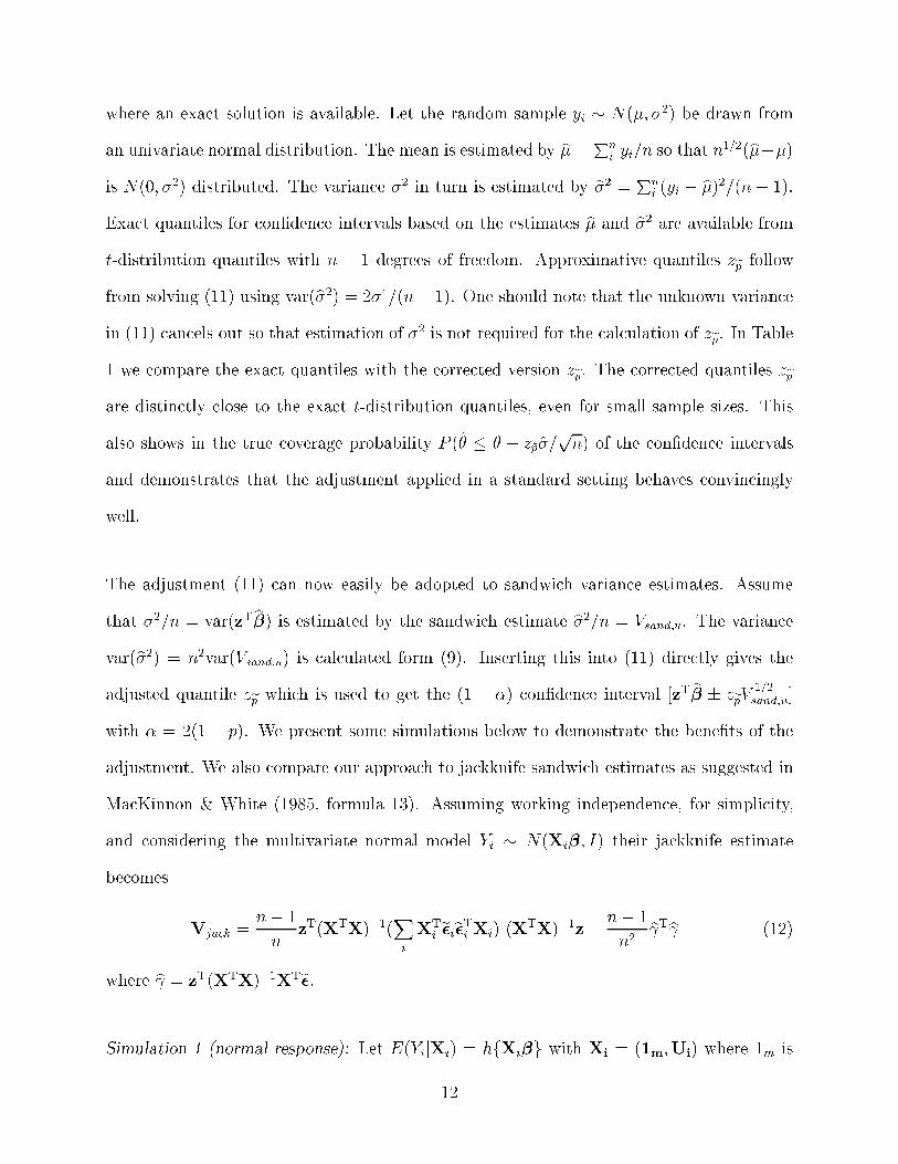
where an exact solution is available. Let the random sample yi � N(�; �2) be drawn from
an univariate normal distribution. The mean is estimated by b� =Pn
i yi=n so that n1=2(b���)is N(0; �2) distributed. The variance �2 in turn is estimated by b�2 = Pn
i (yi � b�)2=(n� 1).
Exact quantiles for con�dence intervals based on the estimates b� and b�2 are available fromt-distribution quantiles with n � 1 degrees of freedom. Approximative quantiles zep follow
from solving (11) using var(b�2) = 2�4=(n� 1). One should note that the unknown variance
in (11) cancels out so that estimation of �2 is not required for the calculation of zep. In Table
1 we compare the exact quantiles with the corrected version zep. The corrected quantiles zepare distinctly close to the exact t-distribution quantiles, even for small sample sizes. This
also shows in the true coverage probability P (�̂ � � + z~p�̂=pn) of the con�dence intervals
and demonstrates that the adjustment applied in a standard setting behaves convincingly
well.
The adjustment (11) can now easily be adopted to sandwich variance estimates. Assume
that �2=n = var(zT b�) is estimated by the sandwich estimate b�2=n = Vsand;u. The variance
var(b�2) = n2var(Vsand;u) is calculated form (9). Inserting this into (11) directly gives the
adjusted quantile zep which is used to get the (1 � �) con�dence interval [zT b� � zepV 1=2sand;u]
with � = 2(1 � p). We present some simulations below to demonstrate the bene�ts of the
adjustment. We also compare our approach to jackknife sandwich estimates as suggested in
MacKinnon & White (1985, formula 13). Assuming working independence, for simplicity,
and considering the multivariate normal model Yi � N(Xi�; I) their jackknife estimate
becomes
Vjack =n� 1
nzT(XTX)�1(
Xi
XTi e�ie�Ti Xi) (X
TX)�1z� n� 1
n2b Tb (12)
where b = zT(XTX)�1XTe�.
Simulation 1 (normal response): Let E(YijXi) = hfXi�g with Xi = (1m;Ui) where 1m is
12
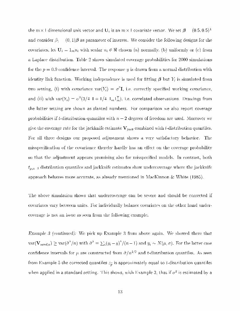
the m�1 dimensional unit vector and Ui is an m�1 covariate vector. We set � = (0:5; 0:5)T
and consider �1 = (0; 1)� as parameter of interest. We consider the following designs for the
covariates, let Ui = 1mui with scalar ui 2 < chosen (a) normally, (b) uniformly or (c) from
a Laplace distribution. Table 2 shows simulated coverage probabilities for 2000 simulations
for the p = 0:9 con�dence interval. The response y is drawn from a normal distribution with
identity link function. Working independence is used for �tting � but Yi is simulated from
two setting, (i) with covariance var(Yi) = �2I, i.e. correctly speci�ed working covariance,
and (ii) with var(Yi) = �2(3=4 I + 1=4 1m1Tm), i.e. correlated observations. Drawings from
the latter setting are shown as slanted numbers. For comparison we also report coverage
probabilities if t-distribution quantiles with n� 2 degrees of freedom are used. Moreover we
give the coverage rate for the jackknife estimateVjack combined with t-distribution quantiles.
For all three designs our proposed adjustment shows a very satisfactory behavior. The
misspeci�cation of the covariance thereby hardly has an e�ect on the coverage probability
so that the adjustment appears promising also for misspeci�ed models. In contrast, both
tp;n�2 distribution quantiles and jackknife estimates show undercoverage where the jackknife
approach behaves more accurate, as already mentioned in MacKinnon & White (1985).
The above simulation shows that undercoverage can be severe and should be corrected if
covariates vary between units. For individually balance covariates on the other hand under-
coverage is not an issue as seen from the following example.
Example 3 (continued): We pick up Example 3 from above again. We showed there that
var(Vsand;u) � var(b�2=n) with b�2 = Pi(yi� �y)2=(n�1) and yi � N(�; �). For the latter case
con�dence intervals for � are constructed from �̂=n1=2 and t-distribution quantiles. As seen
from Example 5 the corrected quantiles zep is approximately equal to t-distribution quantiles
when applied in a standard setting. This shows, with Example 3, that if �2 is estimated by a
13
sandwich estimate one obtains zep � tp;n�1, at least approximately with tp;n�1 as p quantile of
the t-distribution with n�1 degrees of freedom. If the design is individually balanced we saw
above that the lower bound of the variance is reached. This implies whenever the individual
design Xi does not di�er among the individuals, i.e. does not depend on i, one should use t
distribution quantiles with n� 1 degrees of freedom when constructing con�dence intervals
based on sandwich variance estimates. Consequently, undercoverage is not an issue in this
case.
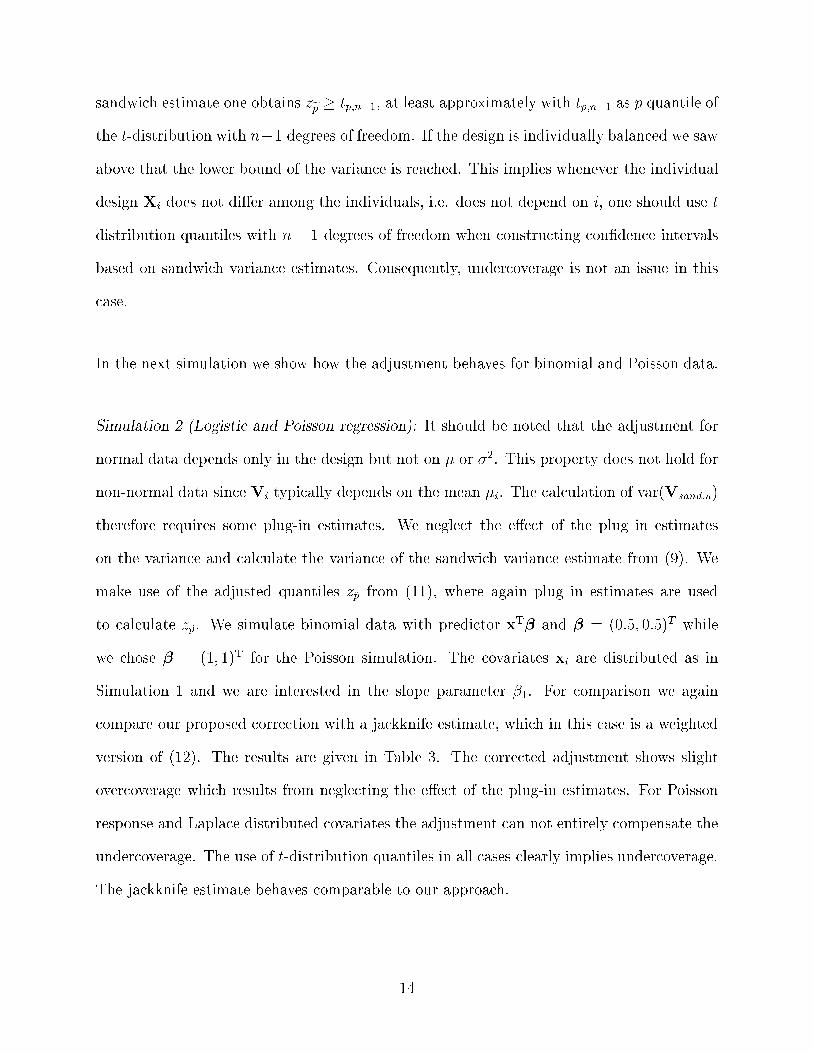
In the next simulation we show how the adjustment behaves for binomial and Poisson data.
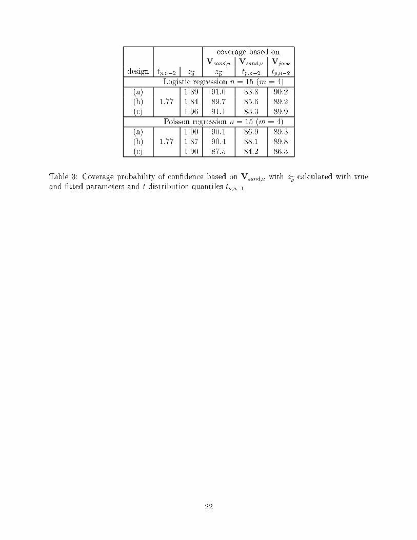
Simulation 2 (Logistic and Poisson regression): It should be noted that the adjustment for
normal data depends only in the design but not on � or �2. This property does not hold for
non-normal data since Vi typically depends on the mean �i. The calculation of var(Vsand;u)
therefore requires some plug-in estimates. We neglect the e�ect of the plug in estimates
on the variance and calculate the variance of the sandwich variance estimate from (9). We
make use of the adjusted quantiles z~p from (11), where again plug in estimates are used
to calculate z~p. We simulate binomial data with predictor xT� and � = (0:5; 0:5)T while
we chose � = (1; 1)T for the Poisson simulation. The covariates xi are distributed as in
Simulation 1 and we are interested in the slope parameter �1. For comparison we again
compare our proposed correction with a jackknife estimate, which in this case is a weighted
version of (12). The results are given in Table 3. The corrected adjustment shows slight
overcoverage which results from neglecting the e�ect of the plug-in estimates. For Poisson
response and Laplace distributed covariates the adjustment can not entirely compensate the
undercoverage. The use of t-distribution quantiles in all cases clearly implies undercoverage.
The jackknife estimate behaves comparable to our approach.
14

5 Discussion
We showed above that sandwich variance estimates carry the problem of being less eÆcient
than model based variance estimates. The loss of eÆciency thereby depends on the design
and for standard cases it is directly proportional to the inverse of the kurtosis of the design
points. For non normal data additional components beside the kurtosis in uence the loss
of eÆciency. The variance of the sandwich variance estimate directly e�ects the coverage
probability of con�dence intervals and undercoverage is implied if the design di�ers among
the independent individuals. A simple adjustment which depends on the design is suggested
which allows to correct the de�cit of undercoverage.
A Technical Details
A.1 Proof of Examples 4 and 5
Below we derive the relative eÆciency in quasi likelihood models in the following. For sim-
plicity of notation we consider univariate regression models of the form E(yijxi) = �(xTi �) =
h(xTi �) with xTi as 1 � p vector. The variance of yi is given by var(yijxi) = �2V f�(xTi �)g
where V (�) is a known variance function. In some problems, �2 is estimated, which we
indicate by setting � = 1, while when �2 is known we set � = 0. We denote the deriva-
tives of functions by superscripts, e.g. �(l)(�) = @l�(�)=(@�)l. Let us assume that the
variance is correctly speci�ed, i.e. var(yijxi) = �2V f�(xTi �)g, so that with expansion (6)
we get var(n1=2zT�) = �2zTn(�)z where n(�) = n�1Pn
i=1 xixTi Q(x
T�) with Q(�) =
f�(1)(�)g2=V (�). The model based variance estimator is Vmodel = b�2(b�)zT�1n (b�)z; whereb�2(�) = �n�1
nXi=1
fyi � �(xT�)g2=V (xT�) + �2(1� �):
De�ning Bn(�) = n�1Pn
i=1 xixTi M(xTi �)fyi � �(xTi �)g2 and M(�) = f�(1)(�)=V (�)g2, the
sandwich estimator is written as Vsand = zT�1n (b�)Bn(b�)�1n (b�)z:For the derivation of the following theorem we need some additional notation. Let Rn =
�n�1Pn
i=1 g(xTi �)x
Ti where g(�) = (@=@�) logfV (�)g; �i = fyi � �(xTi �)g=V 1=2(xTi �); qin =
15
xTi �1n (�)z; an = zT�1n (�)z; Cn = n�1
Pni=1 q
2inQ
(1)(xTi �)xi and
`in = �1n (�)xi�(1)(xTi �)=V
1=2(xTi �);
vi = fyi � �(xTi �)g2M(xTi �)� �2Q(xTi �);
Kn = n�1nX
i=1
q2inV (xTi �)M
(1)(xTi �)xi:
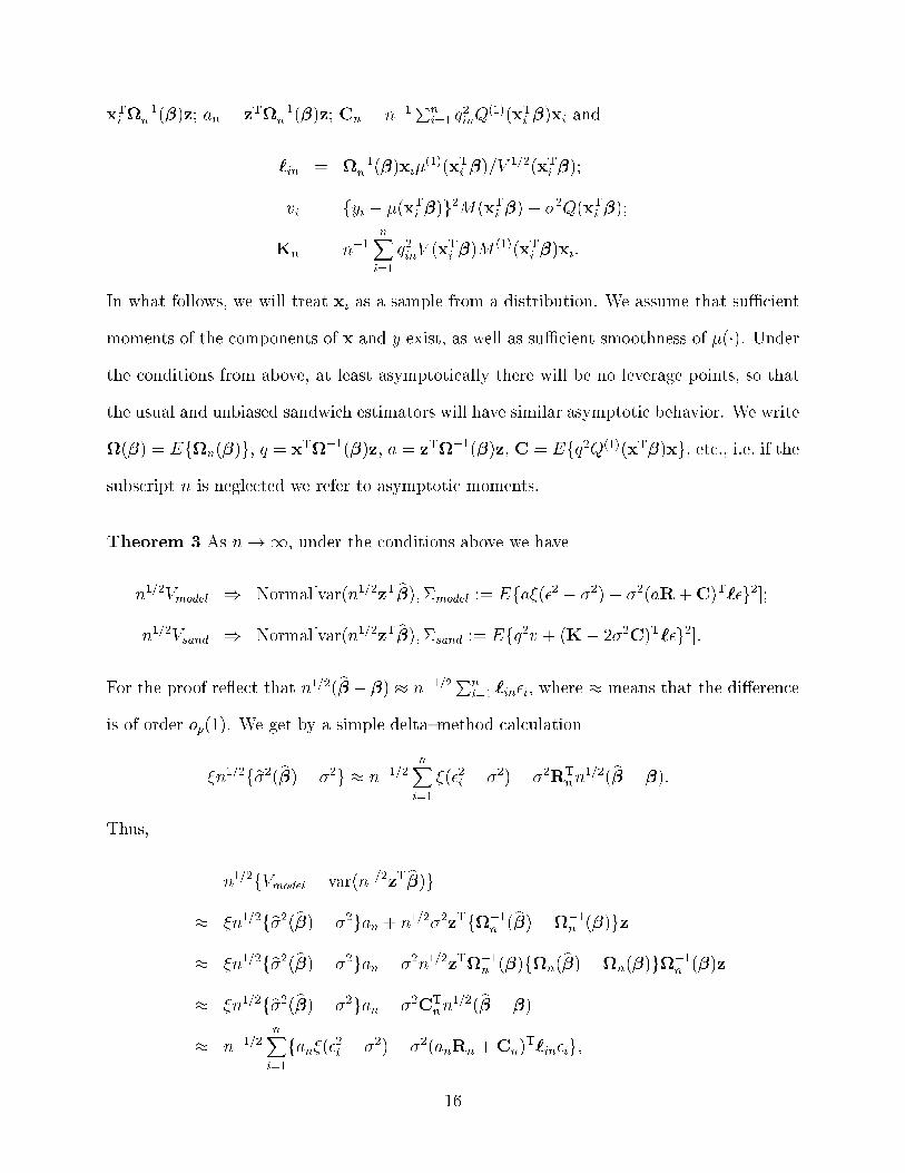
In what follows, we will treat xi as a sample from a distribution. We assume that suÆcient
moments of the components of x and y exist, as well as suÆcient smoothness of �(�). Underthe conditions from above, at least asymptotically there will be no leverage points, so that
the usual and unbiased sandwich estimators will have similar asymptotic behavior. We write
(�) = Efn(�)g, q = xT�1(�)z, a = zT�1(�)z, C = Efq2Q(1)(xT�)xg, etc., i.e. if thesubscript n is neglected we refer to asymptotic moments.
Theorem 3 As n!1, under the conditions above we have
n1=2Vmodel ) Normal[var(n1=2zT b�);�model := Efa�(�2 � �2)� �2(aR+C)T`�g2];
n1=2Vsand ) Normal[var(n1=2zT b�);�sand := Efq2v + (K� 2�2C)T`�g2]:
For the proof re ect that n1=2(b�� �) � n�1=2Pn
i=1 `in�i, where � means that the di�erence
is of order op(1). We get by a simple delta{method calculation
�n1=2fb�2(b�)� �2g � n�1=2nX
i=1
�(�2i � �2)� �2RTnn
1=2(b� � �):
Thus,
n1=2fVmodel � var(n1=2zT b�)g� �n1=2fb�2(b�)� �2gan + n1=2�2zTf�1n (b�)��1n (�)gz
� �n1=2fb�2(b�)� �2gan � �2n1=2zT�1n (�)fn(b�)�n(�)g�1n (�)z
� �n1=2fb�2(b�)� �2gan � �2CTnn
1=2(b� � �)
� n�1=2nX
i=1
fan�(�2i � �2)� �2(anRn +Cn)T`in�ig;
16

which shows the �rst part of Theorem 4.
We now turn to the sandwich estimator, and note that Bn(�) � �2n(�) = Op(n�1=2).
Because of this, we have that
n1=2fVsand � var(n1=2zT b�)g � �2�2n1=2zT�1n (�)fn(b�)�n(�)g�1n (�)z
+n1=2zT�1n (�)fBn(b�)� �2n(�)g�1n (�)z
� �2�2n�1=2nX
i=1
CTn`in�i + n�1=2
nXi=1
q2in[M(XTib�)fYi � �(XT
ib�)g2 � �2Q(xTi �)]
� �2�2n�1=2nX
i=1
CTn`in�i + n�1=2
nXi=1
q2invi + n�1nX
i=1
q2iM(1)(xTi �)XifYi � �(xTi �)g2n1=2(b� � �)
� �2�2n�1=2nX
i=1
CTn`in�i + n�1=2
nXi=1
q2invi + n�1nX
i=1
q2iM(1)(xTi �)XiV (x
Ti �)n
1=2(b� � �)
� n�1=2nX
i=1
(�2�2CTn`in�i + q2i vi +KT
n`in�i);
as claimed.
Theorem 3 can now be used to prove the statements listed in Examples 4 and 5. For
the logistic case we have V (�) = �(1)(�) = Q(�) = �(�)f1� �(�)g, �2 = 1, � = 0, Rn = 0,
Q(1)(�) = �(1)(�)f1�2�(�)g. All the terms in Theorem 3 can then be computed by numerical
integration which gives the numbers presented in Example 5.
For the Poisson case it is easily veri�ed that (�) = exp(�0)I2, where I2 is the identity
matrix. Also, q = U exp(��0), xT� = �0, Q(1)(xT�) = exp(�0), C = exp(��0)(1; 0)T,
` = exp(��0=2)(1; U)T, � = fY � exp(�0)g= exp(�0=2) and hence �model = exp(�3�0).
Let � = exp(�0). Then E(Y2) = �+�2, E(Y 3) = �3+3�2+�, and E(Y 4) = �4+6�3+7�2+�.
If we de�ne Z = Y � �, then E(Z) = 0, E(Z2) = E(Z3) = � and E(Z4) = 3�2 + �.
Further, M(�) = 1, M (1)(�) = 0, K = 0. A detailed calculation then shows that �sand =
2� exp(�2�0) + � exp(�3�0) which shows the relative eÆciency given in Example 4.
17

A.2 Proof of Theorem 2
We give the proof of Theorem 2 in a rather general fashion. Let F (�) denote the distributionof �̂� � and bF (�) be a corresponding estimate of F (�). Let �l and b�l be the l-th cumulant of
F (�) and bF (�) respectively, l = 1; 2; : : :. We assume that �1 = b�1 = 0 and �l = O(n�(l�2)=2)
which mirrors standard n1=2{asymptotics. We also postulate that b�l is a consistent estimate
of �l, i.e. b�l��l = Op(n� 1
2 )O(�l) and we assume that the cumulants b�l are independent of �̂for l = 2; 3; : : :. Let bvp denote the empirical p quantile, i.e. bF (bvp) = p. As seen below, since
b�l and b� are assumed to be independent one gets bvp and b� independent. Our intention is to
calculate the true coverage probability Pf(�̂ � �) � v̂pg. Let Hv̂p(�) denote the distributionfunction of v̂p. One �nds, by making use of the above independence assumption
Pf(�̂ � �) � v̂pg =ZPf(�̂ � �) � vjv̂p = v)dHv̂p(v)
=ZF (v)dHv̂p = EfF (v̂p)g:
Hence, we have to calculate the expectation of F (v̂p) to obtain the coverage probability.
Simple expansion about the true quantile vp yields
F (bvp) = F (vp) + F (1)(vp)(bvp � vp) +1
2F (2)(vp)(bvp � vp)
2 + : : : (13)
where F (l)(�) denotes the l-th derivative of F (�). The calculation of the expectation requires
an expansion for bvp which is derived in the following (see also Hall, 1992, for a similar
expansion). We �rst expand bF (�) by Edgeworth expansion about F (�). Following McCullagh
(1987, page 144{47) this yields bF (v) = F (v) + b�F (v) where the correction term equals
b�F (v) =Xl�2
(�1)lF(l)(v)
l!bÆl (14)
with Æ̂2 = �̂2��2; Æ̂3 = �̂3��3 and Æ̂4 = �̂4��4+3Æ̂22 and so on. Let G(p) = F�1(p) denote
the inverse distribution function. The empirical quantile p = bF (bvp) = F (bvp) + b�F (bvp) isthen expanded by
bvp = Gfp� b�F (bvp)g18

= G(p)�G(1)(p)f b�F (vp) + b�(1)F (vp)(bvp � vp) + : : :g
+1
2G(2)(p)f b�F (vp) + b�(1)
F (vp)(bvp � vp) + : : :g2 + : : : (15)
where b�(l)F (v) = @l b�F (v)=(@v)
l. With vp = G(p) as true quantile we can solve (15) for
(bvp � vp) by series inversion. This permits the �rst order approximation
bvp � vp = f1 +G(1)(p) b�(1)F (vp)g�1f�G(1)(p) b�F (vp) +
1
2G(2)(p) b�F (vp)
2g+O( b�3F )
= �G(1)(p) b�F (vp) +1
2G(2)(p) b�F (vp)
2 (16)
+G(1)2(p) b�(1)(vp) b�F (vp) +O( b�3F ):
In O( b�3F ) we collect components of the third power of b�F (vp) or its derivatives, e.g. b�F (vp)
3
is a representative. Re ecting that b�F (vp) is dominated by bÆ2 = b�2 � �2 provides O( b�3F ) =
Op(n� 3
2 )O(�2) so that O( b�3F ) collects components of negligible order. Inserting (16) in (13)
yields
F (bvp) = F (vp)
+F (1)(vp)f�G(1)(p) b�F (vp) +1
2G(2)(p) b�F (vp)
2 +G(1)2(p) b�(1)F (vp) b�F (vp)g
+1
2F (2)(vp)G
(1)2(p) b�F (vp)2 +O( b�3
F )
which simpli�es with G(1)(p) = 1=F (1)(vp) and G(2)(p) = �F (2)(vp)=F(1)(vp)
3 to
F (bvp) = p� b�F (vp) +1
F (1)(vp)b�(1)(vp) b�F (vp) +O( b�3
F ):
Assuming unbiased estimates for the cumulants we �nd with (14)Ef�̂p(vp)g= 1=24F (4)(vp)var(bÆ2)f1+O(n�1=2)g and E( b�(1)(vp) b�F (vp)) = 1=4F (2)(vp)F
(3)(vp)var(bÆ2)f1+O(n�1=2)g which �nally
yields
EfF (bvp)g = p+ var(�̂2)
(�1
8F (4)(vp) +
1
4
F (2)(vp)F(3)(vp)
F (1)(vp)
)f1 +O(n�1=2)g: (17)
Taking now F (v) = �(v=�) with �(�) as standard normal distribution function and F̂ (v) =
�(v=b�), where �̂2 = �̂2 is an estimate of the second order cumulant, gives with vp = zp�,
v̂p = zp�̂ and (17) formula (10) in Theorem 2.
19
References
Breslow, N. (1990). Test of hypotheses in overdispersion regression and other quasilikelihoodmodels. Journal of the American Statistical Association, 85, 565{571.
Cook, R. D. & Weisberg, S. (1982). Residuals and In uence in Regression. Chapman &Hall, London.
Diggle, P. J., Liang, K. Y. & Zeger, S. L. (1994). Analysis of Longitudinal Data. ClarendonPress, Oxford.
Efron, B. (1986). Discussion of the paper by C. F. J. Wu \Jackknife, bootstrap and otherresampling methods in statistics". Annals of Statistics, 14, 1301{1304.
Firth, D. (1992). Discussion of the paper by Liang, Zeger & Qaqish \Multivariate regressionanalysis for categorical data". Journal of the Royal Statistical Society, Series B, 54, 24{26.
Gourieroux, C., Monfort, A. and Trognon A. (1984). Pseudo maximum likelihood methods:applications to Poisson models. Econometrica, 52, 701{720.
Hall, P. (1992). The Bootstrap and Edgeworth Expansion. Springer Verlag, Berlin,New York.Hinkley, D. V. (1977). Jackkni�ng in unbalanced situations. Technometrics, 19, 285{292.Huber, P. J. (1967). The behavior of maximum likelihood estimation under nonstandard
conditions. Proceedings of the Fifth Berkeley Symposium on Mathematical Statistics and
Probability, 1, LeCam, L. M. and Neyman, J. editors. University of California Press, pp.221{233.
Liang, K. Y. & Zeger, S. L. (1986). Longitudinal data analysis using generalized linearmodels. Biometrika, 73, 13{22.
Liang, K. Y., Zeger, S. L. & Qaqish, B. (1992). Multivariate regression analysis for categor-ical data. Journal of the Royal Statistical Society, Series B, 54, 3{40.
MacKinnon, J. G., and White, H. (1985). Some heteroskedasticity-consistent covariancematrix estimators with improved �nite sample properties. Journal of Econometrics, 29,305{325.
McCullagh, P. (1987). Tensor methods in statistics. Chapman & Hall, London.McCullagh, P. (1992). Discussion of the paper by Liang, Zeger & Qaqish \Multivariate
regression analysis for categorical data". Journal of the Royal Statistical Society, Series
B, 54, 24{26.McCullagh, P. and Nelder, J.A. (1989). Generalized Linear Models. Chapman and Hal, New
York.Rothenberg, T.J. (1988). Approximative power functions for some robust tests of regression
coeÆcients. Econometrica, 56, 997{1019.White, H. (1982). Maximum likelihood estimation of misspeci�ed models. Econometrica,
50, 1{25.Wu, C. F. J. (1986). Jackknife, bootstrap and other resampling methods in statistics. Annals
of Statistics, 14, 1261{1350.Wedderburn, R. W. M (1974). Quasi-likelihood functions, generalized linear models, and
the Gauss-Newton method. Biomtrika, 61, 439{447.
20

p tp;n�1 zep P (�̂ � � + z~p�̂=pn)
n = 5.90 1.533 1.551 .902.95 2.132 2.095 .948.975 2.776 2.543 .968
n = 15.90 1.345 1.346 .900.95 1.761 1.761 .950.975 2.145 2.137 .975
Table 1: Comparison of coverage probability based on zep and t-distribution quantiles tp;n�1for n� 1 degrees of freedom
coverage based onVsand;u Vsand;u Vjack
design tp;n�2 zep zep tp;n�2 tp;n�2n = 10 (m = 4)
(a) 2.10 88.8 (88.5) 84.9 (84.9) 86.4 (87.2)(b) 1.86 2.03 88.5 (90.2) 86.3 (87.5) 87.6 (89.0)(c) 2.18 88.9 (89.0) 84.2 (84.6) 86.7 (86.8 )
n = 20 (m = 4)(a) 1.86 89.5 (89.7) 87.0 (87.8) 88.3 (88.8)(b) 1.71 1.81 90.3 90.0) 88.5 88.4) 89.8 (89.9)(c) 1.94 90.0 (90.5) 86.5 (87.1) 88.2 (88.9)
Table 2: Coverage probability based on Vsand;u with zep and t distribution quantiles tp;n�1and jackknife estimate Vjack (Slanted numbers show simulations for correlated responses)
21
coverage based onVsand;u Vsand;u Vjack
design tp;n�2 zep zep tp;n�2 tp;n�2Logistic regression n = 15 (m = 4)
(a) 1.89 91.0 83.8 90.2(b) 1.77 1.84 89.7 85.6 89.2(c) 1.96 91.1 83.3 89.9
Poisson regression n = 15 (m = 4)(a) 1.90 90.1 86.9 89.3(b) 1.77 1.87 90.4 88.1 89.8(c) 1.90 87.5 84.2 86.3
Table 3: Coverage probability of con�dence based on Vsand;u with zep calculated with trueand �tted parameters and t distribution quantiles tp;n�1
22

This is the original Section 3.2. I incorporated the results given here in the previoussections. I put the Theorem in the appendix. Please see this as a proposal !!
A.3 Asymptotic Comparisons in the Univariate Case
We now derive an asymptotic comparison between the sandwich and usual estimators in aquasilikelihood model. The mean of Y given X is �(XT�) and its variance is �2V (XT�),where the functions �(�) and V (�) are known. In some problems, �2 is estimated, which weindicate by setting � = 1, while when �2 is known we set � = 0. The quasilikelihood estimateof � is the solution b� to
0 =nX
i=1
fYi � �(XTib�)gXi�
(1)(XTib�)=V (XT
ib�);
where in general the jth derivative of a function f(x) is denoted by f (j)(x).
The usual estimator of the covariance matrix of n1=2zT(b� � �) is
Vql = b�2(b�)zT�1n (b�)z;where n(�) = n�1
Pni=1XiX
Ti Q(x
Ti �); Q(x) = f�(1)(x)g2=V (x), and
b�2(�) = �n�1nXi=1
fYi � �(xTi �)g2=V (xTi �) + �2(1� �):
De�ning Bn(�) = n�1Pn
i=1XiXTi M(xTi �)fYi��(xTi �)g2 and M(x) = f�(1)(x)=V (x)g2, the
usual sandwich estimator is
Vsand = zT�1n (b�)Bn(b�)�1n (b�)z: (18)
Make the following de�nitions: Vasymp = �2zT�1n (�)z; Rn = �n�1Pn
i=1 g(xTi �)Xi;
g(x) = (@=@x) logfV (x)g; �i = fYi��(xTi �)g=V 1=2(xTi �); qin = XTi
�1n (�)z; an = zT�1n (�)z;
Cn = n�1Pn
i=1 q2inQ
(1)(xTi �)Xi and
`in = �1n (�)Xi�(1)(xTi �)=V
1=2(xTi �);
vi = fYi � �(xTi �)g2M(xTi �)� �2Q(xTi �);
Kn = n�1nX
i=1
q2inV (xTi �)M
(1)(xTi �)Xi:
In linear regression, we were able to perform exact calculations, and we did not rely onasymptotics. In quasilikelihood models, such exact calculations are not feasible, and asymp-totics are required. In what follows, we will treat the X's as a sample from a distribution,and terms without the subscript n will refer to probability limits. We will not write downformal regularity conditions, but essentially what is necessary is that suÆcient momentsof the components of X and Y exist, as well as suÆcient smoothness of �(�). Under such
23

conditions, at least asymptotically there will be no leverage points, so that the usual and un-biased sandwich estimators will have similar asymptotic behavior. Thus (�) = Efn(�)g,q = XT�1(�)z, a = zT�1(�)z, C = Efq2Q(1)(XT�)Xg, etc.Theorem 4: As n!1,
n1=2(Vql � Vasymp) ) Normal[0;�ql = Efa�(�2 � �2)� �2(aR+C)T`�g2];n1=2(Vsand � Vasymp) ) Normal[0;�sand = Efq2v + (K� 2�2C)T`�g2]:
The terms Vql and Vsand can be computed and compared in a few special cases with ascalar predictor where the slope is of interest, so that X = (1; U)T and � = (�0; �1)
T.
� In linear homoscedastic regression, �(x) = x, V (x) = 1. When U has a symmetricdistribution, then simple calculations show that �sand=�ql = �, the kurtosis of U , i.e.,� = E(U4)=fE(U2)g2. This is the asymptotic version of Theorems 2 and 3.
� In logistic regression, V (x) = �(1)(x) = Q(x) = �(x)f1 � �(x)g, �2 = 1, � = 0,
Rn = 0, Q(1)(x) = �(1)(x)f1 � 2�(x)g. All the terms in Theorem 4 can be computedby numerical integration. We have evaluated the expressions when U has a normal orLaplace distribution, both with variance 1. We varied �1 while choosing �0 so thatmarginally pr(Y = 1) = 0:10. With �1 = 0:0; 0:5; 1:0; 1:5, the asymptotic relative eÆ-ciency of the usual information covariance matrix estimate compared to the sandwichestimate when the predictors are normally distributed is 3:00; 2:59; 1:92; 1:62, respec-tively. When the predictors have a Laplace distribution, the corresponding eÆcienciesare 6:00; 4:36; 3:31; 2:57.
Note that in both these situations, at the null case �1 = 0, the eÆciency of the sandwichestimator is exactly the same as the linear regression problem. This is no numerical uke, and in fact can be shown to hold generally when U has a symmetric distribution.
� In Poisson loglinear regression, �(x) = V (x) = exp(x), �2 = 1, � = 0 and Rn = 0.Here we consider only the null case, so that �1 = 0. Then, as sketched in the appendix,if U has a symmetric distribution,
�sand=�ql = �+ 2� exp(�0):
This is a somewhat surprising result, namely that as the background event rate exp(�0)increases, at the null case the sandwich estimator has eÆciency decreasing to zero.
� More generally, at the null case the role of the kurtosis of the design becomes clear.
Let zTz = 1 and fZTfZ = nI. Then Q(x) = Q(�0) = Q, A = QI, M = Q=V ,g = (@=@�0) logfV (�0)g, R = �g(1; 0)T, q = U=Q, a = 1=Q, C = (Q(1)=Q2)(1; 0)T,` = Q�1=2(1; U), v = (�2 � �2)Q, K = (M (1)V=Q2)(1; 0)T and thus
�ql = Eh�(�2 � �2)=Q� �2f(�g=Q) + (Q(1)=Q2)gQ�1=2�
i2;
�sand = EhU2(�2 � �2)=Q+ f(VM (1)=Q2)� (2�2Q(1)=Q2)gQ�1=2�
i2:
The kurtosis of U arises because of fourth moments of U appear in the expression for�sand.
24

This is the remaining abstract. I also put the multivariate case here and left the univariatein the paper (appendix). Again I stress that I see this as a proposal and if you have a di�erentopinion please change the �le as you like.
B Asymptotic Expression for G�oran's Multivariate Case
This assumes that the working covaraince matrix is asymptotically correct.
Let Ci(�) = (@�Ti )=(@�), �i(�) = Yi � �(Xi�), Lin(�) = zT�1n (�)CTi (�)V
�1i (�),
n(�) = n�1P
iCTi (�)V
�1i (�)Ci(�), Min(�) = (@Lin(�)=(@�
T), qi(�) = LTin(�)�i(�),
QTn (�) = n�1
Pi L
Tin(�)Vi(�)Min(�). The sandwich estimator and the asymptotic variance
are, respectively,
Vsand = zT�1(b�)n�1 nXi=1
CTi (b�)V�1
i (b�)�i(b�)�Ti (b�)V�1i (b�)Ci(b�)�1n (b�)z;
Vasymp = zT�1(b�)n�1 nXi=1
CTi (b�)V�1
i (b�)CTi (b�)�1n (b�)z:
Remembering that �i(�) = �, Simple algebra shows that
n1=2(Vsand � Vasymp) = n�1=2nX
i=1
fLin(b�)� Lin(�)gT�i(b�)�Ti (b�)Lin(b�)+n�1=2
nXi=1
LTin(b�)f�i(b�)� �ig�Ti (b�)Lin(b�)
+n�1=2nXi=1
LTin(b�)�if�i(b�)� �igTLin(b�)
+n�1=2nXi=1
LTin(b�)�i�Ti fLin(b�)� Lin(�)g
+n�1=2nXi=1
LTin(b�)f�i�Ti �Vi(�)gLin(b�):
A simple expansion shows that
n1=2(Vsand � Vasymp) = n�1=2nX
i=1
LTin(b�)f�i�Ti �Vi(�)gLin(b�)
+2n�1nX
i=1
LTin(b�)�i�Ti Min(�)n
1=2(b� � �)g
+2n�1nX
i=1
LTin(b�)�iLT
in(b�)f�i(b�)� �ig+ op(1):
Since �i(b�) � �i � �Ci(�)(b� � �), it is easily seen that the last term in the previousexpression is op(1). Hence we have shown that
n1=2(Vsand � Vasymp) = n�1=2nXi=1
LTin(�)f�i�Ti �Vi(�)gLin(�)
25

+2n�1nXi=1
LTin(b�)Vi(�)Min(�)n
1=2(b� � �)g+ op(1):
De�ne Gn(�) = n�1P
i LTin(�)Vi(�)Min(�). Since we have that
n1=2(b� � �) = n�1=2nX
i=1
�1(�)Ci(�)V�1i (�)�i;
we have thus show that
n1=2(Vsand � Vasymp) = n�1=2nX
i=1
LTin(b�)f�i�Ti �Vi(�)gLin(b�)
+2n�1=2nXi=1
Gn(�)�1(�)Ci(�)V
�1i (�)�i;
as claimed.
B.1 Proof of Theorem 4
A standard quasilikelihood expansion gives n1=2(b� � �) � n�1=2Pn
i=1 `in�i, where � meansthat the di�erence is of order op(1). A simple delta{method calculation yields
�n1=2fb�2(b�)� �2g � n�1=2nX
i=1
�(�2i � �2)� �2RTnn
1=2(b� � �):
Thus,
n1=2(Vql � Vasymp) � �n1=2fb�2(b�)� �2gan + n1=2�2zTf�1n (b�)��1n (�)gz� �n1=2fb�2(b�)� �2gan � �2n1=2zT�1n (�)fn(b�)�n(�)g�1n (�)z
� �n1=2fb�2(b�)� �2gan � �2CTnn
1=2(b� � �)
� n�1=2nX
i=1
fan�(�2i � �2)� �2(anRn +Cn)T`in�ig;
which shows the �rst part of Theorem 4.
We now turn to the sandwich estimator, and note that Bn(�) � �2n(�) = Op(n�1=2).
Because of this, we have that
n1=2(Vsand � Vasymp) � �2�2n1=2zT�1n (�)fn(b�)�n(�)g�1n (�)z
+n1=2zT�1n (�)fBn(b�)� �2n(�)g�1n (�)z
� �2�2n�1=2nX
i=1
CTn`in�i + n�1=2
nXi=1
q2in[M(XTib�)fYi � �(XT
ib�)g2 � �2Q(xTi �)]
� �2�2n�1=2nX
i=1
CTn`in�i + n�1=2
nXi=1
q2invi + n�1nX
i=1
q2iM(1)(xTi �)XifYi � �(xTi �)g2n1=2(b� � �)
� �2�2n�1=2nX
i=1
CTn`in�i + n�1=2
nXi=1
q2invi + n�1nX
i=1
q2iM(1)(xTi �)XiV(xTi �)n1=2(b� � �)
� n�1=2nX
i=1
(�2�2CTn`in�i + q2i vi +KT
n`in�i);
as claimed.
26

B.2 Calculations in the Poisson Case
It is easily veri�ed that (�) = exp(�0)I2, where I2 is the identity matrix. Also, q =U exp(��0),XT� = �0, Q
(1)(XT�) = exp(�0),C = exp(��0)(1; 0)T, ` = exp(��0=2)(1; U)T,� = fY � exp(�0)g= exp(�0=2) and hence �ql = exp(�3�0).
Let � = exp(�0). Then E(Y2) = �+�2, E(Y 3) = �3+3�2+�, and E(Y 4) = �4+6�3+7�2+�.
If we de�ne Z = Y � �, then E(Z) = 0, E(Z2) = E(Z3) = � and E(Z4) = 3�2 + �.Further, M(x) = 1, M (1)(x) = 0, K = 0. A detailed calculation then shows that �sand =2� exp(�2�0) + � exp(�3�0).
27
Recommended