1
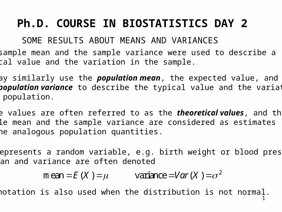
Ph.D. COURSE IN BIOSTATISTICS DAY 2
SOME RESULTS ABOUT MEANS AND VARIANCESThe sample mean and the sample variance were used to describe a typical value and the variation in the sample.
We may similarly use the population mean, the expected value, and the population variance to describe the typical value and the variation in a population.
These values are often referred to as the theoretical values, and the sample mean and the sample variance are considered as estimates of the analogous population quantities.
If X represents a random variable, e.g. birth weight or blood pressure, the mean and variance are often denoted
2mean ( ) variance ( )E X Var X
The notation is also used when the distribution is not normal.
2
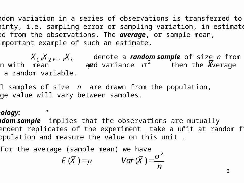
The random variation in a series of observations is transferred to uncertainty, i.e. sampling error or sampling variation, in estimates computed from the observations. The average, or sample mean, is an important example of such an estimate.
Let denote a random sample of size n from a population with mean and variance then the average is itself a random variable.
If several samples of size n are drawn from the population, the average value will vary between samples.
1 2, , , nX X X 2 X
Terminology: A ”random sample” implies that the observations are mutually independent replicates of the experiment ”take a unit at random from the population and measure the value on this unit”.
For the average (sample mean) we have2
( ) ( )E X Var Xn
3
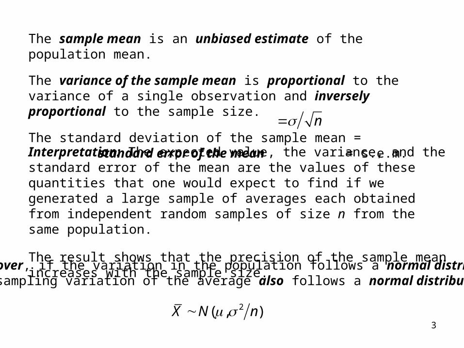
The sample mean is an unbiased estimate of the population mean. The variance of the sample mean is proportional to the variance of a single observation and inversely proportional to the sample size.
The standard deviation of the sample mean = standard error of the mean = s.e.m. n
Interpretation: The expected value, the variance, and the standard error of the mean are the values of these quantities that one would expect to find if we generated a large sample of averages each obtained from independent random samples of size n from the same population.
The result shows that the precision of the sample mean increases with the sample size.
Moreover, if the variation in the population follows a normal distribution the sampling variation of the average also follows a normal distribution
2( , )X N n
4
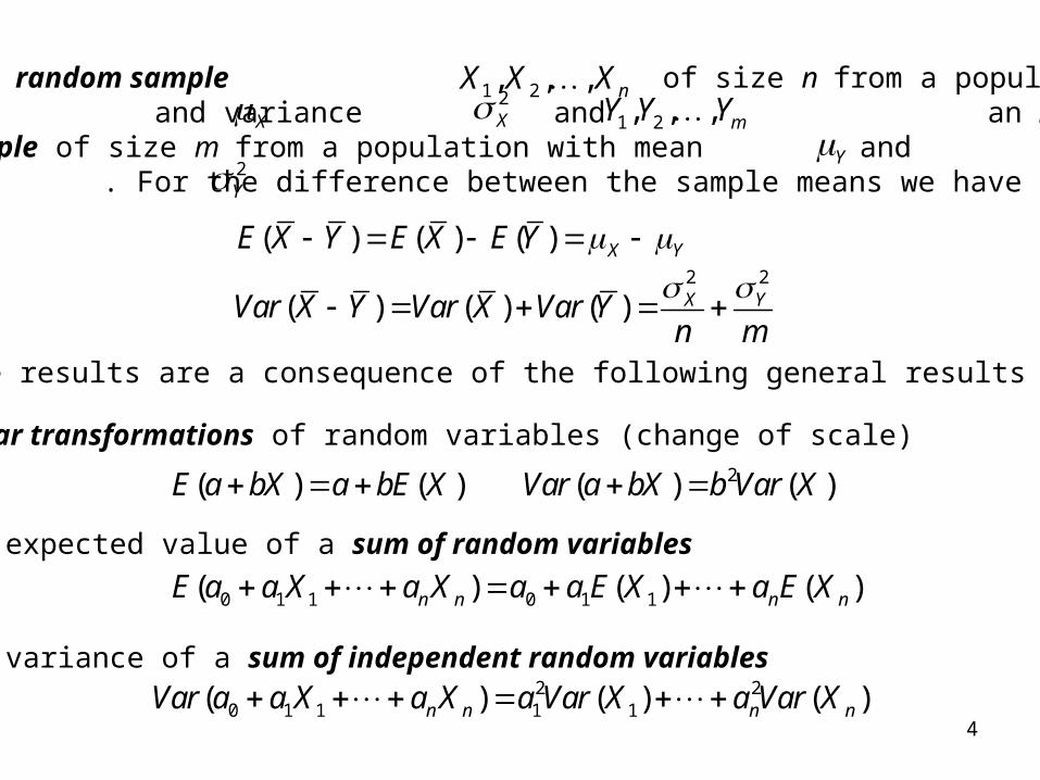
Consider a random sample of size n from a population with mean and variance and an independent random sample of size m from a population with mean and variance . For the difference between the sample means we have
1 2, , , nX X X1 2, , , mY Y Y
Y2XX
2Y
2 2
( ) ( ) ( )
( ) ( ) ( )
X Y
X Y
E X Y E X E Y
Var X Y Var X Var Yn m
These results are a consequence of the following general results
• Linear transformations of random variables (change of scale)
• The expected value of a sum of random variables
• The variance of a sum of independent random variables
2( ) ( ) ( ) ( )E a bX a bE X Var a bX b Var X
0 1 1 0 1 1( ) ( ) ( )n n n nE a a X a X a a E X a E X
2 20 1 1 1 1( ) ( ) ( )n n n nVar a a X a X a Var X a Var X
5
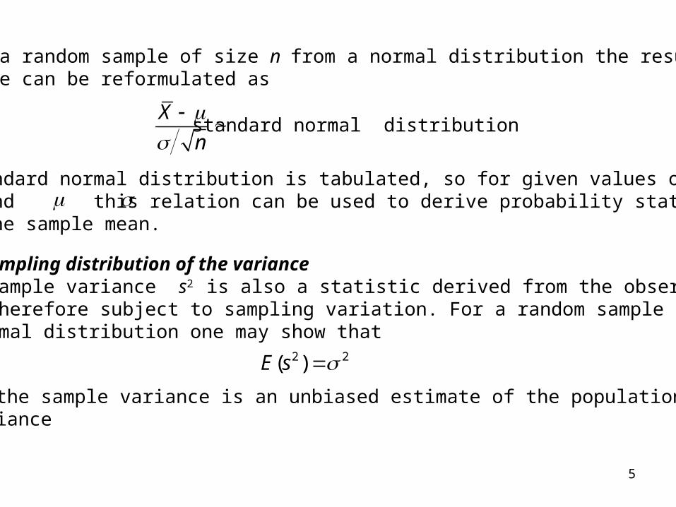
For a random sample of size n from a normal distribution the resultabove can be reformulated as
X
n
standard normal distribution
The standard normal distribution is tabulated, so for given values of and this relation can be used to derive probability statementsabout the sample mean.
The sampling distribution of the varianceThe sample variance s2 is also a statistic derived from the observationsand therefore subject to sampling variation. For a random sample froma normal distribution one may show that
2 2( )E s
so the sample variance is an unbiased estimate of the population variance
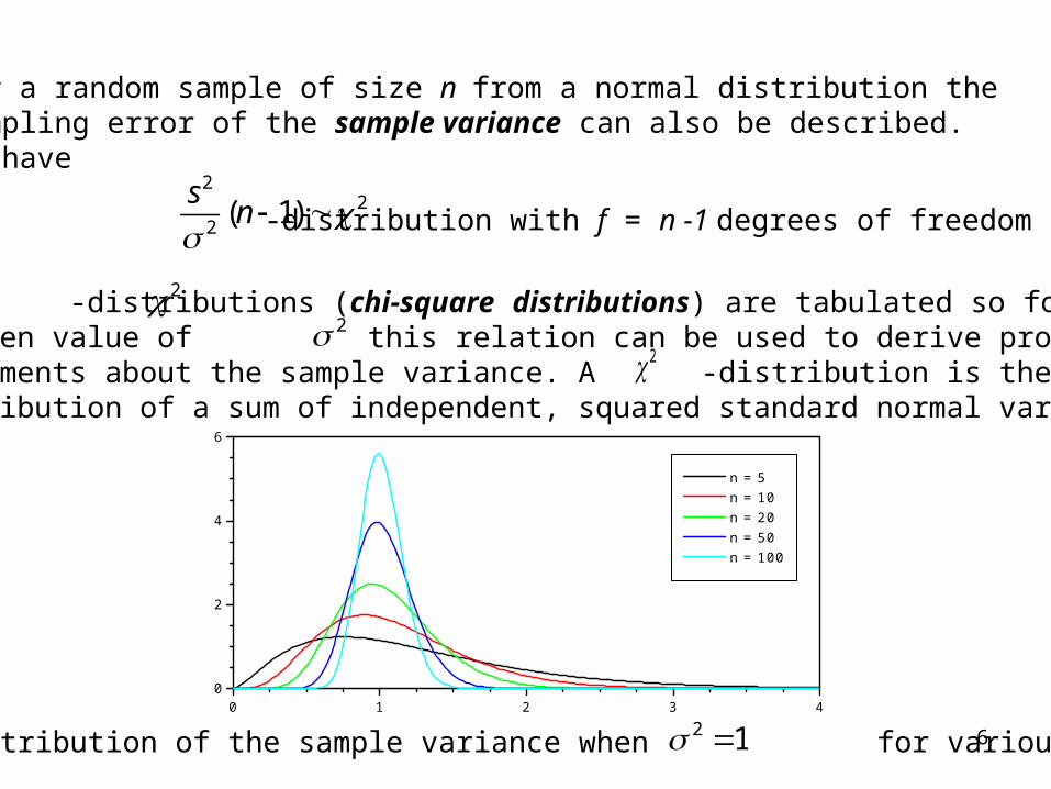
6The distribution of the sample variance when for various n. 0 1 2 3 4
0
2
4
6
n = 5 n = 10 n = 20 n = 50 n = 100
For a random sample of size n from a normal distribution the sampling error of the sample variance can also be described.We have
22
2( 1)
sn
-distribution with f = n -1 degrees of freedom
The -distributions (chi-square distributions) are tabulated so fora given value of this relation can be used to derive probabilitystatements about the sample variance. A -distribution is the distribution of a sum of independent, squared standard normal variates.
22
2 1
2
7
INTRODUCTION TO STATISTICAL INFERENCE
Statistical inference: The use of a statistical analysis of data to draw conclusions from observations subject to random variation.
Data are considered as a sample from a population (real or hypothetical)The purpose of the statistical analysis is to make statements about certain aspects of this population
The basic components of a statistical analysis• Specification of a relevant statistical model (the scientific problem
is ”translated” to a statistical problem)• Estimation of the population characteristics (the model parameters)• Validation of the underlying assumptions• Test of hypotheses about the model parameters.
A statistical analysis is always based on a statistical model, which formalizes the assumptions made about the sampling procedure and the random and systematic variation in the population from which the sample is drawn.
8
The validity of the conclusions depends on the degree to which the statistical model gives an adequate description of the sampling procedure and the random and systematic variation.
Consequently, checking the appropriateness of the underlying assumptions (i.e. the statistical model) is an important part of a statistical analysis.
The statistical model should be seen as an approximation to the real world.
The choice of a suitable model is always a balance between
complex models, which are close approximations, but very difficult to use in practice,
andsimple models, which are crude approximations, but easy to apply
9
Example: Comparing the efficacy of two treatments
Design: Experimental units (e.g. patients) are allocated to two treatments. For each experimental unit in both treatment groups an outcome is measured. The outcome reflects the efficacy of the treatment.
Purpose: To compare the efficacy of the two treatments
Analysis: To summarize the results the average outcome is computed in each group and the two averages are compared.
Possible explanations for a discrepancy between the average outcome in the two groups
• The treatments have different efficacy. One is better than the other
• Random variation
• Bias originating from other differences between the groups. Other factors which influence the outcome may differ between the groups and lead to apparent differences between the efficacy of the twotreatments (confounding).
10
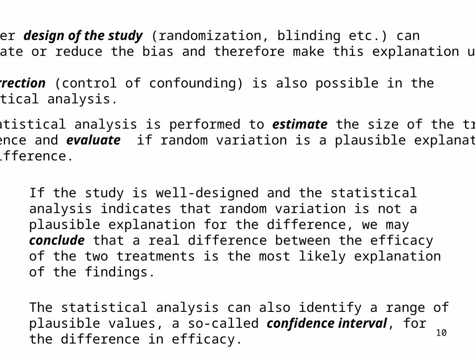
A proper design of the study (randomization, blinding etc.) can eliminate or reduce the bias and therefore make this explanation unlikely.
Bias correction (control of confounding) is also possible in the statistical analysis.
The statistical analysis is performed to estimate the size of the treatmentdifference and evaluate if random variation is a plausible explanation for this difference.
If the study is well-designed and the statistical analysis indicates that random variation is not a plausible explanation for the difference, we may conclude that a real difference between the efficacy of the two treatments is the most likely explanation of the findings.
The statistical analysis can also identify a range of plausible values, a so-called confidence interval, for the difference in efficacy.
11
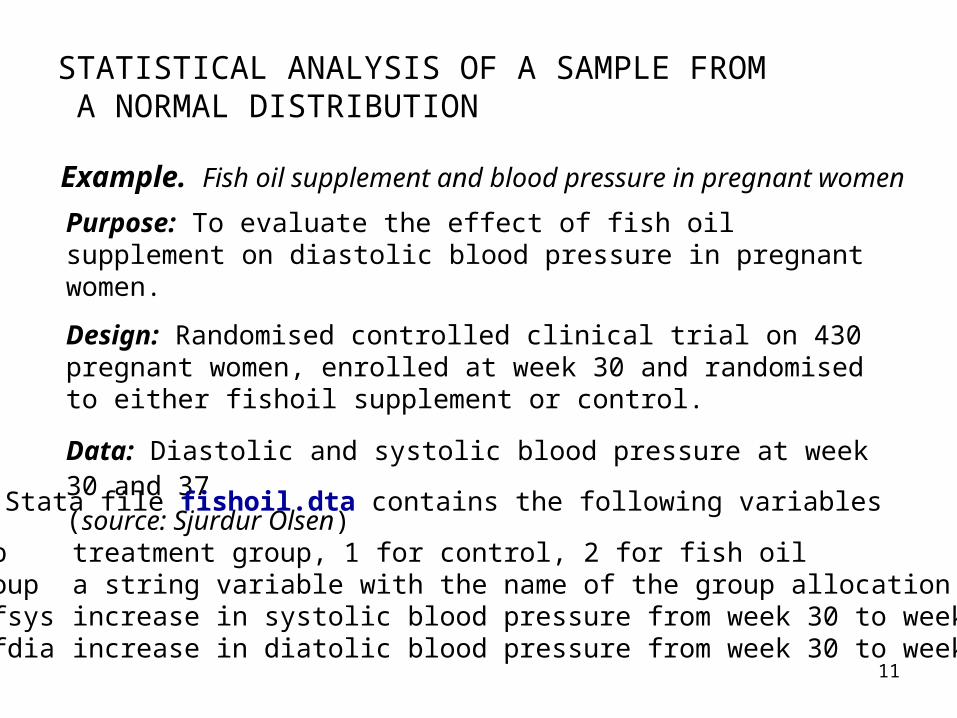
STATISTICAL ANALYSIS OF A SAMPLE FROM A NORMAL DISTRIBUTION
Example. Fish oil supplement and blood pressure in pregnant women
Purpose: To evaluate the effect of fish oil supplement on diastolic blood pressure in pregnant women.
Design: Randomised controlled clinical trial on 430 pregnant women, enrolled at week 30 and randomised to either fishoil supplement or control.
Data: Diastolic and systolic blood pressure at week 30 and 37 (source: Sjurdur Olsen)
The Stata file fishoil.dta contains the following variables
grp treatment group, 1 for control, 2 for fish oilgroup a string variable with the name of the group allocationdifsys increase in systolic blood pressure from week 30 to week 37difdia increase in diatolic blood pressure from week 30 to week 37
12
0
.02
.04
.06
-40 -20 0 20 40 -40 -20 0 20 40
Control Fishoil
De
nsi
ty
difdiaGraphs by group
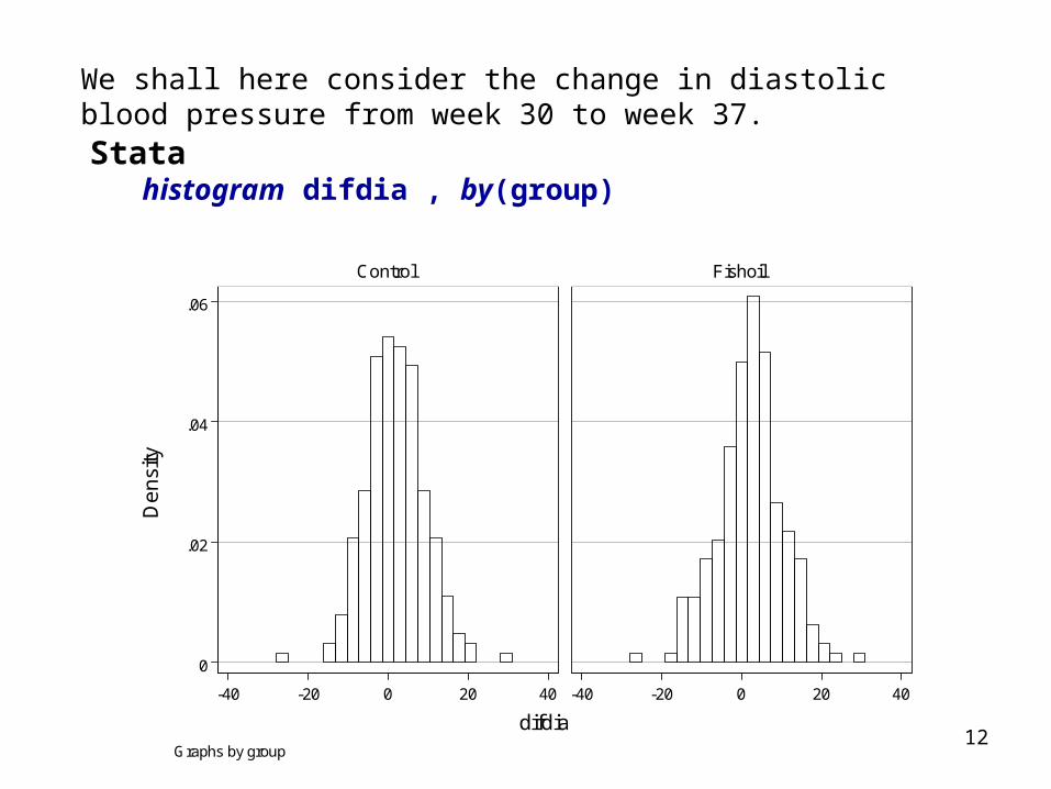
We shall here consider the change in diastolic blood pressure from week 30 to week 37. Stata
histogram difdia , by(group)
13
-40
-20
0
20
40
difd
ia
-20 -10 0 10 20
Inverse Normal
Control
-40
-20
0
20
40
difd
ia
-20 -10 0 10 20
Inverse Normal
Fish oil
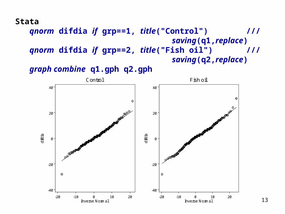
Stataqnorm difdia if grp==1, title("Control") ///
saving(q1,replace)qnorm difdia if grp==2, title("Fish oil") ///
saving(q2,replace)graph combine q1.gph q2.gph
14
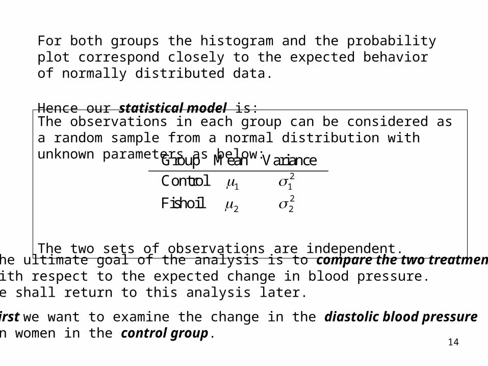
For both groups the histogram and the probability plot correspond closely to the expected behavior of normally distributed data.
Hence our statistical model is:
The observations in each group can be considered as a random sample from a normal distribution with unknown parameters as below:
The two sets of observations are independent.
21 1
22 2
Group Mean Variance Control
Fishoil
The ultimate goal of the analysis is to compare the two treatments with respect to the expected change in blood pressure. We shall return to this analysis later.
First we want to examine the change in the diastolic blood pressure in women in the control group.
15
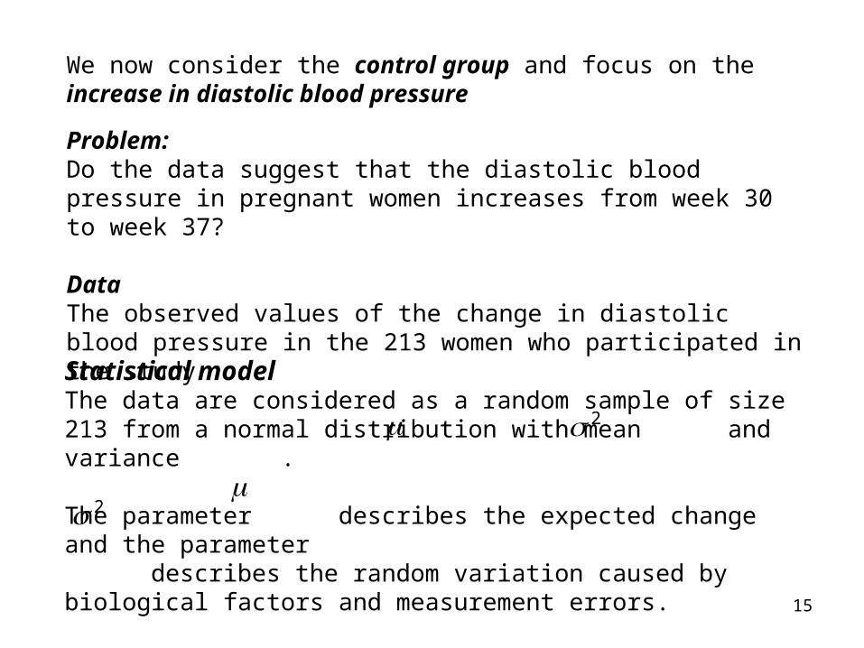
We now consider the control group and focus on the increase in diastolic blood pressure
Statistical modelThe data are considered as a random sample of size 213 from a normal distribution with mean and variance .
The parameter describes the expected change and the parameter describes the random variation caused by biological factors and measurement errors.
2
2
Problem: Do the data suggest that the diastolic blood pressure in pregnant women increases from week 30 to week 37?
DataThe observed values of the change in diastolic blood pressure in the 213 women who participated in the study
16
AssumptionsThe assumptions of the statistical model are
1. The observations are independent
2. The observations have the same mean and the same variance
3. A normal distribution describes the variation.
Checking the validity of the assumptions is usually done by various plots and diagrams. Knowledge of the measurement process can often help in identifying points which need special attention.
Re 1. Checking independence often involves going through the sampling procedure. Here the assumption would e.g. be violated if the same woman contributes with more than one pregnancy.
Re 2. Do we have “independent replications of the same experiment”? Factors that are known to be associated with changes in blood pressure are not accounted for in the model. They contribute to the random variation.
17
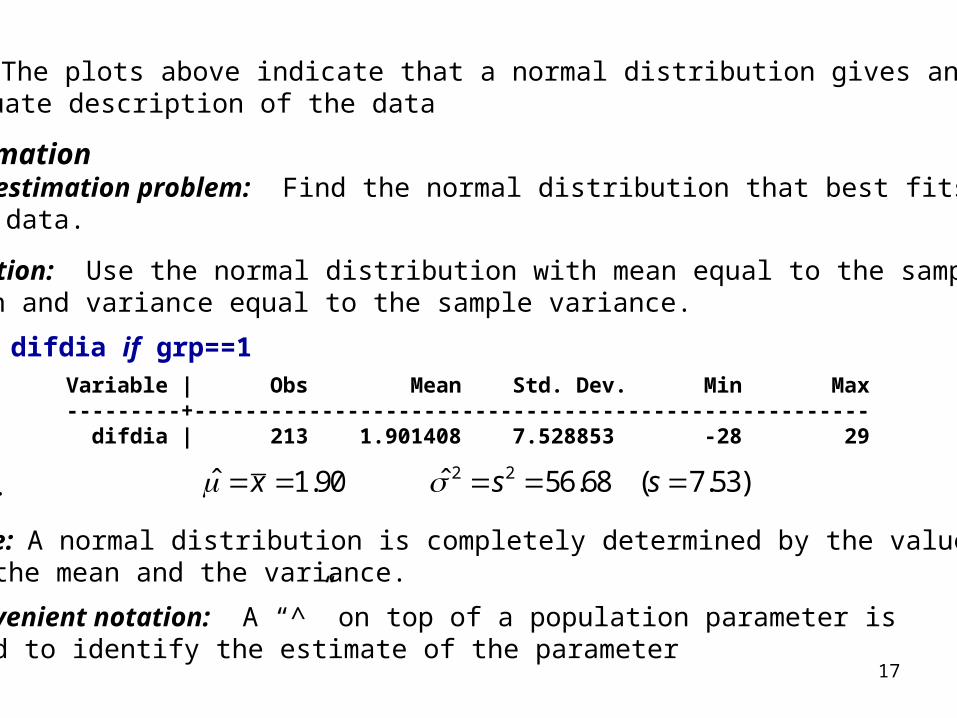
Re 3. The plots above indicate that a normal distribution gives an adequate description of the data
EstimationThe estimation problem: Find the normal distribution that best fits the data.
Solution: Use the normal distribution with mean equal to the sample mean and variance equal to the sample variance.
sum difdia if grp==1Variable | Obs Mean Std. Dev. Min Max---------+----------------------------------------------------- difdia | 213 1.901408 7.528853 -28 29
i.e.
Note: A normal distribution is completely determined by the values of the mean and the variance.
Convenient notation: A “^” on top of a population parameter is used to identify the estimate of the parameter
2 2ˆ ˆ1.90 56.68 ( 7.53)x s s
18
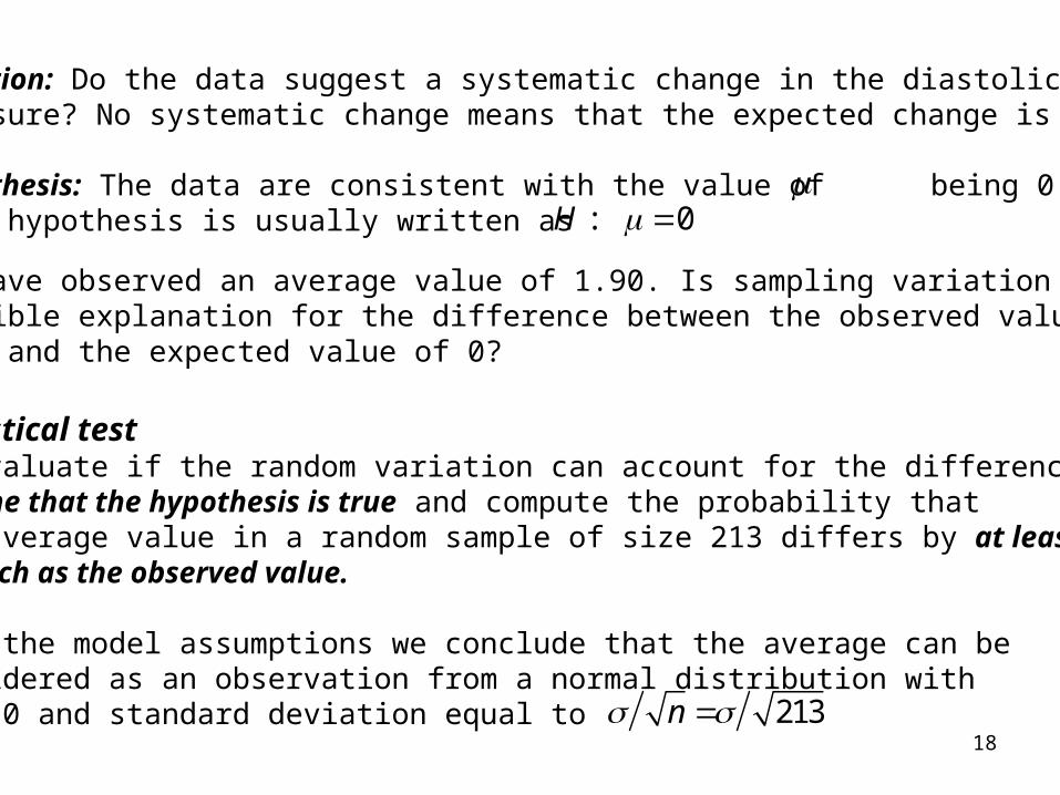
Question: Do the data suggest a systematic change in the diastolic pressure? No systematic change means that the expected change is 0, i.e.Hypothesis: The data are consistent with the value of being 0. This hypothesis is usually written as
We have observed an average value of 1.90. Is sampling variation a possible explanation for the difference between the observed value of 1.90 and the expected value of 0?
: 0H
Statistical testTo evaluate if the random variation can account for the difference we assume that the hypothesis is true and compute the probability that the average value in a random sample of size 213 differs by at least as much as the observed value.
From the model assumptions we conclude that the average can be considered as an observation from a normal distribution with mean 0 and standard deviation equal to 213n
19
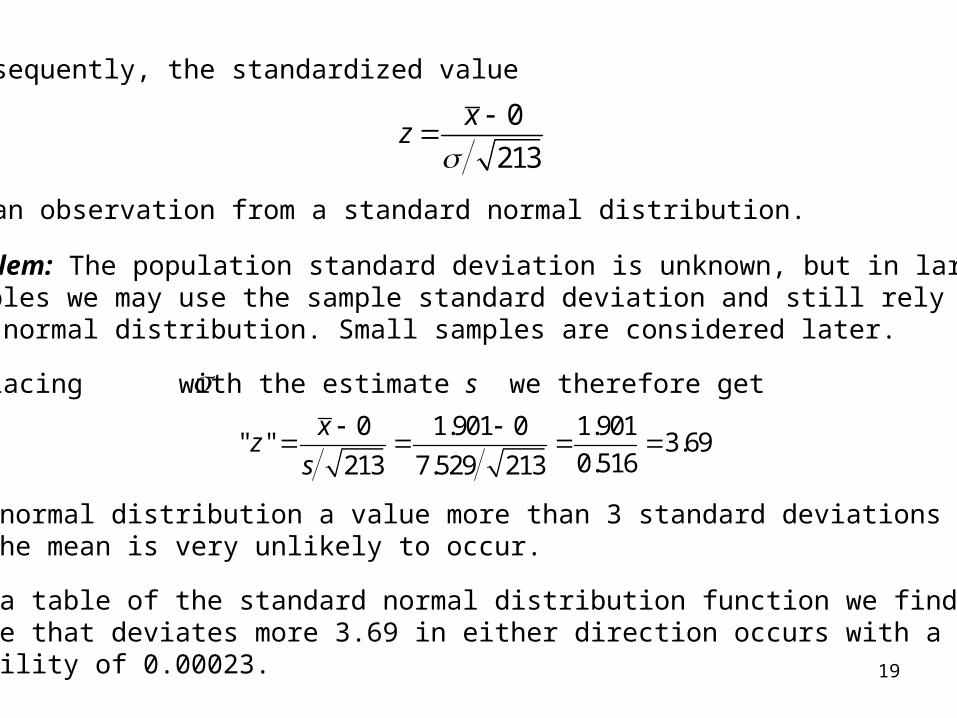
Consequently, the standardized value
is an observation from a standard normal distribution.
0
213
xz
Problem: The population standard deviation is unknown, but in large samples we may use the sample standard deviation and still rely on the normal distribution. Small samples are considered later.
Replacing with the estimate s we therefore get0 1.901 0 1.901
" " 3.690.516213 7.529 213
xz
s
For a normal distribution a value more than 3 standard deviations from the mean is very unlikely to occur.
Using a table of the standard normal distribution function we find thata value that deviates more 3.69 in either direction occurs with a probability of 0.00023.
20
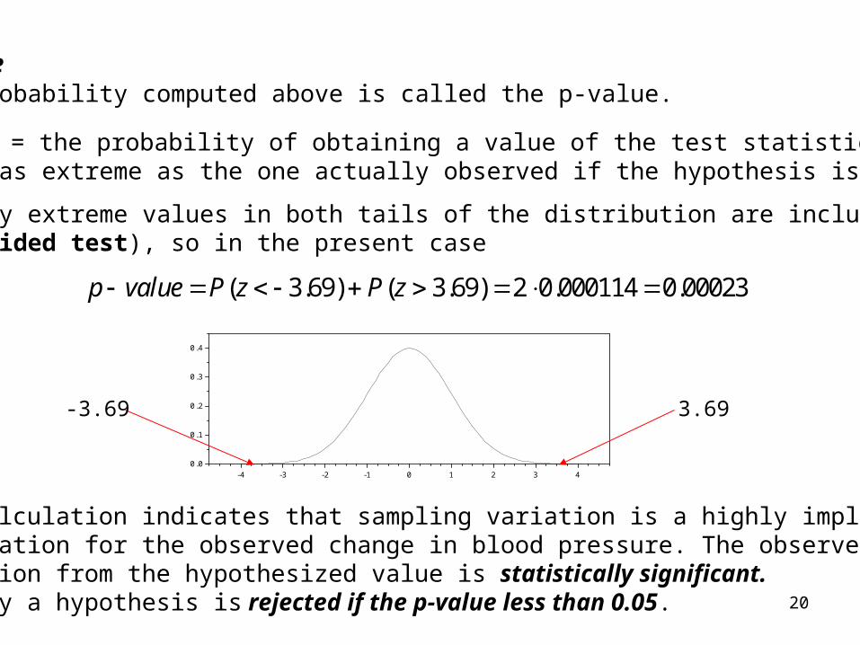
p-valueThe probability computed above is called the p-value.
p-value = the probability of obtaining a value of the test statistics asleast as extreme as the one actually observed if the hypothesis is true.
Usually extreme values in both tails of the distribution are included (two-sided test), so in the present case
( 3.69) ( 3.69) 2 0.000114 0.00023p value P z P z
-4 -3 -2 -1 0 1 2 3 40.0
0.1
0.2
0.3
0.4
The calculation indicates that sampling variation is a highly implausible explanation for the observed change in blood pressure. The observed deviation from the hypothesized value is statistically significant. Usually a hypothesis is rejected if the p-value less than 0.05.
3.69-3.69
21
SMALL SAMPLES – use of the t – distribution
The t-distribution has been tabulated, so we are still able to computea p-value. Note that the t-distributions does not depend on the parameters and so the same table applies in all situations.
As the sample size increases the t-distribution will approach a standardnormal distribution. Usually the approximation is acceptable for sampleslarger than 60, say.
2
To compute the p-value above we replaced the unknown population standard deviation with the sample standard deviation and referred the value of the test statistic to a normal distribution.
For large samples this approach is unproblematic, but for small samples the p-value becomes too small, since the sampling error of the sample standard deviation is ignored. Statistical theory shows that the correctdistribution of the test statistic is a so-called t-distribution with f = n – 1 degrees of freedom.
22
-4 -2 0 2 40.0
0.1
0.2
0.3
0.4
standard normal t-dist. n = 5 t-dist. n = 20 t-dist. n = 100
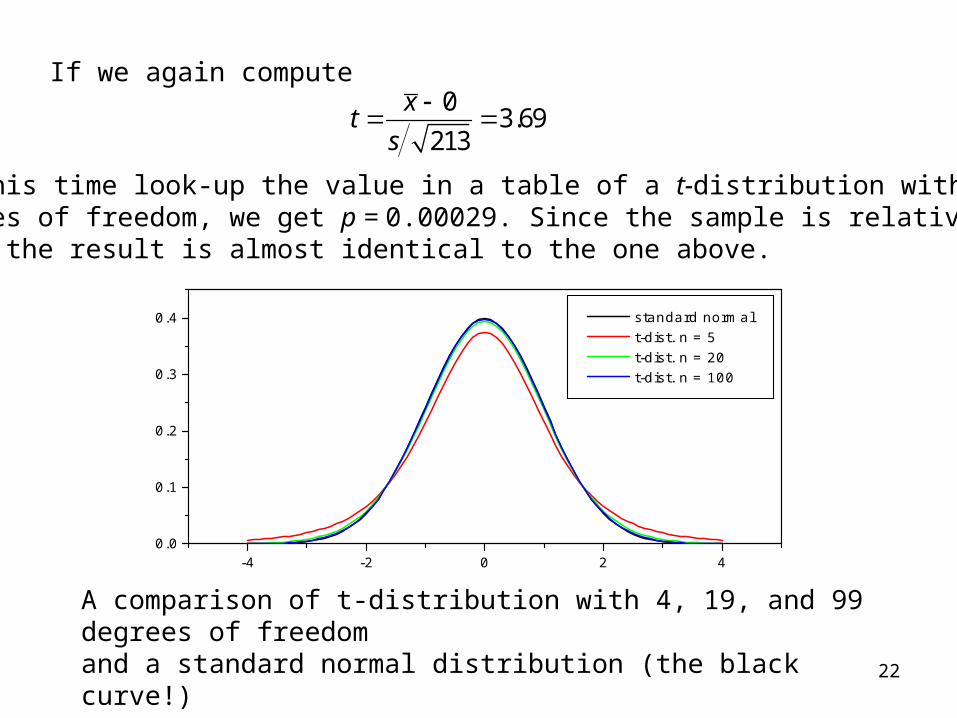
If we again compute 0
3.69213
xts
but this time look-up the value in a table of a t-distribution with f = 212 degrees of freedom, we get p = 0.00029. Since the sample is relativelylarge the result is almost identical to the one above.
A comparison of t-distribution with 4, 19, and 99 degrees of freedomand a standard normal distribution (the black curve!)
23
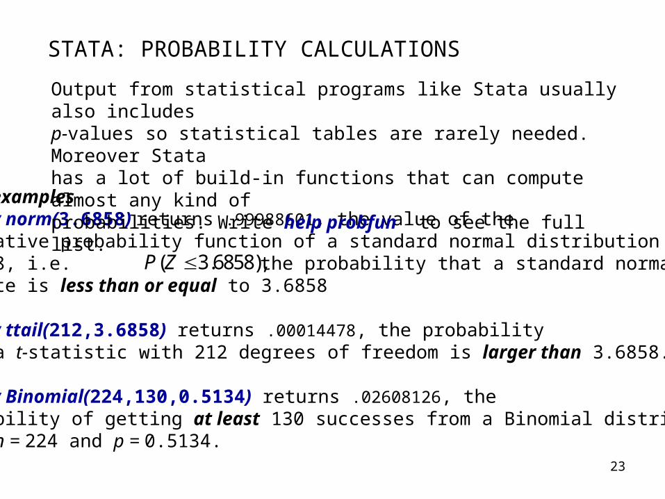
STATA: PROBABILITY CALCULATIONS
Some examplesdisplay norm(3.6858) returns .99988601, the value of the cumulative probability function of a standard normal distribution at3.6858, i.e. the probability that a standard normal variate is less than or equal to 3.6858
display ttail(212,3.6858) returns .00014478, the probability that a t-statistic with 212 degrees of freedom is larger than 3.6858.
display Binomial(224,130,0.5134) returns .02608126, the probability of getting at least 130 successes from a Binomial distribution with n = 224 and p = 0.5134.
( 3.6858),P Z
Output from statistical programs like Stata usually also includes p-values so statistical tables are rarely needed. Moreover Statahas a lot of build-in functions that can compute almost any kind of probabilities. Write help probfun to see the full list.
24
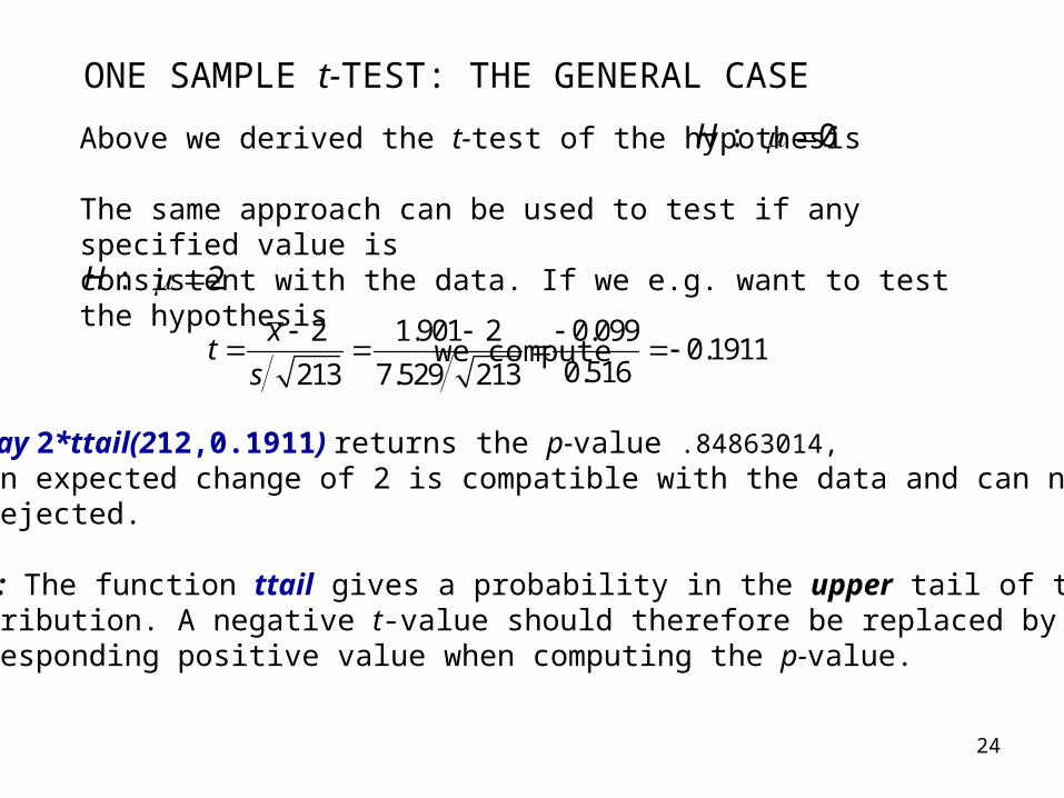
ONE SAMPLE t-TEST: THE GENERAL CASE
Above we derived the t-test of the hypothesis
The same approach can be used to test if any specified value isconsistent with the data. If we e.g. want to test the hypothesis we compute
: 0H
: 2H
2 1.901 2 0.0990.1911
0.516213 7.529 213
xts
display 2*ttail(212,0.1911) returns the p-value .84863014, so an expected change of 2 is compatible with the data and can not be rejected.
Note: The function ttail gives a probability in the upper tail of thedistribution. A negative t-value should therefore be replaced by the corresponding positive value when computing the p-value.
25
CONFIDENCE INTERVALS
In the example the observed average change in blood pressure is 1.901, and this value was used as an estimate of the expected change
Values close to 1.901 are also compatible with the data, we saw e.g.that the value 2 could not be rejected.
Problem: Find the range of values for the expected change that is supported by the data.
A confidence interval is the solution to this problem.
Formally: A 95% confidence interval identifies the values of the unknown parameter which would not be significantly contradicted by a (two-sided) test at the 5% level, because the p-value associated with the test statistic for each of these values is larger than 5%
26
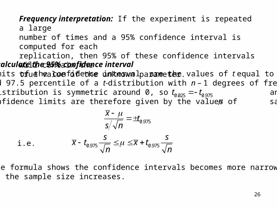
Frequency interpretation: If the experiment is repeated a large number of times and a 95% confidence interval is computed for eachreplication, then 95% of these confidence intervals will contain thetrue value of the unknown parameter.
How to calculate the 95% confidence intervalThe limits of the confidence interval are the values of t equal to the2.5 and 97.5 percentile of a t-distribution with n – 1 degrees of freedom.The t-distribution is symmetric around 0, so and the the confidence limits are therefore given by the values of satisfying
0.025 0.975t t
0.975
xt
s n
i.e. 0.975 0.975
s sx t x t
n n
The formula shows the confidence intervals becomes more narrowas the sample size increases.
27
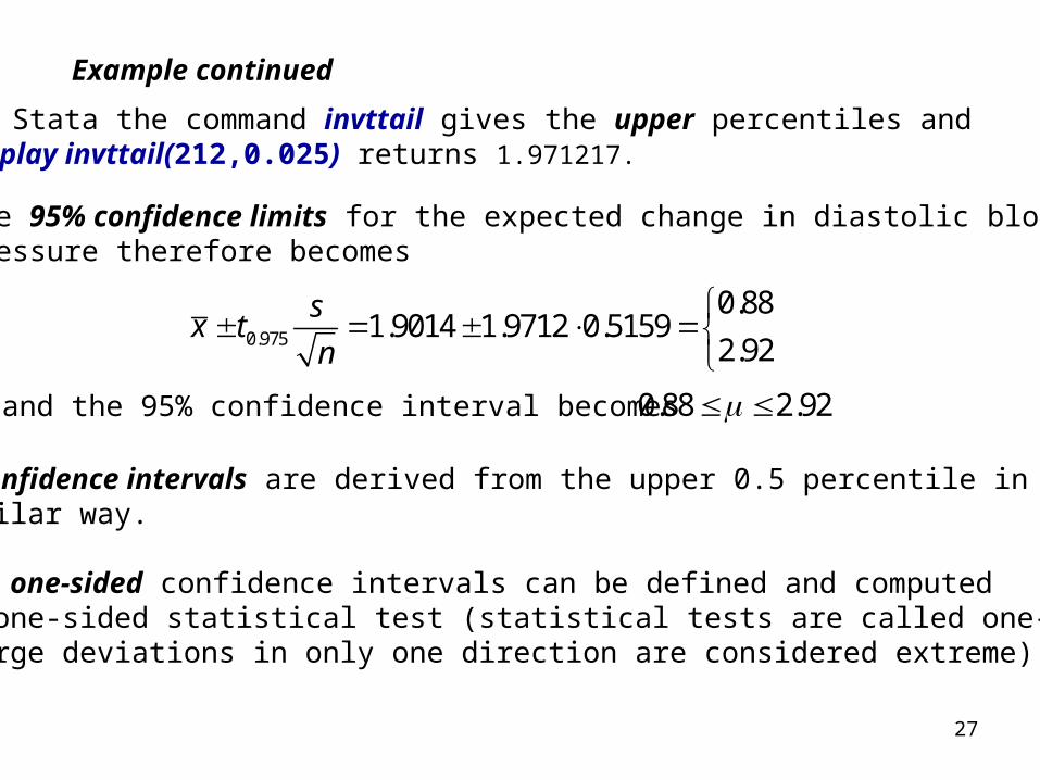
Example continued
0.975
0.881.9014 1.9712 0.5159
2.92
sx t
n
0.88 2.92 and the 95% confidence interval becomes
In Stata the command invttail gives the upper percentiles anddisplay invttail(212,0.025) returns 1.971217.
The 95% confidence limits for the expected change in diastolic blood pressure therefore becomes
99% confidence intervals are derived from the upper 0.5 percentile ina similar way.
Also, one-sided confidence intervals can be defined and computedfrom one-sided statistical test (statistical tests are called one-sided if large deviations in only one direction are considered extreme).
28
STATA: ONE SAMPLE t-TEST
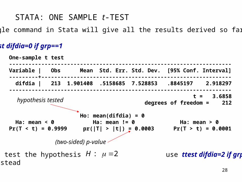
A single command in Stata will give all the results derived so far.
ttest difdia=0 if grp==1
One-sample t test---------------------------------------------------------------------Variable | Obs Mean Std. Err. Std. Dev. [95% Conf. Interval]---------+----------------------------------------------------------- difdia | 213 1.901408 .5158685 7.528853 .8845197 2.918297--------------------------------------------------------------------- t = 3.6858 degrees of freedom = 212
Ho: mean(difdia) = 0 Ha: mean < 0 Ha: mean != 0 Ha: mean > 0Pr(T < t) = 0.9999 pr(|T| > |t|) = 0.0003 Pr(T > t) = 0.0001
To test the hypothesis use ttest difdia=2 if grp==1instead
: 2H
(two-sided) p-value
hypothesis tested
29
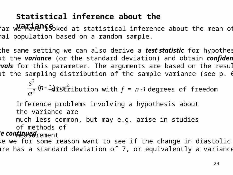
Statistical inference about the variance
So far we have looked at statistical inference about the mean of a normal population based on a random sample.
In the same setting we can also derive a test statistic for hypothesesabout the variance (or the standard deviation) and obtain confidenceintervals for this parameter. The arguments are based on the resultabout the sampling distribution of the sample variance (see p. 6)
22
2( 1)
sn
-distribution with f = n -1 degrees of freedom
Example continuedSuppose we for some reason want to see if the change in diastolic bloodpressure has a standard deviation of 7, or equivalently a variance of 49.
Inference problems involving a hypothesis about the variance aremuch less common, but may e.g. arise in studies of methods of measurement
30
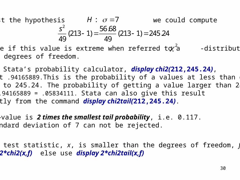
To test the hypothesis we could compute : 7H 2 56.68
(213 1) (213 1) 245.2449 49
s
and see if this value is extreme when referred to a -distributionon 212 degrees of freedom.
2
Using Stata’s probability calculator, display chi2(212,245.24), we get .94165889.This is the probability of a values at less than or equal to 245.24. The probability of getting a value larger than 245.24 is 1-.94165889 = .05834111. Stata can also give this result directly from the command display chi2tail(212,245.24).
The p-value is 2 times the smallest tail probability, i.e. 0.117. A standard deviation of 7 can not be rejected.
Rule: If the test statistic, x, is smaller than the degrees of freedom, f, use display 2*chi2(x,f) else use display 2*chi2tail(x,f)
31
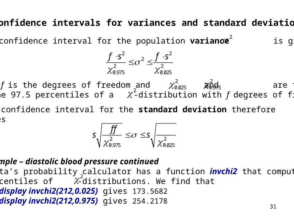
Confidence intervals for variances and standard deviations
A 95% confidence interval for the population variance is given by 2
2 22
2 20.975 0.025
f s f s
where f is the degrees of freedom and and are the 2.5and the 97.5 percentiles of a -distribution with f degrees of freedom.
A 95% confidence interval for the standard deviation therefore becomes
20.025 2
0.9752
2 20.975 0.025
f fs s
Example – diastolic blood pressure continuedStata’s probability calculator has a function invchi2 that computespercentiles of -distributions. We find that
display invchi2(212,0.025) gives 173.5682display invchi2(212,0.975) gives 254.2178
2
32
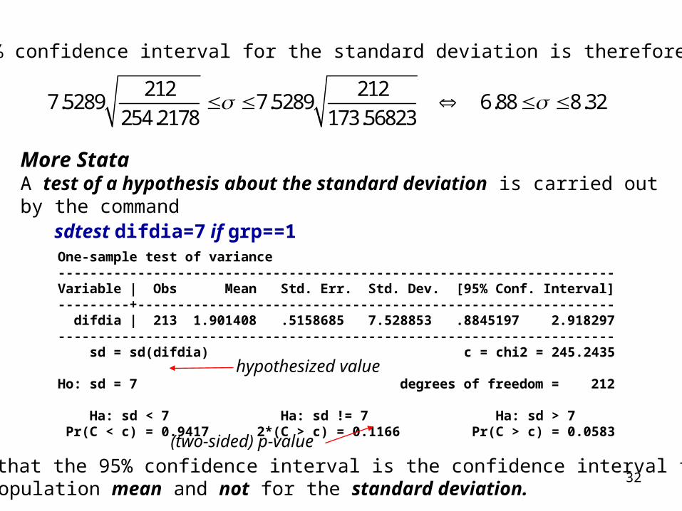
A 95% confidence interval for the standard deviation is therefore
212 2127.5289 7.5289 6.88 8.32
254.2178 173.56823
More StataA test of a hypothesis about the standard deviation is carried outby the command
sdtest difdia=7 if grp==1One-sample test of variance----------------------------------------------------------------------Variable | Obs Mean Std. Err. Std. Dev. [95% Conf. Interval]---------+------------------------------------------------------------ difdia | 213 1.901408 .5158685 7.528853 .8845197 2.918297---------------------------------------------------------------------- sd = sd(difdia) c = chi2 = 245.2435 Ho: sd = 7 degrees of freedom = 212 Ha: sd < 7 Ha: sd != 7 Ha: sd > 7 Pr(C < c) = 0.9417 2*(C > c) = 0.1166 Pr(C > c) = 0.0583
Note that the 95% confidence interval is the confidence interval for the population mean and not for the standard deviation.
hypothesized value
(two-sided) p-value
33
STATISTICAL ANALYSIS OF TWO INDEPENDENT SAMPLES FROM NORMAL DISTRIBUTIONS
Example. Fish oil supplement and blood pressure in pregnant women
The study was a randomized trial carried out to evaluate the effect of fishoil supplement on diastolic blood pressure in pregnant women.
Pregnant women were assigned at random to one of two treatment groups. One group received fish oil supplement, the other was acontrol group.
Here we shall compare the two treatments using difdia, the change in diastolic blood pressure, as outcome, or response.
We have already seen histograms and Q-Q plots of the distribution of difdia in each of the two groups (see p. 12-13) and these plotssuggest that the random variation may be adequately described by normal distributions.
34
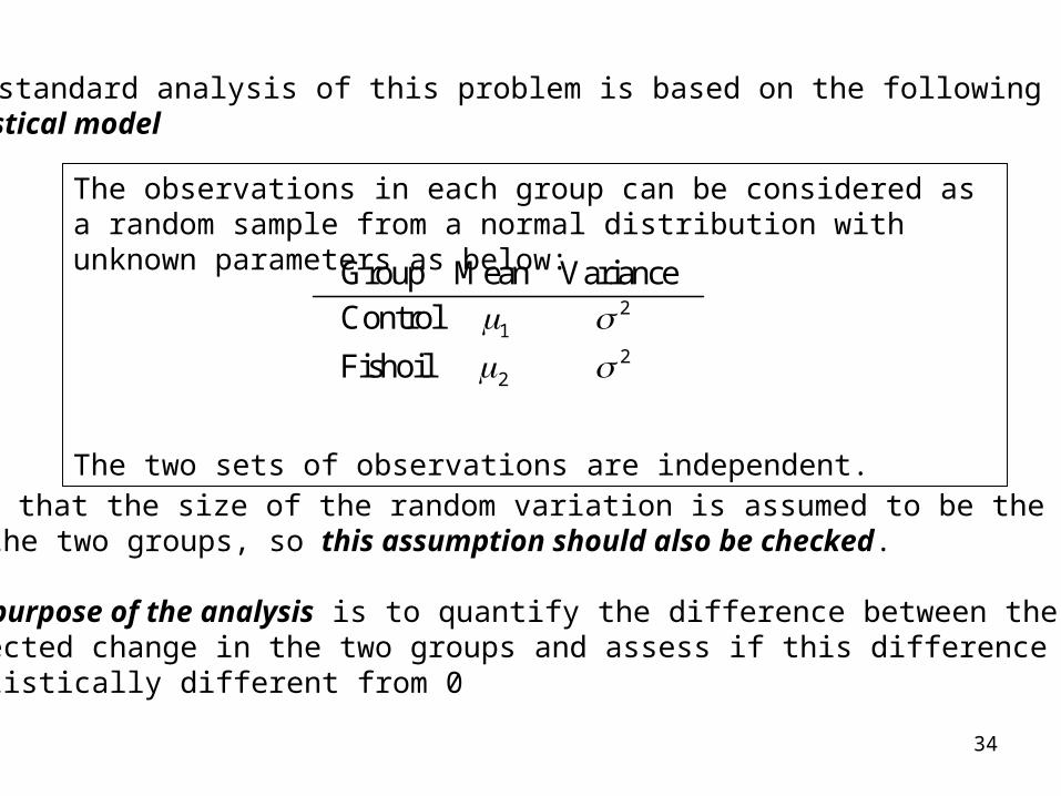
The observations in each group can be considered as a random sample from a normal distribution with unknown parameters as below:
The two sets of observations are independent.
21
22
Group Mean Variance Control
Fishoil
The standard analysis of this problem is based on the followingstatistical model
Note that the size of the random variation is assumed to be the samein the two groups, so this assumption should also be checked.
The purpose of the analysis is to quantify the difference between the expected change in the two groups and assess if this difference is statistically different from 0
35
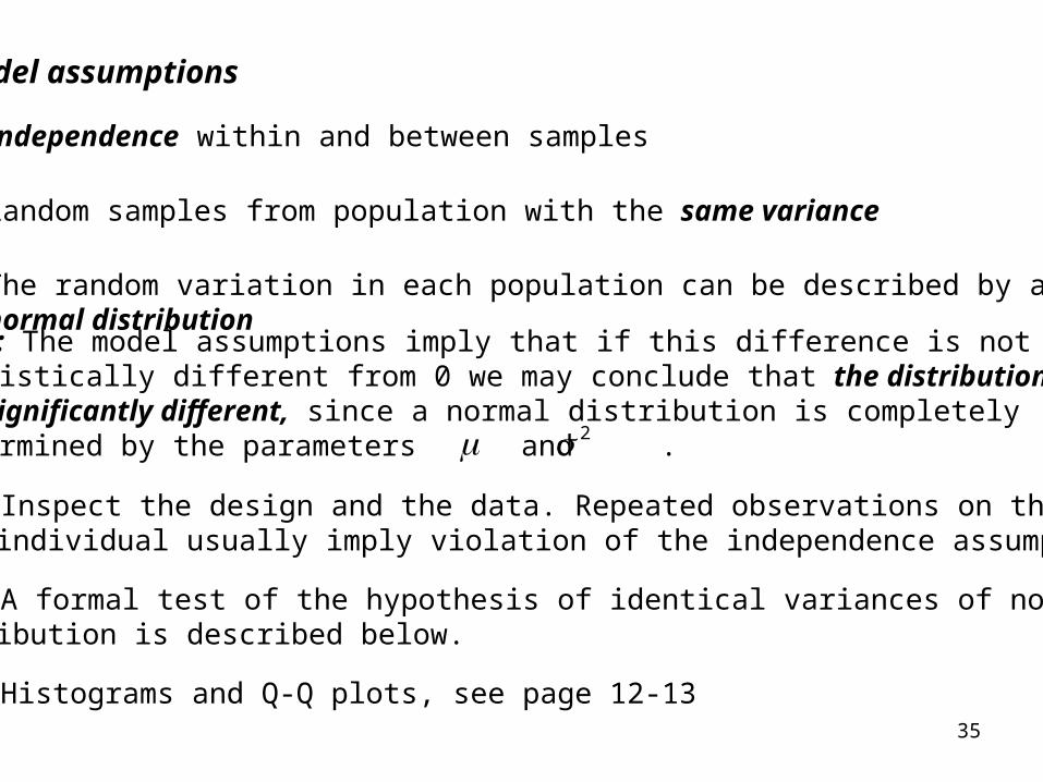
Note: The model assumptions imply that if this difference is not statistically different from 0 we may conclude that the distributions arenot significantly different, since a normal distribution is completelydetermined by the parameters and . 2
Model assumptions
1. Independence within and between samples
2. Random samples from population with the same variance
3. The random variation in each population can be described by anormal distribution
Re 1. Inspect the design and the data. Repeated observations on the same individual usually imply violation of the independence assumption.
Re 2. A formal test of the hypothesis of identical variances of normaldistribution is described below.
Re 3. Histograms and Q-Q plots, see page 12-13
36
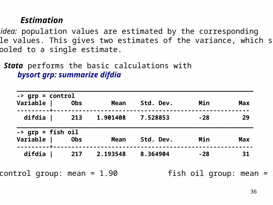
EstimationBasic idea: population values are estimated by the correspondingsample values. This gives two estimates of the variance, which shouldbe pooled to a single estimate.
Stata performs the basic calculations withbysort grp: summarize difdia
_________________________________________________________________-> grp = controlVariable | Obs Mean Std. Dev. Min Max---------+------------------------------------------------------ difdia | 213 1.901408 7.528853 -28 29_________________________________________________________________-> grp = fish oilVariable | Obs Mean Std. Dev. Min Max---------+------------------------------------------------------- difdia | 217 2.193548 8.364904 -28 31
i.e. control group: mean = 1.90 fish oil group: mean = 2.19
37
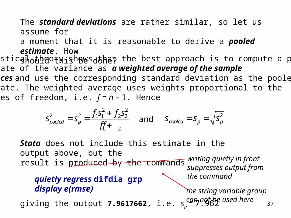
Stata does not include this estimate in the output above, but the result is produced by the commands
quietly regress difdia grpdisplay e(rmse)
giving the output 7.9617662, i.e. sp = 7.962
Statistical theory shows that the best approach is to compute a pooled estimate of the variance as a weighted average of the sample variances and use the corresponding standard deviation as the pooled estimate. The weighted average uses weights proportional to the degrees of freedom, i.e. f = n – 1. Hence
2 22 2 1 1 2 2
1 2pooled p
f s f ss s
f f
and
2pooled p ps s s
writing quietly in frontsuppresses output from the command
the string variable groupcan not be used here
The standard deviations are rather similar, so let us assume for a moment that it is reasonable to derive a pooled estimate. Howshould this be done?
38
Statistical test comparing means of two independent samplesThe expected change in diastolic blood pressure is slightly higher in the fish oil group. Does this reflect a systematic effect?
To see if random variation can explain the difference we test the hypothesis
1 2:H
of identical population means in the two samples.
The line of argument is similar to the one that was used in the one-sample case. Assume that the hypothesis is true. This observeddifference between the two means must then be caused by samplingvariation.
The plausibility of this explanation is assessed by computing a p-value,the probability of obtaining a result at least as extreme as the observed.
39
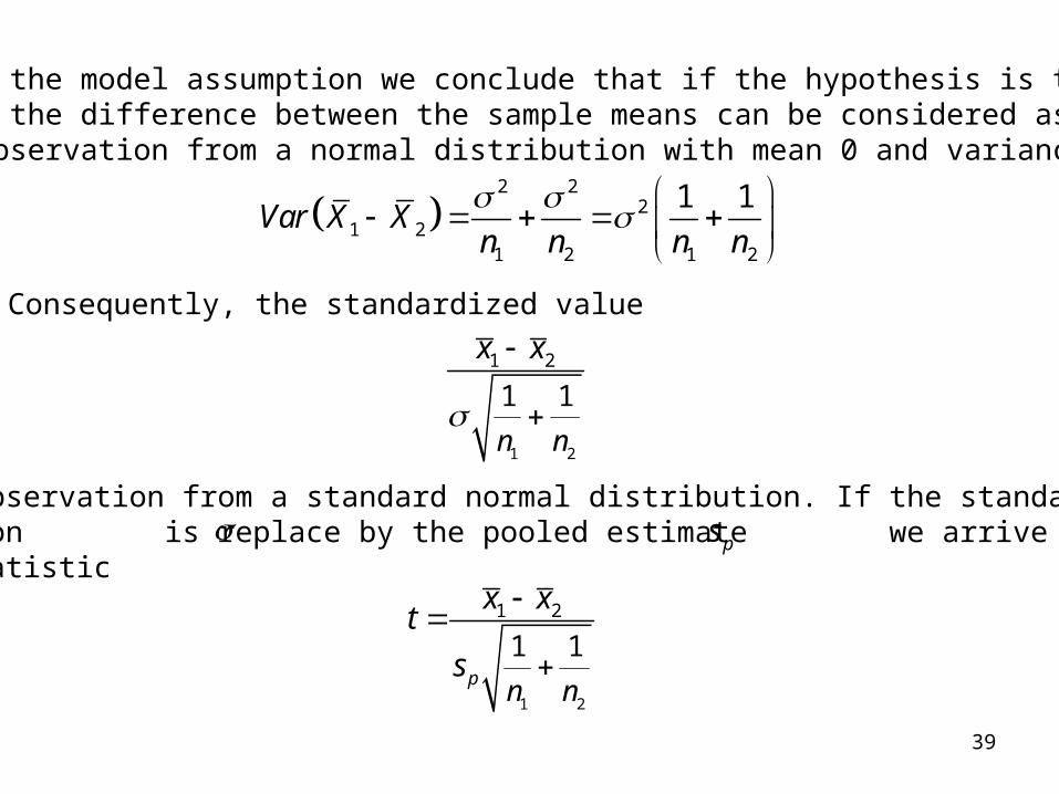
From the model assumption we conclude that if the hypothesis is truethen the difference between the sample means can be considered asan observation from a normal distribution with mean 0 and variance
2 2
21 2
1 2 1 2
1 1Var X X
n n n n
Consequently, the standardized value
1 2
1 2
1 1
n n
x x
is an observation from a standard normal distribution. If the standarddeviation is replace by the pooled estimate we arrive at thetest statistic
1 2
1 2
1 1pn n
x xt
s
ps
40
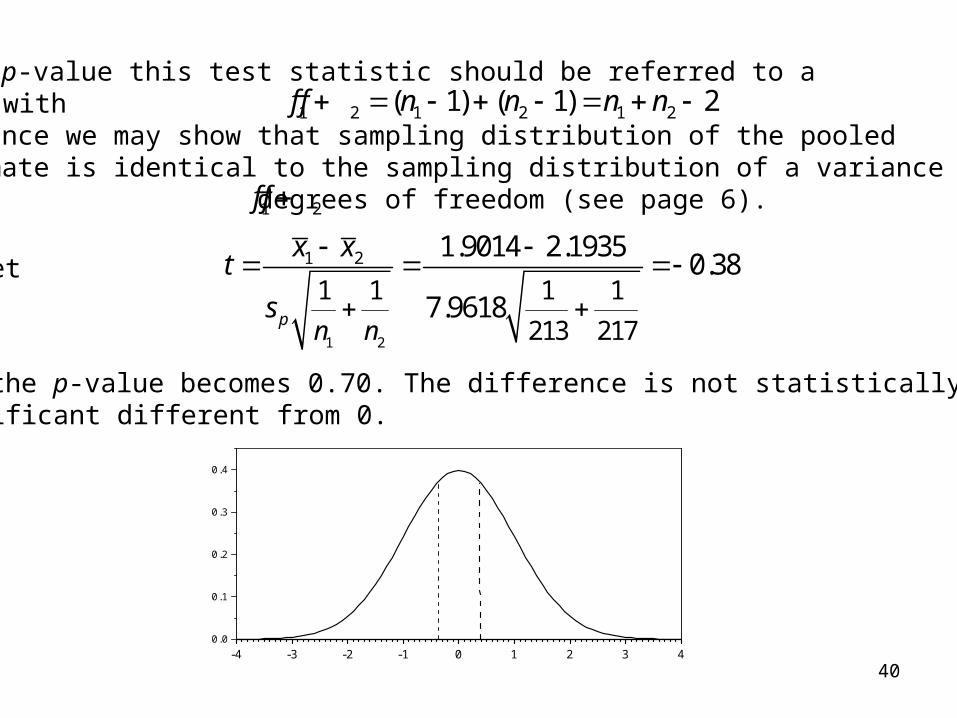
To derive the p-value this test statistic should be referred to a t-distribution with degrees of freedom, since we may show that sampling distribution of the pooledvariance estimate is identical to the sampling distribution of a variance estimate with degrees of freedom (see page 6).
1 2 1 2 1 2( 1) ( 1) 2f f n n n n
1 2f f
We get
and the p-value becomes 0.70. The difference is not statistically significant different from 0.
1 2
1 2
1 1 1 1
213 217
1.9014 2.19350.38
7.9618pn n
x xt
s
-4 -3 -2 -1 0 1 2 3 40.0
0.1
0.2
0.3
0.4
41
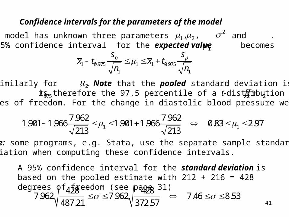
Confidence intervals for the parameters of the model
The model has unknown three parameters and . A 95% confidence interval for the expected value becomes 1
1 0.975 1 1 0.975
1 1
p ps sx t x t
n n
and similarly for . Note that the pooled standard deviation is usedand is therefore the 97.5 percentile of a t-distribution with degrees of freedom. For the change in diastolic blood pressure we get
2.975t 1 2f f
1 1
7.962 7.9621.901 1.966 1.901 1.966 0.83 2.97
213 213
Note: some programs, e.g. Stata, use the separate sample standarddeviation when computing these confidence intervals.
A 95% confidence interval for the standard deviation is based on the pooled estimate with 212 + 216 = 428 degrees of freedom (see page 31)
428 4287.962 7.962 7.46 8.53
487.21 372.57
1 2, , 2
42
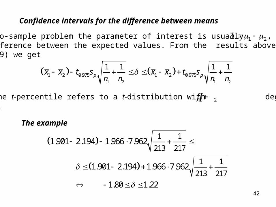
Confidence intervals for the difference between means
In a two-sample problem the parameter of interest is usually the difference between the expected values. From the results above(page 39) we get
1 2 ,
1 2 1 2
1 2 0.975 1 2 0.975
1 1 1 1p pn n n n
x x t s x x t s
where the t-percentile refers to a t-distribution with degrees of freedom.
1 2f f
The example
1 1
213 217
1 1
213 217
1.901 2.194 1.966 7.962
1.901 2.194 1.966 7.962
1.80 1.22
43
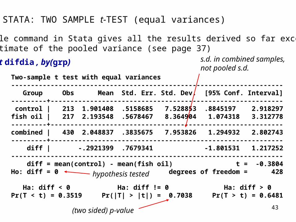
Two-sample t test with equal variances--------------------------------------------------------------------- Group Obs Mean Std. Err. Std. Dev. [95% Conf. Interval]---------+----------------------------------------------------------- control | 213 1.901408 .5158685 7.528853 .8845197 2.918297fish oil | 217 2.193548 .5678467 8.364904 1.074318 3.312778---------+-----------------------------------------------------------combined | 430 2.048837 .3835675 7.953826 1.294932 2.802743---------+----------------------------------------------------------- diff | -.2921399 .7679341 -1.801531 1.217252--------------------------------------------------------------------- diff = mean(control) - mean(fish oil) t = -0.3804 Ho: diff = 0 degrees of freedom = 428
Ha: diff < 0 Ha: diff != 0 Ha: diff > 0 Pr(T < t) = 0.3519 Pr(|T| > |t|) = 0.7038 Pr(T > t) = 0.6481
STATA: TWO SAMPLE t-TEST (equal variances)
A single command in Stata gives all the results derived so far exceptand estimate of the pooled variance (see page 37)
ttest difdia , by(grp)
hypothesis tested
(two sided) p-value
s.d. in combined samples,not pooled s.d.
44
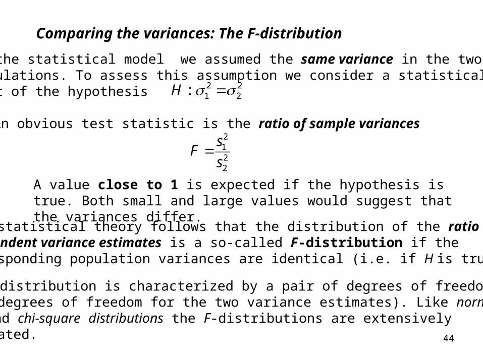
Comparing the variances: The F-distribution
In the statistical model we assumed the same variance in the two populations. To assess this assumption we consider a statistical test of the hypothesis
2 21 2:H
An obvious test statistic is the ratio of sample variances2122
sF
s
A value close to 1 is expected if the hypothesis is true. Both small and large values would suggest that the variances differ.
From statistical theory follows that the distribution of the ratio of twoindependent variance estimates is a so-called F-distribution if the corresponding population variances are identical (i.e. if H is true).
The F-distribution is characterized by a pair of degrees of freedom (the degrees of freedom for the two variance estimates). Like normal, t-, and chi-square distributions the F-distributions are extensively tabulated.
45
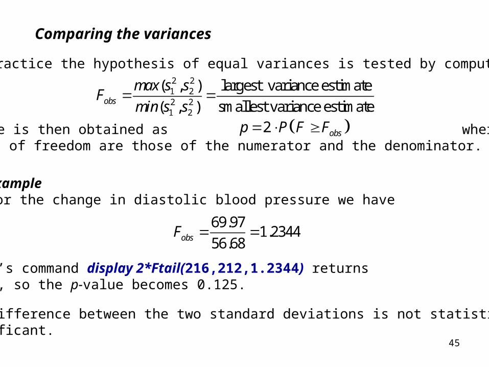
Comparing the variances
In practice the hypothesis of equal variances is tested by computing2 21 22 21 2
( , ) largest variance estimate
( , ) smallest variance estimateobs
max s sF
min s s
and p-value is then obtained as where the pair of degrees of freedom are those of the numerator and the denominator.
2 obsp P F F
ExampleFor the change in diastolic blood pressure we have
69.971.2344
56.68obsF
Stata’s command display 2*Ftail(216,212,1.2344) returns 0.125, so the p-value becomes 0.125.
The difference between the two standard deviations is not statisticallysignificant.
46
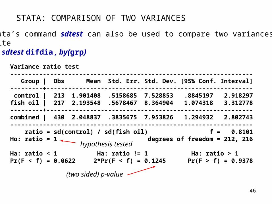
Variance ratio test------------------------------------------------------------------- Group | Obs Mean Std. Err. Std. Dev. [95% Conf. Interval]---------+--------------------------------------------------------- control | 213 1.901408 .5158685 7.528853 .8845197 2.918297fish oil | 217 2.193548 .5678467 8.364904 1.074318 3.312778---------+---------------------------------------------------------combined | 430 2.048837 .3835675 7.953826 1.294932 2.802743------------------------------------------------------------------- ratio = sd(control) / sd(fish oil) f = 0.8101Ho: ratio = 1 degrees of freedom = 212, 216
Ha: ratio < 1 Ha: ratio != 1 Ha: ratio > 1Pr(F < f) = 0.0622 2*Pr(F < f) = 0.1245 Pr(F > f) = 0.9378
(two sided) p-value
hypothesis tested
STATA: COMPARISON OF TWO VARIANCES
Stata’s command sdtest can also be used to compare two variances.Write
sdtest difdia , by(grp)
47
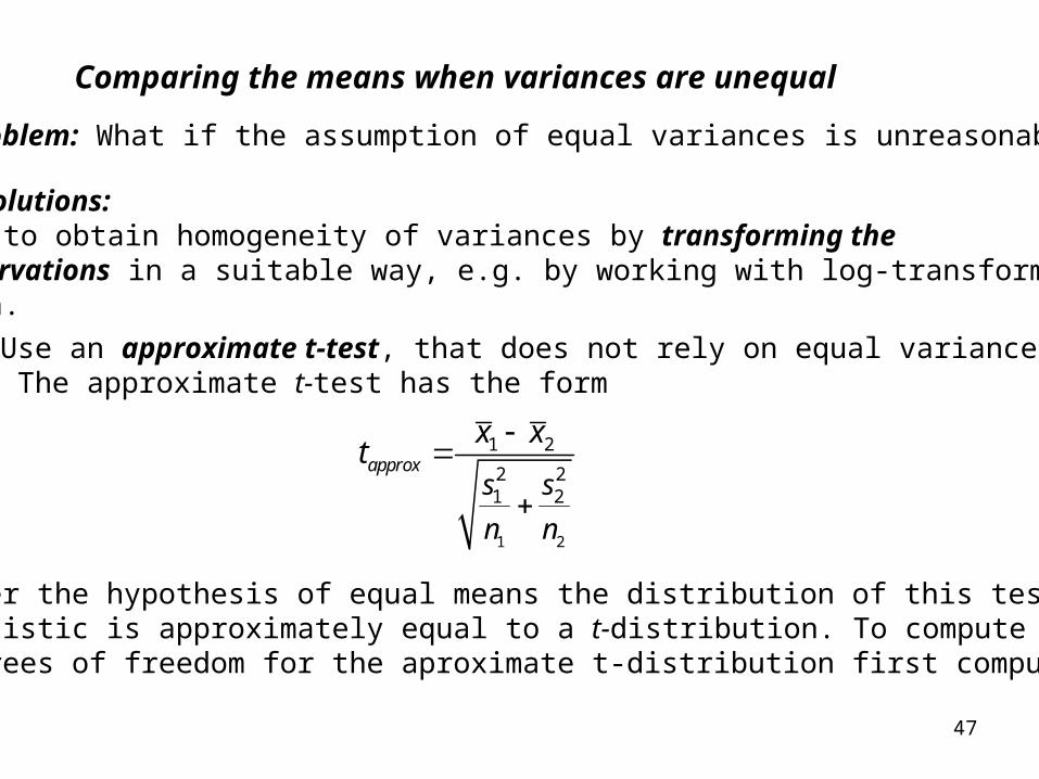
Comparing the means when variances are unequal
Problem: What if the assumption of equal variances is unreasonable?
Some solutions:1. Try to obtain homogeneity of variances by transforming the
observations in a suitable way, e.g. by working with log-transformed data.
1 2
1 2
2 21 2
approxs s
n n
x xt
Under the hypothesis of equal means the distribution of this test statistic is approximately equal to a t-distribution. To compute the degrees of freedom for the aproximate t-distribution first compute
2. Use an approximate t-test, that does not rely on equal variances. The approximate t-test has the form
48
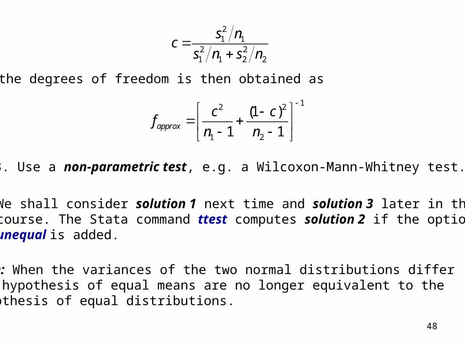
21 1
2 21 1 2 2
s ncs n s n
the degrees of freedom is then obtained as
12 2
1 2
(1 )
1 1approx
c cf
n n
3. Use a non-parametric test, e.g. a Wilcoxon-Mann-Whitney test.
We shall consider solution 1 next time and solution 3 later in thecourse. The Stata command ttest computes solution 2 if the optionunequal is added.
Note: When the variances of the two normal distributions differ the hypothesis of equal means are no longer equivalent to the hypothesis of equal distributions.
49
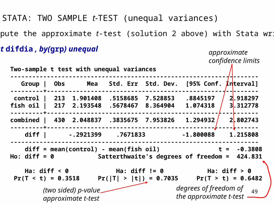
Two-sample t test with unequal variances-------------------------------------------------------------------- Group | Obs Mea Std. Err Std. Dev. [95% Conf. Interval]---------+---------------------------------------------------------- control | 213 1.901408 .5158685 7.528853 .8845197 2.918297fish oil | 217 2.193548 .5678467 8.364904 1.074318 3.312778---------+----------------------------------------------------------combined | 430 2.048837 .3835675 7.953826 1.294932 2.802743---------+---------------------------------------------------------- diff | -.2921399 .7671833 -1.800088 1.215808-------------------------------------------------------------------- diff = mean(control) - mean(fish oil) t = -0.3808Ho: diff = 0 Satterthwaite's degrees of freedom = 424.831
Ha: diff < 0 Ha: diff != 0 Ha: diff > 0 Pr(T < t) = 0.3518 Pr(|T| > |t|) = 0.7035 Pr(T > t) = 0.6482
STATA: TWO SAMPLE t-TEST (unequal variances)
To compute the approximate t-test (solution 2 above) with Stata write
ttest difdia , by(grp) unequal
(two sided) p-valueapproximate t-test
degrees of freedom ofthe approximate t-test
approximateconfidence limits
50
SOME GENERAL COMMENTS ON STATISTICAL TESTS
To test a hypothesis we compute a test statistic, which follows a known distribution if the hypothesis is true. We can therefore computethe probability of obtaining a value of the test statistic as least as extreme as the one observed. This probability is called the p-value.
The p-value describes the degrees of support of the hypothesis foundin the data. The result of the statistical test is often classified as ”statistical significant” or ”non-significant” depending on whether ornot the p-value is smaller than a level of significance, often called ,and usually equal to 0.05.
Hypothesis testing is sometimes given a decision theoretic formulation:The null hypothesis is either true or false and a decision is made basedon the data.
The hypothesis being tested is often called the null hypothesis. A null hypothesis always represents a simplication of the statistical model.
51
When hypothesis testing is viewed as decisions, two types of error arepossible
• Type 1 error: Rejecting a true null hypothesis• Type 2 error: Accepting (i.e. not rejecting) a false null hypothesis.
The level of significance specifies the risk of a type 1 error. In theusual setting the null hypothesis is tested against an alternative hypothesis which includes different values of the parameter, e.g.
0 : 0 : 0 AH H against
The risk of a type 2 error depends on which of the alternative valuesare the true value.
The power of a statistical test is 1 minus the risk of type 2 error. Whenplanning an experiment power considerations are sometimes usedto determine the sample size. We return to this in the last lecture.
Once the data are collected confidence intervals are the appropriate way to summarize the uncertainty in the conclusions.
52
Relation between p-values and confidence intervals
In a two sample problem it is tempting to compare the 95% confidence intervals of the two means and conclude that the hypothesis is non-significant if the 95% confidence intervals overlap.
This is not correct.
Overlapping 95% confidence intervals does not imply that the difference is not significant on a 5% level. On the other hand, if the 95% confidence intervals do not overlap, the difference is statistical significant on a 5% level (actually, the p-value is 1% or smaller).
1 2
This may at first seem surprising, but it is a simple consequence of thefact that for independent samples the result
implies that( ) ( ) ( )Var x y Var x Var y
( ) ( ) ( )se x y se x se y
Recommended