June 22, 2006 Software Engineering Working Group Meeting 2
MotivationMotivation
Petascale system with 100K - 500K procTrend or One off?
LLNL: 128K proc IBM BG/LIBM Watson: 40K proc IBM BG/LSandia: 10K proc IBM RedStormORNL/NCCS: 5K proc Cray XT3
10K (end of summer) -> 20K (Nov 06) -> ?ANL: Large IBM BG/P system
We have prototypes for Petascale system!
Petascale system with 100K - 500K procTrend or One off?
LLNL: 128K proc IBM BG/LIBM Watson: 40K proc IBM BG/LSandia: 10K proc IBM RedStormORNL/NCCS: 5K proc Cray XT3
10K (end of summer) -> 20K (Nov 06) -> ?ANL: Large IBM BG/P system
We have prototypes for Petascale system!

June 22, 2006 Software Engineering Working Group Meeting 3
Motivation (con’t)Motivation (con’t)
Prototype Petascale Application?POP @ 0.1 degree
BGW 30K proc --> 7.9 years/wallclock dayRedStorm 8K proc--> 8.1 years/wallclock day
Can CCSM be a Petascale Application?Look at each component separately
Current scalability limitationsChanges necessary to enable execution on
large processor countsCheck scalability on BG/L

June 22, 2006 Software Engineering Working Group Meeting 4
Motivation (con’t)Motivation (con’t)
Why examine scalability on BG/L? Prototype for Petascale system Access to large processor counts
2K easily40K through Blue Gene Watson Days
Scalable architecture Limited memory:
256MB (VN)512MB (CO)
Dedicated resources gives reproducible timings Lessons translate to other systems [Cray XT3]
Why examine scalability on BG/L? Prototype for Petascale system Access to large processor counts
2K easily40K through Blue Gene Watson Days
Scalable architecture Limited memory:
256MB (VN)512MB (CO)
Dedicated resources gives reproducible timings Lessons translate to other systems [Cray XT3]
June 22, 2006 Software Engineering Working Group Meeting 5
Outline:Outline:
MotivationPOPCICECLMCAM + CouplerConclusions
MotivationPOPCICECLMCAM + CouplerConclusions

June 22, 2006 Software Engineering Working Group Meeting 6
Parallel Ocean Program (POP)
Parallel Ocean Program (POP)
Modified base POP 2.0 base codeReduce execution time/ improve scalabilityMinor changes (~9 files)
Rework barotropic solverImprove load-balancing (space-filling curve)Pilfered CICE boundary exchange [NEW]
Significant advances in performancePOP @ 1 degree
128 POWER4 processors --> 2.1xPOP @ 0.1 degree
30K BG/L processors --> 2x8K RedStorm processors --> 1.3x

June 22, 2006 Software Engineering Working Group Meeting 7
POP using 20x24 blocks (gx1v3)
POP using 20x24 blocks (gx1v3)
POP data structureFlexible block structureland ‘block’ eliminationSmall blocks
Better {load balanced, land block elimination}
Larger halo overhead
Larger blocksSmaller halo overheadLoad imbalancedNo land block elimination
POP data structureFlexible block structureland ‘block’ eliminationSmall blocks
Better {load balanced, land block elimination}
Larger halo overhead
Larger blocksSmaller halo overheadLoad imbalancedNo land block elimination

June 22, 2006 Software Engineering Working Group Meeting 8
Outline:Outline:
MotivationPOP
New Barotropic solverCICE boundary exchangeSpace-filling curves
CICECLMCAM + CouplerConclusions
MotivationPOP
New Barotropic solverCICE boundary exchangeSpace-filling curves
CICECLMCAM + CouplerConclusions

June 22, 2006 Software Engineering Working Group Meeting 9
Alternate Data StructureAlternate Data Structure
2D data structure Advantages
Regular stride-1 access
Compact form of stencil operator
Disadvantages Includes land points Problem specific data
structure
2D data structure Advantages
Regular stride-1 access
Compact form of stencil operator
Disadvantages Includes land points Problem specific data
structure
1D data structure Advantages
No more land points General data structure
Disadvantages Indirect addressing Larger stencil operator
1D data structure Advantages
No more land points General data structure
Disadvantages Indirect addressing Larger stencil operator

June 22, 2006 Software Engineering Working Group Meeting 10
Using 1D data structures in POP2 solver (serial)
Using 1D data structures in POP2 solver (serial)
Replace solvers.F90Execution time on cache
microprocessorsExamine two CG algorithms w/Diagonal
precondPCG2 ( 2 inner products)PCG1 ( 1 inner product) [D’Azevedo 93]
Grid: test [128x192 grid points]w/(16x16)
Replace solvers.F90Execution time on cache
microprocessorsExamine two CG algorithms w/Diagonal
precondPCG2 ( 2 inner products)PCG1 ( 1 inner product) [D’Azevedo 93]
Grid: test [128x192 grid points]w/(16x16)

June 22, 2006 Software Engineering Working Group Meeting 11
0
1
2
3
4
5
6
POWER4 1.3 Ghz
Compute Platform
seconds for 20 timesteps
PCG2+2D
PCG1+2D
PCG2+1D
PCG1+1D
0
1
2
3
4
5
6
POWER4 1.3 Ghz
Compute Platform
seconds for 20 timesteps
PCG2+2D
PCG1+2D
PCG2+1D
PCG1+1D
Serial execution time on IBM POWER4 (test)
Serial execution time on IBM POWER4 (test)
56% reduction in cost/iteration

June 22, 2006 Software Engineering Working Group Meeting 12
Using 1D data structure in POP2 solver (parallel)
Using 1D data structure in POP2 solver (parallel)
New parallel halo update Examine several CG algorithms w/Diagonal
precond PCG2 ( 2 inner products) PCG1 ( 1 inner product)
Existing solver/preconditioner technology: Hypre (LLNL)
http://www.llnl.gov/CASC/linear_solvers PCG solver Preconditioners:
Diagonal
New parallel halo update Examine several CG algorithms w/Diagonal
precond PCG2 ( 2 inner products) PCG1 ( 1 inner product)
Existing solver/preconditioner technology: Hypre (LLNL)
http://www.llnl.gov/CASC/linear_solvers PCG solver Preconditioners:
Diagonal

June 22, 2006 Software Engineering Working Group Meeting 13
Solver execution time for POP2 (20x24) on BG/L
(gx1v3)
Solver execution time for POP2 (20x24) on BG/L
(gx1v3)
0
5
10
15
20
25
30
35
40
64
# processors
Seconds for 200 timesteps
PCG2+2D
PCG1+2D
PCG2+1D
PCG1+1D
Hypre (PCG+Diag)
0
5
10
15
20
25
30
35
40
64
# processors
Seconds for 200 timesteps
PCG2+2D
PCG1+2D
PCG2+1D
PCG1+1D
Hypre (PCG+Diag)
48% cost/iteration
27% cost/iteration

June 22, 2006 Software Engineering Working Group Meeting 14
Outline:Outline:
MotivationPOP
New Barotropic solverCICE boundary exchangeSpace-filling curves
CICECLMCAM + CouplerConclusions
MotivationPOP
New Barotropic solverCICE boundary exchangeSpace-filling curves
CICECLMCAM + CouplerConclusions

June 22, 2006 Software Engineering Working Group Meeting 15
CICE boundary exchangeCICE boundary exchange
POP applies 2D boundary exchange to 3D vars.
3D-update 2-33% of total timeSpecialized 3D boundary exchange
Reduce message countIncrease message lengthReduces dependence on machine latency
Pilfer CICE 4.0 boundary exchangeCode Reuse! :-)
POP applies 2D boundary exchange to 3D vars.
3D-update 2-33% of total timeSpecialized 3D boundary exchange
Reduce message countIncrease message lengthReduces dependence on machine latency
Pilfer CICE 4.0 boundary exchangeCode Reuse! :-)

June 22, 2006 Software Engineering Working Group Meeting 16
Simulation rate of POP @ gx1v3 on IBM POWER4
Simulation rate of POP @ gx1v3 on IBM POWER4
0
5
10
15
20
25
30
16 32 64 80 128
# processors
Simulated years/wallclock day
20x24+SFC+NB (PCG1+1D)20x24+SFC (PCG1+1D)single block (PCG1+1D)single block (PCG1+2D)
0
5
10
15
20
25
30
16 32 64 80 128
# processors
Simulated years/wallclock day
20x24+SFC+NB (PCG1+1D)20x24+SFC (PCG1+1D)single block (PCG1+1D)single block (PCG1+2D)
ret
50% of time in solver

June 22, 2006 Software Engineering Working Group Meeting 17
Performance of POP@gx1v3
Performance of POP@gx1v3
Three code modifications1D data structureSpace-filling curvesCICE boundary exchange
Cumulative impact is hugeSeparately 10-20% eachTogether 2.1x on 128 processors
Small improvements add up!
Three code modifications1D data structureSpace-filling curvesCICE boundary exchange
Cumulative impact is hugeSeparately 10-20% eachTogether 2.1x on 128 processors
Small improvements add up!

June 22, 2006 Software Engineering Working Group Meeting 18
Outline:Outline:
MotivationPOP
New Barotropic solverCICE boundary exchangeSpace-filling curves
CICECLMCAM + CouplerConclusions
MotivationPOP
New Barotropic solverCICE boundary exchangeSpace-filling curves
CICECLMCAM + CouplerConclusions
June 22, 2006 Software Engineering Working Group Meeting 19
Partitioning with Space-filling Curves
Partitioning with Space-filling Curves
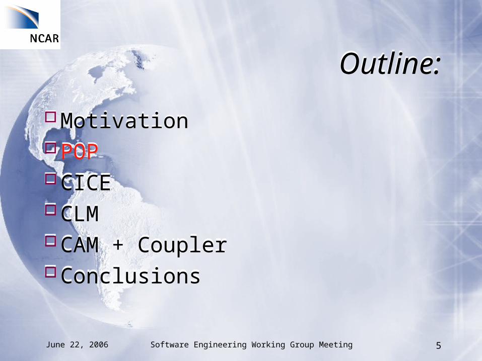
Map 2D -> 1DVariety of sizes
Hilbert (Nb=2n)
Peano (Nb=3m)
Cinco (Nb=5p) [New]Hilbert-Peano (Nb=2n3m)Hilbert-Peano-Cinco
(Nb=2n3m5p) [New]
Partitioning 1D array
Map 2D -> 1DVariety of sizes
Hilbert (Nb=2n)
Peano (Nb=3m)
Cinco (Nb=5p) [New]Hilbert-Peano (Nb=2n3m)Hilbert-Peano-Cinco
(Nb=2n3m5p) [New]
Partitioning 1D array
Nb

June 22, 2006 Software Engineering Working Group Meeting 20
Partitioning with SFCPartitioning with SFC
Partition for 3 processors

June 22, 2006 Software Engineering Working Group Meeting 21
POP using 20x24 blocks (gx1v3)
POP using 20x24 blocks (gx1v3)

June 22, 2006 Software Engineering Working Group Meeting 22
POP (gx1v3) + Space-filling curve
POP (gx1v3) + Space-filling curve

June 22, 2006 Software Engineering Working Group Meeting 23
Space-filling curve (Hilbert Nb=24)
Space-filling curve (Hilbert Nb=24)

June 22, 2006 Software Engineering Working Group Meeting 24
Remove Land blocksRemove Land blocks
June 22, 2006 Software Engineering Working Group Meeting 25
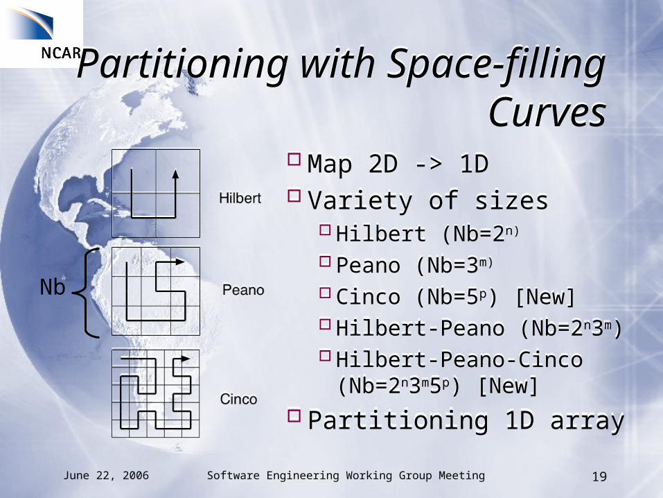
Space-filling curve partition for 8 processors
Space-filling curve partition for 8 processors

June 22, 2006 Software Engineering Working Group Meeting 26
0.1 degree POP0.1 degree POP
Global eddy-resolving Computational grid:
3600 x 2400 x 40Land creates problems:
load imbalancesscalability
Alternative partitioning algorithm:Space-filling curves
Evaluate using Benchmark:1 day/ Internal grid / 7 minute timestep
Global eddy-resolving Computational grid:
3600 x 2400 x 40Land creates problems:
load imbalancesscalability
Alternative partitioning algorithm:Space-filling curves
Evaluate using Benchmark:1 day/ Internal grid / 7 minute timestep

June 22, 2006 Software Engineering Working Group Meeting 27
POP 0.1 degree benchmark on Blue
Gene/L
POP 0.1 degree benchmark on Blue
Gene/L

June 22, 2006 Software Engineering Working Group Meeting 28
POP 0.1 degree benchmark
POP 0.1 degree benchmark
Courtesy of Y. Yoshida, M. Taylor, P. Worley
50% of time in solver
33% of time in 3D-update
June 22, 2006 Software Engineering Working Group Meeting 29
Remaining Issues: POPRemaining Issues: POP
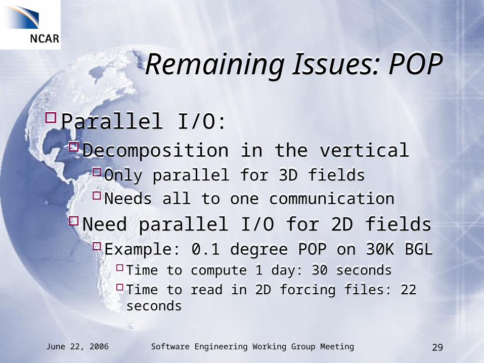
Parallel I/O:Decomposition in the vertical
Only parallel for 3D fieldsNeeds all to one communication
Need parallel I/O for 2D fieldsExample: 0.1 degree POP on 30K BGL
Time to compute 1 day: 30 secondsTime to read in 2D forcing files: 22 seconds
Parallel I/O:Decomposition in the vertical
Only parallel for 3D fieldsNeeds all to one communication
Need parallel I/O for 2D fieldsExample: 0.1 degree POP on 30K BGL
Time to compute 1 day: 30 secondsTime to read in 2D forcing files: 22 seconds
June 22, 2006 Software Engineering Working Group Meeting 30
Impact of 2x increase in simulation rate
Impact of 2x increase in simulation rate
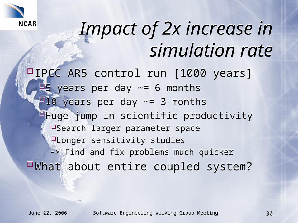
IPCC AR5 control run [1000 years]5 years per day ~= 6 months10 years per day ~= 3 monthsHuge jump in scientific productivity
Search larger parameter spaceLonger sensitivity studies-> Find and fix problems much quicker
What about entire coupled system?
IPCC AR5 control run [1000 years]5 years per day ~= 6 months10 years per day ~= 3 monthsHuge jump in scientific productivity
Search larger parameter spaceLonger sensitivity studies-> Find and fix problems much quicker
What about entire coupled system?
June 22, 2006 Software Engineering Working Group Meeting 31
Outline:Outline:
MotivationPOPCICECLMCAM + CouplerConclusions
MotivationPOPCICECLMCAM + CouplerConclusions

June 22, 2006 Software Engineering Working Group Meeting 32
CICE: Sea-ice ModelCICE: Sea-ice Model
Shares grid and infrastructure with POPCICE 4.0
Not quite ready for general releaseSub-block data structures (POP2)Minimal experience with code base
(<2 weeks)Reuse techniques from POP2 workPartitioning grid using weighted Space-
filling curves?
Shares grid and infrastructure with POPCICE 4.0
Not quite ready for general releaseSub-block data structures (POP2)Minimal experience with code base
(<2 weeks)Reuse techniques from POP2 workPartitioning grid using weighted Space-
filling curves?
June 22, 2006 Software Engineering Working Group Meeting 33
Weighted Space-filling curves
Weighted Space-filling curves
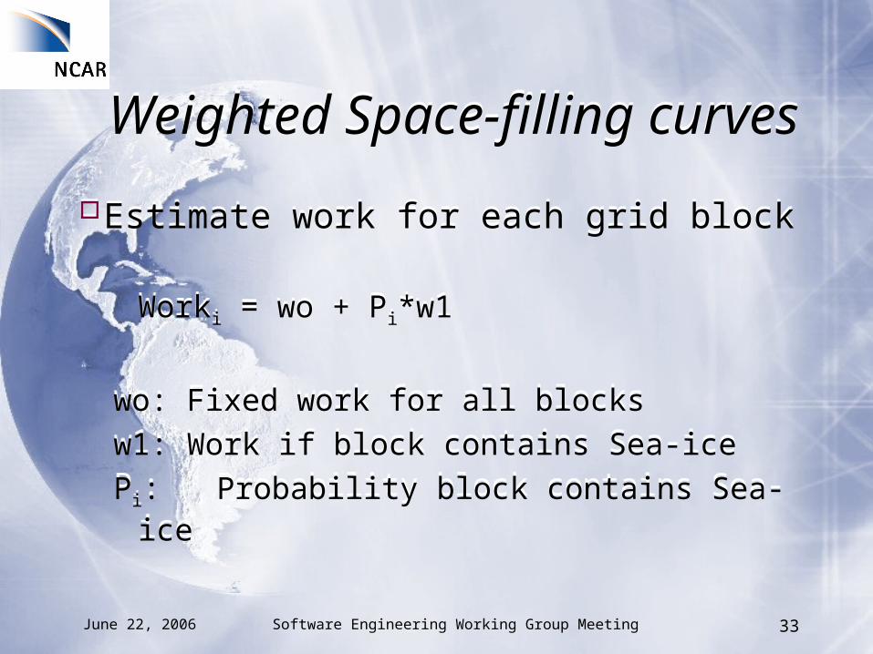
Estimate work for each grid block
Worki = wo + Pi*w1
wo: Fixed work for all blocksw1: Work if block contains Sea-icePi: Probability block contains Sea-
ice
Estimate work for each grid block
Worki = wo + Pi*w1
wo: Fixed work for all blocksw1: Work if block contains Sea-icePi: Probability block contains Sea-
ice

June 22, 2006 Software Engineering Working Group Meeting 34
Weighted Space-filling curves (con’t)
Weighted Space-filling curves (con’t)
Probability block contains Sea-iceDepends on climate scenario
Control-run Paelo CO2 doubling
Estimate of probabilityBad estimate -> Slower simulation rate
Weight space-filling curvePartition for equal amounts of work
Probability block contains Sea-iceDepends on climate scenario
Control-run Paelo CO2 doubling
Estimate of probabilityBad estimate -> Slower simulation rate
Weight space-filling curvePartition for equal amounts of work

June 22, 2006 Software Engineering Working Group Meeting 35
Partitioning with w-SFCPartitioning with w-SFC
Partition for 5 processors

June 22, 2006 Software Engineering Working Group Meeting 36
Remaining issues: CICERemaining issues: CICE
Parallel I/OExamine scalability with w-SFC
Active sea-ice ~15% of ocean gridEstimate for 0.1 degree
RedStorm: ~4000 processorsBlue Gene/L: ~10000 processors
Stay Tuned!
Parallel I/OExamine scalability with w-SFC
Active sea-ice ~15% of ocean gridEstimate for 0.1 degree
RedStorm: ~4000 processorsBlue Gene/L: ~10000 processors
Stay Tuned!

June 22, 2006 Software Engineering Working Group Meeting 37
Outline:Outline:
Motivation POP CICE CLM CAM + Coupler Conclusions
Motivation POP CICE CLM CAM + Coupler Conclusions

June 22, 2006 Software Engineering Working Group Meeting 38
Community Land Model (CLM2)
Community Land Model (CLM2)
Fundamentally a scalable codeNo communication between grid-
pointsHas some serial components….
River Transport Model (RTM)Serial I/O (Collect on processor 0)
Fundamentally a scalable codeNo communication between grid-
pointsHas some serial components….
River Transport Model (RTM)Serial I/O (Collect on processor 0)

39
What is wrong with just a little serial code?
Serial code is Evil!!

June 22, 2006 Software Engineering Working Group Meeting 40
Why is Serial code Evil?Why is Serial code Evil?
Seems innocent at firstLead to much larger problemsSerial code:
Performance bottleneck to codeExcessive memory usage
Collecting stuff on one processorMessage passing information
Seems innocent at firstLead to much larger problemsSerial code:
Performance bottleneck to codeExcessive memory usage
Collecting stuff on one processorMessage passing information

June 22, 2006 Software Engineering Working Group Meeting 41
Cost of message passing information
Cost of message passing information
Parallel code:Each processor only communicates
with small number of neighbors O(1) information
Single serial component:One processor communicates with all
procesorsO(npes) information
Parallel code:Each processor only communicates
with small number of neighbors O(1) information
Single serial component:One processor communicates with all
procesorsO(npes) information
June 22, 2006 Software Engineering Working Group Meeting 42
Memory usage in subroutine:initDecomp
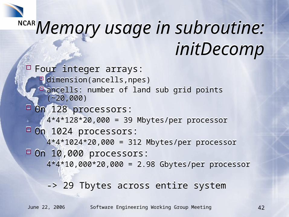
Memory usage in subroutine:initDecomp Four integer arrays:
dimension(ancells,npes) ancells: number of land sub grid points (~20,000)
On 128 processors:4*4*128*20,000 = 39 Mbytes/per processor
On 1024 processors:4*4*1024*20,000 = 312 Mbytes/per processor
On 10,000 processors:4*4*10,000*20,000 = 2.98 Gbytes/per processor
-> 29 Tbytes across entire system
Four integer arrays: dimension(ancells,npes) ancells: number of land sub grid points (~20,000)
On 128 processors:4*4*128*20,000 = 39 Mbytes/per processor
On 1024 processors:4*4*1024*20,000 = 312 Mbytes/per processor
On 10,000 processors:4*4*10,000*20,000 = 2.98 Gbytes/per processor
-> 29 Tbytes across entire system

June 22, 2006 Software Engineering Working Group Meeting 43
Memory use in CLMMemory use in CLM
Subroutine initDecomp deallocates large arrays
CLM Configuration:1x1.25 gridNo RTMMAXPATCH_PFT = 4No CN, DGVM
Measure stack and heap on 32-512 BG/L processors
Subroutine initDecomp deallocates large arrays
CLM Configuration:1x1.25 gridNo RTMMAXPATCH_PFT = 4No CN, DGVM
Measure stack and heap on 32-512 BG/L processors

June 22, 2006 Software Engineering Working Group Meeting 44
Memory use for CLM on BG/L
Memory use for CLM on BG/L
June 22, 2006 Software Engineering Working Group Meeting 45
Non-scalable memory usage
Non-scalable memory usage
Common problemEasy to ignore on 128 processorsFatal on large processor counts
Avoid array dimension with npesFixed size
Eliminate serial code!!Re-evaluate initialization code (scalable?)Remember:
Innocent looking non-scalable code can kill!
Common problemEasy to ignore on 128 processorsFatal on large processor counts
Avoid array dimension with npesFixed size
Eliminate serial code!!Re-evaluate initialization code (scalable?)Remember:
Innocent looking non-scalable code can kill!

June 22, 2006 Software Engineering Working Group Meeting 46
Outline:Outline:
Motivation POP CICE CLM CAM + Coupler Conclusions
Motivation POP CICE CLM CAM + Coupler Conclusions

June 22, 2006 Software Engineering Working Group Meeting 47
CAM + CouplerCAM + Coupler
CAMExtensive benchmarking [P. Worley]Generalizing interface for modular dynamics
Non lat-lon grids [B. Eaton]Quasi uniform grids (cubed-sphere, icoshedral)
Ported to BGL [S. Ghosh]Required rewrite on I/OFV-core resolution limited due to memory
CouplerWill examine single executable concurrent
system (Summer 06)

June 22, 2006 Software Engineering Working Group Meeting 48
A Petascale coupled system
A Petascale coupled system
Design principles:Simple/elegant designAttention to implementation detailsSingle executable -> run on any thing
vendors provideminimizes communication hotspots
Concurrent execution creates hotspotsE.G. waste bisection bandwidth by passing
fluxes to coupler
Design principles:Simple/elegant designAttention to implementation detailsSingle executable -> run on any thing
vendors provideminimizes communication hotspots
Concurrent execution creates hotspotsE.G. waste bisection bandwidth by passing
fluxes to coupler

June 22, 2006 Software Engineering Working Group Meeting 49
A Petascale coupled system (con’t)
A Petascale coupled system (con’t)
Sequential executionFlux interpolation just a boundary exchangeSimplifies cost budgetAll components must be scalable
Quasi-uniform gridFlux interpolation should be communication
with small number of nearest neighborsMinimizes interpolation costs
Sequential executionFlux interpolation just a boundary exchangeSimplifies cost budgetAll components must be scalable
Quasi-uniform gridFlux interpolation should be communication
with small number of nearest neighborsMinimizes interpolation costs

June 22, 2006 Software Engineering Working Group Meeting 50
Possible ConfigurationPossible Configuration
CAM (100 km, L66)POP @ 0.1 degree
Demonstrated 30 seconds per day
Sea-Ice @ 0.1 degree Land model (50 km)Sequential Coupler
CAM (100 km, L66)POP @ 0.1 degree
Demonstrated 30 seconds per day
Sea-Ice @ 0.1 degree Land model (50 km)Sequential Coupler

June 22, 2006 Software Engineering Working Group Meeting 51
High-Resolution CCSM on ~30K BG/L processors
High-Resolution CCSM on ~30K BG/L processors
Time per day (secs)
demonstrated Budget Actual
[email protected] Yes [03/29/06] 30 30.1
[email protected] No [Summer 06] 8
Land (50 km)
No [Summer 06] 5
Atm + Chem(100 km)
No [Fall 06] 77
Coupler No [Fall 06] 10
Total No [Spring 07] 130
~1.8 years/wallclock day

June 22, 2006 Software Engineering Working Group Meeting 52
ConclusionsConclusions
Examine scalability of several components on BG/LStress limits of resolution and processor countUncover problems in code
Is possible to use large # proc POP @ 0.1Results obtain by modifying ~9 filesBGW 30K proc --> 7.9 years/wallclock day
33% of time in 3D-update -> CICE boundary exchange
RedStorm 8K proc--> 8.1 years/wallclock day50% of time in solver -> use preconditioner

June 22, 2006 Software Engineering Working Group Meeting 53
Conclusions (con’t)Conclusions (con’t)
CICE needs Improved load-balancing (w-SFC)
CLM needs Parallelize RTM, I/O Cleanup non-scalable data structures
Common Issues: Focus on returning advances into models
Vector mods in POP? Parallel I/O in CAM? High-resolution CRIEPI work?
Parallel I/O Eliminate all serial code! Watch the memory usage
CICE needs Improved load-balancing (w-SFC)
CLM needs Parallelize RTM, I/O Cleanup non-scalable data structures
Common Issues: Focus on returning advances into models
Vector mods in POP? Parallel I/O in CAM? High-resolution CRIEPI work?
Parallel I/O Eliminate all serial code! Watch the memory usage

June 22, 2006 Software Engineering Working Group Meeting 54
Conclusions (con’t)Conclusions (con’t)
Efficient use of Petascale system is possible!
Path to Petascale computing:1. Test the limits of our codes2. Fix resulting problems3. Goto 1.
Efficient use of Petascale system is possible!
Path to Petascale computing:1. Test the limits of our codes2. Fix resulting problems3. Goto 1.

June 22, 2006 Software Engineering Working Group Meeting 55
Acknowledgements/Questions?
Acknowledgements/Questions?
Thanks to: D. Bailey (NCAR)F. Bryan (NCAR)T. Craig (NCAR)J. Edwards (IBM)E. Hunke (LANL)B. Kadlec (CU)E. Jessup (CU)P. Jones (LANL)K. Lindsay (NCAR)W. Lipscomb (LANL)M. Taylor (SNL)H. Tufo (NCAR)M. Vertenstein (NCAR)S. Weese (NCAR)P. Worley (ORNL)
Thanks to: D. Bailey (NCAR)F. Bryan (NCAR)T. Craig (NCAR)J. Edwards (IBM)E. Hunke (LANL)B. Kadlec (CU)E. Jessup (CU)P. Jones (LANL)K. Lindsay (NCAR)W. Lipscomb (LANL)M. Taylor (SNL)H. Tufo (NCAR)M. Vertenstein (NCAR)S. Weese (NCAR)P. Worley (ORNL)
Computer Time: Blue Gene/L time:
NSF MRI GrantNCARUniversity of ColoradoIBM (SUR) program
BGW Consortium DaysIBM research (Watson)
LLNL RedStorm time:
Sandia
Computer Time: Blue Gene/L time:
NSF MRI GrantNCARUniversity of ColoradoIBM (SUR) program
BGW Consortium DaysIBM research (Watson)
LLNL RedStorm time:
Sandia
et

June 22, 2006 Software Engineering Working Group Meeting 56
eta1_local=0.0D0
do i=1,nActive
Z(i) = Minv2(i)*R(i) ! Apply the diagonal preconditioner
eta1_local = eta1_local + R(i)*Z(i) !*** (r,(PC)r)
enddo
Z(iptrHalo:n) = Minv2(iptrHalo:n)*R(iptrHalo:n)
!-----------------------------------------------------------------------
! update conjugate direction vector s
!-----------------------------------------------------------------------
if(lprecond) call update_halo(Z)
eta1 = global_sum(eta1_local,distrb_tropic)
cg_beta = eta1/eta0
do i=1,n
S(i) = Z(i) + S(i)*cg_beta
enddo
call matvec(n,A,Q,S)
!-----------------------------------------------------------------------
! compute next solution and residual
!-----------------------------------------------------------------------
call update_halo(Q)
eta0 = eta1
rtmp_local = 0.0D0
do i=1,nActive
rtmp_local = rtmp_local + Q(i)*S(i)
enddo
rtmp = global_sum(rtmp_local,distrb_tropic)
eta1 = eta0/rtmp
do i=1,n
X(i) = X(i) + eta1*S(i)
R(i) = R(i) - eta1*Q(i)
enddo

June 22, 2006 Software Engineering Working Group Meeting 57
do iblock=1,nblocks_tropic this_block = get_block(blocks_tropic(iblock),iblock) if (lprecond) then call preconditioner(WORK1,R,this_block,iblock) else
where(A0(:,:,iblock /= c0) then WORK1(:,:,iblock) = R(:,:,iblock)/A0(:,:,iblock)
elsewhereWORK1(:,:,iblock) = c0
endwhere endif WORK0(:,:,iblock) = R(:,:,iblock)*WORK1(:,:,iblock) end do ! block loop!----------------------------------------------------------------------! update conjugate direction vector s!-----------------------------------------------------------------------if (lprecond) & call update_ghost_cells(WORK1,bndy_tropic, field_loc_center,& field_type_scalar) !*** (r,(PC)r) eta1 = global_sum(WORK0, distrb_tropic, field_loc_center, RCALCT_B)
do iblock=1,nblocks_tropic this_block = get_block(blocks_tropic(iblock),iblock) S(:,:,iblock) = WORK1(:,:,iblock) + S(:,:,iblock)*(eta1/eta0)!----------------------------------------------------------------------! compute As!----------------------------------------------------------------------- call btrop_operator(Q,S,this_block,iblock) WORK0(:,:,iblock) = Q(:,:,iblock)*S(:,:,iblock) end do ! block loop!-----------------------------------------------------------------------! compute next solution and residual!----------------------------------------------------------------------- call update_ghost_cells(Q, bndy_tropic, field_loc_center, & field_type_scalar eta0 = eta1 eta1 = eta0/global_sum(WORK0, distrb_tropic, & field_loc_center, RCALCT_B) do iblock=1,nblocks_tropic this_block = get_block(blocks_tropic(iblock),iblock) X(:,:,iblock) = X(:,:,iblock) + eta1*S(:,:,iblock) R(:,:,iblock) = R(:,:,iblock) - eta1*Q(:,:,iblock) if (mod(m,solv_ncheck) == 0) then call btrop_operator(R,X,this_block,iblock) R(:,:,iblock) = B(:,:,iblock) - R(:,:,iblock) WORK0(:,:,iblock) = R(:,:,iblock)*R(:,:,iblock) endif end do ! block loop

June 22, 2006 Software Engineering Working Group Meeting 58
Piece 1D data structure solver
Piece 1D data structure solver
!-----------------------------------------------------! compute next solution and residual!----------------------------------------------------- call update_halo(Q) eta0 = eta1 rtmp_local = 0.0D0 do i=1,nActive rtmp_local = rtmp_local + Q(i)*S(i) enddo rtmp =
global_sum(rtmp_local,distrb_tropic) eta1 = eta0/rtmp do i=1,n X(i) = X(i) + eta1*S(i) R(i) = R(i) - eta1*Q(i) enddo
Update Halo
Dot product
Update vectors
ret

June 22, 2006 Software Engineering Working Group Meeting 59
POP 0.1 degreePOP 0.1 degreeblocksize
Nb Nb2 Max ||
36x24 100 10000 7545
30x20 120 14400 10705
24x16 150 22500 16528
18x12 200 40000 28972
15x10 240 57600 41352
12x8 300 90000 64074
Increasing || -->D
ecre
asin
g ov
erhe
ad -
->

June 22, 2006 Software Engineering Working Group Meeting 60
Serial Execution time on Multiple platforms (test)Serial Execution time on Multiple platforms (test)
0
1
2
3
4
5
6
7
8
9
10
IBM POWER4 IBM POWER5 IBM PPC 440 AMD Opteron Intel P4
(1.3 Ghz) (1.9 Ghz) (700 Mhz) (2.2 Ghz) (2.0 Ghz)
Compute Platform
seconds for 20 timesteps
PCG2+2D
PCG1+2D
PCG2+1D
PCG1+1D
0
1
2
3
4
5
6
7
8
9
10
IBM POWER4 IBM POWER5 IBM PPC 440 AMD Opteron Intel P4
(1.3 Ghz) (1.9 Ghz) (700 Mhz) (2.2 Ghz) (2.0 Ghz)
Compute Platform
seconds for 20 timesteps
PCG2+2D
PCG1+2D
PCG2+1D
PCG1+1D

June 22, 2006 Software Engineering Working Group Meeting 61
The Unexpected Problem:The Unexpected Problem:
Just because your code scales to N processors, does not mean it will scale to k*N, where k>=4.
Just because your code scales to N processors, does not mean it will scale to k*N, where k>=4.
Recommended