13
Basics of Genetic Algorithmsand some possibilities
Peter SpijkerTechnische Universiteit Eindhoven
Department of Biomedical EngineeringDivision of Biomedical Imaging and Modeling
California Institute of TechnologyMaterials Process and Simulation Center
Biochemistry & Molecular Biophysics
November 25, 2003
12

13Presentation Overview
• Purpose of presentation
• General introduction to Genetic Algorithms (GA’s)
• Biological background• Origin of species
• Natural selection
• Genetic Algorithm• Search space
• Basic algorithm
• Coding
• Methods
• Examples
• Possibilities

13Purpose of presentation
• Optimising parameters of force fields is a difficult and time consuming task
• Use of optimising methods might be of use
• Methods:- steepest descent
- simulated annealing (Monte Carlo)
- genetic algorithms
• Brief introduction to genetic algorithms in lecture style
13General Introduction to GA’s
• Genetic algorithms (GA’s) are a technique to solve problems which need optimization
• GA’s are a subclass of Evolutionary Computing
• GA’s are based on Darwin’s theory of evolution
• History of GA’s
• Evolutionary computing evolved in the 1960’s.
• GA’s were created by John Holland in the mid-70’s.

13Biological Background (1) – The cell
• Every animal cell is a complex of many small “factories” working together
• The center of this all is the cell nucleus
• The nucleus contains the genetic information

13Biological Background (2) – Chromosomes
• Genetic information is stored in the chromosomes
• Each chromosome is build of DNA
• Chromosomes in humans form pairs
• There are 23 pairs
• The chromosome is divided in parts: genes
• Genes code for properties
• The posibilities of the genesforone property is called: allele
• Every gene has an unique positionon the chromosome: locus

13Biological Background (3) – Genetics
• The entire combination of genes is called genotype
• A genotype develops to a phenotype
• Alleles can be either dominant or recessive
• Dominant alleles will always express from the genotype to the fenotype
• Recessive alleles can survive in the population for many generations, without being expressed.

13Biological Background (4) – Reproduction
• Reproduction of genetical information• Mitosis
• Meiosis
• Mitosis is copying the same genetic information to new
offspring: there is no exchange of
information
• Mitosis is the normal way ofgrowing of multicell structures,
like organs.

13Biological Background (5) – Reproduction
• Meiosis is the basis of sexual reproduction
• After meiotic division 2 gametesappear in the process
• In reproduction two gametesconjugate to a zygote wich
will become the new individual
• Hence genetic information is sharedbetween the parents in order to
create new offspring

13Biological Background (6) – Reproduction
• During reproduction “errors” occur
• Due to these “errors” genetic variation exists
• Most important “errors” are:
• Recombination (cross-over)
• Mutation

13Biological Background (7) – Natural selection
• The origin of species: “Preservation of favourablevariations and rejection of unfavourable
variations.”
• There are more individuals born than can survive, so there is a continuous struggle for life.
• Individuals with an advantage have a greater chance for survive: survival of the fittest.

13Biological Background (8) – Natural selection
• Important aspects in natural selection are:
• adaptation to the environment
• isolation of populations in different groups which cannot mutually mate
• If small changes in the genotypes of individuals are expressed easily, especially in small populations, we speak of genetic drift
• Mathematical expresses as fitness: success in life

13Presentation Overview
• Purpose of presentation
• General introduction to Genetic Algorithms (GA’s)
• Biological background• Origin of species
• Natural selection
• Genetic Algorithm• Search space
• Basic algorithm
• Coding
• Methods
• Examples
• Possibilities
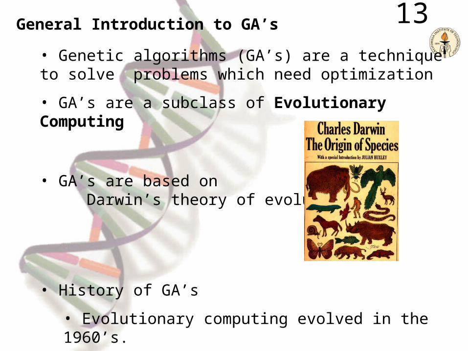
13Genetic Algorithm (1) – Search space
• Most often one is looking for the best solutionin a specific subset of solutions
• This subset is called the search space (or state space)
• Every point in the search space is a possible solution
• Therefore every point has a fitness value, depending on the problem definition
• GA’s are used to search thesearch space for the best
solution, e.g. a minimum
• Difficulties are the local minima and the starting
point of the search
0 100 200 300 400 500 600 700 800 900 10000
0.5
1
1.5
2
2.5

13Genetic Algorithm (2) – Basic algorithm
• Starting with a subset of n randomly chosen solutions from the search space (i.e. chromosomes). This is the population
• This population is used to produce a next generation of individuals by reproduction
• Individuals with a higher fitness have more chance to reproduce (i.e. natural selection)

13Genetic Algorithm (3) – Basic algorithm
• Outline of the basic algorithm
0 START : Create random population of n chromosomes
1 FITNESS : Evaluate fitness f(x) of each chromosome in the population
2 NEW POPULATION
0 SELECTION : Based on f(x)
1 RECOMBINATION : Cross-over chromosomes
2 MUTATION : Mutate chromosomes
3 ACCEPTATION : Reject or accept new one
3 REPLACE : Replace old with new population: the new
generation
4 TEST : Test problem criterium
5 LOOP : Continue step 1 – 4 until criterium is satisfied

13Genetic Algorithm (4) – Coding
• Normal cells are diploid (containing 2 complete sets of chromosomes)
• On the contrary gametes are haploid
• Formalizing diploid reproduction is much more difficult than haploid
• Diploid populations have an extra dimension compared to haploid populations
• For simplicity therefore only haploid genetic algorithms
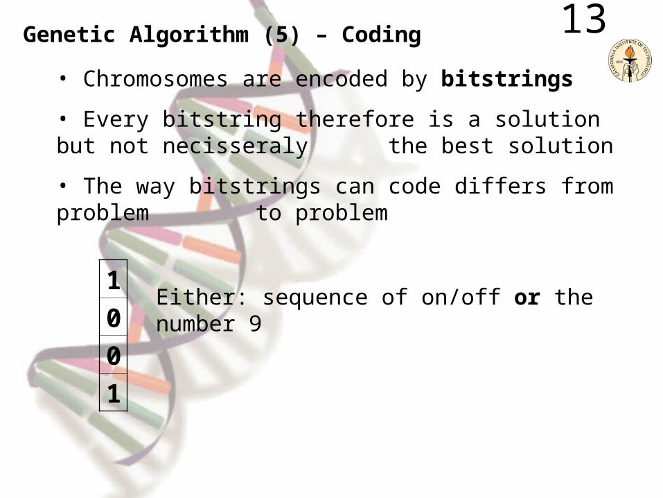
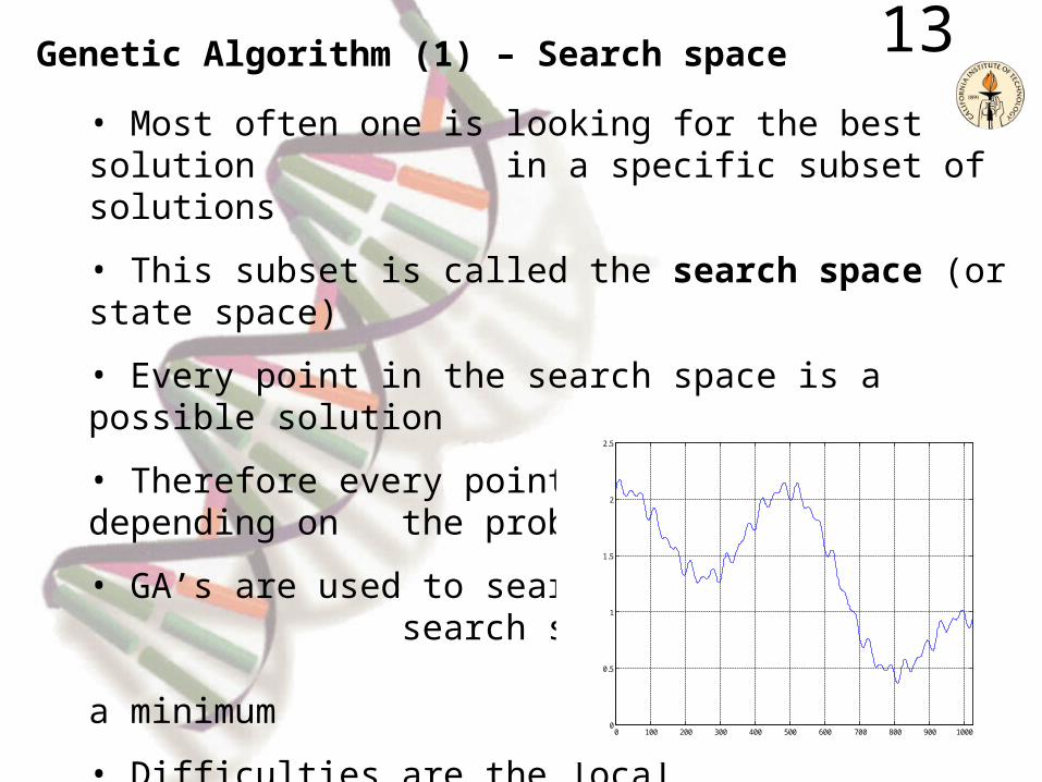
13Genetic Algorithm (5) – Coding
• Chromosomes are encoded by bitstrings
• Every bitstring therefore is a solution but not necisseraly the best solution
• The way bitstrings can code differs from problem to problem
Either: sequence of on/off or the number 91
0
0
1

13Genetic Algorithm (6) – Coding
• Recombination (cross-over) can when using bitstrings schematically be represented:
• Using a specific cross-over point
1
0
0
1
1
0
1
0
1
0
1
1
1
0
X
1
0
0
1
1
1
0
0
1
0
1
1
0
1

13Genetic Algorithm (7) – Coding
• Mutation prevents the algorithm to be trapped in a local minimum
• In the bitstring approach mutation is simpy the flipping of one of the bits
1
0
0
1
1
0
1
1
1
0
1
1
0
1

13Genetic Algorithm (8) – Coding
• Both recombination and mutation depend a loton the exact definition of the
problem and the choice of representing the chromosomes (e.g. no bitstrings)
• Different encodings can be used:• Binary encoding
• Permutation encoding
• Value encoding
• Tree encoding
• Focus in this presentation stays with binary encoding

13Example Minimum of Function (1)
• First example shows how to find the minimum of a function
0 100 200 300 400 500 600 700 800 900 10000
0.5
1
1.5
2
2.5
Minimum f(x) at x = 809
1100101001

13Example Minimum of Function (2)
0 200 400 600 800 1000 12000.2
0.4
0.6
0.8
1
1.2
1.4
1.6
1.8
2
2.2
Generation 1
0 10 20 30 40 50 60 70 800.3
0.4
0.5
0.6
0.7
0.8
0.9
1
1.1
1.2
1.3
Generations
Fitn
ess
Best FitnessMean Fitness
Individual Best individual
Mean fitness
Best fitness
Generations

13Example Minimum of Function (3)
• Interactive show of this algorithm with Matlab
• Using the function: genalg2()
• Variables:• Population size
• Bitstringlength
• Mutation chance
• Recombination chance
• Starting population adaption

13Genetic Algorithm (9) – Remarks
• It is clear from the example that the convergencespeed of the algorithm depends on
many factors:• Population size
• Mutation probability
• Recombination probability
• Elitism
• Selection methods• Random selection of parents
• Roulette wheel selection of parents
• Strong point GA’s: mutation prevents from falling in a local minimum, recombination initiates a fast first convergence

13Example Checkboard (1)
• We are given an n by n checkboard in which every field can have a different colour
from a set of four colours.
• Goal is to achieve a checkboard in a way that there are no neighbours with the same colour (not diagonal)
1 2 3 4 5 6 7 8 9 10
1
2
3
4
5
6
7
8
9
10
1 2 3 4 5 6 7 8 9 10
1
2
3
4
5
6
7
8
9
10

13Example Checkboard (2)
• Chromosomes represent the way the checkboardis coloured.
• Chromosomes are not represented by bitstrings but by bitmatrices
• The bits in the bitmatrix can have one of the four values 0, 1, 2 or 3, depending on the colour
• Crossing-over involves matrix manipulation instead of point wise operating. Crossing-over can be combining the parential matrices in a horizontal, vertical, triangular or square way
• Mutation remains bitwise changing bits in either one of the other numbers

13Example Checkboard (3)
• Fitnesscurve for the checkboard example
• This problem can be seen as a graph with n nodes and (n-1) edges, so the fitness f(x) is easily
defined as: f(x) = 2 · (n-1) ·n
0 100 200 300 400 500 600130
135
140
145
150
155
160
165
170
175
180
Generations
Fitn
ess
Best FitnessMean Fitness

13Example Checkboard (4)
• Fitnesscurves for different cross-over rules
0 100 200 300 400 500130
140
150
160
170
180
Fit
ne
ss
Lower-Triangular Crossing Over
0 200 400 600 800130
140
150
160
170
180Square Crossing Over
0 200 400 600 800130
140
150
160
170
180
Generations
Fit
ne
ss
Horizontal Cutting Crossing Over
0 500 1000 1500130
140
150
160
170
180
Generations
Verical Cutting Crossing Over

13Example Checkboard (5)
• Interactive show of this algorithm with Matlab
• Using the functions: • main()
• checkers()
• bestindividual()
• mutate()
• recombine()
• select()
• showbestindividual()
13Possibilities
• Using the genetic algorithm to optimise parameters for a force field
• Parameters are real numbers, so adaptations of these algorithms is required
• Value incoding vs. bitstring encoding
• Difficulties:• Definition fitness function
• Integration algorithm with software

13Further Questions
?
Recommended