7. Brownian Motion & Diffusion Processes
• A continuous time stochastic process with
(almost surely) continuous sample paths which
has the Markov property is called a diffusion.
• “almost surely” means “with probability 1”,
and we usually assume all sample paths are
continuous.
• The simplest and most fundamental diffusion
process is Brownian motion {B(t)}, which is
sometimes called the Wiener process {W (t)}.
Definition 1. {B(t)} is Brownian motion if it is
a diffusion process satisfying
(i) B(0) = 0,
(ii) E[
B(t)]
= 0 and Var[
B(t)]
= σ2t,
(iii) {B(t)} has stationary, independent
increments.
1
Applications of Diffusion Processes
• Many physical processes are continuous in space
and time. If all important variables are included
in the state of the system, then the future
evolution of the system should depend on the
current state, i.e., the system is Markovian.
• Any system with these properties is a diffusion,
by definition!
Examples: Molecular motion, stock market
fluctuations, communications systems,
neurophysiological processes.
• Discrete processes may be well approximated by
diffusions, in a limit as the discretization
becomes fine.
Examples: population growth models, disease
models, queuing models for large systems.
2
Brownian Motion as a limit of random walks
• Einstein (1905) showed how the motion of
pollen particles in water (Brown, 1827) could be
explained by a random walk due to random
bombardment of the pollen by water molecules.
• Set X1, X2, ... iid with E[X1] = 0, Var(X1) = σ2.
Define B(n)(t) when t a multiple of 1/n by
B(n)(t) =1√n
nt∑
i=1
Xi,
using linear interpolation to define B(n)(t)
between these times. Then,
• B(n)(0) = 0.
• E[B(n)(t)] = 0 and limn→∞ Var[B(n)(t)] = σ2t.
• {B(n)(t)} has stationary, independent
increments at the discrete times, t = k/n (and
hence, also, a discrete-time Markov property).
• {B(n)(t)} has continuous sample paths.
• One might expect Brownian motion in the limit
n → ∞. This was proved by Wiener (≈ 1915).
3

• Now apply the central limit theorem to
B(n)(t)−B(n)(s):
Definition 2. {B(t)} is Brownian motion if
(i) B(0) = 0,
(ii) {B(t)} has stationary, independent
increments,
(iii) B(t) ∼ N[
0, σ2t]
.
• Note: independent increments imply the
Markov property.
• Note: it can be shown that Definition 2 implies
almost surely continuous sample paths.
• Note: continuous sample paths lead to Gaussian
increments much as counting processes lead to
Poisson increments.
4

Hitting times and maximum of {B(t)}• {B(t)} is symmetric, i.e., {−B(t)} is also
Brownian motion and P[B(t) > 0] = 1/2. This
has useful consequences, for example:
Proposition. P[
max0≤s≤t
B(s) ≥ a]
= 2P[
B(t) ≥ a]
Proof
5
• Symmetry is also useful to study Z(t) = |B(t)|.{Z(t)} is called reflected Brownian motion.
Why?
• Find P[
Z(t) ≤ y]
and hence E[Z(t)], Var[Z(t)].
6
The joint distribution of Brownian motion
and its maximum
• Let M(t) = sup0≤s≤t
B(s). Show that, for y ≥ x,
P[
M(t)>y,B(t)<x]
=
∫ ∞
2y−x
1√2πt
exp{
−u2
2t
}
du.
7

Gaussian Processes and Gaussian Diffusions
• Y = (Y1, . . . , Yn) is multivariate normal if
Y = µ+AZ where µ is a vector in Rn, A is an
n×m matrix and Z = (Z1, . . . , Zm) is a random
vector of iid standard normal variables. We write
Y ∼ N[
µ,AAT]
where µ = E[Y ] and
AAT = Var(Y ) = E[(
Y − E[Y ])(
Y − E[Y ])T ]
.
• {X(t), t ≥ 0} is a Gaussian process if
(X(t1), X(t2), . . . , X(tn)) is multivariate Normal
for all t1, . . . , tn.
• Since the multivariate normal distribution is
specified by its mean and covariance matrix, a
Gaussian process is specified by its mean
function µ(t) = E[X(t)] and covariance
function γ(s, t) = Cov(X(s), X(t))
• Gaussian processes are not usually diffusions.
Why?
8

Brownian motion as a Gaussian process:{B(t)} is a Gaussian process, from Definition 2.
Clearly, µ(t) = 0. Find γ(s, t).
9

Conditioning a diffusion on its future value
• Let {X(t)} be a diffusion. Let {Z(t), 0 ≤ t ≤ 1}correspond to X(t) conditioned on X(1) = α.
Show that {Z(t)} is a diffusion.
• Note that a homogeneous diffusion, where
the transition probabilities do not depend on
time, becomes inhomogeneous once
conditioned on a future value.
10

Conditioning a Gaussian process on
its future value
• Let {X(t)} be a Gaussian process. Let
{Z(t), 0 ≤ t ≤ 1} correspond to {X(t)}conditioned on X(1)=α. Show that {Z(t)} is a
Gaussian process.
11

The Brownian bridge
Let {Z(t), 0 ≤ t ≤ 1}have the distribution
of {B(t)} conditioned
on B(1)= 0, where
{B(t)} is standard
Brownian motion.
Then {Z(t)} is a
Brownian bridge.
• {Z(t)} is a Gaussian diffusion process. Find its
mean and covariance functions.
Solution
12

Solution continued
13

Another construction of the Brownian bridge
For {B(t)} standard Brownian motion, set
Z(t) = B(t)− tB(1). Show that {Z(t)} is a
Brownian bridge.
Solution
14
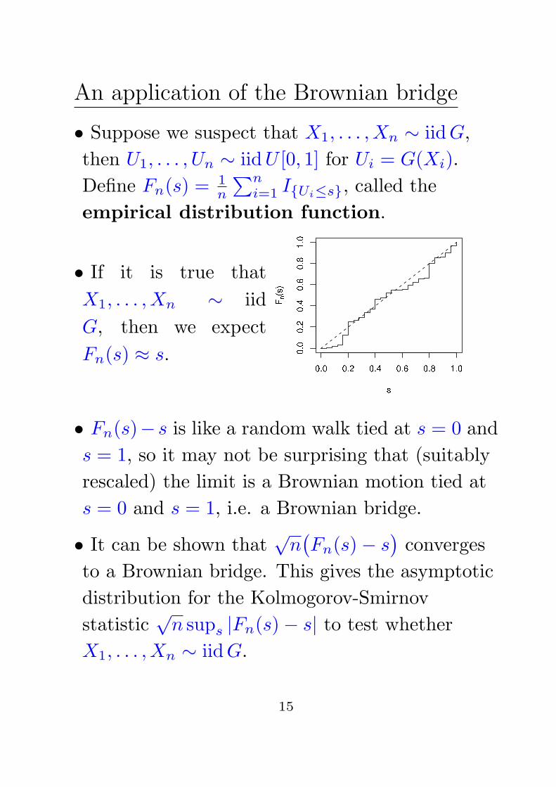
An application of the Brownian bridge
• Suppose we suspect that X1, . . . , Xn ∼ iidG,
then U1, . . . , Un ∼ iidU [0, 1] for Ui = G(Xi).
Define Fn(s) =1n
∑ni=1 I{Ui≤s}, called the
empirical distribution function.
• If it is true that
X1, . . . , Xn ∼ iid
G, then we expect
Fn(s) ≈ s.
• Fn(s)− s is like a random walk tied at s = 0 and
s = 1, so it may not be surprising that (suitably
rescaled) the limit is a Brownian motion tied at
s = 0 and s = 1, i.e. a Brownian bridge.
• It can be shown that√n(
Fn(s)− s)
converges
to a Brownian bridge. This gives the asymptotic
distribution for the Kolmogorov-Smirnov
statistic√n sups |Fn(s)− s| to test whether
X1, . . . , Xn ∼ iidG.
15
R code for a Brownian bridge
np=1000
t=seq(from=0,to=1,length=np)
X=cumsum(rnorm(np,mean=0,sd=sqrt(1/np)))
Z=X-t*X[np]
plot(t,Z,type="l")
abline(h=0,lty="dashed")
R code for the empirical cdf
np=25
t=seq(np)/np
U=runif(np)
F=sort(U)
plot(x=c(0,rep(t,each=2),1,1),
y=c(0,0,rep(F,each=2),1),
xlab=’s’,
ylab=expression(paste(F[n],"(s)")),
ty="l")
lines(c(0,1),c(0,1),lty="dashed")
16
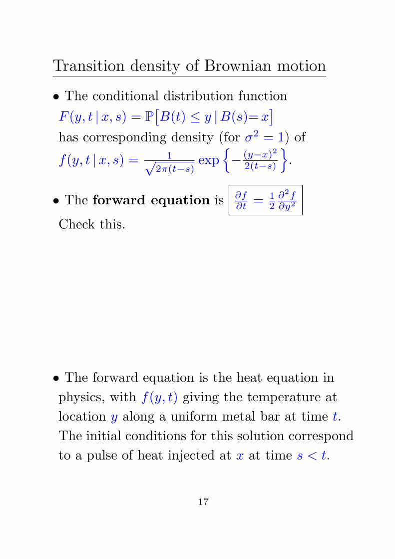
Transition density of Brownian motion
• The conditional distribution function
F (y, t |x, s) = P[
B(t) ≤ y |B(s)=x]
has corresponding density (for σ2 = 1) of
f(y, t |x, s) = 1√2π(t−s)
exp{
− (y−x)2
2(t−s)
}
.
• The forward equation is ∂f∂t = 1
2∂2f∂y2
Check this.
• The forward equation is the heat equation in
physics, with f(y, t) giving the temperature at
location y along a uniform metal bar at time t.
The initial conditions for this solution correspond
to a pulse of heat injected at x at time s < t.
17

• The backward equation for standard
Brownian motion is ∂f∂s = − 1
2∂2f∂x2
• We can derive similar equations for general
diffusion {X(t)}. It turns out that the forward
and backward equations only depend on the
infinitesimal mean or drift
µ(x, t) = limδt→0
E[
X(t+ δt)−X(t) |X(t)=x]
δt
and the infinitesimal variance
σ2(x, t) = limδt→0
E[(
X(t+ δt)−X(t))2 |X(t)=x
]
δt.
• Assuming sufficient regularity for the above
limits to exist and for the forward and backward
equations to have a unique solution (subject to
appropriate boundary conditions), a diffusion
is fully specified by its infinitesimal mean
and variance
18
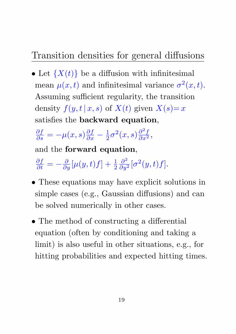
Transition densities for general diffusions
• Let {X(t)} be a diffusion with infinitesimal
mean µ(x, t) and infinitesimal variance σ2(x, t).
Assuming sufficient regularity, the transition
density f(y, t |x, s) of X(t) given X(s)=x
satisfies the backward equation,
∂f∂s = −µ(x, s)∂f∂x − 1
2σ2(x, s)∂
2f∂x2 ,
and the forward equation,
∂f∂t = − ∂
∂y [µ(y, t)f ] +12
∂2
∂y2 [σ2(y, t)f ].
• These equations may have explicit solutions in
simple cases (e.g., Gaussian diffusions) and can
be solved numerically in other cases.
• The method of constructing a differential
equation (often by conditioning and taking a
limit) is also useful in other situations, e.g., for
hitting probabilities and expected hitting times.
19

The backward equation can be derived based on
the identity
f(y, t |x, s) = E[
f(
y, t |X(s+ h), s+ h)
|X(s)=x]
followed by a Taylor series expansion about h = 0.
Solution
20

Example. Calculate the infinitesimal mean and
variance for a Brownian bridge, i.e., a Gaussian
diffusion {Z(t), 0 ≤ t ≤ 1} with E[Z(t)] = 0 and
Cov(Z(s), Z(t)) = s ∧ t− st.
21
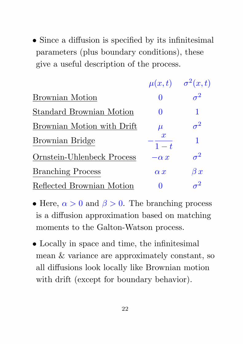
• Since a diffusion is specified by its infinitesimal
parameters (plus boundary conditions), these
give a useful description of the process.
µ(x, t) σ2(x, t)
Brownian Motion 0 σ2
Standard Brownian Motion 0 1
Brownian Motion with Drift µ σ2
Brownian Bridge − x
1− t1
Ornstein-Uhlenbeck Process −αx σ2
Branching Process αx β x
Reflected Brownian Motion 0 σ2
• Here, α > 0 and β > 0. The branching process
is a diffusion approximation based on matching
moments to the Galton-Watson process.
• Locally in space and time, the infinitesimal
mean & variance are approximately constant, so
all diffusions look locally like Brownian motion
with drift (except for boundary behavior).
22
Martingales to Study Brownian Motion
• Since martingale arguments are useful for
random walks, we expect them to help for the
continuous time analog, i.e., Brownian motion.
• We assume that the stopping theorem also
applies in continuous time.
(a) Note that B(t) is itself a martingale.
(b) [B(t)]2 − t is a martingale. Why?
23

(c) exp{cB(t)− c2t/2} is a martingale for any c.
Why?
24
Hitting Times for Brownian Motion
with Drift
• X(t) = B(t) + µt is called Brownian motion
with drift. Here, we take {B(t)} to be standard
Brownian motion, σ2 = 1.
• Let T = min {t : X(t) = A or X(t) = −B}. Therandom walk analog of T was important for
queuing and insurance ruin problems, so T is
important if such processes are modeled as
diffusions.
• (i) X(t)− µt is a martingale.
Also, exp{
c(X(t)− µt)− c2t/2}
is a martingale.
Taking c = −2µ gives
(ii) exp{−2µX(t)} is a martingale.
• We can use (i) and (ii) to find E[
T]
and
P[
X(T )=A]
via the martingale stopping
theorem.
25
• Because of continuous sample paths, there is no
issue of overshoot or undershoot. Unlike the
random walk case, the Martingale solution is
exact.
26

• E(T ) and P[X(T )=A] can also be calculated by
setting up & solving appropriate differential
equations (see Ross, Section 8.4).
• Also, these quantities can be found by taking a
limit of random walks. Let Y1, Y2, . . . be iid with
E[Yi] = 0, Var(Yi) = 1 and let
X [n](t) = 1√n
∑nti=1(Yi +
µ√n) for t = k/n, using
linear interpolation for t 6= k/n.
• The random walk converges to a diffusion
process, and we can check the infinitesimal mean
and variance of the limit to show that X [n](t)
converges in distribution to Brownian motion
with drift, X(t).
• Let X[n]k = 1√
n
∑ki=1
(
Yi +µ√n
)
and let
T [n] = min{
k : X[n]k ≥ A or X
[n]k ≤ −B
}
.
Then,
E[
T]
= limn→∞ E[
T [n]]/
n
and
P[
X(T )=A]
= limn→∞ P[X[n])
T [n] ≥ A],
assuming the excess is neglibible in the limit.
27
• Our previous results for the random walk are
P[
X[n]
T [n] ≥ A]
= PA ≈ 1− e−θnB
eθnA − e−θnB
E[
T [n]]
≈ APA −B(1− PA)
E[
1√n(Y1 +
µ√n)]
• Show that θn = −2µ+ o(1), i.e., limn θn = −2µ
• Completing this calculation is one way to do
Problem 8.15(c) in Ross.
28

Diffusions as solutions to
Stochastic Differential Equations
• The local properties of {X(t)} suggest that we
can write
X(t+h) = X(t) + µ(
X(t), t)
h +
σ(
X(t), t)[
B(t+h)−B(t)]
+ o(h).
• Dividing by h and taking a limit suggests
ddtX(t) = µ
(
X(t), t)
+ σ(
X(t), t)
ddtB(t).
• But this derivative is not defined, in the usual
sense, since sample paths of B(t) are not
differentiable. Why?
29

• To recognize the lack of differentiability, we
write dX(t) = µ(X(t), t) dt+ σ(X(t), t) dB(t).
The solution to this stochastic differential
equation (SDE) corresponds to a stochastic
integral equation,
X(t) = X(0)+
∫ t
0
{
µ(X(s), s)ds+σ(X(s), s)dB(s)}
.
• A stochastic integral can be defined analogously
to the Riemannn integral:∫ t
0
f(s) dB(s) = limN→∞
N−1∑
n=0
f(
tnN
)
[
B( t(n+1)
N
)
−B(
tnN
)
]
.
• We note some stochastic calculus results:
Supposing f(s) is sufficiently regular and f(s) is
independent of {B(t), t ≥ s},
(i)∫ t
0f(s) dB(s) has continuous sample paths.
(ii) E[ ∫ t
0f(s) dB(s)
]
= 0. .
(iii) Var[ ∫ t
0f(s) dB(s)
]
= E[ ∫ t
0[f(s)]2 ds
]
.
(iv) Cov[ ∫ t
0f(s) dB(s),
∫ t
0g(s) dB(s)
]
= E[ ∫ t
0f(s) g(s) ds
]
.
30
• We can use these properties to check that the
solution to
dX(t) = µ(
X(t), t)
dt+ σ(
X(t), t)
dB(t)
is a diffusion with infinitesimal parameters
µ(x, t) and σ2(x, t).
Solution
31

Transformations of Diffusions
• If {X(t)} is a time-homogeneous diffusion with
infinitesimal parameters µX(x) and σ2X(x), then
Y (t) = f(X(t)) is also a time-homogeneous
diffusion if f is invertible and continous. Why?
• Supposing f(x) is twice differentiable, the
infinitesimal parameters of Y (t) are
µY (y) = µX(x)f ′(x) + 12σ
2X(x)f ′′(x)
σ2Y (y) = σ2
X(x)[f ′(x)]2
where x = f−1(y), f ′ = dfdx , f
′′ = d2fdx2 .
• This transformation formula is different from
the non-stochastic “chain rule” for y = f(x),
namely dydt = df
dxdxdt . In SDE notation,
dY (t) = dfdx dX(t) + 1
2σ2X
d2fdx2 dt.
32

Derivation of the transformation formula.
33
Ornstein-Uhlenbeck process (O-U process)
• If a small particle is suspended in a liquid or
gas, then bombardment by molecules of the
medium should (by Newton’s laws) make the
velocity follow a random walk. However, the
particule also suffers friction (viscous drag)
which is approximately proportional to velocity.
This suggests an equation
dv(t) = −αv(t) dt+ σ dB(t)
with location then given by
x(t) = x(0) +∫ t
0v(s) ds,
which is equivalent to
dx(t) = v(t) dt.
• The Ornstein-Uhlenbeck process is a
diffusion on [−∞,∞] with infinitesimal
parameters µ(x, t) = −αx and σ2(x, t) = σ2.
34

• Let X(t) = e−αtX(0) +∫ t
0σe−α(t−s) dB(s).
Assuming that differentiation of stochastic
integrals follows the same rules as standard
deterministic integrals, show that X(t) is an O-U
process.
• This integral shows that the O-U process is a
linear function of Brownian motion, and so the
O-U process is a Gaussian process. (as long as
X(0) has a normal distribution).
35
• Find the mean and covariance functions for the
O-U process using the integral representation
and the properties (ii) and (iv) of stochastic
integrals. Suppose X(t) is stationary, so that
X(t) =∫ t
−∞ σe−α(t−s) dB(s).
• Note: Another way to do this is to use the
representation X(t) = σ e−αt/2 B(αeαt) where
{B(t)} is standard Brownian motion (see
homework).
36
Exponential Brownian Motion
• Let Y (t) = exp {σB(t) + µt}. This diffusionmodel is widely used in modeling the financial
markets and population growth.
• Find the infitiesimal parameters for {Y (t)} and
write down the SDE that it solves.
37

Diffusion approximation to a branching process
• Let X(t) be a branching process where each
individual reproduces at rate λ. Find a diffusion
approximation for large values of X(t).
38
Recommended