Previous Section Next Section
This is “Large Sample Tests for a Population Proportion”, section 8.5 from thebook Beginning Statistics (v. 1.0). For details on it (including licensing), clickhere.
For more information on the source of this book, or why it is available for free,please see the project's home page. You can browse or download additionalbooks there.
Has this book helped you? Consider passing it on:
Help Creative CommonsCreative Commons supports free culturefrom music to education. Their licenseshelped make this book available to you.
Help a Public SchoolDonorsChoose.org helps people like you
help teachers fund their classroomprojects, from art supplies to books to
calculators.
Table of Contents
8.5 Large Sample Tests for a Population Proportion
LEARNING OBJECTIVES
1. To learn how to apply the five-step critical value test procedure for test of
hypotheses concerning a population proportion.
2. To learn how to apply the five-step p-value test procedure for test of hypotheses
concerning a population proportion.
Both the critical value approach and the p-value approach can be applied to test
hypotheses about a population proportion p. The null hypothesis will have the
form 𝐻� : 𝑝 = 𝑝� for some specific number p0 between 0 and 1. The alternative
hypothesis will be one of the three inequalities 𝑝 < 𝑝�, 𝑝 > 𝑝
�, or 𝑝 ≠ 𝑝
� for the

same number p0 that appears in the null hypothesis.
The information in Section 6.3 "The Sample Proportion" in Chapter 6 "Sampling
Distributions" gives the following formula for the test statistic and its
distribution. In the formula p0 is the numerical value of p that appears in the
two hypotheses, 𝑞�= 1 − 𝑝
�, �̂� is the sample proportion, and n is the sample size.
Remember that the condition that the sample be large is not that n be at least
30 but that the interval
�̂�−3�̂�(1 − �̂�)
𝑛� , �̂� + 3
�̂�(1 − �̂�)
𝑛�
lie wholly within the interval [0,1] .
Standardized Test Statistic for Large Sample HypothesisTests Concerning a Single Population Proportion
The test statistic has the standard normal distribution.
The distribution of the standardized test statistic and the corresponding
rejection region for each form of the alternative hypothesis (left-tailed, right-
tailed, or two-tailed), is shown in Figure 8.14 "Distribution of the Standardized
Test Statistic and the Rejection Region".
Figure 8.14 Distribution of the Standardized Test Statistic and the Rejection Region
EXAMPLE 12
A soft drink maker claims that a majority of adults prefer its leading beverage over
that of its main competitor’s. To test this claim 500 randomly selected people were
given the two beverages in random order to taste. Among them, 270 preferred the
soft drink maker’s brand, 211 preferred the competitor’s brand, and 19 could not
make up their minds. Determine whether there is sufficient evidence, at the 5% level
of significance, to support the soft drink maker’s claim against the default that the
population is evenly split in its preference.
Solution:
We will use the critical value approach to perform the test. The same test will be
performed using the p-value approach in Note 8.49 "Example 14".
We must check that the sample is sufficiently large to validly perform the test. Since �̂�
= 270 ∕ 500 = 0.54,
�̂�(1 − �̂�)
𝑛� =
(0.54)(0.46)
500� ≈ 0.02
hence

��̂�−3 �̂(�−�̂)�� , �̂� + 3 �̂(�−�̂)
�� �
= [0.54 − (3)(0.02), 0.54 + (3)(0.02)]
= [0 . 48,0 . 60] ⊂ [0,1]
so the sample is sufficiently large.
Step 1. The relevant test is
𝐻� : 𝑝 = 0.50
vs. 𝐻� : 𝑝 > 0.50 @ 𝛼 = 0.05
where p denotes the proportion of all adults who prefer the company’s
beverage over that of its competitor’s beverage.
Step 2. The test statistic is
𝑍 =�̂� − 𝑝
�
�� ����
and has the standard normal distribution.
Step 3. The value of the test statistic is
𝑍 =�̂� − 𝑝
�
�� ����
=0.54 − 0.50
(����)(����)���
�
= 1.789
Step 4. Since the symbol in Ha is “>” this is a right-tailed test, so there is a single
critical value, 𝑧� = 𝑧���� . Reading from the last line in Figure 12.3 "Critical Values
of " its value is 1.645. The rejection region is [1.645,∞) .
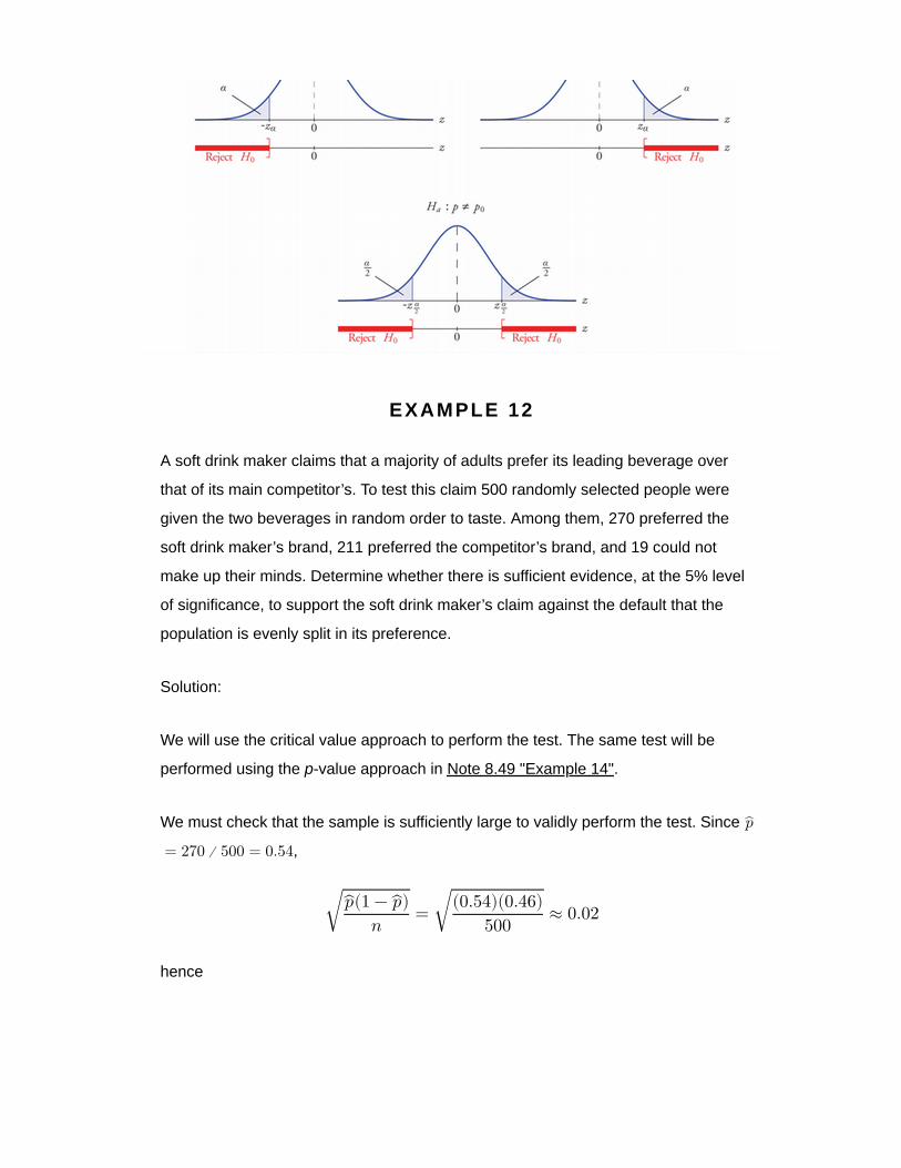
Step 5. As shown in Figure 8.15 "Rejection Region and Test Statistic for "
the test statistic falls in the rejection region. The decision is to reject H0. In
the context of the problem our conclusion is:
The data provide sufficient evidence, at the 5% level of significance, to
conclude that a majority of adults prefer the company’s beverage to that of
their competitor’s.
Figure 8.15
Rejection Region
and Test Statistic
for Note 8.47
"Example 12"
EXAMPLE 13
Globally the long-term proportion of newborns who are male is 51.46%. A researcher
believes that the proportion of boys at birth changes under severe economic
conditions. To test this belief randomly selected birth records of 5,000 babies born
during a period of economic recession were examined. It was found in the sample
that 52.55% of the newborns were boys. Determine whether there is sufficient
evidence, at the 10% level of significance, to support the researcher’s belief.
Solution:
We will use the critical value approach to perform the test. The same test will be
performed using the p-value approach in Note 8.50 "Example 15".
The sample is sufficiently large to validly perform the test since
�̂�(1 − �̂�)
𝑛� =
(0.5255)(0.4745)
5000� ≈ 0.01
hence
��̂�−3 �̂(�−�̂)�� , �̂� + 3 �̂(�−�̂)
�� �
= [0.5255 − 0 . 03,0 . 5255 + 0.03]
= [0 . 4955,0 . 5555] ⊂ [0,1]
Step 1. Let p be the true proportion of boys among all newborns during the
recession period. The burden of proof is to show that severe economic
conditions change it from the historic long-term value of 0.5146 rather than
to show that it stays the same, so the hypothesis test is
𝐻� : 𝑝 = 0.5146
vs. 𝐻� : 𝑝 ≠ 0.5146 @ 𝛼 = 0.10
Step 2. The test statistic is
𝑍 =�̂� − 𝑝
�
�� ����
and has the standard normal distribution.
Step 3. The value of the test statistic is
𝑍 =�̂� − 𝑝
�
�� ����
=0.5255 − 0.5146
(������)(������)����
�
= 1.542
Step 4. Since the symbol in Ha is “≠” this is a two-tailed test, so there are a pair of
critical values, ±𝑧�∕� = ± 𝑧���� = ± 1.645 . The rejection region is (−∞,−1.645]
∪ [1.645,∞) .
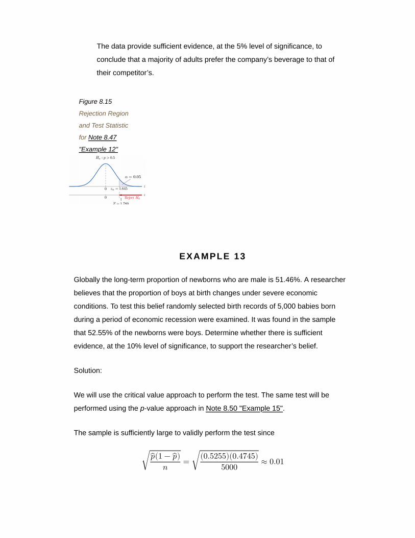
Step 5. As shown in Figure 8.16 "Rejection Region and Test Statistic for "
the test statistic does not fall in the rejection region. The decision is not to
reject H0. In the context of the problem our conclusion is:
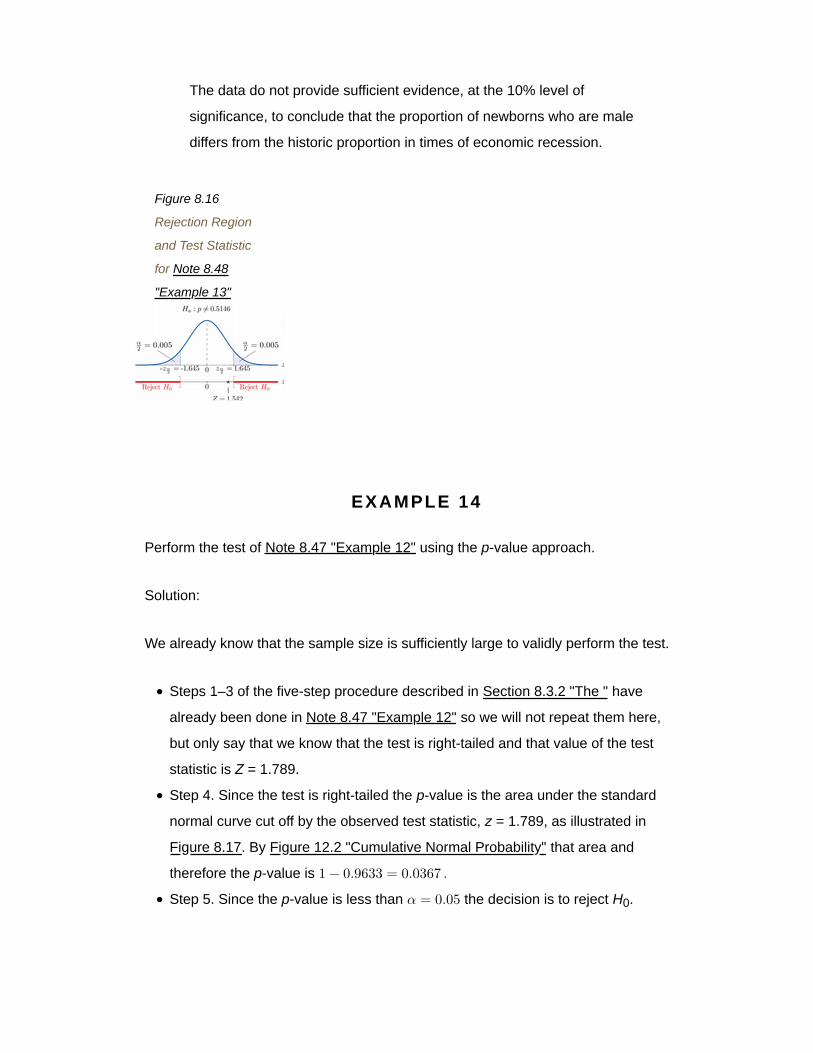
The data do not provide sufficient evidence, at the 10% level of
significance, to conclude that the proportion of newborns who are male
differs from the historic proportion in times of economic recession.
Figure 8.16
Rejection Region
and Test Statistic
for Note 8.48
"Example 13"
EXAMPLE 14
Perform the test of Note 8.47 "Example 12" using the p-value approach.
Solution:
We already know that the sample size is sufficiently large to validly perform the test.
Steps 1–3 of the five-step procedure described in Section 8.3.2 "The " have
already been done in Note 8.47 "Example 12" so we will not repeat them here,
but only say that we know that the test is right-tailed and that value of the test
statistic is Z = 1.789.
Step 4. Since the test is right-tailed the p-value is the area under the standard
normal curve cut off by the observed test statistic, z = 1.789, as illustrated in
Figure 8.17. By Figure 12.2 "Cumulative Normal Probability" that area and
therefore the p-value is 1 − 0.9633 = 0.0367 .
Step 5. Since the p-value is less than 𝛼 = 0.05 the decision is to reject H0.
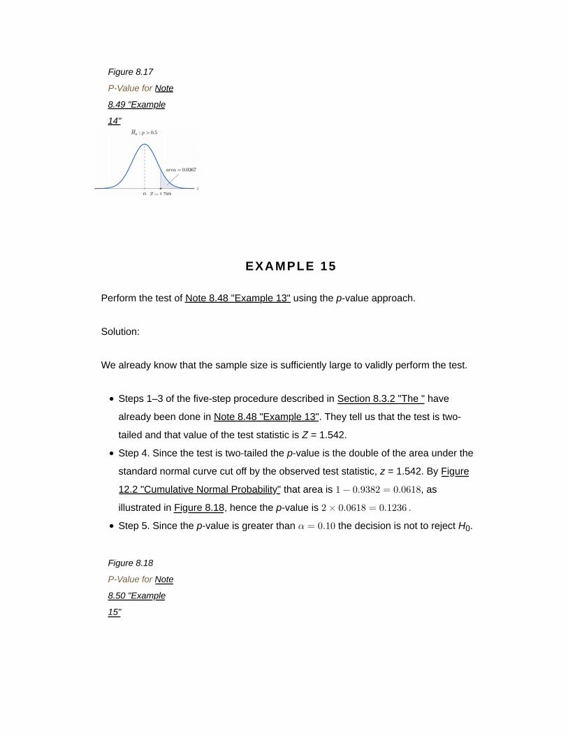
Figure 8.17
P-Value for Note
8.49 "Example
14"
EXAMPLE 15
Perform the test of Note 8.48 "Example 13" using the p-value approach.
Solution:
We already know that the sample size is sufficiently large to validly perform the test.
Steps 1–3 of the five-step procedure described in Section 8.3.2 "The " have
already been done in Note 8.48 "Example 13". They tell us that the test is two-
tailed and that value of the test statistic is Z = 1.542.
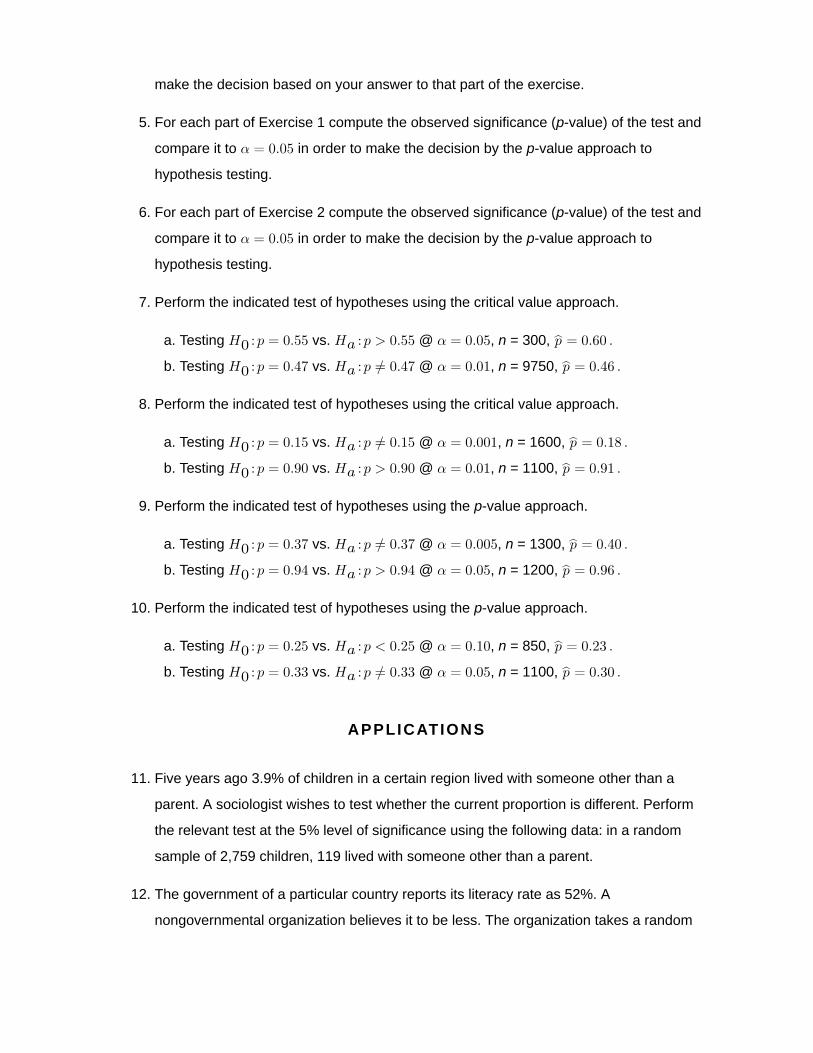
Step 4. Since the test is two-tailed the p-value is the double of the area under the
standard normal curve cut off by the observed test statistic, z = 1.542. By Figure
12.2 "Cumulative Normal Probability" that area is 1 − 0.9382 = 0.0618, as
illustrated in Figure 8.18, hence the p-value is 2 × 0.0618 = 0.1236 .
Step 5. Since the p-value is greater than 𝛼 = 0.10 the decision is not to reject H0.
Figure 8.18
P-Value for Note
8.50 "Example
15"

KEY TAKEAWAYS
There is one formula for the test statistic in testing hypotheses about a population
proportion. The test statistic follows the standard normal distribution.
Either five-step procedure, critical value or p-value approach, can be used.
EXERCISES
BASIC
On all exercises for this section you may assume that the sample is sufficiently large
for the relevant test to be validly performed.
1. Compute the value of the test statistic for each test using the information given.
a. Testing 𝐻�:𝑝 = 0.50 vs. 𝐻�:𝑝 > 0.50, n = 360, �̂� = 0.56 .
b. Testing 𝐻�:𝑝 = 0.50 vs. 𝐻�:𝑝 ≠ 0.50, n = 360, �̂� = 0.56 .
c. Testing 𝐻�:𝑝 = 0.37 vs. 𝐻�:𝑝 < 0.37, n = 1200, �̂� = 0.35 .
2. Compute the value of the test statistic for each test using the information given.
a. Testing 𝐻�:𝑝 = 0.72 vs. 𝐻�:𝑝 < 0.72, n = 2100, �̂� = 0.71 .
b. Testing 𝐻�:𝑝 = 0.83 vs. 𝐻�:𝑝 ≠ 0.83, n = 500, �̂� = 0.86 .
c. Testing 𝐻�:𝑝 = 0.22 vs. 𝐻�:𝑝 < 0.22, n = 750, �̂� = 0.18 .
3. For each part of Exercise 1 construct the rejection region for the test for 𝛼 = 0.05 and
make the decision based on your answer to that part of the exercise.
4. For each part of Exercise 2 construct the rejection region for the test for 𝛼 = 0.05 and
make the decision based on your answer to that part of the exercise.
5. For each part of Exercise 1 compute the observed significance (p-value) of the test and
compare it to 𝛼 = 0.05 in order to make the decision by the p-value approach to
hypothesis testing.
6. For each part of Exercise 2 compute the observed significance (p-value) of the test and
compare it to 𝛼 = 0.05 in order to make the decision by the p-value approach to
hypothesis testing.
7. Perform the indicated test of hypotheses using the critical value approach.
a. Testing 𝐻�:𝑝 = 0.55 vs. 𝐻�:𝑝 > 0.55 @ 𝛼 = 0.05, n = 300, �̂� = 0.60 .
b. Testing 𝐻�:𝑝 = 0.47 vs. 𝐻�:𝑝 ≠ 0.47 @ 𝛼 = 0.01, n = 9750, �̂� = 0.46 .
8. Perform the indicated test of hypotheses using the critical value approach.
a. Testing 𝐻�:𝑝 = 0.15 vs. 𝐻�:𝑝 ≠ 0.15 @ 𝛼 = 0.001, n = 1600, �̂� = 0.18 .
b. Testing 𝐻�:𝑝 = 0.90 vs. 𝐻�:𝑝 > 0.90 @ 𝛼 = 0.01, n = 1100, �̂� = 0.91 .
9. Perform the indicated test of hypotheses using the p-value approach.
a. Testing 𝐻�:𝑝 = 0.37 vs. 𝐻�:𝑝 ≠ 0.37 @ 𝛼 = 0.005, n = 1300, �̂� = 0.40 .
b. Testing 𝐻�:𝑝 = 0.94 vs. 𝐻�:𝑝 > 0.94 @ 𝛼 = 0.05, n = 1200, �̂� = 0.96 .
10. Perform the indicated test of hypotheses using the p-value approach.
a. Testing 𝐻�:𝑝 = 0.25 vs. 𝐻�:𝑝 < 0.25 @ 𝛼 = 0.10, n = 850, �̂� = 0.23 .
b. Testing 𝐻�:𝑝 = 0.33 vs. 𝐻�:𝑝 ≠ 0.33 @ 𝛼 = 0.05, n = 1100, �̂� = 0.30 .
APPLICATIONS
11. Five years ago 3.9% of children in a certain region lived with someone other than a
parent. A sociologist wishes to test whether the current proportion is different. Perform
the relevant test at the 5% level of significance using the following data: in a random
sample of 2,759 children, 119 lived with someone other than a parent.
12. The government of a particular country reports its literacy rate as 52%. A
nongovernmental organization believes it to be less. The organization takes a random
sample of 600 inhabitants and obtains a literacy rate of 42%. Perform the relevant test
at the 0.5% (one-half of 1%) level of significance.
13. Two years ago 72% of household in a certain county regularly participated in recycling
household waste. The county government wishes to investigate whether that proportion
has increased after an intensive campaign promoting recycling. In a survey of 900
households, 674 regularly participate in recycling. Perform the relevant test at the 10%
level of significance.
14. Prior to a special advertising campaign, 23% of all adults recognized a particular
company’s logo. At the close of the campaign the marketing department commissioned
a survey in which 311 of 1,200 randomly selected adults recognized the logo.
Determine, at the 1% level of significance, whether the data provide sufficient evidence
to conclude that more than 23% of all adults now recognize the company’s logo.
15. A report five years ago stated that 35.5% of all state-owned bridges in a particular state
were “deficient.” An advocacy group took a random sample of 100 state-owned bridges
in the state and found 33 to be currently rated as being “deficient.” Test whether the
current proportion of bridges in such condition is 35.5% versus the alternative that it is
different from 35.5%, at the 10% level of significance.
16. In the previous year the proportion of deposits in checking accounts at a certain bank
that were made electronically was 45%. The bank wishes to determine if the proportion
is higher this year. It examined 20,000 deposit records and found that 9,217 were
electronic. Determine, at the 1% level of significance, whether the data provide sufficient
evidence to conclude that more than 45% of all deposits to checking accounts are now
being made electronically.
17. According to the Federal Poverty Measure 12% of the U.S. population lives in poverty.
The governor of a certain state believes that the proportion there is lower. In a sample of
size 1,550, 163 were impoverished according to the federal measure.
a. Test whether the true proportion of the state’s population that is impoverished is less
than 12%, at the 5% level of significance.
b. Compute the observed significance of the test.
18. An insurance company states that it settles 85% of all life insurance claims within 30
days. A consumer group asks the state insurance commission to investigate. In a
sample of 250 life insurance claims, 203 were settled within 30 days.
a. Test whether the true proportion of all life insurance claims made to this company
that are settled within 30 days is less than 85%, at the 5% level of significance.
b. Compute the observed significance of the test.
19. A special interest group asserts that 90% of all smokers began smoking before age 18.
In a sample of 850 smokers, 687 began smoking before age 18.
a. Test whether the true proportion of all smokers who began smoking before age 18 is
less than 90%, at the 1% level of significance.
b. Compute the observed significance of the test.
20. In the past, 68% of a garage’s business was with former patrons. The owner of the
garage samples 200 repair invoices and finds that for only 114 of them the patron was a
repeat customer.
a. Test whether the true proportion of all current business that is with repeat customers
is less than 68%, at the 1% level of significance.
b. Compute the observed significance of the test.
ADDITIONAL EXERCISES
21. A rule of thumb is that for working individuals one-quarter of household income should
be spent on housing. A financial advisor believes that the average proportion of income
spent on housing is more than 0.25. In a sample of 30 households, the mean proportion
of household income spent on housing was 0.285 with a standard deviation of 0.063.
Perform the relevant test of hypotheses at the 1% level of significance. Hint: This
exercise could have been presented in an earlier section.
22. Ice cream is legally required to contain at least 10% milk fat by weight. The
manufacturer of an economy ice cream wishes to be close to the legal limit, hence
produces its ice cream with a target proportion of 0.106 milk fat. A sample of five
containers yielded a mean proportion of 0.094 milk fat with standard deviation 0.002.
Test the null hypothesis that the mean proportion of milk fat in all containers is 0.106
against the alternative that it is less than 0.106, at the 10% level of significance. Assume
that the proportion of milk fat in containers is normally distributed. Hint: This exercise
could have been presented in an earlier section.
LARGE DATA SET EXERCISES
23. Large Data Sets 4 and 4A list the results of 500 tosses of a die. Let p denote the
proportion of all tosses of this die that would result in a five. Use the sample data to test
the hypothesis that p is different from 1/6, at the 20% level of significance.
http://www.flatworldknowledge.com/sites/all/files/data4.xls
http://www.flatworldknowledge.com/sites/all/files/data4A.xls
24. Large Data Set 6 records results of a random survey of 200 voters in each of two
regions, in which they were asked to express whether they prefer Candidate A for a
U.S. Senate seat or prefer some other candidate. Use the full data set (400
observations) to test the hypothesis that the proportion p of all voters who prefer
Candidate A exceeds 0.35. Test at the 10% level of significance.
http://www.flatworldknowledge.com/sites/all/files/data6.xls
25. Lines 2 through 536 in Large Data Set 11 is a sample of 535 real estate sales in a
certain region in 2008. Those that were foreclosure sales are identified with a 1 in the
second column. Use these data to test, at the 10% level of significance, the hypothesis
that the proportion p of all real estate sales in this region in 2008 that were foreclosure
sales was less than 25%. (The null hypothesis is 𝐻�:𝑝 = 0.25 . )
http://www.flatworldknowledge.com/sites/all/files/data11.xls
26. Lines 537 through 1106 in Large Data Set 11 is a sample of 570 real estate sales in a
certain region in 2010. Those that were foreclosure sales are identified with a 1 in the
second column. Use these data to test, at the 5% level of significance, the hypothesis
that the proportion p of all real estate sales in this region in 2010 that were foreclosure
sales was greater than 23%. (The null hypothesis is 𝐻�:𝑝 = 0.23 . )
http://www.flatworldknowledge.com/sites/all/files/data11.xls
ANSWERS
1. a. Z = 2.277
b. Z = 2.277
c. 𝑍 = −1.435
3. a. Z ≥ 1.645; reject H0.
b. 𝑍 ≤ −1.96 or Z ≥ 1.96; reject H0.
c. 𝑍 ≤ −1.645; do not reject H0.
5. a. 𝑝 -value = 0.0116, 𝛼 = 0.05; reject H0.
b. 𝑝 -value = 0.0232, 𝛼 = 0.05; reject H0.
c. 𝑝 -value = 0.0749, 𝛼 = 0.05; do not reject H0.
7. a. Z = 1.74, 𝑧���� = 1.645, reject H0.
b. 𝑍 = −1.98, −𝑧����� = −2.576, do not reject H0.
9. a. Z = 2.24, 𝑝 -value = 0.025, 𝛼 = 0.005, do not reject H0.
b. Z = 2.92, 𝑝 -value = 0.0018, 𝛼 = 0.05, reject H0.
11. Z = 1.11, 𝑧����� = 1.96, do not reject H0.
13. Z = 1.93, 𝑧���� = 1.28, reject H0.
15. 𝑍 = −0.523, ±𝑧���� = ± 1.645, do not reject H0.
17. a. 𝑍 = −1.798, −𝑧���� = −1.645, reject H0;
b. 𝑝 − -value = 0.0359 .
19. a. 𝑍 = −8.92, −𝑧���� = −2.33, reject H0;
b. 𝑝 -value ≈ 0 .
21. Z = 3.04, 𝑧���� = 2.33, reject H0.
23. 𝐻�:𝑝 = 1 ∕ 6 vs. 𝐻�:𝑝 ≠ 1 ∕ 6 . Test Statistic: 𝑍 = −0.76 . Rejection Region:
(−∞,−1.28] ∪ [1.28,∞) . Decision: Fail to reject H0.
25. 𝐻�:𝑝 = 0.25 vs. 𝐻�:𝑝 < 0.25 . Test Statistic: 𝑍 = −1.17 . Rejection Region:

Previous Section Next Section
(−∞,−1.28] . Decision: Fail to reject H0.
Table of Contents
Recommended