Stan Moore
2019 LAMMPS Workshop
Albuquerque, NM
Sandia National Laboratories is a multimission
laboratory managed and operated by National
Technology & Engineering Solutions of Sandia,
LLC, a wholly owned subsidiary of Honeywell
International Inc., for the U.S. Department of
Energy’s National Nuclear Security Administration
under contract DE-NA0003525.
A Brief Overview of Molecular Dynamics, Statistical Mechanics, Atomic Potentials
1

Molecular Dynamics: What is it?
Mathematical Formulation
Classical Mechanics
Atoms are Point Masses: r1, r2, ..... rN
Positions, Velocities, Forces: ri, vi, Fi
Potential Energy Function = V(rN)
6N coupled ODEs
Interatomic
Potential
Initial Positions
and Velocities
Positions and
Velocities at
many later times
dri
dt= vi
dvi
dt=Fi
mi
Fi = -d
driV r
N( )

What is MD good for?
Quantum mechanical electronic structure calculations (QM) provide accurate description of mechanical and chemical changes on the atom-scale: 10x10x10~1000 atoms
Atom-scale phenomena drive a lot of interesting physics, chemistry, materials science, mechanics, biology…but it usually plays out on a much larger scale
Mesoscale: much bigger than an atom, much smaller than a glass of soda.
QM and continuum/mesoscale models (CM) can not be directly compared.
Distance
Tim
e
Å mm
10
-15 s
10
-6s
QM
Continuum
Mesoscale
ModelsLarge-
Scale MD
simulation
CTH images courtesy of David Damm, Sandia
CM/
CTH
MD/
LAMMPS
Small molecular dynamics (MD) simulations can
be directly compared to QM results, and made
to reproduce them
MD can also be scaled up to millions (billions) of
atoms, overlapping the low-end of CM
Limitations of MD orthogonal to CM
Enables us to inform CM models with quantum-
accurate results Picture of soda glass: by Simon Cousins from High Wycombe, England - Bubbles, CC BY 2.0, https://commons.wikimedia.org/w/index.php?curid=23020999

MD Versatility
Chemistry
Materials
Science
Biophysics
Granular
Flow
Coupling to
Solid
Mechanics

Particles are normally modeled as spheres, though other shapes (e.g. ellipsoids) are possible
Typically use a rectangular or triclinic simulation cell
Commonly use periodic boundary conditions: reduces finite size effects from boundaries and simulates bulk conditions
MD Basics

MD Time Integration Algorithm
6
• Most codes and applications use variations and extensions to
the Størmer-Verlet explicit integrator:
• Only second-order : δE = |<E>-E0| ~ Δt2, but….
• time-reversible map: switching sign of Δt takes you back to
initial state
• measure-preserving: Volume of differential cube (δv,δx) is
conserved (but not shape).
• symplectic: Conserves sum of areas of differential
parallelogram (δv,δx) projected onto each particular (vi,xi)
plane
For istep < nsteps :
v¬ v+Dt
2F
x¬ x+ Dt v
Compute F x( )
v¬ v+Dt
2F
Velocity form of
Størmer-Verlet
-1 0 1 2 3 4 5 6 7 8 9
-2
-1
1
2
A
ϕπ/ 2(A)
ϕπ(A)
B
ϕπ/ 2(B )
ϕπ(B )
ϕ3π/ 2(B )
Figure 3: Area preservation of the flow of Hamiltonian systems
Figure 3 shows level curves of this function, and it also illustrates the area preser-
vation of the flow ϕ t . Indeed, by Theorem 2, the areas of A and ϕ t (A) as well
as those of B and ϕ t (B ) are the same, although their appearance is completely
different.
We next show that symplecticity of the flow is a characteristic property for
Hamiltonian systems. We call a differential equation y = f (y) locally Hamilto-
nian, if for every y0 ∈ U there exists a neighbourhood where f (y) = J − 1∇ H (y)
for some function H .
Theorem 3 Let f : U → R2d be continuously differentiable. Then, y = f (y) is
locally Hamiltonian if and only if its flow ϕ t (y) is symplectic for all y ∈ U and
for all sufficiently small t.
Proof. The necessity follows from Theorem 2. We therefore assume that the flow
ϕ t is symplectic, and we have to prove the local existence of a function H (y) such
that f (y) = J − 1∇ H (y). Differentiating (17) and using the fact that ∂ϕ t / ∂y0 is a
solution of the variational equation Ψ = f ′ ϕ t (y0) Ψ, we obtain
d
dt
∂ϕ t
∂y0
T
J∂ϕ t
∂y0
=∂ϕ t
∂y0
f ′ ϕ t (y0)TJ + J f ′ ϕ t (y0)
∂ϕ t
∂y0
= 0.
Putting t = 0, it follows from J = − J T that J f ′ (y0) is a symmetric matrix for
all y0. The Integrability Lemma below shows that J f (y) can be written as the
gradient of a function H (y).
8
Ernst Hairer, Lubich,
Wanner, Geometric
Numerical Integration
(2006)

MD Time Integration Algorithm
7
• time-reversibility and symplecticity: global stability of Verlet trumps local accuracy of high-
order schemes
• More specifically, it can be shown that for Hamiltonian equations of motion, Størmer-Verlet
exactly conserves a “shadow” Hamiltonian and E-ES ~ O(Δt2)
• For users: no energy drift over millions of timesteps
• For developers: easy to decouple integration scheme from efficient algorithms for force evaluation,
parallelization.
• Symplectic high-order Runge-Kutta methods exist, but not widely adopted for MD
32 atom LJ cluster, 200
million MD steps,
Δt=0.005, T=0.4
0 50 100 150 200MD Timesteps [Millions]
0
5
DE
[10
-4e] -0.1
0.1

Statistical Mechanics: relates macroscopic observations (such as temperature and pressure) to microscopic states (i.e. atoms)
Phase space: a space in which all possible states of a system are represented. For Nparticles: 6N-dimensional phase space (3 position variables and 3 momentum variables for each particle)
Ensemble: an idealization consisting of a large number of virtual copies of a system, considered all at once, each of which represents a possible state that the real system might be in, i.e. a probability distribution for the state of the system
Statistical Mechanics Basics
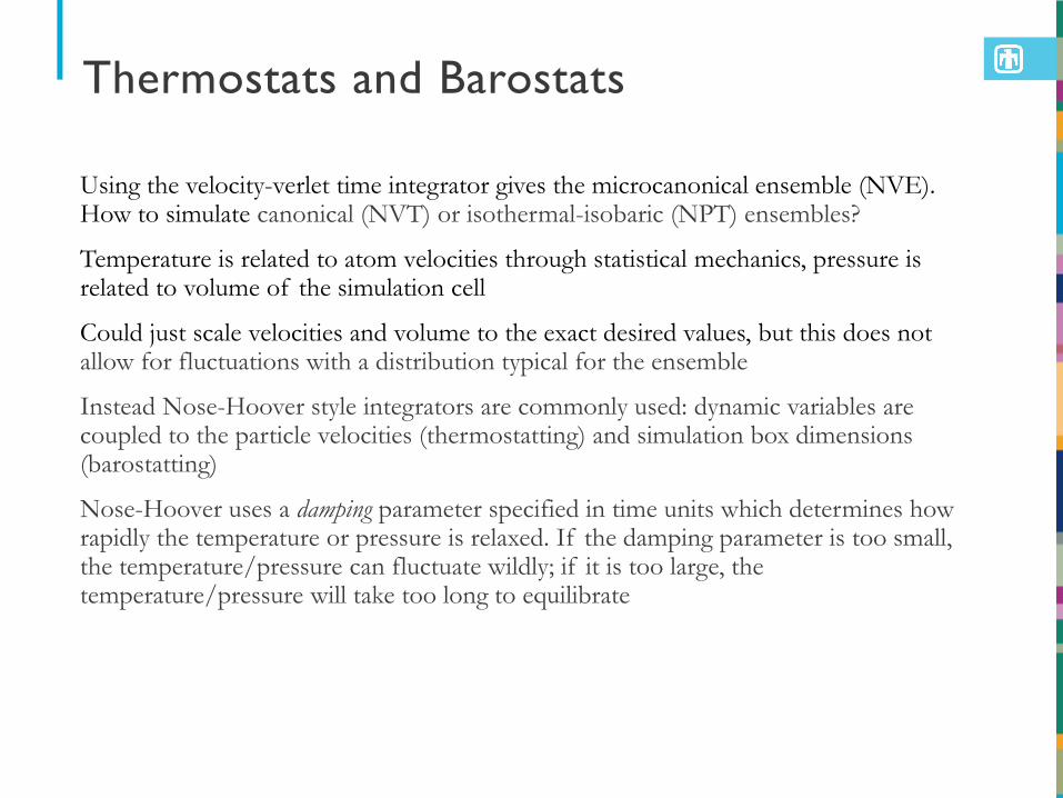
Using the velocity-verlet time integrator gives the microcanonical ensemble (NVE). How to simulate canonical (NVT) or isothermal-isobaric (NPT) ensembles?
Temperature is related to atom velocities through statistical mechanics, pressure is related to volume of the simulation cell
Could just scale velocities and volume to the exact desired values, but this does not allow for fluctuations with a distribution typical for the ensemble
Instead Nose-Hoover style integrators are commonly used: dynamic variables are coupled to the particle velocities (thermostatting) and simulation box dimensions (barostatting)
Nose-Hoover uses a damping parameter specified in time units which determines how rapidly the temperature or pressure is relaxed. If the damping parameter is too small, the temperature/pressure can fluctuate wildly; if it is too large, the temperature/pressure will take too long to equilibrate
Thermostats and Barostats
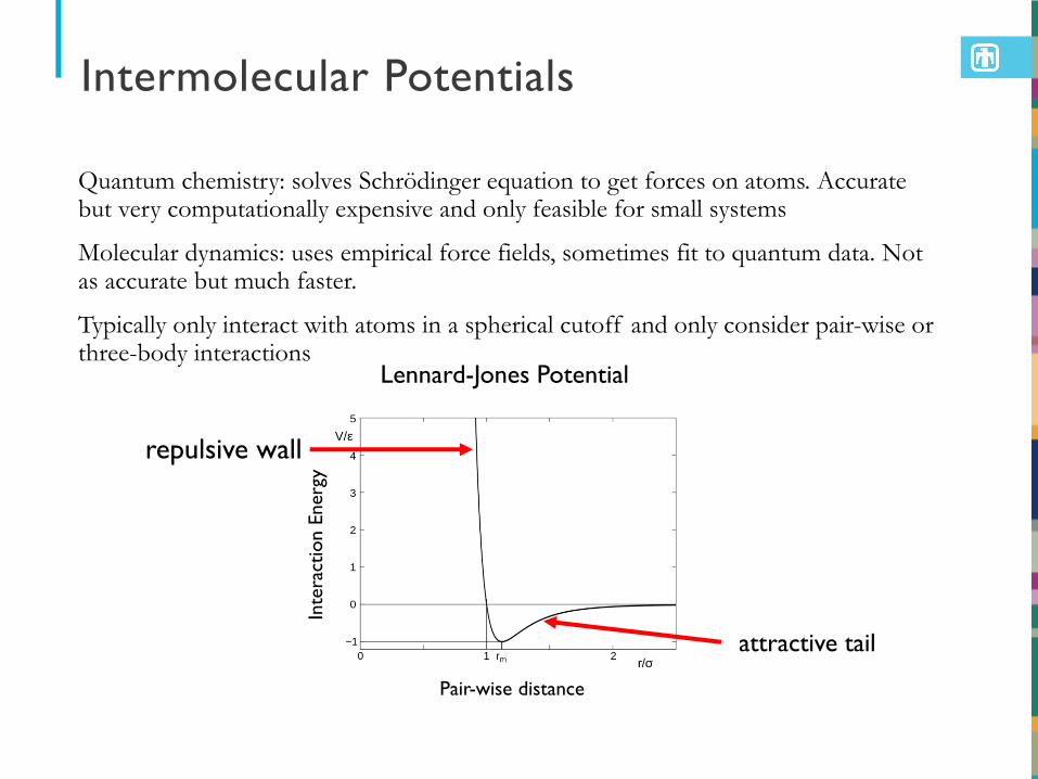
Quantum chemistry: solves Schrödinger equation to get forces on atoms. Accurate but very computationally expensive and only feasible for small systems
Molecular dynamics: uses empirical force fields, sometimes fit to quantum data. Not as accurate but much faster.
Typically only interact with atoms in a spherical cutoff and only consider pair-wise or three-body interactions
Intermolecular Potentials
attractive tail
repulsive wall
Lennard-Jones Potential
Pair-wise distance
Inte
ract
ion E
nerg
y

Interatomic Potentials
LAMMPS Potentials by Material
Biomolecules: CHARMM, AMBER, OPLS, COMPASS (class 2),
long-range Coulombics via PPPM, point dipoles, ...
Polymers: all-atom, united-atom, coarse-grain (bead-spring FENE),
bond-breaking, …
Materials: EAM and MEAM for metals, Buckingham, Morse, Yukawa,
Stillinger-Weber, Tersoff, COMB, SNAP, ...
Chemistry: AI-REBO, REBO, ReaxFF, eFF
Mesoscale: granular, DPD, Gay-Berne, colloidal, peridynamics, DSMC...
Hybrid: can use combinations of potentials for hybrid systems:
water on metal, polymers/semiconductor interface,
colloids in solution, …

More Interatomic Potentials
LAMMPS Potentials by Functional Form
pairwise potentials: Lennard-Jones, Buckingham, ...
charged pairwise potentials: Coulombic, point-dipole
manybody potentials: EAM, Finnis/Sinclair, modified EAM (MEAM), embedded ion
(EIM), Stillinger-Weber, Tersoff, AI-REBO, ReaxFF, COMB
coarse-grained potentials: DPD, GayBerne, ...
mesoscopic potentials: granular, peridynamics
long-range electrostatics: Ewald, PPPM, MSM
implicit solvent potentials: hydrodynamic lubrication, Debye
force-field compatibility with common CHARMM, AMBER, OPLS, GROMACS
options

LAMMPS Potentials
See lammps.sandia.gov/bench.html#potentials
13

Accuracy = Higher Cost14
Moore’s Law for Interatomic PotentialsPlimpton and Thompson, MRS Bulletin (2012).
SNAP
GAPPlimpton and Thompson, MRS Bulletin (2012).

Hybrid force fields
Metal droplet on an LJ surface
◦ metal metal atoms interact with Embedded-Atom potential
◦ surface surface atoms interact with the Lennard-Jones potential
◦ metal/surface interaction is also computed via the Lennard-Jones potential
15
metal
surface

Neighbor ListsNeighbor lists are a list of neighboring atoms within the interaction cutoff + skin for each central atom
Extra skin allows lists to be built less often
16
cutoff

Half Neighbor List
For pair-wise interactions, the force on one atom is equal in magnitude, but opposite in sign, as on the other atom
Can use this principle to reduce computation and the size of the neighbor list (at the cost of more inter-processor communication)
Each pair is stored only once
17

Full Neighbor List
Each pair stored twice, doubles computation but reduces inter-processor communication (can be faster on GPUs)
18

Basic MD Timestep
During each timestep (without neighborlist build):
1. initial integrate
2. compute forces (pair, bonds, etc.)
3. final integrate
4. output (if requested on this timestep)
*Computation of diagnostics (i.e. thermodynamic properties) can be scattered throughout the timestep
19
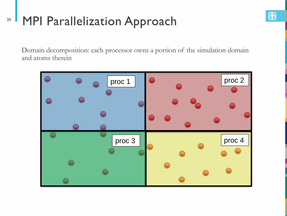
Domain decomposition: each processor owns a portion of the simulation domain and atoms therein
MPI Parallelization Approach20
proc 1 proc 2
proc 3 proc 4

The processor domain is also extended include needed ghost atoms (copies of atoms located on other processors)
Ghost Atoms21
proc 1
local atoms
ghost atoms

Forward communication updates ghost atoms properties (such as positions) from the corresponding real atoms on a different processor
Reverse communication takes properties (such as forces) accumulated on ghost atoms and updates them on the corresponding real atoms on a different processor
Exchange communication migrates real atoms from one processor to another
Border communication creates new ghost atoms
LAMMPS tries to minimize the number of MPI calls required between subdomains
Communication Patterns22

Basic MD Timestep with MPI comm
During each timestep (without neighborlist build):
1. initial integrate
2. MPI forward communication
3. compute forces (pair, bonds, etc.)
4. MPI reverse communication (if newton flag on)
5. final integrate
6. output (if requested on this timestep)
*Computation of diagnostics (fixes or computes) can be scattered throughout the timestep
23

Strong vs Weak Scaling
Strong scaling: hold system size fixed while increasing processor count (# of atoms/processor decreases)
Weak scaling: increase system size in proportion to increasing processor count (# of atoms/processor remains constant)
For perfect strong scaling, doubling the processor count cuts the simulation time in half
For perfect weak scaling, the simulation time stays exactly the same when doubling the processor count
Harder to maintain parallel efficiency with strong scaling because the compute time decreases relative to the communication time
24

Molecular Topology25
Bonds: constrained length between two atoms
Angles: constrained angle between three atoms
Dihedrals: interactions between quadruplets of atoms
Impropers: “improper” interactions between quadruplets of atoms

Long-Range Electrostatics
Truncation doesn’t work well for charged systems due to long-ranged nature of Coulombic interactions
Use Kspace style to add long-range electrostatics:
◦ PPPM—usually fastest, uses FFTs
◦ Ewald—potentially most accurate, but slow for large systems
◦ MSM—multigrid method that also works for non-periodic systems
Usually specify a relative accuracy (1e-4 or 1e-5 typically used)
26

2D Slab Geometry with Kspace
The slab keyword allows a Kspace solver to be used for a systems that are periodic in x,y but non-periodic in z
Must use a boundary setting of “boundary p p f”
Actually treats the system as if it were periodic in z, but inserts empty volume between atom slabs and removing dipole inter-slab interactions so that slab-slab interactions are effectively turned off
May need to use reflecting walls in the z-dimension
27
interfacebulk bulk

Run vs Minimize
“run” command updates velocities and positions based on forces. System may blow up and crash LAMMPS if atoms overlap!
“minimize” command minimizes energy of the system by iteratively adjusting atom coordinates
◦ Good to minimize first if you built your system using an external tool
◦ Prevents LAMMPS crashing from overlapping atoms
Can use “run” after “minimize”
28

Load BalancingAdjusts the size and shape of processor sub-domains within the simulation box
Attempts to balance the number of atoms or particles and thus indirectly the computational cost (load) more evenly across processors
Can be static or dynamic
29
shift
RCB

30
Temperature:
Strain Rate:
• Detailed chemistry is incorporated
in these MD potentials, hot spot
evolution is captured naturally.
• Current capabilities for ReaxFF
within LAMMPS is ~100M
atoms running routinely on
~100k processors
• KOKKOS-Reax/c package
circumvents memory overflow
errors and makes the code portable
to modern architectures (GPU,
KNL, HSW)
APS SCCM Meeting 2017 – Wood, Kittell, Yarrington and Thompson
Shock to Initiation, Deflagration
Example: Energetic Material

Example: Organic Nanowire
This is work by Alexey Shaytan et al. at the Dept of Energy-Related Nanomaterials (University of Ulm, Germany) on a
large-scale fully atomistic MD simulation of the amyloid-like nanofibers formed by the conjugates of oligothiophenes and
oligopeptides. Such compounds are very promising for applications in organic electronics (conductive organic nanowires).
Tranchida

Viscosity for rigid-bodies in SRD fluid32

Triangle and line particle examples33
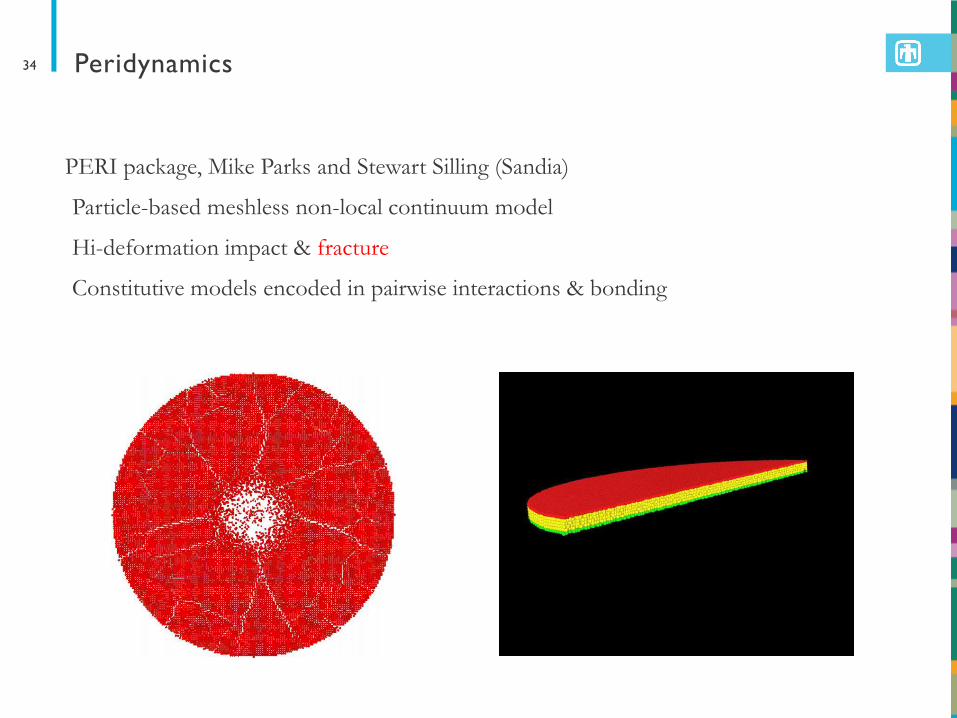
Peridynamics
PERI package, Mike Parks and Stewart Silling (Sandia)
Particle-based meshless non-local continuum model
Hi-deformation impact & fracture
Constitutive models encoded in pairwise interactions & bonding
34

Smoothed particle hydrodynamics
USER-SPH package
Georg Ganzenmüller (Franhofer-Institute, EMI, Germany)
collapse of a water column
35

Granular modeling
GRANULAR package
Christoph Kloss group (JKU) created add-on LIGGGHTS code, (Christoph Kloss now at DCS Computing)
www.cfdem.com
particles + CAD mesh
36

A bit beyond the mesoscale ...
LIGGGHTS code and
FMI (Functional Mock-up Interface) for mesh dynamics
Wheelloader model by C Schubert & T Dresden, (Dresden Tech U)
Simulation by C. Richter & A. Katterfeld, (U Magdeburg OV Guericke)
37
Recommended