Louisiana State UniversityLSU Digital Commons
LSU Master's Theses Graduate School
2014
A Feasibility Study of Ultra-Short Echo Time MRIfor Positive Contrast Visualization of ProstateBrachytherapy Permanent Seed Implants for Post-Implant DosimetryMelissa LambertoLouisiana State University and Agricultural and Mechanical College
Follow this and additional works at: https://digitalcommons.lsu.edu/gradschool_theses
Part of the Physical Sciences and Mathematics Commons
This Thesis is brought to you for free and open access by the Graduate School at LSU Digital Commons. It has been accepted for inclusion in LSUMaster's Theses by an authorized graduate school editor of LSU Digital Commons. For more information, please contact [email protected].
Recommended CitationLamberto, Melissa, "A Feasibility Study of Ultra-Short Echo Time MRI for Positive Contrast Visualization of Prostate BrachytherapyPermanent Seed Implants for Post-Implant Dosimetry" (2014). LSU Master's Theses. 3495.https://digitalcommons.lsu.edu/gradschool_theses/3495

A FEASIBILITY STUDY OF ULTRA-SHORT ECHO TIME MRI
FOR POSITIVE CONTRAST VISUALIZATION
OF PROSTATE BRACHYTHERAPY PERMANENT SEED IMPLANTS
FOR POST-IMPLANT DOSIMETRY
A Thesis
Submitted to the Graduate Faculty of the
Louisiana State University and
Agricultural and Mechanical College
in partial fulfillment of the
requirements for the degree of
Master of Science
in
The Department of Physics and Astronomy
by
Melissa Lamberto
B.S., University of the Sciences in Philadelphia, 2011
August 2014

ii
ACKNOWLEDGMENTS
I thank Dr. Jiang Du for his assistance with the UTE protocol used in this work. I also
thank Randy Deen, MR technologist at PBRC, for his frequent assistance with data collection
and his willingness to lend his knowledge and time.
I express my gratefulness to my advisor, Dr. Kip Matthews, for sharing his expertise and
for his attention to detail each time he reviewed a draft, even at the very last minute. The written
quality of the paper was much improved by his suggestions.
Also, I thank Dr. Guang Jia for his mentorship, for his willingness to send me across the
country to learn new techniques for our research group, for his endless support, and for having
faith in me even when I didn’t! His expertise in the fields of MR physics and image processing
greatly enhanced the quality of this project.
I greatly appreciate Dr. Joe Dugas for his constant clinical support, educational and
personal advice, and his extra participation in the feasibility analysis section. The completion of
this research would be impossible without his extensive involvement. Similarly, I thank Connel
Chu for participating in the feasibility analysis.
I also thank Dr. Sheldon Johnson for his clinical support, especially for taking the time to
further my knowledge of the clinical impact of this study first hand. This project would not exist
without his academic curiosity.
Finally I thank Dr. Les Butler for his contribution to the interpretation of the results from
this study. His eye for detail greatly improved the thoroughness of the analysis component of this
thesis.
All of the faculty of the LSU medical physics program have contributed to the knowledge
necessary to complete this thesis.

iii
TABLE OF CONTENTS
ACKNOWLEDGMENTS .............................................................................................................. ii
LIST OF TABLES ...........................................................................................................................v
LIST OF FIGURES ....................................................................................................................... vi
ABSTRACT .....................................................................................................................................x
CHAPTER 1: INTRODUCTION ....................................................................................................1 1.1 Overview ..............................................................................................................................1 1.2 Current State of Prostate Cancer Treatment ........................................................................1
1.3 Permanent Prostate Brachytherapy ......................................................................................2 1.3.1 Steps of the LDR prostate brachytherapy procedure ..................................................3
1.3.2 Importance of post-implant dosimetry ........................................................................5 1.3.3 Requirements for post implant dosimetry images ......................................................5
1.3.4 Current state of CT for post-implant dosimetry ..........................................................6 1.3.5 Current state of MRI for post-implant dosimetry .......................................................8 1.3.6 Previously published studies using MR-based post-implant dosimetry .....................8
1.3.7 Susceptibility mapping for seed localization ............................................................10 1.4 Goal, Hypothesis, and Aims ..............................................................................................11
CHAPTER 2: BACKGROUND ....................................................................................................13 2.1 Overview ............................................................................................................................13
2.2 MR Physics Review ...........................................................................................................13
2.2.1 T1 relaxation .............................................................................................................14 2.2.2 T2 and T2* relaxation ...............................................................................................15 2.2.3 T1 and T2 for prostate tissue ....................................................................................17
2.3 Pulse Sequence Diagrams and Acquisition Parameters .....................................................17 2.4 Magnetic Susceptibility .....................................................................................................18
2.5 Phase Difference Mapping .................................................................................................19 2.6 Ultra-short Echo Time Pulse Sequence .............................................................................20
2.6.1 Features of UTE pulse sequence ...............................................................................21 2.6.2 Previous studies of UTE imaging of metal ...............................................................21
CHAPTER 3: AIM 1, PHANTOM DEVELOPMENT .................................................................23 3.1 Overview ............................................................................................................................23
3.2 Survey of Material Compositions ......................................................................................23 3.2.1 Target T1 and T2 time constants ..............................................................................23
3.2.2 Recipe and preparation of samples ...........................................................................24 3.2.3 T1 and T2 validation tests .........................................................................................25 3.2.4 T1 and T2 validation results .....................................................................................28
3.3 Pelvic Phantom Fabrication ...............................................................................................29 3.4 Seed Implantation ..............................................................................................................32
3.4.1 Phase maps to assess B0 distortion by titanium seeds...............................................33
iv
3.5 Discussion ..........................................................................................................................35 3.5.1 Seed placement .........................................................................................................35
CHAPTER 4: AIM 2, IMAGE ACQUISITION AND QUALITY ASSESSMENT.....................36
4.1 Overview ............................................................................................................................36 4.2 Materials and Methods .......................................................................................................36
4.2.1 Phantom setup ...........................................................................................................36 4.2.2 UTE acquisition parameters ......................................................................................36 4.2.3 Fast Spin Echo acquisition parameters .....................................................................38
4.3 Results and Discussion ......................................................................................................39 4.3.1 Signal pile-up phenomenon ......................................................................................39 4.3.2 Apparent seed size ....................................................................................................40
4.4 Discussion of UTE Parameter Variations ..........................................................................42
4.4.1 Receiver bandwidth ..................................................................................................42 4.4.2 Flip angle ..................................................................................................................43
4.5 UTE and FSE Comparison.................................................................................................45 4.5.1 Regions of interest ....................................................................................................45
4.5.2 SNR ...........................................................................................................................45 4.5.3 CNR ..........................................................................................................................47 4.5.4 Qualitative assessment ..............................................................................................47
4.5.5 Statistical significance of seed ROI ..........................................................................48
CHAPTER 5: AIM 3, SEED LOCALIZATION PROCEDURE AND RECONSTRUCTION
ACCURACY .....................................................................................................................50 5.1 Overview ............................................................................................................................50
5.2 Materials and Methods .......................................................................................................50
5.2.1 Seed configuration ....................................................................................................50 5.2.2 Characteristics of seed appearance on UTE images .................................................50 5.2.3 Seed counting guidelines ..........................................................................................53
5.3 Results and Discussion ......................................................................................................54 5.3.1 Exclusion of slices at edge of FOV ...........................................................................54
5.3.2 Physicists’ counting results .......................................................................................55 5.4 Discussion ..........................................................................................................................55
5.4.1 Patient scans of UTE without seeds ..........................................................................57
CHAPTER 6: CONCLUSION ......................................................................................................59 6.1 Summary of results ............................................................................................................59 6.2 Response to hypothesis ......................................................................................................59
6.3 Recommendation ...............................................................................................................59 6.4 Limitations of the study .....................................................................................................60
6.5 Future work ........................................................................................................................60
REFERENCES ..............................................................................................................................62
VITA ............................................................................................................................................65

v
LIST OF TABLES
Table 1: Concentrations to produce prostate-like T1 and T2 behavior on a 3T MRI (Hattori
2013). .................................................................................................................................24
Table 2: Parameters used to acquire inversion recovery images to measure the T1 relaxation
time of the phantom materials............................................................................................26
Table 3: Parameters used to acquire spin echo images to measure the T2 relaxation time of the
phantom materials. .............................................................................................................27
Table 4: Concentrations to produce muscle-like T1 and T2 behavior on a 3T MRI (Hattori
2013). .................................................................................................................................30
Table 5: MRI parameters used to collect a UTE image of the pelvic phantom. (Personal
communication with J. Du, UCSD, 2013). ........................................................................37
Table 6: Recommended pulse sequence parameters to collect a T2-weighted image at 3T used
for post-implant dosimetry (Bowes 2013). ........................................................................38
Table 7: Average measured SNR and CNR for both UTE and FSE images. ................................46
Table 8: Results from Student’s t-test performed on the average SNR results for seed prostate
and air signal. .....................................................................................................................49
Table 9: Results of the seed localization test performed by 2 physicists and the author of this
work. ..................................................................................................................................55

vi
LIST OF FIGURES
Figure 1.1: Illustration of prostate anatomy. (top) A sagittal view of the male pelvis with the
prostate highlighted in the red box. (bottom) The enlarged view shows the bladder and
rectum in relation to the healthy prostate (CDC 2013). .......................................................2
Figure 1.2: Photo of a typical brachytherapy seed (Bard Medical, Inc.) used in permanent
prostate brachytherapy. The seed capsule is made of titanium, about 4.5 mm long by 1
mm in diameter as seen on the ruler. ...................................................................................2
Figure 1.3: Illustration of a prostate brachytherapy procedure (Mayo Foundation for Cancer
Research)..............................................................................................................................4
Figure 1.4: CT image of pelvis with seeds implanted into prostate (De Brabandere 2006). ...........7
Figure 1.5: Prostate contours drawn on CT by 7 observers selected for their inexperience in
contouring prostates (De Brabandere 2012). The blue contour was the reference
prostate contour confirmed by two experienced physicists using MRI. The lines shown
in other colors were the contours drawn by the 7 inexperienced observers. .......................7
Figure 1.6: Best (left) and worst (right) case display of seed visibility on MR-based post-
implant dosimetry images (Brown 2013). ...........................................................................8
Figure 1.7: (Left) CT, (middle) T2-weighted MRI, and (right) CT/MR fused post-implant
images of a prostate with contours drawn from the MRI overlaid onto the CT and
CT/MR images. (Brown 2013) ............................................................................................9
Figure 1.8: Axial slice post-implant images of the prostate corresponding to (a) CT, (b) T2-
weighted MRI, and (c) T2*-weighted MRI (Katayama 2011). .........................................10
Figure 2.1: (a) Vector sum of dipole spins along B0, defined as the longitudinal axis, produce
the net magnetization vector, M. (b) At equilibrium, the net magnetization vector
achieves a maximum value, M0. (c) Longitudinal (T1) relaxation of the net
longitudinal magnetization vector; Mz grows exponentially to equilibrium with a time
constant T1 (Hornak 2014). ...............................................................................................14
Figure 2.2: (a) Net magnetization vector rotated into the transverse plane following a 90° RF
pulse. (b) Dephasing of the transverse magnetization. (c) Transverse (T2) relaxation of
the net transverse magnetization vector; Mxy decays exponentially with a time constant
T2 (Hornak 2014). .............................................................................................................15
Figure 2.3: T2 and T2* relaxation of the transverse magnetization vector (Ridgway 2010). .......16
Figure 2.4: Pulse sequence diagram for a gradient recalled echo (Hornak 2014). (a) The RF
pulse perturbs the net magnetization vector (M) from the equilibrium position; the flip
angle, in degrees of rotation from B0, is determined by the strength and duration of the
RF pulse. (b) The slice selection gradient Gs determines the imaging plane and governs
the slice thickness of the image. (c) G is the phase encoding gradient used to alter the

vii
phase angle of the spins as a function of position. (d) Gf is the frequency encoding
gradient which alters the spins’ precession frequency as a function of position
orthogonal to G. The frequency encoding gradient forces an echo to form for signal
collection. (e) S is the echo signal produced by the spins, collected by receiver coils; S
represents the spatial composite of the frequencies and phases of the spins, which is
inverse Fourier transformed into the image. (f) Echo time (TE) is defined as the time
between the center of the RF pulse and the center of the echo. (g) Repetition time (TR)
is the time to complete one full cycle of the pulse sequence. ............................................18
Figure 2.5: Static field (B0) distortion due to the presence of a paramagnetic metallic sphere
(Hornak 2014). ...................................................................................................................19
Figure 2.6: Intensity map and phase map of a metallic sphere in a gelatin phantom (Haacke
1999). In these images, the B0 field points from bottom to top. Distortions in the
intensity map are due to right-left orientation of the frequency-encoding readout
gradient. .............................................................................................................................19
Figure 2.7: Transverse magnetization decay for short T2 and long T2 materials. (top) With a
long TE (conventional MRI), no signal remains from the short T2 material. (bottom)
With a short TE (UTE MRI), signal can be collected from the short T2 material. ...........20
Figure 2.8: (top) Pulse sequence diagrams of a gradient echo pulse sequence that uses (left) a
static orientation of the readout gradients and (right) a 3D radial orientation of the
readout gradients (Bydder 2012). (bottom) Illustration of k-space filling in 2D by each
acquisition method (Hitachi Medical Corporation 2014). .................................................22
Figure 2.9: Observed signal locations (blue, green and black lines) compared to actual signal,
shown as red lines in (a) and (c), of spins adjacent to a 2.5-cm metal block. Signal
pile-up (red arrows) or loss (blue arrows) was seen with shorter or longer echo times
within the UTE sequence (Carl 2013). The red line in (b) illustrates the relative
increase in local magnetic field due to susceptibility. .......................................................22
Figure 3.1: Steps of material preparation. Shown in the top row, (left) digital scale used to
measure chemicals, (center) mixing of chemicals, and (right) heating in a water bath.
Shown in the bottom row, (left) pouring mixture into a mold, (center) a solidified
prostate phantom, and (right) needle insertion into the prostate phantom. ........................25
Figure 3.2: MRmap program used to estimate the T1 relaxation time of the phantom material
(Messroghli 2012). .............................................................................................................27
Figure 3.3: Screenshot of the software program, H.A.N.D, used to measure the T2 relaxation
time of the phantom materials (Hoffman 2012). The first TE was not used for curve
fitting. .................................................................................................................................28
Figure 3.4: Average measured T1 and T2 relaxation times for two prostate phantoms; both of
these samples were used in the pelvic phantom. ................................................................29

viii
Figure 3.5: Creation of pelvic phantom. Three prostates were suspended in the center of the
pelvic phantom (only one is shown in this photo). The spray cans were used to create
voids for possible addition of other tissues. .......................................................................31
Figure 3.6: Pelvic phantom after fabrication was complete but before seed implantation. ...........31
Figure 3.7: Specifications for the BARD brachytherapy seed used to model seed implantation
in this project (Rivard 2004). .............................................................................................32
Figure 3.8: Steps for seed implantation. The seed strands before implantation and the needle
used for seed implantation. ................................................................................................33
Figure 3.9: SourceLink spacers used to space the seeds in different configurations. The seed
spacers were made of 70:30 poly(L-lacgtide-co-D,L-lactide). (BARD Medical) .............33
Figure 3.10: A gradient echo based image (left) and the corresponding phase difference map
(right) of the pelvic phantom after the seeds were implanted. ...........................................34
Figure 4.1: Illustration of the phantom setup in the MRI scanner. ................................................37
Figure 4.2: Illustration of the signal pile-up effect where signal is shifted spatially to a falsely
represented location in the spatial position image (Bydder 2012). ....................................39
Figure 4.3: Sagittal view of 3 seeds from two trials of UTE acquisition, with (top) 20 cm FOV
compared to (bottom) 18 cm FOV. The cartoons illustrate where the pile up occurred
relative to the centers of the seeds. ....................................................................................40
Figure 4.4: Line profile measurements measured in ImageJ (Rasband 1997) for the same slice
in both UTE and FSE images. The line profiles plot pixel intensity along the blue line
in each image. ....................................................................................................................41
Figure 4.5: Line profiles for the same seed from both FSE and UTE displayed on the same
scale. This graph illustrates the ability of UTE to capture the large signal magnitude
due to pile-up. ....................................................................................................................42
Figure 4.6: Three different receiver bandwidths used to acquire the same image slice with
UTE. Note how the appearance of the bright ring (pile-up artifact) around a seed
decreases with increasing bandwidth. ................................................................................43
Figure 4.7: Three different flip angles used to acquire the same image slice with UTE. ..............44
Figure 4.8: Relative transverse signal intensity as a function of flip angle. The Ernst angle is
flip angle where the signal intensity is highest. .................................................................45
Figure 4.9: Samples of the regions of interest drawn with ImageJ (Rasband 1997) to collect
signal intensities and standard deviation. These values were used to calculate SNR and
CNR. ..................................................................................................................................46

ix
Figure 4.10: Gradient-recalled echo images a) with TE: 2.25 ms and b) TE: 5.8 ms and all
other parameters held constant of the same slice in the pelvic phantom. Phase
difference map c) of the same slice. This map was collected using concepts discussed
in section 2.5. Corresponding d) FSE and e) UTE images of the same slice in the
pelvic phantom. ..................................................................................................................48
Figure 4.11: A seed (white arrow) on 8 consecutive slices (0.7013 mm thick). The red arrow
shows where the pile-up in the center of the ring that is used to identify the presence of
a seed on the UTE image. ..................................................................................................49
Figure 4.12: An air bubble (white arrow) on 4 consecutive slices (0.7013 mm thick). This
shows the lack of bright center that the seed characteristically displays on the same
scan. ...................................................................................................................................49
Figure 5.1: Seed configurations implanted. The varied configuration (top) was used to test the
seed localization accuracy and the standard configuration (bottom) was used for
reference. ............................................................................................................................51
Figure 5.2: Comparative orthogonal views of the same location on both UTE and FSE images.
The spacing between the beginning of two seed strands (1) is almost double the
spacing towards the end of the same two seed strands (2) as highlighted in the Coronal
UTE image .........................................................................................................................51
Figure 5.3: An illustration used to explain how a seed will appear to observers in UTE images.
The dark black arrow on the right of the illustration shows how the slices would be
scrolled through in the axial direction. ..............................................................................52
Figure 5.4: Description (right) of what is visible on a sample UTE slice (left) shown to
observers as training for seed counting. .............................................................................52
Figure 5.5: Axial view of seed on UTE image. The yellow cursor is centered on the seed by
the observer. .......................................................................................................................53
Figure 5.6: The corresponding coronal (left) and sagittal (right) views of the seed centered in
Figure 5.5. ..........................................................................................................................53
Figure 5.7: Area of elevated signal intensity due to the contamination of ultra-short T2 signal
from the polycarbonate walls of the pelvic phantom. The outlined areas (labeled “Area
of Failure”) were excluded in the localization tests ...........................................................54
Figure 5.8: A selected slice with poor prostate definition on the UTE image (left) and slightly
improved prostate definition on the corresponding FSE image (right). ............................56
Figure 5.9: UTE scans of the prostate of a healthy volunteer. The top image shows contours of
the prostate, bladder and rectum for the same patient in the bottom images. ....................58

x
ABSTRACT
Ultra-short echo time (UTE) imaging is a magnetic resonance imaging (MRI) technique
that uses very short echo times (on the order of microseconds) to measure rapid T2 relaxation.
An application of UTE is the visualization of magnetic susceptibility-induced shortening of T2 in
tissues adjacent to metal, such as prostate tissue with implanted brachytherapy seeds. This study
assessed UTE imaging of prostate brachytherapy seeds on a clinical 3T MRI scanner to provide
images for post-implant dosimetry.
A prostate tissue phantom was made of gelatin mixed with Gd and other materials to
mimic the prostate peripheral zone’s T1 and T2 relaxation times; this phantom was used to
investigate the effect of UTE acquisition parameters on brachytherapy seed visibility. A second
phantom was made to model prostate tissue surrounded by muscle tissue; this pelvic phantom
was implanted with 85 titanium brachytherapy seeds (STM1251, Bard Medical). Both phantoms
were scanned on a 3T GE scanner with a 3D UTE pulse sequence and a fast spin echo (FSE)
pulse sequence. The average seed SNR, the CNR between seed and prostate material, and visual
characteristics of the seeds were assessed. A seed counting procedure was developed based on
the visual seed characteristics, and subsequently used by two physicists to locate seeds in UTE
images of the pelvic phantom.
On 3D UTE images, the metal seeds caused a bright ring-link artifact in adjacent prostate
tissue due to susceptibility-induced T2 shortening. The average seed SNR was 15.99±1.52 for
UTE compared to 32.32±22.43 for FSE; CNR between seed and prostate was 6.73±1.85 for UTE
vs. 23.76±12.87 for FSE. The ring was larger in diameter than a seed itself; apparent seed
diameters were 4.65±0.363 mm for UTE compared to 1.46±0.38 mm for FSE. The 3D spatial
ring pattern facilitated differentiation of seeds from needle tracks and seed spacers. The two

xi
physicists counted 83 and 86 seeds respectively in the UTE images. Prostate boundaries were
less well visualized with UTE compared to FSE.
With its ability to visualize brachytherapy seeds, UTE imaging appears to provide an
alternative approach to CT for seed identification. Compared to fusion of separately-acquired CT
images and T2-weighted MR images (for delineation of prostate boundaries), UTE and T2-
weighted MR can be acquired in a single imaging session – a convenience to patients while
potentially minimizing inter-modality image registration issues. A study in prostate
brachytherapy patients of the quality of post-implant dosimetry with UTE imaging compared to
CT imaging is recommended.

1
CHAPTER 1: INTRODUCTION
1.1 Overview
The goal of this project was to investigate the feasibility of an ultra-short echo time
(UTE) magnetic resonance imaging (MRI) pulse sequence for localization of permanent
brachytherapy seeds. UTE is a pulse sequence that provides a unique perspective on imaging
seeds after implantation due to the positive contrast of metal compared to tissue in UTE images.
This thesis summarizes the theory of UTE and the artifacts produced when metallic objects are
imaged. Possible limitations inherent in the UTE technique are discussed. This project utilized
phantom studies to evaluate the possibility of implementing UTE for post-implant seed
localization in clinical practice for prostate brachytherapy.
1.2 Current State of Prostate Cancer Treatment
The prostate is a male genitourinary gland located in the pelvis (Figure 1.1). According to
the 2012 SEER report, one in seven American men will be diagnosed with prostate cancer in his
lifetime; prostate cancer is the second most common cancer among men in the United States
after skin cancer (Howlader 2013). There are various treatment options for these men depending
on the extent of their cancer at presentation.
Of the men diagnosed with prostate cancer annually, 81% have disease that is confined
within the prostate capsule (Howlader 2013). Permanent prostate brachytherapy (PPB)
monotherapy is suggested as a standard-of-care treatment option for these low-risk (Gleason
3+3, PSA <10 and T1c or T2a) patients (Davis 2012). Low intermediate risk (usually only one
of: Gleason 3+4, PSA 10-20, T2b or T2c) patients are regarded by many physicians as
candidates for monotherapy. Higher risk patients may be candidates for PPB implant as a boost
with external beam radiotherapy.

2
Figure 1.1: Illustration of prostate anatomy. (top) A sagittal view of the male pelvis with the
prostate highlighted in the red box. (bottom) The enlarged view shows the bladder
and rectum in relation to the healthy prostate (CDC 2013).
1.3 Permanent Prostate Brachytherapy
Permanent prostate brachytherapy is low dose rate, “sealed-source” radiotherapy. It is a
cancer treatment technique that requires a physician to implant radioactive, cylindrical sources,
called seeds (Figure 1.2), into the patient’s prostate. The seeds remain in the patient indefinitely.
Figure 1.2: Photo of a typical brachytherapy seed (Bard Medical, Inc.) used in permanent
prostate brachytherapy. The seed capsule is made of titanium, about 4.5 mm long by
1 mm in diameter as seen on the ruler.
Low dose rate radioactive materials commonly used for this procedure are iodine-125 and
palladium-103. Different designs are available from the various manufacturers (see Section 3.2.4

3
for a discussion of the design used in this project). Implantation of these seeds into the prostate is
planned so that a prescribed therapeutic dose is delivered to the prostate itself while dose to the
surrounding tissues, i.e. rectum and bladder, is minimized.
1.3.1 Steps of the LDR prostate brachytherapy procedure
A typical prostate brachytherapy procedure is completed in three steps: (1) pre-treatment
planning, (2) implantation of radioactive seed sources, and (3) evaluation of the quality of the
implant. Each part of this process relies heavily on imaging to ensure a quality procedure that
delivers the desired dose.
In the first step, the prostate is imaged with trans-rectal ultrasound (TRUS) and a pre-plan
is generated. The physician contours the prostate as well as the organs at risk, which include the
urethra, bladder, and rectum. For monotherapy PPB, the typical prescribed dose is 125-145 Gy
depending on the selected radioactive source. The dosimetrist or physicist maps out where the
seeds should be placed to achieve the best possible dose coverage of the prostate while
minimizing the dose to the rectum, bladder, and urethra. As recommended by the American
Brachytherapy Society, the entire prostate volume must be covered by 100% of the prescribed
dose, while the urethra should not exceed 150% of the prescribed dose (Nag 2000, Tempany
2012).To achieve the desired dose coverage, seeds are usually placed peripherally in the prostate
to maximize the dose to the whole gland while minimizing the dose to the centrally located
urethra. The plan ideally limits dose to the rectum and bladder immediately adjacent to the
prostate. This pre-plan determines the number of seeds needed for a successful implant;
typically, around 100 seeds are implanted within a 40-60 cc prostate.
In the second step, the physician implants the seeds by hand using TRUS image guidance
(Figure 1.3). Seeds are loaded in needles for implantation. A typical implant uses about 20

4
needles and takes approximately 1-2 hours in an outpatient setting. When estimating the dose
coverage, the physician must consider error associated with the hand placement technique. Many
physicians overestimate the dose coverage by about 2 mm outside of the entire prostate
(Tempany 2012). Also, the prostate swells due to the needle insertions which may cause
movement of seeds after placement in the prostate.
Figure 1.3: Illustration of a prostate brachytherapy procedure (Mayo Foundation for Cancer
Research).
In the final step of the process, the patient returns for a follow-up visit approximately 30
days after implantation, which allows time for swelling to abate. This part of the procedure,
called post-implant dosimetry, is typically performed with computed tomography (CT) images.
The pelvis is imaged, the seed locations are identified, and the delivered dose is re-calculated

5
according to the seed positions relative to the prostate contour. This post-plan is used by the
physician to assess plan quality and overall success. Furthermore, if the delivered dose is
insufficient, supplemental treatment options can be recommended.
1.3.2 Importance of post-implant dosimetry
Considering the errors possible from the hand delivery technique, re-calculating the
delivered dose is crucial to estimate actual dose coverage. While the main purpose of post-
implant dosimetry is to assess the quality of the delivered plan, it also provides quality assurance
for future implant procedures by helping the physician improve his or her technique. With high
quality post-implant dosimetry, physicians can analyze the procedures to determine correlations
between treatment delivery, patient morbidity, and tumor control.
1.3.3 Requirements for post implant dosimetry images
Post-implant dosimetry is a critical step in the brachytherapy process, but currently has
several shortcomings which lead to uncertainty in treatment outcomes. Current brachytherapy
treatment guidelines mandate the use of an acceptable imaging modality for seed localization and
prostate delineation for post-implant dosimetry calculations. CT is the common modality,
currently. For post-implant images to be clinically useful, the image must:
(1)show the locations of the implanted seeds;
(2)show the outline of the prostate for calculations; and
(3)provide a realistic representation of the internal anatomy (with minimal spatial distortions)
Fortunately, post-implant dosimetry uses a dose calculation formalism that does not
require electron density to determine delivered dose (Rivard 2004). Unlike the majority of
radiation planning scenarios, brachytherapy delivers dose at short range to tissues with similar
electron densities. According to the Task Group 43 guidelines from the American Association of

6
Physicists in Medicine (Nath 1994), the delivered dose is determined by approximating the tissue
density to be water-equivalent throughout the patient. Essentially all tissue inhomogeneities can
be ignored (Rivard 2004).This means that a variety of imaging modalities, besides CT, could be
used for dose calculation, as long as that image source provides accurate locations of the seeds
with respect to the prostate volume. Determining a true prostate outline provides a precise
treatment evaluation which, as discussed previously, should lead to improvements in future
treatment accuracy and aid in prediction of side effects from the procedure.
1.3.4 Current state of CT for post-implant dosimetry
Although the recommended treatment guidelines state that CT is a useful modality for
post-implant dosimetry calculations, poor visibility of both prostate and seeds on a CT image
causes uncertainty in the re-calculated delivered dose (Lindsay 2003, Crook 2010). One issue
that occurs with CT imaging is the presence of streaking artifacts due to the high Z material of
the seed (Figure 1.4). This leads to artifacts on the post-implant image which degrade the
accuracy of dosimetry calculations (Dubois 2001, Lindsay 2003).
Published studies show that using CT images for post-implant dosimetry often lead to
overestimation of the prostate volume due to the physician’s disrupted view of the prostate from
seed artifacts (Bowes 2013). Additionally, inter-observer variability increases when prostate
volumes are contoured on CT images (De Brabandere 2012). This is illustrated in Figure 1.5,
where 3 prostates were contoured by 7 inexperienced physicists on selected CT slices, as
compared to the reference prostate contour delineated by two experienced physicists.

7
Figure 1.4: CT image of pelvis with seeds implanted into prostate (De Brabandere 2006).
Figure 1.5: Prostate contours drawn on CT by 7 observers selected for their inexperience in
contouring prostates (De Brabandere 2012). The blue contour was the reference
prostate contour confirmed by two experienced physicists using MRI. The lines
shown in other colors were the contours drawn by the 7 inexperienced observers.
8
1.3.5 Current state of MRI for post-implant dosimetry
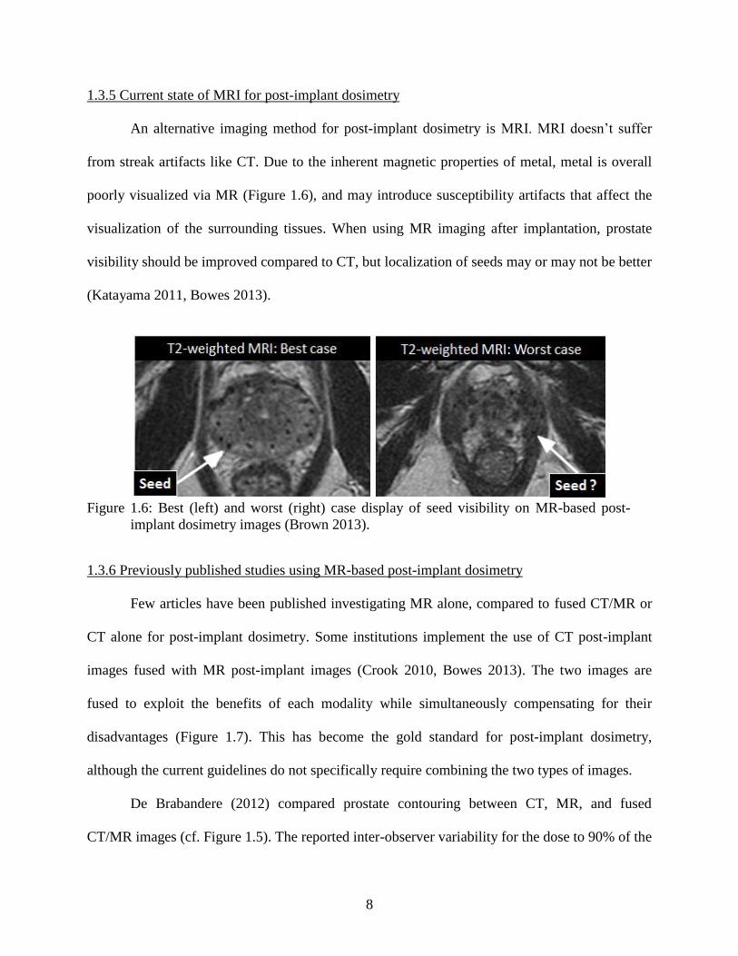
An alternative imaging method for post-implant dosimetry is MRI. MRI doesn’t suffer
from streak artifacts like CT. Due to the inherent magnetic properties of metal, metal is overall
poorly visualized via MR (Figure 1.6), and may introduce susceptibility artifacts that affect the
visualization of the surrounding tissues. When using MR imaging after implantation, prostate
visibility should be improved compared to CT, but localization of seeds may or may not be better
(Katayama 2011, Bowes 2013).
Figure 1.6: Best (left) and worst (right) case display of seed visibility on MR-based post-
implant dosimetry images (Brown 2013).
1.3.6 Previously published studies using MR-based post-implant dosimetry
Few articles have been published investigating MR alone, compared to fused CT/MR or
CT alone for post-implant dosimetry. Some institutions implement the use of CT post-implant
images fused with MR post-implant images (Crook 2010, Bowes 2013). The two images are
fused to exploit the benefits of each modality while simultaneously compensating for their
disadvantages (Figure 1.7). This has become the gold standard for post-implant dosimetry,
although the current guidelines do not specifically require combining the two types of images.
De Brabandere (2012) compared prostate contouring between CT, MR, and fused
CT/MR images (cf. Figure 1.5). The reported inter-observer variability for the dose to 90% of the

9
contoured prostate volume (D90) based on seed localization from the CT image was 2%
variation, while the D90 varied by 7% for the use of MR-based seed localization. In the image
fusion-based localization study, the D90 varied by 2% as well.
Figure 1.7: (Left) CT, (middle) T2-weighted MRI, and (right) CT/MR fused post-implant
images of a prostate with contours drawn from the MRI overlaid onto the CT and
CT/MR images. (Brown 2013)
Unfortunately, MR/CT fusion can be difficult, due to distortion of the MR images from
various factors. Also, obtaining both types of images may be impractical for some facilities. For
example, an MRI scanner may not be available onsite; off-site MR imaging would require a
separate patient appointment. From a patient’s perspective, convenience dictates using a single
imaging modality for post-implant dosimetry. MR imaging provides good visualization of the
prostate, but using it to visualize seeds is an area needing further exploration.
Tanaka et al (2006) investigated the use of T2, T1, contrast enhanced, and fat suppressed
T1 images. They concluded that MR-based dosimetry was adequate for prostate contouring, but
seed localization was inadequate. Other authors investigated the possibility of fusing T2-
weighted and T2*-weighted MR images (Figure 1.8) to create a final post-implant dosimetry
image (Katayama 2011). The main error discovered by this technique involved the localization
of seeds outside of the prostate within the pelvis (cf. Figure 1.6). The seeds were difficult to
visualize due to the fact that inherent inhomogeneities in the pelvic region appear similar on MR

10
image to those introduced by the seeds. These inhomogeneities included hemorrhages,
calcifications, blood vessels, and air bubbles. The results suggested that MR-based dosimetry is
possible, but a better pulse sequence may be necessary to extract the seed locations from the MR
image.
Figure 1.8: Axial slice post-implant images of the prostate corresponding to (a) CT, (b) T2-
weighted MRI, and (c) T2*-weighted MRI (Katayama 2011).
1.3.7 Susceptibility mapping for seed localization
A pulse sequence that could lead to improved seed detection is susceptibility mapping.
(Chapter 2 provides a review of MR physics including the concept of susceptibility). The
magnetic susceptibility of the metal seeds alters local magnetic field strength; adjacent tissues
exhibit a different resonance behavior than distant tissues. Specifically, the metal seeds cause a
spatial variability in the local tissue relaxation rates (Haacke 1999). This phenomenon can be
exploited with a type of image sequence called susceptibility mapping. Susceptibility mapping
identifies metallic objects by mapping out the magnetic field changes due to the metal. Ideally,
non-metallic objects don’t alter susceptibility so only the location of the metal seeds would be
identified.

11
Susceptibility mapping can be further enhanced to achieve visual seed distinction, called
positive contrast. Essentially, the protons that produce an on-resonance signal (e.g., those from
non-metal material) are suppressed. The scanner only reads the signals that occur off-resonance,
at a shifted frequency that corresponds to the altered local magnetic field strength in the vicinity
of the metal seeds. One group has published promising phantom results that show this concept is
feasible to locate seeds within the prostate area (Kuo 2010). Extra-prostatic inhomogeneities
were ignored in this study.
1.4 Goal, Hypothesis, and Aims
The goal of this project was to identify and assess an MRI pulse sequence that could
distinguish permanently implanted prostate brachytherapy seeds from their surroundings. An
ideal sequence would visualize all seeds, i.e. with high contrast vs. prostate, and would allow the
seeds to be differentiated from air cavities or other confounding structures. An ideal sequence
also would be able either to visualize the prostate boundaries within the pelvis or to have
minimal spatial distortions to facilitate registration with other MRI scans or CT.
We hypothesized that a 3D ultra-short echo time (UTE) pulse sequence will provide MR
images of permanent brachytherapy seeds with positive contrast, defined as seed signal that is
statistically larger than the prostate signal (p<0.05). The seeds also will be distinguishable from
air on the UTE images, meaning the signal from metal will have a signal that is statistically
different than the signal from air cavities within the prostate (p<0.05).
This project was executed through the completion of three aims. The following chapters
provide a review of MR imaging concepts, including the UTE pulse sequence, and address the
approach and results for each aim.

12
Aim 1, Phantom Development: Develop a phantom with magnetic resonance behavior that
models human prostate tissue at 3T, which can be implanted with brachytherapy seeds.
Aim 2, Image Acquisition and Quality Assessment: Acquire images with a selection of 3D UTE
pulse sequence parameters that provide positive seed contrast. Analyze these images for
several image quality metrics.
Aim 3, Seed Localization Procedure and Reconstruction Accuracy: Create a procedure for
identifying the locations of seeds in UTE images. Have two physicists use the procedure
to identify and locate seeds in a pelvis phantom.

13
CHAPTER 2: BACKGROUND
2.1 Overview
This chapter reviews concepts about magnetic resonance imaging that are relevant to an
understanding of this thesis.
2.2 MR Physics Review
Magnetic resonance imaging (MRI) is a non-invasive imaging technique that exploits the
nuclear magnetic resonance behavior of atoms to gain spatial information about their
environment. Nucleons (protons and neutrons) possess spin angular momentum, giving each a
magnetic moment. Atoms with an odd atomic mass, like hydrogen, possess a non-zero net
nuclear magnetic moment, generically called a “spin”. When placed in an external magnetic field
of strength B0, the spins precess at the Larmor frequency, , as
(2.1)
The gyromagnetic ratio, , is a constant that is characteristic of the atom; typical units are
MHz/T. The external or static B0 field is generated by the MRI scanner. While in the static field,
each hydrogen spin acts as a dipole magnet. Each spin occupies either a low energy “spin-up”
state (when the dipole aligns with B0) or a high energy “spin-down” state (when the dipole aligns
opposite to B0). The vector sum of the diploes along B0 (designated as the longitudinal axis) is
the net longitudinal magnetization vector, Mz, illustrated in Figure 2.1a (Hornak 2014). At
equilibrium (Figure 2.1b), this net magnetization vector reaches a maximum value, M0,
indicating the largest possible number of spins are located in the spin-up state.
In a magnetic field, the spins in different materials behave in unique ways. For instance,
fat appears different than cartilage or muscle due to differing degrees of spin interactions in these
tissues. To collect information about the environment of the spins, a radiofrequency (RF) pulse is

14
applied to the imaging volume to perturb the dipole moments, effectively pushing their
alignment away from B0. After the RF pulse, the net magnetization vector returns over time to
the equilibrium state (Figure 2.1c). The rate of return is determined by the interactions of the
spins with each other and with the local molecular environment. The interactions are exponential
processes characterized by tissue-specific time constants.
(a) (b)
(c)
Figure 2.1: (a) Vector sum of dipole spins along B0, defined as the longitudinal axis, produce
the net magnetization vector, M. (b) At equilibrium, the net magnetization vector
achieves a maximum value, M0. (c) Longitudinal (T1) relaxation of the net
longitudinal magnetization vector; Mz grows exponentially to equilibrium with a time
constant T1 (Hornak 2014).
2.2.1 T1 relaxation
Spin-lattice relaxation describes the rate at which the longitudinal magnetization vector
re-grows over time (Figure 2.1c), given by
( ) (
) (2.2).
15
where T1 is the spin-lattice relaxation time constant, M0 is the equilibrium magnitude, and t is
the time since the perturbation by the RF pulse. T1 relaxation occurs as spins exchange energy
with the environment (lattice) to move from the spin-down state to the spin-up state.
2.2.2 T2 and T2* relaxation
The magnitude and duration of the perturbing RF pulse determines the amount by which
the net magnetization vector is pushed away from the longitudinal axis, typically expressed in
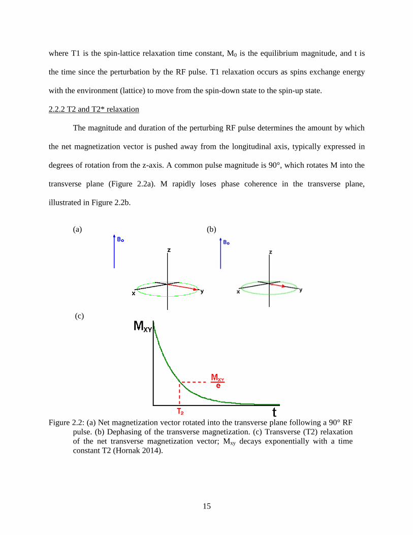
degrees of rotation from the z-axis. A common pulse magnitude is 90°, which rotates M into the
transverse plane (Figure 2.2a). M rapidly loses phase coherence in the transverse plane,
illustrated in Figure 2.2b.
(a) (b)
(c)
Figure 2.2: (a) Net magnetization vector rotated into the transverse plane following a 90° RF
pulse. (b) Dephasing of the transverse magnetization. (c) Transverse (T2) relaxation
of the net transverse magnetization vector; Mxy decays exponentially with a time
constant T2 (Hornak 2014).

16
The T2 time constant represents the rate of decay of the transverse magnetization vector
due to phase loss during spin-spin interactions. Also termed spin-spin relaxation, T2 relaxation is
illustrated in Figure 2.2c and described by
( ) ( ) (2.3)
where Mxy(0) is the magnitude of the net magnetization in the transverse plane, immediately after
the RF pulse has been applied, and T2 is the spin-spin relaxation time constant.
A second contributor to the loss of transverse magnetization is T2* decay, which
represents loss of phase coherence of the spins due to inhomogeneities in the B0 field (Figure
2.2b). The T2* time constant folds together the T2 and inhomogeneity relaxation effects as
(2.4)
where B0 represents the magnitude of B0 field inhomogeneity. Large inhomogeneities result in
short T2*, masking the T2 relaxation of the spins. This results in a rapidly disappearing signal
that may cause signal collection difficulties (Figure 2.3).
Figure 2.3: T2 and T2* relaxation of the transverse magnetization vector (Ridgway 2010).

17
2.2.3 T1 and T2 for prostate tissue
The T1 and T2 relaxation rates are unique to a specific tissue when placed in a magnetic
field, although T1 depends on B0 while T2 does not. The time constants for prostate tissue at 3T
are approximately T1=1597 ms and T2=74 ms (Hattori 2013). The T2 relaxation rate varies
depending on the location of the prostate tissue within the whole gland: central gland T2=78 ± 8
ms, peripheral zone T2=114 ± 27 ms, tumor T2=82 ± 15 ms (Foltz 2013). The relaxation time
constants for a material are determined by measuring signal intensity at various points in time.
2.3 Pulse Sequence Diagrams and Acquisition Parameters
A pulse sequence diagram describes the series of events that occur during an MRI scan.
A gradient recalled echo pulse sequence diagram is shown in Figure 2.4. When collecting a
signal, the user defines the acquisition parameters of the pulse sequence to emphasize a
particular component of relaxation. User-defined variables include echo time (TE), repetition
time (TR), slice thickness, flip angle, receiver bandwidth, field of view, pixel size, frequency
encoding gradient, phase encoding gradient, step sizes, direction, and number of measurements
or excitations per voxel. These parameters are discussed when appropriate in the following
sections, in addition to the following definitions:
a) Field of view (FOV) is the distance across the image in the frequency encoding direction.
b) Receiver bandwidth (rBW) is the range of frequencies accepted by the receiver coil.
c) Flip angle is the angle by which the net magnetization vector (M0) is rotated or perturbed
from the longitudinal axis.
d) K-space is the coordinate space covered by the phase and frequency encoding gradient data;
k-space is the Fourier transform of image space.

18
(a)
(b)
(c)
(d)
(e)
(f)
(g)
Figure 2.4: Pulse sequence diagram for a gradient recalled echo (Hornak 2014). (a) The RF
pulse perturbs the net magnetization vector (M) from the equilibrium position; the flip
angle, in degrees of rotation from B0, is determined by the strength and duration of
the RF pulse. (b) The slice selection gradient Gs determines the imaging plane and
governs the slice thickness of the image. (c) G is the phase encoding gradient used to
alter the phase angle of the spins as a function of position. (d) Gf is the frequency
encoding gradient which alters the spins’ precession frequency as a function of
position orthogonal to G. The frequency encoding gradient forces an echo to form
for signal collection. (e) S is the echo signal produced by the spins, collected by
receiver coils; S represents the spatial composite of the frequencies and phases of the
spins, which is inverse Fourier transformed into the image. (f) Echo time (TE) is
defined as the time between the center of the RF pulse and the center of the echo. (g)
Repetition time (TR) is the time to complete one full cycle of the pulse sequence.
e) Number of excitations (NEX) determines the number of times each line of k-space is
sampled; NEX is the number of repeat measurements used to decrease image noise.
2.4 Magnetic Susceptibility
Magnetic susceptibility is the ability of a metal to become magnetized when placed in a
magnetic field. Highly susceptible ferromagnetic materials interact strongly with external
magnetic fields. Ferromagnetic metals become magnetized because of their large susceptibility
and may exhibit permanent magnetization; ferromagnetic materials are unsafe for MRI. Because
of their weak susceptibility, paramagnetic materials and diamagnetic materials are only slightly
magnetized compared to ferromagnets. Paramagnetic and diamagnetic metals do not remain
magnetized when removed from the external magnetic field. Both types of materials alter the

19
external magnetic field in their vicinity (Figure 2.5); paramagnetic metals such as titanium
concentrate the magnetic field lines in their vicinity.
Figure 2.5: Static field (B0) distortion due to the presence of a paramagnetic metallic sphere
(Hornak 2014).
2.5 Phase Difference Mapping
Phase difference maps (Figure 2.6) are a convenient way to visualize the B0 distortions
caused by the presence of paramagnets in a magnetic field. The values in the phase map
represent frequency differences from the Larmor frequency (ω0); frequencies higher or lower
than ω0 are due to relatively increased or decreased local magnetic field strength, respectively.
The apparent abrupt transitions (from dark to bright) in the phase map, called phase wrapping,
are because frequency shifts have a period of 2. The phase differences reveal information about
B0 inhomogeneities because of its effect on T2* relaxation.
Figure 2.6: Intensity map and phase map of a metallic sphere in a gelatin phantom (Haacke
1999). In these images, the B0 field points from bottom to top. Distortions in the
intensity map are due to right-left orientation of the frequency-encoding readout
gradient.

20
2.6 Ultra-short Echo Time Pulse Sequence
Tissues with a short T2 time constant lose their signal rapidly; additional T2* shortening
further increases the rate of signal loss. Figure 2.7 compares the magnitudes of transverse signal
over time for short T2 and long T2 materials. If the acquisition TE is long compared to the short
T2 (or T2*), as in Figure 2.7(top), the signal from the short T2 material will be completely
decayed by the time of signal acquisition. This material will not appear in the collected image.
Using a shorter TE allows the signal from rapidly decaying tissues to be collected and therefore
represented on the MR image, as shown in Figure 2.7 (bottom).
Figure 2.7: Transverse magnetization decay for short T2 and long T2 materials. (top) With a
long TE (conventional MRI), no signal remains from the short T2 material. (bottom)
With a short TE (UTE MRI), signal can be collected from the short T2 material.

21
A reduction of TE imposes critical restrictions on the pulse sequence parameters, such as
limiting the flip angle (with short RF flip pulses) or using separate coils for RF generation and
signal reception. The main feature of the UTE pulse sequence is the ability to collect a signal
about 1 order of magnitude faster than the fastest TE available on conventional MRI scanners
(Robson 2003, Bydder 2012).
2.6.1 Features of UTE pulse sequence
Extremely short TE acquisition imposes restrictions on the pulse sequence parameters.
These parameters influence image quality and overall imaging time, as well as pushing the limits
of the scanner hardware. The UTE pulse sequence investigated in this project was a 3-
dimensional scan. The 3D UTE scan produces isotropic resolution. This is advantageous to
localize fine details on an image, e.g., titanium seeds for the current project.
The UTE sequence uses radial filling of k-space to achieve isotropic resolution and rapid
acquisitions (Figure 2.8). With radial acquisition, the spatial encoding gradients rotate in
orientation relative to the coordinate system of the image slice. This results in susceptibility
artifacts with radial symmetry rather than the left-right symmetry shown in the phase map of
Figure 2.6 where the readout direction was only in the horizontal direction. This has implications
for the appearance of brachytherapy seeds, as discussed in section 5.2.2.
2.6.2 Previous studies of UTE imaging of metal
A study by Carl et al. (2013) highlighted the ability of the UTE sequence to preserve
signal from tissue adjacent to metal that would otherwise be lost from rapid T2* de-phasing of
the transverse signal. An interesting characteristic was noted when ultra-short echo times were
used for signal acquisition. Very short TE caused a large displacement of signal (red arrows in
Figure 2.9) while a longer TE caused a loss of signal (blue arrows) at the boundary of two
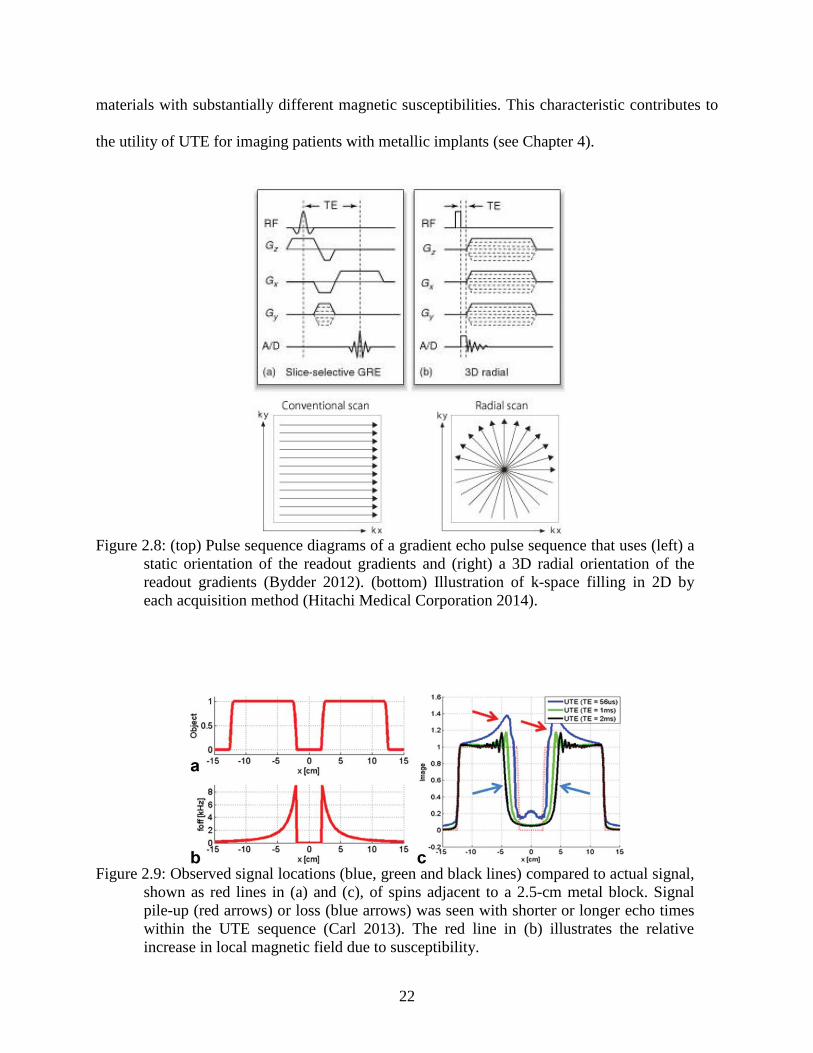
22
materials with substantially different magnetic susceptibilities. This characteristic contributes to
the utility of UTE for imaging patients with metallic implants (see Chapter 4).
Figure 2.8: (top) Pulse sequence diagrams of a gradient echo pulse sequence that uses (left) a
static orientation of the readout gradients and (right) a 3D radial orientation of the
readout gradients (Bydder 2012). (bottom) Illustration of k-space filling in 2D by
each acquisition method (Hitachi Medical Corporation 2014).
Figure 2.9: Observed signal locations (blue, green and black lines) compared to actual signal,
shown as red lines in (a) and (c), of spins adjacent to a 2.5-cm metal block. Signal
pile-up (red arrows) or loss (blue arrows) was seen with shorter or longer echo times
within the UTE sequence (Carl 2013). The red line in (b) illustrates the relative
increase in local magnetic field due to susceptibility.
23
CHAPTER 3: AIM 1, PHANTOM DEVELOPMENT
3.1 Overview
The goal of this aim was to develop a phantom that modeled human prostate tissue on a
3T MRI scanner. With implanted brachytherapy seeds, the phantom should produce images
suitable for assessing the appearance of brachytherapy seeds on UTE images.
As explained in Section 2.2.3, a T1 time constant of 1597 ms and a T2 time constant of
74 ms were the target values to model prostate tissue at 3T (Hattori 2013). To determine the
correct recipe, a series of twelve material compositions were tested; the T1 and T2 time constants
were evaluated for each. Of this series, four prostate phantom compositions closest to the target
T1 and T2 values were selected for the fabrication of a larger pelvic phantom to model a prostate
surrounded by non-prostate material in a region approximately the size of the adult male pelvis.
This chapter first describes the survey of material compositions, including the steps to
prepare the materials and the subsequent validation of the T1 and T2 values. Next, the
fabrication of the pelvic phantom is detailed. Finally, the process of seed implantation is
described including the acquisition of phase maps to assess B0 distortion by the titanium seeds.
3.2 Survey of Material Compositions
3.2.1 Target T1 and T2 time constants
The T1 and T2 time constants suggested by Hattori et al (2013) for prostate tissue were
T1=1597 ms and T2=74 ms. Other authors have reported a wide range of values for prostate
tissue T2 values. The average reported value for healthy prostate tissue in the central gland of the
prostate was a T2 time constant close to 80 ms, while cancerous tissue had a T2 time constant
anywhere from 82 ms to 110 ms (Foltz 2013, Weis 2013). For this thesis, both the T2 of healthy
prostate tissue and the longer T2 of cancerous prostate were modeled to test the limits of the
UTE technique. The T1 time constant of the phantom was more than an order of magnitude
24
larger than the T2 time constant, so T1 was expected to have little influence on the UTE
sequence.
3.2.2 Recipe and preparation of samples
Multiple material samples were created using variations of the recipe listed in Table 1
(Hattori 2013). These materials were dissolved in distilled water in the indicated quantities. The
amount of agarose adjusted T2 while the amount of GdCl3 altered T1. Of the remaining
components, carrageenan assisted with gelatinization, NaCl altered the conductivity of the
material, and NaN3 retarded the growth of molds or other microorganisms in the material. All
materials were purchased from Fisher Scientific (Fair Lawn, NJ), except carrageenan which was
purchased from Research Products International (Mt Prospect, IL).
Table 1: Concentrations to produce prostate-like T1 and T2 behavior on a 3T MRI (Hattori
2013).
Prostate tissue phantom material
composition
Suggested
concentration
by Hattori
Concentration
used in this
experiment
agarose 0.714% w/w 0.700% w/w
GdCl3 22.2 µmol/kg 22.2 µmol/kg
carrageenan 3% w/w 3% w/w
NaCl 0.291% w/w 0.200% w/w
NaN3 0.03% w/w 0.03% w/w
Figure 3.1 illustrates the preparation steps. The ingredients were measured, and then
dissolved in 97 mL of distilled water in a glass beaker to make 100 grams of prostate material.
The mixture was heated to 90°C for 5 minutes in a hot water bath while continuously stirred. To
prevent air bubbles from forming in the final phantom, the mixture was heated for an additional
20 minutes in the hot water bath without stirring. Each mixture was poured into a 7.5 cm

25
diameter plastic container and cooled to room temperature. The phantom material hardened upon
cooling and could then be removed from the container. A Foley catheter was inserted to model
the urethral opening in the center of the prostate phantom. The catheter was also used as a
marker for phantom orientation.
Figure 3.1: Steps of material preparation. Shown in the top row, (left) digital scale used to
measure chemicals, (center) mixing of chemicals, and (right) heating in a water bath.
Shown in the bottom row, (left) pouring mixture into a mold, (center) a solidified
prostate phantom, and (right) needle insertion into the prostate phantom.
3.2.3 T1 and T2 validation tests
To measure the T1 time constant, the inversion recovery technique was used (Hornak
2014). MRI images were acquired of the phantom for 6 inversion times (TI) with all other
parameters held constant. These parameters are listed in Table 2.
The images were loaded in MRmap (Messroghli 2012), a software program written in
IDL (Exelis Visual Information Solutions, Boulder, CO); a screenshot is shown in Figure 3.2. To
determine the T1 time constant, average signals were calculated for a region of interest placed

26
identically in the same slice of each inversion recovery image. The average signals were plotted
versus signal collection time and the T1 decay curve was fit to the data. As mentioned
previously, the T1 time constant was not expected to affect the UTE measurements, because T1
was at least an order of magnitude larger than T2.
Table 2: Parameters used to acquire inversion recovery images to measure the T1 relaxation
time of the phantom materials.
T1 time constant estimation protocol parameters
TE (echo time) 15.0 ms
TR (repetition time) 15 s
TI (inversion time) 1900,1600,1300,
800,600,500 ms
Echo train length
(number of 180°
rephasing pulses)
16
Receiver Bandwidth ± 31.25 kHz
Field of View 16.0 cm
slice thickness 5.0 mm
slice spacing 0.5 mm
Number of excitations 0.5
frequency encoding steps 256
phase encoding steps 256
frequency direction R/L
The T2 time constant was calculated with the multi-echo technique. In this technique, the
same slice was imaged 8 times during one TR with varying echo times. The parameters for these
scans are listed in Table 3. To measure the T2 time constant, an IDL-based software program
called H.A.N.D.-Dynamic MRI software tool (Hoffman 2012) was used. This program plotted
the signal intensity from each of the 8 images as a function of echo time for each pixel (Figure
3.3). An exponential decay curve of the net magnetization vector was fit to the graphed data
points and the T2 time constant for each pixel was determined. The resultant T2 time constant
values were averaged over a region of interest that was expected to be homogenous in the
phantom.

27
Figure 3.2: MRmap program used to estimate the T1 relaxation time of the phantom material
(Messroghli 2012).
Table 3: Parameters used to acquire spin echo images to measure the T2 relaxation time of
the phantom materials.
T2 time constant estimation protocol parameters
Number of echoes 8 echoes
TE (echo time)
7.26, 14.22, 21.34, 28.45,
35.56, 42.67, 49.78,
56.90 ms
TR (repetition time) 1650 ms
TI (inversion time) 50 ms
Receiver Bandwidth ±62.5 kHz
Flip angle 90 degrees
Field of View 14.0 cm
slice thickness 7.0 mm
slice spacing 4.6 mm
Number of excitations 1
frequency encoding steps 320
phase encoding steps 256
frequency direction R/L

28
Figure 3.3: Screenshot of the software program, H.A.N.D, used to measure the T2 relaxation
time of the phantom materials (Hoffman 2012). The first TE was not used for curve
fitting.
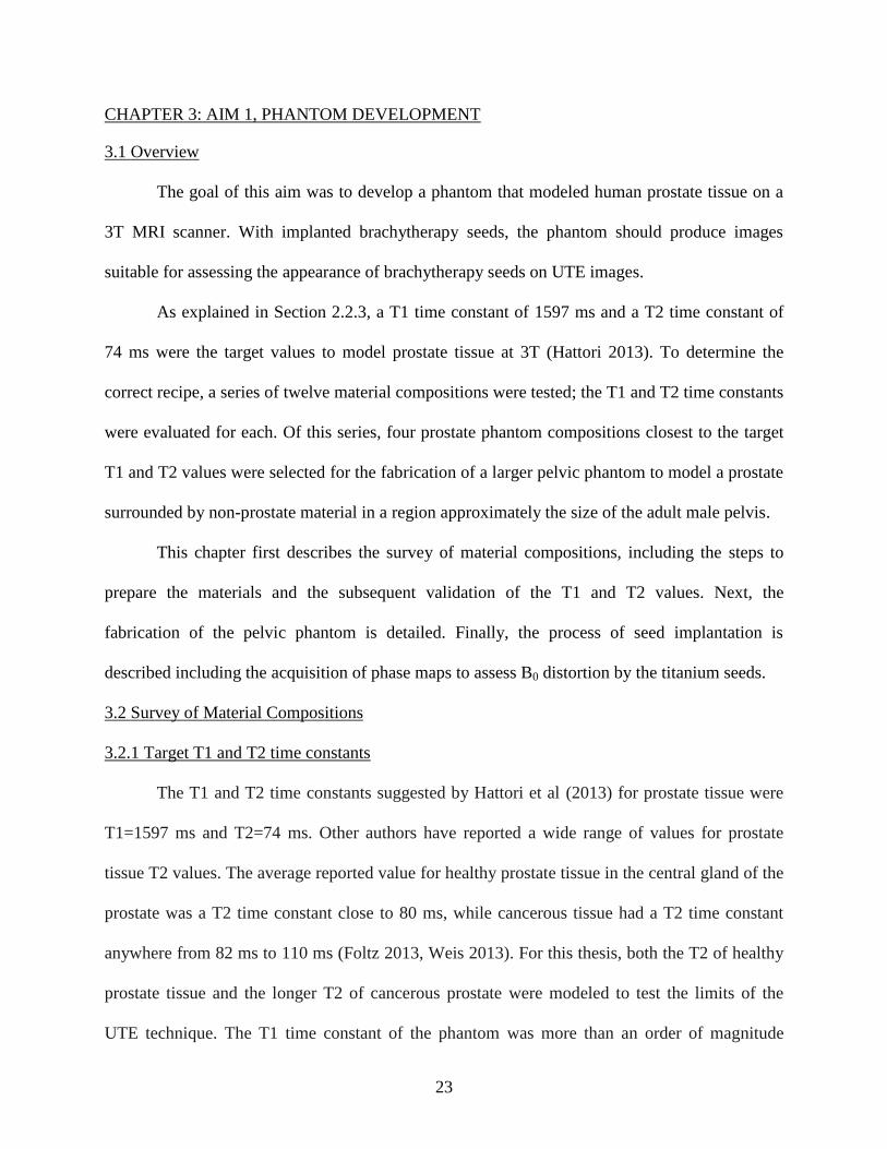
3.2.4 T1 and T2 validation results
The right column of Table 1 lists the recipe that resulted in T1 and T2 values closest to
the target values. T1-weighted and T2-weighted images for two representative materials are
shown in Figure 3.4. These two materials represented a cancerous prostate with shortened T1 and
lengthened T2 (Figure 3.4, left) and a healthy prostate with T1 and T2 close to the target values
(Figure 3.4, right). The “healthy” prostate tissue had T2 of 79 ms (target of 74 ms) while the
“cancerous” prostate had a T2 of 95 ms (target of 110 ms).
The measured T1 time constant for the “healthy” prostate was 1725 ms compared to the
target of 1597 ms. The “diseased” prostate had a shorter T1 than planned at 795 ms; this was due
to the difficulty of achieving a consistent T1 time constant. Small differences in the GdCl3
concentration occurred because of the small quantity required. Although not intended, this
material sample provided a means to see if a short T1 values would impact seed localization with
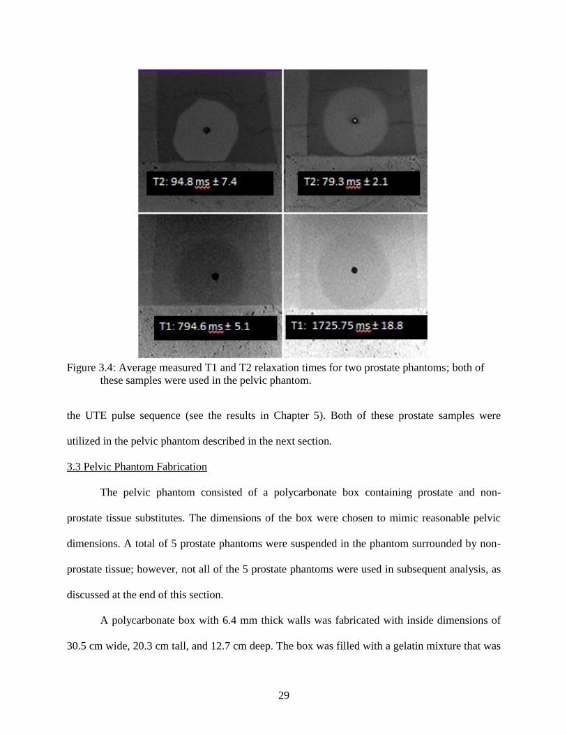
29
Figure 3.4: Average measured T1 and T2 relaxation times for two prostate phantoms; both of
these samples were used in the pelvic phantom.
the UTE pulse sequence (see the results in Chapter 5). Both of these prostate samples were
utilized in the pelvic phantom described in the next section.
3.3 Pelvic Phantom Fabrication
The pelvic phantom consisted of a polycarbonate box containing prostate and non-
prostate tissue substitutes. The dimensions of the box were chosen to mimic reasonable pelvic
dimensions. A total of 5 prostate phantoms were suspended in the phantom surrounded by non-
prostate tissue; however, not all of the 5 prostate phantoms were used in subsequent analysis, as
discussed at the end of this section.
A polycarbonate box with 6.4 mm thick walls was fabricated with inside dimensions of
30.5 cm wide, 20.3 cm tall, and 12.7 cm deep. The box was filled with a gelatin mixture that was

30
chosen to model the T1 and T2 values of muscle tissue. This material was mixed using
concentrations suggested by (Hattori 2013) using the same materials as the prostate, but with
altered concentrations to model T1 and T2 values of muscle (Table 4). This material was selected
to represent the worst case scenario because the time constants are similar to prostate, but
different enough for the two types of materials to be resolved on an MRI image. An initial layer
of 7-8 mm of muscle substitute was poured into the box and allowed to solidify (Figure 3.5).
Three prostate phantoms with values closest to the target T1 and T2 values were positioned
axially along the center of the box. Then, additional muscle mixture was filled around the
prostate phantoms so they remained suspended in the center of the field of view. The completed
pelvic phantom is shown in Figure 3.6. Once the pelvic phantom was hardened, the gelatin
material was solid enough to maintain its shape when removed from the polycarbonate box.
Table 4: Concentrations to produce muscle-like T1 and T2 behavior on a 3T MRI (Hattori
2013).
Muscle tissue phantom material composition
Suggested concentration
by Hattori
Concentration used in
this experiment
agarose 1.187% w/w 1.200% w/w
GdCl3 30.1 µmol/kg 55.0 µmol/kg
carrageenan 3% w/w 3% w/w
NaCl 0.291% w/w 0.291% w/w
NaN3 0.03% w/w 0.03% w/w
During fabrications, spray cans were inset into the muscle tissue to create voids where
other tissue substitutes could be added later if desired. Two additional prostate phantoms, pre-
implanted with physically pre-determined seed positions, were set into one void. However,
limitations in the available field of view of the UTE sequence precluded this portion of the
phantom from being used in subsequent analysis.

31
Figure 3.5: Creation of pelvic phantom. Three prostates were suspended in the center of the
pelvic phantom (only one is shown in this photo). The spray cans were used to create
voids for possible addition of other tissues.
Figure 3.6: Pelvic phantom after fabrication was complete but before seed implantation.
Additionally, a jar of petroleum jelly was set into the other void in the pelvic phantom to
assess possible heating of the titanium seeds by the UTE sequence. A seed was placed on the
surface of the petroleum jelly. Excessive heating of the seed would soften the jelly, causing the
seed to sink. The seed remained in its original location throughout the entire experiment
indicating no significant heating of the seed.

32
3.4 Seed Implantation
Three types of seeds were used in this study, which were all decayed to greater than 10
half-lives; these included: (1) STM-1251 iodine-125 radioactive sources (BARD Medical, Inc),
(2) AgX-100 iodine-125 (Theragenics), and (3) palladium-103 sources (Theragenics). The
specifications of the STM-1251 I-125 source are shown in Figure 3.7 (Rivard 2004); a photo of a
seed was shown in Figure 1.2.
Figure 3.7: Specifications for the BARD brachytherapy seed used to model seed implantation
in this project (Rivard 2004).
After removing the solidified pelvic phantom from the box, the brachytherapy seeds were
implanted in the prostate phantoms located in the center of the pelvic phantom. The seeds were
implanted using both standard spacing and random spacing as shown in Figure 3.8 and Figure
3.9. The seeds were implanted so they would be oriented parallel to B0 when scanned in Aim 2.
As discussed in section 1.3, every brachytherapy treatment is tailored to the patient’s prostate
size and shape; in a typical implant, seeds can be more concentrated in some areas and less in
others. The most common method of seed implantation consists of each seed connected with a 5
mm spacer (Figure 3.9). Alternatively, seeds can be linked with 0.5 mm spacing. Both spacing
arrangements were modeled in the pelvic phantom. Finally, single seeds were placed to represent
deviations from intended placement, for use in Aim 3.

33
Figure 3.8: Steps for seed implantation. The seed strands before implantation and the needle
used for seed implantation.
Figure 3.9: SourceLink spacers used to space the seeds in different configurations. The seed
spacers were made of 70:30 poly(L-lacgtide-co-D,L-lactide). (BARD Medical)
3.4.1 Phase maps to assess B0 distortion by titanium seeds
As a supplemental test for the proof of concept, a phase map was collected to map the
phase differences throughout the pelvic phantom. As mentioned in section 2.5, each pixel in the
phase map represents the magnitude of the difference in precessional frequency compared to the
Larmor frequency.

34
Figure 3.10 (left) is a typical gradient-recalled echo image of the pelvic phantom with 10
seeds plus the urethra. Figure 3.10 (right) is the phase difference map of the same slice, which
represents the difference between B and B0. The large ring-shaped patterns at the right and left
sides of the image are phase wrapping artifacts, which were explained in section 2.5. The phase
difference increased dramatically in the vicinity of the seeds, due to magnetic susceptibility
causing changes in local field strength. This large gradient contributes to chemical shift artifacts,
which are described in Chapter 4 as a method to identify seeds.
Figure 3.10: A gradient echo based image (left) and the corresponding phase difference map
(right) of the pelvic phantom after the seeds were implanted.
The phase maps revealed that the B0 is substantially distorted close to the seed’s edge, a
key aspect to the expected utility of the UTE sequence. In the phase map, seed locations could be
identified, but metal did not appear different from other artifacts like air bubbles. This result
indicated that phase maps themselves cannot be used to differentiate metal seeds from other non-
metal artifacts.

35
3.5 Discussion
After the seeds were implanted with the same needles used by physicians in a typical
procedure, the gelatin was hardened enough not to reform around the needle tracks. This could
have also contributed to errors with the introduction of air to the phantom material causing
altered seed visualization. Seed trains over the entire length prostate phantom were used to
minimize this error.
3.5.1 Seed placement
The needles used to implant the brachytherapy seeds into the pelvic phantom were
created to slightly bend when implanted into the prostate to enable the physician to counteract
the swelling or resistance in the patient anatomy. As a result, the seeds were not implanted
exactly in alignment with B0. This is common for clinical procedures as well, but when
combined with an inexperienced “surgeon”, many seeds were implanted closer together than
intended. This could lead to miscounts even with the gold standard counting method, CT
(Lindsay 2003). In reality, the seeds would not be implanted in such a manner, so this
represented the worst possible case scenario that modeled an unskilled implantation procedure.
To remediate this error, a possible solution would be to have an experienced surgeon implant the
seeds into the phantom, or use patient data that represents clinically acceptable seed spacing.

36
CHAPTER 4: AIM 2, IMAGE ACQUISITION AND QUALITY ASSESSMENT
4.1 Overview
The goal of this aim was to acquire UTE MRI images to assess the utility of UTE for
post-implant dosimetry. The quality of the images was assessed through qualitative and
quantitative metrics. The final scan parameters were selected to help create post-implant
dosimetry guidelines in Aim 3.
4.2 Materials and Methods
Using the pelvic phantom described in the previous chapter, MRI scans were collected to
determine which pulse sequence parameters affect the quality of images to be used for post-
implant dosimetry. The scanner used in this procedure was a 3T GE Signa HDxt MRI scanner
with version 16.0 software located at Pennington Biomedical Research Center. The phantom was
scanned with multiple parameter combinations that were compared qualitatively for best seed
visualization. Then, the image quality was assessed using the following parameters: signal-to-
noise ratio (SNR), contrast-to-noise ratio (CNR), signal contrast between seed and prostate
tissue, and apparent seed diameter (with line profile).
4.2.1 Phantom setup
The phantom was oriented on the MRI scanner to match a typical prostate patient setup
as closely as possible (Figure 4.1). An 8-channel torso array coil was used. The prostate phantom
was centered in the field of view roughly 125 cm above the table.
4.2.2 UTE acquisition parameters
The 3D UTE pulse sequence used in this study was provided by Dr. Jiang Du from the
Department of Radiology at the University of California, San Diego. The pulse sequence and
reconstruction programs were loaded onto the PBRC MRI workstation. Program configuration

37
was edited to match the program code to be compatible with the software version of the PBRC
workstation. The UTE scan parameters are listed in Table 5.
Figure 4.1: Illustration of the phantom setup in the MRI scanner.
Table 5: MRI parameters used to collect a UTE image of the pelvic phantom. (Personal
communication with J. Du, UCSD, 2013).
UTE parameters
TR 12 ms
TE 30 µs or 60 µs
Receiver Bandwidth ± 31.25 Hz, ± 62.5 Hz,
or ± 125 Hz
Flip angle 9 degrees, 14 degrees,
or 30 degrees
Field of View (FOV) 18.0 cm x 18.0 cm
Slice thickness 0.7013 mm
Slice spacing 0.7813 mm (isotropic 3D
resolution)
Frequency encoding steps 256
Phase encoding steps 256
Imaging plane Axial
Number of radial k-space
projections 40,000

38
4.2.3 Fast Spin Echo acquisition parameters
Image data was also acquired with a fast-spin echo (FSE) pulse sequence. FSE was used
for comparison because this is the most commonly used T2-weighted imaging sequence to
provide adequate prostate soft tissue contrast (Bowes 2013). The FSE parameters are
summarized in Table 6.
Parameters were chosen to match the typical clinical parameters for post-implant
dosimetry. Only the FOV was specifically matched to the UTE parameters; other UTE scan
parameters do not have an obvious parallels with FSE parameters. For example, the UTE
sequence is 3D, while the typical FSE scan used for comparison was 2D. In particular, TE and
TR were substantially different between UTE and FSE due to the unique nature of the UTE
sequence.
Additionally, the bandwidth was different between the scans. The 3D nature of the UTE
sequence required a shorter selection of bandwidth, while literature review of typical T2-
weighted FSE scan parameters intended for post-implant dosimetry imaging suggested a higher
bandwidth. For comparison, the “best case scenario” for each imaging sequence was selected.
These best cases highlight the positive features and advantages of each pulse sequence.
Table 6: Recommended pulse sequence parameters to collect a T2-weighted image at 3T
used for post-implant dosimetry (Bowes 2013).
Fast spin echo parameters
TE 90 ms
TR 3775 ms
ETL 10
Receiver BW ± 20.8 kHz
FOV 20.0 cm
slice thickness 3 mm
slice spacing 3 mm
frequency encoding steps 320
phase encoding steps 224
Frequency direction R/L

39
4.3 Results and Discussion
4.3.1 Signal pile-up phenomenon
Signal pile-up is a phenomenon that occurs when a tissue is imaged in proximity to a
material with a large magnetic susceptibility, such as prostate tissue with implanted titanium
brachytherapy seeds. As reviewed in section 2.3, applied gradients allow the data to be spatially
sorted depending on the frequency of the net magnetization vector in each voxel. The magnetic
susceptibility of adjacent materials changes the local B-field strength causing spins to precess at
a rate different than the Larmor frequency. These spins are misplaced at a spatial position that is
not the true physical location of the spins (Figure 4.2). Signal pile-up describes the magnitude of
displaced signals registered to a specific voxel, causing a signal intensity difference from voxels
that are more distant from the high-susceptibility material (Carl 2013).
(4.1)
Equation 4.1 describes the relationship between the distance of the spatial shift (Δx), the
field of view in the readout direction (FOVx), the shift in frequency (Δω), and the full bandwidth
(e.g. rBW of ± 16 kHz = full BW of 32 kHz).
Figure 4.2: Illustration of the signal pile-up effect where signal is shifted spatially to a falsely
represented location in the spatial position image (Bydder 2012).

40
This effect is illustrated in Figure 4.3 for image data acquired in this project, where
sagittal views of 3 seeds from two UTE image acquisitions are shown. The FOV of the first trial
(Figure 4.3, left) was 2 cm larger than the second trial (Figure 4.3, right), with bandwidth and
other parameters held constant. The appearance of the pile-up effect was completely inverted, as
illustrated in the cartoons below the UTE images. This showed that the relationship between
FOV and Δx strongly impacts the appearance of the seeds, which could result in
misinterpretation of seed locations.
Figure 4.3: Sagittal view of 3 seeds from two trials of UTE acquisition, with (top) 20 cm
FOV compared to (bottom) 18 cm FOV. The cartoons illustrate where the pile up
occurred relative to the centers of the seeds.
4.3.2 Apparent seed size
One parameter used to quantify the pile-up effect was apparent seed diameter, which was
essentially the diameter of the pile-up artifact. As discussed previously, a brachytherapy seed
itself does not provide signal on a proton-based MRI scan, due to the lack of hydrogen in the
titanium implant. However, the pile-up effect shifted tissue signals immediately adjacent to the
titanium seeds, which was visualized with UTE. The signal pile-up from the protons immediately
adjacent to the seeds resulted in positively contrasted, or bright, borders for the seeds. This
susceptibility artifact occurs in all MRI images with metallic implants, but the visualization of
the artifact is usually lost with the conventional use of relatively long TE; seeds show up as black

41
voids indicative only of a lack of spins because the susceptibility artifact de-phases too quickly
before the signal can be acquired. UTE captures the pile-up signal before it can be lost.
The apparent seed diameter was used to quantify the amount of pile-up effect. Seed
diameter was determined as the full width at half maximum of the seed in a line profile,
comparing the peak in the line profile to the average noise level. The line profile across a seed
was measured with the line profile tool in ImageJ (Rasband 1997-2014). The line profiles are
shown in Figure 4.4 for one seed in UTE and FSE images of an implanted prostate phantom.
Figure 4.5 plots the line profiles on the same graph to emphasize the greatly increased signal
magnitude in the UTE image due to the susceptibility artifact.
Based on 80 seed measurements, the average apparent seed diameter measured on the T2
weighted FSE image was 1.46 ± 0.38 mm. The apparent seed diameter increased with increasing
bandwidth on the FSE image. For the same 80 seeds measured on the UTE images, the average
apparent seed diameter was 4.65 ± 0.63 mm. The exaggerated seed diameter made the seeds
more visually apparent. This could lead to improvement of seed counting accuracy which will be
discussed in Aim 3.
Figure 4.4: Line profile measurements measured in ImageJ (Rasband 1997) for the same slice
in both UTE and FSE images. The line profiles plot pixel intensity along the blue line
in each image.
UTE FSE

42
Figure 4.5: Line profiles for the same seed from both FSE and UTE displayed on the same
scale. This graph illustrates the ability of UTE to capture the large signal magnitude
due to pile-up.
4.4 Discussion of UTE Parameter Variations
4.4.1 Receiver bandwidth
Changes in receiver bandwidth altered apparent seed size. The pile-up intensity appeared
to increase with lower bandwidth. As seen in Figure 4.6, for the same slice as well as the same
window and level adjustments, when the bandwidth was varied, the seeds appeared larger and
brighter for the lower bandwidth. This was a result of the relationship between shift size and

43
bandwidth for individual frequency offsets (Equation 4.1). The relationship between SNR and
receiver bandwidth is:
√
(4.2)
which illustrates how a larger bandwidth resulted in a decrease in the pile-up effect for the same
slice in a UTE image.
Figure 4.6: Three different receiver bandwidths used to acquire the same image slice with
UTE. Note how the appearance of the bright ring (pile-up artifact) around a seed
decreases with increasing bandwidth.
The lowest bandwidth was selected at ± 31.25 kHz because another relationship that
affects the image quality is the relationship between TE and rBW. TE increases as rBW
decreases. Too small of an rBW (a shallow linear gradient) causes the TE to increase (to fit the
whole gradient) to too high of a value, reducing the ability of UTE to capture the magnetic
susceptibility artifact.
4.4.2 Flip angle
Another user-defined parameter that affected image quality was flip angle. A smaller flip
angle (the amount that M0 is perturbed from the z-axis) forces a shorter signal collection time,
but a large flip angle reduces the ability to see pile-up effects because the susceptibility-induced

44
T2 shortening results in signal decay prior to signal acquisition (after the RF pulse is completed).
Variations in the flip angle showed that the signal pile-up effect was most intense visually for a
flip angle of 15 degrees (Figure 4.7). This relationship can be explained by the Ernst angle.
Figure 4.7: Three different flip angles used to acquire the same image slice with UTE.
The Ernst angle relationship is the flip angle for a spin that give the maximum signal
intensity in the shortest amount of time (Haacke 1999). This flip angle is dependent on the TR
and T1 relaxation time of the imaged tissue. The Ernst angle (αE) is given by:
( ) (4.3)
and illustrated in Figure 4.8. For the “healthy” and “diseased” prostate phantoms imaged in this
experiment, the Ernst angles were 7° and 10°. An interesting observation was that the images
acquired at 15° appear to display more contrast between the prostate material and the pile-up
artifact surrounding the seeds, although this results from the decrease in prostate signal with flip
angle rather than a change in pile-up artifact.
Because the seed presented as a bright signal, the higher contrast between seed and
prostate occurred when the prostate material was not at its maximum value. Therefore, using a
flip angle just above the Ernst angle caused the seed to appear with more contrast. Unfortunately,

45
Figure 4.8: Relative transverse signal intensity as a function of flip angle. The Ernst angle is
flip angle where the signal intensity is highest.
too large of a flip angle leads to a long TR, causing acquisition time to be too long for a
convenient patient scan time. Therefore a flip angle of 15 degrees was selected.
4.5 UTE and FSE Comparison
UTE and T2-weighted FSE images were compared. Various parameters were selected for
quantitative comparison including signal-to-noise ratio (SNR) and contrast-to-noise ratio (CNR).
Additionally, qualitative parameters were examined including seed visibility and artifacts.
4.5.1 Regions of interest
To measure SNR and CNR between various sections on the UTE images, a region of
interest was drawn on each slice. A sample of a few of the hundreds of regions of interest drawn
to collect the data are shown in Figure 4.9.
4.5.2 SNR
The SNR was compared for the UTE and FSE images with the same bandwidth (Table
7). The SNR was measured with regions of interest within the prostate phantom adjacent to the
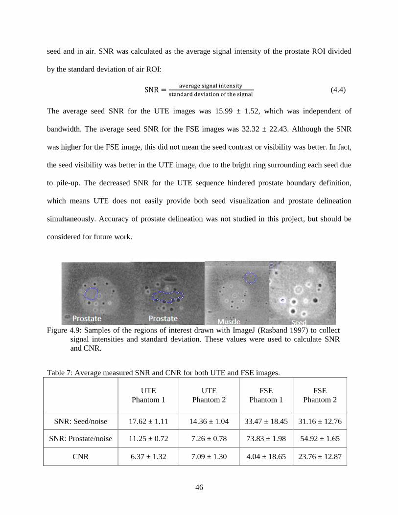
46
seed and in air. SNR was calculated as the average signal intensity of the prostate ROI divided
by the standard deviation of air ROI:
(4.4)
The average seed SNR for the UTE images was 15.99 ± 1.52, which was independent of
bandwidth. The average seed SNR for the FSE images was 32.32 ± 22.43. Although the SNR
was higher for the FSE image, this did not mean the seed contrast or visibility was better. In fact,
the seed visibility was better in the UTE image, due to the bright ring surrounding each seed due
to pile-up. The decreased SNR for the UTE sequence hindered prostate boundary definition,
which means UTE does not easily provide both seed visualization and prostate delineation
simultaneously. Accuracy of prostate delineation was not studied in this project, but should be
considered for future work.
Figure 4.9: Samples of the regions of interest drawn with ImageJ (Rasband 1997) to collect
signal intensities and standard deviation. These values were used to calculate SNR
and CNR.
Table 7: Average measured SNR and CNR for both UTE and FSE images.
UTE
Phantom 1
UTE
Phantom 2
FSE
Phantom 1
FSE
Phantom 2
SNR: Seed/noise 17.62 ± 1.11 14.36 ± 1.04 33.47 ± 18.45 31.16 ± 12.76
SNR: Prostate/noise 11.25 ± 0.72 7.26 ± 0.78 73.83 ± 1.98 54.92 ± 1.65
CNR 6.37 ± 1.32 7.09 ± 1.30 4.04 ± 18.65 23.76 ± 12.87

47
4.5.3 CNR
The CNR was calculated for both UTE and FSE images. The CNR was measured with a
ROI surrounding the seed, an ROI in the prostate tissue phantom near the seed, and an ROI in
air. CNR was calculated as the ratio of the difference between the average prostate signal
intensity and the average seed signal intensity to the standard deviation of those measurement
regions:
( ) ( ) (4.5)
Listed in Table 7, the average CNR for the UTE images with ± 31.25 kHz bandwidth was 6.73 ±
1.85. The average CNR for the FSE images was 23.76 ± 12.87. Although the CNR was larger for
the FSE image, seeds cannot be distinguished from air because both present as signal voids.
4.5.4 Qualitative assessment
Qualitatively, overall seed visibility appeared to be better with UTE. This was attributed
to the bright ring-shaped pile-up artifact around the seed. At very short echo times, the positive
contrast visualization of the seeds was clearly distinct from the appearance of other artifacts (e.g.
air cavities) due to the different magnitudes of magnetic susceptibility. The phase difference
maps in Figure 4.10 showed that the highest change in susceptibility in fact appeared near air
bubbles. However, air bubbles should not be present within the prostate in vivo and in any case
would be unlikely to have the same size as seeds.
The slice montage in Figure 4.11 shows the formation of a seed signal as compared to the
formation of an air bubble signal (Figure 4.12). The arrows show the bright center of the seed in
between slices with a bright ring. Also, the arrows show an air bubble that is similar in size to a
seed; the air bubble lacks the bright center, indicating an artifact rather than a seed.
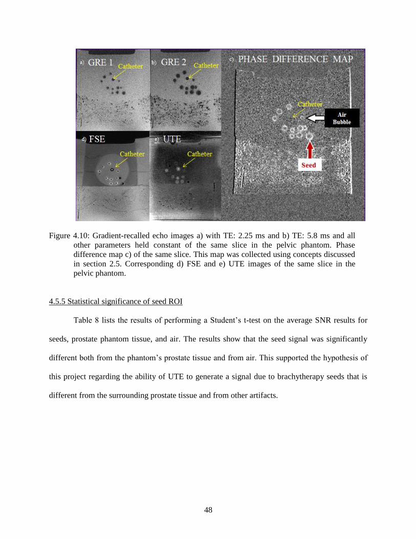
48
Figure 4.10: Gradient-recalled echo images a) with TE: 2.25 ms and b) TE: 5.8 ms and all
other parameters held constant of the same slice in the pelvic phantom. Phase
difference map c) of the same slice. This map was collected using concepts discussed
in section 2.5. Corresponding d) FSE and e) UTE images of the same slice in the
pelvic phantom.
4.5.5 Statistical significance of seed ROI
Table 8 lists the results of performing a Student’s t-test on the average SNR results for
seeds, prostate phantom tissue, and air. The results show that the seed signal was significantly
different both from the phantom’s prostate tissue and from air. This supported the hypothesis of
this project regarding the ability of UTE to generate a signal due to brachytherapy seeds that is
different from the surrounding prostate tissue and from other artifacts.

49
Figure 4.11: A seed (white arrow) on 8 consecutive slices (0.7013 mm thick). The red arrow
shows where the pile-up in the center of the ring that is used to identify the presence
of a seed on the UTE image.
Figure 4.12: An air bubble (white arrow) on 4 consecutive slices (0.7013 mm thick). This
shows the lack of bright center that the seed characteristically displays on the same
scan.
Table 8: Results from Student’s t-test performed on the average SNR results for seed prostate
and air signal.
Hypothesis Corresponding p values
Seed signal> prostate signal p<0.05
Seed signal > air signal p<0.001

50
CHAPTER 5: AIM 3, SEED LOCALIZATION PROCEDURE AND RECONSTRUCTION
ACCURACY
5.1 Overview
The goal of this aim was to develop guidelines for brachytherapy seed counting with the
UTE MRI pulse sequence. Instructions were drafted that described how to identify seeds based
on the observations of seed appearance (artifacts) reported in Chapter 4. Two experienced
physicists counted the seeds on the same set of phantom images. The purpose of this aim was to
establish a baseline method that could be subsequently refined for investigation with patient data.
5.2 Materials and Methods
The images collected from Aim 2 were used to develop criteria for identifying seeds. In
the future, an automatic seed localization program may be conceivable, but such development
was outside the scope of this project.
5.2.1 Seed configuration
The pelvis phantom was implanted with 18 strands of titanium seeds that mimicked
common seed distributions in patient plans. The seeds were connected using BARD spacers as
shown in Figure 3.9; one configuration consisted of seeds spaced equally apart, shown in the
lower part of Figure 5.1. A variety of configurations was implanted to test the capabilities of
UTE imaging to identify seeds in different geometries.
5.2.2 Characteristics of seed appearance on UTE images
The center of a seed appeared as a bright white spot. On the superior and inferior axial
slices, a seed appeared to have a central black spot bordered with a thick white ring. Figure 5.2,
Figure 5.3 and Figure 5.4 show an illustration prepared to train observers in the appearance of
seeds and other structures in a UTE image.

51
Figure 5.1: Seed configurations implanted. The varied configuration (top) was used to test
the seed localization accuracy and the standard configuration (bottom) was used for
reference.
Figure 5.2: Comparative orthogonal views of the same location on both UTE and FSE
images. The spacing between the beginning of two seed strands (1) is almost double
the spacing towards the end of the same two seed strands (2) as highlighted in the
Coronal UTE image
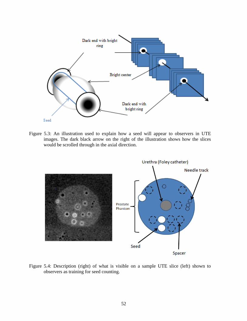
52
Figure 5.3: An illustration used to explain how a seed will appear to observers in UTE
images. The dark black arrow on the right of the illustration shows how the slices
would be scrolled through in the axial direction.
Figure 5.4: Description (right) of what is visible on a sample UTE slice (left) shown to
observers as training for seed counting.

53
5.2.3 Seed counting guidelines
Two physicists experienced in post-implant dosimetry for prostate brachytherapy
volunteered to participate in this experiment. The physicists were given directions for seed
identification on ImageJ (Rasband 1997-2014). The instructions were:
A seed will always have a bright ring before and after the bright white center. If you
see a ring not followed by a bright white center, it is an artifact. Some seeds have a
tiny white dot in the center which indicates the center of the seed. Not all seeds have
this. Some are simply a solid white spot. Both are considered a seed to be counted.
When two seeds are implanted without a spacer between them, the signal pile-up
effect is compromised, and appears slightly different than if there was a spacer
between the two.
Step 1: Locate the seed in the axial view using the yellow cursor (cf. Figure 5.5).
Step 2: Confirm the seed is positioned within a strand using the corresponding
orthogonal views (cf. Figure 5.6).
Representative images that accompanied the instructions are shown in Figure 5.5 (for Step 1) and
Figure 5.6 (for Step 2).
Figure 5.5: Axial view of seed on UTE image. The yellow cursor is centered on the seed by
the observer.
Figure 5.6: The corresponding coronal (left) and sagittal (right) views of the seed centered in
Figure 5.5.

54
5.3 Results and Discussion
5.3.1 Exclusion of slices at edge of FOV
When the final UTE scans were collected, an unanticipated artifact was seen in the slices
adjacent to the polycarbonate walls of the pelvis phantom (Figure 5.7). Slices near the box walls
exhibited an elevated intensity, strongest adjacent to the box walls and decreasing with distance
from the wall. This elevated intensity masked the appearance of the main attribute of the seeds in
the UTE sequence. Bright pixel values indicate shortened T2 in this region. However, it was
uncertain if the artifact was caused directly by the polycarbonate material (i.e. the polycarbonate
influenced the apparent T2 of the phantom material), if polycarbonate has an ultra-short T2
component of its own, or if the phantom material solidified in a structured manner due to
proximity to the polycarbonate that caused a reduction in T2. Regardless of the cause, the 10
slices adjacent to each polycarbonate wall, where this artifact was apparent, were excluded from
the slices used to test the feasibility with physicists counting the seeds.
Figure 5.7: Area of elevated signal intensity due to the contamination of ultra-short T2 signal
from the polycarbonate walls of the pelvic phantom. The outlined areas (labeled
“Area of Failure”) were excluded in the localization tests
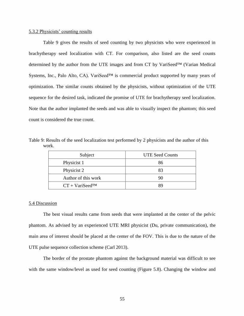
55
5.3.2 Physicists’ counting results
Table 9 gives the results of seed counting by two physicists who were experienced in
brachytherapy seed localization with CT. For comparison, also listed are the seed counts
determined by the author from the UTE images and from CT by VariSeed™ (Varian Medical
Systems, Inc., Palo Alto, CA). VariSeed™ is commercial product supported by many years of
optimization. The similar counts obtained by the physicists, without optimization of the UTE
sequence for the desired task, indicated the promise of UTE for brachytherapy seed localization.
Note that the author implanted the seeds and was able to visually inspect the phantom; this seed
count is considered the true count.
Table 9: Results of the seed localization test performed by 2 physicists and the author of this
work.
Subject UTE Seed Counts
Physicist 1 86
Physicist 2 83
Author of this work 90
CT + VariSeed™ 89
5.4 Discussion
The best visual results came from seeds that were implanted at the center of the pelvic
phantom. As advised by an experienced UTE MRI physicist (Du, private communication), the
main area of interest should be placed at the center of the FOV. This is due to the nature of the
UTE pulse sequence collection scheme (Carl 2013).
The border of the prostate phantom against the background material was difficult to see
with the same window/level as used for seed counting (Figure 5.8). Changing the window and

56
level helped to visualize the prostate border, although the border was always better evident in
FSE images.
Figure 5.8: A selected slice with poor prostate definition on the UTE image (left) and slightly
improved prostate definition on the corresponding FSE image (right).
The seed counts exceeded 92% accuracy for all users, compared to reported seed
localization accuracies of about 70% with other post-implant MR sequences (Bowes 2013). This
method did not achieve the 100% accuracy desired from post-implant dosimetry imaging (Bowes
et al. 2013), but as noted previously, the UTE parameters used here were selected as best guesses
and were likely not optimal. One observation was the background signal’s interference with the
seed signal appearance in areas with a high signal present from the prostate phantom with a short
T1 relaxation time (795 ms compared to the accepted 1600 ms for prostate tissue). This short T1
was not wholly representative of prostate tissue, but the observation was interesting because it
indicated that seeds present in a tissue with a short T1 relaxation time would be more difficult to
visualize; combined with the small FOV necessary for acceptable patient imaging times, this
may have implications for detecting seeds that have migrated out of the prostate.

57
An addition to the procedure, suggested by one physicist, was to use the orthogonal views
to help confirm seeds versus artifacts. It proved advantageous to use an orthogonal view of the
seeds because the distinct pattern of the seeds in the sagittal plane helped clarify the reader’s
uncertainty. Orthogonal views are not typically used with other methods for seed counting
(fusion or CT) due to thicker slices with poor seed definition in the axial direction.
The use of the 3D UTE sequence could be a significant factor to improve the accuracy of
seed localization on MRI. A 3D scans provides isotropic resolution with good seed definition in
all directions, while the distinctive pile-up effect can be captured with UTE.
5.4.1 Patient scans of UTE without seeds
In Figure 5.9, a healthy patient was scanned with the UTE protocol parameters acquired
with 5° and 20° flip angles from Table 5. Both images in Figure 5.9 used the same echo time (30
µs). The smaller flip angle resulted in a noiser image; both images showed the presence of bright
short-T2 areas surrounding the prostate that could potentially interfere with seed localization.
Further UTE studies of patients with implanted seeds are required to investigate how realistic
patient anatomy will affect seed localization accuracy with UTE.

58
Figure 5.9: UTE scans of the prostate of a healthy volunteer. The top image shows contours
of the prostate, bladder and rectum for the same patient in the bottom images.

59
CHAPTER 6: CONCLUSION
6.1 Summary of results
This study demonstrated that UTE is a feasible alternative for localizing titanium prostate
brachytherapy seeds after implantation, specifically BARD STM-6711 iodine-125 seeds. Results
indicated that UTE-based post-implant images were sufficient to differentiate seeds from
artifacts caused by the presence of air bubbles (p<0.05) and prostate (p<0.001). The ability to
accurately identify seed from non-seed material is critical for MR-based post-implant dosimetric
calculations. Prostate delineation quality for UTE images was decreased compared to FSE.
Overall, UTE imaging yielded image sets with apparently sufficient differentiation to facilitate
seed localization for post-implant permanent brachytherapy seed dose calculations in the
prostate.
6.2 Response to hypothesis
UTE was capable of differentiating titanium seeds from prostate and air bubble artifacts,
evidenced by the statistically significant increased signal from the titanium seeds on UTE when
compared to the signal from both prostate (p<0.001) and air (p<0.05). The results of this project
led to the conclusion that the UTE pulse sequence is better than T2-weighted FSE MRI for seed
identification because it distinctively visualized metallic seeds from air bubbles and prostate
tissue. However, the UTE pulse sequence was worse than FSE in terms of SNR, which led to an
ambiguous prostate outline on the UTE image. Additionally, the apparent diameter of the seeds
localized on the UTE scan was much larger than the true diameter; while helpful for qualitative
visualization, how this might quantitatively impact dosimetric results was not studied.
6.3 Recommendation
This study clearly demonstrated the potential utility of UTE for visualization of
brachytherapy seeds, using acquisition parameters identified from the literature on UTE in other

60
applications. An optimum imaging protocol should be developed through a more complete
survey of UTE parameter space. At this time, we recommend that the UTE pulse sequence be
used for manual seed identification, in conjunction with T2-weighted MRI for prostate
delineation. The UTE pulse sequence is not recommended as a stand-alone imaging technique; in
particular, UTE requires a relatively small field of view, which may limit its utility for situations
where seeds have migrated out of the prostate. As mentioned, a complete survey of parameter
space, including aspects of bandwidth and field of view, would be a valuable extension of this
work.
6.4 Limitations of the study
This feasibility study used UTE acquisition parameters that were based on application of
UTE to situations other than the prostate, with a limited investigation of overall parameter space.
As such, these parameters were likely not optimal for visualization of seeds with appropriate
field of view, bandwidth, imaging time, etc. This study only modeled two variations of prostate
tissue (with different T1 and T2 relaxation constants) in a homogeneous phantom, and did not
include a variety of complications that may be encountered in vivo, e.g. calcifications and blood
clots. These confounding factors could impact a UTE-based localization technique. While one
could conceive of further phantom-based studies that include additional relaxation constants,
more complex anatomy, or other complicating facets; moving to an in vivo study seems most
appropriate for future studies.
6.5 Future work
As mentioned previously, a thorough survey of parameter space is recommended for
protocol optimization. This survey should likely be a combination of phantom and in-vivo

61
imaging assessment. Of particular interest will be the parameters that directly affect seed
appearance (for instance, receiver bandwidth) and SNR or CNR.
Spatial distortions for the UTE sequence should also be characterized. As noted, some
seed trains appeared curved in the UTE images. Some needle deflection was likely caused by the
flexibility of the implantation needle and the relatively stiff phantom material. Although the
pelvis phantom was fabricated with alignment marks on the box, the limited field of view in the
feasibility study was too small to include the marks, thus precluding an assessment of spatial
non-uniformity in UTE scans.
Another area of possible investigation is task-based assessment of seed localization and
its impact on dosimetric accuracy. This would require UTE images of many prostate seed
implants; multiple readers would determine seed locations and orientations. Accuracy could be
assessed with the localization data itself or with post-implant plans calculated from the
localization data. Along with this, the distinctive pattern of the seeds in the UTE images suggests
the possibility of developing an automated localization algorithm.
Finally, the literature reports that a number of pulse sequences are being investigated for
prostate imaging, such as diffusion-weighted imaging or contrast-enhanced MRI (Tanaka 2006,
Katayama 2011, Bowes 2013). However, these protocols focus on imaging of the prostate for
diagnosis. The ability (or lack thereof) of these pulse sequences to visualize brachytherapy seeds
should be investigated and compared to UTE.

62
REFERENCES
Bowes, D., Crook, J. M., Araujo, C., Batchelar, D. (2013). "Ultrasound-CT fusion compared
with MR-CT fusion for postimplant dosimetry in permanent prostate brachytherapy."
Brachytherapy 12(1): 38-43.
Bowes, D., Crook, J. M., Rajapakshe, R., Araujo, C., Parker, B. (2013). "Defining a magnetic
resonance scan sequence for permanent seed prostate brachytherapy postimplant
assessment." Brachytherapy 12(1): 25-29.
Brown, A. P., Pugh, T. J., Swanson, D. A., Kudchadker, R. J., Bruno, T. L., Christensen, E. N.,
van Vulpen, M., Frank, S. J. (2013). "Improving prostate brachytherapy quality assurance
with MRI-CT fusion-based sector analysis in a phase II prospective trial of men with
intermediate-risk prostate cancer." Brachytherapy 12(5): 401-407.
Bydder, G. M., Fullerton, G. D., Young, I. R. (2012). MRI of Tissues with Short T2s or T2*s.
Chichester, West Sussex, UK, John Wiley & Sons, Ltd.
Carl, M., Koch, K., Du, J. (2013). "MR imaging near metal with undersampled 3D radial UTE-
MAVRIC sequences." Magn Reson Med 69(1): 27-36.
CDC (2013). "Prostate Cancer" Cancer Prevention and Control, Centers for Disease Control and
Prevention.
Crook, J. M., Patil, N., Ma, C., McLean, M., Borg, J. (2010). "Magnetic resonance imaging-
defined treatment margins in iodine-125 prostate brachytherapy." Int J Radiat Oncol Biol
Phys 77(4): 1079-1084.
Davis, B. (2012). "American Brachytherapy Society Consensus Guidelines for Transrectal
Ultrasound-guided Permanent Prostate Brachytherapy." Brachytherapy 11(1): 6-19.
De Brabandere, M., Hoskin, P., Haustermans, K., Van den Heuvel, F., Siebert, F. A. (2012).
"Prostate post-implant dosimetry: interobserver variability in seed localisation,
contouring and fusion." Radiother Oncol 104(2): 192-198.
De Brabandere, M., Kirisits, C., Peeters, R., Haustermans, K., Van den Heuvel, F. (2006).
"Accuracy of seed reconstruction in prostate postplanning studied with a CT- and MRI-
compatible phantom." Radiother Oncol 79(2): 190-197.
Dubois, D., Bice, W., Prestige, B. (2001). "CT and MRI derived source localization error in a
custom prostate phantom using automated image coregistration." Medical Physics
28(11): 2280.
Foltz, W. D., Wu, A., Chung, P., Catton, C., Bayley, A., Milosevic, M., Bristow, R., Warde, P.,
Simeonov, A., Jaffray, D. A., Haider, M. A., Menard, C. (2013). "Changes in apparent

63
diffusion coefficient and T2 relaxation during radiotherapy for prostate cancer." J Magn
Reson Imaging 37(4): 909-916.
Haacke, E. M., Brown, R. W., Thompson, M. R., Venkatesan, R. (1999). Magnetic Resonance
Imaging Physical Principles and Sequence Design. Hoboken, NJ, US, John Wiley &
Sons, Inc.
Hattori, K., Ikemoto, Y., Takao, W., Ohno, S., Harimoto, T., Kanazawa, S., Oita, M., Shibuya,
K., Kuroda, M., Kato, H. (2013). "Development of MRI phantom equivalent to human
tissues for 3.0-T MRI." Med Phys 40(3): 032303.
Hoffman, D. U. (2012). H.A.N.D.-Dynamic Magnetic Resonance Imaging Software Tool. The
Ohio State Universtity Department of Radiology.
Hornak, J. P. (2014). The Basics of MRI. Rochester, NY, USA, Chemistry and Imaging Science
at Rochester Insititute of Technology. 2014.
Howlader, N., Noone, A. M., Krapcho, M., Garshell, J., Neyman, N., Altekruse, S. F., Kosary, C.
L.,Yu, M., Ruhl, J., Tatalovich, Z., Cho, H., Mariotto, A., Lewis, D. R., Chen, H. S.
(2013) "SEER Cancer Statistics Review, 1975-2010 (based on November 2012 SEER
data submission, posted to the SEER web site, 2013)."
Katayama, N., Takemoto, M., Yoshio, K., Katsui, K., Uesugi, T., Nasu, Y., Matsushita, T., Kaji,
M., Kumon, H., Kanazawa, S. (2011). "T2*-weighted Image/T2-weighted Image Fusion
in Postimplant Dosimetry of Prostate Brachytherapy." Journal of Radiation Research
52(5): 680-684.
Kuo, N., Lee, J., Tempany, C., Stuber, M., Prince, J. (2010, Apr 14). "Mri-Based Prostate
Brachytherapy Seed Localization." Proc IEEE Int Symp Biomed Imaging, 2010, from
http://www.ncbi.nlm.nih.gov/pubmed/21151846.
Lindsay, P., Van Dyk, J., Battista, J. (2003). "A systematic study of imaging uncertainties and
their impact on [sup 125]I prostate brachytherapy dose evaluation." Medical Physics
30(7): 1897.
Messroghli, D. (2012). MRmap v 1.4. Cardiovascular Imaging Group Deutsches Herzzentrum
Berlin, Congenital Heart Disease and Pediatric Cardiology.
Nag, S., Bice, W., DeWyngaert, K., Prestidge, B., Stock, R., Yu, Y. (2000). "The American
Brachytherapy Society Recommendations for Permanent Prostate Brachytherapy
Postimplant Dosimetric Analysis." Int. J. Radiaiton Oncology Biol. Phys. 46(1): 221-230.
Nath, R., Anderson, L., Luxton, G., Weaver, K., Williamson, J., Meigooni, A. (1994).
"Dosimetry of interstitial brachytherapy sources: Recommendations of the AAPM
Radiation Therapy Committee Task Group No. 43." Med. Phys. 22(2): 209.

64
Rasband, W. S. (1997-2014). ImageJ. Bethesda, Maryland, USA, U.S. National Institute of
Health.
Rivard, M., Coursey, B., DeWerd, L., Hanson, W., Huq, M., Ibbott, G., Mitch, M., Nath, R.,
Williamson, J. (2004). "Update of AAPM Task Group No. 43 Report: A revised AAPM
protocol for brachytherapy dose calculations." Medical Physics 31(3): 633.
Robson, M., Bydder, G. M. (2003). "Magnetic Resonance: An Introduction to Ultrashort TE
(UTE) Imaging." J Comput Assist Tomogr 27(6): 825-846.
Tanaka, O., Hayashi, S., Matsuo, M., Sakurai, K., Nakano, M., Maeda, S., Kajita, K., Deguchi,
T., Hoshi, H. (2006). "Comparison of MRI-based and CT/MRI fusion-based postimplant
dosimetric analysis of prostate brachytherapy." Int J Radiat Oncol Biol Phys 66(2): 597-
6002.
Tempany, C., Franco, F. (2012). "Prostate MRI: Update and current roles." Applied Radiology
41(3): 17-22.
Weis, J., Ortiz-Nieto, F., Ahlstrom, H. (2013). "MR Spectroscopy of the Prostate at 3T:
Measurements of Relaxation Times and Quantification of Prostate Metabolites using
Water as an Internal Reference." Magnetic Resonance in Medical Sciences 12(4): 289-
296.

65
VITA
Melissa Lamberto was born in Philadelphia, Pennsylvania, and raised in Sicklerville,
New Jersey. She attended the University of the Sciences in Philadelphia and received a
Bachelor of Science degree in physics in 2011. In August of that same year, Melissa enrolled in
the Graduate School at Louisiana State University to work towards her Master of Science
degree in Medical Physics. In July 2014, Melissa will enter the medical physics residency
program at the Helen F. Graham Cancer Center of the Christiana Care Health System located in
Christiana, Delaware.
Recommended