A High Accuracy, Low-latency, Scalable Microphone-
array System for Conversation Analysis
David Qin Sun
Electrical Engineering and Computer SciencesUniversity of California at Berkeley
Technical Report No. UCB/EECS-2012-266
http://www.eecs.berkeley.edu/Pubs/TechRpts/2012/EECS-2012-266.html
December 16, 2012

Copyright © 2012, by the author(s).All rights reserved.
Permission to make digital or hard copies of all or part of this work forpersonal or classroom use is granted without fee provided that copies arenot made or distributed for profit or commercial advantage and that copiesbear this notice and the full citation on the first page. To copy otherwise, torepublish, to post on servers or to redistribute to lists, requires prior specificpermission.
A High Accuracy, Low-latency, Scalable Microphone-array System for
Conversation Analysis
by David Sun
Research Project
Submitted to the Department of Electrical Engineering and Computer Sciences, Univer-
sity of California at Berkeley, in partial satisfaction of the requirements for the degree
of Master of Science, Plan II.
Approval for the Report and Comprehensive Examination:
Committee:
Prof. John Canny (Research Advisor)
Date
* * * * * *
Prof. Eric Paulos (Second Reader)
Date
Contents
1 Introduction 2
2 Related Work 4
2.1 Microphone Array Design . . . . . . . . . . . . . . . . . . . . . . . . 4
2.2 Source Localization Strategy . . . . . . . . . . . . . . . . . . . . . . . 9
2.2.1 High Resolution Spectral Estimation . . . . . . . . . . . . . . . 10
2.2.2 Steered Response Power . . . . . . . . . . . . . . . . . . . . . 11
2.2.3 Time Delay of Arrival . . . . . . . . . . . . . . . . . . . . . . 13
2.3 Verbal Interaction Analysis . . . . . . . . . . . . . . . . . . . . . . . . 15
3 System Design 17
3.1 Design Goals . . . . . . . . . . . . . . . . . . . . . . . . . . . . . . . 17
3.2 Hardware Design . . . . . . . . . . . . . . . . . . . . . . . . . . . . . 20
3.2.1 Components . . . . . . . . . . . . . . . . . . . . . . . . . . . 20
3.2.2 Layout . . . . . . . . . . . . . . . . . . . . . . . . . . . . . . 23
3.2.3 Clock Synchronization . . . . . . . . . . . . . . . . . . . . . . 24
3.2.4 Cost . . . . . . . . . . . . . . . . . . . . . . . . . . . . . . . . 25
3.3 Software Stack . . . . . . . . . . . . . . . . . . . . . . . . . . . . . . 26
4 Source Detection and Localization 30
4.1 Subarray Partitioning . . . . . . . . . . . . . . . . . . . . . . . . . . . 30
4.2 Speech Detection . . . . . . . . . . . . . . . . . . . . . . . . . . . . . 31
4.3 Time Delay of Arrival Estimation . . . . . . . . . . . . . . . . . . . . 33
4.4 Peak Selection . . . . . . . . . . . . . . . . . . . . . . . . . . . . . . . 38
4.5 Multiple Sources . . . . . . . . . . . . . . . . . . . . . . . . . . . . . 43
4.6 Triangulation . . . . . . . . . . . . . . . . . . . . . . . . . . . . . . . 44
5 Performance Evaluation 48
5.1 Testing Environment . . . . . . . . . . . . . . . . . . . . . . . . . . . 48
5.2 Playback speech . . . . . . . . . . . . . . . . . . . . . . . . . . . . . . 49
5.3 Human speakers . . . . . . . . . . . . . . . . . . . . . . . . . . . . . . 50
5.4 Human conversations . . . . . . . . . . . . . . . . . . . . . . . . . . . 51
6 Conversation analysis 54
7 Conclusion and Future work 60
Abstract
Understanding and facilitating real-life social interaction is a high-impact goal
for ubiquitous computing research. Microphone arrays offer the unique capability
to provide continuous, calm capture of verbal interaction in large physical spaces,
such as homes and especially open-plan offices. Most microphone array work has
focused on arrays of custom sensors in small spaces, and a few recent works have
tested small arrays of commodity sensors in single rooms. This thesis describes
the first working scalable and cost-effective array infrastructure that offers high-
precision localization of conversational speech, and hence enables ongoing studies
of verbal interactions in large semi-structured spaces. This work represents signif-
icant improvements over prior work in three facets – cost, scale and accuracy. It
also achieves high throughput for real-time updates of tens of active sources us-
ing off-the- shelf components. This thesis describes the design rationale behind
our system, the software and hardware modules, key localization algorithms, and a
systematic performance evaluation. Finally, we discuss some preliminary conver-
sation analysis results by showing that source location data can be usefully aggre-
gated to reveal interesting patterns in group conversations, such as dominance and
engagement.
1

1 Introduction
Location sensing of individuals has been an active and fruitful area of research for
ubiquitous computing over the past two decades. Real-time location information pro-
vides rich contextual information which has become a key enabler for a myriad of novel
location-aware applications and services. With the advent of wearable and mobile com-
puting, there has been significant interest in outdoor location sensing solutions, where
individuals are tracked via actively transmitting devices using GPS [2] and Radio Fre-
quency [22]. For indoor localization, while RFID [1] and WiFi [25] have been explored,
passive location sensing systems have shown increasing promise to provide calm cap-
ture of context [18]. To this end, much research so far has focused on vision-based
camera sensing and tracking of individuals [17], while less attention has been given to
the uses of speech.
In this report, we examine use of a scalable microphone array system to extract
the locations of individuals in real-time. The locations provide useful information to
enable the detection of conversation patterns of small groups in a large semi-structured
space. The system, known as SLAAM – Scalable Large Aperture Array of Microphones,
was built entirely using off-the-shelf hardware. The deployment environment covers a
physical space of roughly 1000sq feet.
We describe the localization algorithms implemented in SLAAM which provide
low-latency and high accuracy location information of multiple conversations. We also
present a systematic performance evaluation and demonstrate its potential for a multi-
tude of conversation analysis tasks. We highlight the following key characteristics of
SLAAM that contribute to its capability of delivering scalable speech localization ser-
vices:
• High accuracy: SLAAM achieves improvements in precision over previous large-
2
array realizations and quantification of localization with natural, conversational
speech.
• Modularity: SLAAM adopted a modular design approach using an array of cells,
currently 5 x 5 covering approximately 1000 square feet, which is scalable by
replication to arbitrary areas.
• Cost effectiveness: the SLAAM system costs about $10/square foot installed, sim-
ilar to modular carpeting, and has required no maintenance in 4 years.
• Simple, efficient, easy to use: the SLAAM API allows applications to easily con-
nect to, and use the service. The current hardware uses a single server CPU to
provide an efficient service, which can simultaneously track up to 10s of targets.
This report is organized as follows, in Section 2 we review related work on micro-
phone array design, source localization, and the analysis of verbal interaction. Section 3
discusses the design rationale behind of our system, and the details of hardware and
software modules. Section 4 focuses on key time-delay estimation and localization al-
gorithms. The peformance of the system is examined in Section 5 via a series of studies.
Preliminary work and results on using the infrastructure to analyse verbal interactions of
small groups is discussed in Section 6. In Section 7, ungoing work and future research
enabled by the infrastructure are outlined.
3
2 Related Work
In this section, we survey related work in three relevant fields: microphone array design,
source localization, and the analysis of verbal interactions. We first examine represen-
tative work on microphone array design, focusing primarily on different hardware solu-
tions, array geometry, as well as reported system performances. Then we review acous-
tic source localization strategies, a highly active area of signal processing research for
the past two decades. Relevant localization strategies are grouped under three general
approaches and we describe their merits and drawbacks. Finally, we look at existing
work in human computer interaction on analyzing verbal interactions via microphone
arrays or other system setups.
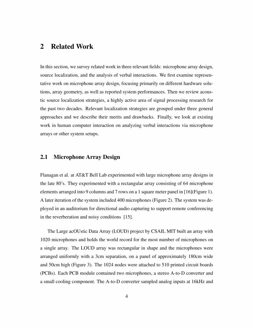
2.1 Microphone Array Design
Flanagan et al. at AT&T Bell Lab experimented with large microphone array designs in
the late 80’s. They experimented with a rectangular array consisting of 64 microphone
elements arranged into 9 columns and 7 rows on a 1 square meter panel in [16](Figure 1).
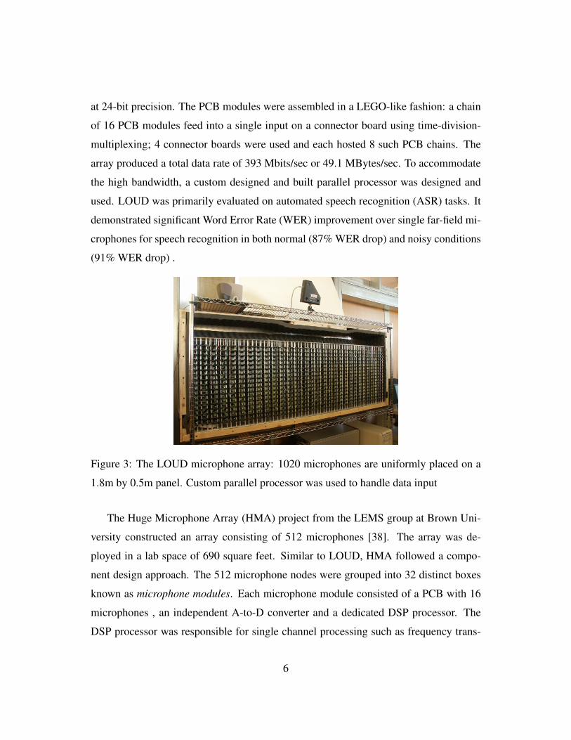
A later iteration of the system included 400 microphones (Figure 2). The system was de-
ployed in an auditorium for directional audio capturing to support remote conferencing
in the reverberation and noisy conditions [15].
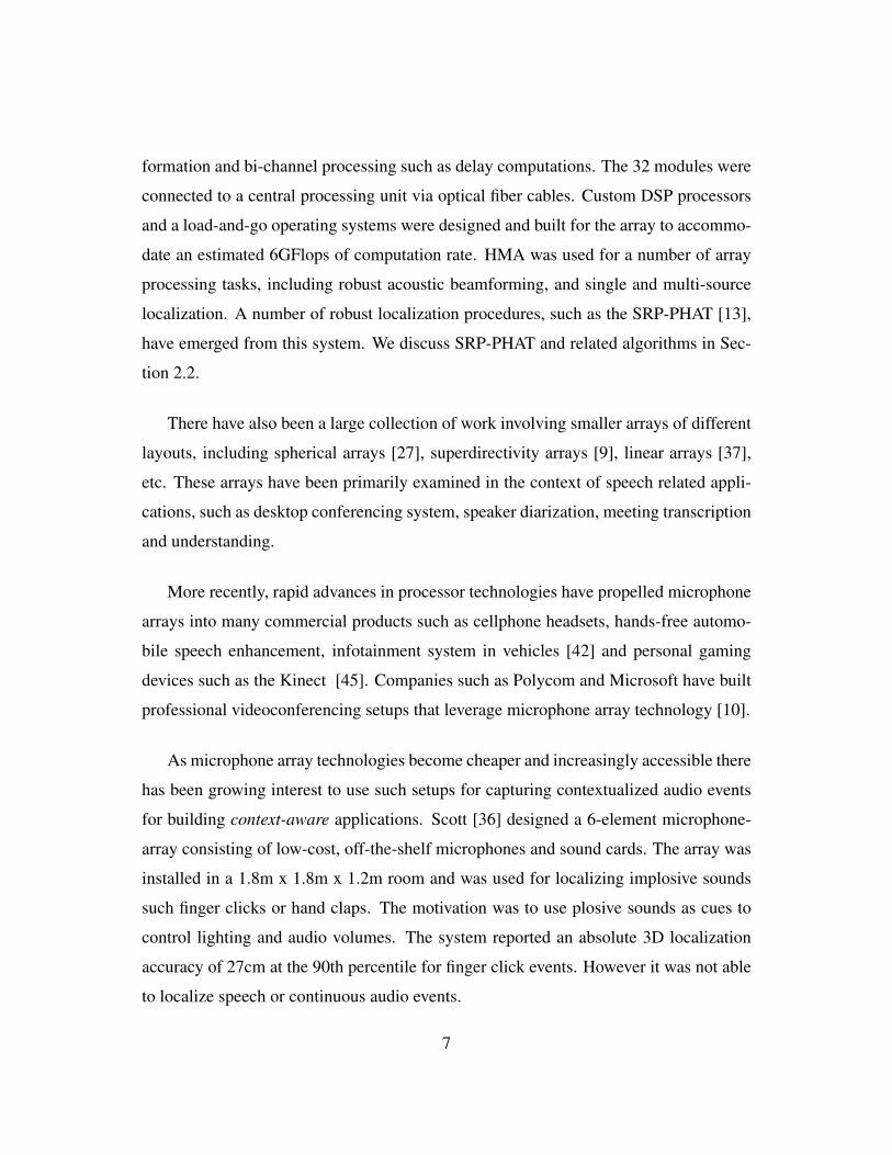
The Large acOUstic Data Array (LOUD) project by CSAIL MIT built an array with
1020 microphones and holds the world record for the most number of microphones on
a single array. The LOUD array was rectangular in shape and the microphones were
arranged uniformly with a 3cm separation, on a panel of approximately 180cm wide
and 50cm high (Figure 3). The 1024 nodes were attached to 510 printed circuit boards
(PCBs). Each PCB module contained two microphones, a stereo A-to-D converter and
a small cooling component. The A-to-D converter sampled analog inputs at 16kHz and
4
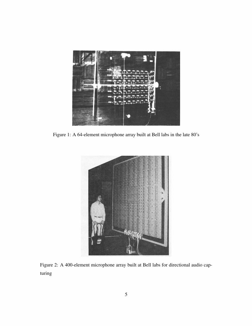
Figure 1: A 64-element microphone array built at Bell labs in the late 80’s
Figure 2: A 400-element microphone array built at Bell labs for directional audio cap-
turing
5
at 24-bit precision. The PCB modules were assembled in a LEGO-like fashion: a chain
of 16 PCB modules feed into a single input on a connector board using time-division-
multiplexing; 4 connector boards were used and each hosted 8 such PCB chains. The
array produced a total data rate of 393 Mbits/sec or 49.1 MBytes/sec. To accommodate
the high bandwidth, a custom designed and built parallel processor was designed and
used. LOUD was primarily evaluated on automated speech recognition (ASR) tasks. It
demonstrated significant Word Error Rate (WER) improvement over single far-field mi-
crophones for speech recognition in both normal (87% WER drop) and noisy conditions
(91% WER drop) .
Figure 3: The LOUD microphone array: 1020 microphones are uniformly placed on a
1.8m by 0.5m panel. Custom parallel processor was used to handle data input
The Huge Microphone Array (HMA) project from the LEMS group at Brown Uni-
versity constructed an array consisting of 512 microphones [38]. The array was de-
ployed in a lab space of 690 square feet. Similar to LOUD, HMA followed a compo-
nent design approach. The 512 microphone nodes were grouped into 32 distinct boxes
known as microphone modules. Each microphone module consisted of a PCB with 16
microphones , an independent A-to-D converter and a dedicated DSP processor. The
DSP processor was responsible for single channel processing such as frequency trans-
6
formation and bi-channel processing such as delay computations. The 32 modules were
connected to a central processing unit via optical fiber cables. Custom DSP processors
and a load-and-go operating systems were designed and built for the array to accommo-
date an estimated 6GFlops of computation rate. HMA was used for a number of array
processing tasks, including robust acoustic beamforming, and single and multi-source
localization. A number of robust localization procedures, such as the SRP-PHAT [13],
have emerged from this system. We discuss SRP-PHAT and related algorithms in Sec-
tion 2.2.
There have also been a large collection of work involving smaller arrays of different
layouts, including spherical arrays [27], superdirectivity arrays [9], linear arrays [37],
etc. These arrays have been primarily examined in the context of speech related appli-
cations, such as desktop conferencing system, speaker diarization, meeting transcription
and understanding.
More recently, rapid advances in processor technologies have propelled microphone
arrays into many commercial products such as cellphone headsets, hands-free automo-
bile speech enhancement, infotainment system in vehicles [42] and personal gaming
devices such as the Kinect [45]. Companies such as Polycom and Microsoft have built
professional videoconferencing setups that leverage microphone array technology [10].
As microphone array technologies become cheaper and increasingly accessible there
has been growing interest to use such setups for capturing contextualized audio events
for building context-aware applications. Scott [36] designed a 6-element microphone-
array consisting of low-cost, off-the-shelf microphones and sound cards. The array was
installed in a 1.8m x 1.8m x 1.2m room and was used for localizing implosive sounds
such finger clicks or hand claps. The motivation was to use plosive sounds as cues to
control lighting and audio volumes. The system reported an absolute 3D localization
accuracy of 27cm at the 90th percentile for finger click events. However it was not able
to localize speech or continuous audio events.
7
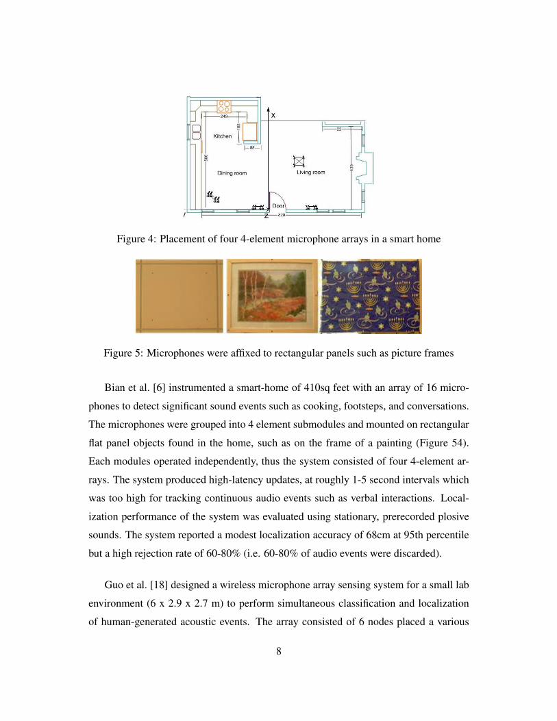
Figure 4: Placement of four 4-element microphone arrays in a smart home
Figure 5: Microphones were affixed to rectangular panels such as picture frames
Bian et al. [6] instrumented a smart-home of 410sq feet with an array of 16 micro-
phones to detect significant sound events such as cooking, footsteps, and conversations.
The microphones were grouped into 4 element submodules and mounted on rectangular
flat panel objects found in the home, such as on the frame of a painting (Figure 54).
Each modules operated independently, thus the system consisted of four 4-element ar-
rays. The system produced high-latency updates, at roughly 1-5 second intervals which
was too high for tracking continuous audio events such as verbal interactions. Local-
ization performance of the system was evaluated using stationary, prerecorded plosive
sounds. The system reported a modest localization accuracy of 68cm at 95th percentile
but a high rejection rate of 60-80% (i.e. 60-80% of audio events were discarded).
Guo et al. [18] designed a wireless microphone array sensing system for a small lab
environment (6 x 2.9 x 2.7 m) to perform simultaneous classification and localization
of human-generated acoustic events. The array consisted of 6 nodes placed a various
8
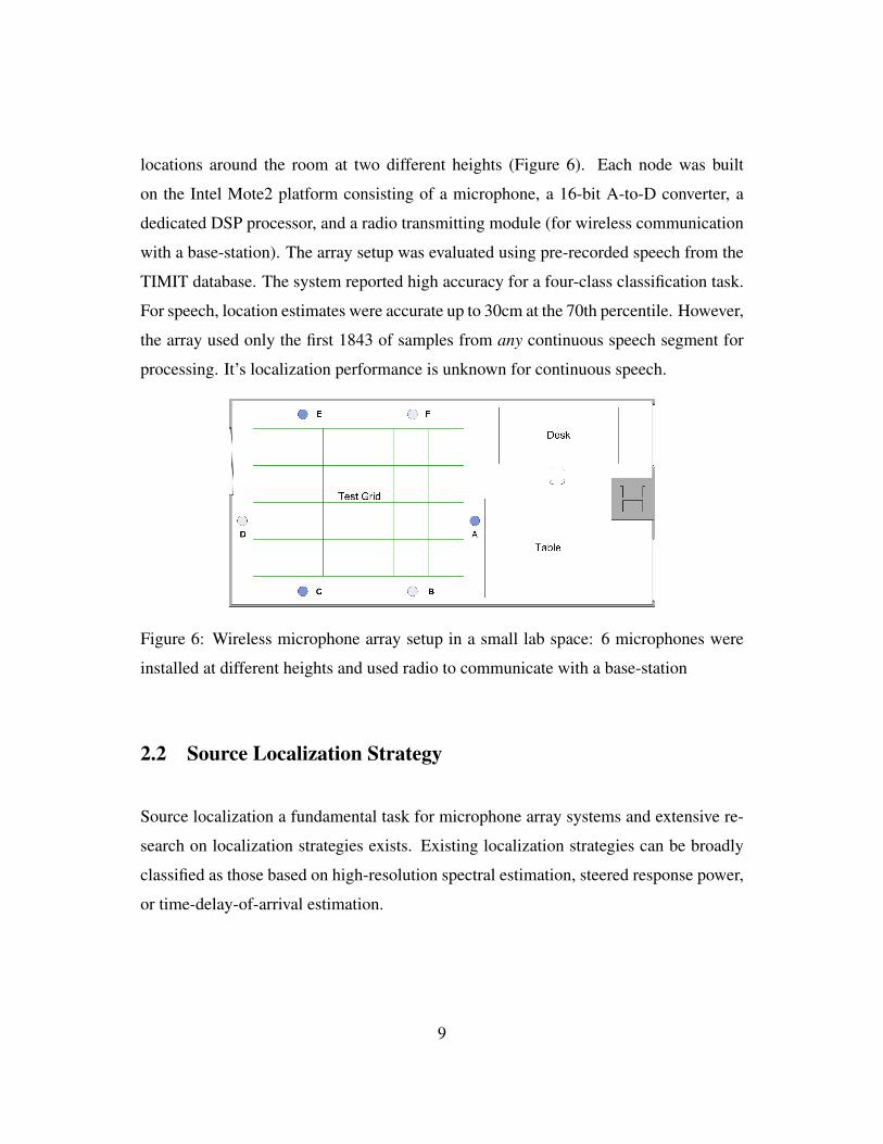
locations around the room at two different heights (Figure 6). Each node was built
on the Intel Mote2 platform consisting of a microphone, a 16-bit A-to-D converter, a
dedicated DSP processor, and a radio transmitting module (for wireless communication
with a base-station). The array setup was evaluated using pre-recorded speech from the
TIMIT database. The system reported high accuracy for a four-class classification task.
For speech, location estimates were accurate up to 30cm at the 70th percentile. However,
the array used only the first 1843 of samples from any continuous speech segment for
processing. It’s localization performance is unknown for continuous speech.
Figure 6: Wireless microphone array setup in a small lab space: 6 microphones were
installed at different heights and used radio to communicate with a base-station
2.2 Source Localization Strategy
Source localization a fundamental task for microphone array systems and extensive re-
search on localization strategies exists. Existing localization strategies can be broadly
classified as those based on high-resolution spectral estimation, steered response power,
or time-delay-of-arrival estimation.
9
2.2.1 High Resolution Spectral Estimation
High-resolution spectral estimation has its roots in narrow-band array processing tech-
niques found in antenna and sonar research, including autoregressive signal modeling,
minimum variance spectral estimation, and a family of well-known eigenanalysis meth-
ods, such as MUSIC [34], ESPRIT [33] and MIN-NORM [26]. All of these techniques
rely on the exploiting the structure and properties of the cross-sensor (spatial) spectral
covariance matrix (CSCM) estimated from observed data. Theoretically, these tech-
niques are able to resolve to multiple point sources, but their effectiveness in real-world
scenarios are limited as they make a number fundamental signal assumptions that are
difficult to meet in practice. For instance, CSCM is often estimated by ensemble av-
eraging of the received signals over a time interval in which the sources and noise are
assumed to be statistically stationary. This is difficult for speech signals because speech
can only be assumed to be stationary for very short intervals, yet longer averaging is
often needed to obtain a sufficiently accurate CSCM in noisy conditions.
The theoretical array model underlying spectral estimation is well-defined only in
the context of narrow-band signals, where the bandwidth is a small fraction of the central
frequency of the sensor passband. Hence subspace methods such as MUSIC or ESPIRIT
are of limited use for wide-band signals such as speech. Extensions to these methods
are available, for example, by splitting the array passband into multiple frequency bins
and applying narrow band algorithms to each sub-band [40], or by applying a focusing
procedure to produce a single matrix to which the narrow-band algorithm is applied [43].
While these extensions do remove the narrow-band limitation, they generally require
much higher computation requirements and tend to be less robust to source and senor
model differences.
The output of spectral estimation techniques is a collection of Direction-of-arrival
angles, which inherently assume that the source is in the far-field. Near-field extension
10
are possible but at the cost of higher computation demand [43]. Despite many of the
issues in applying high-resolution spectral estimation, they have been shown promise
for multi-source localization problems [11].
2.2.2 Steered Response Power
Steered response power (SRP) locators are based on the intuition that if one can measure
the distribution of spectral power over a 3D space, then the distribution should show
strong peaks at sound emitting locations. SRP locators borrows from beamforming
by focusing an array to various candidate locations and select the location with the
greatest power [44, 19]. One of the simplest types of SRP is the output of a delay-and-
sum beamformer. The delay-and-sum beamformer uses a simple delay structure to shift
signals relative to a reference microphone to compensate for propagation delays. These
signals are time-aligned and summed together to give a single output. The simple delay-
and-sum beamformer can be extended by applying different filters prior to the summing
procedure, leading to more general filter-and-sum beamformers.
Beamforming was traditionally used to obtain a “better” speech signal by focusing
an array to the known location of a source. Optimum beamforming algorithms are gen-
erally much more expensive than estimating the location of sources. This is justified
since beamforming only needed to be performed after the location of the sound source
had been determined. When beamforming is applied to SRP-based localizers, the loca-
tion of the source is unknown, hence array may need to focus to many candidate source
locations, each of which is associated with an expensive beamforming operation.
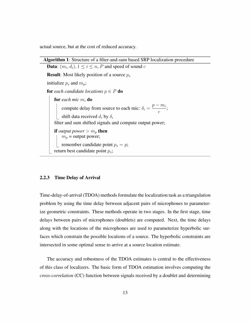
To better understand SRP-based estimators from the perspective of real-time source
localization, its basic structure is shown in Algorithm 1. For an array with n nodes,
the input to the procedure is the static microphone locations (in 3D) mi, the data frame
captured by the microphones di, for 1 ≤ i ≤ n, and a set of source candidate position
11
P in 3D. The procedure returns the most likely position of a source, where likelihood is
defined as the output-power at the hypothesized source location.
The SRP procedure iterates over candidate locations in P . P is often computed a-
priori and is a function of two variables: (1) the aperture of the array – the 3D volume
within which localization should be performed and (2) spatial resolution – the maximum
accepted spatial quantization error. P is commonly defined using one or more grids
covering the 3D aperture. As a consequence, a k-fold increase in spatial resolution
amounts to a k3 increase in computational requirement. Suppose we have a modest-sized
3D aperture of 3 x 4 x 2m (e.g. a small array equipped conference room) and a spatial
resolution of 10cm, an SRP-based localizer will require 24000 beamforming operations
per data frame. Increasing to a 5cm spatial resolution represents an 8-fold increase to
about 200000 beamforming operations. For a 1cm spatial resolution a staggering 25
million beamforming operations are needed, corresponding to a 1000 times increase.
Many beamform structures, such as the Maximum-Likelihood (ML) beamformer
require significant computation for each beamforming operation and can be computa-
tionally prohibitive for real-time localization in even modest sized rooms. Furthermore,
ML beamformers are highly dependent on the assumed spectral properties of the source
signal and background noise, and thus are less effective in practice. The SRP-PHAT al-
gorithm is a filter-sum SRP locator. It addresses robustness issues for highly reverberant
conditions by filtering the signals via PHAT weighting. Highly accurate location esti-
mates can be obtained from SRP-PHAT and it has been applied to offline location esti-
mation for a number of systems. However, a computation requirement of 2.46TeraFlops
was reported in [14], when SRP-PHAT was applied to real-time (25.6ms) localization
on a 24 element array. To reduce the computational requirement of SRP-PHAT, a more
efficient version based on stochastic region contraction was proposed in [14]. The algo-
rithm avoided brute-force grid-search by iteratively contracting the likely region for the
12
actual source, but at the cost of reduced accuracy.
Algorithm 1: Structure of a filter-and-sum based SRP localization procedureData: (mi, di), 1 ≤ i ≤ n, P and speed of sound c
Result: Most likely position of a source ps
initialize ps and mp;
for each candidate locations p ∈ P do
for each mic mi do
compute delay from source to each mic: δi =p−mi
c;
shift data received di by δifilter and sum shifted signals and compute output power;
if output power > mp thenmp = output power;
remember candidate point ps = p;return best candidate point ps;
2.2.3 Time Delay of Arrival
Time-delay-of-arrival (TDOA) methods formulate the localization task as a triangulation
problem by using the time delay between adjacent pairs of microphones to parameter-
ize geometric constraints. These methods operate in two stages. In the first stage, time
delays between pairs of microphones (doublets) are computed. Next, the time delays
along with the locations of the microphones are used to parameterize hyperbolic sur-
faces which constrain the possible locations of a source. The hyperbolic constraints are
intersected in some optimal sense to arrive at a source location estimate.
The accuracy and robustness of the TDOA estimates is central to the effectiveness
of this class of localizers. The basic form of TDOA estimation involves computing the
cross-correlation (CC) function between signals received by a doublet and determining
13
the delay with the highest correlation. Background noise and room reverberation are
two major sources of degradation for robust peak detection in the cross-correlation.
The Generalized Cross Correlation (GCC) function was proposed to improve TDOA
estimation by pre-filtering or frequency-reweighting signals before evaluating the CC
function. Many variations of GCC functions have been examined, including SCOT,
Maximum-Likelihood (ML), and GCC-PHAT [24]. The GCC-PHAT function became
widely popular due to its robustness to moderate noise and reverberation conditions.
We examine GCC-PHAT in more detail in Section 4 since it forms the basis for the
localization procedure in our system.
Given TDOA estimates, the second stage of obtaining a location estimate involves
solving a set of nonlinear equations. Various algorithms have been developed, with
varying assumptions e.g. near field vs far field source, and capabilities e.g. 2D vs.
3D localization. The solvers can either give exact solutions which are often based on
an iterative procedure or give closed-form solutions. While closed-form estimators are
cheaper to compute they give sub-optimal results by approximating the exact solution
to the nonlinear problem [35, 39].
This class of localizers are generally much more efficient than both high resolution
spectral estimation and SRP-based locators and thus are have been more widely used for
real-time localization. Despite superior performance properties, they do suffer robust-
ness issues in the presence of high reverberation and noise interference, which are not
uncommon for realistic deployment environments. The problems can be further com-
pounded by real-time, low-latency localization requirements. In addition, TDOA based
locators are formulated for single source localization and it’s not obvious how to extend
the scheme to multi-source localization. We discuss how these issues are addressed in
our system in Section 4.
14

2.3 Verbal Interaction Analysis
Conversation analysis (CA) is a well established method in sociology, anthropology, lin-
guistics and psychology to study social dynamics via verbal and nonverbal interactions.
It is particular influential in sociolinguistics and discourse analysis. More recently, there
has been growing interest in using computer assisted technologies to study conversations
and automate CA. Aoki et al [4], used a multi-microphone setup (one close-talking mic
person) to record round-table, multi-party (3+ people), co-located, social interactions.
Voice activity detection was applied to the multi-channel recording to extract turn-taking
and speaker floor information. Together with transcripts of the recording, they exam-
ined the structural and temporal aspects of casual spontaneous dialog. In particular,
they focused on the mechanics of multiple simultaneous conversational floors, how par-
ticipants initiate a new floor amidst an on-going floor (known as schisming), and how
participants subsequently show their affiliation with one floor over another. A number
of recommendations for conversation modeling was given. In particular, it was sug-
gested that to analyze real world sociable interactions a system can not only assume that
conversational participation share a single floor via dyadic behavior.
Karahalios et al. [21] created numerous real-time visualizations of on-going social
conversations. It was found that by providing feedback in the form of visualizations
of turn-taking behavior, overlapping speech and energy levels, the displays could act as
reflective mechanisms (“social mirrors”) to mitigate social tension and to help maintain-
ing social norms such as equal participation and reduced interruption. Work by Kim
et al [23] built a real-time visualization around conversational engagement using data
collected from speech, body movement and proximity. The visualization was shown to
be effective in encouraging participates to balance participation during remote confer-
encing scenarios.
Roy et al. [32] instrumented homes with eleven video cameras and fourteen-element
15
microphone arrays to obtain unobtrusive continuous recording of all activities continu-
ously for years. The data was used to understand the language acquisition process of
children by mapping the utterances over both spatial and temporal dimensions.
Choudhury et al. [8] explored the use speech prosody and Markov processes to
model and discover long-term social interactions. Speech, location, and proximity in-
formation was captured via an integrated sensing device known as the Sociometer [7].
Basu [5] created a library of robust techniques for conversation scene analysis and stud-
ied those techniques on data collected from the Sociometer. This library includes al-
gorithms for extracting low-level auditory cues, such as pitch, speaking rate, and en-
ergy, a linked HMM for detecting voiced and unvoiced regions of speech. These low
to mid-level features would then be used to segment speech signal into conversation
scenes. Conversation scenes, location data and speaker identifiers were input to vari-
ous models to try to learn the communication patterns with a community, various social
network properties, individual turn-taking style and how people influence each other’s
turn-taking style.
In his book Honest Signals, Pentland examined the predictive power of social signals
that are unconsciously communicated on the outcomes of social interactions [29]. Four
categories of honest signals were highlighted, including Influence - the extent to which
one person causes the other person’s pattern of speaking to match their own pattern,
Mimicry - the reflexive copying of one person by another during a conversation, Activity
- an indication of interest and arousal, Consistency - the emphasis and timing of speech
as a sign of mental focus. These honest signals are mapped to combinations of prosodic
features and spatial features. A series of studies using the Sociometer was carried out
to examine the effectiveness of using these features to predict the outcome of various
conversations including salary negotiation, speed dating, and VC pitch. “Thin-slice” be-
havioral analysis was used which involves analyzing a short windows of conversational
speech (e.g. the first couple of minutes) and it was found to be surprisingly predictive.
16
3 System Design
In this section we discuss the hardware and software design of of a Scalable Large
Aperture Array of Microphones (SLAAM). We start by discussing the high level design
rationales. Scalability was a key design consideration, in terms of the area covered,
density, and number of sources that can be tracked by the array. SLAAM was built
using commodity and relatively inexpensive off-the-shelf audio components. This is
an important distinction of this system compared to more common designs based on
custom manufactured hardware components. At the same time off-the-shelf modules do
impose more constraints on the design of the system, ranging from physical wiring to
computational limitation. We’ll consider these limitations as we describe our system.
3.1 Design Goals
We motivate the design of SLAAM along a number of dimensions.
• Low Cost Cost is a practical and important design criteria, but is not often consid-
ered or explicitly explained in prior work. Elaborate sensor setups are often too
costly to design and deploy, such as for homes and small meeting spaces. In this
project we set out to design a system that is relative inexpensive to build, install
and maintain.
A clear understanding of the expected cost is important to evaluate the feasibility
and scalability of a design. We can break the total cost of deploying a micro-
phone array system into the following components: hardware, installation, and
maintenance. The total cost of a system can be defined as :
total cost = cost of hardware + installation + maintenance/year × years deployed
17
Maintenance cost is generally a running cost. The sensitive region of a micro-
phone array refers to the area in which the array can produce sufficiently accurate
localization results for the applications being supported. Given a deployment en-
vironment of a specific sensitive region, one obvious cost metric is cost-per-unit-
area:
cost-per-unit-area =total cost
area of sensitive region
Under this cost model, it is desirable to increase the sensitive area (large aperture)
while using a relatively small (sparse) number of microphones.
• Commodity Hardware One of the factors which could significantly impact the
cost models above is the amount of customization required for an array design to
accommodate specific deployment requirements. Custom hardware designs are
often more configurable (e.g. dealing with wiring requirements) but typically in-
cur steeper manufacturing costs. Custom systems are also generally more brittle
with respect to hardware failures, especially during long term deployment, thus
driving up maintenance cost. In contrast, commodity hardware are generally more
solid, robust, and more thoroughly tested. For these reasons, we set out to examine
the feasibility of building a robust array system by using only off-the-shelf com-
ponents. The was system was designed to improve high replicability so someone
else can relatively easily set up a similar installation elsewhere. The hardware
components are discussed in more detailed in Section 3.2
• Low-latency localization Latency requirements for a localization service are de-
pendent on the applications being designed and supported. Take as example an
audio-based automatic camera steering application for video-conferencing sys-
tem, it is unlikely that an active audio source (participants of the conference)
will make sudden and rapid movements. Furthermore, even when movements
are present, there is rarely a need to track all instantaneous changes. As such, la-
18

tency of up to 200-300ms are very acceptable for these applications. Instead, if the
array-based localization system is to be employed as the front-end of an automatic
speech recognition (ASR) or diarization system, then position estimates must be
updated quickly, since even small misalignment or “steering errors” will signifi-
cantly degrade ASR and diarization performances. Hence for speech understand-
ing and segmentation systems, it is expected that location updates be provided on
20-50ms data frames [8, 12, 3]. However, it should be noted that “real-time” ASR
and diarization systems are rare, and the majority of these systems work offline or
in batch mode on entire segments of recorded meetings or speech. As such, these
system typically favor higher accuracy over lower latency in their design. SLAAM
was designed for real-time applications such as conversation visualization, anal-
ysis, and quasi-real-time applications such a as speech-driven applications. Thus
latency is an important design constraint.
• Multi-source localization In general, multiple simultaneous active conversations
may take place in a large physical space. When the physical separation of these
conversations are sufficiently close, microphones will receive mixtures of speech
generated by multiple simultaneous speakers (and noise sources). Thus the local-
ization algorithm cannot assume a simplistic single-speaker-only model.
While simultaneous speech is more likely to be generated between multiple con-
versations, they do occur within a conversation and are important for understand-
ing the turn-taking patterns of conversations [4]. For example, turn-stealing or
interruption is a verbal event that causes momentary simultaneous speech and is
often associated with disagreement or dominance [41]. In social conversations,
overlapping speech could also be associated with “cooperative overlap”, which
describe the case in which one speaker talks at the same time as another speaker
not in order to interrupt but to show enthusiastic listenership and participational
interest in the conversation. We discuss these patterns of speech overlap and how
they are captured by our system in Section 6.
19
• Spatial precision The spatial precision of a system is another dimension that de-
pends on the applications to be supported. For example in spatial conversation
analysis, separating the speakers is an important requirement. It has been well es-
tablished by proximics theory from social psychology that the degree of intimacy
between individuals has high correlation with physical distance during a conver-
sation, which can range from 0.5m for highly intimate conversation to 7.6 m for
public speaking [20]. The physical separation among acquaintances in a social
conversations ranges between 1.2 - 4.7 meters while the distance between good
friends and family on the average ranges from 0.5 - 1.2 meters. This suggests
that we can lower bound the physical separation between speakers by 50cm ( 20
inches). This implies that a source location estimate which deviates by more than
25cm from the true location will likely be incorrectly classified. The system will
need to produce location estimates well below this error margin.
3.2 Hardware Design
We now discuss the hardware implementation of the array system. We examine the
components used, their capabilities, and various design considerations in array place-
ment and component connectivity.
3.2.1 Components
SLAAM is constructed entirely using commodity, off-the-shelf audio modules consist-
ing of:
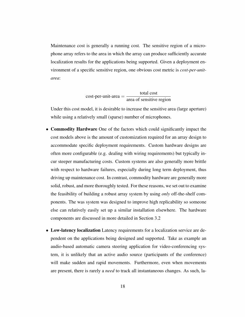
• Thirty-six Shure Easyflex Boundary microphones (Figure 7). The microphones
are omni-directional with a frequency response in the 50Hz to 17kHz range. The
20
Figure 7: The Shure Easyflex Boundary microphones
response is flat across the vocal range (300Hz - 2kHz).
• Six SMProAudio preamplification devices (Figure 8) which supports 8 TRS input
and 8 TRS outputs. The preamp provides a maximum gain of 60dB for each
discrete input channel.
• Six MOTU MKII devices with integrated digitizer, mixer, and streaming capabil-
ities (Figure 8). A single MKII digital mixer supports up to eight TRS analog
inputs. The digitizer can sample at 44.1kHz, 48kHz, or 96kHz and at 24-bit pre-
cision. Each mixer comes with two firewire 400 interfaces which support a max-
imum transfer rate of 49.15MBytes/second and a maximum connection distance
of 4.95 meters. Each module also has one set of ADAT optical light pipe connec-
tors that can be used to stream up to 8 channels of 44.1/48kHz audio between two
connected MKII modules.
• A Dell Quad-core i5-2.8GHz workstation.
21

Figure 8: A preamp plus digital mixer module
Figure 9: Adjacent pairs of MKIIs are connected by ADAT light pipes. Odd-numbered
MKII modules are daisy chained.
22
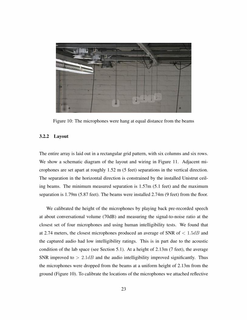
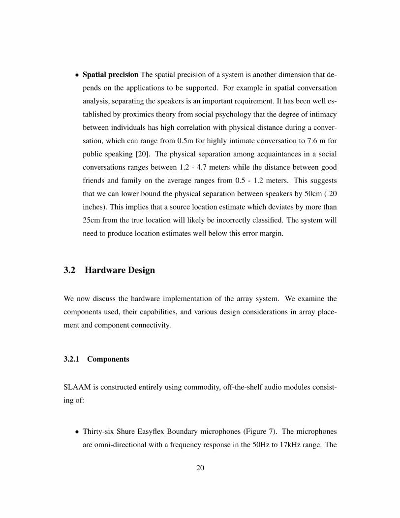
Figure 10: The microphones were hang at equal distance from the beams
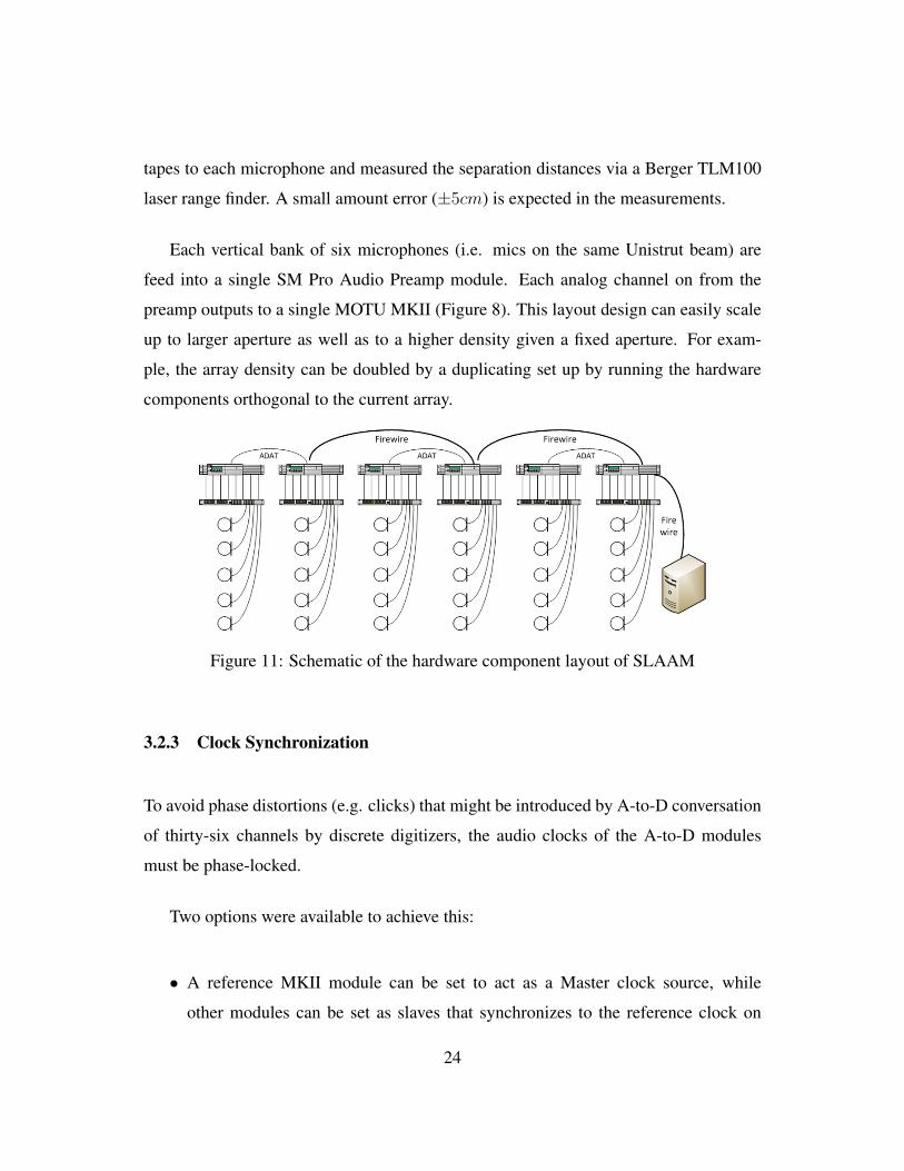
3.2.2 Layout
The entire array is laid out in a rectangular grid pattern, with six columns and six rows.
We show a schematic diagram of the layout and wiring in Figure 11. Adjacent mi-
crophones are set apart at roughly 1.52 m (5 feet) separations in the vertical direction.
The separation in the horizontal direction is constrained by the installed Unistrut ceil-
ing beams. The minimum measured separation is 1.57m (5.1 feet) and the maximum
separation is 1.79m (5.87 feet). The beams were installed 2.74m (9 feet) from the floor.
We calibrated the height of the microphones by playing back pre-recorded speech
at about conversational volume (70dB) and measuring the signal-to-noise ratio at the
closest set of four microphones and using human intelligibility tests. We found that
at 2.74 meters, the closest microphones produced an average of SNR of < 1.5dB and
the captured audio had low intelligibility ratings. This is in part due to the acoustic
condition of the lab space (see Section 5.1). At a height of 2.13m (7 feet), the average
SNR improved to > 2.1dB and the audio intelligibility improved significantly. Thus
the microphones were dropped from the beams at a uniform height of 2.13m from the
ground (Figure 10). To calibrate the locations of the microphones we attached reflective
23
tapes to each microphone and measured the separation distances via a Berger TLM100
laser range finder. A small amount error (±5cm) is expected in the measurements.
Each vertical bank of six microphones (i.e. mics on the same Unistrut beam) are
feed into a single SM Pro Audio Preamp module. Each analog channel on from the
preamp outputs to a single MOTU MKII (Figure 8). This layout design can easily scale
up to larger aperture as well as to a higher density given a fixed aperture. For exam-
ple, the array density can be doubled by a duplicating set up by running the hardware
components orthogonal to the current array.
Figure 11: Schematic of the hardware component layout of SLAAM
3.2.3 Clock Synchronization
To avoid phase distortions (e.g. clicks) that might be introduced by A-to-D conversation
of thirty-six channels by discrete digitizers, the audio clocks of the A-to-D modules
must be phase-locked.
Two options were available to achieve this:
• A reference MKII module can be set to act as a Master clock source, while
other modules can be set as slaves that synchronizes to the reference clock on
24

the firewire interface.
• Use a dedicated clock source hardware. The SPIF interface on the digitizer can
be used to synchronize with the dedicated clock.
From a scalability standpoint, the first option was more appealing since (1) the clock
source would limit the number of MKII modules that can be physically attached (2) the
locations of the digitizers would be restricted by the location of the clock source due to
wiring constraints and the total coverage of the array will be limited as a result.
There is however one challenge to synchronizing the digitizers on the firewire in-
terface: a maximum of four MKII modules can be daisy-chained on a single Firewire
400 bus. We used six MKIIs to ensure that the entire deployment space was adequately
covered. To circumvent this constraint, we connected each pair of MKII modules on
their ADAT interfaces via optical light-pipes (Figure 9). The ADAT interface allows the
content of one (out) unit to be “mixed” on to the audio bus of the second (in) unit. Thus,
a pair of MKIIs are effectively processed as a single virtual unit. Clock synchronization
of all six modules can then be achieved by daisy chaining every other unit. Finally, the
master clock MKII module streams the content from its firewire interface to the server
machine’s Firewire card. To the host processing driver, only three virtual units are visi-
ble on the Firewire bus, but each unit has 12 audio channels rather than 6.
3.2.4 Cost
At the time of its construction (48 months ago), equipment cost of SLAAM was ap-
proximately $1270 per bank of mics, with the following breakdown: $750 per MKII,
$200 per preamp, $50 × 6 for the microphone nodes. Including the workstation, the
total equipment cost amounts to $8920. The quoted installation price averages to $30
per mic, due to retrofitting to an existing ceiling. A one-time calibration took place
25
post-installation and no calibration had been needed since. The hardware has also been
very resilient to failure – no mic or streaming device failure has been detected since
installation. Under our cost model we have:
cost-per-unit-area =$8920 + 1080
1000 sq ft= $10sqft
which is comparable to cost of installing office carpeting the same area.
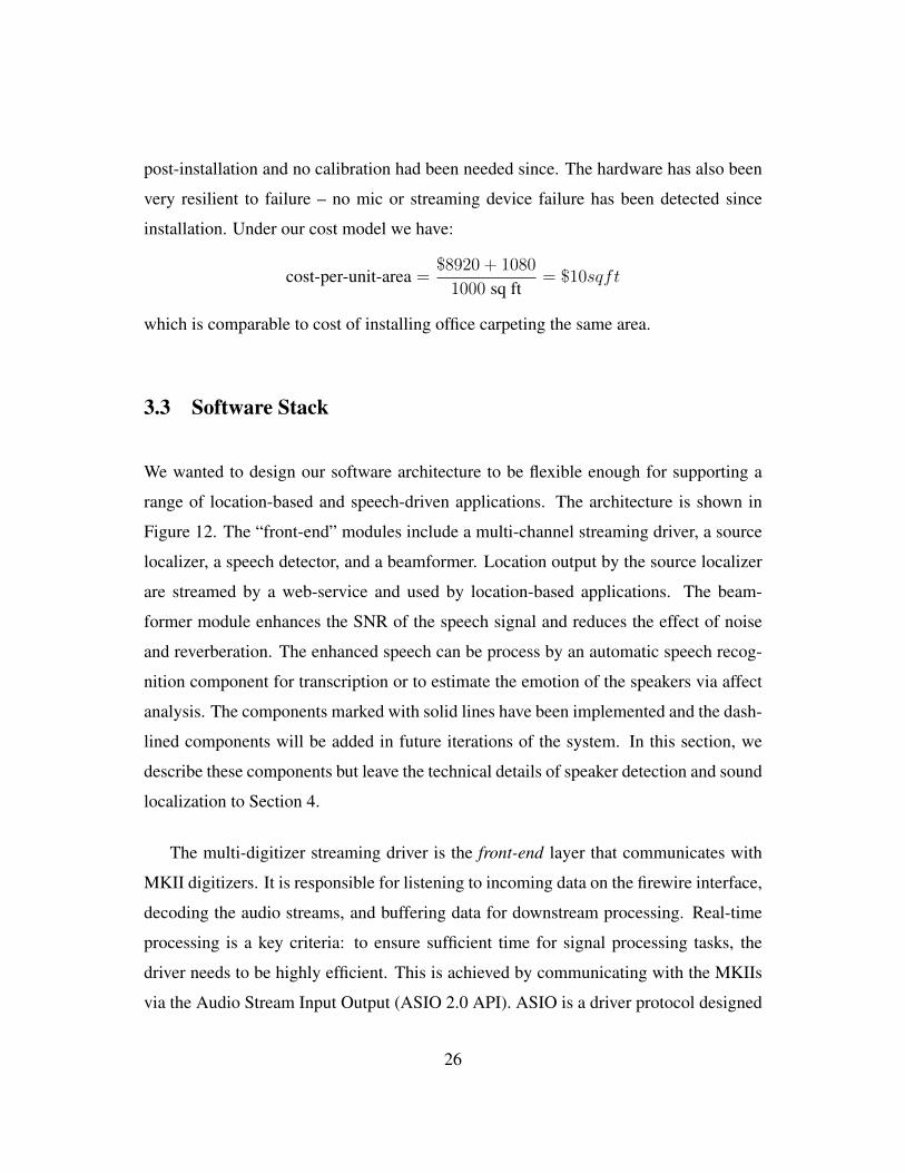
3.3 Software Stack
We wanted to design our software architecture to be flexible enough for supporting a
range of location-based and speech-driven applications. The architecture is shown in
Figure 12. The “front-end” modules include a multi-channel streaming driver, a source
localizer, a speech detector, and a beamformer. Location output by the source localizer
are streamed by a web-service and used by location-based applications. The beam-
former module enhances the SNR of the speech signal and reduces the effect of noise
and reverberation. The enhanced speech can be process by an automatic speech recog-
nition component for transcription or to estimate the emotion of the speakers via affect
analysis. The components marked with solid lines have been implemented and the dash-
lined components will be added in future iterations of the system. In this section, we
describe these components but leave the technical details of speaker detection and sound
localization to Section 4.
The multi-digitizer streaming driver is the front-end layer that communicates with
MKII digitizers. It is responsible for listening to incoming data on the firewire interface,
decoding the audio streams, and buffering data for downstream processing. Real-time
processing is a key criteria: to ensure sufficient time for signal processing tasks, the
driver needs to be highly efficient. This is achieved by communicating with the MKIIs
via the Audio Stream Input Output (ASIO 2.0 API). ASIO is a driver protocol designed
26
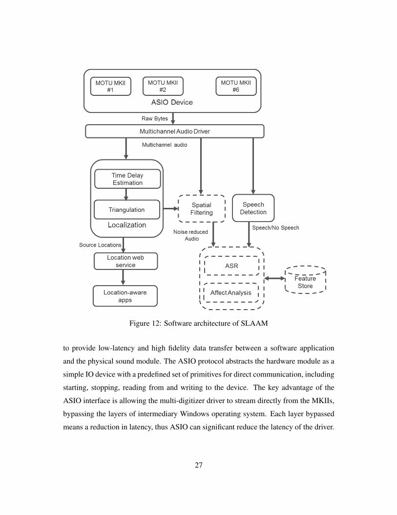
Figure 12: Software architecture of SLAAM
to provide low-latency and high fidelity data transfer between a software application
and the physical sound module. The ASIO protocol abstracts the hardware module as a
simple IO device with a predefined set of primitives for direct communication, including
starting, stopping, reading from and writing to the device. The key advantage of the
ASIO interface is allowing the multi-digitizer driver to stream directly from the MKIIs,
bypassing the layers of intermediary Windows operating system. Each layer bypassed
means a reduction in latency, thus ASIO can significant reduce the latency of the driver.
27
The ASIO-based streaming driver uses call-backs to signal relevant hardware events.
For example, when the hardware buffer is filled, a predefined call-back method will be
invoked. The driver is responsible to interpreting and processing this data. We remarked
in Section 3.2 that the minimum sampling frequency of MKII is 44.1kHz. The MKIIs
also support four different sized hardware buffers: 258, 512, 1024, and 2048 samples.
Under 44.1KHZ sampling, this means that the internal hardware buffers will be full
in 12.9ms 23.8ms, 47.6ms, 96.2ms, 192.4ms, corresponding to the different hardware
buffer sizes.
To support real-time processing, MKIIs use a simple double internal buffering strat-
egy. That is, an MKII will reserve two equal length buffers A and B. Data buffering
will start from buffer A and once buffer A is filled, ASIO signals the driver to process
that data frame. While A is in use, MKII continues to buffer incoming data on buffer
B. When B is filled, the call-back is invoked again and the roles of the buffers are now
switched. This is depicted in Figure 13, where blue is used to denote the buffer being
processed by the driver and green is used to denote the buffer currently storing incom-
ing data. This configuration also means that the driver must finish processing the blue
buffer before the green buffer is filled, otherwise the previous data frame will be over-
written with new content. The combined latency of the driver and downstream DSP
must not exceed the buffering capability of the device: for a 1024 internal buffer this
maximum combined latency is 23.8ms. A semaphore is used to weakly synchronize the
ASIO device and the driver. The semaphore is set in the ASIO “data-available” call-
back function to signal the driver. The driver clears the semaphore after the current data
frame has been processed.
Figure 13: Double internal buffering scheme used by MKII
28
The beamforming module uses the output of the localization procedure (i.e. source
locations), the speaker detection module (i.e. speech or non-speech) to perform spatial
filtering of the multichannel audio input. The localization and speaker detection mod-
ules run parallel to each other (see Section 4) and are implemented in C++ using the
Intel Math Kernel Library (MKL). MKL contains a collection of highly tuned and ro-
bust linear algebra routines from LAPACK.The output of the localization module are
buffered by a location service. The location service module is a daemon that listens
for incoming client connections at a public IP. Clients communicate with the daemon
via TCP/IP sockets via a simple protocol with four commands (join, quit, start, pause).
After the “start” command has been called by a connected client, the daemon starts
relaying location estimates to the clients in real-time. The clients can perform further
application specific processing (e.g. source clustering, Kalman filtering). The “pause”
commands allows clients to instruct the daemon to temporarily pause location streaming
when location estimates are being generated a faster rate than the client can handle. The
buffered location estimates are flushed and archived to persistent storage periodically.
29
4 Source Detection and Localization
In this section we examine the algorithmic details of the speech detection and source
localizations modules. We look at the way SLAAM is partitioned logically to divide the
aperture into smaller regions of submarrays. We discuss a simple, spectral divergence
based voice-activity detection (VAD) algorithm and describe in detail a two-stage lo-
calization procedure based on TDOA estimation extended from GCC-PHAT and a fast
triangulation solution.
4.1 Subarray Partitioning
The physical grid layout of the array discussed in Section 3.2.2 offers a natural partition-
ing of the array aperture into 25 non-overlapping rectangular cells. Under this scheme,
each cell is enclosed by four adjacent microphones (in both horizontal and vertical di-
rections), known as a a quad (Figure 14).
The spatial partitioning of a large aperture array can help improving the robustness
of localization for both single and multiple source localization tasks. By using a non-
overallping design, each cell can be configured to monitor only those sound sources that
are active with in its boundaries. The localization task for the full array can be broken
down into 25 independent localization tasks with 25 smaller sub-arrays. For a single
source scenario, in a large apeture array most of the channels (mics) are too far away
from the source to contain useful information for localization or beamforming tasks.
Thus the partition can be used to naturally select channels that contain the most relevant
signals and significantly reduce computational requirement by filtering out less pertinent
channels. For the multiple source case, the spatial partition effectively limits the number
of sources that need to be tracked by each sub-array. This is important for peak selec-
tion based multi-source localization strategies. As we shall see in Section 4.4, the peak
30
selection procedure examines possible combinations of peaks generated by each micro-
phone pair; the total number combinations of peaks that need to be examined grows
exponentially with the number of sources and the number of delays: O(nk) where n
is the number of sources and k is the number of delays. Further more the number of
delays is combinatorial k =(m2
), where m is the total number of single channels. For
quad-based sub-array localization the number single channels is limited to 4, i.e. k = 6.
In addition, the number of active sources that fall within the boundary of a sub-array is
physically limited by the size spatial region and the natural physical separation (prox-
imics) between people involved in conversations. In addition, from the standpoint of
beamforming, with the exception of simple delay-and-sum beamformers, most other
structures require joint optimization of multiple filter parameters which increases super-
linearly with the number of channels.
While the quad structure mimics the physical layout of the array, the partitioning of
the array into subarrays is inherently logical and it is possible to construct other regular
shaped partitioning of the space. For example, one can defining any k by k grid of
microphones as a cell (for k > 2) to increase the number of microphones in a subarray
(Figure 14). It will be interesting to study the trade-off between higher complexity
versus performance using different array layouts. In SLAAM however, we found in
calibration that for a speech source at conversational volume, microphones in adjacent
cells do not obtain signals with sufficiently high signal-to-noise ratio (i.e > 1.2dB).
Thus the current design uses a quad-based subarray partitioning scheme.
4.2 Speech Detection
To detect the presence of speech sources, we make use of an efficient voice activity de-
tector (VAD) algorithm similar to [31, 30]. The detector produces a binary classification
of a data frame xt(n) at time t as either speech or non-speech. The metric is based on
31
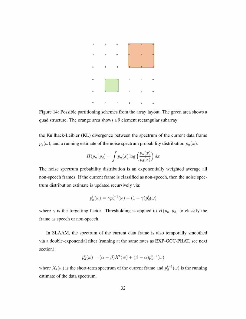
Figure 14: Possible partitioning schemes from the array layout. The green area shows a
quad structure. The orange area shows a 9 element rectangular subarray
the Kullback-Leibler (KL) divergence between the spectrum of the current data frame
pd(ω), and a running estimate of the noise spectrum probability distribution pn(ω):
H(pn‖pd) =
∫pn(x) log
(pn(x)
pd(x)
)dx
The noise spectrum probability distribution is an exponentially weighted average all
non-speech frames. If the current frame is classified as non-speech, then the noise spec-
trum distribution estimate is updated recursively via:
ptn(ω) = γpt−1n (ω) + (1− γ)ptd(ω)
where γ is the forgetting factor. Thresholding is applied to H(pn‖pd) to classify the
frame as speech or non-speech.
In SLAAM, the spectrum of the current data frame is also temporally smoothed
via a double-exponential filter (running at the same rates as EXP-GCC-PHAT, see next
section):
ptd(ω) = (α− β)X t(w) + (β − α)pt−1d (w)
where Xt(ω) is the short-term spectrum of the current frame and pt−1d (ω) is the running
estimate of the data spectrum.
32
To determine if a quad enclosure contains a speech source, VAD is applied to each of
the microphone channels independently to produce four binary outputs v1, . . . , v4. Next
we applied quad-level majority voting to decide if delay estimation and triangulation
should be attempted within the quad (ie. v1 + v2 + v3 + v4 > 2, more than two channels
are classified as speech). A minimum of three (out of four) channels need to be classified
as speech since that’s the minimum number of time delays needed for triangulation (see
Section 4.6).
Note that the VAD algorithm depends entirely on running estimates of the data and
noise spectra. From an implementation standpoint, this is efficient and fits well with
generalized cross correlation (GCC) time delay estimation algorithms that we describe
next.
4.3 Time Delay of Arrival Estimation
Given the quad partitioning of the SLAMM aperture, the delay estimation module com-
putes time-delays between any two adjacent pairs of microphones: horizontal, vertical,
and diagonal, leading to six such TDOA estimates. The time-delays estimates are not
linearly independent (some delays are completely determined by combinations of oth-
ers). However, the redundancy helps to reduces the variance of the location estimates
in the presence of estimation errors. In addition, the redudant delays can be effectively
used in a peak selection procedure and in the context of multi-source localization, as we
describe in Section 4.4.
The time delay of arrival (TDOA) estimation in SLAAM is based on GCC-PHAT.
The General Cross-Correlation (GCC) with Phase-transform (PHAT) is a well-known
technique for estimating time-delays [24]. GCC based delay estimators assume the
following signal model: a source signal x(t) is located at an unknown point p in 3D
33

space, a pair of microphones located at m1 and m2 receive delayed and noise corrupted
replicas of x(t):
x1(t) = x(t− τ1) + n1(t)
x2(t) = x(t− τ2) + n2(t)
where n1(t) and n2(t) are additive channel noises, assumed to be Gaussian and un-
correlated with x(t) and each other, τ1 and τ2 are the absolute propagation delays of
sound from p to m1 and m2 in air. The true relative delay between the received signals
is then τ12 = τ1 − τ2. By definition, the cross correlation between x1(t) and x2(t) is:
c(τ) =
∫ ∞−∞
x1(t)x2(t+ τ) dt
The GCC function is defined as the cross correlation of two filtered versions of x1(t)
and x2(t).
c(τ) =
∫ ∞−∞
(h1(x) ∗ x1(t))(h2(x) ∗ x2(t+ τ)) dt
A computationally efficient implementation of the GCC function is by transforming the
input to the frequency domain, as
R(τ) = IDFT(
Ψ12(ω)X1(ω)X∗2 (ω))
where X1(ω), X2(ω) are the spectra of the input signals, ∗ is the complex conjugation
operator, and Ψ12 is a suitably chosen weighting function. The goal of Ψ12 is to max-
imize the GCC function at R(τ) at the true delay τ12. Finally, the estimated delay is
obtained via
τ12 = arg maxτ∈D
R(τ)
whereD is the plausible interval of delays, commonly defined by the distance separating
the doublet. The GCC-PHAT is essentially a weighting function Ψ12 defined as:
Ψ12 =1
|X1(ω)X∗2 (ω)|
34
GCC-PHAT is well-known for its simplicity and efficient implementation, and has
been shown to provide fair localization accuracy under a range of acoustic conditions.
For instance, Guo et al.[18] applied the GCC-PHAT procedure to the first voiced 204.3ms
frame, or 8376 samples, of a continuous speech segment to obtain an absolute TDOA
accuracy of 60cm at 70% of the time, though errors can be as high as 2.5meters. While
these results are encouraging, it is unclear how well GCC-PHAT can consistently and
accurately produce TDOA estimates for continuous speech in a low-latency setting (e.g.
data frames of 1024 samples). In fact our experiments suggests that when applied over
an entire segment of multiple frames of speech, one might be much less optimistic about
GCC-PHAT in its basic form.
We conducted delay-estimation experiments using the TIMIT test dataset (see Sec-
tion 5.2). Given a quad, the GCC-PHAT function is computed for each doublet on
frame-by-frame basis over the entire speech segment, producing six time-series of delay
estimates. A hamming window was applied to each data frame of 1024 samples (with a
50% overlap). As shown in Figure 15, GCC-PHAT only achieved an absolute error of
60cm about 40% of the time.
GCC-PHAT is a frequency domain technique, and when applied to isolated frames
of speech data yields suboptimal TDOA estimates. In our work, we observed that the rel-
ative time-delays change only slowly over time for both stationary and even slowly mov-
ing sources. To track temporally slow varying TDOAs, we apply a double-exponential
filter over the short-term GCC-PHAT spectrum. This procedure, which we call EXP-
GCC-PHAT, takes the conventional PHAT-weighted cross-spectrum at time t: GCCt and
recursively smooths the estimate via a weighted moving average:
GCCtα = (αGCCt−1
α ) + (1− α)GCCt
GCCtβ = (βGCCt−1
β ) + (1− β)GCCt
GCCt = GCCtα − GCCt
β
35
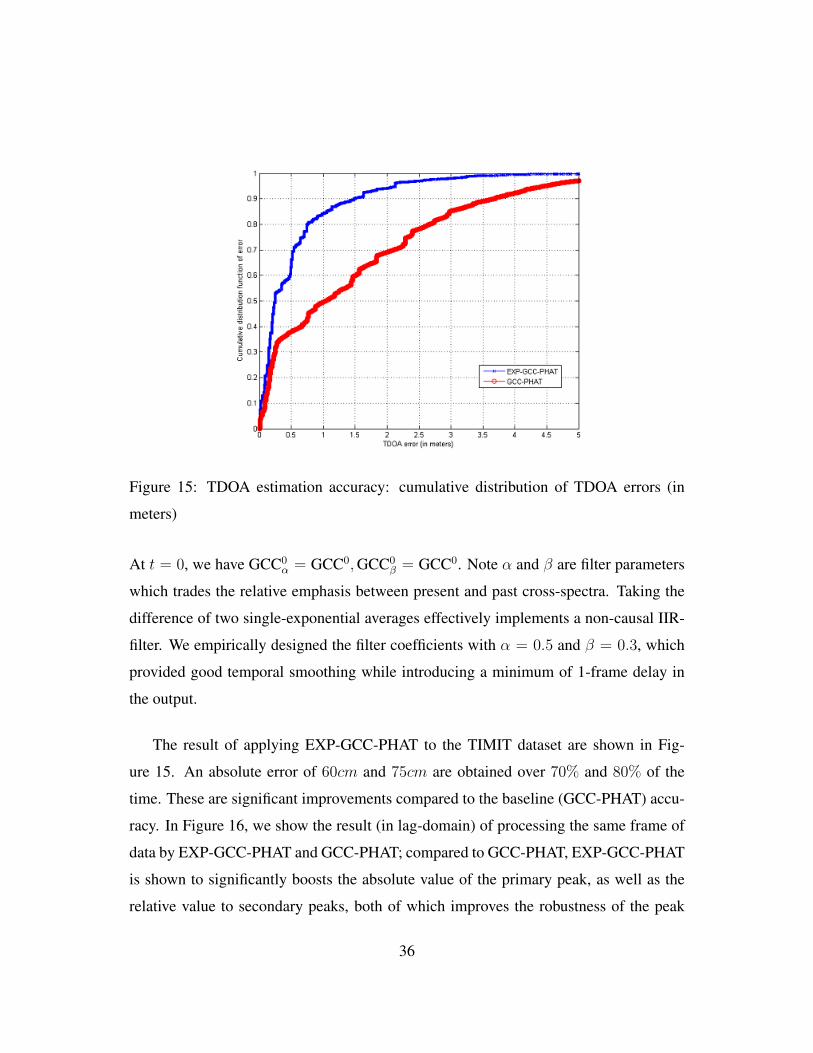
Figure 15: TDOA estimation accuracy: cumulative distribution of TDOA errors (in
meters)
At t = 0, we have GCC0α = GCC0,GCC0
β = GCC0. Note α and β are filter parameters
which trades the relative emphasis between present and past cross-spectra. Taking the
difference of two single-exponential averages effectively implements a non-causal IIR-
filter. We empirically designed the filter coefficients with α = 0.5 and β = 0.3, which
provided good temporal smoothing while introducing a minimum of 1-frame delay in
the output.
The result of applying EXP-GCC-PHAT to the TIMIT dataset are shown in Fig-
ure 15. An absolute error of 60cm and 75cm are obtained over 70% and 80% of the
time. These are significant improvements compared to the baseline (GCC-PHAT) accu-
racy. In Figure 16, we show the result (in lag-domain) of processing the same frame of
data by EXP-GCC-PHAT and GCC-PHAT; compared to GCC-PHAT, EXP-GCC-PHAT
is shown to significantly boosts the absolute value of the primary peak, as well as the
relative value to secondary peaks, both of which improves the robustness of the peak
36
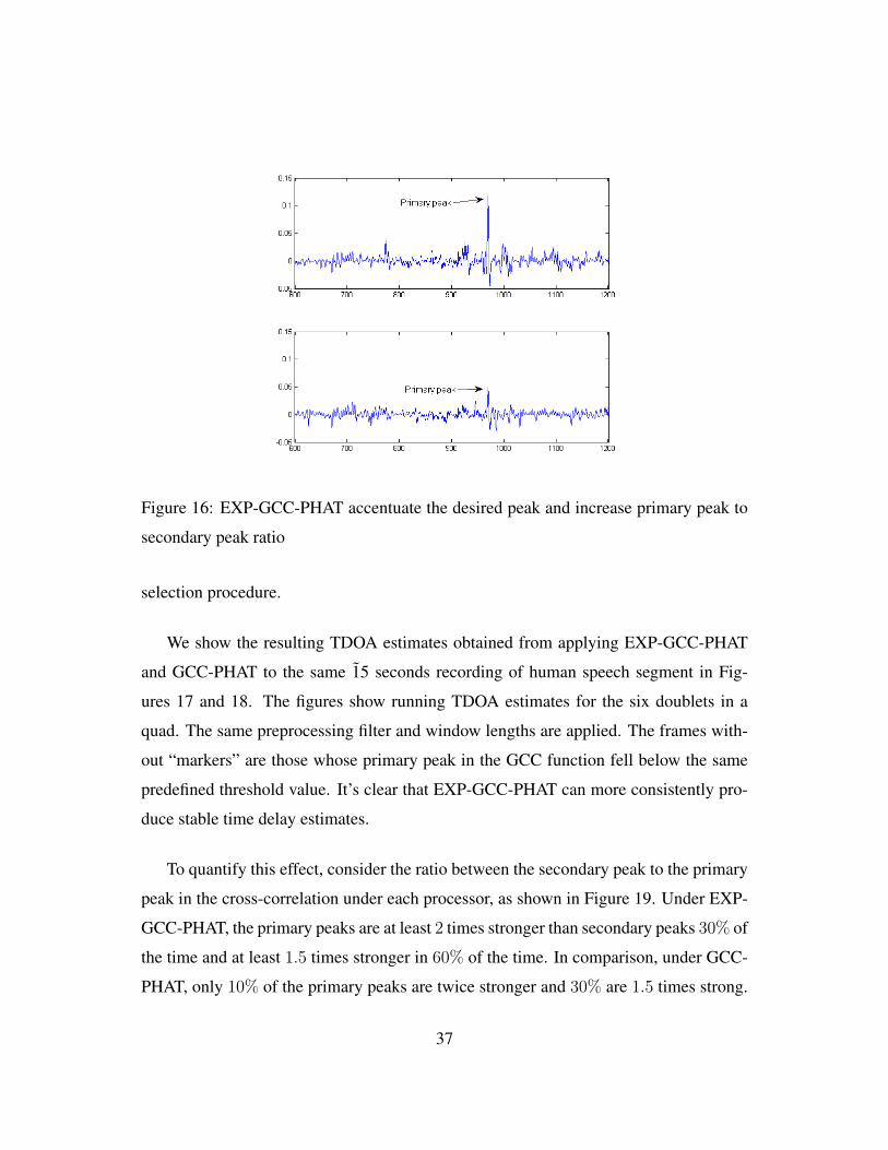
Figure 16: EXP-GCC-PHAT accentuate the desired peak and increase primary peak to
secondary peak ratio
selection procedure.
We show the resulting TDOA estimates obtained from applying EXP-GCC-PHAT
and GCC-PHAT to the same 15 seconds recording of human speech segment in Fig-
ures 17 and 18. The figures show running TDOA estimates for the six doublets in a
quad. The same preprocessing filter and window lengths are applied. The frames with-
out “markers” are those whose primary peak in the GCC function fell below the same
predefined threshold value. It’s clear that EXP-GCC-PHAT can more consistently pro-
duce stable time delay estimates.
To quantify this effect, consider the ratio between the secondary peak to the primary
peak in the cross-correlation under each processor, as shown in Figure 19. Under EXP-
GCC-PHAT, the primary peaks are at least 2 times stronger than secondary peaks 30% of
the time and at least 1.5 times stronger in 60% of the time. In comparison, under GCC-
PHAT, only 10% of the primary peaks are twice stronger and 30% are 1.5 times strong.
37
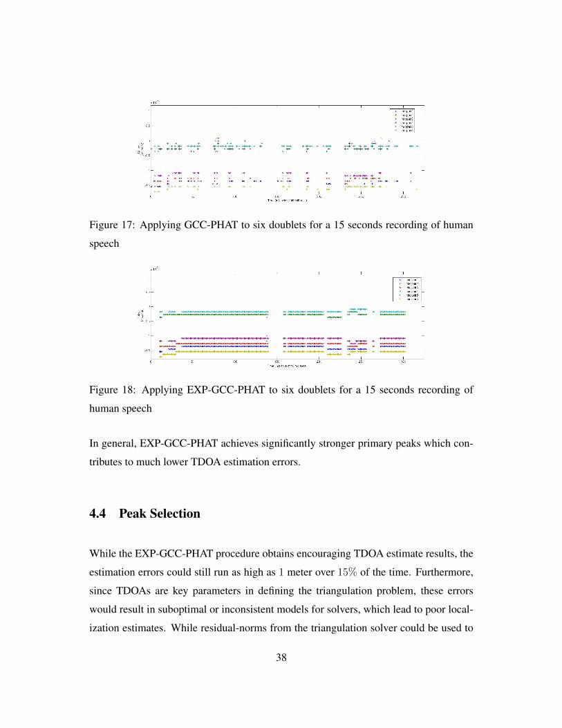
Figure 17: Applying GCC-PHAT to six doublets for a 15 seconds recording of human
speech
Figure 18: Applying EXP-GCC-PHAT to six doublets for a 15 seconds recording of
human speech
In general, EXP-GCC-PHAT achieves significantly stronger primary peaks which con-
tributes to much lower TDOA estimation errors.
4.4 Peak Selection
While the EXP-GCC-PHAT procedure obtains encouraging TDOA estimate results, the
estimation errors could still run as high as 1 meter over 15% of the time. Furthermore,
since TDOAs are key parameters in defining the triangulation problem, these errors
would result in suboptimal or inconsistent models for solvers, which lead to poor local-
ization estimates. While residual-norms from the triangulation solver could be used to
38

Figure 19: Secondary peak to primary peak ratio
evaluate the quality of a set of localization estimates, solving for the model in the first
place makes it an expensive peak quality evaluation procedure.
Furthermore, in most indoor residential or office enclosures, hard objects such as
walls, windows, and furniture will cause reflections and reverberations. These lead to
multipath propagation of the signal and will manifest as false peaks in the GCC. To ac-
count for possible strong reflections, we consider simultaneously a number of candidate
peaks. This can be accomplished by softening the requirement to return the lag which
maximizes the GCC function but rather consider the top k peaks in the GCC (which is
slower than max by a factor of only log n)
With up to k candidate peaks returned per GCC function (for a single doublet), the
39

resulting problem is a matching problem – for d doublets involved in the localization
procedure, determining which of kd possible combinations are plausible as the location
of the source. While the problems appears to combinatorial and should cause scalability
concerns, good heuristics exist to signficantly trim the problem space.
m2 m3
m4m1
d3
d4
τ12 =d1−d2
c
τ23 =d2−d3
c
d2
d1
τ13 =d1−d3
c= τ12 + τ23
Figure 20: TDOA consistency constraints
We observe that if the source location is known, then the true TDOAs can be com-
puted given the locations of the microphones. These TDOAs are also related a set of
deterministic relations. Consider Figure 20, letting di denote the distance between the
source to mic i and τi = di/c, we have the following relations:
τ12 = τ1 − τ2
τ23 = τ2 − τ3
τ13 = τ1 − τ3 = τ12 + τ23
where the last relation shows that τ13 is linearly dependent on the two other delays τ12
are τ23. We can in fact write six such relations that must be satisfied by any given set of
true TDOAs.
Viewed differently, for an unknown source with a given set of estimated TDOAs,
40

in the presence with estimation errors these relations can be seen as a metric to evalute
how close a collection of estimated TDOAs are to the true TDOAs corresponding to
some source (or strong reflection). For the relation above we define a corresponding
consistency metric:
τ13 = τ12 + τ23 + ε
for some suitably chosen threshold ε. That is, given τ13, τ12, τ23, if τ13 − τ12 − τ23 < ε
we deem the estimated delays to be consistent, otherwise they are not.
From a computational stand-point, these metrics can be evaluated efficiently with-
out traversing the complete candidate space. Observe that each consistency metric only
requires knowing three (rather than all six delays). Failure to satisfy a condition al-
lows us to prune the candidate space (for example, by eliminating all sets containing
τ13, τ12, τ23), thus avoiding generating and evaluate all k6 combinations.
We show the effectiveness of this peak selection procedure for TDOA estimation of
a single source in a reverberant room. Figure 21 shows the TDOA running estimates for
a single doublet. It’s clear that the global maximum peak “jumps” between two TDOAs,
where one corresponds to a strong reflection from a fixed brick-wall. The result after
applying peak selection is shown in Figure 22. We can see that the procedure was
effective in filtering out the strong reflection source.
Figure 21: The TDOA running estimate for a single doublet before peak selection. The
jumps between TDOA values indicates a strong reflection.
41

Figure 22: The TDOA running estimate for the same doublet after peak selection. The
strong reflection is filtered out.
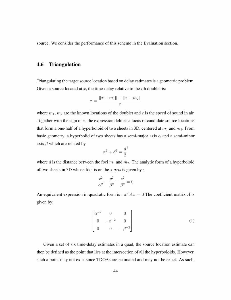
A lower bound on ε obtained by considering the best-case delay estimator, where
the estimation error ε is zero. Since the actual delays are continuous time quantities,
discretization in the lag domain introduces an uncertainty bounded by the sampling
period 1/f . We evaluate the effectiveness of this matching algorithm with respect to
error CDF by varying the threshold ε in multiples of 1/f . We performed thresholding
in an OR-fashion, i.e. the entire frame of array data is rejected if any of the d peaks
(time-delays) fails the consistency check. We see an absolute error of 3cm is achieved
at the 99th percentile (for ε = 1/f ) at a surprisingly reasonable rejection rate of around
20%. At 5% rejection rate (ε = 3/f ), 99% of errors are below 7cm.
In theory only three pairs of TDOA estimates are require for triangulating targets in
3D – however the inclusion redundant constraints will generally improve accuracy and
reduce variance in the presence of noisy estimates. In future work, we will study and
quantify the performance of less aggresive schemes by varying the number of consistent
TDOAs between 3 and 6.
42
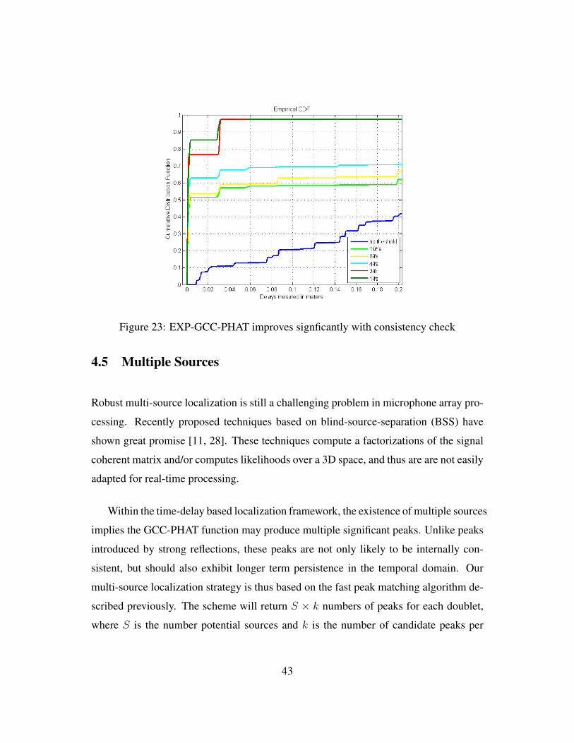
Figure 23: EXP-GCC-PHAT improves signficantly with consistency check
4.5 Multiple Sources
Robust multi-source localization is still a challenging problem in microphone array pro-
cessing. Recently proposed techniques based on blind-source-separation (BSS) have
shown great promise [11, 28]. These techniques compute a factorizations of the signal
coherent matrix and/or computes likelihoods over a 3D space, and thus are are not easily
adapted for real-time processing.
Within the time-delay based localization framework, the existence of multiple sources
implies the GCC-PHAT function may produce multiple significant peaks. Unlike peaks
introduced by strong reflections, these peaks are not only likely to be internally con-
sistent, but should also exhibit longer term persistence in the temporal domain. Our
multi-source localization strategy is thus based on the fast peak matching algorithm de-
scribed previously. The scheme will return S × k numbers of peaks for each doublet,
where S is the number potential sources and k is the number of candidate peaks per
43
source. We consider the performance of this scheme in the Evaluation section.
4.6 Triangulation
Triangulating the target source location based on delay estimates is a geometric problem.
Given a source located at x, the time-delay relative to the ith doublet is:
τ =‖x−m1‖ − ‖x−m2‖
c
where m1, m2 are the known locations of the doublet and c is the speed of sound in air.
Together with the sign of τ , the expression defines a locus of candidate source locations
that form a one-half of a hyperboloid of two sheets in 3D, centered at m1 and m2. From
basic geometry, a hyperbolid of two sheets has a semi-major axis α and a semi-minor
axis β which are related by
α2 + β2 =d
2
2
where d is the distance between the foci m1 and m2. The analytic form of a hyperboloid
of two sheets in 3D whose foci is on the x-axis is given by :
x2
α2− y2
β2− z2
β2= 0
An equivalent expression in quadratic form is : xTAx = 0 The coefficient matrix A is
given by: α−2 0 0
0 −β−2 0
0 0 −β−2
(1)
Given a set of six time-delay estimates in a quad, the source location estimate can
then be defined as the point that lies at the intersection of all the hyperboloids. However,
such a point may not exist since TDOAs are estimated and may not be exact. As such,
44
we seek to find the point that is closest to all the hyperbolic constraints, which leads to a
least squares problem. Letting fi(x) = xTAix, the least squares problem can be stated
as:
x = arg minx
6∑i=1
wifi(x)2 (2)
The problem (2) involves solving a weighted system of nonlinear equations. We
developed an iterative solver based on Gauss-Newton. The solver produces an exact
solution in the absence of model (TDOA) errors. At each iteration, the solver computes
the direction of descent via linear least squares by using linear approximations of the
original quadratic constratins. The step size is obtained via direct line search. In general,
descent methods can take many iterations to converge. To ensure our solver converges
under the low-latency requirement, we developed a number of heuristics to speed up
convergence, which we describe below.
1. Initialization Descent methods are often sensitive to the initialization point. For
our solver we leveraged the geometric model to produce a good (probable) initial
guess of the source location. For a hyperboloid given by fi(x) = xTAix = 0, one
can fit a plane tangential to the surface at a given point xi by evaluating the partial
derivatives at that point
5fi(xi) = Aixi
and forming the equation
5fi(xi)Tx = 5fi(xi)Txi
One such tangential planes is obtained for each of the six hyperboloid constraints,
and together, form the linear approximation to the problem, i.e., let
J = [5f1(x1)T , . . . ,5f6(x6)T ]T
45
and
b = [5f1(x1)x1, . . . ,5f6(x6)x6]T
solve
Jx = b
Provided J is full-rank, the linear system can be solved via the normal equations:
x = (JTJ)−1JT b
We initialize each xi to be the vertex of the corresponding hyperboloid. Further-
more, the normalized weights indicate the relative importance of each constraint
fi(x). We encode our belief of the accuracy of the model into wi by setting them
to the normalized EXP-GCC-PHAT function values corresponding to the TDOA
peaks.
2. Z-dim constraint The microphones in SLAAM are ceiling mounted at the same
height. Consequently, the linear approximation to the quadratic problem is under-
constrained and the Jacobian is singular. To mitigate this issue, we add a soft
height-constraint z = c to the solver. To locate both sitting and standing speakers,
this height-constraint is set at 1m, roughly the height of a sitting person.
3. Planar reduction When an active speaker is positioned at roughly the half way
point between a doublet, the TDOA τ approaches zero and the coefficient matrix
A is undefined. However, we observe that in this degenerate case, the hyperboloid
constraint effectively reduces to a planar constraint – a plane that bisects the line
joining the two microphones. The solver replaces the quadratic constraint with a
corresponding plane constraint, by consulting the known geometry of the micro-
phone array layout.
We benchmarked our solver against the Matlab optimization toolbox implementation
of Nonlinear least squares using Levenberg-Marquardt. For localizing a single source,
46
the Levenberg-Marquardt solver took a frame-average of 30ms cpu-time for a single
source computation. Our solver took an average of 1ms cpu-time to obtain a solution at
the same precision, which represents a factor of 30 increase in performance at the same
accuracy. This suggests that, for real-time localization (23ms), our solver is theoretically
able to simultaneously track 10s of targets.
47
5 Performance Evaluation
In this section, we discuss evaluation of SLAAM for continuous speech, using both pre-
recorded and natural speech. To provide an honest appraisal of our system, we adopted
a multi-step evaluation approach in order to understand its performance characteristics.
5.1 Testing Environment
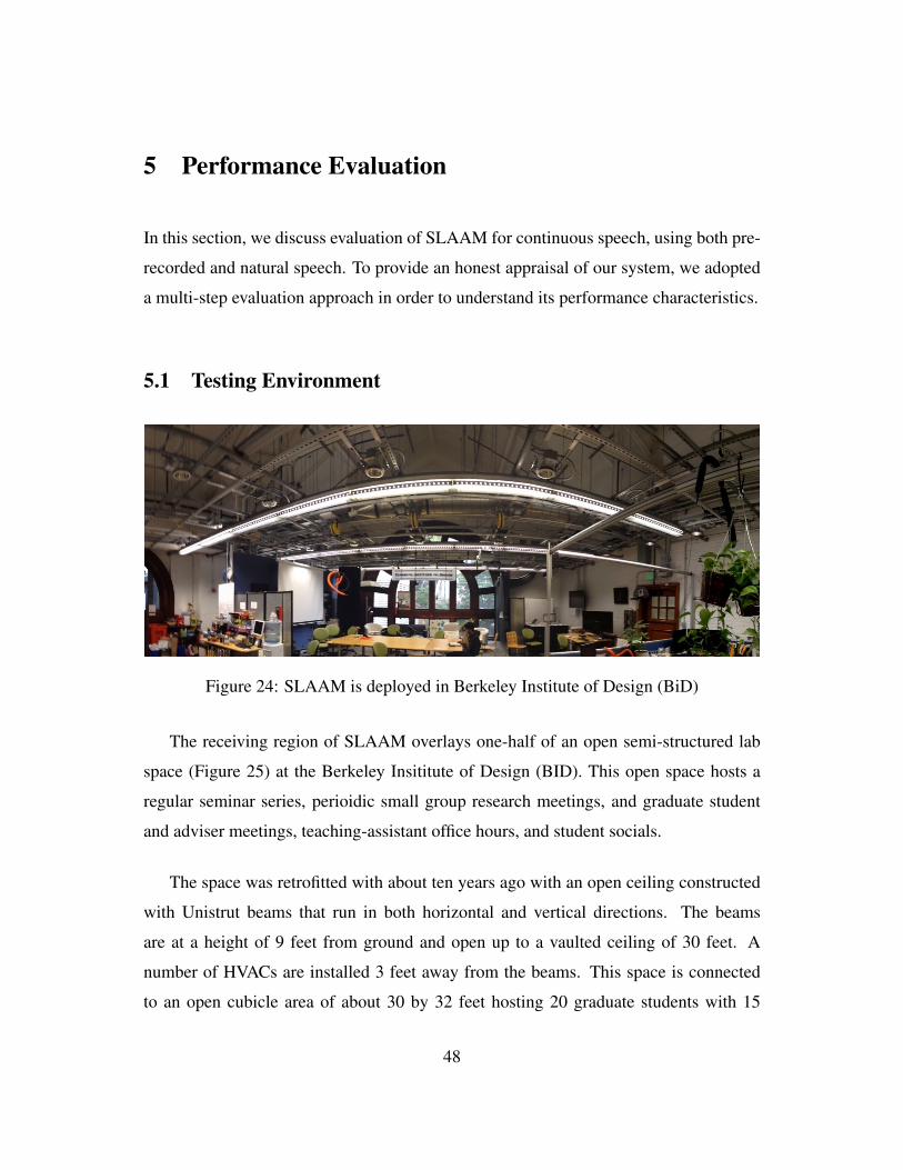
Figure 24: SLAAM is deployed in Berkeley Institute of Design (BiD)
The receiving region of SLAAM overlays one-half of an open semi-structured lab
space (Figure 25) at the Berkeley Insititute of Design (BID). This open space hosts a
regular seminar series, perioidic small group research meetings, and graduate student
and adviser meetings, teaching-assistant office hours, and student socials.
The space was retrofitted with about ten years ago with an open ceiling constructed
with Unistrut beams that run in both horizontal and vertical directions. The beams
are at a height of 9 feet from ground and open up to a vaulted ceiling of 30 feet. A
number of HVACs are installed 3 feet away from the beams. This space is connected
to an open cubicle area of about 30 by 32 feet hosting 20 graduate students with 15
48
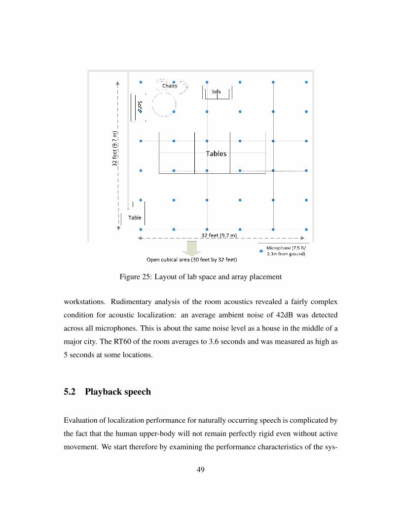
Figure 25: Layout of lab space and array placement
workstations. Rudimentary analysis of the room acoustics revealed a fairly complex
condition for acoustic localization: an average ambient noise of 42dB was detected
across all microphones. This is about the same noise level as a house in the middle of a
major city. The RT60 of the room averages to 3.6 seconds and was measured as high as
5 seconds at some locations.
5.2 Playback speech
Evaluation of localization performance for naturally occurring speech is complicated by
the fact that the human upper-body will not remain perfectly rigid even without active
movement. We start therefore by examining the performance characteristics of the sys-
49
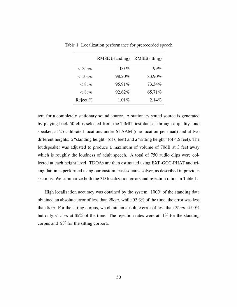
Table 1: Localization performance for prerecorded speech
RMSE (standing) RMSE(sitting)
< 25cm 100 % 99%
< 10cm 98.20% 83.90%
< 8cm 95.91% 73.34%
< 5cm 92.62% 65.71%
Reject % 1.01% 2.14%
tem for a completely stationary sound source. A stationary sound source is generated
by playing back 50 clips selected from the TIMIT test dataset through a quality loud
speaker, at 25 calibrated locations under SLAAM (one location per quad) and at two
different heights: a “standing height” (of 6 feet) and a “sitting height” (of 4.5 feet). The
loudspeaker was adjusted to produce a maximum of volume of 70dB at 3 feet away
which is roughly the loudness of adult speech. A total of 750 audio clips were col-
lected at each height level. TDOAs are then estimated using EXP-GCC-PHAT and tri-
angulation is performed using our custom least-squares solver, as described in previous
sections. We summarize both the 3D localization errors and rejection ratios in Table 1.
High localization accuracy was obtained by the system: 100% of the standing data
obtained an absolute error of less than 25cm, while 92.6% of the time, the error was less
than 5cm. For the sitting corpus, we obtain an absolute error of less than 25cm at 99%
but only < 5cm at 65% of the time. The rejection rates were at 1% for the standing
corpus and 2% for the sitting corpora.
50

5.3 Human speakers
We consider the case of a single, stationary human speaker. For this we recruited seven
subjects and each subject was assigned to 3 different locations under the coverage of
SLAAM. Ground truth was established by calibrating the locations relative to SLAAM’s
geometry via a Berger TLM100 laser range finder. At each location, a subject read aloud
the content of a paper written in English. This was repeated for both standing as well
as sitting heights. We asked the subjects to speak naturally at a normal conversational
volume and pace, and did not ask them to remain consciously rigid during the recording
process. Under each condition, a multichannel track recording of 2.5-3 minutes was
obtained. Localization was performed in real-time on the fly and the location estimates
and residuals were also recorded. This corpus contained an average of 18 minutes of
audio recording for each of the seven subjects.
For each condition, we consider the RMS deviation of the estimated source location
from the calibrated locations. The results are summarized in Table 2. For the stand-
ing corpus, 95.2% of the estimates were less than 10cm of error. No error exceeded
the permissible margin of 25cm. Localization performance is slightly worse for the sit-
ting corpus; the mean deviation from the calibrated locations was 8.8cm and 92.5% of
estimates were below 25cm.
Given the ceiling-mount construction of the array, the distance of a sound source
to the microphones will increase at sitting height. Thus we expect the signal strength
to degrade in proportion to inverse distance squared, which contributes to the increase
in RMSE. Furthermore, some of the error could be attributed to slight movements of a
subject’s upper-body position (e.g. head movement).
51
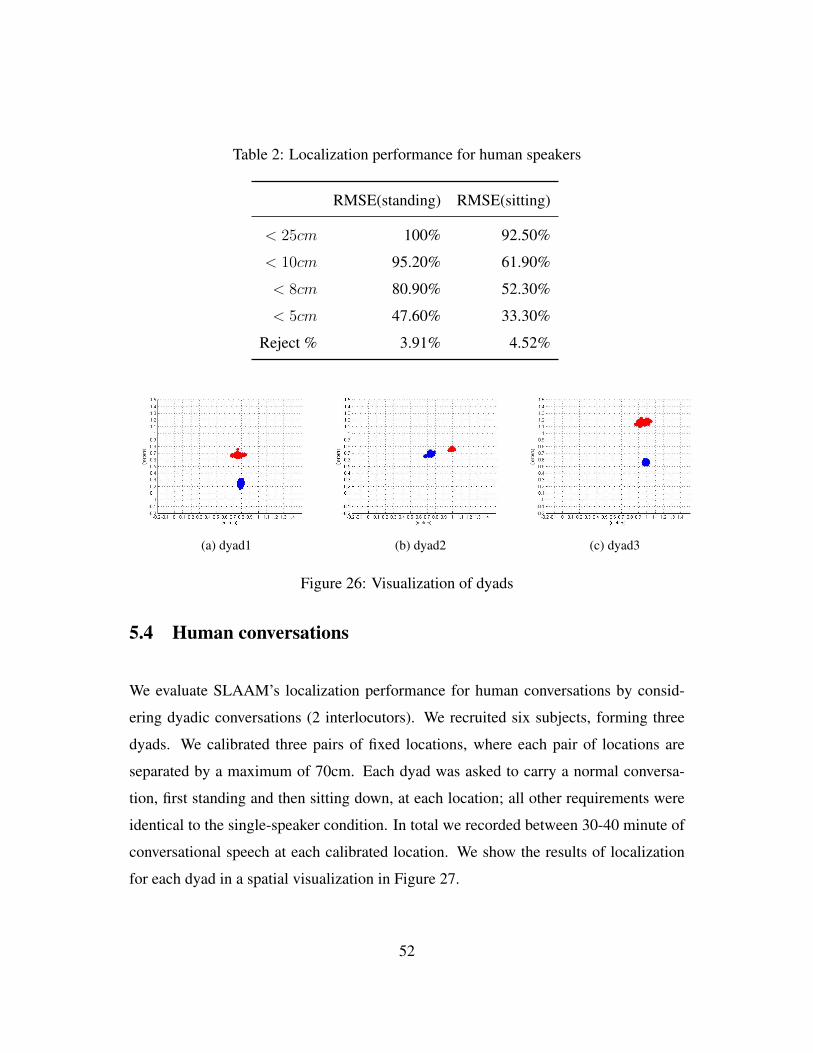
Table 2: Localization performance for human speakers
RMSE(standing) RMSE(sitting)
< 25cm 100% 92.50%
< 10cm 95.20% 61.90%
< 8cm 80.90% 52.30%
< 5cm 47.60% 33.30%
Reject % 3.91% 4.52%
(a) dyad1 (b) dyad2 (c) dyad3
Figure 26: Visualization of dyads
5.4 Human conversations
We evaluate SLAAM’s localization performance for human conversations by consid-
ering dyadic conversations (2 interlocutors). We recruited six subjects, forming three
dyads. We calibrated three pairs of fixed locations, where each pair of locations are
separated by a maximum of 70cm. Each dyad was asked to carry a normal conversa-
tion, first standing and then sitting down, at each location; all other requirements were
identical to the single-speaker condition. In total we recorded between 30-40 minute of
conversational speech at each calibrated location. We show the results of localization
for each dyad in a spatial visualization in Figure 27.
52
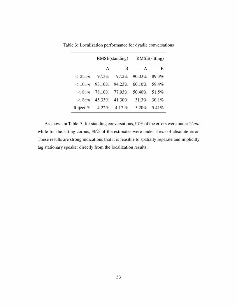
Table 3: Localization performance for dyadic conversations
RMSE(standing) RMSE(sitting)
A B A B
< 25cm 97.3% 97.2% 90.03% 89.3%
< 10cm 93.10% 94.23% 60.10% 59.4%
< 8cm 78.10% 77.93% 50.40% 51.5%
< 5cm 45.33% 41.30% 31.3% 30.1%
Reject % 4.22% 4.17 % 5.20% 5.41%
As shown in Table 3, for standing conversations, 97% of the errors were under 25cm
while for the sitting corpus, 89% of the estimates were under 25cm of absolute error.
These results are strong indications that it is feasible to spatially separate and implicitly
tag stationary speaker directly from the localization results.
53
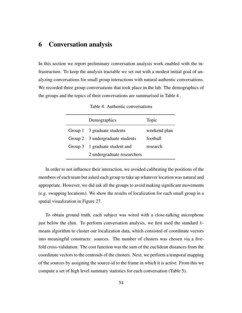
6 Conversation analysis
In this section we report preliminary conversation analysis work enabled with the in-
frastructure. To keep the analysis tractable we set out with a modest initial goal of an-
alyzing conversations for small group interactions with natural authentic conversations.
We recorded three group conversations that took place in the lab. The demographics of
the groups and the topics of their conversations are summarised in Table 4 .
Table 4: Authentic conversations
Demographics Topic
Group 1 3 graduate students weekend plan
Group 2 3 undergraduate students football
Group 3 1 graduate student and research
2 undergraduate researchers
In order to not influence their interaction, we avoided calibrating the positions of the
members of each team but asked each group to take up whatever location was natural and
appropriate. However, we did ask all the groups to avoid making significant movements
(e.g. swapping locations). We show the results of localization for each small group in a
spatial visualization in Figure 27.
To obtain ground truth, each subject was wired with a close-talking microphone
just below the chin. To perform conversation analysis, we first used the standard k-
means algorithm to cluster our localization data, which consisted of coordinate vectors
into meaningful constructs: sources. The number of clusters was chosen via a five-
fold cross-validation. The cost function was the sum of the euclidean distances from the
coordinate vectors to the centroids of the clusters. Next, we perform a temporal mapping
of the sources by assigning the source-id to the frame in which it is active. From this we
compute a set of high level summary statistics for each conversation (Table 5).
54
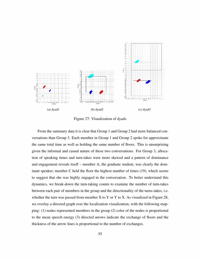
(a) dyad1 (b) dyad2 (c) dyad3
Figure 27: Visualization of dyads
From the summary data it is clear that Group 1 and Group 2 had more balanced con-
versations than Group 3. Each member in Group 1 and Group 2 spoke for approximate
the same total time as well as holding the same number of floors. This is unsurprising
given the informal and casual nature of these two conversations. For Group 3, alloca-
tion of speaking times and turn-takes were more skewed and a pattern of dominance
and engagement reveals itself – member A, the graduate student, was clearly the dom-
inant speaker; member C held the floor the highest number of times (19), which seems
to suggest that she was highly engaged in the conversation. To better understand this
dynamics, we break-down the turn-taking counts to examine the number of turn-takes
between each pair of members in the group and the directionality of the turns-takes, i.e.
whether the turn was passed from member X to Y or Y to X. As visualized in Figure 28,
we overlay a directed graph over the localization visualization, with the following map-
ping: (1) nodes represented members in the group (2) color of the nodes is proportional
to the mean speech energy (3) directed arrows indicate the exchange of floors and the
thickness of the arrow lines is proportional to the number of exchanges.
55
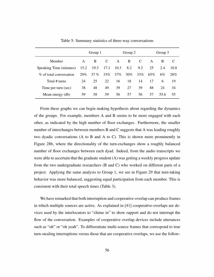
Table 5: Summary statistics of three-way conversations
Group 1 Group 2 Group 3
Member A B C A B C A B C
Speaking Time (minutes) 15.2 19.3 17.1 10.3 8.2 9.2 25 2.4 10.8
% of total conversation 29% 37 % 33% 37% 30% 33% 65% 6% 28%
Total # turns 24 25 22 16 18 14 17 6 19
Time per turn (sec) 38 48 49 39 27 39 88 24 34
Mean energy (db) 59 58 59 56 57 56 57 55.6 55
From these graphs we can begin making hypothesis about regarding the dynamics
of the groups. For example, members A and B seems to be more engaged with each
other, as indicated by the high number of floor exchanges. Furthermore, the smaller
number of interchanges between members B and C suggests that A was leading roughly
two dyadic conversations (A to B and A to C). This is shown more prominently in
Figure 28b, where the directionality of the turn-exchanges show a roughly balanced
number of floor exchanges between each dyad. Indeed, from the audio transcripts we
were able to ascertain that the graduate student (A) was getting a weekly progress update
from the two undergraduate researchers (B and C) who worked on different parts of a
project. Applying the same analysis to Group 1, we see in Figure 29 that turn-taking
behavior was more balanced, suggesting equal participation from each member. This is
consistent with their total speech times (Table 3).
We have remarked that both interruption and cooperative-overlap can produce frames
in which multiple sources are active. As explained in [41] cooperative-overlaps are de-
vices used by the interlocutors to “chime in” to show rapport and do not interrupt the
flow of the conversation. Examples of cooperative overlap devices include utterances
such as “oh” or “oh yeah”. To differentiate multi-source frames that correspond to true
turn-stealing interruptions versus those that are cooperative overlaps, we use the follow-
56
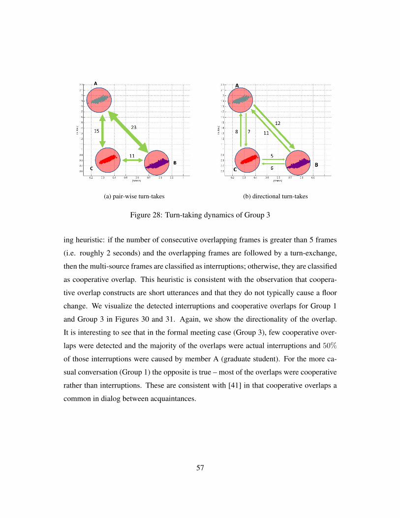
(a) pair-wise turn-takes (b) directional turn-takes
Figure 28: Turn-taking dynamics of Group 3
ing heuristic: if the number of consecutive overlapping frames is greater than 5 frames
(i.e. roughly 2 seconds) and the overlapping frames are followed by a turn-exchange,
then the multi-source frames are classified as interruptions; otherwise, they are classified
as cooperative overlap. This heuristic is consistent with the observation that coopera-
tive overlap constructs are short utterances and that they do not typically cause a floor
change. We visualize the detected interruptions and cooperative overlaps for Group 1
and Group 3 in Figures 30 and 31. Again, we show the directionality of the overlap.
It is interesting to see that in the formal meeting case (Group 3), few cooperative over-
laps were detected and the majority of the overlaps were actual interruptions and 50%
of those interruptions were caused by member A (graduate student). For the more ca-
sual conversation (Group 1) the opposite is true – most of the overlaps were cooperative
rather than interruptions. These are consistent with [41] in that cooperative overlaps a
common in dialog between acquaintances.
57

(a) pair-wise turn-takes (b) directional turn-takes
Figure 29: Turn-taking dynamics of Group 1
(a) Cooperative overlaps (b) Interruptions
Figure 30: Overlapping dynamics of Group 1
58

(a) Cooperative overlaps (b) Interruptions
Figure 31: Overlapping dynamics of Group 3
59
7 Conclusion and Future work
In this work, we have examined the design, implementation, and evaluation of a scalable
microphone array system that is capable of achieving high accuracy, low latency human
speech localization and small-group conversation analysis. We discussed system design
requirements for capturing conversation dynamics, and algorithms and techniques ca-
pable of meeting these requirements. While this work is built on a known localization
strategy using time delays, we achieved significant performance gains over previously
reported results in both precision and recall for localization in a real-world acoustic
environment. Furthermore, we proposed an efficient multi-source localization scheme
under this framework based on peak matching, which was the key enabler to pick up
the nuances in human to human conversations. This working platform has enabled a
number of initial conversation analysis work, revealing interesting patterns of rapport,
interruption, and dominance within different social structures.
There are a number of interesting directions which can be built on this work. We
are currently exploring machine learning techniques, such as Bayesian networks, for
automated analysis and classification of meeting types, speaker roles, and other nuances
of social interaction (e.g. mimicry) on a large scale. We hope that this line of work
will inform models to better understand the formation and evolution of physical social
networks. We have also been exploring uses of this infrastructure for emotion detection,
classification, and feedback for collaborating teams. It is well known that emotional and
social feedback can be powerful incentives to enable teams to function more effectively.
We have since collected a significant amount of authentic conversational and meeting
data for model training and prediction which are being studied. Lastly, microphone
arrays have long been envisioned as ubiquitous input devices and to this end we are
extending the SLAAM API as an array front-end to drive novel speech-based ubicomp
applications.
60
References
[1] G.D. Abowd, A. Battestini, and T. OConnell. The location service: A framework
for handling multiple location sensing technologies. College of Computing and
GVU Center, Georgia Institute for Technology, Atlanta,. Georgia, USA, 2002.
[2] M. Agrawal and K. Konolige. Real-time localization in outdoor environments
using stereo vision and inexpensive gps. In Pattern Recognition, 2006. ICPR 2006.
18th International Conference on, volume 3, pages 1063–1068. IEEE, 2006.
[3] X. Anguera, C. Wooters, and J. Hernando. Acoustic beamforming for speaker
diarization of meetings. Audio, Speech, and Language Processing, IEEE Transac-
tions on, 15(7):2011–2022, 2007.
[4] P.M. Aoki, M.H. Szymanski, L. Plurkowski, J.D. Thornton, A. Woodruff, and
W. Yi. Where’s the party in multi-party?: analyzing the structure of small-group
sociable talk. In Proceedings of the 2006 20th anniversary conference on Com-
puter supported cooperative work, pages 393–402. ACM, 2006.
[5] S. Basu. Conversational scene analysis. PhD thesis, MaSSachuSettS InStitute of
Technology, 2002.
[6] X. Bian, G.D. Abowd, and J.M. Rehg. Using sound source localization in a home
environment. Pervasive Computing, pages 19–36, 2005.
[7] T. Choudhury and A. Pentland. The sociometer: A wearable device for under-
standing human networks. In CSCW’02 Workshop: Ad hoc Communications and
Collaboration in Ubiquitous Computing Environments, 2002.
[8] T. Choudhury and A. Pentland. Sensing and modeling human networks using
the sociometer. In Proceedings of the Seventh IEEE International Symposium on
Wearable Computers (ISWC03), volume 1530, pages 17–00, 2003.
61
[9] P.L. Chu. Superdirective microphone array for a set-top videoconferencing sys-
tem. In Acoustics, Speech, and Signal Processing, 1997. ICASSP-97., 1997 IEEE
International Conference on, volume 1, pages 235–238. IEEE, 1997.
[10] R. Cutler, Y. Rui, A. Gupta, J.J. Cadiz, I. Tashev, L. He, A. Colburn, Z. Zhang,
Z. Liu, and S. Silverberg. Distributed meetings: A meeting capture and broadcast-
ing system. In Proceedings of the tenth ACM international conference on Multi-
media, pages 503–512. ACM, 2002.
[11] E.D. Di Claudio, R. Parisi, and G. Orlandi. Multi-source localization in reverber-
ant environments by root-music and clustering. In Acoustics, Speech, and Signal
Processing, 2000. ICASSP’00. Proceedings. 2000 IEEE International Conference
on, volume 2, pages II921–II924. IEEE, 2000.
[12] J.H. DiBiase. A high-accuracy, low-latency technique for talker localization in
reverberant environments using microphone arrays. PhD thesis, Brown University,
2000.
[13] J.H. DiBiase, H.F. Silverman, and M.S. Brandstein. Robust localization in rever-
berant rooms. Microphone arrays: signal processing techniques and applications,
pages 157–180, 2001.
[14] H. Do, H.F. Silverman, and Y. Yu. A real-time srp-phat source location imple-
mentation using stochastic region contraction (src) on a large-aperture microphone
array. In Acoustics, Speech and Signal Processing, 2007. ICASSP 2007. IEEE
International Conference on, volume 1, pages I–121. IEEE, 2007.
[15] JL Flanagan, DA Berkley, GW Elko, JE West, and MM Sondhi. Autodirective
microphone systems. Acta Acustica united with Acustica, 73(2):58–71, 1991.
[16] JL Flanagan, JD Johnston, R. Zahn, and GW Elko. Computer-steered microphone
arrays for sound transduction in large rooms. The Journal of the Acoustical Society
of America, 78:1508, 1985.
62
[17] D.M. Gavrila. The visual analysis of human movement: A survey* 1. Computer
vision and image understanding, 73(1):82–98, 1999.
[18] Y. Guo and M. Hazas. Localising speech, footsteps and other sounds using
resource-constrained devices. In Proc. of the 10th International Conference on
Information Processing in Sensor Networks, number 2, pages 330–341, 2011.
[19] W. Hahn and S. Tretter. Optimum processing for delay-vector estimation in passive
signal arrays. Information Theory, IEEE Transactions on, 19(5):608–614, 1973.
[20] E.T. Hall. A system for the notation of proxemic behavior1. American anthropol-
ogist, 65(5):1003–1026, 1963.
[21] K. Karahalios and T. Bergstrom. Social mirrors as social signals: Transforming
audio into graphics. IEEE computer graphics and applications, 29(5):22–32, 2009.
[22] D.H. Kim, J. Hightower, R. Govindan, and D. Estrin. Discovering semantically
meaningful places from pervasive rf-beacons. In Proceedings of the 11th interna-
tional conference on Ubiquitous computing, pages 21–30. ACM, 2009.
[23] T. Kim, A. Chang, L. Holland, and A.S. Pentland. Meeting mediator: enhanc-
ing group collaborationusing sociometric feedback. In Proceedings of the 2008
ACM conference on Computer supported cooperative work, pages 457–466. ACM,
2008.
[24] C. Knapp and G. Carter. The generalized correlation method for estimation of time
delay. Acoustics, Speech and Signal Processing, IEEE Transactions on, 24(4):320–
327, 1976.
[25] J. Koo and H. Cha. Autonomous construction of a wifi access point map using
multidimensional scaling. Pervasive Computing, pages 115–132, 2011.
63
[26] R. Kumaresan and D.W. Tufts. Estimating the angles of arrival of multiple plane
waves. Aerospace and Electronic Systems, IEEE Transactions on, (1):134–139,
1983.
[27] D.C. Moore and I.A. McCowan. Microphone array speech recognition: Experi-
ments on overlapping speech in meetings. In Acoustics, Speech, and Signal Pro-
cessing, 2003. Proceedings.(ICASSP’03). 2003 IEEE International Conference on,
volume 5, pages V–497. IEEE, 2003.
[28] F. Nesta and M. Omologo. Generalized state coherence transform for multidi-
mensional localization of multiple sources. In Applications of Signal Processing
to Audio and Acoustics, 2009. WASPAA’09. IEEE Workshop on, pages 237–240.
IEEE, 2009.
[29] A. Pentland and S. Pentland. Honest signals: how they shape our world. The MIT
Press, 2008.
[30] J. Ramırez, J.C. Segura, C. Benıtez, A. De La Torre, and A. Rubio. Efficient
voice activity detection algorithms using long-term speech information. Speech
communication, 42(3):271–287, 2004.
[31] J. Ramırez, J.C. Segura, C. Benıtez, A. de la Torre, and A.J. Rubio. A new
kullback-leibler vad for speech recognition in noise. Signal Processing Letters,
IEEE, 11(2):266–269, 2004.
[32] D. Roy, R. Patel, P. DeCamp, R. Kubat, M. Fleischman, B. Roy, N. Mavridis,
S. Tellex, A. Salata, J. Guinness, et al. The human speechome project. Symbol
Grounding and Beyond, pages 192–196, 2006.
[33] R. Roy and T. Kailath. Esprit-estimation of signal parameters via rotational invari-
ance techniques. Acoustics, Speech and Signal Processing, IEEE Transactions on,
37(7):984–995, 1989.
64
[34] R. Schmidt. Multiple emitter location and signal parameter estimation. Antennas
and Propagation, IEEE Transactions on, 34(3):276–280, 1986.
[35] R.O. Schmidt. A new approach to geometry of range difference location.
Aerospace and Electronic Systems, IEEE Transactions on, (6):821–835, 1972.
[36] J. Scott and B. Dragovic. Audio location: Accurate low-cost location sensing.
Pervasive Computing, pages 307–311, 2005.
[37] H.F. Silverman and S.E. Kirtman. A two-stage algorithm for determining talker
location from linear microphone array data. Computer Speech & Language,
6(2):129–152, 1992.
[38] H.F. Silverman, W.R. Patterson III, and J.L. Flanagan. The huge microphone array.
Concurrency, IEEE, 6(4):36–46, 1998.
[39] J. Smith and J. Abel. Closed-form least-squares source location estimation from
range-difference measurements. Acoustics, Speech and Signal Processing, IEEE
Transactions on, 35(12):1661–1669, 1987.
[40] G. Su and M. Morf. The signal subspace approach for multiple wide-band emit-
ter location. Acoustics, Speech and Signal Processing, IEEE Transactions on,
31(6):1502–1522, 1983.
[41] D. Tannen. Conversational style: Analyzing talk among friends. Oxford University
Press, USA, 1984.
[42] I. Tashev, M. Seltzer, Y.C. Ju, Y.Y. Wang, and A. Acero. Commute ux: Voice
enabled in-car infotainment system. In Mobile HCI, volume 9, 2009.
[43] H. Wang and M. Kaveh. Coherent signal-subspace processing for the detection and
estimation of angles of arrival of multiple wide-band sources. Acoustics, Speech
and Signal Processing, IEEE Transactions on, 33(4):823–831, 1985.
65
[44] M. Wax and T. Kailath. Optimum localization of multiple sources by pas-
sive arrays. Acoustics, Speech and Signal Processing, IEEE Transactions on,
31(5):1210–1217, 1983.
[45] Z. Zhang. Microsoft kinect sensor and its effect. Multimedia, IEEE, 19(2):4–10,
2012.
66
Recommended