2
A METRIC FOR PATTERN-MATCHING APPLICATIONS
TO TRAFFIC MANAGEMENT
Richard Mouncea*
, Garry Hollierb, Mike Smith
c, Victoria J Hodge
b, Tom Jackson
b and
Jim Austinb
a Department of Architecture, University of Cambridge, 1-5 Scroope Terrace, Trumpington Street, Cambridge,
CB2 1PX, UK. Email: [email protected]. Tel: 01223760125. Fax: 01223332960. b Advanced Computer Architecture Group, Department of Computer Science, University of York, York, UK.
Email: [email protected]. c
Department of Mathematics, University of York, Heslington, York, UK. Email: [email protected]. * Corresponding author
Abstract
This paper is concerned with signal plan selection. The paper outlines a system designed to
assist the timely selection of sound congestion-reducing signal control plans; utilising on-line
pattern matching. In this system, historical traffic flow data is continually searched, seeking
traffic flow patterns similar to today’s. If, in one of these previous similar situations, (a) the
signal plan utilised was different to that being utilised today and (b) it appears that the
performance achieved was better than the performance likely to be achieved today, then the
system recommends an appropriate signal plan switch. The heart of the system is “similarity”.
Two time series of traffic flows (arising from two different days) are said to be “similar” if the
distance between them is small; similarity thus depends on the metric or distance between the
two time series. In this paper a simple example is given which suggests that utilising the
standard Euclidean distance between the two sequences comprising cumulatives of traffic flow
may be better than utilising the standard Euclidean distance between the two sequences of
original traffic flow data. The paper also gives measured on-street public transport benefits
which have arisen from using a simple rule-based (responsive) signal plan selection system,
compared with a time-tabled, or fixed-time, signal plan selection system.
Keywords: Pattern matching, Signal plan selection, Cumulatives, Intelligent decision support.
1. Introduction
Travel is fundamental for the social, economic and cultural development of modern society; as
an increasing population seeks ever-increasing mobility. This results in increasing congestion,
especially in cities. How to address growing congestion in cities world-wide has been
recognised as one of the major challenges in the 21st century, especially as currently more than
50% of the world’s population now live in cities.
One of the tools that may be utilised to reduce congestion is the traffic control system. This
paper considers pattern matching as part of an intelligent decision support (IDS) system aimed
at helping to recall traffic signal control plans which worked well in the past (so that these
successful plans may be re-utilised). The paper supposes that a list of signal control plans is
already given and does not consider the generation or design of new signal plans.
1.1. Pattern-matching-based signal control plan selection

3
Given a list of signal control plans, the aim of a pattern-matching-based signal-plan selection
system is (1) to recognise (quickly) those situations occurring today which have arisen
(approximately) in the past, (2) to recall the specific signal plans which worked well in the
past (if any), and (3) of those signal plans recalled, to recommend the most relevant plan
change for implementation now. The central assumption is that
what happens next is (likely to be) what happened before.
The pattern-matching signal control system proposed here was designed in conjunction with
the City of York. The stated aim of the City was to reduce Park and Ride journey times
without significantly damaging car travel times; the policy tool agreed was to switch signal
timing plans suitably. [The list of signal timing plans was here regarded as fixed; although
some very limited signal timing plan “design” was undertaken.]
1.2 A very short technical context
Ritchie (1990) and Zhang and Ritchie (1994) design an integrated set of expert systems to
process real-time data where learning possibilities are envisaged. Hernandez et al. (1999)
introduced the TRYS system for building intelligent traffic management systems. Results of
applying ramp metering strategies have been obtained by Haj-Salem and Papageorgeiou
(1995). A recent review of current techniques for utilising ITS in traffic management is
provided by Papageorgiou et al (2007).
Broadly speaking, the work in this area addresses one or more of the following three
questions.
Question 1 (concerning signal plan selection): for a given scenario, now, how should a signal
plan be selected (from a given list or library of signal plans)?
Question 2 (concerning signal plan design): for a given scenario, how should new signal
timing plans be designed for that scenario?
Question 3 (concerning adaptive or responsive control): how should signals adapt or respond
(automatically) to traffic flows as these change?
The above questions are relevant over different time-scales: signal plan selection and
responsive control should both ideally operate very quickly, while signal plan design must
necessarily be much more laborious and hence slow.
It is natural to utilise pattern matching as an element in seeking to address question 1; and
pattern matching may also have relevance to question 2. Felici et al (2006) seek to address
both questions 1 and 2. Wiering et al (2004) outline a method of using pattern matching to
help find good signal timings. Weijermars (2007) and Thomas et al (2008) present
compendious and interesting analyses of traffic flow variations; various possible applications
(including pattern matching applications) are mentioned but not discussed in any detail. They
identify (a) seasonal variations with time scales of a week or more, (b) periodic variations at
time scales of about 30 minutes and (c) noise. This paper is concerned mainly with question 1,
concerning signal plan selection using pattern matching; but the paper also gives a brief
description of a simple rule-based signal plan selection system together with on-street results
of applying it. The paper makes a few comments on signal plan design and also outlines some
technical data matters concerning the City of York.
There is a vast literature on question 3 concerning responsive signal control. The most well-
known responsive rule for adjusting signal timings is the equisaturation rule devised by
Webster (1958). Such rules, together with many others, are now utilised in the majority of

4
responsive signal control systems operating in the world today; aiming to approximately
optimise signal timings by utilising (reasonably quick) responses to traffic flow changes.
1.2.1 Technical data management and the traffic flow data utilised
The City of York has an Urban Traffic Management and Control (or UTMC) system; this is
designed to have published interfaces so as to aid the utilisation of all information flowing
through the system. Every 5 minutes the UTMC system in York publishes the number of
vehicles which have crossed each detector in the previous 5 minutes; the pattern-matching
system was designed to utilise this “5-minute” traffic flow data.
1.2.2 Signal plan selection using pattern matching
Hauser, Scherer and Smith (2000) consider the opportunities for data mining to help design
switching points in timetabled traffic control systems (the separate traffic control plans are
given and fixed-time). Hegyi et al (2001) suggest using fuzzy logic based traffic control to
manage non-recurrent congestion. De Schutter et al. (2003) extend this, combining case-based
reasoning and fuzzy logic to develop a multi-agent evaluation system that can be used by
traffic operators to analyse the expected performance of several potential (given)
interventions. Zografos et al. (2002) developed an intelligent decision support system to
reduce incident duration by integrating mathematical models, rules and algorithms with
display technologies, allowing faster more accurate interventions. Almejalli et al. (2007)
combine fuzzy logic, a neural network and a genetic algorithm to assist network operators by
estimating the likely effectiveness of (given) interventions. Chen et. al. (2006) outline the
design of a large-scale decision support system for Beijing.
1.2.3 Signal plan design
Kotsialos et al (2002) utilise non-linear optimal control theory to design motorway control
systems; Hegyi (2004) outlines how model predictive control may be used to put together a
coherent package of traffic control measures; van den Berg et al (2008a, b, 2009) and Shu Lin
et al (2010) outline methods for designing interventions using mixed integer linear
programming, within a model predictive control framework. (Thus far their main emphasis has
not been on traffic signal control itself; however there are implications in their work for the
design of traffic signal control plans.) Dealing specifically with traffic signal control in
networks, Angulo et al (2011) suggest ways of optimising (and implementing) signal control
plans using soft computing techniques and Smith (2009, 2010) and Smith and Mounce (2011)
suggest a new way of designing fixed time signal plans suitable for different scenarios, using
models. Smith (2006) applies bilevel optimisation to this problem; it would be interesting to
compare this to approaches based on model predictive control.
1.3 Signal plan selection using rules: a real-life result
Reasonably simple rule-based signal plan selection methods avoid most of the operational
delays which arise with a fully-fledged pattern-matching signal-plan change method; and even
simple rules may yield significant benefits, as is suggested by the results shown here.

5
On the Hull Road in York general traffic is gated every day at one traffic signal by
implementing a small green-time upstream of a bottleneck, moving a queue of general traffic
heading for the City upstream to where the queue may be passed by buses.
The system currently utilised to select the gating plan is a simple time-table plan:
implement gating between 07:45 and 09:15.
In our demonstration this was changed to the following very simple rule-based signal plan
selection system:
when the flow past a specified detector exceeds 68 vehicles in three consecutive 5-minute
intervals then activate gating; and
when the flow past a specified detector is less than 68 vehicles in three consecutive 5-minute
intervals then de-activate gating.
This responsive rule, and the gating strategy itself, were arrived at by model-based
optimisation and some trial and error data modelling; this modelling tested seven different
alternative plan selection rules off-line using flow data from the road network. (See Hodge et
al (2010) for details.) The results obtained are shown in table 1.
Average bus journey time Standard deviation of bus journey time
Timetabled gating 180 seconds 91 seconds
Responsive gating 159 seconds 65 seconds
Table 1: On –street results for a.m. bus journey times with timetabled gating and rule-based,
responsive, gating. Under the timetabled plan selection regime there were 508 journeys and
under the rule-based responsive plan selection regime there were 61.
These results suggest that, compared to time-tabled signal plan selection, a simple responsive
rule-based plan selection is likely to reduce the mean morning bus journey time; and is also
likely to reduce the spread of morning bus journey times, improving bus journey time
reliability.
2 A pattern matching system for signal plan selection
The plan selection system described here requires flows and signal plans to be stored so as to
allow quick recall. An evaluation or performance index must also be calculated and stored.
Pattern matching may then be used to determine a few of the most relevant or close matches
(to today) from the past. The plan switch recommended then depends on (1) the distances to
the matches selected (a small distance means that this past day was very similar and so
relevant to today) and (2) the performance indices (PIs) of the corresponding (flow pattern,
signal plan) pair.
2.1. Examples of performance indices.
There are very many possible performance indices or PIs. The ones we agreed with the City of
York Council, and which led to the results in section 1.3 above, were:
average public transport journey time along the Hull Road and
standard deviation of the public transport journey time along the Hull Road.
Another example of a PI is:
average journey time for cars.
Clearly, there are interactions between the PIs chosen, the interests of the local authority and
the data gathering facilities available. The City of York has a great interest in improving and

6
monitoring bus performance so as to encourage car travellers to park their cars on the outskirts
of York and use Park and Ride buses to reach the historic City.
2.2. Suggested technique for signal plan selection.
The aim is to recover those flow patterns which have the best (smallest) PIs on the days most
similar to today. So suppose that we have found, in the historical record, the k flow patterns
flow pattern 1, flow pattern 2, flow pattern 3, . . . , flow pattern k which are closest to today’s flow pattern so far; that is to flow pattern 0. Suppose that we also
have recovered the corresponding signal plans utilised; let signal plan n be the plan utilised
with flow pattern n. Suppose also given the corresponding performance indices or PIs; with
PI(n) being the PI associated with the (flow pattern n, signal plan n) pair. For 1 ≤ n ≤ k, let
R(n) = [PI(0) – PI(n)]
be the estimated reduction R(n) in the PI which would arise if plan 0 was switched to plan n
and
Q(n) = R(n)/dist[flow pattern n, flow pattern 0].
It would then be reasonable to continually suggest for implementation plan n* where n*
maximises Q(n) (for 1 ≤ n ≤ k), provided Q(n*) exceeds an agreed positive threshold th. (It
would not be good to change plans for diminutive estimated rewards.) R stands for
“reduction” and Q stands for quotient or ratio and estimates the reward / risk ratio, assuming
that reward is proportional to the predicted decrease in the PI and risk is proportional to
dist[flow pattern n, flow pattern 0].
Figure 3 in appendix 1 is designed to be a user-friendly representation of this process; so as to
aid the decision-maker. In figure 3 the estimated reductions in the PI are shown on the vertical
axis and the distance of the historical cases to today’s flow pattern are shown on the horizontal
axis. To change to the plan on day m one would wish to see R(n) large (predicting a large
benefiot from the switch) and a small dist[flow pattern n, flow pattern 0] (giving confidence);
or a large Q(n).
The Intelligent Decision Support system would then continually send simple messages to
transport operators always recommending plan n* where
Q(n*) ≥ Q(n) if 1 ≤ n ≤ k; and also Q(n*) ≥ th > 0. (1)
Plan n* could be automatically implemented if the system had generated sufficient trust and
facilities are available. To build confidence the initial threshold th might be large, to be
reduced over time. There are natural generalisations: it would perhaps be natural to let F be
any convex increasing positive function and to put:
QF(n) = F{[PI(0) – PI(n)]}/dist[(flow pattern n, flow pattern 0)].
The continual recommendations would then still be determined by (1) but with QF instead of
Q. A steep F will recommend few plan changes and if F is the identity then QF(n) = Q(n) and
we have the previous scheme.
To do the selection in a short period of time it is important to be able to search very large
databases very quickly.
2.3 Fast large k-NN searches
Standard k-NN pattern matching is known to be a robust and flexible method that allows the
pattern matcher to be updated continuously. However one drawback is the speed of the
standard method, which typically becomes slow for large problems.

7
An efficient version of k-NN, based on the Advanced Uncertain Reasoning Architecture
(AURA) (Austin et al., 1998; Hodge and Austin, 2005), may be used to overcome this
problem. AURA is a library of methods and applications built on binary neural networks and
designed for high speed search and match operations in large data sets; AURA is thus fast,
scalable and compact. Data may include (1) flow and occupancy data from a number of loop
detectors at signals and elsewhere, (2) travel time data from a number of bus stops or buses,
and (3) other data such as travel times estimated from GPS data.
For each 5-minute period, on each day, the above data may be concatenated into a single
current “5-minute attribute value vector” and then matched against past “5-minute attribute
value vectors”.
Derived data, such as the flow/occupancy ratio (see Han et al., (2009)), may also be utilised.
Further, it is also natural to utilise road works data, special events data, and weather data. The
purpose of using this additional data is to add precision to the matching of past traffic patterns
to today’s patterns. For example it would be natural on a Race Day at York to look only at
previous Race Days when seeking matching traffic patterns from past. Finally it would also be
natural to use data derived from running offline models.
2.2 Flows or cumulative flows?
Pattern matching in this context requires the dis-similarity or distance between two time series.
The Euclidean distance between two such time series
u = {u1, u2, u3, ... un} and v = {v1, v2, v3, ... vn}
(each representing flows in each 5-minute time period stretching between times t1 and tn+1) is
d(u, v) = [(u1- v1)2 + (u2- v2)
2 + (u3- v3)
2 + . . . + (un- vn)
2]
1/2. (2)
When the time series u and v above are time series of flows, with co-ordinates representing the
flows in each 5-minute time period stretching between times t1 and tn+1, there is always the
alternative of using use cumulative flows instead. To do this, we first calculate the
corresponding time series of cumulative flow values
U = { U1, U2, U3, . . . Un} and V = { V1, V2, V3, . . . Vn}
by putting U1 = u1, U2 = u1+ u2, U3 = u1+ u2+ u3, etc. And only then use Euclidean distance.

8
Figure 1. Time series, u, v and w and the corresponding cumulative flow series, U, V and W.
Consider the following three time series comprising 10 consecutive 5-minute flow values:
Time series 1: u = (1, 1, 1, 1, 1, 1, 1, 1, 1, 1), so that U = (1, 2, 3, 4, 5, 6, 7, 8, 9, 10).
Time series 2: v = (0, 2, 0, 2, 0, 2, 0, 2, 0, 2), so that V = (0, 2, 2, 4, 4, 6, 6, 8, 8, 10).
Time series 3: w = (0, 0, 0, 0, 0, 0, 0, 0, 0, 0), so that W = (0, 0, 0, 0, 0, 0, 0, 0, 0, 0).
All six time series are shown in figure 2; u, v, w are the given time series of flows and U, V, W
are the corresponding cumulatives. Using the Euclidean distance formula directly,
d(u,v) = n½ = d(u,w).
On the other hand, using the Euclidean distance on the sequences of cumulative flows:
d(U,V) = [½n]½ and
d(U,W) = [n(n + 1)(2n + 1)/6]½
= [(n + 1)(2n + 1)/3]
½ [½n]
½.
So that, as n = 10,
d(U,W)= [(n + 1)(2n + 1)/3]½d(U,V) = [11.21/3]
1/2d(U, V) = [77]
1/2d(U, V) > 8 d(U, V).
Thus, for n = 10 and for these three time series u, v, and w, the Euclidean distance function
indicates that v and w are equidistant from u. In contrast, Euclidean distance indicates that W is
more than eight times as far away from U as V is. It is then natural to ask: which time series is
more significant or “better” for matching in this traffic flow context? Plainly nearest
neighbours may well vary according to the way the Euclidean metric is utilised.
The original time series of 5-minute flows may be expected to give more information more
quickly when there is a sudden change caused by a sudden serious accident; on the other hand
it may exaggerate traffic impacts when (for example) everything is 5 minutes late. Cumulative
flows may be better at detecting such a 5-minute shift and also may be better at diagnosing
rather more long running and subtle changes brought about on a single day by a “minor”
blockage leading rather gradually to problems, re-routeing caused by a rather distant accident
or minor breakdowns in signal operation. Cumulative flows must also be better at detecting
more long term systematic changes such as an increase in the flow of tourists or the number of
0
1
2
3
4
5
6
7
8
9
10
1 2 3 4 5 6 7 8 9 10
u
U
v
V
w, W
U
u
v
W, w
V

9
school runs at certain times of year. It may be that, for a given input sequence u of five-minute
flows, the “state” of the link flow at a particular time might, for most purposes, be better
measured by the corresponding cumulative flow sequence U.
These considerations give rise to other possible metrics, bearing in mind that 5-minute flows
from a long time past will be irrelevant. (Figure 1 just looks at 10 values; 50 minutes’ worth of
5-minute periods.) So consider sequences of cumulatives over windows of various not-too-
long lengths t (where t is a multiple of l) ending at the current time t0 (also a multiple of l). To
make this precise we choose a not too large number T (T = 10 in the above illustration) and
agree that:
0t now, e.g. 4pm on Thursday 1st October 2011 (t0 is a multiple of l)
l duration of the time period of the data aggregation, e.g. 5 minutes in UTMC,
T duration of the moving time series window stretching backwards from 0t to t0 – T
(all cumulatives utilised lie within this window and T is a multiple of l),
)(ufxflow past location x during time period u stretching from u to (u + l) (where
u is a multiple of l), and
)(0 tFtx , the cumulative flow in the period [t0 – t, t0] is given by:
}),...,(,{ 000
0 )()(
ltlttttu
xtx duuftF
for the values of t = l, 2l, 3l, . . . , T. (each t here is a multiple of l.)
)(0 tFtx is the total or cumulative flow past location x between time tt 0 and time
0t . We then
consider the following sequence of cumulatives over the whole window of duration T:
)(0 lFtx , )2(0 lF
tx , )3(0 lF
tx , . . . , )(0 TF
tx .
Figure 2 illustrates cumulative flows on the moving time series window; clearly T needs to be
carefully calibrated in order to capture the correct time scale for detecting significant events. It
would be natural to have copies of this system with different values of T to capture differing
time-scales of different traffic phenomena. (T = l yields the original distance function (2).)
Let X denote the set of locations x at which detectors are located and let Xx
t
x
tFF )( 00
denote the vector of cumulative flow functions looking backwards from time t0. Then define
the distance between cumulative vector flow profiles 0tF and 1tF as follows:
time
cum
ula
tive
flow
Figure 2. The moving time series window for flow at location x
0tTt 0 tt 0
time series window
)(0 tFt
x
10
x
Tt
lt
t
x
t
x
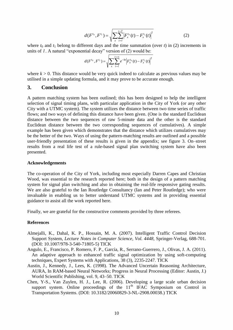
tttFtFFFd
2
)()(),( 1010 (2)
where t0 and t1 belong to different days and the time summation (over t) in (2) increments in
units of l . A natural “exponential decay” version of (2) would be:
x
t
lt
tx
tx
kttttFtFeFFd
2
)()(),( 1010
where k > 0. This distance would be very quick indeed to calculate as previous values may be
utilised in a simple updating formula, and it may prove to be accurate enough.
3. Conclusion
A pattern matching system has been outlined; this has been designed to help the intelligent
selection of signal timing plans, with particular application in the City of York (or any other
City with a UTMC system). The system utilizes the distance between two time series of traffic
flows; and two ways of defining this distance have been given. (One is the standard Euclidean
distance between the two sequences of raw 5-minute data and the other is the standard
Euclidean distance between the two corresponding sequences of cumulatives). A simple
example has been given which demonstrates that the distance which utilizes cumulatives may
be the better of the two. Ways of using the pattern-matching results are outlined and a possible
user-friendly presentation of these results is given in the appendix; see figure 3. On–street
results from a real life test of a rule-based signal plan switching system have also been
presented.
Acknowledgements
The co-operation of the City of York, including most especially Darren Capes and Christian
Wood, was essential to the research reported here; both in the design of a pattern matching
system for signal plan switching and also in obtaining the real-life responsive gating results.
We are also grateful to the Ian Routledge Consultancy (Ian and Peter Routledge); who were
invaluable in enabling us to better understand UTMC systems and in providing essential
guidance to assist all the work reported here.
Finally, we are grateful for the constructive comments provided by three referees.
References
Almejalli, K., Dahal, K. P., Hossain, M. A. (2007). Intelligent Traffic Control Decision
Support System, Lecture Notes in Computer Science, Vol. 4448, Springer-Verlag, 688-701.
(DOI: 10.1007/978-3-540-71805-5) TICK
Angulo, E., Francisco, P. Romero, F. P., García, R., Serrano-Guerrero, J., Olivas, J. A. (2011).
An adaptive approach to enhanced traffic signal optimization by using soft-computing
techniques, Expert Systems with Applications, 38 (3), 2235-2247. TICK
Austin, J., Kennedy, J., Lees, K. (1998). The Advanced Uncertain Reasoning Architecture,
AURA, In RAM-based Neural Networks; Progress in Neural Processing (Editor: Austin, J.)
World Scientific Publishing, vol. 9, 43–50. TICK
Chen, Y-S., Van Zuylen, H. J., Lee, R. (2006). Developing a large scale urban decision
support system. Online proceedings of the 11th
IFAC Symposium on Control in
Transportation Systems. (DOI: 10.3182/20060829-3-NL-2908.00038.) TICK
11
De Schutter, B., Hoogendoorn, S. P., Schuurman, H., Stramigioli, S. (2003). A multi-agent
case-based traffic control scenario evaluation system, Proceedings of the IEEE 6th
International Conference on Intelligent Transportation Systems (ITSC’03), 678-683. TICK
Felici, G., Rinaldi, G., Sforza, A., Truemper, K. (2006). A logic programming based approach
for on-line traffic control, Transport Research Part C, 14 (3), 175-189. TICK
Haj-Salem, H., Papageorgiou, M. (1995). Ramp metering impact on urban corridor traffic:
Field results. Transportation Research Part A, 29(4), 303–319. TICK
Han, J., Krishnan, R., Polak, J. (2009). Traffic state identification using loop detector data.
Proceedings of the International Conference on Models and Technologies for Intelligent
Transportation Systems, Sapienza University of Rome, Italy, (Editor: Gaetano Fusco),
Aracne, 95 - 97. CHECK
Hauser, T., Scherer, W. T., Smith, B. L. (2001) Signal System Data Mining. Research Report
No. UVACTS-15-22-34, Center for Transportation Studies, University of Virginia, USA.
Hegyi, A., De Schutter, B., Hoogendoorn, S., Babuska, R., van Zuylen, H., Schuurman, H.
(2001). A fuzzy decision support system for traffic control centers, Intelligent
Transportation Systems, Proceedings, 2001 IEEE, 358-363.
Zegeye, De Schutter Hellendorn Breunesse XXX
Hegyi, A. (2004). Model Predictive Control for Integrating Traffic Control Measures. Ph.D.
thesis, TRAIL Thesis Series T2004/2, The Netherlands TRAIL Research School.
http://www.hegyi.info/thesis/dep_hegyi_20040203.pdf. TICK when?
Hernandez, J., Cuena, J., Molina, M., (1999) Real-time Traffic Management Through
Knowledge-based Models: The TRYS Approach. In, Tutorial on Intelligent Traffic
Management Models (www.erudit.de), Helsinki, Finland. TICK
Hodge, V.J., Austin, J. (2005). A binary neural k-nearest neighbour technique. Knowledge and
Information Systems, 8(3), Springer-Verlag, 276–292. TICK
Hodge, V.J., Jackson, T., Austin, J. (2010). Optimising Activation of Bus Pre-signals.
Proceedings of the International Conference on Models and Technologies for Intelligent
Transportation Systems, Sapienza University of Roma, Italy, (Editor: Gaetano Fusco),
Aracne, 344 – 353. CHECK
Kotsialos, A., Papageorgiou, M., Mangeas, M., H. Haj-Salem. (2002). Coordinated and
integrated control of motorway networks via non-linear optimal control. Transportation
Research Part C, 10(1), Elsevier, 65–84. TICK
Papageorgiou, M., Ben-Akiva, M., Bottom, J., Bovy, P.H.L., Hoogendoorn, S.P., Hounsell,
N.B., Kotsialos, A., McDonald, M. (2007): ITS and Traffic Management. In
“Transportation” (Handbooks in Operations Research and Management Science Vol. 14),
C. (Editors: Barnhart and G. Laporte) North-Holland (Elsevier), 715-774. XXXX
Ritchie, S. G. (1990). A knowledge-based decision support architecture for advanced traffic
management, Transportation Research Part A: General, 24, 27 - 37. OK
Lin, S., De Schutter, B., Xi, Y., Hellendoorn, H. (2011). Fast Model Predictive Control for
urban traffic networks via MILP. IEEE Transactions on Intelligent Transport Systems, 12
(3), 846 – 856.
Smith, M. J. (2009). A Two-direction Method of Solving Variable Demand Equilibrium
Models with and without Signal Control. Proceedings of the Eighteenth International
Symposium on Transportation and Traffic Theory (Editors: Lam, W. H. K., Wong, S. C.,
Lo, H. K.), Hong Kong, Elsevier, 365 - 386. OK
Smith, M. J. (2010). Intelligent Network Control: Using an Assignment-Control Model to
Design Fixed Time Signal Timings. New Developments in Transport Planning – Advances
in Dynamic Traffic Assignment (Editors: Tampere, C. M. J., Viti, F., Immers, L. H.),
Edward Elgar, 57 – 71. OK
12
Smith, M. J., Mounce, R. (2011). A splitting rate model of traffic re-routeing and traffic
control. Transportation Research Part B, 1389 - 1409. (Also presented at and published in
the Proceedings of the Nineteenth International Symposium on Transportation and Traffic
Theory (Editors: Cassidy, M. J., Skabardonis, A.), Berkeley, Elsevier, 316 – 340.
Smith, M. J. (2006). Bilevel optimisation of prices and signals in Transportation Models. In:
Mathematical and Computational Models for Congestion Charging (Editors:
Lawphongpanich, S., Hearn, D. W., Smith, M. J.), Springer, 159 – 200. OK
Thomas, T., Weijermars, W., van Berkum, E. (2008). Variations in urban traffic volumes.
European Journal of Transport and Infrastructure Research, 8 (3), 251-263. TICK
van den Berg, M., De Schutter, B., Hellendoorn, J., Hegyi, A. (2008a). Influencing route
choice in traffic networks: a model predictive control approach based on mixed-integer
linear programming. Proceedings of the IEEE International Conference on Control
Applications, 299–304. OK
van den Berg, M., Hegyi, A, De Schutter, B., Hellendoorn, J. (2008b). Influencing long-term
route choice by traffic control measures — A model study. Proceedings of the 17th IFAC
World Congress, Seoul, Korea, 13052–13057. OK
van den Berg, M., De Schutter, B., Hegyi, M., Hellendoorn, H. (2009). Day-to-day route
choice control in traffic networks with time-varying demand profiles. Proceedings of the
European Control Conference, Budapest, Hungary, 1776 – 1781. OK
Webster, F. V. (1958), Traffic signal settings, Department of Transport, Road Research
Technical Paper No. 39, HMSO, London. OK
Weijermars, W. (2007). Analysis of urban traffic patterns using clustering, Thesis, University
of Twente, Enschede, Netherlands.
Wiering, M., van Veenen, J., Vreeken, J., Koopman, A. (2004), Intelligent Traffic Light
Control, Technical Report UU-CS-2004-029, Institute of information and computing
sciences, Utrecht University, The Netherlands. OK
Zhang, H., Ritchie, S. G. (1994). Real-Time Decision-Support System for Freeway
Management and Control, Journal of Computing in Civil Engineering, (8), 35-52. OK
(Incidents)
Zografos, K.G., Androutsopoulos, K.N., Vasilakis, G. M. (2002). A real-time decision support
system for roadway network incident response logistics, Transportation Research Part C
(10), 1 - 18. OK
APPENDIX. An intuitive way of representing candidate signal plan changes.
A way of representing the pattern matching results in a compact intuitive way is shown in
figure 3. Five historical (flow pattern, estimated PI reduction) pairs are represented by white
triangles. These are continually plotted (each 5 minutes say) and move against the background
of a fixed cone of acceptable improvement with vertex at the current (flow pattern, 0) pair (the
black triangle). The y-coordinate of triangle 4, for example, gives the estimated reduction in
the PI which would arise if the current plan was changed to that utilized when flow pattern 4
occurred in the past.
The cone of acceptable improvement displays a trade-off between choosing a close match to
the flow today so far (giving confidence, like flow 1 or 2 here which are very like today) and
choosing a plan which gave a small PI in the past, and hence yields a large estimated reduction
in the PI (like the plans associated with flow pattern 4 or 5). The plan associated with flow
pattern 4 looks the best bet here. If the plan corresponding to flow pattern 4 is the same as the
plan corresponding to flow pattern 5 then this diagram would strongly support that plan. Such
perceptions are assisted by the picture shown here in figure 3. Arrows might be added to
indicate the likely direction of movement of each triangle; extrapolated from past results.

13
Figure 3. Five historical (flow, performance reduction) pairs where the flow pattern is close to
today’s flow pattern. The cone of acceptable improvement contains pairs with associated
reasonable signal plans; here only (flow, performance reduction)4 and (flow, performance
reduction)5 have reasonable associated signal control plans.
0 1 2 3 4 5
Distance between (flow)n and (flow)0 for n = 1, 2, 3, 4, 5
R(n)
Estimated
possible
Reductions R(n)
= PI(0) – PI(n)
in today’s
Performance
Index
0
1
2 3
4
5
0
= today’s (flow, estimated performance reduction) pair
= (flow, estimated performance reduction) pairs 1-5 from historical data
Cone of
Acceptable
Improvement
Recommended