1
A new, optimized Doppler optical probe for phase detection, bubble velocity and size measurements:
investigation of a bubble column operated in the heterogeneous regime.
Anthony Lefebvrea*, Yann Mezuib, Martin Obligadob, Stéphane Glucka, Alain Cartellierb
a A2 Photonic Sensors, 38016 Grenoble, France b Univ. Grenoble Alpes, CNRS, Grenoble INP**, LEGI, 38000 Grenoble, France
* Corresponding author: Anthony Lefebvre, [email protected]
** Institute of Engineering Univ. Grenoble Alpes.
Highlights
• A new optical sensor for bubble velocity and size measurements is proposed.
• The sensor gives the bubble translation velocity projected along the fiber axis.
• Reliable data are collected in a bubble column up to 30% global gas holdup.
• A self-similar bubble velocity profile is established in the heterogeneous regime.
• Bubble turbulent vertical intensity reached 55% in the heterogeneous regime.
Keywords
Bubble velocity-size measurements
Local gas flux
Phase detection Doppler optical probe
Dense bubbly flows
Bubble column
Heterogeneous regime
ABSTRACT
A new measuring technique dedicated to bubble velocity and size measurements in complex bubbly flows
such as those occurring in bubble columns is proposed. This sensor combines the phase detection capability of a
conical optical fiber, with velocity measurements from the Doppler signal induced by an interface approaching the
extremity of a single-mode fiber. The analysis of the probe functioning and of its response in controlled situations,
have shown that the Doppler probe provides the translation velocity of bubbles projected along the probe axis. A
reliable signal processing routine has been developed that exploits the Doppler signal arising at the gas-to-liquid
transition: the resulting uncertainty on velocity is at most 14%. Such a Doppler probe provides statistics on
velocity and on size of gas inclusions, as well as local variables including void fraction, gas volumetric flux,
number density and its flux. That sensor has been successfully exploited in an air-tap water bubble column 0.4m
in diameter for global gas hold-up from 2.5 to 30%. In the heterogeneous regime, the transverse profiles of the
mean bubble velocity scaled by the value on the axis happen to be self-similar in the quasi fully developed region
of the column. A fit is proposed for these profiles. In addition, on the axis, the standard deviation of bubble
velocity scaled by the mean velocity increases with Vsg in the homogeneous regime, and it remains stable, close
to 0.55, in the heterogeneous regime.
1. Introduction
Bubble column reactors, where gas is injected at the bottom of an initially stagnant liquid, are widely used in
chemical engineering (e.g. hydrogenation such as in Fischer-Tropsch synthetic fuels production), for bio-chemical
transformations (e.g. in aerobic bioreactors, for algae production…), in waste management (e.g. wet oxidation) or
for flotation units (e.g. deinking of paper, extraction of rare metals…). These reactors are usually operated in the
so-called heterogeneous regime for which the gas concentration typically ranges from 15% to 40%. The resulting
hydrodynamics is complex. A mean large-scale motion takes place in the column consisting of an upward motion
of the liquid with a high gas concentration in the center of the column, compensated by a downward motion of the
liquid with a lower gas concentration near walls. That bubble driven fluid circulation at the reactor scale has been
identified in the sixties, notably by De Nevers, 1968 and by Pavlov and Pozin quoted in Hills, 1974. In addition,
De Nevers, 1968 pointed out that “these circulations are unstable and change size, shape and orientation
chaotically” and that they are the “principal mode of vertical bubble transport”. These unsteady motions arise not
only at the reactor scale but also at smaller length and time scales due to the formation of eddies and of “spiral-
like structures” (e.g. Chen et al., 1994; Ruzicka et al., 2001 and references therein). Owing to such complexity,
and in spite of continuous research efforts since the 60’s, the hydrodynamics of bubble columns still remains
poorly understood. This is manifest from the lack of consensus on scale-up rules for bubble columns as
demonstrated by the number and the variety of correlations that have been proposed so far (e.g. Deckwer, 1992;

2
Joshi et al., 1998; Kantarci et al., 2005; Rollbusch et al., 2015; Kikukawa, 2017; Besagni et al., 2018 to quote a
few).
Similarly, numerical simulations of bubble columns have not yet reached a predictive status since ad-hoc
adjustments are still required notably when the column diameter is varied (e.g. Ekambara et al., 2005). Recently,
the situation regarding scale-up and simulation performances has started to improve thanks to well controlled
experiments performed over an extended range of column diameter (from 0.1 up to 3m) and of gas superficial
velocities, and also with the help of a new measuring technique that provides the Sauter mean diameter of bubbles
evaluated along the horizontal direction (Maximiano Raimundo et al., 2016). Various new features have been
identified from these experiments. The presence of powerful unsteady motions has been confirmed at all column
scales: these motions lead to turbulent intensities about 25-30% on the column axis that grow up to 70% at a radial
distance equal to 0.7 column radius (Maximiano Raimundo et al., 2019). These large fluctuations happen to be a
key characteristic of the heterogeneous regime compared with the homogeneous one, and we tentatively attributed
their origin to the convective instabilities driven by the strong concentration gradients present in these flows.
Indeed, regions with void fraction up to ten times the mean hold-up (denoted as clusters) and down to 0.1 times
the mean hold-up (denoted as voids) have been recently detected in bubble columns operated in the heterogeneous
regime (Maximiano Raimundo, 2015; Maximiano Raimundo et al., 2019). The presence of such concentration
gradients has many consequences. Since these concentration gradients induce buoyancy fluctuations, they are
prone to favor localized shear and hence to drive turbulence production in bubble columns. They are also expected
to enhance the apparent relative velocity between phases as bubbles are preferentially encountered in clusters
while the liquid phase is mostly present in voids. Such an enhancement has indeed been detected in experiments
(see for example Maximiano Raimundo, 2015; Maximiano Raimundo et al., 2019), and it is now accounted for in
simulations (e.g. Maximiano Raimundo, 2015; Gemello et al., 2018) notably by introducing a swarm factor to
correct the drag force such as the one proposed by Simonnet et al., 2007. McLure et al., 2017 have recently
proposed alternate swarm factors that have the peculiarity to depend both on void fraction and on the mean bubble
size. Accounting for such a collective dynamics for bubbles allow two-fluid models to better represent interfacial momentum exchanges. In particular, when including an adapted swarm factor, gas hold-up and liquid velocity on
the column axis agree within ±15% with experiments (Maximiano Raimundo, 2015; Gemello et al., 2018) and
over a significant range of flow conditions (namely for column diameter from 0.12 to 3m and for superficial
velocity from 3 to 35cm/s). Furthermore, that apparent relative velocity has been shown to exceed the terminal
velocity of individual bubbles by a factor up to 3 (Maximiano Raimundo et al., 2019, Maximiano Raimundo,
2015), indicating that the bubble terminal velocity does not control the velocity scale. Instead, the quantity (gD)1/2
has been shown to be a natural velocity scale for the liquid phase in bubble columns and as such, it should appear
in the scale-up rules (Maximiano Raimundo et al., 2019). Such a scale is reminiscent of turbulent flows driven by
convection, a feature that emphasizes further the similarity between confined turbulent convection and bubble
columns in the heterogeneous regime (Maximiano Raimundo et al., 2019).
So far, our understanding of bubble column dynamics relies on local measurements of void fraction, bubble
size and of velocity and Reynolds stress in the liquid phase. Information regarding gas velocity statistics in the
heterogeneous regime is extremely rare. In particular, it is not established whether or not the scale (gD)1/2 also
applies to the gas phase. Fluctuations in the gas velocity that contribute to bubble induced turbulence are not
documented, and, owing to the discussion above, the connection between meso-scale structures and the gas phase
relative velocity needs to be clarified. In that perspective, and as done for turbulent laden flows (Aliseda et al.,
2002; Sumbekova et al., 2016; Huck et al., 2018), measurements of bubble velocities distributions conditioned by
the local void fraction are highly desirable to connect the collective dynamics of bubbles to the characteristics of
cluster and void regions. Clearly, to improve our understanding of momentum exchange mechanisms occurring in
dense bubble columns as well as their representation in two-fluids models, there is a crucial need to gather reliable
statistics on bubble velocities. The present lack of information arises from limitations of available measuring
technique. As imaging or laser based techniques are not suited to investigate dense bubbly flows, previous
attempts have exploited intrusive sensors. Single as well as double optical probes happen to provide erroneous
velocity distributions when used in the heterogeneous regime because of bubbles incoming from the sides of the
probe or from its rear. Indeed, inclined trajectories induce small de-wetting times on mono-fiber probes
(Maximiano Raimundo et al., 2016) and small time of flight between two tips of double (Chaumat et al., 2007) or
of multiple probes (Xue et al., 2003): in all cases, large, unphysical interface velocities are recorded. The above
techniques are therefore too sensitive to the bubble trajectory. Four-tips probes have been designed to better
discriminate between trajectories. Indeed, four-tips probes provide three times-of-flight corresponding to interface
displacements from the central tip to each of the three other tips, and comparing these times-of-flight allows to
recognize and to remove bubble trajectories at an angle with the probe axial direction. Four-tips sensors are
subject to two main limitations. First, they are efficient on bubbles larger than about twice the lateral distance
between probe tips. Efforts have been devoted to diminish that lateral distance down to about 0.5-0.6mm (see Xue
et al., 2003; Mudde and Saito, 2001; Saito and Mudde, 2001; Guet et al., 2003) and even 0.25mm (Sakamoto and
Saito, 2012). The minimum vertical dimension of bubbles properly detected so far with four-tips probes when
used in elementary flows (e.g. isolated bubble, train of bubbles…) is about 1.4 to 1.6mm. In more realistic two-

3
phase flows, when a bubble size below these limits is detected, it is usually discarded from the statistics (Mudde
and Saito, 2001). For actual two-phase flows, a second limitation arises in connection with information
processing. Ideally, identical times-of-flight correspond to bubbles centered on the probe and whose velocity is
directed along the probe axis. Hence, enforcing a strong criterion on the similarity between the time-of-flight
drastically diminishes the fraction of bubbles detected and accounted for in the measurement (Guet et al., 2003):
according to Xue et al., 2003, that decrease can be as large as 99%. In practice, the similarity criterion is relaxed
and its value is selected as a balance between the rise of the data collection rate and the increasing uncertainty.
However, relaxing that criterion leads to some - hard to evaluate - statistical bias as the bubble population is not
uniformly scrutinized. Various improvements have been brought on the signal processing to try to circumvent
these drawbacks. In particular, to properly demodulate the collected information, one has to account for bubble
curvature and shape possibly including oscillations, for its orientation, position and trajectory with respect to the
probe. Consequently, all these variables also contribute to uncertainty sources, and they come in addition to
uncertainties arising from bubble-probe interactions. The later include bubble deceleration, interface deformation
and trajectory distortions notably because of crawling. Harteveld, 2005 carefully investigated uncertainty sources
for four–tip probes and concluded that the mean bubble velocity is usually well captured, but the reliability of gas
velocity fluctuations measurement is far from being ascertained. Owing to the discussion above, it is not
surprising that four-tips sensors have been mostly used in quasi one-dimensional flows where the uncertainty due
to bubble trajectory remains limited. To our knowledge, the only exception is the investigation of churn-turbulent
(i.e. heterogeneous) conditions in a 0.16m I.D. bubble column by Xue et al., 2008. These authors considered a
large range of superficial velocities (from 2 to 60cm/s) leading to local void fractions up to 80%. At a given
position in the column, a four-tip sensor (with a 0.6mm lateral distance between tips) was oriented vertically
upward to gather positive bubble velocities, and then vertically downward to collect negative bubble velocities:
the reconstructed gas velocity distributions exhibited two peaks corresponding to upward and downward motions.
Chord length distributions as well as chord-velocity correlations were also collected. As the distributions included
a zero velocity, Xue et al., 2008 argue that a significant bias may occur in the vicinity of zero velocity as the gas dwell time increases and may become larger than the time scale associated with the change in the flow direction.
Also, part of the uncertainty in velocity measurements was attributed to the oscillations of the interface as large
bubbles, up to a few centimeters in size, were present in the flow. Aside these two comments, the uncertainty was
not quantified, but the authors show that the original results they obtained exhibit consistent trends when varying
the gas superficial velocity. Oddly, Xue et al., 2008 do not provide gas velocity fluctuations or local gas fluxes.
In this context, our objective was to develop a sensor able to provide reliable information on bubble velocities
statistics and on gas flux in the challenging conditions encountered in a bubble column operated in conditions
relevant for industry. The main issue was to ensure a strong sensitivity of the sensor response to bubble trajectory
in order to discriminate meaningful signatures even for distorted gas inclusions experiencing 3D unsteady
motions. To do so, we started from conical optical probes whose reliability in terms of interface detection and
void fraction determination has been proved accurate even in the difficult flow conditions encountered in the
heterogeneous regime (Maximiano Raimundo et al., 2016), and we developed a new sensor that systematically
exploits the Doppler signals collected with a mono-mode optical fiber.
2. Principle of operation, new sensors and their performances on controlled interface
To illustrate the principle of velocity measurements, let us consider an optical fiber with one extremity
immersed in the two-phase flow. Coherent light (frequency f0, wavelength in vacuum 0) is injected in the fiber.
The fraction of incoming light reflected at the immersed tip depends on the refractive index of the media that
surrounds it: this is the principle exploited for phase detection when using optical probes (e.g. Cartellier and
Achard, 1991; Cartellier, 2001). To access the interface velocity V, we considered the Doppler signal formed by
combining the wave reflected at the fiber extremity that has the same frequency as the light source, and the wave
reflected by the approaching interface in the outer medium, that re-enters the fiber and whose frequency has been
Doppler shifted. Let us start with the idealized situation of a plane wave that encounters a reflector approaching at
a velocity V along the direction of propagation of the light beam (Fig.1 with an angle =0). In a fixed frame of
reference, the frequency of the reflected wave equals f0 -2V/ where =0/next is the wavelength in the medium of
propagation those refractive index is next. The beating of the two waves at frequencies f0 and f0 -2V/ provides at
the receiver a signal modulated at the Doppler frequency fD=2V/(0/next). The reflector velocity can thus be
inferred by measuring the Doppler frequency fD. Note that the relevant refractive index next is that of the medium
into which the light propagates. For example, for the front interface of a bubble approaching the sensor, next must
be taken as the refractive index of the liquid. For a probe exiting a gas bubble or for a drop approaching the probe
in a gas, next is the refractive index of the gas. When the velocity of the approaching reflector is at an angle with
the direction of the light propagation, the velocity component to be accounted for is the projection of the interface
displacement velocity (by definition directed along the normal n to the interface) on the direction k of the
incoming wave, i.e. |V n.k| = V cos(). Hence, the Doppler frequency expresses as:

4
(1)
Fig.1: Idealized situation of a planar wave directed along the vector k interacting with a reflector moving at a
speed V along its normal n.
Such a principle has been or exploited a few times in multiphase flows. Using cleaved single mode as well as
multimode optical fibers, Podkorytov et al., 1989 detected Doppler signals due to approaching interfaces during
their investigation of boiling in cryogenic fluids. Doppler signals collected with a multimode optical fiber (50µm
core diameter) were exploited by Sekoguchi et al., 1984 for gas slug velocity measurements in vertical ducts.
Wedin et al. (2000, 2003) used Doppler signatures to access the velocity of O(100) micrometer bubbles with a
single mode fiber (core diameter 9µm): in that case, the measured bubble velocity was corrected for the
deceleration experienced by the gas inclusions when approaching the probe. To investigate surface rheology,
Davoust et al., 2000 exploited Doppler technique on capillary waves. Recently, Chang et al., 2003 measured the
velocity of solid particles (15µm in size) transported in a water jet using a mono-mode fiber (core diameter 8µm).
Later, the same sensor was used on millimeter size bubbles in homogeneous flows up to 10% in void fraction by
Lim et al., 2008 as well as on large (a few millimeters) oil droplets suspended in water by Do et al., 2020.
Although known for a long time, that velocity measuring technique has not become a standard, possibly because
of the high frequencies, typically many MHz, to be processed. Indeed, for a 0=1550nm wavelength, a 10m/s air-
water interface provides a 12.9 MHz Doppler frequency. Let us quote that, in the 80-90’s, sensors of that type
were manufactured by Nihon Kagaku Kogyo Corp. and commercialized by Kanomax Int. Corp. (Sekoguchi et al.,
1984) but these products do not seem to be available any more. Nowadays, high-speed (typ. ≥500MHz) converters
with large storage capability (typ. 1 Giga sample at 8bits) are commonly available (at reasonable prices) and are
well suited for the Doppler technique requirements. Beside, the Doppler technique has not been attempted in
complex bubbly flows such as those encountered in bubble columns operated in the heterogeneous regime where
the turbulent intensity is very large (up to 70%), where bubble trajectories could take any angle with respect to the
vertical, and where the flow shifts between upward to downward directions. To our knowledge, the only exception
is due to Chen et al., 2003 who used the above-mentioned Kanomax product to investigate bubble dynamics in
three bubble columns (0.2, 0.4 and 0.8 m I.D.) up to superficial velocities about 9cm/s i.e. within the beginning of the heterogeneous regime. These authors used a fiber with a cleaved extremity and whose diameter has been
diminished from 5mm down to 350µm. They provide radial profiles of void fraction, mean bubble velocity and
average bubble arrival frequency for a probe directed downward (i.e. facing the mean flow) as well as some data
for a probe directed upward. Although they also provide a few bubble velocity distributions, the authors do not
explain how they processed the raw signals, they do not discuss sensitivity to processing nor sensor performances
and they do not explain how they built the distributions from the two data series collected with an upward and
with a downward oriented probe.
2.1 New sensor design
We therefore revisited that technique with the objective of producing reliable data on bubble velocities in
challenging flow conditions. Our bet was that the conditions for collecting the light reflected by an interface back
into an optical fiber should be stringent enough to provide a way to discriminate between bubble trajectories.
Moreover, we introduced an extra novelty on the sensor design to solve another issue. Indeed, all previous
attempts to exploit the Doppler technique were made using cleaved tips normal to the fiber axis. Optical fibers
having significant outer diameters (typically 100µm), such cleaved extremities are far from being satisfactory with
respect to phase detection because of significant disturbances appearing on raw signals (Cartellier, 1990). Since
our goal was to simultaneously access to the phase indicator function and to measure the velocity of bubbles, the
probe tips need to be sharpened to improve the reliability of gas dwell time determination (see the discussion in
Vejrazka et al., 2010). The challenge was therefore to manufacture sharp probes that provide a good contrast
between water and air, and also that are able to detect Doppler signals of large enough amplitude. That objective
is not straightforward. Indeed, the Doppler amplitude is maximized for cleaved tips and it is expected to become
weaker when sharpening the probe tip. Meanwhile, good contrasts between air and water responses are observed
for sharpened tips (Frijlink, 1987; Cartellier and Barrau, 1998a) that are also well adapted for a smooth piercing of
fD
= 2V | n·k |
l0
/ next
Moving reflector
V n
Incoming plane
wave (frequency fo)
Medium of
refractive
index next
Fixed source
and observer

5
incoming interfaces. A balance within these opposite constraints was finally reached by adjusting the curvature at
the very end of conical tips (Fig.2). By fine-tuning that curvature, sharpened tips could be made as reflective as
cleaved fibers, thus granting an optimum design.
Fig.2: a) Example of a conical tip manufactured from a single mode optical fiber - the two images correspond
to the same probe at different magnifications. b) Light intensity distributions measured at various distances from
the fiber extremity and determination of the numerical aperture for cleaved (0C) and conical (1C) extremities. c)
Measured de-wetting time Tm versus the interface velocity V for the conical probe: the latency length as defined
between thresholds at 10% and at 90% of the full signal amplitude is LS = Tm V ≈ 6µm. That relationship is
represented by the dotted line.
The prototypes exemplified Fig.2 were manufactured by A2 Photonic Sensors using a patented technology.
Corning® SMF28 single mode fibers with a 8.2µm core diameter surrounded by a 125µm cladding were used.
These fibers exhibit a neff=1.47 effective group index of refraction at the operating wavelength. The optical fiber
was fed via an optical circulator by a 0=1550nm laser light emitted by a 10mW distributed feedback (DFB) laser:
the narrow spectral width of this device guarantees a coherence length over 5mm. The circulator output was
connected to a photodetector with a 250MHz bandwidth. The optical fiber was glued into a stainless steel tube
0.9mm external diameter and 30mm long: the fiber extremity was located 7mm away from the end of the metallic
tube to minimize the perturbation induced in the flow. The raw signals were digitized by a 12 bits analog-to-
digital converter (ADC) before further signal processing. In order to accurately sample the high frequency
Doppler bursts, the ADC must have both a high acquisition frequency (typically tens of MHz) and a large enough
memory. Fig.3 provides a typical signal collected in an air-water bubbly flow with the prototype Doppler probe
shown Fig.2. The signal exhibits both a clear contrast between water (≈20mV) and air (≈0.45V) and a limited
noise (≈10mV in amplitude) so that the events corresponding to bubble entry and to bubble exit can be easily
identified. In addition, the signal exhibits Doppler oscillations of significant amplitude both at gas-liquid and at
liquid-gas transitions. The amplitude of these Doppler oscillations is significantly larger at the gas-liquid
transition (from 50 to 300mV) than at the liquid-gas transition (from 20 to 90mV). That feature is due to the magnitude of the Fresnel coefficient R12 that provides the reflected intensity with respect to the incoming intensity
I0: one has R1/2=[(n1-n2)/(n1+n2)]2 under normal incidence at the boundary between two media of refractive indices
n1 and n2. The reflection coefficient at the fiber tip /external medium interface amounts to 3.6% in air and to
0.25% in water. The strong contrast between these two values (by a factor larger than 10) forms the basis of the
phase detection capability of optical probes. Concerning the Doppler amplitude, it is related to the intensity
(I1I2)1/2 of the coherent beating between the two returning waves, where I1 denotes the light intensity reflected at
the fiber tip (i.e. I1=Rfiber/ext I0, I0 is the light intensity injected in the fiber) and I2 the light intensity returning in the
fiber after reflection on the moving interface. The latter wave experiences a transmission from the fiber into the
external medium, (the latter is named here medium ext1, and the transmission coefficient is 1-Rfiber/ext1), a
reflection at the moving interface hat separates media a1 and 2 (the coefficient is Rext1/ext2 for a specular reflection)
and a back transmission from the external medium 1 into the fiber (the transmission coefficient is 1-Rfiber/ext1), so
that the returning intensity is given by I2/I0=Rext1/ext2 (1-Rfiber/ext1)2. Hence, I2/I0 has nearly the same magnitude
whatever the external medium since the transmission coefficients are almost the same for air and for water.
Consequently, the Doppler amplitude, that is proportional to [Rfiber/ext Rext1/ext2]1/2 (1-Rfiber/ext1) I0, is controlled by
the intensity reflected at the fiber tip I1 that is by the reflection coefficient Rfiber/ext1. That feature explains why the
amplitudes of Doppler signals are larger when the probe is in air than when it is in water. For the example of
Fig.3, the ratio between the maximum Doppler amplitudes recorded at the gas-liquid transition and at the liquid-
gas transition respectively is about 3.4 which is close to the expected value i.e. (Rfiber/air
/Rfiber/water)1/2=(3.6/0.25)1/2≈3.8. This good agreement holds for an interface very close to the fiber, a position that
maximizes the Doppler amplitude.
6
At larger distances, the spatial distribution of the illumination intensity (see Fig.4 below and the associated
discussion) as well as light collection conditions must be accounted for. They both induce a decrease in the
Doppler amplitude as the distance to the fiber increases, as exemplified Fig.3. Clearly, the Doppler signals extend
much further ahead of the phase transition from air to water than from water to air: for a fixed Doppler amplitude
about 40mV, the former extends up to 33µm while the latter extends only up to 10µm. That feature is directly
connected to the magnitude of the reflection coefficient discussed above, and it is thus quite general. Globally,
Doppler signals with the largest amplitude are collected either when the probe exits a gas bubble or when the
probe enters a drop. These two situations also correspond to longer Doppler signals.
Going back to the example of Fig.3, eq.(1) holds for both Doppler signals so that two velocities can be
estimated for the same bubble. The Doppler frequency before the liquid-gas transition is about 500kHz and it
corresponds to 29cm/s. At the gas-liquid transition, the Doppler frequency is about 330kHz and it provides a
velocity about 26cm/s. These velocity estimates are consistent within 10%. In this example, the second transition
(i.e. from gas to liquid) corresponds to a probe leaving the bubble: it provides a slightly smaller velocity compared
with the bubble entry (i.e. from liquid to gas) because of the bubble deceleration induced by the probe-bubble
interaction as discussed and quantified in Vejrazka et al., 2010. The impact of the deceleration on the reliability of
velocity measurements will be quantified in the next section.
Fig.3: Typical signal from a bubble recorded with the prototype conical single mode optical probe in the
bubble column described in section 3. A low voltage (here ≈ 20mV) corresponds to a probe tip in water while a
high voltage (here ≈ 0.45 Volts) corresponds to a probe tip in gas. The characteristics events, i.e. arrival time tA,
exit time tE and the gas residence time TG are indicated on the crenel-like signal. Doppler signals collected before
the probe hits the bubble (signal to the left) and when the probe leaves the bubble (signal to the right) are
magnified for clarity.
We therefore succeeded to design a new sensor that provides information on the velocity of the approaching
interface and that also ensures efficient phase detection. In particular, its latency length Ls (see Cartellier, 1990) that quantifies the sensor resolution on the interface position determination happens to be quite small, close to
6µm (Fig.2c). Such a resolution is significantly better than that of classical multimode optical fibers for which the
latency length is typically in the range 30 to 60µm. Beside, no sensor calibration is required: once the light
wavelength in the propagation medium is known, the velocity is uniquely determined by the Doppler frequency
using Eq.(1). A last advantage of the technique is the good reproducibility of the manufacturing process. Let us
now examine in more detail the performances of that new sensor called Doppler probe in the sequel.
2.2 Conditions for collecting a Doppler signal and consequences on the nature of the detected velocity
As various velocities are associated with an inclusion and its interface, it is important, as we did for Laser
Doppler Velocimetry (LDV in short) applied to large inclusions (Cartellier and Achard, 1985), to determine the
nature of the velocity detected with the sensor developed here. Let us first underline that eq.(1) involves the
interface displacement velocity that is, by nature, directed along the normal to the interface. This argument holds
for clean interfaces that provide specular diffusion. If solid particles are attached to the interface, and if the light
diffusion by these particles is intense enough to compete with specular diffusion, then the probe may also become
sensitive to the velocity component of the particles tangent to the interface. Such a situation was never
encountered in all the experiments we performed using unfiltered tap water, and, in the following, we do not
consider nor discuss the potential impact of solid particles on the interface.
To identify the nature of the measured velocity, one should account for the conditions required for collecting a
Doppler signal. The latter consists into two main constraints: first, the incoming interface must be located within

7
the zone illuminated by the fiber, and second, the incoming interface must be oriented in such a way that the light
reflected at the moving interface enters back the fiber.
2.2.1 Illuminated zone ahead of the sensor. That zone is partly controlled by the numerical aperture () of
the optical fiber. NA provides the illumination angle with respect to the optical axis in an external medium of
refractive index next according to next sin() = . The numerical aperture depends on the fiber design but it also
changes with the shape of the tip: in particular, the increases for sharp tips compared with cleaved extremities.
The numerical apertures were directly measured from intensity maps (Fig.2-b) recorded in air at various distances
from the fiber exit. At each distance, a Gaussian normalized by the maximum in intensity at that distance was
fitted, and its full-width at a given intensity threshold was plotted versus the distance to the probe to give access to
the numerical aperture: this process is illustrated Fig.2-b for cleaved and for conical tips. The corresponding
numerical apertures are given in Table 1 for various thresholds in intensity. For the cleaved fiber, NA defined for
a 1% threshold (a 1% threshold corresponds to a width of 3 standard-deviations on a Gaussian intensity
distribution) is about 0.12, which is close to the manufacturer value (0.14). For the conical tip, NA is larger: it
ranges from 0.32 when defined at threshold in intensity (the latter corresponds to a width about 2 standard-
deviations on a Gaussian intensity distribution), up to 0.45 for an intensity threshold set at 1%. For NA=0.45, the
emission angle equals 27° in air and 20° in water.
Cleaved fiber Sharpened tip Sharpened tip
(measured at 1%) (measured at 1/e2) (measured at 1%)
NA=0.12 NA = 0.32 NA = 0.45
in air 8° 19°
in water 6°
Table 1: Measured numerical apertures and corresponding illumination angles in air and in water.
These emission angles provide a rough estimate of the lateral limits of the illumination area at short distances
from the fiber tip. Extra conditions must be taken into consideration to identify the active zone of the sensor.
Indeed, along the axial direction, the light coming out of the fiber can be considered as a spherical wave, and its
intensity strongly decreases with the distance r to the fiber extremity. Thus, any absolute detection threshold,
either set by the detector characteristics or by an user-defined value, will control the maximum working distance
of the probe. To evaluate that distance, the light intensity emitted out of a conical fiber tip has been simulated as a
Gaussian beam with a numerical aperture given by the measured NA (consequently, the waist dimension is fixed
for a given wavelength). Iso-intensity contours normalized by the maximum intensity at the waist I0 are mapped in
Fig.4. Strictly speaking, the results shown Fig.4 do not correspond to the actual Doppler amplitude: they account
for the decay of the incoming intensity with the distance from the probe tip but they do not account for reflection
and/or transmission coefficients, and they do not account for the necessary conditions for collecting some light
back into the fiber. However, they remain meaningful for the present discussion because the Doppler amplitude
remains proportional to the incoming intensity plotted in Fig.4. For an absolute incoming intensity equal to 1% of
I0, the axial extent of the probe volume in air is about 42-43µm along the optical axis. The radial extend of that
zone is maximum at a distance r ≈ 25µm and it equals 6-7µm. Hence, the effective illumination angle eff as
defined for an absolute intensity threshold of 1% of I0 is at most about 15° in air (Fig.4 top): it is therefore
significantly smaller than the illumination angle deduced from the numerical aperture (see last column in Table
1). That drastic diminution of the numerical aperture is mainly due to the strong decrease of light intensity with
the distance to the probe. This result also indicates that the effective illumination angle eff can be controlled
through signal processing by setting a minimum on the Doppler amplitude. For a probe tip immersed in water (Fig.4 bottom), an intensity equal to 1% of I0 is reached at a 80µm distance along the axis, and at a maximum
lateral extent about 7-8µm at a 45µm distance: the corresponding effective illumination angle in water happens to
be eff ≈10°, which is slightly less than in air for the same intensity threshold.
To consolidate the above analysis based on Gaussian optics, we measured the probe working distance by
collecting raw signals from planar air-water interfaces obtained by filling or emptying a large (5cm I.D.)
cylindrical tube. For these tests, the conical probe was centered in the tube, its optical axis was perpendicular to
the incoming interface, and the interface motion was controlled and steady (i.e. at constant speed). To compare the
signals collected at various interface velocities, the time scale was transformed into the distance r between the
interface and the probe extremity using the speed of the interface as measured by the Doppler technique. The raw
signals delivered by a 1C probe operated at constant source intensity and fixed detector gain, are shown Fig.5 for
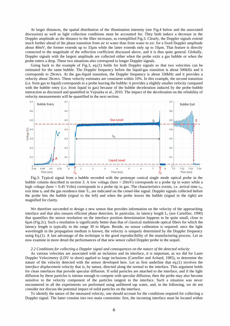
two interface velocities, namely 1cm/s and 59cm/s. On both signals, the working distances in air and along the
optical axis are about 30µm for a threshold set at 5% of the maximum Doppler amplitude. Such distances are
comparable to the ≈19µm value predicted from the emitted light intensity distributions shown Fig.4. These
working distances depend on the Doppler amplitude only: they do not vary with the interface velocity. Moreover,
they are not limited by light coherency since the coherence length of the diode (about 5mm) is always much larger
8
than the optical path. Let us also point out that, for an interface travelling over a distance L, the number of
successive Doppler periods equals 2 next L/0. This is indeed observed in Figure 5, where 26 periods are recorded
over a 20µm distance in air. In water, the number of periods would have been 34.
Fig.4: Light intensity I coming out of the conical fiber tip in air (a) and in water (b) normalized by the
maximum light intensity at the waist I0. The color represents log10(I/I0). Iso-value contours (solid lines) are
provided for I/I0 =10-1, 10-2 and 10-3. The number of fringes corresponds to the number of Doppler periods that
would be collected for an interface travelling from the current location to the probe tip localized at the origin.
Fig.5: Signals collected from a planar air-water interface approaching a conical probe at constant speed (case
a: 1cm/s; case b: 59cm/s) plotted versus the distance between the interface and the probe tip. The transition is
from air to water, and the interface displacement velocity is directed along the fiber optical axis.
It is worth at this stage to compare the responses of cleaved (0C) and of conical (1C) tips. Typical signals are
presented Figure 6: these signals have been simultaneously acquired from 0C and 1C probes located side-by-side
and facing the same planar interface. The optical axes of both probes were normal to the interface. In addition,
comparable source intensity and detector gain were used on the two probes. Clearly, the cleaved probe has a much
longer working distance than the conical probe as it is indeed able to detect Doppler signals up to a millimeter
ahead of its tip compared with 50-100µm for the conical probe. This is because the smaller numerical aperture of
the cleaved fiber induces a smaller decay rate of the incoming intensity with the distance to the probe. This is also
a)
b)
9
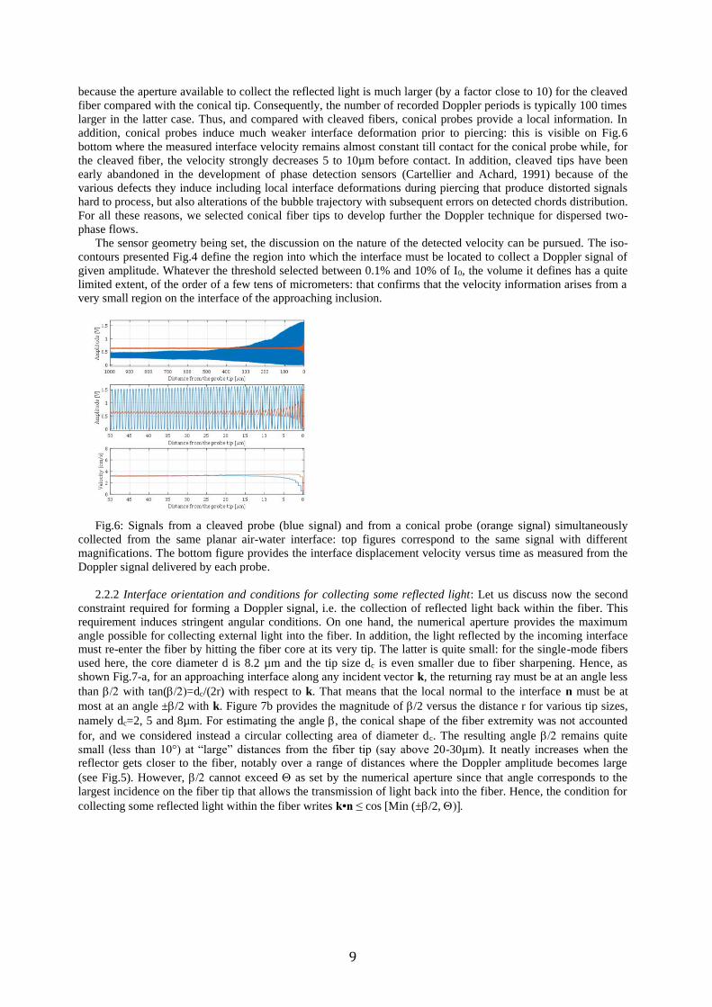
because the aperture available to collect the reflected light is much larger (by a factor close to 10) for the cleaved
fiber compared with the conical tip. Consequently, the number of recorded Doppler periods is typically 100 times
larger in the latter case. Thus, and compared with cleaved fibers, conical probes provide a local information. In
addition, conical probes induce much weaker interface deformation prior to piercing: this is visible on Fig.6
bottom where the measured interface velocity remains almost constant till contact for the conical probe while, for
the cleaved fiber, the velocity strongly decreases 5 to 10µm before contact. In addition, cleaved tips have been
early abandoned in the development of phase detection sensors (Cartellier and Achard, 1991) because of the
various defects they induce including local interface deformations during piercing that produce distorted signals
hard to process, but also alterations of the bubble trajectory with subsequent errors on detected chords distribution.
For all these reasons, we selected conical fiber tips to develop further the Doppler technique for dispersed two-
phase flows.
The sensor geometry being set, the discussion on the nature of the detected velocity can be pursued. The iso-
contours presented Fig.4 define the region into which the interface must be located to collect a Doppler signal of
given amplitude. Whatever the threshold selected between 0.1% and 10% of I0, the volume it defines has a quite
limited extent, of the order of a few tens of micrometers: that confirms that the velocity information arises from a
very small region on the interface of the approaching inclusion.
Fig.6: Signals from a cleaved probe (blue signal) and from a conical probe (orange signal) simultaneously
collected from the same planar air-water interface: top figures correspond to the same signal with different
magnifications. The bottom figure provides the interface displacement velocity versus time as measured from the
Doppler signal delivered by each probe.
2.2.2 Interface orientation and conditions for collecting some reflected light: Let us discuss now the second
constraint required for forming a Doppler signal, i.e. the collection of reflected light back within the fiber. This
requirement induces stringent angular conditions. On one hand, the numerical aperture provides the maximum
angle possible for collecting external light into the fiber. In addition, the light reflected by the incoming interface must re-enter the fiber by hitting the fiber core at its very tip. The latter is quite small: for the single-mode fibers
used here, the core diameter d is 8.2 µm and the tip size dc is even smaller due to fiber sharpening. Hence, as
shown Fig.7-a, for an approaching interface along any incident vector k, the returning ray must be at an angle less
than with tan()=dc/(2r) with respect to k. That means that the local normal to the interface n must be at
most at an angle ±/2 with k. Figure 7b provides the magnitude of /2 versus the distance r for various tip sizes,
namely dc=2, 5 and 8µm. For estimating the angle , the conical shape of the fiber extremity was not accounted
for, and we considered instead a circular collecting area of diameter dc. The resulting angle remains quite
small (less than 10°) at “large” distances from the fiber tip (say above 20-30µm). It neatly increases when the reflector gets closer to the fiber, notably over a range of distances where the Doppler amplitude becomes large
(see Fig.5). However, cannot exceed as set by the numerical aperture since that angle corresponds to the
largest incidence on the fiber tip that allows the transmission of light back into the fiber. Hence, the condition for
collecting some reflected light within the fiber writes k•n ≤ cos [Min (±/2, )

10
Fig.7: a) Schematized emission from the extremity of an optical fiber and angular conditions for detecting an
approaching interface. b) Maximum collection angle /2 allowed for forming a Doppler signal as a function of the
distance r for various diameters dc of the probe extremity (the latter is approximated as a flat circular area).
The above reasoning is strictly valid for a vector k directed along the optical axis (i.e. =0). For a wave vector
at an angle with the optical axis (with in the interval ± ), the incidence of the returning wave on the fiber tip
must be within the collection angle that leads to the condition ±/2 less than Therefore, as increases, the
range of angles leading to a Doppler signal narrows, and in the limit =, the only active ray left corresponds to
the incident vector k. Overall, for Doppler signals to appear, the maximum inclination of the normal n to the
incoming interface with the optical axis should be ±. This result and the above discussion have two
consequences:
- first, the maximum inclination of the interface displacement velocity with respect to the active wave
vector is ± Therefore, a first source of uncertainty on the quantification of the displacement velocity arises
because of the range of eligible interface inclinations for a fixed vector k. In other words, the angle between n and
k involved in eq.(1) varies from 0 to , so that the corresponding uncertainty on the velocity magnitude amounts
for cos() at most. Note that this is a somewhat conservative estimate as the range of angles could be
significantly less than for very thin tips (i.e. small dc) as shown Fig.7-b.
- second, the active vector k can vary when the interface approaches the fiber tip, and one has to account for
such a change during the formation of a Doppler signal. To discuss this aspect, let us introduce the interface
displacement velocity projected along the optical axis, noted Vaxis. According to the above discussion, the velocity
detected using eq.(1) can evolve between Vaxis (for an active wave vector such that =0) and Vaxis cos()
cos(−/2) or Vaxis cos() cos(+/2) when changing the wave vector within acceptable limits. Taking the latter as
± and since the condition ±/2< always holds, the maximum deviation from Vaxis is therefore Vaxis cos2().
A more realistic estimate would consider that the acceptable limits for the inclination of the wave vector
correspond to the effective illumination angle eff introduced above, in which case the maximum deviation from
Vaxis amounts to Vaxis cos() cos(eff).
Overall, the viewing angle (possibly combined with its effective value) controls the uncertainty on velocity
when the latter is interpreted in terms of the interface displacement velocity projected along the probe optical axis.
Fig.8 provides the magnitude of that uncertainty versus the numerical aperture, either using the conservative
estimate cos2(), or using the more realistic estimate cos() cos(eff). According to Fig.8, the uncertainty on
velocity increases with the numerical aperture. In term of sensor optimization, cleaved fibers provide small
apertures (Table 1) but, and as already argued, such geometries are not suited for phase detection. Instead, conical
tips should be preferred. For the conical sensors we manufactured, NA ranges from 0.32 to 0.45 (depending on the
threshold considered, see Table 1), and thus the typical uncertainties range from 10 to 20% in air, and from 6 to
12% in water. Using the more realistic estimate related with the effective aperture eff based on the 10-2 iso-
intensity contour, these uncertainties evolve from 8.4% to 13.7% in air and from 4.3% to 7.2% in water. Overall,
the uncertainties are less than ≈14% for a probe in air, and less than ≈7% for a probe in water: they are thus
acceptable. It is worth underlining that the effective angle, and thus the uncertainty, could be further reduced by
selecting Doppler signals of larger amplitude, but possibly at the price of lower data rates.
According to the conditions required for collecting a Doppler signal, it happens that the proposed sensor
provides the interface displacement velocity projected along the probe optical axis. In addition, the smaller the
numerical aperture, the smaller the uncertainty on the measured velocity magnitude.
a) b)

11
Fig.8: Maximum uncertainty (in percent) on the magnitude of the interface displacement velocity projected
along the probe axis as a function of the numerical aperture for a probe in air (open symbols) or in water (closed
symbols). Results are provided both for the nominal and for the effective numerical aperture.
The companion question to be considered now is to connect the information on the interface displacement
velocity with the translation velocity of the inclusion, a key variable for flow analysis and modeling. We have
seen that the volume probed by that technique is quite small – typically O(10µm) so that only a very limited
portion of the interface of incoming inclusions is scanned by the technique. We have also seen that, to observe
Doppler signals, the normal of incoming interface must make an angle within ±Min( eff) with the probe optical
axis, where eff depends on the selected amplitude threshold on Doppler signals. For an air-water interface, and
for a threshold 10-2 I0, eff has been shown to be about 15° in air and 10° in water. Consequently, the velocity
information always arises from the close vicinity of the apex of the front (or rear) interface of bubbles. For
spheres, for ellipsoids as well as for distorted, wobbling bubbles (Clift et al., 1978), the interface velocity in these
zones is very close to the translation velocity of the inclusion: the difference is driven by the cosine of the angle
and it is less than 3% in water and less than 5% in air. Hence, one can conclude that the proposed sensor gives
access to the translation velocity of the inclusion projected along the probe optical axis.
A similar reasoning has been previously used to interpret the velocities deduced from the de-wetting time as
measured from multimode optical probes. The angular conditions required to collect velocity information with the
new sensor are more stringent (±10° in water, ±15° in air) than those for multimode optical probes. Indeed, for the
latter that are based on the de-wetting time/velocity relationship, the calibration remains valid within 10% up to an
incidence angle about 20° for conical probes (Cartellier, 1992; Cartellier and Barrau, 1998a) and about 40° for 3C
(i.e. conical-cylindrical-conical) probes (Cartellier and Barrau, 1998b). Above these angles, the rise time sharply
increases with the incidence and it is no longer possible to reliably evaluate the velocity. For the Doppler
technique, the angular conditions of impact between the inclusion and the probe do not affect the velocity
measurements because it is an absolute method, and there is no uncertainty or bias on the measured velocity due
to the incidence. The only limitation arises from the fact that the Doppler frequency is sensitive to radial interface
motion, so that the velocity measurement could be perturbed by local oscillations of the surface or by the radial
expansion (or deflation) of the inclusion. Indeed, an inclusion whose radius a is changing in time (increasing or
decreasing) at a rate da/dt would generate a Doppler signal with a frequency equals to 2|da/dt|/(0/next). Therefore,
the Doppler frequency recorded with the proposed sensor is sensitive both to the translation velocity of the
inclusion U and to its radial motion da/dt, and there is no easy way to disentangle these two contributions. Yet,
experimental situations for which da/dt reaches values comparable to that of the translation velocity are not
common: that can possibly occur during phase change (cavitation, boiling, condensation) or with forced interface oscillations at high frequency (e.g. due to acoustic forcing) or during rapid interfacial phenomena such as ligament
pinch off, recession of a thin rim, film rupture during coalescence... Whenever such quick interface deformations
are absent, the Doppler frequency as measured with the new sensor provides the translation velocity of the
inclusion projected along the probe axis.
Although we have seen that water-to-air transitions are advantageous in terms of velocity uncertainty, air-to-
water transitions will be considered from now on because that situation provides the largest amplitude for Doppler
signals.
2.2.3 Sensitivity to inclusions trajectory
To exploit the proposed technique in bubble columns operated in the heterogeneous regime, it is important to
determine how the sensor responds to inclusion trajectory, and in particular to inclusions coming from the side or
from the rear. For that, we performed controlled experiments in which the incidence angle between the probe
12
axis and the normal to the planar interface was varied. These tests were achieved on the same installation as
before by tilting the tube (with the probe, still aligned along the tube axis and titled as well). The corresponding
raw signals gathered at air to water transitions are given Fig.9.
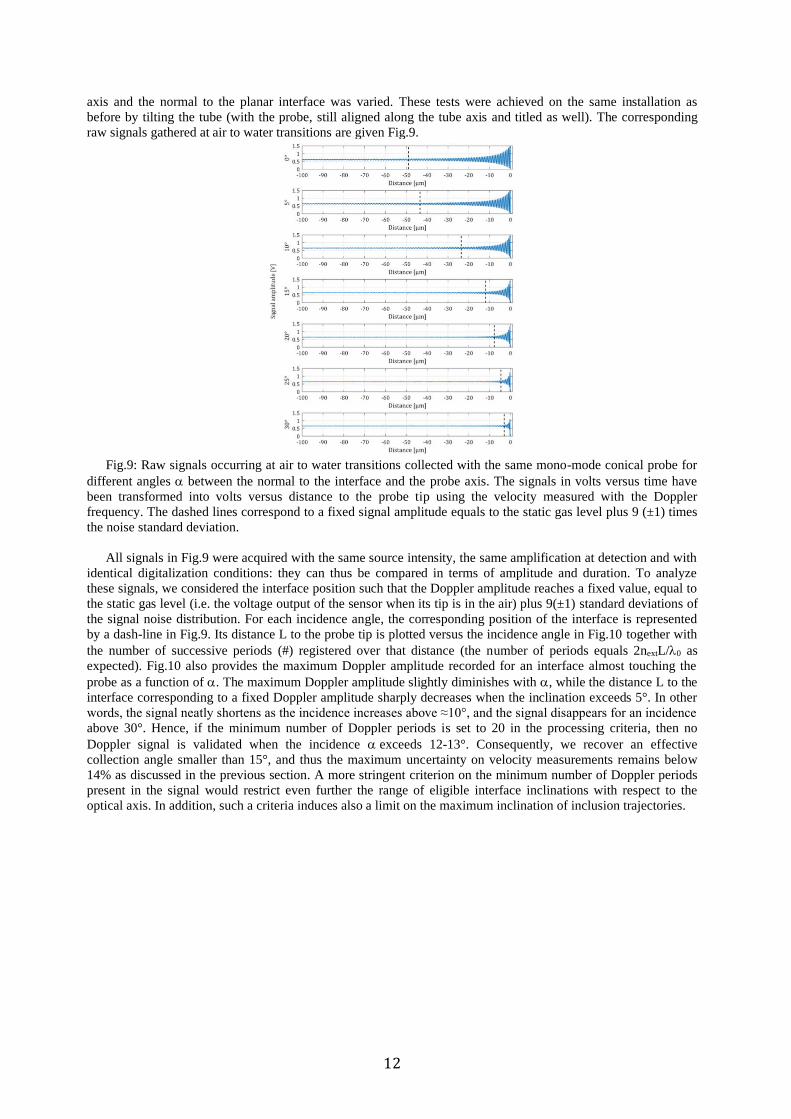
Fig.9: Raw signals occurring at air to water transitions collected with the same mono-mode conical probe for
different angles between the normal to the interface and the probe axis. The signals in volts versus time have
been transformed into volts versus distance to the probe tip using the velocity measured with the Doppler
frequency. The dashed lines correspond to a fixed signal amplitude equals to the static gas level plus 9 (±1) times
the noise standard deviation.
All signals in Fig.9 were acquired with the same source intensity, the same amplification at detection and with
identical digitalization conditions: they can thus be compared in terms of amplitude and duration. To analyze
these signals, we considered the interface position such that the Doppler amplitude reaches a fixed value, equal to
the static gas level (i.e. the voltage output of the sensor when its tip is in the air) plus 9(±1) standard deviations of
the signal noise distribution. For each incidence angle, the corresponding position of the interface is represented
by a dash-line in Fig.9. Its distance L to the probe tip is plotted versus the incidence angle in Fig.10 together with
the number of successive periods (#) registered over that distance (the number of periods equals 2nextL/0 as
expected). Fig.10 also provides the maximum Doppler amplitude recorded for an interface almost touching the
probe as a function of . The maximum Doppler amplitude slightly diminishes with , while the distance L to the
interface corresponding to a fixed Doppler amplitude sharply decreases when the inclination exceeds 5°. In other
words, the signal neatly shortens as the incidence increases above ≈10°, and the signal disappears for an incidence
above 30°. Hence, if the minimum number of Doppler periods is set to 20 in the processing criteria, then no
Doppler signal is validated when the incidence exceeds 12-13°. Consequently, we recover an effective
collection angle smaller than 15°, and thus the maximum uncertainty on velocity measurements remains below
14% as discussed in the previous section. A more stringent criterion on the minimum number of Doppler periods
present in the signal would restrict even further the range of eligible interface inclinations with respect to the
optical axis. In addition, such a criteria induces also a limit on the maximum inclination of inclusion trajectories.

13
Fig.10: Evolution with the angle between the normal to the interface and the probe axis, of the maximum
Doppler amplitude (in Volts) reached when the interface almost touches the probe, of the number of successive
Doppler periods in the signal (#) and of the distance (in µm) for which the Doppler amplitude remains higher than
9(±1) times the standard deviation of noise distribution.
Indeed, the results from Fig.9 and 10 can be exploited further to identify eligible bubble trajectories. For that,
the number of Doppler periods recorded as a function of the interface inclination has been represented as a
number of fringes versus the angle on the intensity map of Fig.4: Fig.11 indicates that the resulting boundary is
rather close to the 10-2 iso-contour in intensity. That boundary controls the trajectories compatible with a given
maximum extend of Doppler signals, or equivalently with a given number of periods. Clearly, from Fig.11, it
happens that only an inclusion travelling along the optical axis can produce a signal 60 periods long. If one
considers now shorter signals that are at least says n periods long, eligible trajectories are such that i) they are
fully within the dashed line iso-contour (that sets a minimum amplitude for Doppler signals) and ii) their
projection along the optical axis (here the horizontal) is at least n fringes long: the example shown Fig.11
corresponds to signals of at least 20 periods. Note that the projection is required because the velocity component
normal to the optical axis does not contribute to the Doppler shift. The above two conditions provide an upper
bound for the inclination of inclusion trajectories with respect to the optical axis: the maximum inclination is
plotted versus the number of Doppler periods in Fig.12 (for the selected Doppler amplitude). Clearly, as the
minimum number of required periods increases, eligible bubble trajectories become more and more aligned along
the optical axis. That trajectory selection has no consequence on measurement uncertainty because, as already
discussed, the latter is controlled by the inclination of the interface and by the orientation of the active wave
vector. Yet, that trajectory selection may have some consequences on the velocity statistics. Indeed, according to
Fig.12, if one sets a minimum of 10 fringes, the trajectory of the inclusion must make an angle within ±44° with
the optical axis. For a minimum of 20 fringes, that angular range decreases to ±28°. Similar effects are present in
LDV, and as for LDV, we will show in section 3.3 that velocity pdfs as measured by the new probe are almost
insensitive to signal processing parameters when the latter are properly selected.
20periods

14
Fig.11: On the intensity map of Fig.4, the open dots represent the number of fringes (or Doppler periods)
measured in controlled experiments when varying the angle at fixed amplitude of the Doppler signals. The red
dashed lines correspond to extreme bubble trajectories for a number of periods equal to 20.
Fig.12: Maximum inclination of eligible inclusion trajectories with respect to the optical axis as a function of
the number of periods recorded at an air to water transition. Here, the Doppler periods are considered only when
the Doppler amplitude exceeds a given threshold.
Another important issue related with velocity measurements concerns the ability of the sensor to detect
positive (i.e. corresponding to an inclusion approaching the fiber tip on its front) or negative (i.e. corresponding to
an inclusion approaching the fiber tip from the rear of the probe) velocities. This question is relevant since flow
reversal is commonly encountered in bubble columns operated in the heterogeneous regime. That feature has
prompted users to reconstruct pdfs from two data series recorded at the same position in the flow, one acquired for
a sensor pointing upward and another one from a sensor pointing downward (Xue et al. 2003, 2008; Chen et al.
2003). For these pdf reconstructions, it is usually argued that local probes do not detect gas inclusions arriving
from behind because of the presence of a (thick) probe holder. Yet, experimental evidences of that behavior are
scarce. In that perspective, we examined whether or not bubbles arriving from behind can produce exploitable and
meaningful Doppler signatures. A companion objective was to quantify a possible cross-talk error in the signal
interpretation. Two series of experiments were undertaken in that perspective.
A first series was achieved on quasi-planar interfaces, using gas slugs that were long enough to ensure the
complete de-wetting of the probe holder. Fig.13 provides the signals recorded by a downward directed probe
interacting with an ascending interface: the signals shown in the top row (cases a and b) correspond to the
standard situation of a probe impacting a bubble approaching head on. In the bottom row, Fig.13 provides signals
collected by the same probe but directed upward when an ascending slug goes through it: that inverted situation
corresponds to a bubble approaching the probe from the rear (signals c and d). Let us compare the signals
collected in these two situations. At liquid-to-gas transitions (left column in Fig.13), a weak Doppler signal is
present before the transition in the standard situation (case a). When the probe direction is inverted, a Doppler
signal still occurs at the liquid-to-gas transition but it is now located after the phase transition (case c). Concerning the passage from gas to liquid, a Doppler signal occurs before the transition in the standard situation (case b) but
none is recorded by an upward directed probe (case d). Hence, for bubbles larger than the tube holding the probe
that are able to de-wet the probe support, there is no risk to misinterpret the situation since the processing will
select Doppler signals arising at the gas level and preceding the gas-to-liquid transition (i.e. the signals
corresponding to case b in Fig.13).
Fig.13: Probe response when crossing an interface from air-to-water or from water-to-air with a probe oriented
along or against the gas slug velocity: a) and b) situations correspond respectively to bubble entry and bubble exit
for a bubble approaching the probe tip head-on. Situation c) - respectively situation d) - corresponds to a probe tip
entering - respectively exiting - a bubble approaching the probe tip from its rear.

15
A second series of experiments took place in a quasi-unidirectional bubbly flow produced in a 50mm I.D.
tube. Velocities were in the range 0.5-1m/s and bubble were 1 to 4 millimeters in size. Such dimensions are much
smaller than those of the probe holder: the full de-wetting of the probe support was thus unlikely. Velocity
statistics were gathered for a probe facing the main flow and for the same probe oriented at 180° from the main
flow direction. In the latter case, no Doppler signal was detected before gas-to-liquid transitions: consequently not
a single velocity data was acquired when the probe was at 180° from the main flow. To be very precise, let us
underline that a few Doppler signals were detected in that probe position, but they all occurred after the gas-to-
liquid transition and thus, they were not accounted for by the processing. Hence, whatever the bubble size
compared with the probe holder dimensions, the new sensor detects positive velocities only, where the term
positive corresponds here to an inclusion approaching the fiber and those direction goes from the probe tip to the
probe holder: this situation corresponds to the situation a) in Fig.13.
2.2.4 Probe-bubble interaction impact on velocity measurements
Finally, as the rear air/liquid interface of the bubble has been selected to analyze Doppler signals, it is worth
evaluating the impact of the probe-bubble interaction on the change in the bubble velocity. Probe-bubble
interaction has been analyzed for conical fibers used for phase detection (Vejrazka et al., 2010). The resulting
uncertainty on chord and concentration was shown to be controlled by the modified Weber number M=[ρL Db
ub2/] (Db/dprobe) where ub is the bubble approaching velocity with respect to the probe, dprobe the outer fiber
diameter, Db the bubble diameter, ρL the liquid density and the air-water surface tension (Vejrazka et al., 2010).
Typically, the uncertainty on void fraction remains below 10% for M higher than 50. Such a condition is easily
fulfilled in industrial bubble columns as these are usually operated at large superficial velocities so that the axial
fluid velocities exceed ≈0.2m/s over most of the column cross-section. In addition, the bubbles produced by
industrial spargers are typically larger than 2mm in diameter (Kantarci et al., 2005; Besagni et al., 2018; Chaumat
et al., 2007) so that their relative velocity is at least 0.2 m/s in fluids with a viscosity equal to or less than that of
water. These conditions correspond to bubble velocities with respect to the fixed probe of at least 0.4m/s and thus
to M higher than 50. Note that such conditions hold in the 0.4m I.D. bubble column exploited in section 4.
The modified Weber number M is also a key parameter controlling the bubble deceleration during its
interaction with the probe. More precisely, the change in the bubble velocity ∆ub at the time when the probe has
already pierced the bubble front interface and hits the bubble rear interface, compared with the undisturbed bubble
velocity ub was shown to be ∆ub/ub ≈ - 6 / [CAM 2/3 M], where the bubble aspect ratio is defined as the major
axis divided by the minor axis, and where CAM is the added mass coefficient (Vejrazka et al., 2010). Note that ∆ub
diminishes with the aspect ratio because of the strong decrease of CAM with . In air-water systems, ∆ub/ub
remains below 15% provided that the quantity CAM 2/3 M exceeds 40. That condition is indeed fulfilled in bubble
columns because M equals 50 (at least) as discussed above, and also because is larger than 1.2 as soon as
bubbles exceed 1.1-1.2 mm in size. Overall, the impact of the probe on the bubble slow down is at most -15%.
This estimation should be revisited for fluids more viscous than water.
To summarize the analyses presented in this section, the proposed sensor ensures accurate phase detection due
to its conical tip and its quite small latency length. It also provides information on velocity derived from the
Doppler signals formed at the gas-liquid interface and occurring just before the sensor extremity exits the bubble.
The measured velocity corresponds to the translation velocity of the gas inclusion projected along the probe
optical axis. Moreover, as bubbles arriving from the rear are easily discarded by the signal processing, only
positive velocities that correspond to inclusions approaching the front of the sensor are detected. The overall
uncertainty on velocity measurement has been evaluated to be at most 15% when considering both optical
detection conditions and probe-bubble interactions. For the latter, our estimate is grounded on a carrier phase
velocity of 0.2m/s: larger liquid velocities are usually encountered in bubble columns so that the bubble
deceleration should be significantly diminished. For example, for a carrier phase velocity of 0.4m/s, the modified
Weber number M is doubled and the change in bubble velocity decreases down to -8% instead of -15%.
Concerning the optical conditions, we have shown that imposing a higher threshold on the Doppler amplitude or
adding a requirement on the minimum number of Doppler periods changes the optical constraints and diminishes
further the uncertainty on velocity. On these bases, a signal processing routine has been developed to extract the
variables of interest. This processing is presented in the next section together with the sensitivity of measured
variables to the validation criteria introduced in that processing.
3. Signal processing, sensitivity to processing parameters and sensor performances
To develop the processing and to test the performances of the sensor, data were acquired in bubbly flows
produced in a 3m high bubble column with an internal diameter D=2R=0.4m. The column was filled with tap
water at an initial height of 2.02m. Dried air was injected through 352 orifices (1mm in diameter, 10mm long)
uniformly distributed over the cross-section S. The injected gas flow rate QG was varied from 100 to 1900 Nl/min,
so that the superficial velocity Vsg=QG/(πR2) ranged from 1.3cm/s to 35cm/s. All data were collected at H=1.45m

16
above injection, i.e. for H/D=3.62 a position within the quasi fully developed region (Maximiano Raimundo et al.,
2019). Unless otherwise stated, the Doppler probe was vertical and downward oriented. The probe was immerged
in the bubble column from the top using a metallic square bar (side 20mm) to avoid vibrations: to reduce the flow
perturbation, the probe was located 55mm away from that bar and parallel to it.
As for classical optical probes, the signal delivered by the Doppler probe consists in a succession of crenel-like
modulations, each one corresponding to a bubble pierced by the sensor (Fig.14). The goal of the processing is to
determine the arrival time tA, the exit time tE and thus the gas dwell time TG = tE-tA of each detected bubble (Fig.3)
and to evaluate its velocity from the Doppler modulation when the latter is present.
Fig.14: Raw signals from the Doppler probe (a) and examples of partial amplitude signals (b).
3.1 Phase detection routine
To identify the bubbles hitting the probe, we adapted the signal processing developed for classical optical
probes and already tested in diverse flow conditions (Barrau et al., 1999). First, as the liquid level is quite stable,
any signal exceeding the noise at the liquid level is considered to be a contribution from a gas inclusion.
Accordingly, the detection routine uses an absolute threshold in amplitude: this lower threshold is typically set at
the liquid level plus half the peak-to-peak noise amplitude. Second, as Doppler modulations must not be
interpreted as gas inclusions, we introduced an upper threshold in amplitude that is higher than the lower threshold
(Fig.3). As seen in section 2.1, the amplitude dynamics of the signal is set by the Fresnel coefficient times I0. The
liquid level AL corresponds to a fully wetted probe for which Rfiber/water ≈ 0.0025. The plateau at the gas level AG is
obtained when the entire latency length has been dried off: it corresponds to Rfiber/air ≈ 0.036. Thus the signal
dynamics ∆A=AG-AL corresponds to 0.033 I0. Meanwhile, the amplitude of a Doppler signal at a water-to-air
transition amounts to 0.007 I0 that is roughly to 21% of ∆A. At an air-to-water transition, the Doppler amplitude is
larger: it amounts to 0.026 I0 that is about 77.6% of ∆A. These estimates are optimistic as we assume here normal
incidences, and we do not account for any geometrical factor connected with light diffusion on the interface or
with light collection back in the fiber. Actual Doppler amplitudes are therefore expected to be significantly smaller than the above figures. Concerning bubble detection, when a Doppler occurs before the water-to-air
transition as in Fig.3-left, the amplitude of the signal is at most AL + (0.21/2) ∆A= AL+0.1 ∆A. Thus, setting an
upper threshold above that limit ensures the detection of the gas inclusion without interpreting Doppler
oscillations as bubbles. The arrival time tA of the gas inclusion is then found by going back in time to the first
event whose amplitude is close to the lower threshold: this process is represented by the red arrow leading to the
event A in Fig.3-left.
At the gas-to-liquid transitions (Fig.3-right), the Doppler amplitude is stronger (≈78% of the signal dynamics)
but it never reaches the liquid level. Therefore, any threshold below AL + (1-0.78/2) ∆A = AL + 0.61 ∆A allows
detecting the gas-to-liquid transition while escaping the Doppler signal. Consequently, either an upper below
AL+0.61∆A or the lower threshold as defined above can be used to capture the sharp gas-to-liquid transition. To
identify the time tE corresponding to bubble exit, one has to go back in time to the first event those amplitude
reaches the gas plateau: the red arrow leading to the event E in Fig.3-right represents that search. Hence, Doppler
oscillations are not accounted for in gas detection, and the gas dwell time 𝑡𝐺𝑖 of the ith bubble is tE - tA.
The above phase detection routine is well adapted to signals with a plateau at the gas level such as the one
shown Fig.3. As the latency length of the Doppler probe is very small compared with usual bubble sizes (the latter
are typically above 0.5mm in most industrial processes), nearly all bubble signatures do reach a plateau at the gas
level. From a long record collected on the column axis at Vsg=3.3cm/s, we indeed observed that 98.6% of the
bubbles signatures reach the plateau at the gas level. Yet, not all these signals provide a Doppler modulation: this
is because of the angular constraints discussed in section 2.2. In addition, the 1.4% remaining events collected by
the probe corresponds to signals of very small amplitude: examples are provided Fig.14-right. Such events occur
when the probe extremity is not fully de-wetted during the passage of a gas inclusion. In the flows considered
here, the bubble size is always much larger than the latency length. Therefore, all signatures of reduced amplitude
correspond to tangential hits, i.e. to very small chords, of the order of the latency length, cut through larger
inclusions (Vejrazka et al., 2010; Cartellier, 1992). For such signatures, the gas entry is detected as described
above. For the gas exit, since these signatures are most of the time smoothly decaying in time after having reach
their peak amplitude, the date of the peak is usually considered as the gas exit. For the Doppler optical probe,
these low amplitude signals are rare and they bring a negligible contribution to the void fraction. At Vsg=3.3cm/s,
they amount for 9 10-5 in absolute value to be compared with the mean void fraction of 0.15. In addition, these
a) b)

17
small signatures, whose amplitude is at most 30-40% of the signal dynamics, never provide Doppler signals.
Therefore, only the fraction of these small signals whose maximum amplitude is below the upper threshold is
discarded by the processing.
3.2 Phase detection efficiency
The sensitivity to threshold selection was analyzed on a signal collected on the column axis at Vsg=19.5cm/s,
i.e. in the heterogeneous regime. The 348 seconds long record (more than 40000 bubbles detected) ensures the
convergence of the void fraction within ±0.0044 of void for a mean void fraction equal to 0.335. The liquid level
was 7mV with a peak-to-peak noise about 23mV: the lower threshold was set at 25mW, i.e. slightly above the
minimum recommended of 18.5mV. The gas level was 0.9 Volts just after piercing and it smoothly decreased in
time down to its plateau value at about 0.8 Volts (see Fig.15) because of the thinning of the liquid film attached to
the probe tip. Hence, according to the recommendation given in the previous section, the upper threshold should
remain below 0.55mV. However, since the signals experienced strong overshoots (up to 1.5V) at the gas-liquid
transition, we extended the sensitivity analysis outside the recommended range, and the upper threshold was
varied from 26mV up to 1.5V. The analysis was repeated for a lower threshold twice as large (50mV) and for
upper thresholds between 100mV and 1.5V. The evolution of the local void fraction versus the two thresholds
presented Fig.15 shows that the void fraction remains almost insensitive to the threshold selection. Quantitatively,
the maximum difference amounts to 1.5 10-3 in absolute void fraction (less than 0.4% in relative value) when the
upper threshold evolves within the recommended range. That result also holds for an upper threshold up to 1.2V:
this is because the detection criterion is not absolute but it is conditional. Indeed, whenever a bubble signature is
detected, the processing goes back to the entry point A defined by the lower threshold (Fig.3). The exact value of
the upper threshold is therefore irrelevant provided that the presence of a bubble signature has been detected. This
is no longer true above 1.2V because not all overshoots reach such a voltage, and this is why the void fraction and
the number of detected bubbles decrease for an upper threshold between 1.2V and 1.5V. Similar results are
obtained when doubling the lower threshold (i.e. 50mV): this is because, for the signals considered, the peak-to-peak noise remains stronger than the Doppler amplitude at water-air interfaces. Overall, the void fraction and the
number of detected bubbles happen to be almost insensitive to the upper threshold when the latter is selected
within a wide interval, ranging from 10% to 60% of the signal dynamics. Moreover, we also found that the gas
residence time distribution remains the same when the thresholds evolve within the recommended range. We
further compare with the void fraction on the column axis detected by a classical conical probe those latency
length was about 40µm: from Vsg=0.3 to 25cm/s, the gas hold-up difference in relative value between the two
sensors was in average 3% with a maximum at 6%. Hence, according to these tests, the Doppler sensor happens to
be quite reliable in terms of gas phase detection.
Fig.15: Typical bubble signature (top) and evolution of the void fraction versus the upper threshold for two
lower thresholds (bottom). Signal 348 seconds long collected on the bubble column axis for Vsg=19.5 cm/s.
3.3 Velocity measurement
Once individual bubbles are identified, Doppler bursts are searched before each phase transition. That search is
performed over a time window evaluated from an a priori estimate of the minimum expected velocity and for a
given number of periods. The extent of the search window is also bounded by the previous phase transition. The
raw signals are digitalized at a sampling frequency fsampling at least twice (owing to Nyquist criteria) the maximum
Doppler frequency fDmax corresponding to the largest velocity in the flow. In practice, fsampling is often set to five
times fDmax. The default value for the minimum velocity is set to fsampling/500: it defines the lowest Doppler
frequency fDmin that can be detected. A Fourier transform is then performed over the working window to identify
potential Doppler bursts within the interval [fDmin, fDmax]. For that, use is made a Butterworth filter of order 2 those

18
-3dB bandwidth is [fHP, fLP]. The default values are fLP=fDmin=fsampling/5 and fHP = fDmax = fsampling/500. Both fLP and
fHP can be selected at will: their impact is examined in section 3.3.2.
In the case of a true Doppler burst, a clear maximum is found in the Fourier transform and that peak frequency
is extracted. For the final analysis, one goes back to the temporal signal. First, the raw signal is band-pass filtered
around that peak frequency with a Butterworth filter of order 2 those -3dB bandwidth is set at 0.2 and 1.8 times
the peak frequency to remove both some noise at high frequencies and the baseline component at low frequencies.
Such a filtered Doppler signal is exemplified Fig.16. On that filtered signal, successive fringes are identified using
a local maxima search. An instantaneous period is computed for each fringe as the elapsed time between
successive local maxima. The Doppler burst is validated only if one can find n consecutive periods those values
are the same within %, with ranging from 5 to 20%. When it is so, the velocity Vi of the 𝑖th bubble is computed
from eq.(1) using the average period determined over the n oscillations: the selection of suitable values of n and
is discussed in section 3.3.2. Let us underline that experiments in bubbly flows have shown that the Doppler
frequency is often decreasing when a water/air interface is approaching, possibly because of liquid inertia and
localized interface deformation. With usual optical fibers, the interface deformation at a water-to-air transition gas
is about 7-11µm for velocities below 10m/s (Liju et al., 2001): such a magnitude is compatible with the present
observations since the decrease in frequency is typically observed over a few fringes (Fig.6). To get rid of that, the
search for the n successive periods starts between 0 to 5 fringes away from the probe-interface contact. From now
on, all the results presented exploit the Doppler modulation detected at air-to-water transitions (next =1). Hence,
the final information provided by the signal processing consists in the arrival time and the gas dwell time of all
detected gas inclusions plus the velocity for a subset of these bubbles. This is the same information available
collected from multimode fiber probes, and thus, the same post-processing can be applied to extract variables of
interest including concentration, number density, fluxes and interfacial area density (Cartellier, 1999).
Fig.16: On a band-pass filtered Doppler burst (blue curve) observed before gas-liquid transition, fringes are
identified (black dots) and assigned an instantaneous frequency value (red curve). The probe-interface contact is
located at the extreme right of the signal: the search for consecutive fringes starts between 0 to 5 fringes away
from that contact. The bold portion of the red curve corresponds to n=30 consecutive fringes with the same period
within =: it is exploited to compute the average frequency and the bubble velocity.
To investigate the sensitivity of velocity measurements to the four processing parameters, namely n, and the
filter bandwidth [fHP, fLP], we considered one superficial velocity in the homogeneous regime and another one in
the heterogeneous regime. The main characteristics of the signals and of the processing are given Table 2: both
records were long enough to ensure a satisfactory convergence. For that analysis, we considered the statistics built
on detected velocities only without using any interpolation scheme to evaluate missing velocity data.
Measuring conditions Homogeneous conditions
Vsg = 1.3 cm/s
Heterogeneous conditions
Vsg = 16.25 cm/s
Record duration 837 seconds 95 seconds
Number of bubbles detected 9315 9143
Liquid level 10 mV 10 mV
Gas level 0.86 Volts 1.02 Volts
Peak to peak noise amplitude at liquid level 10 mV 15 mV
Peak to peak noise amplitude at gas level 50 mV 50 mV
Lower detection threshold 50 mV 50 mV
Upper detection threshold 0.56 V 0.68 V
Sampling frequency 62.5 MHz 62.5 MHz
High pass frequency fHP - Low pass frequency
fLP (dynamic range of the filter fLP/ fHP)
140 kHz – 2137 kHz
(dynamic range 15.3)
140 kHz – 6250 kHz
(dynamic range 44.6)

19
Table 2: Conditions exploited to investigate the sensitivity of velocity measurements to processing parameters.
3.3.1 Optimum choice of n and
We examined first the mean bubble velocity and its standard deviation for a number n of periods ranging from
10 to 100 and for a maximum deviation between 2% and 25%. The reference values are set to n=20 and =10%:
they correspond to standards in Laser Doppler Velocimetry. For the heterogeneous regime, the deviation (in %)
from the reference is provided Table 3. It is color-coded: white data are within ±5% of the reference, grey data
within ±10% and dark grey data correspond to deviations above ±10%. Clearly, there is always a significant range
of processing parameters over which the measurements remain nearly the same. The mean velocity is recovered
within ±5%, for between 10% and 20% and for n from 20 to 75. When considering the standard deviation, that
interval slightly diminishes to between 10% and 15%. Similar results (not shown) were obtained in the
homogeneous regime. Hence, high fidelity measurements are ensured provided that n and remain within the
above-mentioned intervals.
The largest (above 15-20%) deviations systematically occur for extreme values of n and . That occurs when
is too small (≤ 2%) resulting in a too strong selection of “stable” Doppler signals, or when is too large (≥ 25%)
in which case the noise is easily interpreted as a Doppler signature. That also arises for n below 20: in that case,
the search for short Doppler signals favors the validation of noise (see Fig.18 and the associated discussion). The
worst cases occur for a small number of periods (n=10) and for in the upper portion of its range (20-25%): the
deviation increases up to 30-60% for the mean velocity and it could exceed 100% for the standard deviation.
Table 3: Deviation in % from the reference value of the mean inclusion velocity (top) and of its standard deviation
(bottom) to processing parameters (Heterogeneous regime Vsg=16.25 cm/s, signal characteristics as in Table 2).
The validation rate, defined as the fraction of detected bubbles for which information on velocity is directly
available, is shown Fig.17 as a function of n and . It monotonously decreases with n, i.e. when increasing the
minimum duration of Doppler bursts. Whatever n, it is almost unaffected by for between 10% and 20% but it
drastically drops for below 5%: such trends are similar to those observed in LDV response (Durst et al., 1976).
To maximize the validation rate while ensuring a good fidelity, selecting n=20 periods and =10% seems to be an
optimal choice. For these values, the validation rate reaches 66% in homogeneous conditions, and it decreases
down to about 50% in heterogeneous conditions, probably because of the complex bubble trajectories in that
regime. Let us note that all the results presented in this section correspond to a probe pointing downward, that
only detects bubbles moving upward. The detection of bubbles flowing downward will be examined in section 4.
Periodhomogeneity->
numberofperiods:25% 20% 15% 10% 5% 2%
10 60.03 28.64 6.33 0.67 2.17 16.15
20 29.09 4.46 0.88 0.00 3.02 20.82
30 14.41 1.51 0.07 0.64 5.63 23.57
40 7.99 0.57 1.73 4.09 6.30 22.10
50 1.82 1.42 2.91 3.39 6.21 22.48
75 0.19 2.48 3.81 4.19 6.69 28.72
100 0.07 3.97 5.46 5.97 5.81 29.85
Periodhomogeneity->
numberofperiods:25% 20% 15% 10% 5% 2%
10 166.48 106.40 33.09 5.64 3.74 25.95
20 106.28 21.88 4.49 0.00 3.81 35.69
30 64.07 11.26 4.50 0.60 6.98 42.60
40 41.91 6.56 2.23 1.49 9.06 44.49
50 18.58 5.71 2.39 2.26 11.59 48.82
75 11.88 2.07 0.10 4.21 14.86 56.64
100 12.23 3.38 0.94 7.86 14.31 56.75
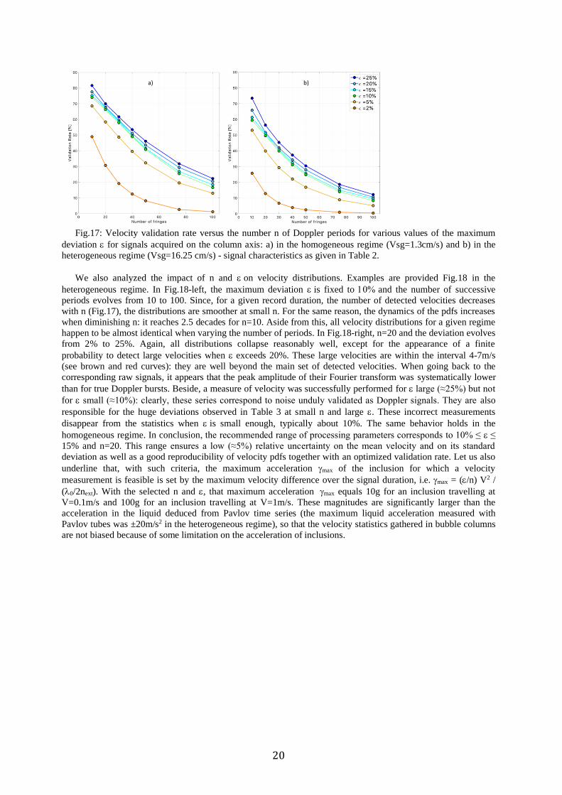
20
Fig.17: Velocity validation rate versus the number n of Doppler periods for various values of the maximum
deviation for signals acquired on the column axis: a) in the homogeneous regime (Vsg=1.3cm/s) and b) in the
heterogeneous regime (Vsg=16.25 cm/s) - signal characteristics as given in Table 2.
We also analyzed the impact of n and on velocity distributions. Examples are provided Fig.18 in the
heterogeneous regime. In Fig.18-left, the maximum deviation is fixed to and the number of successive
periods evolves from 10 to 100. Since, for a given record duration, the number of detected velocities decreases
with n (Fig.17), the distributions are smoother at small n. For the same reason, the dynamics of the pdfs increases
when diminishing n: it reaches 2.5 decades for n=10. Aside from this, all velocity distributions for a given regime
happen to be almost identical when varying the number of periods. In Fig.18-right, n=20 and the deviation evolves
from 2% to 25%. Again, all distributions collapse reasonably well, except for the appearance of a finite
probability to detect large velocities when exceeds 20%. These large velocities are within the interval 4-7m/s
(see brown and red curves): they are well beyond the main set of detected velocities. When going back to the
corresponding raw signals, it appears that the peak amplitude of their Fourier transform was systematically lower
than for true Doppler bursts. Beside, a measure of velocity was successfully performed for large (≈25%) but not
for small (≈10%): clearly, these series correspond to noise unduly validated as Doppler signals. They are also
responsible for the huge deviations observed in Table 3 at small n and large . These incorrect measurements
disappear from the statistics when is small enough, typically about 10%. The same behavior holds in the
homogeneous regime. In conclusion, the recommended range of processing parameters corresponds to 10% ≤ ≤
15% and n=20. This range ensures a low (≈5%) relative uncertainty on the mean velocity and on its standard
deviation as well as a good reproducibility of velocity pdfs together with an optimized validation rate. Let us also
underline that, with such criteria, the maximum acceleration max of the inclusion for which a velocity
measurement is feasible is set by the maximum velocity difference over the signal duration, i.e. max = (/n) V2 /
(0/2next). With the selected n and , that maximum acceleration max equals 10g for an inclusion travelling at
V=0.1m/s and 100g for an inclusion travelling at V=1m/s. These magnitudes are significantly larger than the
acceleration in the liquid deduced from Pavlov time series (the maximum liquid acceleration measured with
Pavlov tubes was ±20m/s2 in the heterogeneous regime), so that the velocity statistics gathered in bubble columns
are not biased because of some limitation on the acceleration of inclusions.
a) b)

21
Fig.18: Evolution of bubble velocity distributions as a function of the parameters n and e
eterogeneous regime (Vsg=16.25cm/s): a) impact of the number of periods n from 10 to 100 for a fixed
deviation =10%, b) impact of the deviation from 2% to 25% for a fixed number of periods n=20 - Signal
characteristics as given in Table 2 - fHP=140 kHz.
3.3.2 Optimum choice of filters
The parameters n and being set, the settings of the band-pass filter [fHP ; fLP] are worth to be examined, as we
have seen that incorrect velocity data can be extracted from noise. Concerning the low pass frequency fLP that
controls the upper limit in velocity, the maximum velocity is correctly detected when fLP is higher than about 0.8
times the highest Doppler frequency fDmax in the record (this 0.8 coefficient is slightly less than unity because of
the shape of the filter). Concerning the lower velocity limit, low velocities progressively disappear from the pdfs
as fHP increases: the cut-off occurs at a frequency about 0.8-0.9 times fHP, in agreement with the characteristics of
the Butterworth filter. However, we also analyzed the impact of the actual velocity dynamic range on these limits
using signals collected in the homogeneous and in the heterogeneous regimes. The following trends were sorted
out from this investigation (see Mezui M’Obiang Y., 2021 for more details):
• The detection of the maximum velocity is rather straightforward. Whatever the filter dynamic with respect to
the actual velocity, the maximum velocity is successfully determined provided that the low pass filter is such
that fLP/fD max ≈ 1 so that the highest velocities in the signal are not rejected. More precisely, fLP/fD max ≥ 0.8
suffices for an accurate detection of the true maximum. Note also that fLP should not be increased too much as
the detection of the maximum velocity deteriorates if the low pass frequency exceeds more than about three
times the maximum Doppler frequency in the signal.
• The detection of the minimum velocity remains accurate, unless the low-pass frequency is too high compared
with the maximum Doppler frequency, say for fLP/fDmax ≥ 1.3. Also, low velocities data start to be lost when,
for a given low pass filter, the dynamic range of the band-pass filter becomes too small compared with the
actual frequency dynamics in the signal. To correctly detect the minimum velocity when fLP/fDmax = 0.8, the
filter dynamic fLP/fHP should be at least equal to the actual frequency dynamics in the signal.
When these recommendations are fulfilled, the validation rate happens to be maximized. We also checked that
the mean velocity VG and its standard deviation VG’ are nearly unaffected by the filter settings when the latter are
properly chosen. For example for a low-pass filter set at fLP/fD max=0.8 and for a filter dynamics fLP/fHP between 1
and 10 times the actual signal dynamics, the variation is 0.25% on VG and 1.4% on VG’ in the homogeneous
regime. In the heterogeneous regime, the variation is 4.9% on VG and 1.55% on VG’. All these figures represent
quite acceptable sensitivities.
Let us also underline that the discussion on n and parameters was achieved for a high pass frequency fHP set
to 140kHz (Table 2). That choice was indeed within the recommendations made on the filters settings as the filter
dynamics was 1.36 times the frequency dynamics in the signal for the homogeneous regime (and 1.1 times for the
heterogeneous regime). Therefore, the recommendations made for n and correspond to true optimal values that
are not filter dependent.
At this stage, it is interesting to comment on extreme values of the measured velocity. Over a record of 4500
valid velocity measurements in heterogeneous condition, two data were found at 7m/s (see Fig.19). If these data
are set apart, the next largest velocity detected is about 5m/s, a value that corresponds to the visual limit of the
a) b)
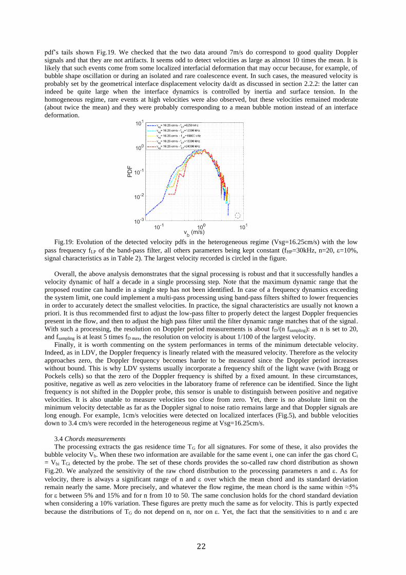
22
pdf’s tails shown Fig.19. We checked that the two data around 7m/s do correspond to good quality Doppler
signals and that they are not artifacts. It seems odd to detect velocities as large as almost 10 times the mean. It is
likely that such events come from some localized interfacial deformation that may occur because, for example, of
bubble shape oscillation or during an isolated and rare coalescence event. In such cases, the measured velocity is
probably set by the geometrical interface displacement velocity da/dt as discussed in section 2.2.2: the latter can
indeed be quite large when the interface dynamics is controlled by inertia and surface tension. In the
homogeneous regime, rare events at high velocities were also observed, but these velocities remained moderate
(about twice the mean) and they were probably corresponding to a mean bubble motion instead of an interface
deformation.
Fig.19: Evolution of the detected velocity pdfs in the heterogeneous regime (Vsg=16.25cm/s) with the low
pass frequency fLP of the band-pass filter, all others parameters being kept constant (fHP=30kHz, n=20, =10%,
signal characteristics as in Table 2). The largest velocity recorded is circled in the figure.
Overall, the above analysis demonstrates that the signal processing is robust and that it successfully handles a
velocity dynamic of half a decade in a single processing step. Note that the maximum dynamic range that the
proposed routine can handle in a single step has not been identified. In case of a frequency dynamics exceeding
the system limit, one could implement a multi-pass processing using band-pass filters shifted to lower frequencies
in order to accurately detect the smallest velocities. In practice, the signal characteristics are usually not known a
priori. It is thus recommended first to adjust the low-pass filter to properly detect the largest Doppler frequencies
present in the flow, and then to adjust the high pass filter until the filter dynamic range matches that of the signal.
With such a processing, the resolution on Doppler period measurements is about fD/(n fsampling): as n is set to 20,
and fsampling is at least 5 times fD max, the resolution on velocity is about 1/100 of the largest velocity.
Finally, it is worth commenting on the system performances in terms of the minimum detectable velocity.
Indeed, as in LDV, the Doppler frequency is linearly related with the measured velocity. Therefore as the velocity
approaches zero, the Doppler frequency becomes harder to be measured since the Doppler period increases
without bound. This is why LDV systems usually incorporate a frequency shift of the light wave (with Bragg or
Pockels cells) so that the zero of the Doppler frequency is shifted by a fixed amount. In these circumstances, positive, negative as well as zero velocities in the laboratory frame of reference can be identified. Since the light
frequency is not shifted in the Doppler probe, this sensor is unable to distinguish between positive and negative
velocities. It is also unable to measure velocities too close from zero. Yet, there is no absolute limit on the
minimum velocity detectable as far as the Doppler signal to noise ratio remains large and that Doppler signals are
long enough. For example, 1cm/s velocities were detected on localized interfaces (Fig.5), and bubble velocities
down to 3.4 cm/s were recorded in the heterogeneous regime at Vsg=16.25cm/s.
3.4 Chords measurements
The processing extracts the gas residence time TG for all signatures. For some of these, it also provides the
bubble velocity Vb. When these two information are available for the same event i, one can infer the gas chord Ci
= Vbi TGi detected by the probe. The set of these chords provides the so-called raw chord distribution as shown
Fig.20. We analyzed the sensitivity of the raw chord distribution to the processing parameters n and . As for
velocity, there is always a significant range of n and over which the mean chord and its standard deviation
remain nearly the same. More precisely, and whatever the flow regime, the mean chord is the same within ≈5%
for between 5% and 15% and for n from 10 to 50. The same conclusion holds for the chord standard deviation
when considering a 10% variation. These figures are pretty much the same as for velocity. This is partly expected
because the distributions of TG do not depend on n, nor on . Yet, the fact that the sensitivities to n and are

23
similar for chords and for velocities means that there is no significant correlation between velocity and gas dwell
time measurements: in other words, no bias in gas velocity statistics is to be expected from the Doppler probe.
Fig.20: Evolution of raw chord distributions (i.e. without velocity interpolation) with n for a fixed =10%: a)
in the homogeneous regime (Vsg=1.3cm/s) and b) in the heterogeneous regime (Vsg=16.25cm/s). Signal
characteristics as given in Table 2 with fLP=92kHz, fHP=1.005MHz for the homogeneous condition, and with
fLP=146kHz, fHP=3.751MHz for the heterogeneous condition.
As shown Figure 20-right, the minimum chord directly detected (i.e. with direct velocity measurements)
increases with the number n of periods. This is indeed expected as a valid velocity measurement requires a
minimum number n of successive periods, that is a minimum signal duration within the gas phase: that duration
corresponds to a length L = n 0/(2next). L is about 8µm for the smallest n considered (n=10): this is larger than the
latency length LS, so that the corresponding signals exhibit a flat plateau at the gas level and a neat Doppler
modulation. Consequently, L also represents the shortest chord that can be detected with direct velocity detection.
The only puzzling result we observed concerns the maximum chord detected in the heterogeneous regime. The
latter nearly reaches 10cm at Vsg=16.25cm/s, to be compared with a mean chord about 4mm and a standard
deviation about 7mm. That result was insensitive to n, and to filter limits. We scrutinized the flow inside the
column with an endoscope. The key point is that no bubbles with such sizes were present in the column: the
largest bubble ever observed was 9mm in size. The huge chords detected with the probe represent a few percent of
the total population. A close examination of the associated signals indicates that more than 60% of these
unambiguously show multiple bubbles, as illustrated Figure 21. If one considers successive bubbles separated by a
liquid film that is thinner than the probe latency length, then, the signal will never reach the liquid level.
Consequently, a single bubble would be detected with a gas residence time equal to the sum of all constitutive gas
dwell times. In Figure 21, that process concerns 3 bubbles in signal a) and 6 (and possibly more) bubbles in the
signal b). It is therefore highly likely that the huge chords detected in heterogeneous conditions do arise because
of close-by bubbles that are not individually distinguished by the probe. The companion question is where do
these close-by bubbles come from? It is likely that such events correspond to bubbles trapped in the core of very
intense vortices that form in the strongly sheared regions of the flow, the latter being the consequence of unsteady
large-scale motions arising in the heterogeneous regime (Maximiano Raimundo et al., 2019). Indeed, zones at
high void fraction, up to ten times or more the mean gas hold-up, do exist in the heterogeneous regime
(Maximiano Raimundo et al., 2019) and that may explain how multiple bubbles can be artificially associated to
provide apparent very long chords. The detection of such large chords remains rare enough, so that they do not
alter the mean chord but they significantly contribute to the standard deviation. To quantify this effect, we
considered the contribution of chords larger than the mean value CG plus two standard deviations CG’. In the
heterogeneous regime at Vsg=16.25cm/s, CG=4mm and CG’=7.6mm. The chords above CG+2CG’=19mm
represent 3% of the population: their contribution to the mean value is 3% while their contribution to the standard
deviation amounts to 20%. In conclusion, and as for velocity, the recommended processing parameters ensure a
reasonable uncertainty on the mean chord and on its standard deviation as well as a good reproducibility of raw
chord distributions.
a) b)

24
Fig.21: Signals corresponding to long gas chords collected in the heterogeneous regime: top) chord = 43mm at
a velocity ≈ 1.6 m/s; bottom) chord = 84mm at a velocity ≈ 1.4 m/s.
4. First exploitation of the Doppler probe in a bubble column operated in the heterogeneous regime
To test the capabilities of the Doppler probe, we exploited that sensor in an air/water bubble column operated
in the heterogeneous regime in order to gather some new information. The experiments were performed in a 3m
high bubble column with an internal diameter D=0.4m. The static liquid height was fixed to 2.02m that is about
5D, and the measurements were collected in the quasi fully developed region of the flow (Maximiano Raimundo
et al., 2019). Beside, all the results discussed in section 3 were gathered with a vertical and downward oriented
probe. However, it is known that heterogeneous conditions are associated with large velocity fluctuations. In
particular, and especially off axis, the liquid can experience downward directed motion over significant periods of
time. As the Doppler sensor is not responding to negative velocities, it is thus essential to acquire information
from an upward oriented probe and to combine it with the information gathered from a downward oriented probe.
Xue et al., 2008 used a similar procedure with four-tip sensors. Let us examine its relevance for Doppler probes.
4.1 Sensitivity to the main flow orientation and measurements of bubble velocity pdfs
To complement the tests presented in section 2.2.3, let us first analyze the sensitivity of velocity measurements to
probe orientation in the complex bubbly flows arising in a bubble column. These measurements were collected at
H/D=3.62 above injection, where the flow is quasi fully developed. In these experiments, the optical fiber was
inserted in a 0.9mm internal diameter and 1.5mm outer diameter stainless steel tube, and the fiber protruded 7 mm
out of the tube. To avoid vibrations of the sensor, this tube was held on a 9° wedge support (10mm thick, lateral
extension 60mm long), itself fixed at the extremity of a square (width 20mm) metallic bar immersed in the
column from the top. The tube was located at the extremity of the wedged support (55mm away from the vertical
bar), and the optical tip of the probe was 76mm ahead of the wedge. Signals were collected with the same probe downward and then upward oriented. They were treated using optimum filters and standard values for n and
he results are provided Table 4.
Table 4: Statistics gathered from the same probe using downward and upward orientations at H/D=3.625. The
values presented correspond to a filter dynamic that is twice the signal dynamic defined at the 1‰ limits.
In the homogeneous regime (Vsg=1.3cm/s), all bubbles are travelling upward in a laboratory frame. They thus
produce head-on impacts on a downward oriented probe. Consequently, the velocity validation rate is high: here,
it equals 66.5%. When the same probe is oriented upward, two effects are noticeable:
- First, there is a decrease in the detection frequency compared with a downward directed probe. This is
probably due to the rather thick probe holder used here that alters some bubble trajectories and thus hampers the
correct detection of all incoming bubbles. Here, an upward directed probe detects 64% of incoming bubbles: that
Flow conditions
Radial position
Probe orientationdownward
directed probe
upward directed
probe
downward
directed probe
upward
directed probe
downward
directed probe
upward
directed probe
Number of inclusions detected 9297 6007 9143 6766 10505 3708
Measuring duration 837 s 850 s 95 s 95 s 221.8 s 95 s
Detection frequency Hz 11.1 7.1 96 Hz 71 Hz 47 Hz 39 Hz
Velocity validation rate 66.5% 0% 52.1% 1.27% 26.7% 17.8%
Mean velocity m/s 0.44 - 1.2 - 0.40 0.86 - 0.51
Mean chord mm 2.7 - 4.10 1.86 3.67 2.34
Volumetric flux (m/s) 0.026 - 0.208 0.0027 0.0548 0.0177
Homogeneous (Vsg= 1.3 cm/s) Heterogeneous (Vsg=16.25 cm/s)
On axis On axis 0.7 R

25
is the decrease in the detection capability due to an inverted probe orientation amounts to 36%. The decrease in
terms of void fraction is of the same order, about 40%.
- Second, when the probe is upward oriented, the velocity validation rate drastically drops. In the example of
Table 4, no Doppler signal was collected among more than 6000 bubbles detected. In another record, the interface
velocity was measured on a single event out of 2563: that corresponds to a 0.04% success rate. These results
confirm the conclusion of Section 2, namely that the Doppler probe is unable to detect negative velocities with
respect to the probe orientation.
In the heterogeneous regime, and depending on Vsg and on the radial location, the liquid and/or the bubbles
can experience both up and down motion in a frame attached to the column (Xue et al., 2008; Maximiano
Raimundo et al., 2016; Guan et al., 2017). For that reason, the response of the probe was analyzed at two
locations, on the axis of the bubble column and at a lateral position x/R=0.7 where the mean liquid velocity is
close to zero. The investigation was done at Vsg =16.25cm/s.
- On the column axis, the detection frequency decreases from 96Hz to 71Hz when the probe is inverted with
respect to the mean flow. According to the liquid velocity pdf collected from a Pavlov tube shown Figure 22, the
liquid flow on the axis is upward directed 96% of the time. Therefore, and as in homogeneous conditions, the
decrease in the detection frequency is most probably due to the probe holder that hampers the detection of some of
the incoming bubbles. For the holder used and the flow conditions considered in Table 4, the decrease in the
detection frequency when using an inverted probe orientation amounts to 26%. In terms of void fraction, the
decrease is 10 to 20%: these figures are slightly less than in the homogeneous regime.
- We have just seen that negative liquid velocities are recorded 4% of the time on the axis, and that their
magnitude is up to 0.5m/s (Fig.22). Such velocities are strong enough to entrain some bubbles downward. When
the Doppler probe is upward directed, it indeed detects a few meaningful Doppler signals that amount for 1.27%
of the number of detected bubbles (Table 4): these signals represent 86 events out of 6766 detected bubbles within
95 seconds. When the probe is downward directed, the velocity validation rate is close to 50% leading to more
than 4650 valid velocity data collected within the same measuring duration of 95 seconds. Hence, the Doppler sensor detects a downward flow 86 times over a set of 4650 events: that represents about 1.8% of the time. This is
consistent with the statistics on the liquid phase provided by the Pavlov tube: indeed, that figure closely matches
the time fraction (≈2%) corresponding to a liquid velocity that is directed downward and that exceeds the terminal
bubble velocity (the latter has been set to 0.25m/s here).
- Let us now consider the measurements performed at the lateral position 0.7 R. The liquid has a mean velocity
close to zero. As indicated by the liquid velocity distributions shown Fig.22, it is upward directed roughly half of
the time and downward directed roughly half of the time. That feature explains why in Table 4, the detection
frequencies are nearly the same for the two probe orientations. That feature also explains why these detection
frequencies (respectively the velocity validation rates) are about one half the detection frequency (respectively the
velocity validation rate) corresponding to a downward directed probe on the column axis where the flow is 96% of
the time (that is nearly always) directed upward.
Fig.22: Unconditional liquid velocity distributions in the center of the column and at a radial position 0.7R
measured by a Pavlov tube (a), and time series recorded from Pavlov tube (b). The Pavlov tube consisted of long
tubes (6mm external diameter, thickness 0.5mm) plunging in the column from the top. Their extremity was bent
as an “L”. The horizontal portion of the “L” was 150mm long. Each tube was pierced with a 0.5mm diameter
orifice located 5.5cm from the extremity of the “L”. The two orifices were located along a vertical, and the
a) b)

26
distance between them was 12mm. The sensor was a Rosemount reference 2051 CD2 able to measure velocities in
the range ±3.1m/s with a resolution of 0.14m/s. Data collected at H/D=3.62 for Vsg=16.25 cm/s.
Taking advantage of the above observations, the question to address now is how to reconstruct the bubble
velocity distribution at a given location in the column from the information collected from the two orientations of
the same probe. The most straightforward procedure consists in assembling the data gathered for each orientation
using the same measuring duration. However, two conditions must be fulfilled for this procedure to be valid: i) the
two sets relative to the two probe orientations should be independent from each other, and ii) for each set, the
statistics should not be biased. These two conditions are scarcely analyzed in the literature, and it is worth to
discuss them for the Doppler sensor.
- Concerning the first condition, we have shown that the Doppler probe only detects positive velocities with
respect to the probe orientation. Hence, there is no mixing between positive and negative velocity sets as each set
corresponds to a different probe orientation: these two sets are truly statistically independent and one can indeed
sum up the information collected for each probe orientation.
- The second condition is also fulfilled because, as shown in section 3, the proposed signal processing is
reliable for a given probe orientation, and also because the analysis of Table 4 does not evidence any bias related
with a change in the probe orientation.
Gas velocity distributions can be therefore built by aggregating direct velocity measurements collected from
the two probe orientations using the same measuring duration. In the following, these are named “combined direct
gas velocity distributions”. Examples of such distributions are shown Figure 23 for data collected on the axis and
at a radial position 0.7R.
Fig.23: Combined direct gas velocity distributions at radial positions 0 (a) and 0.7R (b). Liquid velocity
distributions measured with the Pavlov tube at the same locations are also shown. Measurements at H/D=3.625 for
Vsg=16.25 cm/s. The inserts are magnification of the curves in the vicinity of the zero velocity.
Before pursuing our investigation of bubble velocity measurements, a comment deserves to be made on the
distributions shown Fig.23. Indeed, a striking feature is the difference between the maximum velocities of the
bubbles and of the liquid. Considering a probability density of 10-2, the velocity of bubble reaches 3.9m/s on the
axis while the liquid reaches about 1.4 m/s. At x=0.7 R, these values are respectively 2.9m/s for bubbles and 1m/s
for the liquid. Such large differences are unexpected: due to the continuity of normal velocities at interfaces, one
expects instead to detect some liquid velocity events at the maximum velocity of bubbles. In our opinion, the fact
that such events are absent from Fig.23 indicates that the Pavlov tube is not able to detect such events. This
limitation is not due to the dynamic (±3.1m/s), nor to the resolution on velocity (0.14m/s) of the pressure sensor
selected. The probable causes are two fold. On one hand, the temporal resolution is limited, as the pressure sensor
has a bandwidth of 100Hz while the passage of a bubble corresponds to shorter time scales, of the order of a few
milliseconds according to the measured bubble sizes and velocities. On another hand, due to the distance between
the two holes of the Pavlov tube (the latter is 12 mm), the measured fluctuations of the liquid velocity are not truly
local but they are spatially filtered. Both limitations lead to the disappearance of “too” fast or “too” local
fluctuations in the measured distributions of the liquid velocity. In the perspective of improving the
characterization of turbulence in bubble columns, it would be interesting to optimize Pavlov tubes design to better
capture liquid velocity fluctuations, or to exploit alternative techniques less prone to temporal or spatial filtering
of the liquid velocity field.
a) b)

27
Going back to gas velocity measurements, the procedure proposed for reconstructing the gas velocity pdf is
also supported by the following argument. All gas velocity distributions shown Fig.23 exhibit an interval around
zero in which no bubble velocities are detected. Such a feature arises because the liquid flow never keeps a zero
velocity for a sufficient long time. Indeed, the shifts between positive and negative liquid velocities are always
quite fast as shown by the time series in Fig.22: the records from the Pavlov tube indicate a time scale below 10-2
seconds for the duration of these transitions. Millimeter size bubbles cannot adapt to such steep changes as the
bubble response time is of the order of a2/L ≈ 1 second where a is the bubble radius and L is the kinematic
viscosity of water in ambient conditions. Note that this 1second time scale is underestimated as it has been
evaluated here for a 1mm bubble radius while the equivalent bubble diameter is usually larger (it equals
7mm±0.3mm in our experiments). This is why bubbles never (or at least extremely scarcely) stick to a zero
velocity or to a velocity too close to zero. To quantify that closeness, let us underline that the filters used in the
signal processing have been systematically adjusted in order to detect the minimum velocities present in the
signal: the latter happen to be ±5cm/s on the axis, and +3cm/s; -8cm/s at the radial position 0.7R. No bubble
velocity was detected within these intervals around zero, and that observation holds both on the column center and
at 0.7R. These “holes“ observed around zero in the velocity distributions are thus meaningful and do not result
from some drawback of the measuring technique. In addition, as the gas inclusion velocity is scarcely in the
vicinity of zero, there is no ambiguity on the velocity direction of bubbles, and thus there is no mismatch between
the two velocity sets resulting from the two probe orientations. In conclusion, the information gathered from a
Doppler probe corresponds indeed to bubbles with a positive velocity (positive relative to the probe), and that
statement applies to each probe orientation.
To close that section, let us mention that we attempted (but without success) to provide a velocity to all
detected bubbles using a time interpolation routine as done previously (e.g. Cartellier, 1998). As the flow direction
shifts from up to down in the heterogeneous regime, the difficulty is indeed to distinguish in a given record
between positive and negative bubble velocities with respect to the probe. A probe of a given orientation detects
an ensemble of successive bubbles with a positive velocity (with respect to the probe orientation) followed by an
ensemble of successive bubbles with a negative velocity (with respect to the probe orientation) and so on. Bubbles
with a positive velocity are detected, for a fraction of them their velocity is measured and, within that ensemble, a time interpolation routine can be implemented to evaluate missing velocities. On the other side, bubbles with a
negative velocity can be detected but no velocity information can be extracted from their signatures, so that none
of the bubbles with a negative velocity can receive a velocity (neither directly, nor by way of interpolation). The
issue here is to distinguish between positive and negative velocities in a given record. As the Doppler sensor in its
current configuration is unable to detect the sign of the velocity, we attempted an empirical procedure to identify
ensembles of successive bubbles having the same velocity direction by examining the statistics on the waiting
time between successive direct velocity detections. Yet, that criterion happens to be insufficient to develop a
reliable routine. More precisely, a criterion on the waiting time leads to reasonable estimates of the mean and of
the standard deviation of bubble velocity for positive velocities and for negative velocities considered separately.
However, the relative weight of positive and negative velocities in the distribution remains quite sensitive to a
threshold on the waiting time. Therefore, the combination of positive and negative data sets cannot be achieved on
an undisputable basis. As a consequence, all the results presented in the following sections are based on combined
direct velocity measurements.
4.2 Comparison with bubble velocity pdfs available in the literature
As discussed in the introduction, bubble velocity measurements in heterogeneous conditions are rare.
Moreover, bubble velocity distributions are scarcely available. Comparisons are achieved here below with the data
gathered by Xue et al., 2008 with a four-tip probe, and with those collected by Guan et al., 2017 with an
horizontal bi-probe. They both used tap water and air under ambient conditions. For the comparison, we consider
flow conditions as close as possible between theirs and ours, but these flow conditions are never the same. In
addition, it is not clear how Xue et al., 2008 and Guan et al., 2017 processed their signals and how the statistics
from the two probe orientations were combined. Consequently, it is difficult to evaluate the nature of the velocity
that was measured (bubble, gas, arithmetic mean, phase average…), nor the potential bias. Thus, we will simply
consider their data as they are, and we will compare them with our combined direct gas velocity distributions.
For Xue et al., 2008 we consider the data they acquired at a superficial velocity of 14cm/s in their D=0.162m
column equipped with their sparger n°2. The data were collected at H=5.1 D above injection, i.e. within the quasi-
fully developed region of the flow. Concerning bubble sizes, Xue et al., 2008 report a mean bubble chord
(measured with their four-tip probe) from 5 to 6mm: that corresponds to a Sauter mean diameter along a vertical
direction about 7.5 to 9 mm. These figures are larger than (but comparable to) the 6.2mm (respectively 7.6mm)
Sauter mean diameter along a vertical (respectively horizontal) we measured at Vsg=16.25cm/s. In addition, their
chord distribution indicates that bubbles up to 15mm were present in the flow. Hence, and contrary to our
experiments, significant coalescence occurred in the conditions investigated by Xue at al., 2008. With these
differences in mind, let us compare the bubble velocity pdfs in Figure 24. The original data of Xue et al., 2008 are
somewhat scattered, so we represent here their mean trend as the average between the upper and lower envelopes

28
of their data. On the axis, two superficial velocities close to the 14cm/s value of Xue et al., 2008, namely 13cm/s
and 16.25cm/s, are considered to ease the comparison. Both techniques provide bimodal distributions that are
“globally speaking” similar except that the pdfs extend up to much larger positive velocities with the Doppler
technique than with the four-tips probe. Off axis, velocity pdfs are also globally similar even though we compare
the data from the Doppler probe collected at x/R=0.7 for Vsg=13cm/s with the data from the four-tips probe
collected at x/R=0.9 for Vsg=8cm/s. As on the column axis, the Doppler probe detects larger positive velocities
than the four-tips probe. Beside, the two peaks of the distribution observed for positive and for negative velocities
are almost symmetrical in Xue et al., 2008 while it is not so with the Doppler probe: this is possibly partly due to
the difference in the lateral position as the proportion of up and down flows changes with the distance to the wall.
Fig.24 : Comparison of gas velocity distributions collected with a four-tip probe by Xue et al., 2008
(conditions: air-tap water, sparger n°2, column diameter D=16.2cm, H/D=5.1, Vsg=14cm/s) with the combined
direct bubble velocity pdfs collected with a Doppler probe in the present experiments (air-tap water, column
diameter D=0.4m, H/D=3.625, Vsg=16.25cm/s): a) on the column axis, b) off axis.
For the comparison with Guan at al., 2017, we considered the data they collected in their 15cm diameter
column for a superficial velocity of 23cm/s and at H/D=5.3 that is within the quasi-fully developed region of the
flow. The volume equivalent diameter of their bubbles was comprised between 4.5 and 6mm. There was no
coalescence, or at least it was very weak. As shown Figure 25, the agreement with the data collected with the
Doppler probe happens to be somewhat satisfactory. In particular, and contrary to the data from Xue et al., 2008,
the extents of the peaks corresponding to positive velocities are similar at both radial positions. However, the
negative velocities recorded by Guan et al., 2017 are much stronger that those measured with the Doppler probe.
Moreover, as with Xue et al., 2008, there are noticeable differences on the heights of the peaks. These differences
are possibly related to the way raw data delivered from the probes are post-treated - but very few details are
provided by Xue et al., 2008 and by Guan et al., 2017 in that respect, and/or with potential bias of the four-tips
probe or of the bi-probe techniques about which, as said in the introduction, little is known. Because of this lack
of knowledge, it is difficult to pursue further the analysis, and in particular to quantitatively compare the
probabilities to observe positive or negative (in the laboratory frame) velocities as a function of Vsg and of the
radial position. In particular, we examined the first moments resulting from the data of Xue et al., 2008 in Table 5
and of Guan et al., 2017 in Table 6. Due to their bimodal character, three sets of data were considered for the
analysis, namely positive velocities only, negative velocities only and the entire distribution. It happens that no
agreement between the three techniques is found either on the mean or on the standard deviation, except on the
relative turbulence intensity V’G/VG when considering positive velocities on the column axis only.
a) b)
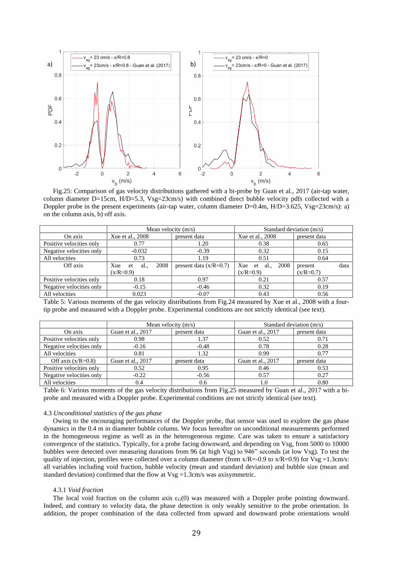
29
Fig.25: Comparison of gas velocity distributions gathered with a bi-probe by Guan et al., 2017 (air-tap water,
column diameter D=15cm, H/D=5.3, Vsg=23cm/s) with combined direct bubble velocity pdfs collected with a
Doppler probe in the present experiments (air-tap water, column diameter D=0.4m, H/D=3.625, Vsg=23cm/s): a)
on the column axis, b) off axis.
Mean velocity (m/s) Standard deviation (m/s)
On axis Xue et al., 2008 present data Xue et al., 2008 present data
Positive velocities only 0.77 1.20 0.38 0.65
Negative velocities only -0.032 -0.39 0.32 0.15
All velocities 0.73 1.19 0.51 0.64
Off axis Xue et al., 2008
(x/R=0.9)
present data (x/R=0.7) Xue et al., 2008
(x/R=0.9)
present data
(x/R=0.7)
Positive velocities only 0.18 0.97 0.21 0.57
Negative velocities only -0.15 -0.46 0.32 0.19
All velocities 0.023 -0.07 0.43 0.56
Table 5: Various moments of the gas velocity distributions from Fig.24 measured by Xue et al., 2008 with a four-
tip probe and measured with a Doppler probe. Experimental conditions are not strictly identical (see text).
Mean velocity (m/s) Standard deviation (m/s)
On axis Guan et al., 2017 present data Guan et al., 2017 present data
Positive velocities only 0.98 1.37 0.52 0.71
Negative velocities only -0.16 -0.48 0.78 0.28
All velocities 0.81 1.32 0.99 0.77
Off axis (x/R=0.8) Guan et al., 2017 present data Guan et al., 2017 present data
Positive velocities only 0.52 0.95 0.46 0.53
Negative velocities only -0.22 -0.56 0.57 0.27
All velocities 0.4 0.6 1.0 0.80
Table 6: Various moments of the gas velocity distributions from Fig.25 measured by Guan et al., 2017 with a bi-
probe and measured with a Doppler probe. Experimental conditions are not strictly identical (see text).
4.3 Unconditional statistics of the gas phase
Owing to the encouraging performances of the Doppler probe, that sensor was used to explore the gas phase
dynamics in the 0.4 m in diameter bubble column. We focus hereafter on unconditional measurements performed
in the homogeneous regime as well as in the heterogeneous regime. Care was taken to ensure a satisfactory
convergence of the statistics. Typically, for a probe facing downward, and depending on Vsg, from 5000 to 10000
bubbles were detected over measuring durations from 96 (at high Vsg) to 946” seconds (at low Vsg). To test the
quality of injection, profiles were collected over a column diameter (from x/R=-0.9 to x/R=0.9) for Vsg =1.3cm/s:
all variables including void fraction, bubble velocity (mean and standard deviation) and bubble size (mean and
standard deviation) confirmed that the flow at Vsg =1.3cm/s was axisymmetric.
4.3.1 Void fraction
The local void fraction on the column axis G(0) was measured with a Doppler probe pointing downward.
Indeed, and contrary to velocity data, the phase detection is only weakly sensitive to the probe orientation. In
addition, the proper combination of the data collected from upward and downward probe orientations would
a) b)

30
require to properly weight bubbles moving up and down. That weighting process would require the knowledge of
the phase detection error according to the orientation of the bubble velocity, an information we have not. This is
why only a downward oriented probe was considered for void fraction measurements.
The void fraction on the column axis G(0) happens to linearly increase with the height above injector for H/D
between about 1.5 up to 6, as shown Fig.26. Over that range of heights, the flow can be considered as quasi fully-
developed. Moreover, the slope dG/dH monotonously increases with Vsg (Fig. 26-right). Assuming an isothermal
system, with a constant bubble number density (no change due to coalescence and break-up), the axial change in
the void fraction induced by the bubble expansion due to the axial pressure gradient writes dG/dHhydrostatic = G (1-
G) Lg/P(H) where P(H) is the static pressure level at the measuring position. Assuming a hydrostatic pressure
gradient, dG/dHhydrostatic coincides with measurements of dG/dH in the homogeneous regime. On the opposite, in
the heterogeneous regime, dG/dHhydrostatic represents only 70% to 50% of the actual void fraction gradient. That
feature indicates that another mechanism is at play that controls the axial increase of the void fraction. A tentative
explanation could be that, among the bubbles that recirculate along the walls, some of them are captured by the
upward flow all along the column height. In other words, the upward two-phase flow in the central region of the
bubble column is continuously fed with a lateral gas flow rate all along the column height and not just at the
bottom the column.
Fig.26: Evolution of the local void fraction measured on the column axis G(0) with the height H above
injection (a), and evolution of the mean slope dG(0)/dH evaluated between H/D=1 and 6 versus the gas
superficial velocity compared with dG/dHhydrostatic (b). Measurements performed with a downward oriented
Doppler probe.
The evolution of the local void fraction G(0) measured on the column axis at H/D=3.625 with the superficial
velocity Vsg is provided Fig.27-a. According to that figure, the homogeneous regime ends up at Vsg about 4cm/s
in our conditions. Beside, in the heterogeneous regime (at Vsg=9cm/s), the transverse void fraction profiles
G(x/R) happen to be self-similar when normalized with G(0). That self-similarity holds (at least) from 2.6D
above the injector up to 4.87D (see Fig. 27-b). In addition, the normalized profiles compare well with the fit
proposed by Forret et al., 2006 that writes:
G(x/R) / G(0) = - 1.1927 [(x/R)6-1] + 0.8187 [(x/R)4-1] - 0.6260 [(x/R)2-1] (2)
b)a)

31
Fig.27: Local void fraction measured with a downward directed Doppler probe: a) evolution of the void
fraction on the column axis with the superficial velocity at H/D=3.625 and b) transverse void fraction profiles
normalized by the void fraction on the column axis measured at different heights above injection; comparison
with the fit (eq.(2)) proposed by Forret et al., 2006.
4.3.2 Bubble size
Let us first examine the bubble chords distributions detected by a downward directed Doppler probe when
considering direct velocity measurements only. As shown Fig.28-a, the chord pdf detected on the column axis and
in the heterogeneous regime does not vary with the height above injection when in the quasi-fully developed
region. That indicates that the size distribution was frozen in that region, that is either coalescence and break-up
were not active, or their contributions equilibrate in such a way that the size distribution was left unchanged in the
heterogeneous regime.
Then, by combining upward and downward orientations for the probe and using direct velocity measurements
only, let us then examine how the mean chord CG and its standard deviation CG’ evolve with the gas superficial
velocity. According to Fig.28-b and 28-c, both quantities steadily increase in the homogeneous regime, and they
both stabilize when in the heterogeneous regime. Indeed, the gas distributor has a fixed geometry so that the gas is
ejected through the orifices with a velocity that increases with Vsg: the latter ranges from a few m/s up to
≈100m/s at Vsg=25cm/s. At the end of the homogeneous regime, the gas ejection velocity is about 20m/s, and the
jet Reynolds number becomes of the order of ≈ 2000. This is roughly the onset of a turbulent jet. Hence, above the
homogenous/heterogeneous transition, the bubble size distribution is mainly controlled by the break-up of the
turbulent gas jets at injection, and that explains why it remains nearly the same in heterogeneous conditions.
These bubbles have a mean chord comprised between 4 and 4.5mm (Fig.28-b) with a standard deviation that is
about twice the mean (Fig.28-c).
In Fig.28-b and c, the mean chord and its standard deviation are also provided for a probe pointing downward
(data series “up flow”), for a probe pointing upward (data series “down flow”) and from the combined statistics (data series “up & down”). “Up flow” and “up & down” data almost coincide because of the very limited number
of velocity data collected on the column axis with a probe pointing upward (the velocity validation rate in that
case was at most 1.2%). Although limited, the data acquired with the probe pointing upward clearly indicate that
the bubbles moving downward are much smaller in size: their mean chord is about 2 to 2.5mm to be compared
with a mean chord about 4mm for bubbles moving up.
a) b)

32
Fig.28: a) Chord distributions on the column axis at various heights above injection using a downward directed
Doppler probe. Evolution with Vsg of the mean chord (b) and of the chord standard deviation (c) on the column
axis and at H/D=3.625: comparison between statistics for up flow, down flow and combined flow directions
(direct velocity measurements only).
Transverse profiles of the mean value CG aand of the standard deviation CG’ of chords are provided Fig.29.
The profiles of both CG and CG’ are nearly flat in the homogeneous regime (Fig.29-a). In the heterogeneous
regime, a limited radial segregation appears with a slight decrease of the mean chord at large x/R: typically, for
Vsg= 13cm/s and for Vsg=23cm/s; the chord decreases from ≈4mm in the center down to ≈3mm at x/R≈0.8
(Fig.29-b). In the mean time, the standard deviation decreases from ≈8mm in the center to 3-4mm at x/R≈0.8.
Fig.29-c compares mean values and standard deviations of chords between “up flow”, “down flow“ and “up &
down” data series. These data confirm the difference in the mean chord between bubbles moving up and bubbles
moving down. The standard deviation is also significantly larger (up to a ratio 2.5) for bubbles moving up
compared with those moving down. These differences persist when changing Vsg while staying in the
heterogeneous regime (not shown). Globally, the values from the “up flow” series are very similar to those from
the “up and down flow” series: they are slightly higher because of the limited proportion of downward moving
bubbles, a trend that holds up to x/R about 0.7-0.8.
Fig.29: Transverse distributions of the mean chord and of its standard deviation measured with a Doppler
probe: a) in the homogeneous regime at Vsg=1.3cm/s and 3cm/s from combined flow directions, b) in the
heterogeneous regime at Vsg= 13cm/s and 23cm/s from combined flow directions, (c) comparison between
moments for up flow, down flow and for combined flow directions at Vsg=23cm/s (direct velocity measurements
only). Measurements at H/D=3.625.
Finally, let us compare the size measured with the Doppler probe with alternate techniques. Table 7 provides
the Sauter mean vertical diameter measured with a single multimode optical probe using the dewetting time, as
well as the Sauter mean horizontal diameter measured with the correlation technique (Maximiano Raimundo et
al., 2016). From these data, we evaluate the mean eccentricity and the volume equivalent diameter Deq. From
the arithmetic mean chord CG measured with the Doppler probe, a Sauter mean vertical diameter is deduced
assuming spherical inclusions using Dv32=3CG/2. For ellipsoidal bubbles of the same eccentricity , that relation
becomes Dv32=(3/2) CG/ (Liu and Clark, 1995). We compare the Dv32 estimated from the Doppler probe with
Deq in the last two columns assuming either =1 or =0.85. If one except the data collected in the homogeneous
regime at Vsg=1.3cm/s (in this flow condition, the perturbation induced by the probe holder is quite significant),
the agreement between Dv32 and Deq is satisfactory (15-20% deviation) when assuming spherical bubbles (i.e.
=1). The agreement is even better (5% deviation) when considering a 0.85 eccentricity. In the present
experiments, the mean equivalent bubble diameter remains the same throughout the heterogeneous regime: it
a) b) c)
a) b) c)

33
equals 7mm±0.3mm. That size corresponds to distorted wobbling bubbles those terminal velocity UT in water and
under earth gravity is about 0.22cm/s: their particulate Reynolds number is about 1500.
Table 7: Comparison of mean bubble sizes measured with different techniques. Measurements taken on the axis at
H/D=3.625. For the Doppler technique, the mean chord CG provided here was obtained from direct velocity
measurements (no interpolation) from a downward directed probe.
4.3.3 Mean bubble velocity
Figure 30 provides the radial distributions of the mean vertical bubble velocity for two Vsg in the
homogeneous regime and for three Vsg in the heterogeneous regime. The data series indicated “up flow”
correspond to the mean vertical bubble velocity measured with a downward oriented probe only (and without
velocity interpolation). The mean bubble velocity indicated as “up & down” corresponds to the neat vertical
bubble velocity deduced by combining up and down probe orientations and by considering direct velocity
measurements only (no interpolation). By convention, a positive velocity is directed against gravity, and a
negative value is along gravity. The “up flow” and “up & down flow” velocity measurements are nearly the
same in the homogeneous regime. In the heterogeneous regime, they coincide well in the center of the column
where the flow is essentially upward directed, but they start to differ at x/R≥0.5: the difference between the two
increases with the distance to the axis because of the presence of stronger downward directed motions as one
approaches the wall as shown by the evolution of the bimodal pdfs in Fig.31.
Fig.30: Radial profiles of the upward vertical mean bubble velocity for various Vsg as measured from
combined (using up and down probe orientations) and direct (no interpolation) velocity measurements with the
Doppler probe (indicated as “up & down flow” in the legend). Comparison with the mean vertical bubble velocity
measured with a downward oriented probe only without interpolation (indicated as “up flow” in the legend).
Measurements in the D=0.4m bubble column at H/D=3.625.
vsg(m/s)
Meanchord
fromDoppler
probe(mm)
Dv(mm)measured
withaconical
probe
Dh(mm)measuredwith
correlation
technique
Deqdeduced
fromDvand
Dh(mm)
Meaneccentricity
c=Dv/Dh
Dv32estimatedfromDopplerprobewith
c=1/Deq
Dv32estimatedfromDopplerprobewith
c=0.85/Deq
0.013 2.51 6.66 6.6 6.62 1.01 0.58 0.690.065 3.65 6.69 6.82 6.77 0.98 0.81 0.95
0.13 3.97 6.47 7.35 7.05 0.88 0.84 0.99
0.163 4.0 6.22 7.59 7.1 0.82 0.85 0.990.195 4.0 6.59 7.76 7.35 0.85 0.82 0.97
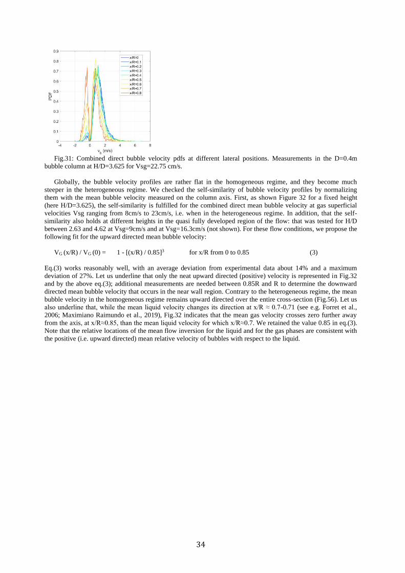
34
Fig.31: Combined direct bubble velocity pdfs at different lateral positions. Measurements in the D=0.4m
bubble column at H/D=3.625 for Vsg=22.75 cm/s.
Globally, the bubble velocity profiles are rather flat in the homogeneous regime, and they become much
steeper in the heterogeneous regime. We checked the self-similarity of bubble velocity profiles by normalizing
them with the mean bubble velocity measured on the column axis. First, as shown Figure 32 for a fixed height
(here H/D=3.625), the self-similarity is fulfilled for the combined direct mean bubble velocity at gas superficial
velocities Vsg ranging from 8cm/s to 23cm/s, i.e. when in the heterogeneous regime. In addition, that the self-
similarity also holds at different heights in the quasi fully developed region of the flow: that was tested for H/D
between 2.63 and 4.62 at Vsg=9cm/s and at Vsg=16.3cm/s (not shown). For these flow conditions, we propose the
following fit for the upward directed mean bubble velocity:
VG (x/R) / VG (0) = 1 - [(x/R) / 0.85]3 for x/R from 0 to 0.85 (3)
Eq.(3) works reasonably well, with an average deviation from experimental data about 14% and a maximum
deviation of 27%. Let us underline that only the neat upward directed (positive) velocity is represented in Fig.32
and by the above eq.(3); additional measurements are needed between 0.85R and R to determine the downward
directed mean bubble velocity that occurs in the near wall region. Contrary to the heterogeneous regime, the mean
bubble velocity in the homogeneous regime remains upward directed over the entire cross-section (Fig.56). Let us
also underline that, while the mean liquid velocity changes its direction at x/R ≈ 0.7-0.71 (see e.g. Forret et al.,
2006; Maximiano Raimundo et al., 2019), Fig.32 indicates that the mean gas velocity crosses zero further away
from the axis, at x/R≈0.85, than the mean liquid velocity for which x/R≈0.7. We retained the value 0.85 in eq.(3).
Note that the relative locations of the mean flow inversion for the liquid and for the gas phases are consistent with
the positive (i.e. upward directed) mean relative velocity of bubbles with respect to the liquid.

35
Fig.32: Radial profiles of the combined and direct mean bubble velocity scaled by the velocity on the axis
measured in the D=0.4m bubble column at H/D=3.625. Comparison with eq.(3). Comparison with the data
collected by Xue et al., 2008 with a four-tip probe at Vsg=30cm/s and H/D=8.5 in a D=0.162m diameter column.
Comparison with the data collected by Guan et al., 2017 with a bi-probe at Vsg=14cm/s and H/D=5.3 in a
D=0.15m diameter column.
It is interesting to compare the above findings with previous data, even though explorations of bubble velocity
in the near wall region are scarce.
• Yao et al., 1991 performed measurements at H/D=12 in a D=0.29m column (deionized water and air, ambient
conditions, no or weak coalescence, weak superficial liquid velocity of 1cm/s). With a five-point conductivity
probe, they measured up to x/R=0.82 and, at Vsg=8cm/s (i.e. in the heterogeneous regime), they detected
positive velocities only for the gas because they considered only one probe orientation. But, with the
ultrasound technique that is sensitive to the flow direction, they indeed measured a downward bubble velocity
at x/R=0.9 and for Vsg=8cm/s: this is in qualitative agreement with our results.
• Camarasa et al., 1999 measured gas velocity profiles with an ultrasonic probe in a D=0.1m column (tap water
and air, ambient conditions, possibly some coalescence) for a porous plate injector that delivers bubble from
1 to 10mm in diameter. The measuring height above injection is not precisely indicated but it seems to be
within the quasi-fully developed region. They observed negative gas velocities at x/R=0.75 in the
heterogeneous regime (at Vsg=8.4cm/s and 10.7cm/s) on one side of the column, but positive velocities up to
x/R=0.91 on the other side: clearly their mean flow was asymmetrical.

36
• Chen et al., 2003 in their 0.4m and 0.8 m diameter columns (tap water and air, ambient conditions, possibly
some coalescence) exploited the Doppler signal collected with a cleaved optical probe. Their measurements
were performed at H/D=2.6 for the 0.4 m column and at H/D=1.3 for the 0.8 m column: the latter condition is
possibly not within the quasi-fully developed region. As they successively used upward and downward
directed probes, negative bubble velocities were unambiguously detected. In the D=0.4 m column, the flow
was axisymmetric, and negative velocities were observed between x/R≈0.6 up to x/R≈0.8 and the wall: these
figures are comparable to our observations. A more quantitative comparison is not feasible, because the
authors have not estimated the mean bubble velocity from the data collected with the two probe orientations.
In the D=0.8 m column, Chen et al., 2003 observed downward motions between x/R≈0.4 up to x/R≈0.7 and
the wall. However, as shown by the profiles of bubble detection frequency, the flows in that column were
strongly asymmetrical (even at Vsg=3.3cm/s) and the authors attributed that to the presence of vortices at the
column scale: whatever the reason, such conditions are not comparable to ours.
• Xue et al., 2008 performed bubble velocity measurements in a D=0.162 column (tap water and air, ambient
conditions, probable significant coalescence) with a four-tip probe that was successively facing up and facing
down. Although they do not clearly indicate how a mean velocity was deduced from these two sets, they
consistently observed negative velocities (from ≈ -5 to -20cm/s) at x/R=0.9 on one side of the column when
in the heterogeneous regime (from Vsg=8 to 60cm/s). They also consistently observed positive velocities
(from ≈ 5 to 20cm/s) at x/R=0.9 on the other side of the column. Hence, and up to H/D≈5.1, all the
heterogeneous conditions they considered (that is for Vsg between 8 and 60cm/s) correspond to strongly
asymmetrical flows, a feature also confirmed by the void fraction profiles. At a larger distance from injection,
(H/D=8.5) they measured one gas velocity profile that proves to be more symmetrical, with a neat positive
velocity (≈ 50 cm/s) at x/R=0.6 and a neat negative velocity (between -10 and -20cm/s) at x/R≈0.88. These
last observations are consistent with ours. In addition, the gas velocity profile they obtained at H/D=8.5
compares well with our data and with the fit we propose (see Figure 32).
• Guan and Yang, 2017 performed measurements in a D=0.15 column (tap water and air, ambient conditions,
no or weak coalescence) with a horizontal dual conductivity probe. At H/D=5.3, they observed significant
positive bubble velocities (between 0.3 to 0.5m/s) up to x/R=0.8 (Fig.32). Yet, they do not detail their signal
processing, and it is unlikely that positive and negative velocities were distinguished by their measuring
system. Thus, without additional detail on the signal processing, the results they provide on the gas velocity
profiles in the near wall region should be taken with caution.
Overall, if one leaves aside the experiments in which asymmetrical flows were observed, literature results
available on bubble velocity profiles are in qualitative agreement with our measurements.
4.3.4 Standard deviation of the bubble velocity
Transverse profiles of the standard deviation VG’ of the bubble vertical velocity are given Figure 33 at various
gas superficial velocities. In the homogeneous regime (Vsg=1.3cm/s and 3cm/s), the profiles are flat over the
entire cross-section. Note that a weak contribution due to bubbles moving downward does exist at large x/R. Such
a contribution is probably due to some unsteadiness at injection because of gas maldistribution (Nedeltchev,
2020). An argument in favor of that scenario is that the downward contribution occurs only at very large x/R
(≥0.7) when the gas flow rate is low (Vsg=1.3cm/s), while it is already present at x/R≈0.4 for a larger gas flow
rate (Vsg=3cm/s).

37
Fig.33: Transverse profiles of the standard deviation VG’ of the bubble axial velocity estimated from combined
and direct measurements (data series indicated as “up & down flow”) and from direct measurements with a
downward directed probe only (data series indicated as “up flow”). Measurements with the Doppler probe in the
D=0.4m bubble column at H/D=3.625.
In the heterogeneous regime, the profiles of VG’ are similar at all the gas superficial velocities considered,
namely 13cm/s, 16cm/s and 22.75cm/s. The standard deviation VG’ relative to the downward motion (data series
“down flow” in Fig.33) is about 0.2 to 0.3 m/s: it is rather uniform. The standard deviation VG’ relative to the
upward motion (data series “up flow” in Fig.33) is larger (≈ 0.65 to 0.7m/s): it is maximum on the column center
and it decreases radially down to 0.4-0.5m/s. Finally, the standard deviation VG’ resulting from the combination of
up and down motions (data series “up & down flows” in Fig.33) increases slightly from 0.7 to 0.8 m/s with the
radial coordinate: that behavior is due to the increasing contribution of the downward oriented motion when
approaching the column wall (see also the velocity pdfs in Fig.31).
The standard deviation VG’ of the bubble vertical velocity on the column axis relative to the mean VG is
plotted versus Vsg in Figure 34: the statistics presented here are based on combined and direct velocity
measurements. For comparison, the quantity VL’/VL evaluated on the column axis is plotted in the same figure.
The mean VL and the standard deviation VL’ of the liquid phase velocity were deduced from Pavlov tube
measurements: these moments were evaluated considering the whole liquid velocity distribution (i.e. positive as
well as negative velocities, see Fig.22). Both VG’/VG and VL’/VL vary with the gas superficial in the homogeneous
regime. They both stabilize to nearly constant values in the heterogeneous regime: the velocity fluctuation relative
to the mean reaches 0.55 in the gas, to be compared with ≈0.36 for the liquid.
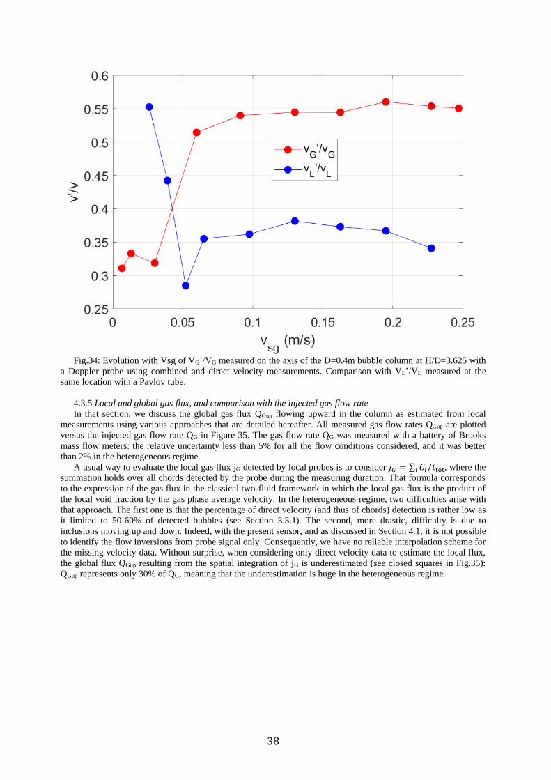
38
Fig.34: Evolution with Vsg of VG’/VG measured on the axis of the D=0.4m bubble column at H/D=3.625 with
a Doppler probe using combined and direct velocity measurements. Comparison with VL’/VL measured at the
same location with a Pavlov tube.
4.3.5 Local and global gas flux, and comparison with the injected gas flow rate
In that section, we discuss the global gas flux QGup flowing upward in the column as estimated from local
measurements using various approaches that are detailed hereafter. All measured gas flow rates QGup are plotted
versus the injected gas flow rate QG in Figure 35. The gas flow rate QG was measured with a battery of Brooks
mass flow meters: the relative uncertainty less than 5% for all the flow conditions considered, and it was better
than 2% in the heterogeneous regime.
A usual way to evaluate the local gas flux jG detected by local probes is to consider 𝑗𝐺 = ∑ 𝐶𝑖/𝑡tot𝑖 , where the
summation holds over all chords detected by the probe during the measuring duration. That formula corresponds
to the expression of the gas flux in the classical two-fluid framework in which the local gas flux is the product of
the local void fraction by the gas phase average velocity. In the heterogeneous regime, two difficulties arise with
that approach. The first one is that the percentage of direct velocity (and thus of chords) detection is rather low as
it limited to 50-60% of detected bubbles (see Section 3.3.1). The second, more drastic, difficulty is due to
inclusions moving up and down. Indeed, with the present sensor, and as discussed in Section 4.1, it is not possible
to identify the flow inversions from probe signal only. Consequently, we have no reliable interpolation scheme for
the missing velocity data. Without surprise, when considering only direct velocity data to estimate the local flux,
the global flux QGup resulting from the spatial integration of jG is underestimated (see closed squares in Fig.35):
QGup represents only 30% of QG, meaning that the underestimation is huge in the heterogeneous regime.

39
Fig.35: Upward gas flow rates deduced from the spatial integration of local fluxes measured at H/D=3.625
versus the injected gas flow rate. All data correspond to combined and direct velocity measurements. Local flux
are evaluated either using 𝑗𝐺 = ∑ 𝐶𝑖/𝑡tot𝑖 (squares) or using jG = G VG (dots and triangles). Dots correspond to
gas flow rates estimated using measurements on the column axis combined with eq.(4).
In order to circumvent the measuring difficulties related with changes in flow direction, we used a second
approach based on an alternate way to evaluate the local gas flux. Indeed, in the framework of hybrid models
inspired from kinetic theory, the dispersed phase is described by a product density f(1)(x, Db, Vb) where x refers to
the position of the center of the gas inclusion, and where internal coordinates include the bubble size Db, the
bubble velocity Vb, plus possibly other bubble characteristics such as their eccentricity, etc… In that framework,
the local gas flux is given by jG = G E[Vb Db3]/E[Db
3] where E[.] is the ensemble average over the phase space
(Cartellier, 1999). If bubble size and bubble velocity are not correlated, then jG = G E[Vb] where E[Vb] is the
mean bubble velocity. Because of the very strong agitation of the liquid-gas mixture due to the presence of meso-
scale structures (Maximiano Raimundo et al., 2019), bubble size and velocity are expected to be uncorrelated in
bubble columns especially when in the heterogeneous regime provided that coalescence remains weak or absent.
Besides, the mean bubble velocity E[Vb] is readily available from the Doppler probe as the arithmetic average VG
of bubble velocity measurements. The local void fraction required in the above formula is also available from the
Doppler probe. Therefore, the local gas flux can be evaluated as jG = G VG. The transverse profiles of the local
flux jG = G VG evaluated from the mean bubble velocity (Figure 32) and from the void fraction (Figure 27) are
shown Figure 36. As before, we focus on the upward flux, and we assume axisymmetric distributions for the
spatial integration. Data are lacking for x/R>0.8, but, according to mean bubble velocity profiles (see Fig.32), the
integration is stopped at x/R=0.85. The missing fraction of the upward flux for x/R between 0.8 and 0.85 has been

40
estimated using plausible assumptions: as it represents less than a few percent of the global flux, it has been
neglected. The global upward gas flow rates deduced from the integration of the transverse profiles are
represented by triangles in Figure 35.
Fig.36: Local flux profiles evaluated with jg = G VG, considering for the mean bubble velocity either
combined and direct measurements (data series indicated as “up & down flow”) or direct measurements with a
downward directed probe only (data series indicated as “up flow”). Measurements at H/D=3.625 in a D=0.4m
bubble column.
As a third approach, we considered the fits proposed in eq.(2) for the void fraction and in eq.(3) for the
positive mean axial bubble velocity valid for the heterogeneous regime. The integration over the cross section of
the product G VG using these fits provides a relationship between the global gas flow rate QGup flowing upward in
the column, and the values of the void fraction G(0) and of the mean, upward directed bubble velocity VG(0) on
the column axis in the heterogeneous regime. For that regime, we obtain:
QGup / (πR2) = 0.3735 G(0) VG(0) (4)
The global gas flow rates evaluated from eq.(4) and from the measured values of G(0) (Figure 27) and of VG(0)
(not shown) are represented in Figure 35 by closed dots.
Let us comment the results presented Figure 35. In the homogeneous regime (Vsg ≤ 5cm/s), the measured gas
flow rate QGup should equal the injected gas flow rate QG. According to Figure 35, the measured gas flow rate is
overestimated by at most 33%. A larger relative difference is observed at Vsg=3cm/s, but a maldistribution at
injection occurs at this superficial gas velocity (see Section 4.3.4), and that condition cannot be considered as
representative. To evaluate the sensor performance in terms of gas flux, more data with a better control of
injection need to be gathered in the homogeneous regime.
In the heterogeneous regime, the global recirculation of the liquid entrains a fraction of the gas from the top to
the bottom of the column. Therefore, the actual upward directed gas flow rate is expected to be larger than the
injected gas flow rate QG. In addition, and owing to the observed increase of the void fraction with the height
above injection (see Fig.26), the upward gas flow rate is also expected to increase with that distance. For these
reasons, there is no undisputable reference available for the upward gas flow rate. We attempted to estimate the
downward directed gas flow rate based on the experimental finding that the gas flux is directed downward for x/R
between 0.85 and 1 (see Fig.32) and using different approximations for the transverse gas velocity profile.
- First, we tentatively assumed that the eq.(3) proposed above remains valid up to the wall. This is not
demonstrated, but a couple of data from Xue et al., 2008 support that proposal (see Fig.32). Using that extended
eq.(3) and the void fraction provided by eq.(2), the integral of the local flux jG = G VG within the downward
directed zone represents 4.5% of the upward gas flow rate obtained by integrating between x/R=0 and 0.85.
- Second, assuming that the local bubble velocity VG equals VL plus a (constant) relative velocity UR, and
using the liquid velocity profile proposed by Forret et al., 2006, we compare the gas flow rate integrated between
41
x/R=0.85 and 1 to the gas flow rate integrated from the axis up to x/R=0.85. With UR set as the terminal velocity
(which is a fixed quantity, independent from Vsg in our flow conditions – see section 4.3.2), the recirculated gas
flow rate happens to represent between 1 and 4% of the upward gas flow rate. If one accounts for a swarm factor
those effect is to increase UR, these percentages would be even lower.
- Finally, if one us considers the crude limit in which UR is set to zero (i.e. no slip velocity), the recirculated
gas flow rate fraction reaches at most 20%.
To appreciate the validity of the above estimates, we tested whether the fits proposed by Forret et al., 2006 for the
liquid velocity and for the void fraction ensure equal upward and downward liquid fluxes. We found differences
ranging from 20% (at transition) to -20% (at large gas hold-up): these figures are typical of the reliability of the
proposed fits. Owing the various approximations considered above, it is difficult to unambiguously conclude on
the magnitude of the recirculated gas flow rate. Tentatively, the later seems comprised between a few percent and
20% of the upward gas flow rate. Knowing these magnitudes, and despite the associated uncertainties, let us now
comment on the difference between the measured upward global gas flux and the injected gas flow rate in the
heterogeneous regime. According to Figure 36, at moderate Vsg, the measured gas flow rate exceeds QG by at
most 18%. Above Vsg=13cm/s, the trend becomes opposite. Moreover, the difference monotonously increases
with Vsg, and it reaches -27% at the largest Vsg considered here (=24.7cm/s). Taking into account the unknown
contribution of the recirculation, these differences with the actual upward gas flow rate are probably larger. At this
stage, it is difficult to unambiguously identify the origin of the differences between QG and QGup. On one hand, the
perturbation induced by the thick probe holder used to limit vibrations is possibly significant in heterogeneous
conditions. On another hand, the characteristics of the global recirculation inside a bubble column are not known
with enough accuracy. In that perspective, it would be worth to closely scrutinize the near wall region using a
Doppler probe inserted in the flow through the wall to avoid vibration issues and to minimize the flow
perturbation occurring in these very low, and thus sensitive, velocity zones. At the present stage of the
investigation, we can nevertheless recommend to evaluate the upward directed gas flux based on jg = G VG, with
the void fraction measured with a downward oriented probe combined with a mean bubble velocity deduced from
the combination of direct velocity measurement for a probe pointing downward and then pointing upward. With
such an approach, one gets rid of the issue on data interpolation that is not solved for a flow that fluctuates between up and down motions.
5. Conclusions and perspectives
A new optical probe for size and velocity measurements of gas inclusions has been designed based on a single
mode optical fiber with an ad-hoc tip geometry. That probe combines the detection of incoming interfaces at a
high spatial resolution (its latency length is 6µm) with absolute velocity measurements from the analysis of
Doppler bursts occurring before gas-liquid transitions.
From the analysis of its optical response and from experiments in controlled conditions, we have shown that
the Doppler probe is sensitive to the trajectory of the incoming inclusion. More specifically, it only detects an
interface approaching the probe tip head-on, and those normal makes an angle with the fiber axis less than about
12-13°. That angular limit can be slightly changed by varying the number of oscillations and/or the threshold in
amplitude considered. Thanks to such sensitivity, the Doppler probe provides the translation velocity of the gas
inclusion projected along the fiber axis. The uncertainty on velocity measurement is less than 14%.
An optimized signal processing has been developed to extract variables of interest, namely gas arrival times,
gas residence times and velocities, from which one can infer statistics on velocity and size as well as
concentration, volumetric flux, number density, number density flux… The sensor and the processing were tested
in an air-water bubble column of diameter 0.4m and for superficial gas velocities between 1.3cm/s and 25cm/s.
No bias related with bubble size or with bubble acceleration was identified. The percentage of bubbles detected
for which a direct velocity measurement is available happens to be 66% in the homogeneous regime. That success
rate drops down to 50% in the strongly unsteady and three-dimensional flows encountered in the heterogeneous
regime. Yet, in these flow conditions, the mean bubble size measured with the Doppler probe was in agreement
with alternate techniques.
The sensor was exploited to gather new information on bubble motion in the heterogeneous regime. Over this
regime, the mean equivalent diameter remained constant, equal to 7mm±0.3mm, so that the corresponding particle
Reynolds number based on the terminal velocity was also fixed, equal to about 1500. As for the liquid, the
transverse profiles of the mean bubble velocity were found to be self-similar in the quasi-fully developed region
of the column. A fit is proposed for the upward directed mean bubble velocity: the latter reaches zero at a lateral
position x/R≈0.85. The transverse profiles of the standard deviation of the bubble velocity are nearly flat.
Meanwhile, on the column axis, the standard deviation of bubble velocity with respect to the mean increases with
the gas superficial velocity in the homogeneous regime, and it remains constant, equal to 0.55, in the entire
heterogeneous regime. This is significantly larger than the ratio 0.36 found for the liquid phase.
In terms of perspectives, future efforts should be devoted to a refined investigation of near wall zones to
quantify the recirculated gas flow rate as a function of flow parameters. To avoid the perturbation induced by the
large probe holder used in the present experiments, new data should be preferentially collected using a Doppler
42
probe inserted from the wall. Also, better resolved liquid velocity measurements are worth to be undertaken using
less invasive techniques. Finally, to better understand the hydrodynamics of bubble columns, the Doppler probe
opens the way to reliable bubble velocity measurements conditioned by the local concentration. Indeed, as the
existence of clusters and of void regions has been evidenced from a Voronoï analysis of the phase indicator
function delivered by optical probes (Maximiano Raimundo et al., 2019), information conditioned by the void
fraction are crucial to understand the hydrodynamics of bubble columns. One objective in particular is to relate the
swarm factor with the internal flow organization for given column size and injected gas flow rate.
CRediT authorship contribution statement
Anthony Lefebvre: Investigation, Methodology, Data curation, Writing - original draft
Yann Mezui: Investigation; Methodology, Data curation, Visualization
Martin Obligado: Investigation, Software, Data curation
Stéphane Gluck: Conceptualization , Investigation, Supervision
Alain Cartellier: Conceptualization, Investigation, Methodology, Roles/Writing - original draft; Writing - review
& editing, Supervision.
Declaration of Competing Interest
The authors declare that they have no known competing financial interests or personal relationships that could
have appeared to influence the work reported in this paper.
Acknowledgments
The LEGI is part of the LabEx Tec21 (Investissements d’Avenir - grant agreement n° ANR-11-LABX-0030).
That research was also partially funded by IDEX UGA (n° ANR-15-IDEX-0002).
Nomenclature
Abbreviations
ADC analog to digital converter
I.D. internal diameter
LDV Laser Doppler Velocimetry
pdf probability density function
RPP random Poisson process
0C cleaved tip
1C conical tip
3C conical-cylindrical-conical tip
1D one dimensional
3D three dimensional
Latin letters
a bubble radius, m
C chord cut through a bubble, m
Ci chord of the ith bubble, m
CG mean chord, m
CG’ standard deviation of chord pdf, m
CAM added mass coefficient, -
d fiber core diameter, m
dc probe tip size, m
dprobe probe diameter, m
D column diameter, m
Db bubble diameter, m
DRmeasured measured dynamic range, -
DRfilter dynamic range set by filters, -
DR0 actual dynamic range, -
f frequency, Hz
fD Doppler frequency, Hz
fk instantaneous frequency, Hz
fDmin minimum Doppler frequency, Hz
fDmax maximum Doppler frequency, Hz
fHP high pass frequency, Hz
fLP low pass frequency, Hz
fsampling sampling frequency, Hz

43
f0 light frequency in vacuum, Hz
fB bubble detection frequency, Hz
g gravitation acceleration, m/s2
H0 static liquid height, m
H height above injection, m
I, I1, I2 light intensities, W/m2
I0 light intensity at waist, W/m2
jG local gas flux, m/s
k unit vector along the light direction of propagation, -
L length, m
Ls latency length, m
LG cumulated gas length, m
n1, n2, next refractive indexes, -
neff effective group index, -
n number of Doppler periods, -
n vector normal to the interface, -
numerical aperture, -
Q flow rate, m3/s
r distance to the interface, m
Ra/b Fresnel coefficient at the frontier between media a and b, -
R column radius, m
t time, s
tA, tE characteristics times, s
TG, TGi gas residence time, gas residence time of the ith bubble, s
Ti date of the center of the ith bubble, s ttot total measuring duration, s
Tm de-wetting time, s
ub bubble velocity with respect to the probe, m/s
UT terminal velocity, m/s
V interface or reflector velocity, m/s
Vaxis interface displacement velocity projected along the probe axis, m/s
Vb, Vbi bubble velocity, velocity of the ith bubble, m/s
VG mean bubble velocity, m/s
VG’ standard deviation of bubble velocity pdf, m/s
Vmax maximum velocity detected, m/s
Vmin minimum velocity detected, m/s
Vsg gas superficial velocity, m/s
x radial coordinate, m
∆ti waiting time between successive direct bubble velocity measurements, s
<∆ti > mean waiting time, s
∆tcut threshold on the mean waiting time, s
∆tk Doppler period, s
Greek letters
inclination angle, rad
collection angle, rad
aspect ratio, -
relative difference between periods, %
G local void fraction, -
0 wavelength in vacuum, m
wavelength in medium, m
kinematic viscosity, m2/s
angle, rad
illumination angle, rad
eff effective illumination angle, rad
ρ density, kg/m3
surface tension, N/m
Dimensionless numbers
M modified Weber number, [ρL Db ub2/] (Db/dprobe)
44
Rep particulate Reynolds number, UT Db / L
Subscripts
D Doppler
G Gas phase
L liquid phase
______________________
References
Aliseda, A., Cartellier, A., Hainaux F., Lasheras, J.C., 2002, Effect of preferential concentration on the settling
velocity of heavy particles in homogeneous isotropic turbulence, J. Fluid Mech. 468, 77-105.
https://doi.org/10.1017/S0022112002001593
Barrau, E., Rivière, N., Poupot, Ch., Cartellier, A., 1999, Single and double optical probes in air-water two-phase
flows: real time signal processing and sensors performances. Int. J. Multiphase Flow, 25, 229-256.
https://doi.org/10.1016/S0301-9322(98)00042-1
Besagni, G., Inzoli, F., Ziegenhein, Th., 2018, Two-phase bubble columns: a comprehensive review,
ChemEngineering 2, 1-79. https://doi.org/10.3390/chemengineering2020013
Camarasa, E., Vial, C., Poncin, S., Wild, G., Midoux, N., Bouillard, J., 1999, Influence of coalescence behaviour
of the liquid and of gas sparging on hydrodynamics and bubble characteristics in a bubble column, Chem. Eng.
Process. 38, 329-344. https://doi.org/10.1016/S0255-2701(99)00024-0
Cartellier, A., 1990, Optical probes for local void fraction measurements: characterization of performances. Rev.
Sci. Instrum. 61(2), 874-886. https://doi.org/10.1063/1.1141457
Cartellier, A., 1992, Simultaneous void fraction measurement, bubble velocity and size estimate using a single
optical probe in gas-liquid two-phase flows. Rev. of Scientific Instruments 63, 11, 5442-5453.
https://doi.org/10.1063/1.1143416
Cartellier, A., 1998, Measurement of gas phase characteristics using new monofiber optical probes and real time
signal processing. Nuclear Engineering and Design, 184, 393-408. https://doi.org/10.1016/s0029-5493(98)00211-8
Cartellier, A., 1999, Post-treatment for phase detection probes in non-uniform two-phase flows, Int. J. Multiphase
Flow, 25, 201-228. https://doi.org/10.1016/S0301-9322(98)00041-X
Cartellier, A., 2001, Optical probes for multiphase flow characterization: Some recent improvements, Chemical
Engineering and Technology 24(5), 535-538. https://doi.org/10.1002/1521-4125(200105)24:5<535::AID-
CEAT535>3.0.CO;2-X
Cartellier, A., Achard, J.-L., 1985, Limitations of the classical LDA formula for velocity measurements for large
particles in two-phase suspension flows. Physico-Chemical Hydrodynamics 6(4), 481-563.
Cartellier, A., Achard, J.-L., 1991, Local phase detection probes in fluid/fluid two-phase flows. Review of
Scientific Instruments, 62(2), 279-303. https://doi.org/10.1063/1.1142117
Cartellier, A., Barrau, E., 1998a, Monofiber optical probes for gas detection and gas velocity measurements:
conical probes. Int. J. Multiphase Flow 24, 1265-1294. https://doi.org/10.1016/S0301-9322(98)00032-9
Cartellier, A., Barrau, E., 1998b, Monofiber optical probes for gas detection and gas velocity measurements:
optimized sensing tips. Int. J. Multiphase Flow 24, 1295-1315. https://doi.org/10.1016/S0301-9322(98)00033-
0
Chang, K.-A., Lim, H.J., Su, C.B., 2003, Fiber optic reflectometer for velocity and fraction ratio measurements in
multiphase flows, Rev. Sci. Instrum. 74(7), 3559-3565. https://doi.org/10.1063/1.1578152
Chaumat, H., Billet-Duquenne, A.M., Augier, F., Mathieu, C., Delmas, H., 2007, On the reliability of an optical
probe in bubble column under industrial relevant operating conditions, Exp. Therm. Fluid Sci. 31, 495–504.
https://doi.org/10.1016/j.expthermflusci.2006.04.018
Chen, R.C., Reese, J., Fan, L.-S., 1994, Flow structure in a three dimensional bubble column and three-phase
fluidized bed, AIChE J. 40(7), 1093-1104. https://doi.org/10.1002/aic.690400702
Chen W., Tsutsumi, A., Otawara, K., Shigaki, Y., 2003, Local bubble dynamics and macroscopic flow structure in
bubble columns with different scales, The Canadian Journal of Chemical Engineering 81, 1139-1148.
https://doi.org/10.1002/cjce.5450810603
Clift, R., Grace, J.R., Weber, M.E., 1978, Bubbles, Drops and Particles, Academic Press, New York.
Davoust, L., Achard, J.-L., Cartellier, A., 2000, Detection of waves at a contaminated interface by the way of an
optical fiber. Progress in Colloid and Polymer Science 115, 249-254. https://doi.org/10.1007/3-540-46545-
6_49
Deckwer, W., 1992, Bubble Column Reactors. Wiley, Chichester, New York.
De Nevers, N., 1968, Bubble driven flow circulation, AIChE J., 14(2), 222-226.

45
Do, J., Chuang, W.-L., Chang, K.-A., 2020, Oil droplet sizing and velocity determination using fiber-optic
reflectometer, Meas. Sci. Technol. 31, 065301. https://doi.org/10.1088/1361-6501/ab75b1
Durst, F., Melling, A., Whitelaw, J.H., 1976, Principles and practice of Laser-Doppler Anemometry, Academic
Press.
Ekambara, K., Dhotre, M.T., Joshi, J.B., 2005, CFD simulations of bubble column reactors: 1D, 2D and 3D
approach, Chem. Eng. Sci. 60(23), 6733-6746. https://doi.org/10.1016/j.ces.2005.05.047
Ferenc, F.S., Néda, Z., 2007, On the size distribution of Poisson Voronoi cells. Physica A: Stat. Mech. Appl. 385
(2), 518–526. https://doi.org/10.1016/j.physa.2007.07.063
Forret, A., Schweitzer, J.M., Gautier, T., Krishna, R., Schweich, D., 2006, Scale Up of Slurry Bubble Reactors,
Oil & Gas Science and Technology – Rev. IFP 61(3) 443-458. https://doi.org/10.2516/ogst:2006044a
Frijlink, J.J., 1987, Physical aspects of gassed suspension reactors, PhD thesis, Delft Technical University.
Gemello, L., Capello, V., Augier, F., Marchisio D., Plais, C., 2018, CFD-based scale-up of hydrodynamics and
mixing in bubble columns, Chem. Eng. Research and Design, 136, 846-858.
https://doi.org/10.1016/j.cherd.2018.06.026
Guan, X., Yang, N., 2017, Bubble properties measurement in bubble columns: From homogeneous to
heterogeneous regime, Chem. Eng. Research and Design 127, 103-112.
https://doi.org/10.1016/j.cherd.2017.09.017
Guet, S., Fortunati, R.V., Mudde, R.F., Ooms, G., 2003, Bubble velocity and size measurements with a four-point
optical fiber probe, Part. Part. Syst. Charact. 20, 219-230. https://doi.org/10.1002/ppsc.200390028
Harteveld, W.K., 2005, Bubble columns: Structures or stability? PhD thesis, Delft University of Technology,
ISBN 90-64642-26-5.
Hills, J.H., 1974, Radial non-uniformity of velocity and voidage in a bubble column, Trans. Instn. Chem. Engrs.
52, 1-9.
Hong, M., Cartellier, A., Hopfinger, E., 2004, Characterization of phase detection optical probes for the
measurement of the dispersed phase parameters in sprays. Int. J. Multiphase Flow 3, 615-648. https://doi.org/10.1016/j.ijmultiphaseflow.2004.04.004
Huck, P., Bateson, C., Volk, R., Cartellier, A., Bourgoin, M., Aliseda, A., 2018, The role of collective effects on
settling velocity enhancement for inertial particles in turbulence, J. Fluid Mech. 846, 1059-1075.
https://doi.org/10.1017/jfm.2018.272
Joshi, J.B., Parasu Veera, U., Prasad, Ch.V., Phanikumar, D.V., Deshphande, N.S, Thakre, S.S. and Thorat, B.N.,
1998, Gas hold-up structure in bubble column reactors, Proc. Indian National Science Academy 64 A n°4,
441-567.
Kantarci, N., Borak, F., Ulgen, K.O., 2005, Bubble column reactors, Process Biochemistry 40, 2263–2283.
https://doi.org/10.1016/j.procbio.2004.10.004
Kikukawa, K., 2017, Physical and transport properties governing bubble column operations, Int. J. Multiphase
Flow 93, 115-129. https://doi.org/10.1016/j.ijmultiphaseflow.2017.03.017
Liju, P.-Y., Machane, R., Cartellier, A., 2001, Surge effect during the water exit of an axisymmetric body
travelling normal to a plane interface: experiments and BEM simulation. Exp. in Fluids 31, 241-248.
https://doi.org/10.1007/s003480100277
Lim, H.-J., Chang, K.-A., Su, C.B., Chen, C.Y., 2008, Bubble velocity, diameter, and void fraction measurements
in a multiphase flow using fiber optic reflectometer, Rev. Sci. Instrum. 79, 125105.
https://doi.org/10.1063/1.3053271
Liu, W., Clark, N.N., 1995, Relationships between distributions of chord lengths and distributions of bubble sizes
including their statistical parameters, Int. J. Multiphase Flow 21(6), 1073-1089. https://doi.org/10.1016/0301-
9322(95)00039-Z
Maximiano Raimundo, P., 2015, Analyse et modélisation de l’hydrodynamique locale dans les colonnes à bulles,
Thèse de la Communauté Université Grenoble Alpes, Oct., 14 - in English.
Maximiano Raimundo, P., Cartellier, A., Beneventi, D., Forret, A., Augier, F., 2016, A new technique for in-situ
measurements of bubble characteristics in bubble columns operated in the heterogeneous regime, Chemical
Eng. Sc. 155, 504–523. https://doi.org/10.1016/j.ces.2016.08.041
Maximiano Raimundo, P., Cloupet, A., Cartellier, A., Beneventi, D., Augier F., 2019, Hydrodynamics and scale-
up of bubble columns in the heterogeneous regime: comparison of bubble size, gas holdup and liquid velocity
measured in 4 bubble columns from 0.15m to 3m in diameter, Chem. Eng. Sci. 198, 52-61.
https://doi.org/10.1016/j.ces.2018.12.043
McLure, D.D., Kavanagh, J. M., Fletcher, D. F., Barton, G. W., 2017 Experimental investigation into the drag
volume fraction correction term for gas-liquid bubbly flows, Chem. Eng. Sci. 170, 91-97.
https://doi.org/10.1016/j.ces.2016.12.066
Mezui M’Obiang Y., 2021, Hydrodynamique d'une colonne à bulle en régime hétérogène: Mécanismes, et
modélisation. Thèse de la Communauté Université Grenoble Alpes, June, 29 - in French.

46
Monchaux, R., Bourgoin, M., Cartellier, A., 2012, Analysing preferential concentration and clustering of inertial
particles in turbulence. Int. J. Multiphase Flow 40, 1-18.
https://doi.org/10.1016/j.ijmultiphaseflow.2011.12.001
Mora, D.O., Aliseda, A., Cartellier, A., Obligado, M., 2019, Pitfalls measuring 1D inertial particle clustering,
Springer Proceedings in Physics 226, 221-226. https://doi.org/10.1007/978-3-030-22196-6_35
Mudde, R.F., Saito, T., 2001 Hydrodynamical similarities between bubble column and bubbly pipe flow, J. Fluid
Mech. 437, 203-228. https://doi.org/10.1017/S0022112001004335
Nedeltchev. S., 2020, Precise identification of the end of the gas maldistribution in bubble columns equipped with
perforated plate gas distributors, Chem. Eng. J. 386 , 121535. https://doi.org/10.1016/j.cej.2019.04.115
Podkorytov, D.G., Timkin, L.S., Chinnov, Ye.A., 1989, Fiber-optics method for investigating boiling in cryogenic
fluids, Soviet J. of Applied Physics 3(3), 136-144.
Rollbusch, P., Bothe, M., Becker, M., Ludwig, M., Grünewald, M., Schlüter, M., Franke, R., 2015, Bubble
columns operated under industrially relevant conditions - Current understanding of design parameters, Chem.
Eng. Sci. 126, 660–678. https://doi.org/10.1016/j.ces.2014.11.061
Ruzicka, M.C., Zahradnik, J., Drahoš, J. and Thomas, N. H., 2001, Homogeneous–heterogeneous regime
transition in bubble columns, Chemical Engineering Science 56(15), 4609-4626.
https://doi.org/10.1016/S0009-2509(01)00116-6
Saito, T., Mudde, R.F., 2001, Performance of 4-tip optical fiber probe and bubble characterizations by the probe
in turbulent bubbly flows. In Proc. Fourth International Conference on Multiphase Flow, vol.27 n°111.
Sakamoto, A., Saito, T., 2012, Robust algorithms for quantifying noisy signals of optical fiber probes employed in
industrial-scale practical bubbly flows, Int. J. Multiphase Flow 41, 77-90.
https://doi.org/10.1016/j.ijmultiphaseflow.2011.12.004
Sekoguchi, K., Takeishi, M., Kano, H., Hironaga, K., Nishiura, T., 1984, Measurements of velocity and void
fraction in gas-liquid two-phase flow with an optical fiber, Proc. 2nd Int. Conf. on Laser Anemometry, paper
16.1, 2-4 July 1984, Lisbon, Portugal. Simonnet, M., Gentric, C., Olmos, E., Midoux, N., 2007, Experimental determination of the drag coefficient in a
swarm of bubbles, Chem. Eng. Sci. 62, 858-866. https://doi.org/10.1016/j.ces.2006.10.012
Sumbekova, S., Aliseda, A., Cartellier, A., Bourgoin, M., 2016, Clustering and settling of Inertial Particles in
Turbulence, in A. Segalini (ed.) Proceedings of the 5th International Conference on Jets, Wakes and Separated
Flows (ICJWSF2015), Springer Proceedings in Physics 185 (2016) 475-482. https://doi.org/10.1007/978-3-
319-30602-5_59
Uhlmann, M., 2020, Voronoï tessellation analysis of sets of randomly placed finite-size spheres, Physica A 555,
124618. https://doi.org/10.1016/j.physa.2020.124618
Vejrazka, J., Vecer, M., Orvalho, S., Sechet, Ph., Ruzicka, M., Cartellier, A., 2010, Measurement accuracy of a
monofiber optical probe in a bubbly flow, Int. J. Multiphase Flow 36 (2010) 533-548.
https://doi.org/10.1016/j.ijmultiphaseflow.2010.03.007
Wedin, R., Davoust, L., Cartellier, A., Byrne, P., 2003, Experiments and modeling on electrochemically generated
bubbly flows. Exp. Thermal and Fluid Sc. 27, 685-696. https://doi.org/10.1016/S0894-1777(03)00073-6
Wedin, R., Davoust, L., Cartellier, A., Dahlkild, A., 2000, A mono-modal fiber-optics velocimeter for
electrochemically-generated bubbles. paper 38-6, Proc. 10th Int. Symp. on Applications of Laser Techniques
to Fluid Mechanics, 10-13 July 2000, Lisbon, Portugal.
Xue, J., Al-Dahhan, M., Dudukovic, M.P., Mudde, R.F., 2003, Bubble dynamics measurements using four-point
optical probe, The Canadian Journal of Chemical Engineering 81, 375-381.
https://doi.org/10.1002/cjce.5450810306
Xue, J., Al-Dahhan, M., Dudukovic, M.P., Mudde, R.F., 2008, Bubble velocity, size, and interfacial area
measurements in a bubble column by four-point optical probe, AIChE J. 54(2), 350-363.
https://doi.org/10.1002/aic.11386
Yao, B.P., Zheng, C., Gasche, H.E., Hofmann, H., 1991, Bubble behavior and flow structure of bubble columns,
Chem. Eng. Process. 29, 65-75. https://doi.org/10.1016/0255-2701(91)87015-U
Recommended