A novel blind deconvolutionde-noising scheme in failureprognosisBin Zhang1, Taimoor Khawaja2, Romano Patrick1,George Vachtsevanos1,2, Marcos Orchard3 andAbhinav Saxena2
1Impact Technologies, LLC, Rochester, NY 14623, USA2School of Electrical and Computer Engineering, Georgia Institute of Technology,Atlanta, GA 30332, USA3Electrical Engineering Department, University of Chile, Av. Tupper 2007,Santiago, Chile
With increased system complexity, condition-based maintenance (CBM) becomes a promisingsolution for system safety by detecting faults and scheduling maintenance procedures beforefaults become severe failures resulting in catastrophic events. For CBM of many mechanicalsystems, fault diagnosis and failure prognosis based on vibration signal analysis are essentialtechniques. Noise originating from various sources, however, often corrupts vibration signalsand degrades the performance of diagnostic and prognostic routines, and consequently, theperformance of CBM. In this paper, a new de-noising structure is proposed and applied tovibration signals collected from a testbed of the main gearbox of a helicopter subjected to aseeded fault. The proposed structure integrates a blind deconvolution algorithm, featureextraction, failure prognosis and vibration modelling into a synergistic system, in which theblind deconvolution algorithm attempts to arrive at the true vibration signal through aniterative optimization process. Performance indexes associated with quality of the extractedfeatures and failure prognosis are addressed, before and after de-noising, for validationpurposes.
Key words: blind deconvolution; condition-based maintenance; de-noise; failure prognosis;
planetary gear carrier; vibration.
Address for correspondence: Bin Zhang, Impact Technologies, LLC, Rochester, NY 14623, USA.E-mail: [email protected] 2, 3 and 9–23 appear in colour online: http://tim.sagepub.com
Transactions of the Institute of Measurement and Control 32, 1 (2010) pp. 3–30
� 2010 The Institute of Measurement and Control 10.1177/0142331209357844

Nomenclature
f s Planetary carrier rotation frequencyNt Number of teeth in the annular gearp Index of gear in considerationNp Number of gearsm Index of harmonics of tooth meshing frequencyM Total number of tooth meshing harmonics in considerationN Index of harmonics of carrier rotation frequencyN Total number of carrier rotation harmonics in considerationD Angular phase shift caused by a crack on the plate�n Magnitude of modulating signal at its harmonic nf s
�m Magnitude of vibration signal from a single gear at its harmonic mNtfsup,m,n Magnitude of frequency components from gear p at sideband mNtþnG Remainder of (mNtþ n)/Np
lm,n Magnitude of combined vibration signal (superposition of vibration signals fromdifferent gears) at sideband mNtþ n
�� Angular phase evenly separated by Np gearsWm,n Weighting factor of non-linear projection at sideband mNtþ n�p Angular position of gear p
1. Introduction
The increasing demand for system safety and reliability requires that faults in complexdynamic systems be detected and isolated as early as possible so that maintenancepractices can be scheduled before faults become severe. Traditional breakdown andscheduled maintenance practices are, therefore, replaced by condition-based mainte-nance (CBM) to meet this need (Vachtsevanos et al., 2006). CBM is an integration ofsignal processing, feature extraction, fault detection and isolation, failure prognosis,and decision-making. In order to implement CBM, the health of critical componentsand subsystems must be monitored and reliable diagnostic/prognostic strategiesdeveloped (Vachtsevanos et al., 2006). Then, the system health can be assessed andmaintenance practices can be scheduled based on the remaining useful life ofcomponents/systems to avoid catastrophic events.
Performance of failure prognostic routines, however, is closely related to thefeatures (also known as condition indicators) derived from sensor data, which revealthe evolution and propagation of a failure in the system (Lebold et al., 2000; Saxenaet al., 2005; Wu et al., 2004, 2005). For many mechanical systems, features are typicallyextracted from vibration data (Keller and Grabill, 2003). During the operation of sucha system, if a fault occurs, it is expected that the vibration signals will exhibit acharacteristic signature, which reveals the severity and location of the fault. Noise inthe system, however, often corrupts the vibration signals and masks the indication offaults, especially in their early stages, thus curtailing the ability to diagnose andpredict failures accurately. Therefore, it is important to develop a good and reliable
4 Novel blind deconvolution de-noising scheme

de-noising scheme to improve the signal-to-noise ratio and make the characteristics ofthe fault perceptible in the vibration data. This process will improve the quality of theobtained features, potentially lower the fault detection threshold while increasing theaccuracy of the diagnostic and prognostic algorithms.
The main transmission of Blackhawk and Seahawk helicopters employs afive-planet epicyclic gear system, which is a critical component directly related tothe availability and safety of the vehicle (Keller and Grabill, 2003; McFadden andSmith, 1985). Recently, a crack in the planetary carrier plate was discovered duringregular maintenance, as shown in Figure 1. This resulted in major overhaul, re-designand replacement of gear plates with a high cost associated with these activities.Manual inspection of all transmissions is not only costly, but also time prohibitive(Saxena et al., 2005). CBM could provide a cost-effective solution for reducing the workburden and enhancing vehicle safety (Saxena et al., 2005). Many research effortstowards designing and implementing CBM on helicopters, such as vibration signalpreprocessing (Szczepanik, 1989; Wu et al., 2004), vibration signal modelling (Patrick,2006), features extraction (Wu et al., 2004, 2005), detection of cracks, and prediction ofcrack length (Orchard, 2006), have been carried out. The objective of this paper is topropose a new vibration pre-processing structure, which synergizes vibrationde-noising, vibration modelling, feature extraction and failure prognosis, to enhancethe performance of CBM. The planetary gear system with a seeded crack on the gearcarrier plate will be used to verify the proposed method.
For an epicyclic gear system, the widely used de-noising technique is timesynchronous averaging (TSA), which can be implemented in the time or frequency
Figure 1 The crack of planetary gear carrier plate of the UH-60Ahelicopter
Zhang et al. 5

domain (Keller and Grabill, 2003; Lebold et al., 2000; Szczepanik, 1989; Wu et al., 2004,2005). This operation enhances the components at the frequencies that are multiples ofthe shaft frequency, which are often related to the meshing of gear teeth (Wu et al.,2004, 2005). At the same time, it tends to average out external random disturbancesand noise that are asynchronous with the rotation of the gear.
Other de-noising algorithms include blind source separation (BSS; Antoni, 2005;Ayers and Dainty, 1988; Gelle et al., 2000), stochastic resonance (Klamecki, 2005), andadaptive schemes (Antoni and Randall, 2004; Hillerstrom, 1996). BSS aims to extractindividual, but physically different, excitation sources from the combined outputmeasurement (Antoni, 2005). Because of the complex environment and the largenumber of noise sources in mechanical systems, the application of BSS is severelyhindered (Antoni, 2005). A practical solution is to focus on the main vibration sourcethat contributes mostly to the vibration, while it treats all other sources as a combinednoise. Then, the objective is reduced to separating the vibration source from noise,which, in this sense, is the cumulative contribution of many different sources. Thisleads to a blind deconvolution de-noising algorithm (Kundur and Hatzinakos, 1998;Nandi et al., 1997; Peled and Braun, 2005).
Previous research work reported in Patrick (2006) has provided a good under-standing of the true vibration signals, originating from the epicyclic gearbox underboth healthy and faulty operational conditions. However, little knowledge about thenoise profile is available. To remove noise and recover the actual vibration signal, ablind deconvolution algorithm developed for a similarly formulated image-processingproblem (Kundur and Hatzinakos, 1998) will be modified and employed. The paperaddresses in detail the structure of the overall de-noising scheme, the analysis ofvibration mechanisms, the blind deconvolution algorithm, as well as its experimentalverification. The results show that the proposed de-noising scheme can substantiallyimprove the signal-to-noise ratio, feature performance and the precision of the failureprognostic algorithm.
2. The de-noising scheme architecture
The proposed overall de-noising scheme is illustrated in Figure 2. An accelerometermounted on the gearbox frame collects vibration signals and the TSA signal s(t) iscalculated. The blind deconvolution de-noising algorithm is carried out in thefrequency domain, and hence s(t) is Fourier transformed to arrive at S(f). Then, thede-noising algorithm is applied to S(f), which outputs the de-noised vibration data inthe frequency domain B(f). If the time domain signal is required, B(f) can be inverseFourier transformed to obtain b(t). From B(f) and b(t), features can be extracted andfused to be used subsequently for fault diagnosis and failure prognosis. With the mainobjective being remaining useful life prediction, the failure prognosis algorithm alsoprovides an estimate of crack length on the planet gear carrier plate as a function of
6 Novel blind deconvolution de-noising scheme

time (Orchard, 2006). Both the estimated crack length and load profile of the helicopter
serve as inputs to the vibration model (Patrick, 2006), which generates the noise-free
modelled vibration signal m(t). This modelled vibration signal is Fourier transformed
into the frequency domain and its frequency spectra are normalized to obtain the
weighting factor vector W(f), which is used in a non-linear projection of the blinddeconvolution de-noising algorithm.
The architecture of the proposed de-noising algorithm is decomposed and shown in
Figure 3. In this scheme, a non-linear projection, which is based on vibration analysis
in the frequency domain, and a cost function minimization are critical components,which are described in the sequel. Initially, an inverse filter �Zð f Þmust be defined. This
inverse filter is an initial estimate of the modulating signal in the frequency domain,
and converges to a filter through an optimization routine that recovers the vibration
signal from the noisy measured data S(f). The initial inverse filter �Zð f Þ is convoluted
S(f )
W (f )
Bnl(f )
E(f )
B(f )
Weighting factor
Nonlinear projection
Cost functionminimization
YNOK ?
+
–
Figure 3 Blind deconvolution de-noising scheme
100%80%
40%20%
FFTBlind
Deconvolution Feature
Extraction/Fusion Diagnosis/Prognosis
Vibrationmodel
TSA data
S(t )
S(f )
W(f )
B(f )
b(t )
m(t )
Estimated crack length
Load profile
Weightingfactor
IFFT
Remaininguseful lifeestimate
Figure 2 The overall structure of the de-noising scheme
Zhang et al. 7

with S(f) to obtain a rough estimate of the noise-free vibration signal �Bð f Þ. The signal�Bð f Þ passes through the non-linear projection, which maps �Bð f Þ to a subspace thatcontains only known characteristics of the vibration signal, to yield Bnl(f). Thedifference between �Bð f Þ and Bnl(f) is denoted as E(f). By adjusting �Zð f Þ iteratively tominimize E(f), and when E(f) reaches a minimal value, the signal �Bð f Þ!B(f) can beregarded as the de-noised vibration signal. At the same time, �Zð f Þ converges to Z(f).Through an inverse Fourier transform, the de-noised vibration signal in the timedomain can be obtained as well.
3. Vibration data analysis
The vibration signals are derived from the main transmission gearbox of Blackhawkand Seahawk Helicopters. The gearbox is an epicyclic gear system with five planetgears, the configuration of which is illustrated in Figure 4. The gearbox is mounted ona test cell, with a seeded crack fault on the planetary gear carrier. The followingsections intend to describe the expected vibration data in the healthy and faulty gearcarrier plate, respectively.
3.1 Healthy gearbox
Let us assume that the gearbox is an ideal healthy system without cracks. Theaccelerometer is mounted at a fixed point at position �¼ 0. Since the vibration signal is
Vibrationsensor
Annulusgear
q1=0
p =1
p =2
p =3 p =...
qp=...
p =Np
Planetgear
Planetarycarrier
=NpNumber
of planets
Sungear
q2= 2πNp
q3= 4πNp
Figure 4 The configuration of an epicyclic gear system
8 Novel blind deconvolution de-noising scheme

generated from the meshing of gear teeth and the planetary gears are rotating inside
the angular gear, the vibration signal is amplitude-modulated to the static
accelerometer. That is, the observed vibration amplitude will be large when the
planetary gear is close to the accelerometer and it will be small when the planetary
gear is far. Suppose that there is only one planetary gear, then the vibration observed
by the transducer should have the largest amplitude when the planetary gear is at�¼ 0, 2p, 4p, . . . . Similarly, the vibration should have the smallest amplitude at �¼ p,
3p, 5p, . . . . Suppose that the planetary carrier has a rotation frequency f s. The vibration
amplitude-modulating signal for this single planet gear and its spectra, which show
components at harmonics of f s, are illustrated in Figures 5(a) and (b), respectively. In
Figure 5(b), n is the index of harmonics of f s and �n is the amplitude of the component
of the modulating signal at frequency n f s.In the ideal case, the Np¼ 5 planetary gears are evenly spaced. Then, the planetary
gear p at time instant t has a phase:
�p ¼ 2� fstþp� 1
Np
� �ð1Þ
The amplitude-modulating signal for planetary gear p can be written in the time
domain as:
apðtÞ ¼XN
n¼�N
�n cos n�p
� �ð2Þ
where N is the number of sidebands about the harmonics under consideration.In this case, it is natural to assume that all mesh vibrations generated from different
planetary gears are of the same amplitude but of different phase shifts. The annulus
gear has Nt¼ 228 teeth. Since the speed at which teeth meshing is proportional to the
angular velocity of the planetary carrier, the meshing vibration appears at frequencies
Ntfs (McFadden and Smith, 1985; Patrick, 2006). In addition, supposing that, in the
frequency domain, the meshing vibration signal has amplitudes of �m at its harmonics
Amplitude
–π 0
Amplitude
0
n=0 1 2 3 4 ...
(a) (b)
π
α1α2 α3
α4
α0
f s 2f s 3f s 4f s f
Figure 5 Vibration amplitude modulation signal: (a) time domainmodulating signal; (b) frequency domain modulating signal
Zhang et al. 9

mNtfs, the spectra are illustrated in Figure 6. Then, the vibration signal generated from
planet gear p can be written in the form of:
bpðtÞ ¼XMm¼1
�m sin mNt�p
� �ð3Þ
where M is the number of harmonics under consideration.The observed vibration signal of planetary gear p, with respect to the static
accelerometer, is given as the product of the meshing vibration signal and the
amplitude-modulating signal. It is denoted as yp(t), with frequency spectra as shown
in Figure 7, and is given by:
ypðtÞ ¼ apðtÞbpðtÞ ¼1
2
XMm¼1
XN
n¼�N
�n�m sin ðmNt þ nÞ�p
� �ð4Þ
Amplitude
0 Ntf s 2Ntf s 3Ntf s
½α3b1
½α2b1
½α1b1
½α3b2 ½α3b3½α2b3
½α1b3
½α2b2
½α1b2α0b1
α0b2
α0b3
... ... ......
–3 –2 –1 0 1 2 3 –3 –2 –1 0 1 2 3 –3 –2 –1 0 1 2 3
m=
n=
f
1 2 3
Figure 7 Vibration spectrum of a single planet
0
m= 1 2
Amplitude
3 4 ...
b1
b2
b3b4
Ntfs 2Ntf
s 3Ntfs 4Ntf
s f
Figure 6 Spectrum of tooth meshing vibration of a singleplanet gear
10 Novel blind deconvolution de-noising scheme

Note the sidebands around the meshing vibration harmonics, compared withFigure 6. The ‘sidebands’ are defined as the frequency components that appear as a
harmonically spaced series (McFadden and Smith, 1985; Patrick, 2006). The position of
the sidebands can be located by mNtþ n or (m, n) with m being the index of meshing
vibration harmonics and n the index of the modulating signal harmonics.When there are more than one, say Np, planetary gears, the vibration signal observed
by the accelerometer is the superposition of the Np vibration signals generated from
Np different planetary gears. This superposition vibration signal has the form:
yðtÞ ¼1
2
XNp
p¼1
XMm¼1
XN
n¼�N
�n�m sin ðmNt þ nÞ�p
� �
¼1
2
XNp
p¼1
XMm¼1
XN
n¼�N
�n�m sin 2�ð p� 1ÞmNt þ n
Np
� �ð5Þ
where Equation (1) and the fact that sin(2kpþ �)¼ sin(�) for any integer k are used.Since the planetary gears are evenly spaced, the phase angle of the sidebands will
be evenly spaced along 2p (McFadden and Smith, 1985). From Equation (5), it is
obvious that if sideband mNtþ n is not a multiple of Np and (mNtþ n)/Np has a
remainder of g, the vibration components from different gears are evenly spaced by an
angle 2gp/Np. In this case, when the vibrations generated from different planetarygears are combined, these sidebands add destructively and become zero as illustrated
in Figure 8(a), in which up,m,n with 1� p� 5 indicates the frequency components of
gear p. Those frequency components appear at sidebands where mNtþ n 6¼ kNp are
termed non-regular meshing components (NonRMC).Conversely, if sideband mNtþ n is a multiple of Np, the remainder of (mNtþ n)/Np
will be zero. In this case, the vibration components from different gears do not have a
j 2,m,n
j 1,m,n
j 1,m,n
j 2,m,n
j 3,m,n
j 4,m,n
j 5,m,n
∑pj p,m,n=0
∑pj p,m,n= 5j1,m,n
j 3,m,n
j 5,m,nj 4,m,n
2hpNp
(a) (b)
Figure 8 Examples of superposition of vibration signal fora healthy gear plate with Np¼ 5: (a) mNtþ n 6¼ kNp (NonRMC);(b) mNtþ n¼ kNp (RMC)
Zhang et al. 11

phase difference. When the vibration signals from different planetary gears arecombined, these sidebands add constructively and are reinforced as illustrated in
Figure 8(b). These frequency components that appear at sidebands where
mNtþ n¼ kNp are referred to as regular meshing components (RMC) or apparent
sidebands.This process of frequency components adding destructively/constructively finally
generates asymmetrical sidebands. Partial frequency spectra of the sidebands around
the first-order harmonic that illustrates this asymmetry are shown in Figure 9, where
Np¼ 5 and Nt¼ 228. Note that the peak of the spectrum does not appear at n¼ 0 (order
228) but at n¼�3 (order 225), n¼ 2 (order 230), etc. The largest spectral amplitude
(also known as dominant sideband) appears at the frequency closest to the gearmeshing frequency (Keller and Grabill, 2003).
According to the above vibration analysis in the frequency domain and previ-
ous research results (Keller and Grabill, 2003; McFadden and Smith, 1985;
Patrick, 2006), for an ideal system, only terms at frequencies that are multiples ofthe number of planetary gears (ie, RMC) survive, whereas the terms at other
frequencies (ie, NonRMC) vanish. Then, the Fourier transform of the vibration data
can be written as:
Yð f Þ ¼ fhea lm,n ðmNt þ nÞ f s� �� �
ð6Þ
where lm,n is the magnitude of the spectral amplitude at (mNtþ n)f s and fhea is the
non-linear projection for an ideal healthy gearbox given by:
fhea ¼1 if mNt þ n is a multiple of Np
0 otherwise
�ð7Þ
215 220 225 230 235 240–0.1
0
0.1
0.2
0.3
0.4
Frequency (order of fs)
Am
plitu
de
Figure 9 Vibration spectrum of combined signal with Nt¼ 228and Np¼ 5
12 Novel blind deconvolution de-noising scheme

3.2 Faulty gearbox
When there is a crack on the planetary gear carrier, as in Figure 1, the five gears will
not be evenly separated along 2p. Suppose that, at time instant t, one of the fiveplanetary gears has an angle shift � caused by the crack. Then, this planetary gear has
a phase of �pþ � at time instant t with �p being given in Equation (1). For this gear, the
modulating signal becomes:
a0p ¼XN
n¼�N
�n cos nð�p þ �Þ� �
ð8Þ
The vibration signal generated from this gear is:
b0p ¼XMm¼1
�m sin mNtð�p þ �Þ� �
ð9Þ
Accordingly, the modulated vibration signal from this gear is written as:
y0pðtÞ ¼ a0pðtÞb0pðtÞ ¼
1
2
XMm¼1
XN
n¼�N
�n�m sin ðmNt þ nÞð�p þ �Þ� �
ð10Þ
If we denote by ��¼ 2p(p-1)/Np, then when the vibration signals from the five planetary
gears are superposed (note that the other four gears do not have a phase shift), the
observed vibration signal should have the form of (suppose the phase shift happens
on the last gear):
y0ðtÞ ¼1
2
XNp�1
p¼1
XMm¼1
XN
n¼�N
�n�m sin ðmNt þ nÞ�p
� �þ
1
2
XMm¼1
XN
n¼�N
�n�m sin ðmNt þ nÞð�p þ �Þ� �
¼1
2
XMm¼1
XN
n¼�N
�n�m
XNp�1
p¼1
�n�m sin ðmNt þ nÞ ��� �
þ sin ðmNtþ nÞð �� þ �Þ� � !
ð11Þ
Because of this phase shift, when mNtþ n is not a multiple of Np, the vibration
components from different gears are not evenly spaced. This can be illustrated in
Figure 10(a). It is obvious that the vibration components are not cancelled in this case.
This results in higher NonRMC frequency components. On the other hand, whenmNtþ n is a multiple of Np, the vibration components from different gears are not
exactly in phase. The vibration component from the last gear has a phase difference,
which results in lower RMC frequency components, as shown in Figure 10(b).To see this effect in real vibration signals, the frequency spectra around the first
harmonic for two different crack sizes at 1.35 inches and 4.4 inches are shown in
Figure 11. The components in the circles are the NonRMC. This is consistent with the
Zhang et al. 13

analysis in Figure 10(a). When (mNtþ n)� changes from 0 to p, the NonRMC changesfrom a minimum to a maximum amplitude, whereas the RMC from a maximum to aminimum. On the other hand, when (mNtþ n)� changes from p to 2p, the NonRMCbecomes from a maximum amplitude to a minimum, whereas the RMC from aminimum to a maximum.
Then, it is clear that the non-linear projection, given in (7), under the assumption ofa healthy gearbox, is not suitable for a faulty one. A reasonable modification of thenon-linear projection is given as follows. From previous research in Patrick (2006), avibration model in the frequency domain is established with the load profile and thecrack size being two of the inputs. Note that the load profile is known and the cracksize can be estimated from the prognostic algorithm (Orchard, 2006). Then, themodelled noise-free vibration signal m(t) generated from the vibration model is
220 225 230 235 2400
0.4
0.8
Frequency (order of fs)
Am
plitu
de
Small crackLarge crack
NonRMC
RMCNonRMC
NonRMCNonRMC
RMC
RMC
RMC
Figure 11 The influence of crack size on frequency spectra
j 2,m,n
j 1,m,n
j 1,m,n
j 2,m,n
j 3,m,n
j 4,m,n
∑pjp,m,n(crack)
∑pj p,m,n(no crack)
∑pj p,m,n(crack)∑pj p,m,n=(no crack)
j 3,m,n
j 5,m,n
(mNt + n) d
(mNt + n)j 5,m,n
j 4,m,n
2hpNp
2gpNp
(a) (b)
Figure 10 Examples of superposition of vibration signal fora faulty gear plate with Np¼ 5: (a) mNtþ n 6¼ kNp (NonRMC);(b) mNtþ n¼ kNp (RMC)
14 Novel blind deconvolution de-noising scheme

Fourier transformed in the frequency domain to arrive at M(f). The magnitude of M(f)is normalized to obtain weighting factors W(f). For illustration purposes, a modelsignal m(t) and the weighting factor W(f) derived from its frequency spectra are shownin Figures 12(a) and 12(b). The weighting factors around the first harmonic arezoomed in Figure 12(c).
When a frequency domain signal �Bð f Þ is fed into the non-linear projection, itsfrequency components are multiplied by the weighting factor W(f) to arrive at theoutput of the non-linear projection Bnl(f). Suppose that, for a sideband located at(mNtþ n) f s, �Bð f Þ has a magnitude of lm,n, then, after the non-linear projection, themagnitude of Bnl(f) at this sideband is given by Wm,n(f)lm,n, where Wm,n(f) is theweighting factor at sideband mNtþ n. It is clear that the non-linear projection in thiscase is:
fnl ¼Wm,nð f Þ 8 ðmNt þ nÞ 2 Dsup ð12Þ
Note that the non-linear projection under the healthy gearbox case in Equation (7) is aspecial case of (12).
From the above analysis of the system vibration behaviour, the followingassumptions are made and used in the blind deconvolution de-noising scheme:
(1) The majority of vibration information is contained in limited number of sidebandsaround the harmonics, which form the Dsup. Note that the frequency spectra fadequickly on both sides of the harmonics; this assumption is reasonable consideringsubsequent results.
(2) The non-linear projection that maps a signal into a subspace contains only knowncharacteristics of the vibration signal is given in (12).
(3) The amplitude of the modulating signal a(t) decreases monotonically on either side ofits maximum value until it reaches the minimum. Note that this assumption issomewhat restrictive.
0 0.5 1 1.5 2 ×10⁴–3
–2
–1
0
1
2
3(a) (b) (c)
Time
Am
plitu
de
0 500 1000 15000
0.10.20.30.40.50.60.70.80.9
1
Frequency (order of f s) Frequency (order of f s)
Am
plitu
de
215 220 225 230 235 240 2450
0.1
Am
plitu
de
Figure 12 The model vibration signal and weighting factor:(a) the model vibration signal with crack; (b) the weighting factor,normalized model vibration spectra; (c) the weighting factor atthe first harmonic
Zhang et al. 15

4. Blind deconvolution de-noising scheme
From the vibration analysis of the gearbox, we know that the vibration signalscollected from the transducer are amplitude modulated (McFadden and Smith, 1985;Patrick, 2006). Multiple sources of noise may further corrupt the signal. A simplifiedmodel for such a complex signal may be defined as:
sðtÞ ¼ aðtÞbðtÞ þ nðtÞ ð13Þ
where s(t) is the noisy vibration signal, b(t) is the noise-free unmodulated vibrationsignal, a(t) is the modulating signal and n(t) is the cumulative additive noise.
Note that the modulating signal a(t) is itself affected by noise in the system. Let aðtÞdenote the ideal or noise-free modulating signal and na(t) the noise introduced in thissignal. Consequently, a(t) can be represented as:
aðtÞ ¼ aðtÞ þ naðtÞ ð14Þ
Thus, Equation (13) can be rewritten as follows:
sðtÞ ¼ aðtÞ þ naðtÞð ÞbðtÞ þ nðtÞ
¼ aðtÞbðtÞ þ nðtÞð15Þ
where nðtÞ ¼ na(t)b(t)þ n(t) contains the total additive noise in the system. On the otherhand, the factor aðtÞ describes the multiplicative noise in the system. The goal for ade-noising scheme, such as the one described here, is to recover the unknownvibration signal b(t) from the observed signal s(t), given partial information about thenoise sources and characteristics of the vibration signal.
A typical approach would be to find the inverse of aðtÞ,
zðtÞ ¼ 1=aðtÞ ð16Þ
such that
bðtÞ ¼ ðsðtÞ � nðtÞÞ � zðtÞ
¼ sðtÞzðtÞ � nðtÞzðtÞð17Þ
Note, however, that little can be assumed about nðtÞ and aðtÞ is not available; zðtÞ is notapplicable. To solve this problem, rather than using zðtÞ, we propose an iterativede-noising scheme that starts with �zðtÞ, a very rough initial estimate of the inverse ofthe modulating signal, which demodulates the observed signal s(t) to give a roughnoise-free vibration signal:
�bðtÞ ¼ sðtÞ � �zðtÞ ð18Þ
If partial knowledge about how the plate system is influenced by the modulatingsignal aðtÞ and a reasonable understanding of the true vibration signal is available,then the ideal characteristics of the vibration signal can be obtained by projecting this
16 Novel blind deconvolution de-noising scheme
estimated signal �bðtÞ into a subspace with only the known ideal characteristics of thevibration signal to yield a refined signal bnl(t). Since this non-linear projection, as thesubscript signifies, removes all uncharacteristic components that exist in the roughestimate �bðtÞ, it is necessary to stress the importance of a good understanding of theunderlying process. An iterative scheme then refines these results by minimizing theerror between the two signals �bðtÞ and bnl(t), ie,
min eðtÞ�� �� ¼ min �bðtÞ � bnlðtÞ
��� ��� ð19Þ
Previous research results detail the spectral characteristics of vibration signals forrotating equipment (Keller and Grabill, 2003; McFadden and Smith, 1985; Patrick,2006). It is appropriate, therefore, to investigate the measured noisy vibration in thefrequency domain. The convolution theorem states that the product of two signals inthe time domain is equivalent to their convolution in the frequency domain. Thus,model (15) can be written in the frequency domain as:
Sð f Þ ¼ Að f Þ � Bð f Þ þ Nð f Þ ð20Þ
with � being the convolution operator and S(f), Að f Þ, B(f) and Nð f Þ are the Fouriertransforms of s(t), aðtÞ, b(t) and nðtÞ, respectively. Then, the goal in the frequencydomain is to recover B(f).
Writing Equation (18) in the frequency domain, we have
�Bð f Þ ¼ Sð f Þ � �Zð f Þ ð21Þ
with �Bð f Þ and �Zð f Þ being the Fourier transforms of �bðtÞ and �zðtÞ, respectively. Passing�Bð f Þ through the non-linear projection, it yields Bnl(f). Then, in the frequency domain,we will minimize the difference between Bnl(f) and �Bð f Þ:
min Eð f Þ�� �� ¼ min �Bð f Þ � Bnlð f Þ
�� �� ð22Þ
The iterative process refines �Zð f Þ to minimize Equation (22). When it reaches theminimal value, �Zð f Þ converges to Z(f). Then, with this Z(f) replacing �Zð f Þ in Equation(21), a good estimate for B(f) is obtained as:
Bð f Þ ¼ Sð f Þ � Zð f Þ ð23Þ
Lastly, the estimate is transformed back into the time domain to recover the noise-freevibration signal b(t).
bðtÞ ¼ F�1fBð f Þg ¼
Z 1�1
ei2�ftBð f Þdf ð24Þ
To solve this problem, the following additional assumptions are made:
(1) Z(f) exists and is absolutely summable, ie,P
Zð f Þ <1.(2) Since the modulating signal aðtÞ is always positive, its inverse should be positive too.
Zhang et al. 17

Hence, the Fourier transform of its inverse Z(f) contains a dc component.With the above two assumptions being taken into consideration, the cost function is
defined as:
J ¼X
f2Dsup
�Bð f Þ � Bnlð f Þ� 2
þX
Zð f Þ � 1Þ �2
ð25Þ
where Dsup is the frequency range that contains the main vibration information.Because of the periodic fade of signal spectra between harmonics, a window centredat harmonic frequencies is used to define critical frequencies. All these windows formthe support Dsup. In Equation (25), assumptions (4) and (5) are used to arrive at thesecond term to avoid an all-zero inverse filter Z(f), which leads to the trivial solutionfor error minimization. Moreover, an iterative optimization routine is required toimplement this scheme. The iterative conjugate gradient method is called upon toaddress the optimization problem. This method has faster convergence rate in generalcompared with the steepest descent method (Prost and Goutte, 1984).
5. Experimental studies
The initial length of the seeded crack on the carrier is 1.344 inches and it grows withthe evolving operation of the gearbox. The gearbox operates over a large number ofground–air–ground (GAG) cycles at different torque levels. This way, vibration dataare acquired at different torque levels and different crack lengths.
5.1 Actual crack growth
The ground truth crack length data at discrete GAG cycles are available and tabulatedin Table 1. With these data, the crack length for GAG cycles from 1 to 1000 can beobtained via interpolation, which results in the crack length growth curve shown inFigure 13.
5.2 Load profile
In each GAG cycle over the first 320 GAG cycles, the torque increases from 20% to 40%,then to 100%, and finally to 120% and then decreases to 20% for the next cycle. From the
Table 1 The ground truth data of crack length (inches)
GAG 1 36 100 230 400 550 650 714 750 988Crack 1.34 2.00 2.50 3.02 3.54 4.07 4.52 6.21 6.78 7.63
18 Novel blind deconvolution de-noising scheme

321st GAG cycle on, the torque in each cycle increases from 20% to 40%, then to 93%,and then decreases to 20% for the next cycle. The torque profiles in these two cases areshown in Figure 14. Because no consistent high torque level data throughout the entirespectrum of GAG cycles is available and there is no substantial difference between the93% and 100% torque levels, the vibration data at 100% torque in the first 320 GAGcycles and that at 93% torque in the later GAG cycles are considered as consisting oneexperiment. In this case, torque levels at 20%, 40% and 100% are investigated.
GAG Cycles 7–320(with shims)
GAG Cycles 321–1000(with shims, reduced torque)
120
100
40
5–10 sec dwell 5–10 sec dwell
Step 9, repeat 3–8Step 9, repeat 3–7
20
(a)(b)
End of day2 min record
Figure 14 The load profile of the gearbox: (a) GAG cycles 7–320;(b) GAG cycles 321–1000
0 100 200 300 400 500 600 700 800 900 10001
2
3
4
5
6
7
8
GAG
Cra
ck le
ngth
(in
ches
)
Figure 13 The growth of crack length versus GAG cycles
Zhang et al. 19

5.3 Online real-time de-noising
It is important to implement the de-noising scheme online. Therefore, the reductionof the computational burden is critical. The real-time implementation of thede-noising scheme involves the structure of the inverse filter Z(f), simplification ofthe convolution operation, the initial Z(f) and simplification of the optimizationroutine.
5.3.1 The structure of the inverse filter: For the gearbox with five gears as in Figure 4,the vibration signal observed by the transducer should have its largest amplitude atphase �i¼ 0, 2p/Np, 4p/Np, . . . . The smallest amplitude appears at phase �i¼ p/Np,3p/Np, 5p/Np, . . . . This indicates that the frequency of the modulating signal a(t) ismuch lower than that of the vibration signal b(t). The same is true for the inverse ofa(t), 1/a(t), whose frequency spectra fade quickly at high frequencies. Therefore, at theimplementation phase, the inverse filter �Zð f Þ can be truncated to a short signalcontaining only limited coefficients to save computation time and resources. This alsohelps to improve the efficiency of the algorithm.
5.3.2 Good initial inverse filter: A good initial guess for �Zð f Þ will also improve theconvergence rate of the blind deconvolution approach. In the process of de-noising,some Z(f) values are collected and saved from previous results. When the systemoperates under similar operating conditions, the previously saved Z(f) can beretrieved and serves as the initial estimate of �Zð f Þ under the current operatingcondition. It is anticipated that this step will speed up convergence.
5.3.3 Simplification of the optimization routine: Optimization of the de-noisingalgorithm is a recursive process. The number of iterations is closely related to therequired computation time. To reach a minimal value of the cost function, a largenumber of iterations are needed. However, at the later stages of optimization, theimprovement in the cost function value is rather minimal. This suggests that we canterminate the optimization routine before it reaches the minimal value and this willnot degrade performance significantly.
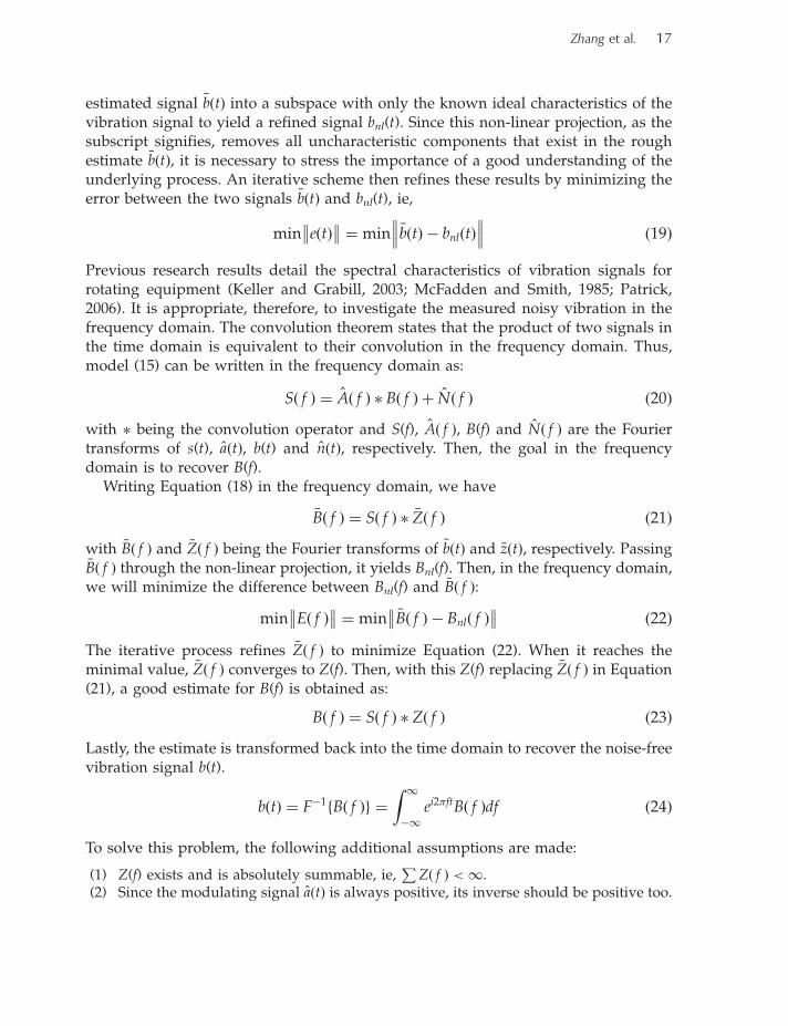
For example, the convergence curve of the cost function versus iteration numberfrom a specific example is illustrated in Figure 15. It can be seen that the cost functionbecomes stable from about the 200th iteration on. Hence, for online applications, theoptimization routine can be terminated after a small number of iterations resulting inconsiderable computational savings.
5.3.4 Simplification of the frequency domain signal convolution: Earlier researchresults (Patrick, 2006) suggest that the main vibration characteristic signature resides infrequency range below 1500 f s Hz, which covers up to six harmonics. In addition, rapidfade of the signal spectra between the harmonics enable us to define Dsup as a series ofwindows on each side of the harmonics. Therefore, Dsup is a collection of six windows
20 Novel blind deconvolution de-noising scheme
with each window being centred at the harmonic frequency and having a certain orderof sidebands on both sides. Then, the convolution operation only considers frequencyspectra on Dsup. To achieve this goal, the convolution operation is divided into threesteps and this process can reduce the computational burden significantly.
Step 1: Picking up frequency spectra on Dsup and separating them into six segmentsas shown in Figure 16. The original signal spectra are shown in Figure 16(a). Theseparated spectra at different harmonics are shown in Figures 16(b)–(g).
Step 2: Convolving each segment with the inverse filter and truncating theconvolution results to the length of each segment as illustrated in Figure 17.Figures 17(a) and (b) show the inverse filer and segment of the measured vibrationsignal (the sidebands at the first harmonic as shown in Figure 16(b), respectively.Figures 17(c) and (d) show the convolution results, before and after the truncation,respectively.
Step 3: Putting the truncated convolution results back to the frequency spectra onDsup to obtain the convolution result.
5.4 Experiments and performance metrics
The signals are normalized and limited within [�1, 1] so that all of them in theproposed scheme can be treated similarly. Since the inverse filter �Zð f Þ is alow-frequency signal and we do not assume any prior knowledge, it is truncated tocontain only 15 spectral lines and assumed to be a simple discrete impulse located atfrequency f s, as shown in Figure 18(a). The optimal inverse filter Z(f) resulting fromthe blind deconvolution scheme is shown in Figure 18(b) for comparison purposes.The large frequency components at 5, 10 and 15 are consistent with the modulatingsignal a(t) for a five-planet-gear plate, whose inverse should show frequencycomponents at 5, 10 and 15, as predicted from the theoretical analysis.
0 100 200 300 400 500 600 700 800 900 10000.4
0.5
0.6
0.7
0.8
0.9
1
Iterations
Cos
t fun
ctio
n va
lue
Figure 15 Convergence of cost function along iterations
Zhang et al. 21

The non-linear projection is given in Equation (12) and is updated in the closed-loop de-noising scheme, shown in Figure 2, with the varying load profile and cracksize. As an example, �Bð f Þ, Bnl(f) and their difference E(f) are shown in Figure 19. E(f) isthe first term in the cost function (25) that must be minimized through theoptimization routine. Finally, in the time domain, the measured noisy vibrationsignal s(t), the noise-free vibration signal recovered from blind deconvolution b(t) andthe noise signal n(t) are shown in Figure 20.
5.4.1 Signal-to-noise ratio: The signal-to-noise ratio (SNR), before and afterde-noising, is investigated and the results at 40% and 100% torque levels are
0 200 400 600 800 1000 1200 14000
0.5
1
1.5
2
2.5
3
3.5
Frequency (order of fs)
Am
plitu
de
210
215
220
225
230
235
240
245
250
0
0.02
0.04
0.06
0.08
0.1
0.12
0.14
0.16
0.18
0.2
Frequency
Am
plitu
de
440 450 460 4700
0.1
0.2
0.3
0.4
0.5
2nd Harmonic
Am
plitu
de670 680 690 700
0
0.5
1
1.5
2
2.5
3
3.5
3rd Harmonic
Am
plitu
de
890 900 910 920 9300
0.2
0.4
0.6
0.8
1
1.2
1.4
1.6
1.8
2
4th Harmonic
Am
plitu
de
1120 1130 1140 1150 11600
0.1
0.2
0.3
0.4
0.5
0.6
0.7
0.8
0.9
1
5th Harmonic
Am
plitu
de
1350 1360 1370 1380 13900
0.05
0.1
0.15
0.2
0.25
0.3
0.35
0.4
6th Harmonic
Am
plitu
de
(a) (b) (c)
(d) (e) (f) (g)
Figure 16 The separation of frequency spectra (with a resolutionof f s): (a) the TSA signal spectra; (b) the first harmonic spectra;(c) the second harmonic spectra; (d) the third harmonic spectra;(e) the fourth harmonic spectra; (f) the fifth harmonic spectra;(g) the sixth harmonic spectra
22 Novel blind deconvolution de-noising scheme

shown in Figures 21(a) and (b), respectively. The improvement in the SNR value is
significant.
5.4.2 Feature performance evaluation: Although the blind deconvolution routineshows a significant improvement in the SNR, it is desirable that it improves also the
quality of the features or condition indicators. The accuracy and precision of
mappings between the evolution of features and the actual crack growth have an
important impact on the performance of diagnostic and prognostic algorithms and the
CBM system overall. To evaluate the quality of the features, several performance
indexes or metrics are introduced.The first performance index is an overall accuracy measure defined as the linear
correlation coefficient between the raw feature values and the crack length growth
along the GAG cycle axis (CCR; Patrick, 2006). Suppose x is the feature vector and
1 5 10 150
0.5
1(a) (b)
Frequency (order of f s)
1 5 10 15
Frequency (order of f s)
Am
plitu
de
0
0.05
0.1
0.15
Am
plitu
de
Figure 18 The spectra of the inverse filter: (a) the initial inversefilter; (b) the optimal inverse filter
0 10 20 300
0.020.040.060.080.1
0.120.140.160.18(a) (b) (c) (d)
Frequency (order of fs)
Am
plitu
de
Am
plitu
de
210 220 230 240 2500
0.10.20.30.40.50.60.70.8
1st Harmonic20
021
022
023
024
025
026
021
021
522
022
523
023
524
024
525
00
0.020.040.060.080.1
0.120.140.160.180.2
Frequency
Am
plitu
de
00.020.040.060.080.1
0.120.140.160.180.2
Frequency
Am
plitu
de
Figure 17 The convolution of the segment of frequency spectra(taking the first harmonic as an example): (a) the inverse filter;(b) the measured vibration signal spectra around the first harmonic;(c) the convolution result; (d) the truncated convolution result
Zhang et al. 23

y the crack growth curve with �x and �y their means, respectively. The correlation
coefficient between them is:
CCRðx, yÞ ¼
ffiffiffiffiffiffiffiffiffiffiffiffiffiffiffiss2
xy
ssxxssyy
sð26Þ
where ssxy ¼Pðxi � �xiÞð yi � �yiÞ, ssxx ¼
Pðxi � �xiÞ
2 and ssyy ¼Pð yi � �yiÞ
2, respec-
tively. The extracted feature will be used to map and predict the crack growth. Hence,
a high correlation coefficient is expected to generate an accurate estimate of the actualcrack length and is preferred. Thus, for a good feature, the value of the correlation
coefficient should be near 1.Because of changes in operating conditions and other disturbances, the feature
values along the GAG axis are often very noisy and need to be smoothed through alow-pass filtering operation. In this case, the correlation coefficient is calculated based
on the smoothed feature curve ~x (CCS; Patrick, 2006). The calculation of CCS is the
0 5000 10,000 15,000 20,000–1
–0.8–0.6–0.4–0.2
00.20.40.60.8
1(a) (b) (c)
Time step
Am
plitu
de
0 5000 10,000 15,000 20,000–1
–0.8–0.6–0.4–0.2
00.20.40.60.8
1
Time step
Am
plitu
de
0 5000 10,000 15,000 20,000–1
–0.8–0.6–0.4–0.2
00.20.40.60.8
1
Time step
Am
plitu
deFigure 20 The estimated vibration signal before and afternon-linear projection and their difference: (a) the measuredvibration signal s(t); (b) the recovered noise-free vibration signalb(t); (c) the noise signal n(t)
0 200 400 600 800 1000 1200 14000
0.050.1
0.150.2
0.250.3
0.350.4
0.450.5(a) (b) (c)
Frequency (order of fs) Frequency (order of fs) Frequency (order of fs)
Am
plitu
de
0 200 400 600 800 1000 1200 14000
0.05
0.1
0.15
0.2
0.25
0.3
0.35
0.4
Am
plitu
de
0 200 400 600 800 1000 1200 14000
0.05
0.1
0.15
0.2
0.25
0.3
0.35
0.4
Am
plitu
de
Figure 19 The results of non-linear projection: (a) �Bð f Þ; (b) Bnl(f);(c) E(f)
24 Novel blind deconvolution de-noising scheme

same as (26) with x being replaced by ~x. In the following experiments, the smoothlow-pass filter is a Butterworth filter with cut-off frequency of 0.01 of the samplingfrequency.
The third performance index is a precision measure corresponding to a normalizedmeasure of the signal dispersion. It is referred to as percent mean deviation (PMD;Patrick, 2006) and defined by:
PMDðx, ~xÞ ¼
Plxi¼1
xi�~xi~xi
lx� 100 ð27Þ
where lx is the number of entities in the feature vector x.In the fault detection and prognostic algorithms (Orchard, 2006), the extracted
feature values are used as a measurement input. Therefore, this performance index isclosely related to the detection threshold and precision of the prognosis results(remaining useful life). From a precise feature, the fault detection and prognosticalgorithms can detect the incipient failure and/or predict the fault growth with a highconfidence. PMD for a precise feature should have a very small value close to 0.
The previous indexes evaluate the performance on the entire failure progressionprocess. It is also important to evaluate how the failure progresses in a small period.To achieve this goal, a moving window along the time axis is applied to the featurevector so that the correlation coefficient and PMD in the moving windows can beevaluated to provide a ‘local’ performance assessment. The two adjacent windows areoverlapped so that the performance indexes in this case are curves along the time axis.
The relative size of the NonRMC sidebands to the RMC sidebands in Dsup or part ofDsup may indicate the presence of a fault on the planetary carrier. As the crack grows,the operating conditions deviates from the ideal. In this case, the constructivesuperposition of vibration signals from different planetary gears is attenuated while
0 100 200 300 400 500 600 700 800 900 1000–4.5
–4
–3.5
–3
–2.5
–2
–1.5
–1
–0.5
GAG
0 100 200 300 400 500 600 700 800 9001000
GAG
Sig
nal-t
o-N
oise
rat
io
SNR of de-noised data
SNR of TSA data
–6.5
–6
–5.5
–5
–4.5
–4
–3.5
–3
–2.5
–2
–1.5
Sig
nal-t
o-N
oise
rat
io
SNR of de-noised data
SNR of TSA data
(a) (b)
Figure 21 The signal-to-noise ratio: (a) Signal-to-noise ratio at40% torque; (b) Signal-to-noise ratio at 100% torque
Zhang et al. 25

the destructive superposition is reinforced. This phenomenon results in smaller RMCand larger NonRMC sidebands. This indicates that the ratio between RMC andNonRMC sidebands can be used as a characteristic feature. Based on this notion,features are successfully extracted in the frequency domain. One of these features, thesideband ratio (SBR; Wu et al., 2004), will be used to demonstrate the effectiveness ofthe de-noising routine.
Let X denote the number of the sidebands in consideration on both sides of thedominant components of the harmonics, the sideband ratio is then defined as the ratiobetween the energy of the NonRMC and all sidebands:
SBRðXÞ ¼
Pmh¼1
PXg¼�X NonRMCPm
h¼1
PXg¼�X ðNonRMCþ RMCÞ
ð28Þ
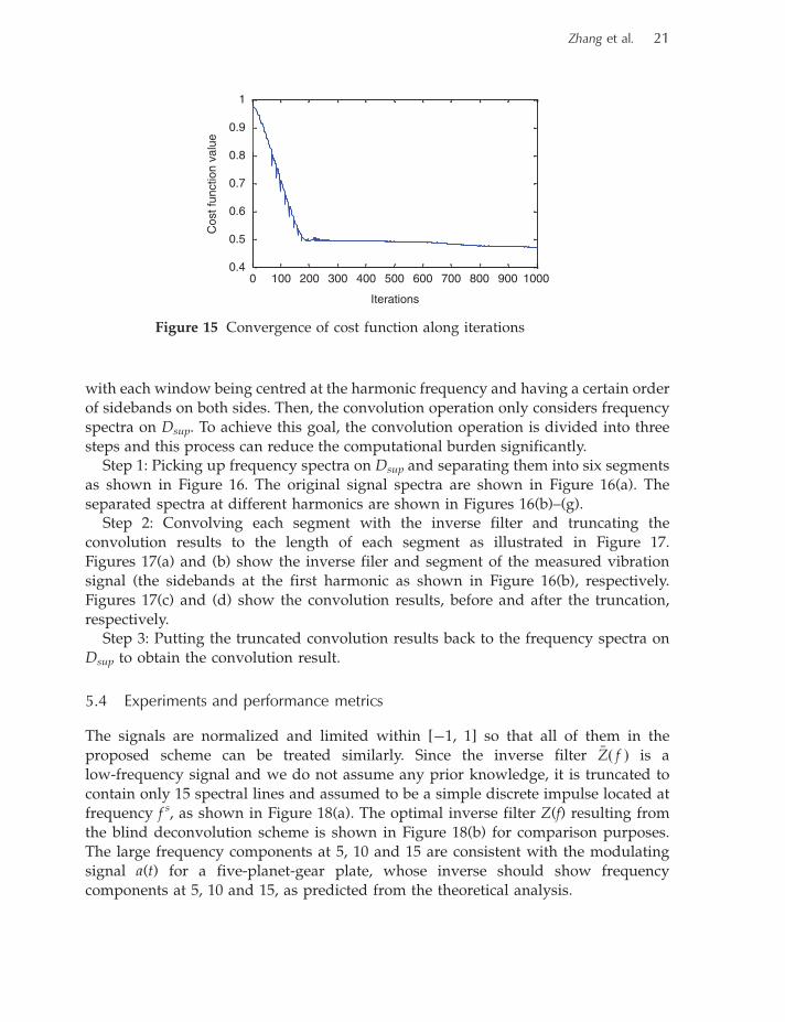
The results of SBR(12) at 40% torque level are shown in Figure 22(a). The runningversion of the performance indexes is shown in Figure 22(b). The results at 100%torque are shown in Figures 22(c) and 22(d), respectively.
The correlation coefficient and PMD for this feature at different torque levels aresummarized in Table 2. Substantial feature improvements are achieved via theapplication of the de-noising routine. In the tables, D-N stands for de-noised.
5.4.3 Failure prognosis: A fault detection/failure prognosis framework based onparticle filtering algorithms has been successfully developed, and applied to theprediction of the remaining useful life (RUL) of the critical components (Orchard,2006). The approach provides with a particle-filter-based estimate of the stateprobability density function (pdf), generates p-step ahead long-term predictions anduses available empirical information about hazard thresholds to estimate the RUL pdf.The implementation of this algorithm requires a failure progression model, featuremeasurements to reveal the failure progression, a non-linear mapping between failureseverity and feature value, and external inputs such as the operational load profile tothe system. More details about this prognosis framework can be found in Orchard(2006). In this section, results are shown to compare the algorithm performance whenusing the features derived in the previous section, before and after de-noising. Thiswill illustrate the efficiency of the proposed de-noising routine, on the prediction ofthe planetary carrier RUL in the helicopter testbed.
Once the RUL pdf is calculated, the performance of failure prognostic algorithm canbe evaluated. For this purpose, statistics such as 95% confidence intervals (CI) andRUL expectations may be used. In our experiment with a seeded crack on theplanetary carrier, failure is defined when the crack reaches 6.21 inches in length, ie, thecrack reaches the edge of the carrier plate. The ground truth data in Table 1 show thatthe crack size reaches this value at the 714th GAG cycle.
Since the gearbox operates on the basis of GAG cycles, the RUL expectations and95% CI are also given with the unit of ‘GAG cycle’. Long-term predictions are
26 Novel blind deconvolution de-noising scheme
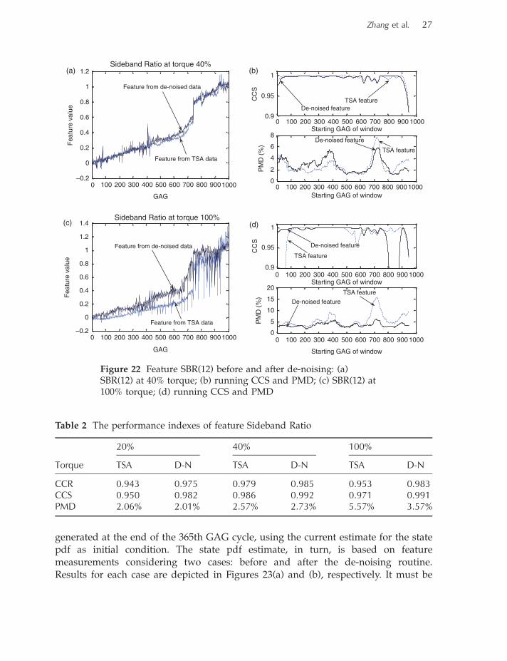
generated at the end of the 365th GAG cycle, using the current estimate for the statepdf as initial condition. The state pdf estimate, in turn, is based on feature
measurements considering two cases: before and after the de-noising routine.
Results for each case are depicted in Figures 23(a) and (b), respectively. It must be
Table 2 The performance indexes of feature Sideband Ratio
20% 40% 100%
Torque TSA D-N TSA D-N TSA D-N
CCR 0.943 0.975 0.979 0.985 0.953 0.983CCS 0.950 0.982 0.986 0.992 0.971 0.991PMD 2.06% 2.01% 2.57% 2.73% 5.57% 3.57%
0 100 200 300 400 500 600 700 800 9001000–0.2
0
0.2
0.4
0.6
0.8
1
1.2(a) (b)
(d)(c)
Sideband Ratio at torque 40%
GAG
Fea
ture
val
ue
Feature from de-noised data
Feature from TSA data
0 100 200 300 400 500 600 700 800 900 10000.9
0.95
1
TSA featurede-noised feature
Starting GAG of window
CC
S
0 100 200 300 400 500 600 700 800 90010000
2
4
6
8
TSA feature
De-noised feature
Starting GAG of window
PM
D (
%)
De-noised featureTSA feature
0 100 200 300 400 500 600 700 800 9001000–0.2
0
0.2
0.4
0.6
0.8
1
1.2
1.4
GAG
Fea
ture
val
ue
Sideband Ratio at torque 100%
Feature from de-noised data
Feature from TSA data
0 100 200 300 400 500 600 700 800 900 10000.9
0.95
1
TSA feature
De-noised feature
Starting GAG of window
CC
S
0 100 200 300 400 500 600 700 800 900 10000
5
10
15
20TSA feature
De-noised feature
Starting GAG of window
PM
D (
%)
Figure 22 Feature SBR(12) before and after de-noising: (a)SBR(12) at 40% torque; (b) running CCS and PMD; (c) SBR(12) at100% torque; (d) running CCS and PMD
Zhang et al. 27

noted that the 95% CI in both scenarios are quite similar precision-wise. However, theRUL expectation is closer to the ground truth value when a de-noised feature is used,
showing that the de-noise routine improves the accuracy of the algorithm.As time goes on, differences between the two cases become evident. Table 3
summarizes the results obtained when performing the prognostic algorithm at the400th, 450th and 500th GAG cycles, respectively. In terms of precision of the prediction,
it is clear that prognosis results with the de-noised feature offer a considerable
reduction in the length of the 95% CI. For instance, when the long-term prediction is
0 100 200 300 400 500 600 700 8000
2
4
6
8Particle filters: Non-linear system state prediction
Cra
ck le
ngth
gro
wth
0 100 200 300 400 500 600 700 8000
0.2
0.4
0.6
0.8
1
Normalized probability density function of TTF [GAG cycles]
Number of GAG cycles
0 100 200 300 400 500 600 700 8000
2
4
6
8Particle filters: Non-linear system state prediction
Cra
ck le
ngth
gro
wth
0 100 200 300 400 500 600 700 8000
0.2
0.4
0.6
0.8
1
Normalized probability density function of TTF [GAG cycles]
Number of GAG cycles
(a) (b)
Figure 23 Prognosis results started from the 365th GAG cycle:(a) prognosis based on TSA feature; (b) prognosis based onde-noised feature
Table 3 The performance indexes of failure prognosis
Initial GAG cycle for long-term prediction
Feature Performance 365 400 450 500
TSA 95% CI [637–773] [663–832] [680–828] [682–812]Length of CI 136 169 148 130Expected value 705 747 754 747
De-noised 95% CI [638–777] [647–775] [618–720] [695–784]Length of CI 139 128 102 89Expected value 710 711 670 746
28 Novel blind deconvolution de-noising scheme

performed at the 450th GAG cycle, this reduction is in the order of about 140 min(46 GAG cycles). At the same time, the expected values for the RUL obtained from thede-noised feature are also more accurate that those from the TSA feature. It is importantto note that, in real applications, a predicted failure time lower than the actual one ispreferred since it does not involve the risk of continuing the operation beyond safety.A lower failure time prediction only makes a conservative decision to schedulemaintenance earlier, but a higher value of the failure time in the prediction mightpostpone the timely maintenance, resulting in damage or loss of vehicle.
6. Conclusions
The successful implementation of CBM technologies is achieved through theapplication of a failure prognostic algorithm, which in turn requires a high-qualityfeature to propagate the failure in time with respect to the operating conditions of thesystem. Good features are often extracted from vibration signals collected from a noisyenvironment and noise might mask the signatures of the faults/failures. Therefore,signal de-noising and preprocessing is important in the implementation of CBM.This paper introduce the development of a new vibration signal blind deconvolutionde-noising scheme in synergy with feature extraction, failure prognosis and vibrationmodelling to improve the signal-to-noise ratio, the quality of features, as well as theaccuracy and precision of failure prognostic algorithms. The proposed scheme isapplied to the failure prognosis of a critical component of a helicopter testbed and theresults demonstrate the efficiency of the proposed scheme.
Acknowledgements
The research reported in this paper was partially supported by DARPA and NorthropGrumman under the DARPA Prognosis program Contract No. HR0011-04-C-003. Wegratefully acknowledge the support and assistance received from our sponsors.
This paper should have been included in the themed issue on diagnostics and prognosticsthat was published in the June–August double issue 2009, volume 31 issue 3–4.
ReferencesAntoni, J. 2005: Blind separation of vibration
components: principles and demonstrations.Mechanical Systems and Signal Processing 19,1166–80.
Antoni, J. and Randall, R. 2004: Unsupervisednoise cancellation for vibration signals: part I –evaluation of adaptive algorithms. MechanicalSystems and Signal Processing 18, 89–101.
Ayers, G.R. and Dainty, J.C. 1988: Iterativeblind deconvolution method and its applica-tions. Optics Letters 13, 547–49.
Gelle, G., Colas, M. and Delaunay, G. 2000:Blind sources separation applied to rotatingmachines monitoring by acoustical andvibrations analysis. Mechanical Systems andSignal Processing 14, 427–42.
Hillerstrom, G. 1996: Adaptive suppression ofvibrations – a repetitive control approach, IEEETrans. Control Systems Technology 4(1): 72–78.
Keller, J. and Grabill, P. 2003: Vibrationmonitoring of a UH-60A main transmissionplanetary carrier fault. The American Helicopter
Zhang et al. 29

Society 59th Annual Forum, Phoenix, AZ, May,1–11.
Klamecki, B. 2005: Use of stochastic resonancefor enhancement of low-level vibrationsignal components. Mechanical Systems andSignal Processing 19, 223–37.
Kundur, D. and Hatzinakos, D. 1998: A novelblind deconvolution scheme for image resto-ration using recursive filtering. IEEETransactions on Signal Processing 26, 375–90.
Lebold, M., McClintic, K., Campbell, R.,Byington, C. and Maynard, K. 2000:Review of vibration analysis methods forgearbox diagnostics and prognostics.Proceedings of the 54th Meeting of the Societyfor Machineary Failure Prevention Technology,Virginia Beach, VA, May, 623–34.
McFadden, P. and Smith, J. 1985: An explana-tion for the asymmetry of the modulationsidebands about the tooth meshing frequencyin epicyclic gear vibration. Proceedings of theInstitution of Mechanical Engineers, Part C:Mechanical Engineering Science 199, 65–70.
Nandi, A.K., Mampel, D. and Roscher, B.1997: Blind deconvolution of ultrasonic sig-nals in nondestructive testing applications.IEEE Transactions on Signal Processing 45,1382–90.
Orchard, M. 2006: A particle filtering-basedframework for online fault diagnosis andfailure prognosis. PhD proposal, School ofElectrical and Computer Engineering,Georgia Institute of Technology, Atlanta, GA.
Patrick, R. 2006: A model-based framework forfault diagnosis and prognosis of dynamical
system with an application to helicopter trans-missions. PhD proposal, School of Electricaland Computer Engineering, Georgia Instituteof Technology, Atlanta, GA, September.
Peled, M.Z.R. and Braun, S. 2005: A blinddeconvolution separation of multiplesources, with application to bearing diag-nostics. Mechanical Systems and SignalProcessing 19, 1181–95.
Prost, R. and Goutte, R. 1984: Discrete con-strained iterative deconvolution with opti-mized rate of convergence. Signal Processing7, 209–30.
Saxena, A., Wu, B. and Vachtsevanos, G. 2005:A methodology for analyzing vibration datafrom planetary gear system using complexMorelt wavelets. Proceedings of the AmericanControl Conference, vol. 7, Portland, OR, June,4730–35.
Szczepanik, A. 1989: Time synchronous aver-aging of ball mill vibrations. MechanicalSystems and Signal Processing 3, 99–107.
Vachtsevanos, G., Lewis, F., Roemer, M.,Hess, A. and Wu, B. 2006: Intelligent faultdiagnosis and prognosis for engineering systems.Wiley.
Wu, B., Saxena, A., Khawaja, T., Patrick, R.,Vachtsevanos, G. and Sparis, R. 2004: Anapproach to fault diagnosis of helicopterplanetary gears. IEEE AUTOTESTCON, SanAntonio, TX, September, 475–81.
Wu, B., Saxena, R.P.A. and Vachtsevanos, G.2005: Vibration monitoring for fault diagno-sis of helicopter planetary gears. IFAC WorldCongress, Prague, July.
30 Novel blind deconvolution de-noising scheme
Recommended