Research Article Open Access
Bondarenko and Bondarenko, Int J Swarm Intel Evol Comput 2017, 6:1DOI: 10.4172/2090-4908.1000149
Research Article OMICS International
International Journal of Swarm Intelligence and Evolutionary ComputationInternatio
nal J
ourn
al o
f Swarm
Intelligence and Evolutionary Computation
ISSN: 2090-4908
Volume 6 • Issue 1 • 1000149Int J Swarm Intel Evol Comput, an open access journalISSN: 2090-4908
Keywords: Stochastic model; Fractional Brownian motion; Estimation of parameters
IntroductionLet [ ]( ), 0,x t t T∈ is an observed trajectory, which is describing
the stochastic evolution of some dynamic object. Mathematical model of this trajectory is defined as a random process, )(tξ . Where:
⋅x(t) = X(t), X( ) is realization of the processξ .
As a rule, we chose as a model random process with known characteristics. Direct use of this definition requires broad classes of these processes. On the other hand, this class includes Gauss and Markov processes. Let's introduce another definition of continuous mathematical models for the observed trajectory );0()( TCx ∈⋅ using nonlinear conversion.
DefinitionMathematical model of observed trajectory x (t) is a pair ),( ξΦ , where
x(t) (X( ))(t),= Φ ⋅ )(tξ is a random process with known characteristics, Φ is a reversible conversion in (0, t)c .
Let’s assume ,,..,1, nktt k == ,0,0)1( 11 =−
−+= tn
Tkttk )))((( kk tXx ⋅Φ= is a model of observed time series ....1 nxx
Let’s call ξ as a basic process of the model. Levy processes with independent stationary increments have been considered as basic for models of time series (particularly financial) [1-4]. The next step in the development of the models is transition to diffusion processes. For example, diffusion model of stock price )(tS is obtained from the following considerations:
})(exp{)0()( ttwStS µσ += , X(t)=1n S(t),
Where (t)w is a standard Wiener process, σ is volatility and interest rate, µ is a constant. Then let’s propose the equation:
( ) S(t) ( ) ( )dS t dw t S t dtσ µ= +
Which can be interpreted as a stochastic equation Ito and its solution could be written as a geometric (economic) Brownian motion:
−+= ttwStS
2)(exp)0()(
2σµσ (1)
For the model (1) of a stock price have been obtained a number of known results, including the Black-Scholes formula for a rational option pricing [5-8]. The main drawback of Levy processes (and diffusion) is their Markov. Thus, the Markov property:
===∆∈ −− })(,..,)()({ 1111 nnn atXatXtXP
))()(( 11 −− =∆∈= nnn atXtXP
A priori satisfies only the simplest physical phenomena. The absence of impact on processes in biology, economics, climate, etc. looks unconvincing. In this paper we propose a non-Markovian model of the time series.
Selection of the Base Process and its PropertiesOne of the most popular Markov models of time series is Gaussian
random process, and fractional Brownian motion [9-11]. The demand of this process is caused by "convenient" properties, which are described below.
Fractional Brownian motion is defined as a Gaussian random process with characteristics:
BH (t), )(21)()(,0)0(,0)( 222 HHH
HHHH ststsBtBBtB −−+=Ε==Ε )(21)()(,0)0(,0)( 222 HHH
HHHH ststsBtBBtB −−+=Ε==Ε
Note that with 5,0=H we get a standard Wiener process.
Smoothness of the trajectories of the process )(tBH is defined by the parameter H: almost all the trajectories satisfy the Holder condition:
α−≤− stcsXtX )()( , ,H<α
This generalizes known Levy’s result for the Wiener process.
The increments of fbm )()( 12 tBtB HH − , )()( 34 tBtB HH − ,1 2 3 4t t t t< < < are form a Gaussian random vector with a correlation
between the coordinates:
))()()()((21 2
132
242
232
14HHHH tttttttt −−−−−+−
For discrete time:
)1()(n
kBnkB HHk
−−=ξ ,
We obtain the correlation coefficient:
*Corresponding author: Valeria Bondarenko, Department of IRCYYN, Ecole Centrale de Nantes, France, Tel: +330785414501; E-mail: [email protected]
Received January 14, 2017; Accepted February 21, 2017; Published February 28, 2017
Citation: Bondarenko V, Bondarenko V (2017) The Model of Real Data Constructing Using Fractional Brownian Motion. Int J Swarm Intel Evol Comput 6: 149. doi: 10.4172/2090-4908.1000149
Copyright: © 2017 Bondarenko V, et al. This is an open-access article distributed under the terms of the Creative Commons Attribution License, which permits unrestricted use, distribution, and reproduction in any medium, provided the original author and source are credited.
AbstractIn this paper we investigate the properties of the fractional Brownian motion as a basic process of stochastic
time series models. New method of estimating the Hurst exponent is substantiated. Stochastic model, which is representing a time series analysis in the form of increments converted to fractional Brownian motion. The method of checking the adequacy of the proposed models. The research results are implemented in software for the simulation and analysis temporal data.
The Model of Real Data Constructing Using Fractional Brownian MotionValeria Bondarenko1* and Victor Bondarenko2
1Department of IRCYYN, Ecole Centrale de Nantes, France2Department of Applied System Analysis, National Technical University of Ukraine KPI, Ukraine
Citation: Bondarenko V, Bondarenko V (2017) The Model of Real Data Constructing Using Fractional Brownian Motion. Int J Swarm Intel Evol Comput 6: 149. doi: 10.4172/2090-4908.1000149
Page 2 of 7
Volume 6 • Issue 1 • 1000149Int J Swarm Intel Evol Comput, an open access journalISSN: 2090-4908
),211(21),( 222 HHH
kj jkjkjk −−−−++−=ξξρ ), (2)
It means that increments are forming stationary (in the narrow sense) sequence [12].
Let's mention some several properties of fBm:
1. Changing time scale is equivalent for changing of "amplitude” of the process:
Law(BH(at))= Law(aHBH(t)),
This equality denotes the coincidence of one-dimensional distributions of the processes:
BH(ta) and )(tBa HH
This property is called self-similarity process and it is useful for analysis of time series.
2. Let's put in the formula (2): j=k+n. Then the correlation coefficient:
).2)1()1((21),( 222 HHH
nkk nnn −−++=+ξξρ ), (3)
),( nkkn += ξξρρ ~ ,)12( 22 −− HnHH (4)
So the memory decreasing for increments has a power character; the increments are independence with
21
=H . With 21
<H the increments are form the sequence with short,
21
>H with a long memory. The sign of correlation coefficient nρ , which is defined by formula (4), depends form value H :
21,0 << Hnρ ,
21,0 >> Hnρ . For 2
1<H
sequence nξ of increments fbm is calling pink noise and negativity of variations means the fast variability values. The process of fbm 2
1<H
is known as anti-persistent. For 21
>H sequence ny of increments fbm is calling black noise and process of fbm is known as persistent. The properties of persistence have data which are describing some of the physical processes, such as solar activity [13,14].
In this paper, is selected fractional Brownian motion as a basic process.
The Statistics of Fractional Brownian motionThe estimation of Hurst exponent
Let’s observe the data:
1−= σ = −k H k k kkx B ( ), y x xn
Let’s random vector),0(~),..,,( 21 Vyyy n ℵ=y , where the correlation matrix
Sn
V H2
2σ= and elements Sjk of matrix HSS ≡ is defined by equality (3).
The limit theorems for sequence nyy ,..,1 were first proved by Peltier for statistics [15].
jn
kkjn y
nR ∑
==
1
1
, j ∈ IR
πσ
+Γ
=Ε=Ε 212
)(2 j
nRj
j
jH
j
jnn ,
With probability 1
1)(→
Ε jR
n
jn
, ∞→n (5)
From (5) is follows consistency estimates of parameters :,σH
^1
21n
1nn
n
RH
n
=
σπ
With known :σ
1 1 11 252π
σ = =H Hn n nˆ n rR , n R (6)
With known H.
Let’s propose new method of estimation Hurst exponent [16-18].
Let’s introduce the notation:
nyyS
RHQ
n
),(8,0)(1
1
−=
Where matrix HSS ≡ is defined.
Statement
Statistic
1)(minargˆ −= HQH
Is a consistent estimator of the parameter H.
Proofε
Is the canonical Gaussian vector with the following characteristics:
.dim),(),(),(,0 nvuvu ==Ε=Ε εεεε
Then12y V= ε , therefore
( ) ( ) ( )2
1 12E , E , E ,Hnn V y y s y y− −= = =ε ε
σAnd consequently the statistic
22ˆ nσ = ),()( 112 yy−− Sn H
And here statistics ),()( 112 yySn H −− is an unbiased estimate of the parameter
2σ . Let’s introduce:
),(ˆ 1122 yy−−= Sn H
nσ (7)
With calculating the dispersion421242
2 ),(ˆ σσ −Ε= −− yySnD Hn
Use the formula for integration by parts for the Gaussian measure [19] and get
02ˆ4
22 →=
nD n
σσ , ∞→n
n2σ Is a consistent parameter estimation ofσ .
The equalities (6,7) are form the system, from which follows the relation:
1),(8,0ˆˆ 1
11
2 ≈=−
nS
R nn
n yyσσ
, min1
ˆˆ
1
2 →−n
n
σσ
This proves the statement. The efficiency of proposed estimation method has been tested by numerical experiment [16].
The limit theorems for some statistics
The limit theorems for statistics from increments of fractional Brownian motion have been proved in works of Nourdin I and others [20-23].
Citation: Bondarenko V, Bondarenko V (2017) The Model of Real Data Constructing Using Fractional Brownian Motion. Int J Swarm Intel Evol Comput 6: 149. doi: 10.4172/2090-4908.1000149
Page 3 of 7
Volume 6 • Issue 1 • 1000149Int J Swarm Intel Evol Comput, an open access journalISSN: 2090-4908
1 ~ (0;1)Hk
k kn B Bn n
ξ − = − ℵ
Let’s denote
∑−
==
=
1
1
k
jj
Hk n
kBn ξα
There is a Mean-square convergence:
231 3
1−→∑
=k
n
kknξα
,
∈
21;0H
(8)
ηξα 31 321 →∑+ kkHn
∈
21;0H
(9)
Where
+ℵ
221;0~
Hη
;
)1(231 23
12 B
n k
n
kkH →∑
=ξα
,
∈ 1;
21H
(10)
These results allow us to estimate the adequacy of model with the basic process-fractional Brownian motion.
Construction and Checking the Adequacy of ModelIt requires initial analysis of increments{ }nyy ,..,1 to determine the
conversionΦ .
In particular, is it necessary to estimate the one-dimensional distribution of sample and correlation. These actions are possible only with a large sample size (n>5000). We propose new empirical method of transformation increments { }nyy ,..,1 in { }nzz ,..,1 for small sample.
The first stage of approximation is an empirical method for testing the hypothesis about normality increments of model. The criterion may be Gaussian value "kurtosis" (excess kurtosis):
∑
∑
=
=
−
−
= n
kk
n
kk
n
yn
ynd
2
2
2
2
11
||1
1
,
Which is equal π2
for Gaussian model. If nd is significantly
different from π2 , let's replace the time series 11.. −nyy by the new
sequence 11.. −nzz .
The general idea of approximation is an one-dimensional functional transformation g of each increment ky , where g is an increasing odd function,
)( kk ygz =
Let’s assume
π2
))((1
1
)(1
1
lim 1
1
2
21
1 =
−
−
∑
∑−
=
−
=
∞→ n
kk
n
kk
nyg
n
ygn
,
Where )( kk ygz = is assumed as a Gaussian random value. Let’s demonstrate proposed algorithm with g as a power function. Assume
)(sgn 11
kkkk yyyz −Φ== λ……………………….. (11)
)(sgn kkkk zzyy Φ== λ 0>λ , ………………… (11A)
Then
∑
∑−
=
−
=
−
−= 1
1
2
21
1
11
11
n
kk
n
kk
n
zn
zn
dλ
λ
nndd
∞→= lim Is equal to ratio of the corresponding mathematical
expectations. For );0(~ 2σξ ℵ
+
Γ=Ε2
12 2 ασπ
ξ α
α
α
, then
+Γ
+Γ
=
21
21
12
λ
λ
πd
Where the parameter 𝛌 is defined from the equation. Thus, the proposed approximation leads to the following model of original time series:
λ||sgn
1j
k
jjk zyx ⋅= ∑
=
If we'll assume that values of sequence { }nzz ,..,1 are increments of fBm, let’s calculate Hurst exponent by the following algorithm, which shows proposed method:
1) Construct the statistic:
zz
nR k == ∑1
1
2) Calculate the matrix1−
Hs , where HS is a correlation matrix of increments:
1 1− −= Ε − − = ρ ξ ξjk H H H H j k
k k j js ( B ( ) B ( ))( B ( ) B ( )) ( , )n n n n
1),(8,0 1
1 −=
−
nS
RQ H zz
,
The statistics Q is calculating for difference values of Hurst exponent with step (0, 0.5-1) and:
min,1)( →−HQ 1= −H arg min Q( H ) (12)
3) The testing of hypothesis T= (statistics nzz ,..,1 which obtained by transformation (11) of real data are simulated by increments from fractional Brownian motion). The algorithm with known H is the following. Denote
∑=
=n
kkz
nc
1
21
And assume that hypothesis Т is done
−
+
==nkB
nkBnccz H
kk1ξ
Assume ∑−
==
1
1
k
jjk zv and construct the statistics
31kkn zv
nA ∑=
,
∈
21;0H
;
Citation: Bondarenko V, Bondarenko V (2017) The Model of Real Data Constructing Using Fractional Brownian Motion. Int J Swarm Intel Evol Comput 6: 149. doi: 10.4172/2090-4908.1000149
Page 4 of 7
Volume 6 • Issue 1 • 1000149Int J Swarm Intel Evol Comput, an open access journalISSN: 2090-4908
3211
kkHn zvn
B ∑+=,
∈
21;0H
; (13)
321
kkHn zvn
D ∑=,
∈ 1;
21H
If hypothesis T is true, there is convergence:2
23 cAn −→
; η25
3cBn → ; )1(
23 22BcDn →
The decision about hypothesis T is accepted by comparing the real values of the statistics with their theoretical limit values. Let's determine deviation from the limit values for statistic nA .
AAAn −=δ
The limit distribution functions for statistics nB , nD
{ } )3
(3)( 5,25,21
−Φ=<= cxxcPxFσ
η,
,0,1)321(2)(2 >−Φ= xx
cxF
Where Φ is Laplace function, 5,0)22( −+= Hσ
The hypothesis T is accepted, if:
5,0,0:5,0,, 210 ><<<<< HDHB nn βββδ (14)
Where 21,ββ are quantile distributions from 21, FF which corresponding to the selected significance level .1,0=α
2 52 2
1 24 95 4 082 2
β = β = =+
,, c , , c ,c zH
The Real ExamplesLet’s consider examples of real nature:
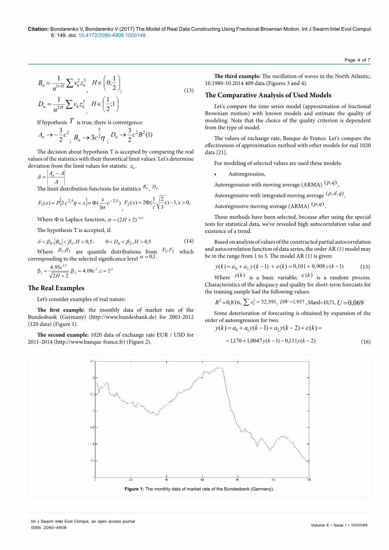
The first example: the monthly data of market rate of the Bundesbank (Germany) (http://www.bundesbank.de) for 2003-2012 (120 data) (Figure 1).
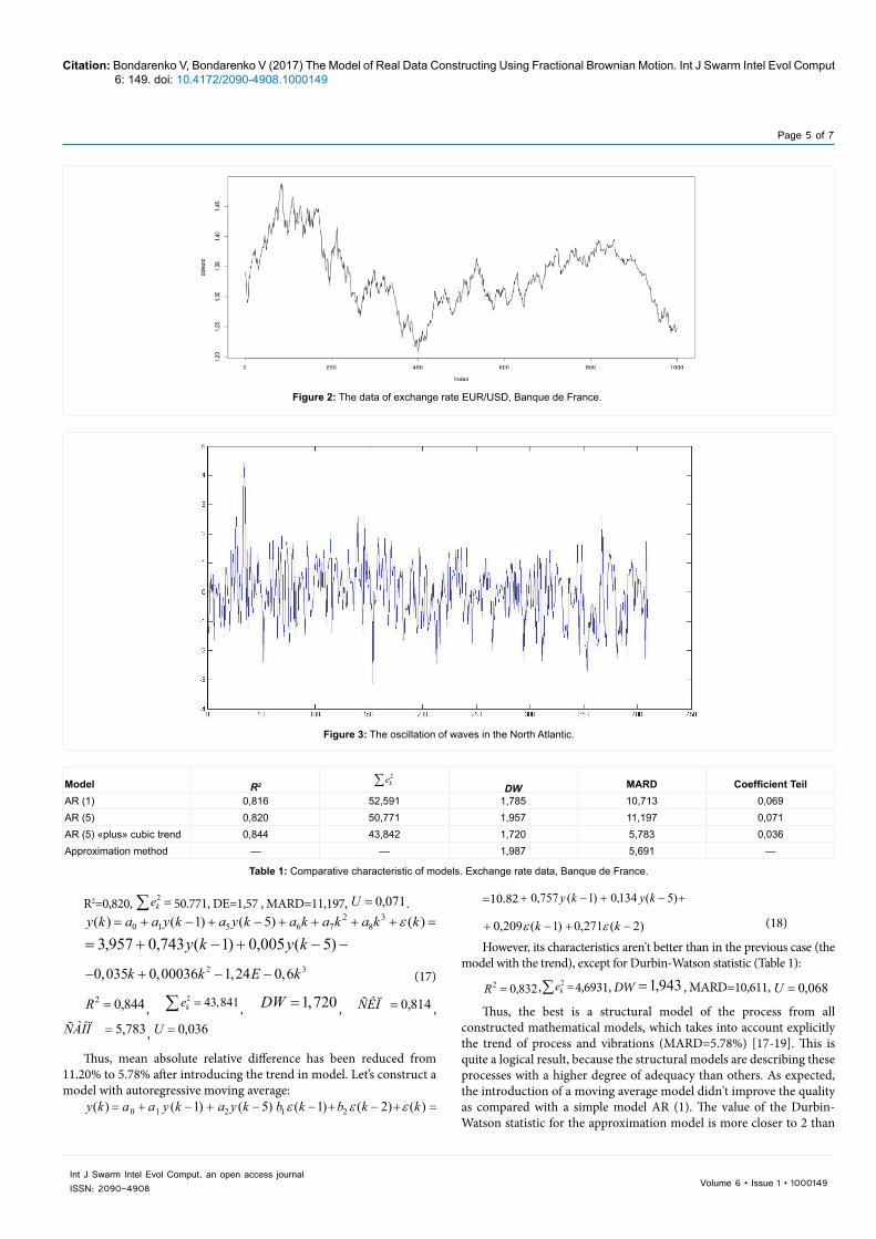
The second example: 1020 data of exchange rate EUR / USD for 2011-2014 (http://www.banque-france.fr) (Figure 2).
The third example: The oscillation of waves in the North Atlantic, 10.1980-10.2014 409 data (Figures 3 and 4).
The Comparative Analysis of Used ModelsLet's compare the time series model (approximation of fractional
Brownian motion) with known models and estimate the quality of modeling. Note that the choice of the quality criterion is dependent from the type of model.
The values of exchange rate, Banque de France. Let's compare the effectiveness of approximation method with other models for real 1020 data [21].
For modeling of selected values are used these models:
• Autoregression,
Autoregression with moving average (ARMA) ),( qp ,
Autoregressive with integrated moving average ),,( qdp ,
Autoregressive moving average (ARMA) ),( qp .
These methods have been selected, because after using the special tests for statistical data, we've revealed high autocorrelation value and existence of a trend.
Based on analysis of values of the constructed partial autocorrelation and autocorrelation function of data series, the order AR (1) model may be in the range from 1 to 5. The model AR (1) is given:
=+−+= )()1()( 10 kkyaaky ε )1(908,0101,0 −+= ky (15)
Where )(ky is a basic variable; )(kε is a random process. Сharacteristics of the adequacy and quality for short-term forecasts for the training sample had the following values:
816,02 =R , 2 52 591=∑ ke , , 1 957=DW , , Mard=10,71, 069,0=USome deterioration of forecasting is obtained by expansion of the
order of autoregression for two:=+−+−+= )()2()1()( 210 kkyakyaaky ε
)2(111,0)1(0047,1176,1 −−−+= kyky (16)
Figure 1: The monthly data of market rate of the Bundesbank (Germany).
Citation: Bondarenko V, Bondarenko V (2017) The Model of Real Data Constructing Using Fractional Brownian Motion. Int J Swarm Intel Evol Comput 6: 149. doi: 10.4172/2090-4908.1000149
Page 5 of 7
Volume 6 • Issue 1 • 1000149Int J Swarm Intel Evol Comput, an open access journalISSN: 2090-4908
R2=0,820, 771,502 =∑ ke 50.771, DE=1,57 , MARD=11,197, 071,0=U .=++++−+−+= )()5()1()( 3
82
76510 kkakakakyakyaaky ε
−−+−+= )5(005,0)1(743,0957,3 kyky2 30,035 0,00036 1,24 0,6k k E k− + − − (17)
844,02 =R , 2 43,841=∑ ke , 1,720=DW , 814,0=ÑÊÏ ,
783,5=ÑÀÎÏ , 036,0=U
Thus, mean absolute relative difference has been reduced from 11.20% to 5.78% after introducing the trend in model. Let’s construct a model with autoregressive moving average:
=+−+−−+−+= )()2()1()5()1()( 21210 kkbkbkyakyaaky εεε
Figure 2: The data of exchange rate EUR/USD, Banque de France.
Figure 3: The oscillation of waves in the North Atlantic.
=10.82 +−+−+= )5(134,0)1(757,082,10 kyky
)2(271,0)1(209,0 −+−+ kk εε (18)
However, its characteristics aren't better than in the previous case (the model with the trend), except for Durbin-Watson statistic (Table 1):
832,02 =R , 931,462 =∑ ke 4,6931, DW 943,1=DW , MARD=10,611, 068,0=U
Thus, the best is a structural model of the process from all constructed mathematical models, which takes into account explicitly the trend of process and vibrations (MARD=5.78%) [17-19]. This is quite a logical result, because the structural models are describing these processes with a higher degree of adequacy than others. As expected, the introduction of a moving average model didn't improve the quality as compared with a simple model AR (1). The value of the Durbin-Watson statistic for the approximation model is more closer to 2 than
Model R2 ∑ 2ke
DW MARD Coefficient TeilАR (1) 0,816 52,591 1,785 10,713 0,069AR (5) 0,820 50,771 1,957 11,197 0,071АR (5) «plus» cubic trend 0,844 43,842 1,720 5,783 0,036Approximation method — — 1,987 5,691 —
Table 1: Comparative characteristic of models. Exchange rate data, Banque de France.
Citation: Bondarenko V, Bondarenko V (2017) The Model of Real Data Constructing Using Fractional Brownian Motion. Int J Swarm Intel Evol Comput 6: 149. doi: 10.4172/2090-4908.1000149
Page 6 of 7
Volume 6 • Issue 1 • 1000149Int J Swarm Intel Evol Comput, an open access journalISSN: 2090-4908
the other models, the value of MARD is practically coincides with its value for the AR (5) "plus" cubic trend.
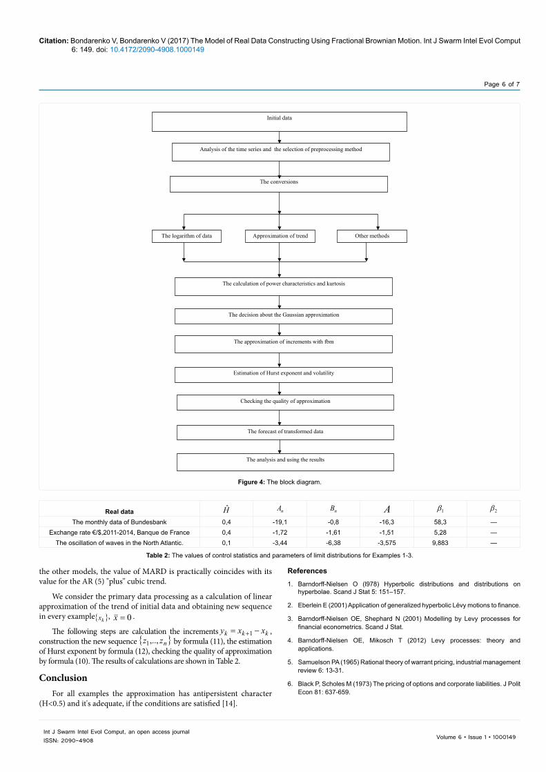
We consider the primary data processing as a calculation of linear approximation of the trend of initial data and obtaining new sequence in every example{ }kx , 0=x .
The following steps are calculation the increments kkk xxy −= +1 , construction the new sequence { }nzz ,..,1 by formula (11), the estimation of Hurst exponent by formula (12), checking the quality of approximation by formula (10). The results of calculations are shown in Table 2.
ConclusionFor all examples the approximation has antipersistent character
(H<0.5) and it's adequate, if the conditions are satisfied [14].
Initial data
Analysis of the time series and the selection of preprocessing method
The conversions
The logarithm of data Approximation of trend Other methods
The calculation of power characteristics and kurtosis
The decision about the Gaussian approximation
The approximation of increments with fbm
Estimation of Hurst exponent and volatility
Checking the quality of approximation
The forecast of transformed data
The analysis and using the results
Figure 4: The block diagram.
Real data H nA nB A 1β 2β
The monthly data of Bundesbank 0,4 -19,1 -0,8 -16,3 58,3 —Exchange rate €/$,2011-2014, Banque de France 0,4 -1,72 -1,61 -1,51 5,28 —
The oscillation of waves in the North Atlantic. 0,1 -3,44 -6,38 -3,575 9,883 —
Table 2: The values of control statistics and parameters of limit distributions for Examples 1-3.
References
1. Barndorff-Nielsen O (l978) Hyperbolic distributions and distributions on hyperbolae. Scand J Stat 5: 151–157.
2. Eberlein E (2001) Application of generalized hyperbolic Lévy motions to finance.
3. Barndorff-Nielsen OE, Shephard N (2001) Modelling by Levy processes for financial econometrics. Scand J Stat.
4. Barndorff-Nielsen OE, Mikosch T (2012) Levy processes: theory and applications.
5. Samuelson PA (1965) Rational theory of warrant pricing, industrial management review 6: 13-31.
6. Black P, Scholes M (1973) The pricing of options and corporate liabilities. J Polit Econ 81: 637-659.

Citation: Bondarenko V, Bondarenko V (2017) The Model of Real Data Constructing Using Fractional Brownian Motion. Int J Swarm Intel Evol Comput 6: 149. doi: 10.4172/2090-4908.1000149
Page 7 of 7
Volume 6 • Issue 1 • 1000149Int J Swarm Intel Evol Comput, an open access journalISSN: 2090-4908
7. Merton RC (1973) Theory of rational option pricing. Bell J Econ 4: 141-183.
8. Black F (1988) The holes in Black-Scholes. Risk Magazine 1:30-33.
9. Mandelbrot BB (1965) Une classe de processus stochastiques homothetiques asoi: Application a la loi climatologique de H. E. Hurst, Comptes Rendus de l'Academie des Sciences, Paris 240: 3274-3277.
10. Mandelbrot BB, Van-Ness JW (1968) Fractional Brownian motions, fractional noises and applications, Slam Review. 10: 422-437.
11. Gusak D, Kukush A, Kulik A, Mishura Yu, Pilipenko A (2010) Theory of stochastic processes with applications to financial mathematics and risk theory. Springer, p: 380.
12. Mandelbrot B (1982) The Fractal Geometry of Nature, Freeman and Co., San Francisco 89: 460.
13. Beran J (1995) Statistics for Long-Memory Processes. Chapman and Hall, p: 315.
14. Mishura Y (2008) Stochastic calculus for fractional Brownian motion and related processes. Lecture notes in Mathematics.
15. Peltier RF (1994) A new method for estimating the parameter of fractional Brownian motion. Rapport de recherché de l’INRIA. 27.
16. Coeurjolly JF (2000) Simulation and identification of the fractional Brownian motion: A bibliographical and comparative study. J Stat softw 5: 1-52.
17. Coeurjolly JF (2001) Estimating the parameters of a fractional Brownian motion by discrete variations of its sample paths. Stat Inference Stoch Process 4: 199-227.
18. Coeurjolly JF (2008) Hurst exponent estimation of locally self-similar Gaussian processes using sample quantiles. Ann. Stat. 36: 1404-1434.
19. Korolyuk V, Limnios N, Mishura Y, Sakhno L, Shevchenko G (2014) Modern stochastics and applications.
20. Nourdin I (2008) Asymptotic behaviour of weighted quadratic and cubic variations of fractional Brownian motion. Ann. Probab. 36: 2159-2175.
21. Nourdin I (2009) Non-central convergence of multiple integrals. Ann. Probab. 37: 1412-1426.
22. Nourdin I (2009) Density formula and concentration inequalities with Malliavin calculus. Electron J Probab 14: 2287-2300.
23. Nourdin I (2010) Central and non-central limit theorems for weighted power variations of fractional Brownian motion. Ann. Inst H. Poincaré Probab Statist 46: 1055-1079.
Citation: Bondarenko V, Bondarenko V (2017) The Model of Real Data Constructing Using Fractional Brownian Motion. Int J Swarm Intel Evol Comput 6: 149. doi: 10.4172/2090-4908.1000149
OMICS International: Open Access Publication Benefits & FeaturesUnique features:
• Increased global visibility of articles through worldwide distribution and indexing• Showcasing recent research output in a timely and updated manner• Special issues on the current trends of scientific research
Special features:
• 700+ Open Access Journals• 50,000+ editorial team• Rapid review process• Quality and quick editorial, review and publication processing• Indexing at major indexing services• Sharing Option: Social Networking Enabled• Authors, Reviewers and Editors rewarded with online Scientific Credits• Better discount for your subsequent articles
Submit your manuscript at: http://www.omicsonline.org/submission
Recommended