A STOCHASTIC PARAMETER REGRESSION MODEL
FOR LONG MEMORY TIME SERIES
by
Rose Marie Ocker
A thesis
submitted in partial fulfillment
of the requirements for the degree of
Master of Science in Mathematics
Boise State University
May 2014
CORE Metadata, citation and similar papers at core.ac.uk
Provided by Boise State University - ScholarWorks

c© 2014Rose Marie Ocker
ALL RIGHTS RESERVED

BOISE STATE UNIVERSITY GRADUATE COLLEGE
DEFENSE COMMITTEE AND FINAL READING APPROVALS
of the thesis submitted by
Rose Marie Ocker
Thesis Title: A Stochastic Parameter Regression Model for Long Memory Time
Series Date of Final Oral Examination: 07 March 2014
The following individuals read and discussed the thesis submitted by student Rose Marie Ocker, and they evaluated her presentation and response to questions during the final oral examination. They found that the student passed the final oral examination.
Jaechoeul Lee, Ph.D. Chair, Supervisory Committee Leming Qu, Ph.D. Member, Supervisory Committee Partha Mukherjee, Ph.D. Member, Supervisory Committee The final reading approval of the thesis was granted by Jaechoeul Lee, Ph.D., Chair of the Supervisory Committee. The thesis was approved for the Graduate College by John R. Pelton, Ph.D., Dean of the Graduate College.

dedicated to John and Mary Anne Ocker
iv

ACKNOWLEDGMENTS
The author wishes to thank her family and friends for their unending support and
encouragement and the many teachers who sparked her interest in math and science,
especially Dr. Lynda Danielson and Dr. James Dull. She also wishes to thank her
adviser, Dr. Jaechoul Lee, whose patience and guidance were of utmost importance
in this project. Finally, she expresses gratitude to the National Science Foundation
who funded her research in this topic.
v

ABSTRACT
In a complex and dynamic world, the assumption that relationships in a system
remain constant is not necessarily a well-founded one. Allowing for time-varying
parameters in a regression model has become a popular technique, but the best way
to estimate the parameters of the time-varying model is still in discussion. These
parameters can be autocorrelated with their past for a long time (long memory), but
most of the existing models for parameters are of the short memory type, leaving the
error process to account for any long memory behavior in the response variable. As an
alternative, we propose a long memory stochastic parameter regression model, using
a fractionally integrated (ARFIMA) noise model to take into account long memory
autocorrelations in the parameter process. A fortunate consequence of this model is
that it deals with heteroscedasticity without the use of transformation techniques.
Estimation methods involve a Newton-Raphson procedure based on the Innovations
Algorithm and the Kalman Filter, including truncated versions of each to decrease
computation time without a noticeable loss of accuracy. Based on simulation results,
our methods satisfactorily estimate the model parameters. Our model provides a
new way to analyze regressions with a non-stationary long memory response and can
be generalized for further application; the estimation methods developed should also
prove useful in other situations.
vi

TABLE OF CONTENTS
ABSTRACT . . . . . . . . . . . . . . . . . . . . . . . . . . . . . . . . . . . . . . . . . . . . . . . vi
LIST OF TABLES . . . . . . . . . . . . . . . . . . . . . . . . . . . . . . . . . . . . . . . . . . ix
LIST OF FIGURES . . . . . . . . . . . . . . . . . . . . . . . . . . . . . . . . . . . . . . . . . x
LIST OF ABBREVIATIONS . . . . . . . . . . . . . . . . . . . . . . . . . . . . . . . . . xi
LIST OF SYMBOLS . . . . . . . . . . . . . . . . . . . . . . . . . . . . . . . . . . . . . . . . xii
1 Introduction . . . . . . . . . . . . . . . . . . . . . . . . . . . . . . . . . . . . . . . . . . . . . 1
1.1 Motivation . . . . . . . . . . . . . . . . . . . . . . . . . . . . . . . . . . . . . . . . . . . . . . . 1
1.2 Literature Review . . . . . . . . . . . . . . . . . . . . . . . . . . . . . . . . . . . . . . . . . . 3
1.3 Our Approach . . . . . . . . . . . . . . . . . . . . . . . . . . . . . . . . . . . . . . . . . . . . . 5
2 Preliminary Background . . . . . . . . . . . . . . . . . . . . . . . . . . . . . . . . . . . 7
2.1 Autocorrelation . . . . . . . . . . . . . . . . . . . . . . . . . . . . . . . . . . . . . . . . . . . 7
2.2 Long Memory Time Series . . . . . . . . . . . . . . . . . . . . . . . . . . . . . . . . . . . 8
2.2.1 ARFIMA Models . . . . . . . . . . . . . . . . . . . . . . . . . . . . . . . . . . . . 9
2.3 Linear Regression with Autocorrelated Errors . . . . . . . . . . . . . . . . . . . . 13
2.4 Maximum Likelihood Estimation . . . . . . . . . . . . . . . . . . . . . . . . . . . . . . 13
3 Stochastic Parameter Regression for Long Memory Time Series . . 15
3.1 Model Specification . . . . . . . . . . . . . . . . . . . . . . . . . . . . . . . . . . . . . . . . 15
vii

3.2 Estimation Methods . . . . . . . . . . . . . . . . . . . . . . . . . . . . . . . . . . . . . . . . 19
4 The Kalman Filter . . . . . . . . . . . . . . . . . . . . . . . . . . . . . . . . . . . . . . . 21
4.1 State Space Representation . . . . . . . . . . . . . . . . . . . . . . . . . . . . . . . . . . 21
4.2 Kalman Prediction . . . . . . . . . . . . . . . . . . . . . . . . . . . . . . . . . . . . . . . . . 23
4.3 Full Kalman Filter . . . . . . . . . . . . . . . . . . . . . . . . . . . . . . . . . . . . . . . . . 24
4.4 Truncated Kalman Filter . . . . . . . . . . . . . . . . . . . . . . . . . . . . . . . . . . . . 29
5 The Innovations Algorithm . . . . . . . . . . . . . . . . . . . . . . . . . . . . . . . . 37
5.1 Best Linear Predictor . . . . . . . . . . . . . . . . . . . . . . . . . . . . . . . . . . . . . . . 37
5.2 Innovations Algorithm . . . . . . . . . . . . . . . . . . . . . . . . . . . . . . . . . . . . . . 38
5.3 Full Innovations Algorithm . . . . . . . . . . . . . . . . . . . . . . . . . . . . . . . . . . . 40
5.4 Truncated Innovations Algorithm . . . . . . . . . . . . . . . . . . . . . . . . . . . . . . 41
6 Simulation Results . . . . . . . . . . . . . . . . . . . . . . . . . . . . . . . . . . . . . . . 44
7 Conclusion . . . . . . . . . . . . . . . . . . . . . . . . . . . . . . . . . . . . . . . . . . . . . . 48
REFERENCES . . . . . . . . . . . . . . . . . . . . . . . . . . . . . . . . . . . . . . . . . . . . . 51
A Other Simulation Boxplots . . . . . . . . . . . . . . . . . . . . . . . . . . . . . . . . . 53
viii

LIST OF TABLES
6.1 Choices for Covariate Models . . . . . . . . . . . . . . . . . . . . . . . . . . . . . . . . . 44
6.2 Simulation Results: α and d . . . . . . . . . . . . . . . . . . . . . . . . . . . . . . . . . . 45
6.3 Simulation Results: σε and σω . . . . . . . . . . . . . . . . . . . . . . . . . . . . . . . . 45
ix

LIST OF FIGURES
3.1 Interest Rates on Inflation . . . . . . . . . . . . . . . . . . . . . . . . . . . . . . . . . . . 17
3.2 Simulated Time Series Plot . . . . . . . . . . . . . . . . . . . . . . . . . . . . . . . . . . 18
3.3 Simulated Scatterplot . . . . . . . . . . . . . . . . . . . . . . . . . . . . . . . . . . . . . . . 18
6.1 Model 1 Boxplots . . . . . . . . . . . . . . . . . . . . . . . . . . . . . . . . . . . . . . . . . . 47
A.1 Model 2 Boxplots . . . . . . . . . . . . . . . . . . . . . . . . . . . . . . . . . . . . . . . . . . 54
A.2 Model 3 Boxplots . . . . . . . . . . . . . . . . . . . . . . . . . . . . . . . . . . . . . . . . . . 55
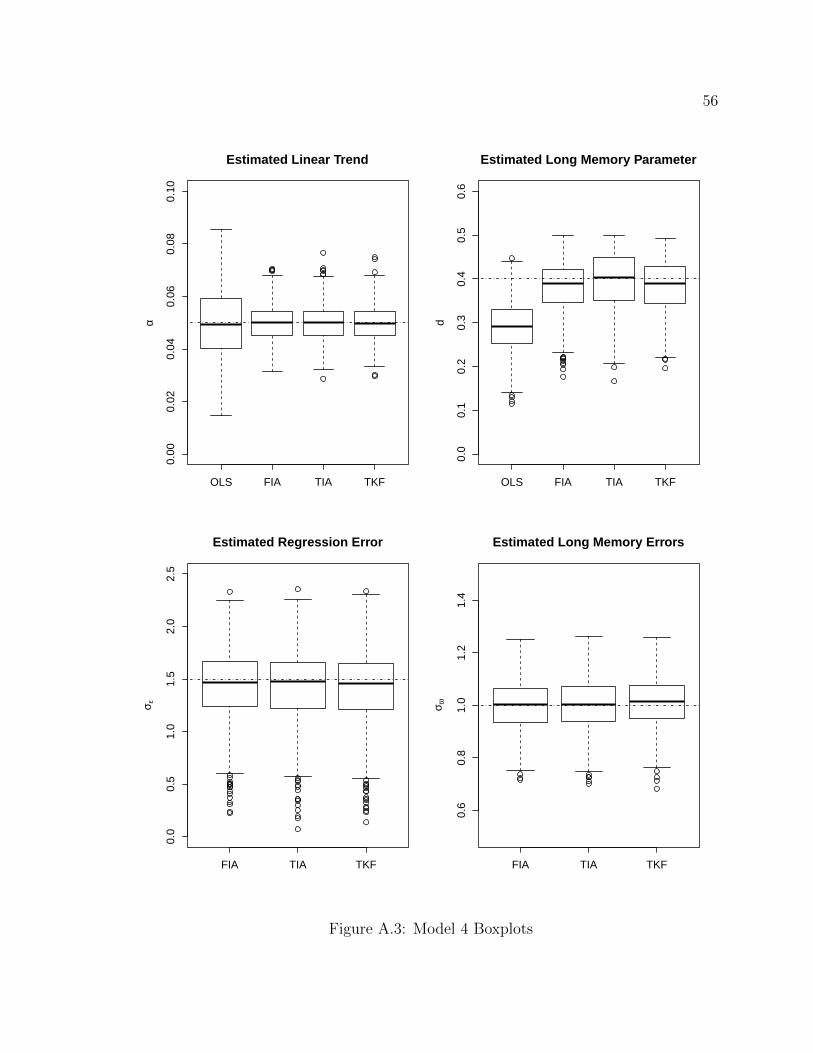
A.3 Model 4 Boxplots . . . . . . . . . . . . . . . . . . . . . . . . . . . . . . . . . . . . . . . . . . 56
A.4 Model 5 Boxplots . . . . . . . . . . . . . . . . . . . . . . . . . . . . . . . . . . . . . . . . . . 57
x

LIST OF ABBREVIATIONS
SPRM – Stochastic parameter regression model
iid – Independent and identically distributed
ARMA – Autoregressive Moving-Average
ARIMA – Autoregressive Integrated Moving-Average
ARFIMA – Autoregressive Fractionally Integrated Moving-Average
ACF – Autocorrelation function
PACF – Partial autocorrelation function
OLS – Ordinary Least-Squares
FIA – Full Innovations Algorithm
TIA – Truncated Innovations Algorithm
FKF – Full Kalman Filter
TKF – Truncated Kalman Filter
xi

LIST OF SYMBOLS
B backward shift operator; BXt = Xt−1
∇ (1−B); ∇Xt = Xt −Xt−1
Γ gamma function; Γ(α + 1) = αΓ(α) for positive α, unless otherwise noted
γ(h) Autocovariance function at lag h (for stationary series)
ρ(h) Autocorrelation function at lag h (for stationary series)
xii
1
CHAPTER 1
INTRODUCTION
1.1 Motivation
In a complex and dynamic world, the assumption that relationships in a system
remain constant is not necessarily a well-founded one. Classical time series regression
analysis assumes that the relationships between the explanatory variables and the
response variables are constant. In situations where this is not the case, applying a
classical time series regression model can lead to non-negligible errors in our predic-
tions of the response variables. Researchers in other fields have turned to modeling
situations with non-constant coefficients to explain a more dynamic relationship
between a predictor and its response. For example, changing house prices in the
United Kingdom were modeled via time-varying coefficients in [3]. For simplicity, we
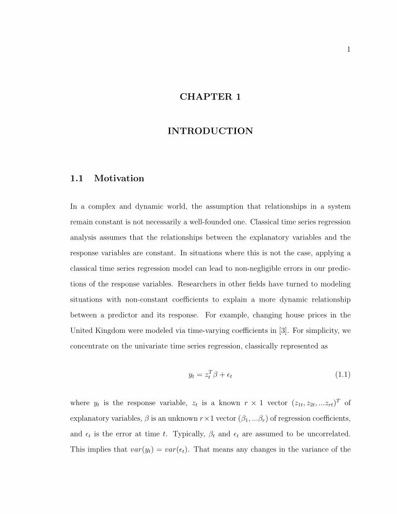
concentrate on the univariate time series regression, classically represented as
yt = zTt β + εt (1.1)
where yt is the response variable, zt is a known r × 1 vector (z1t, z2t, ...zrt)T of
explanatory variables, β is an unknown r×1 vector (β1, ...βr) of regression coefficients,
and εt is the error at time t. Typically, βt and εt are assumed to be uncorrelated.
This implies that var(yt) = var(εt). That means any changes in the variance of the

2
response is allegedly due to a change in the variance of the errors. While this may
be the case, a change in variance could also be due to a change in the relationship
between the explanatory variables and the response variable. Theoretical fixes for
non-stationary variance do exist and have been able to model some situations quite
well [7]. However, a different approach, one where changes in the variance are due to
the dynamic relationship between yt and zt, may prove more efficient and instructive.
A series, yt, is said to be stationary if its mean and autocovariance function
(ACVF), γy(h), are independent of t. That is, a stationary series has the same mean
for every time point in the series. Furthermore, a stationary series has Cov(yt, ys) =
Cov(yt+i, ys+i) for all i such that t + i, s + i ∈ 1, ..., n. In that case, we can set
h = |t − s| and say Cov(yt, ys) = Cov(yi, yi+h) = γy(h), as the covariance between
the variables depends only on the lag h = |t − s|. In other words, the relationship
between two observations only depends on how far apart they are, and not on when
they appear in the series. If γy(h) decreases very slowly, the data set is said to be
modeled by a long memory time series. More precisely, a data set is long memory if
∞∑h=−∞
|γy(h)| =∞. (1.2)
The most widely used model for long memory time series is the ARFIMA(p, d, q), or
autoregressive fractionally integrated moving-average model. The popularity of the
ARFIMA(p, d, q) model may lie in its versatility; it can approximate well any long
memory process [18] and can also account for some short memory behavior [10]. It
is also common for an ARFIMA process to have local changes in mean even though
it is stationary, which can account for otherwise inexplicable shifts in the mean of a
time series.

3
There are many different ways to account for long memory behavior in the re-
sponse variable of a time series regression. In the classical model, the long memory
component of the response is taken into account in the error series, εt. In this
case, we often model εt as an ARFIMA(p, d, q) process. This approach has been
fairly successful in economic and climatology data sets [1], [9], [12], [13], and [14].
Unfortunately, the complicated autocovariance structure of ARFIMA(p, d, q) models
presents a major difficulty with this technique. The inherent issues with analyzing
a series that is defined using a non-convergent infinite sum make more traditional
investigatory procedures challenging if not impossible. Furthermore, because a data
set can show both long memory and short memory properties, more complicated
models arise in research. One commonly used model of this type is a linear regression
with a stochastic ARMA parameter and long memory errors, discussed in Chapter 2.
However, treating long memory as part of the error series may under-emphasize the
importance of the long memory factor in the response.
1.2 Literature Review
In 1970, Thomas Burnett and Donald Gurthrie [4] developed estimators for stochastic
parameters. They found the best linear predictors that minimized the mean square
error, but they assumed that observation and explanatory variables were stationary
and that the stochastic parameter had a known covariance structure. In this paper,
we also assume that our stochastic parameter has a known covariance structure, but
relax the assumption that the observation and explanatory variables are stationary.
Given that most data sets are not stationary, this is an important improvement.
In “A Survey of Stochastic Parameter Regression” [20], Barr Rosenberg explains

4
the importance of the stochastic parameter regression models. First, he makes
the distinction between stochastic and systematic parameter processes. Systematic
parameters vary with time but are deterministic and can thus be defined by a function.
Stochastic parameters, however, are actually a realization of a process at a given time
t. Rosenberg is slightly dismissive of stochastic parameter regression models in which
the parameters are stationary time series processes, saying they are of theoretical
value, but as they cannot, in general, be written in Markovian Canonical Form,
the computational burden of these approaches is too high to be useful. A general
comparison of the OLS approach to the stochastic parameter approach is made. In
it, Rosenberg reports that inappropriate use of fixed-parameter regression results in
unbiased but highly inefficient estimation of parameters. In fact, the OLS tends to
estimate the average of the stochastic process, sometimes resulting in predictions
that are merely an average. Methods of estimation for stochastic parameters are
discussed, with the maximum likelihood estimation and Bayes Estimation being
the most commonly applied, along with the Kalman Filter estimation. Rosenberg
concludes with an example in economics illustrating how stochastic parameter models
are important; if the stochastic process itself is a meaningful quantity, then changing
relationships between predictor and response need to be more meticulously analyzed.
Newbold and Bos developed a stochastic regression model similar to the one dis-
cussed in this paper. In their paper, “Stochastic Parameter Regression Models” [17],
they regressed the quarterly inflation rate on the quarterly interest rate with the
stochastic parameter following an AR(1) process with mean b as follows:
yt = α + βtzt + νt, (1.3)
(βt − b) = φ(βt−1 − b) + ωt, (1.4)
5
where νt are iid errors. Robinson and Hidalgo [19] use this approach but generalized
it by allowing νt to have long memory. That approach is the most widely used in
modeling long memory in the response variable and is discussed further in Section 2.3.
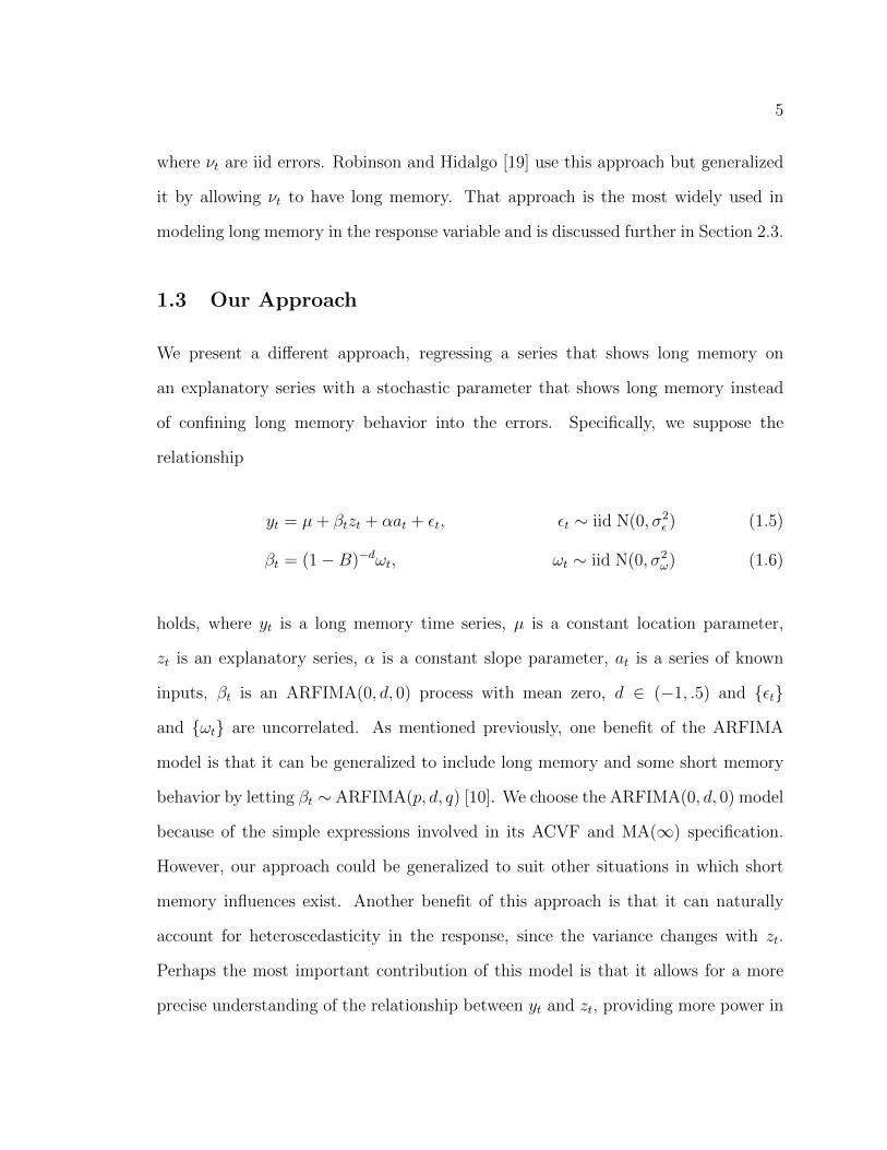
1.3 Our Approach
We present a different approach, regressing a series that shows long memory on
an explanatory series with a stochastic parameter that shows long memory instead
of confining long memory behavior into the errors. Specifically, we suppose the
relationship
yt = µ+ βtzt + αat + εt, εt ∼ iid N(0, σ2ε ) (1.5)
βt = (1−B)−dωt, ωt ∼ iid N(0, σ2ω) (1.6)
holds, where yt is a long memory time series, µ is a constant location parameter,
zt is an explanatory series, α is a constant slope parameter, at is a series of known
inputs, βt is an ARFIMA(0, d, 0) process with mean zero, d ∈ (−1, .5) and εt
and ωt are uncorrelated. As mentioned previously, one benefit of the ARFIMA
model is that it can be generalized to include long memory and some short memory
behavior by letting βt ∼ ARFIMA(p, d, q) [10]. We choose the ARFIMA(0, d, 0) model
because of the simple expressions involved in its ACVF and MA(∞) specification.
However, our approach could be generalized to suit other situations in which short
memory influences exist. Another benefit of this approach is that it can naturally
account for heteroscedasticity in the response, since the variance changes with zt.
Perhaps the most important contribution of this model is that it allows for a more
precise understanding of the relationship between yt and zt, providing more power in

6
analysis and prediction. We modify and use two previously established algorithms,
the Innovations Algorithm and the Kalman Filter, to estimate the parameters of our
model.
The rest of this paper proceeds as follows: Chapter 2 provides necessary back-
ground on time series for those less familiar with the topic, Chapter 3 explains the
details of our model, Chapter 4 discusses the Kalman Filter estimation method,
Chapter 5 discusses the Innovations Algorithm estimation method, Chapter 6 shows
a summary of simulations we performed to test the practical accuracy of the model,
and Chapter 7 contains concluding remarks.

7
CHAPTER 2
PRELIMINARY BACKGROUND
2.1 Autocorrelation
Given a series of random variables, yt, it is common to assume in introductory
statistics that the yt are independent and identically distributed. While indepen-
dence implies that two observations are not related at all, two observations being
uncorrelated implies no linear relationship. If a series is correlated with itself, it is
said to be autocorrelated. More formally, yt and ys, s 6= t, are autocorrelated if
E(ytys)−E(yt)E(ys) 6= 0. When yt and ys are correlated, E(yt|ys) 6= E(yt). Thus, if
information about the underlying autocorrelation structure of yt can be obtained,
then with observations through time t, we can use E(yt+1|yt, yt−1, ...y1) to better
predict yt+1.
Instead of assuming a series is independent or uncorrelated, time series takes
advantage of autocorrelation in a series when trying to understand how observations
are related, providing powerful prediction capabilities. One widely implemented class
of time series models is known as Autoregressive Moving-Average (ARMA) models.
Let wt, t = 1, ..., n, be an iid series. Then an ARMA(1,1) model for yt would
be yt − φyt−1 = wt + θwt−1 where φ and θ are undetermined parameters. Thus, the
observation yt depends on the observation and corresponding error from one time
point ago and the error associated with time t. If an ARMA(2,1) model were more

8
appropriate, that would suggest the observation yt depended on the observations from
two time points ago, the error from one time point ago, and the error associated with
time t. An ARMA(2,1) model reads yt − φ1yt−1 − φ2yt−2 = zt + θzt−1. The number
of parameters in an ARMA model is theoretically allowed to be any number, but in
practice a large number of parameters is frowned upon for reasons of computation,
understandability, and simplicity.
2.2 Long Memory Time Series
Long memory time series are implemented when the current observation, yt, shows
correlation with yt−k, where k takes on arbitrarily large values. One widely used
definition of a long memory time series mentioned above is
∞∑h=−∞
|γ(h)| =∞, (2.1)
where γ(h) denotes the autocovariance at lag h. This definition is a result of analyzing
long memory time series in the time domain as opposed to the frequency domain. A
popular definition of long memory used in the frequency domain treatment of time
series is
f(λ) ∼ |λ|−2dl2(1/|λ|), (2.2)
where λ is in a neighborhood of zero and l2 is a slowly varying function [18], p. 40.
This paper focuses solely on the time domain. For more information on the frequency
domain of a time series, see [2] and [18]. Qualitatively, a long memory time series is
characterized by the idea that the current observation is related to all past observa-
tions. For example, monthly inflation rates might be expected to have a long memory,

9
as the expectation of inflation can cause inflation. In fact, monthly inflation rates have
been examined in the past and found to have long memory characteristics, such as
slowly decaying autocorrelation function values [9]. Data sets with long memory occur
in a variety of other disciplines, including hydrology [11], [16] and geoscience [21].
2.2.1 ARFIMA Models
One way to model long memory time series is with an autoregressive fractionally
integrated moving-average model, ARFIMA(p, d, q), model. The ARFIMA model is
an extension of the ARMA model briefly discussed above, where p and q have the
same meaning as in the ARMA model and d is the degree of fractional differencing,
discussed below. An ARFIMA(p, d, q) model may be represented as:
φ(B)yt = θ(B)(1−B)−dωt (2.3)
where φ(B) = 1 − φ1B − ... − φpBp is the pth order autoregressive polynomial and
θ(B) = 1+θ1B+...+θqBq is the qth order moving average polynomial. The parameter
d is the long memory parameter, which describes how long of a memory the series yt
has, in some sense. We assume that φ(B) and θ(B) have no common roots. Now we
can use the binomial expansion to rewrite
(1−B)−d =∞∑j=0
ηjBj = η(B),
where
ηj =Γ(j + d)
Γ(j + 1)Γ(d)(2.4)

10
and Γ() denotes the gamma function defined as Γ(y+1) = yΓ(y) for y > 0, [21] p. 269.
The parameter d entirely determines the long memory properties of the model, so it
is important to have good estimates for d. If d = 0, the stochastic process follows
an ARMA(p, q) model. With a few additional assumptions, we have the existence a
unique stationary solution to (2.3), which is is causal and invertible.
Theorem 2.2.1. (Palma, [18]) Consider the ARFIMA process defined by (2.3). As-
sume that the polynomials φ(z) and θ(z) have no common zeros and that d ∈ (−1, 12).
Then,
(a) If the zeros of φ(z) lie outside the unit circle z : |z| = 1, then there is a unique
stationary solution of (2.3) given by
yt =∞∑
j=−∞
ϕjωt−j = ϕ(B)ωt, (2.5)
where ϕ(z) = (1− z)−dθ(z)/φ(z).
(b) If the zeros of φ(z) lie outside the closed unit disk, z : |z| ≤ 1, then the solution,
yt, is causal.
(c) If the zeros of θ(z) lie outside the closed unit disk, z : |z| ≤ 1, then the solution,
yt, is invertible.
For a proof of this theorem, see [18], p. 44. Note that if we had instead written
the ARFIMA model as φ(B)(1 − B)dyt = θ(B)ωt, the solution may no longer be
unique [18], p. 46.
From Theorem 2.2.1, we have a way to write infinite AR and infinite MA expan-
sions of the stationary, causal, and invertible solution to an ARFIMA model. For
such a solution, we have:
11
yt = (1−B)−dφ(B)−1θ(B)ωt = ϕ(B)ωt (2.6)
and
ωt = (1−B)dφ(B)θ(B)−1yt = π(B)yt. (2.7)
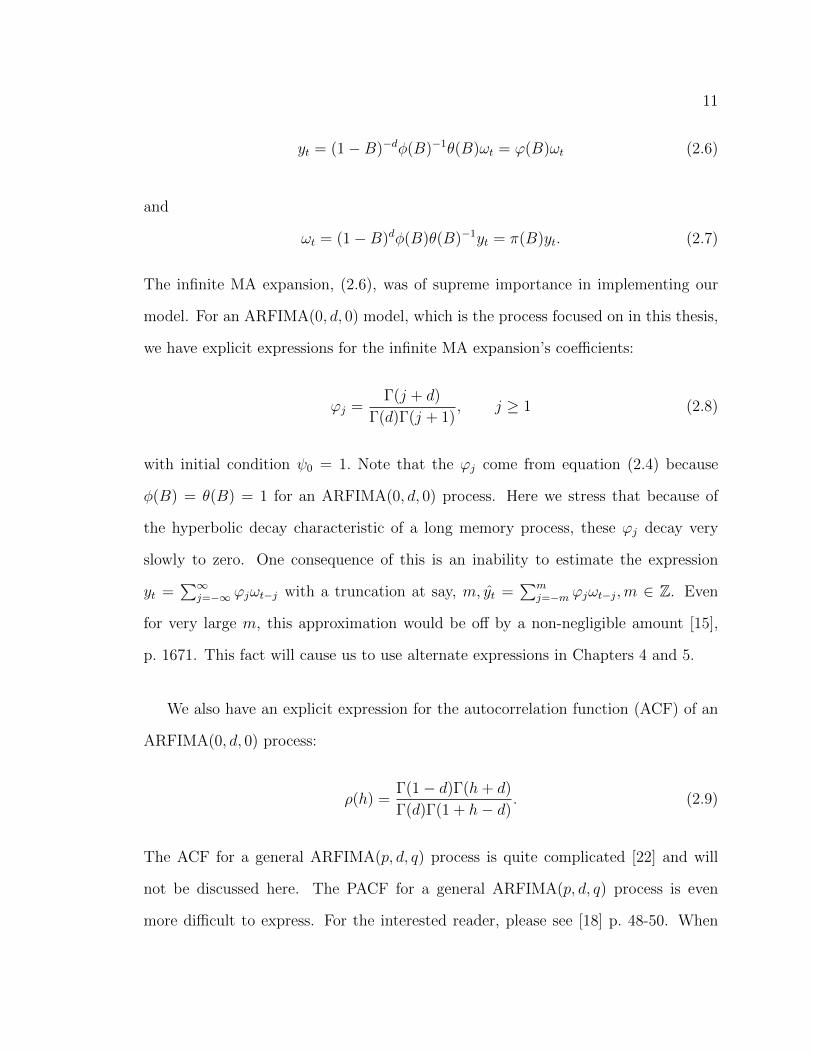
The infinite MA expansion, (2.6), was of supreme importance in implementing our
model. For an ARFIMA(0, d, 0) model, which is the process focused on in this thesis,
we have explicit expressions for the infinite MA expansion’s coefficients:
ϕj =Γ(j + d)
Γ(d)Γ(j + 1), j ≥ 1 (2.8)
with initial condition ψ0 = 1. Note that the ϕj come from equation (2.4) because
φ(B) = θ(B) = 1 for an ARFIMA(0, d, 0) process. Here we stress that because of
the hyperbolic decay characteristic of a long memory process, these ϕj decay very
slowly to zero. One consequence of this is an inability to estimate the expression
yt =∑∞
j=−∞ ϕjωt−j with a truncation at say, m, yt =∑m
j=−m ϕjωt−j,m ∈ Z. Even
for very large m, this approximation would be off by a non-negligible amount [15],
p. 1671. This fact will cause us to use alternate expressions in Chapters 4 and 5.
We also have an explicit expression for the autocorrelation function (ACF) of an
ARFIMA(0, d, 0) process:
ρ(h) =Γ(1− d)Γ(h+ d)
Γ(d)Γ(1 + h− d). (2.9)
The ACF for a general ARFIMA(p, d, q) process is quite complicated [22] and will
not be discussed here. The PACF for a general ARFIMA(p, d, q) process is even
more difficult to express. For the interested reader, please see [18] p. 48-50. When

12
investigating (2.9), we see the hyperbolic decay referenced above. In the sample ACF
of a time series, a sample correlation between the bounds ±1.96n−1/2 is said not
to be significantly different from zero. In a short memory process, the correlation
between observations decays very quickly into the insignificant range. However, for a
long memory time series, the correlations remain significant for very large time lags
because of the hyperbolic decay, contributing to the name long memory time series.
Recall that any stationary short memory time series can be modeled arbitrarily
well by an ARMA(p, q) process. Here we present the corresponding theorem for long
memory time series.
Theorem 2.2.2. (Palma, [18]) Let yt : t ∈ Z be a linear regular process satisfying
yt =∑∞
j=0 ψjεt−j = ψ(B)εt, where ψ0 = 1 and∑∞
j=1 ψ2j < ∞ with strictly positive
spectral density fy satisfying f(λ) ∼ |λ|−2df2(|λ|). Then, there exists an ARFIMA
process with spectral density f such that for any ε > 0,
∣∣∣∣fy(λ)
f(λ)− 1
∣∣∣∣ < ε,
uniformly for λ ∈ [−π, π].
Because this theorem is proved in the frequency domain, it requires more back-
ground for understanding than provided here, so interested readers may find the proof
in [18], p. 55.

13
2.3 Linear Regression with Autocorrelated Errors
Recall that the classical univariate linear model is of the form (1.1). It is common to
suppose that εt is iid. However, in many cases, this is an inappropriate assumption.
Indeed, if there is autocorrelation in the error, we may be able come up with better
predictions. Thus, models arose assuming εt was an ARMA and more recently an
ARFIMA process. The estimation procedure usually uses the least-squares approxi-
mation for β and fits an ARMA or ARFIMA model to the sample residuals. Then,
β can be re-estimated after subtracting the fitted values from yt. This procedure
is repeated until the estimates converge. As mentioned previously, this is the most
common approach when long memory is apparent in yt. However, note that in this
case, var(yt) = var(εt), implying that any change in the variance of the response
series is due to fluctuation in the error. While this may be true in some cases,
it also makes sense that variation in the response should be linked to variance in
the explanatory series. One answer to this problem is to suppose that β is in fact
a stochastic process instead of a constant. If the series shows both long memory
and short memory characteristics, βt might be modeled as an ARMA process with
ARFIMA errors. A model supposing βt is long memory does not appear to have
occurred in the literature, and will be explained in the next chapter.
2.4 Maximum Likelihood Estimation
Maximum likelihood estimation, or MLE, is a widely used method of estimation in
statistics. The idea behind the MLE is that given a family of distribution functions
with a vector of parameters θ, we find the most likely value of θ given a set of
observations, y1, ..., yn. An example taken from “Mathematical Statistics with
14
Applications,” [23], is as follows: suppose we choose two balls from a box containing
three balls with color red or white. We do not know how many balls are red and
white, but we choose two red balls without replacement. We know that the number
of red balls in the box must have been two or three. If there are only two red balls,
the probability of choosing those two balls is
(2
2
)(1
0
)(
3
2
) =1
3.
However, if the number of red balls is actually three, then the probability of choosing
two red balls from three red balls is one! Since it is much more likely that there are
three red balls, given the random sample, we would hypothesize that the number of
red balls is three. This is an intuitive example of the maximum likelihood logic. A
more formal definition of maximum likelihood is given below.
Definition 2.4.1. : Method of Maximum Likelihood [23] p. 477
Suppose that the likelihood function depends on k parameters θ1, ..., θk. Choose as esti-
mates those values of the parameters that maximize the likelihood L(y1, ..., yn|θ1, ..., θk).
If the random sample consists of continuous random variables, then the likelihood
function L(θ) is the joint density function of those random variables. Since ln(L(θ)),
known as the log-likelihood function, is a monotonically increasing function of L(θ),
ln(L(θ)) is maximized when L(θ) is maximized. The log-likelihood function has some
nice properties in regards to numerical stability and derivative calculation and is
therefore often used in practice instead of the likelihood function.

15
CHAPTER 3
STOCHASTIC PARAMETER REGRESSION FOR LONG
MEMORY TIME SERIES
3.1 Model Specification
We would like to develop a model where the long memory component is not treated as
a random accident, but an integral component of the series in question. To that end,
we suppose that given an explanatory series, zt, and a long memory response series,
yt, the relationships (1.5) and (1.6) hold. Because we have specified βt to follow an
ARFIMA(0, d, 0) process, we are only concerned with a series βt that is fractionally
integrated white noise, but our approach could be generalized to an ARFIMA(p, d, q)
process in order to model both long and short memory characteristics. Our approach
allows εt to take its classic linear regression role as iid errors. Note that the variance
of yt depends on the values of zt and the variance of βt as follows:
var(yt) = var(µ) + var(ztβt) + var(αat) + var(εt) (3.1)
= z2t var(βt) + σ2
ε = z2t σ
2ω + σ2
ε . (3.2)
Thus, as zt increases, the variance of yt increases. This gives more explanatory power
to zt and contributes to a better understanding of the behavior of yt.
One example where large zt values might contribute to more variance in yt is

16
large inflation values on nominal interest rates. In the late 1970s, inflation had
increased so much that the Federal Reserve made a sharp increase in interest rates
to encourage deflation. Doing so caused much unrest in the economy, and given the
different opinions over the effects of high inflation inside the Federal Reserve, interest
rates might have decreased much more quickly, causing even more fluctuation than
was seen at the time. As it was, the Federal Reserve still adjusted interest rates a
considerable amount until inflation broke. In times where the economy is not under
such duress, the inflation rate is under control and the Federal Reserve keeps interest
rates relatively constant. That is, when inflation is high, it causes interest rates to
be more variable. We plot this data set in Figure 3.1, using rates on three month
Treasury bills as a measure of interest rates. This data set is not appropriate for our
model as interest rates do not seem to display long memory, but the historical data
supports the hypothesis that large inflation rates contribute to more variable interest
rates. A plot of this data is shown in Figure 3.1. The data came from [6] and [8]. This
example demonstrates the need for stochastic parameter regression models because
of the increased variability of yt for different values of zt.
A pictorial example of a data set that could be well-explained by our model is
shown in Figure 3.2 and Figure 3.3. Figure 3.2 shows the yt and zt time series plots
on the same graph. The yt series has an intercept around ten and the zt series
has an intercept close to zero. Note that for peaks in zt values, yt tends to be
more variant. Furthermore, yt appears to have local changes in mean, something
the ARFIMA(0, d, 0) model accounts for. Figure 3.3 shows a scatterplot of yt and
zt. Notice that the variance of yt increases for large values of zt. This is because
the variance of yt is dependent on the values of zt. Because we take E(βt) = 0, the
scatterplot is centered at zero. This particular series was generated by taking zt to

17
0 5 10 15 20
05
1015
Quarterly Interest Rates On Inflation
Inflation
3 M
onth
Tre
asur
y B
ills
Figure 3.1: Interest Rates on Inflation
be a linear trend with AR(1) errors. That is, zt = α0 +α1t+ ξt, where ξt = φξt−1 + ηt
and ηt ∼ iid N(0, σ2η). We let α0 = 0, α1 = .05, φ = .8 and σ2
η = 1. We also set µ = 10,
α = 0, σε = 1.5 and σω = 1. Here, βt is generated from a zero-mean ARFIMA(0, d, 0)
process with d = .4. Notice that at first glance, it may not be obvious that yt and
zt are linearly related. This means that data that should be theoretically related but
do not appear to be so in practice may be explained by a model similar to ours. We
definitely notice heteroscedasticity, with larger variance for larger values of zt. In
summary, our model has the flexibility to take into account long memory influences
in a time series, like local changes in mean, and is able to explain increasing variance
for larger values of the explanatory variable.

18
Time
y.t
0 50 100 150 200
−5
05
1015
20
Figure 3.2: Simulated Time Series Plot
−1 0 1 2 3
510
15
z.t
y.t
Figure 3.3: Simulated Scatterplot

19
3.2 Estimation Methods
In the next two chapters, we introduce our modifications to the Kalman Filter and
Innovations Algorithm, which allow us to use maximum likelihood estimation for our
parameters. We have four different techniques: a full Kalman Filter, a truncated
Kalman Filter, a full Innovations Algorithm, and a truncated Innovations Algorithm.
The maximum likelihood function has been investigated for these methods, so we can
adapt maximum likelihood estimation to our purposes.
One extension of the likelihood function is Whittle Estimation, often used to
estimate parameters when the observations show long memory and sometimes used
by built-in estimation routines in statistical programs [2], p. 363. Whittle Estimation
is a frequency domain approach and is a result of the fact that calculating the exact
likelihood function of an ARFIMA process is computationally demanding. However,
Whittle Estimation will not be used here as Chan and Palma [5] came up with another
way around using the exact likelihood function for estimation:
Theorem 3.2.1. (Chan and Palma, [5], Theorem 2.2)
Let y1, ..., yn be a finite sample of an ARFIMA(p, d, q) process. If Ω1 is the variance
of the initial state X1 for the infinite-dimensional representation, then the computa-
tion of the exact likelihood function depends only on the first n components of the
Kalman equations.
In other words, we can obtain the exact likelihood function for an ARFIMA process
with a finite sample of n. For the proof, see [5]. This approach is what we use in
our estimation methods. Because we have assumed that εt and ωt are Gaussian
processes, maximum likelihood estimation holds theoretical merits for estimating the
parameters of our model. We then use the expressions derived below to obtain the

20
innovations for each method and use those innovations to compute the maximum
likelihood function. Each likelihood function shown is equivalent, but the different
forms are included for notation purposes. We then use a Newton-Raphson procedure
with the “optim” function from R to obtain maximum likelihood estimates. For the
rest of the paper, we will suppose that the response variable yt and the covariate zt
have the relationship defined in (1.5) and (1.6).

21
CHAPTER 4
THE KALMAN FILTER
The Kalman Filter uses a state space representation to obtain the prediction expres-
sion with minimum mean square error in the class of linear estimators [21], p. 325.
The Kalman Filter is a special application of state space models, so before presenting
the Kalman Filter, it would be prudent to begin with a discussion of said state space
models.
4.1 State Space Representation
State space models, also known as Dynamic Linear Models, are based on the premise
that the random variable of interest, the state variable, is not directly observed;
rather, we observe some linear combination of the state variable plus noise. The
basic observation equation is
yt = GtXt + εt, (4.1)
and the state equation is
Xt = FXt−1 +Wt. (4.2)
We assume that Wt ∼ iid N(0, Q) and εt ∼ iid N(0, R). While it is not a necessary
assumption, we keep things simple by supposing that Wt and εt are independent.
We also assume that X0 ∼ N(µ0,Ω0). Here, Xt and Wt are p×1 vectors, Ft is a p×p

22
matrix, yt and εt are q × 1 vectors, Gt is q × p matrix, and q is allowed to be less
than, equal to, or greater than p. For the purpose of broadening the model, we can
also include inputs in the basic state and observation equation in the following way:
yt = GtXt + Γut + εt, (4.3)
Xt = FXt−1 + ζut +Wt. (4.4)
At first glance, the requirement that the state variable be well-fitted by an AR(1)
model may seem ill-suited to many situations. However, the state equation actually
allows for great flexibility. For example, in the univariate case, suppose we wish to
measure state βt, which is actually better fitted by an AR(m) model. We may then
write the state equation in the following way:
βt
βt−1
...
βt−m+1
=
φ1 φ2 · · · φm
1 0 0 0
.... . . . . .
...
0 · · · 1 0
βt−1
βt−2
...
βt−m
+
ωt
0
...
0,
, (4.5)
where Xt = (βt, βt−1, ..., βt+m−1)T . The observation equation becomes
yt =
[Gt 0 · · · 0
]Xt + εt. (4.6)
In our case, we wish to measure the ARFIMA(0, d, 0) state βt, which follows an
AR(∞) model, specified in Theorem 2.2.1. It may be apparent to careful readers
that we would need an infinite state space model for our case. That intuition is
correct, as confirmed by Chan and Palma in [5], but we will demonstrate a way

23
around this issue in Section 4.3. For more details on state space models, see [21].
With this groundwork laid out, we will consider the Kalman Prediction Equations.
4.2 Kalman Prediction
The Kalman Filter prediction equations are as follows:
Theorem 4.2.1. (Shumway and Stoffer, [21]) For the state-space model specified in
(4.3) and (4.4), with initial conditions E(X0) = µ0 and var(X0) = Ω0, the Kalman
prediction equations are:
Xt|t−1 = FtXt−1|t−1 + ζut,
Ωt|t−1 = FtΩt−1|t−1FTt +Q,
Xt|t = Xt|t−1 +Kt(yt −GtXt|t−1 − Γut),
Ωt|t = [I −KtGt]Ωt|t−1,
where I is the identity matrix and
Kt = Ωt|t−1GTt [GtΩt|t−1G
Tt +R]−1.
Kt is called the Kalman gain and is, in some sense, a measure of how well Xt|t−1
actually predicted Xt|t [21]. In addition to these equations, we also calculate the
corresponding innovations, which will be used to calculate the maximum likelihood
estimate. The innovations are:
υt = yt − E(yt|yt−1, yt−2, ...) = yt −GtXt|t−1 − Γut, (4.7)
24
and their corresponding variance-covariances matrices are:
Σt = var(yt −Gtxt|t−1 − Γut) = var(GtXt + εt −GtXt|t−1) = GtΩt|t−1GTt +R. (4.8)
These innovations are uncorrelated, which allows us to use them for the innovations
form of the maximum likelihood function, discussed below. As previously mentioned,
the Kalman estimates are those with the minimum mean square error in the class
of linear estimators. Another advantage of the Kalman equations is that once we
have calculated Xt|t−1, we can use that and yt to calculate Xt+1|t instead of having
to recalculate all the estimates over again. This makes the Kalman equations very
useful for real-time data. The final advantage is a bit more specific to this paper; the
Kalman Prediction equations give us expressions for the conditional expectation of
βt, which is useful for prediction purposes.
4.3 Full Kalman Filter
We would like to find the Kalman Prediction expressions for our model, represented
in (1.5) and (1.6). This presents a challenge; in 1998, Chan and Palma [5] proved that
there is no finite dimensional state space model for a long memory ARFIMA process.
However, we can extract the exact likelihood function of a long memory process from
a finite dimensional expression following Chan and Palma’s approach [5], by way of
Theorem 3.2.1 from Chapter 3.
Note that, in our notation, Ω1 is called Ω0|0 and X1 = X0|0. Furthermore, because
our state space equations are different from those in [5], the likelihood actually
depends on the first n+1 equations. Therefore, if our state space model is accurate for

25
the first n+1 rows, our likelihood function should be exact. To use Theorem 3.2.1, we
will first state and prove a lemma used in the specification of our state space model.
Lemma 4.3.1. Let βt be a zero-mean stationary ARFIMA(0, d, 0) process with
d ∈ (−1, 0.5). For i = 1, . . . ,m, we have
βt+i|t =∞∑k=i
ϕkωt+i−k.
Proof. We will prove this for i = 1. Since βt = (1 − B)−dωt =∑∞
k=0 ϕkωt−k with
ϕk = Γ(k+d)Γ(d)Γ(k+1)
, we have
βt+1|t = E(βt+1|βt, βt−1, · · · )
= E
(∞∑k=0
ϕkωt+1−k
∣∣∣∣βt, βt−1, · · ·
)
= E(ωt+1|βt, βt−1, · · · ) + E
(∞∑k=1
ϕkωt+1−k
∣∣∣∣βt, βt−1, · · ·
)
=∞∑k=1
ϕkωt+1−k
because E(ωt+1|βt, βt−1, · · · ) = E(ωt+1) = 0 and E(∑∞
k=1 ϕkωt+1−k|βt, βt−1, · · · ) =∑∞k=1 ϕkωt+1−k, as
∑∞k=1 ϕkωt+1−k only involves data from the first t observations.
Now we specify a new state space specification used for our model. We define the
observation and state equations (4.3) and (4.4) as follows:
Theorem 4.3.2. The state space representation (4.3) and (4.4) correctly models (1.5)
and (1.6), where

26
Xt =
βt
βt+1|t
...
βt+n|t
, F =
0 1 0 0 · · · 0
0 0 1 0 · · · 0
0 0 0 1 · · · 0
......
.... . . . . .
...
0 0 0 0 · · · 1
0 0 0 0 · · · 0
,Wt =
1
ϕ1
...
ϕn
ωt, Gt =
[zt 0 · · · 0
].
Here, βt+i|t = E(βt+i|βt, βt−1, ...) and Wt ∼ iid N(0, Q) where
Q = σ2ω
1 ϕ1 · · · ϕn
ϕ1 ϕ21 · · · ϕ1ϕn
......
. . ....
ϕn ϕnϕ1 · · · ϕ2n
If there is a drift in the data of α, then we set Γ =
[µ α
]and ut =
1
t
. Otherwise,
Γ = µ and ut = 1. Now, assume X0 ∼ N(X0|0,Ω0|0). We set X0|0 = 0 since E(βt) = 0
and have
Ω0|0 =
γβ(0) γβ(1) · · · γβ(n)
γβ(1)
... T
γβ(n)
(4.9)
where γβ(h) is the ACVF of βt, and the n× n matrix T has
Tij =
γβ(j − i)− σ2ω
∑i−1k=0 ϕkϕk+(j−i), i ≤ j
Tji, i > j(4.10)

27
Proof. First, we will show that (4.3) and (4.4) are equivalent to (1.5) and (1.6).
Showing the equivalence of (1.5) and (4.3) is straightforward as GtXt = βtzt. Now
we focus on the state equation, (4.4). For this, note that the state equation (4.4) is
equivalent to the following system of equations:
βt = βt−1+1|t−1 + ωt,
βt+1|t = βt−1+2|t−1 + ϕ1ωt,
...
βt+n−1|t = βt−1+n|t−1 + ϕn−1ωt,
βt+n|t = ϕnωt.
We will show the first n equations hold true. For this, we use Lemma 4.3.1 to obtain:
βt =∞∑k=0
ϕkωt−k = ωt +∞∑k=1
ϕkωt−k = ωt +∞∑k=1
ϕkωt−1+1−k = ωt + βt−1+1|t−1,
which is equivalent to the first equation above. Next, Lemma 4.3.1 gives, for i =
1, . . . , n− 1,
βt+i|t =∞∑k=i
ϕkωt+i−k
= ϕiωt +∞∑
k=i+1
ϕkωt−1+i+1−k
= ϕiωt + βt−1+i+1|t−1,
which corresponds to the second through nth equations. The last equation is not
true, but for large n, this would be appreciably negligible as shown in [5].

28
Now, for the initial condition on Ω0|0 in (4.9), note that the stationarity of Xt
gives
Ω0|0 = V ar(X0)
= V ar(Xt)
=
V ar(βt) Cov(βt, βt+1|t) · · · Cov(βt, βt+n|t)
Cov(βt+1|t, βt) V ar(βt+1|t) · · · Cov(βt+1|t, βt+n|t)
......
. . ....
Cov(βt+n|t, βt) Cov(βt+n|t, βt+1|t) · · · V ar(βt+n|t)
.
First, we consider the following covariances: for j = 1, . . . , n,
Cov(βt, βt+j|t) = Cov
(∞∑k=0
ϕkωt−k,∞∑k=j
ϕkωt+j−k
)
= σ2ω
∞∑k=0
ϕkϕk+j
= σ2ω
∞∑k=0
Γ(k + d)
Γ(d)Γ(k + 1)
Γ(k + j + d)
Γ(d)Γ(k + j + 1)
= σ2ω
Γ(j + d)
Γ(d)Γ(j + 1)
∞∑k=0
Γ(k + d)Γ(k + j + d)Γ(j + 1)
Γ(k + 1)Γ(d)Γ(j + d)Γ(k + j + 1)
= σ2ω
Γ(j + d)
Γ(d)Γ(j + 1)F (d, j + d; j + 1; 1)
= σ2ω
Γ(j + d)
Γ(d)Γ(j + 1)
Γ(j + 1)Γ(1− 2d)
Γ(j + 1− d)Γ(1− d)
= γβ(j).
Here, F (x, y; v;w) is the hypergeometric function. Second, consider, for i ≤ j, i, j =
1, . . . , n,

29
τi,j = Cov(βt+i|t, βt+j|t)
= Cov
(∞∑k=i
ϕkωt+i−k,∞∑k=j
ϕkωt+j−k
)
= σ2ω
∞∑k=i
ϕkϕk+(j−i)
= σ2ω
(∞∑k=0
ϕkϕk+(j−i) −i−1∑k=0
ϕkϕk+(j−i)
)
= γβ(j − i)− σ2ω
i−1∑k=0
ϕkϕk+(j−i).
These results verify our expression of Ω0|0 in (4.9).
Now that we have expressions for the innovations from the Kalman Filter, we use
these innovations to compute the likelihood function:
L(µ, α, σε, d, σω) = (2π)−n/2
(n∏j=1
det Σt
)−1/2
exp
[−1
2
n∑j=1
υTt Σ−1t υt
]. (4.11)
Since, in our case, Σt and νt are scalars, this makes the log-likelihood function:
`(µ, α, σε, d, σω) = L(µ, α, σε, d, σω) = −1
2
n∑j=1
ln Σt −1
2
n∑j=1
υ2t
Σt
. (4.12)
when the constant term in (4.11) is ignored. This is also the likelihood function
expression for the Truncated Kalman Filter, detailed in the next section.
4.4 Truncated Kalman Filter
Thus far, we have developed a state space model of dimension (n + 1) × (n + 1).
In comparison to an infinite dimensional state space model, this is good news for
30
computer estimation. However, using the Full Kalman Filter method described above
can be cumbersome for large n. One might be tempted to simply cut off the Full
Kalman Filter expressions, but because of the nature of a long memory time series,
simply cutting off the MA(∞) expression leads to non-negligible errors, as discussed
in Chapter 2. To that end, we would like to introduce a Truncated Kalman Filter of
dimension m×m where m is considerably less than n. For that purpose, we turn our
attention to the series δt = βt − βt−1.
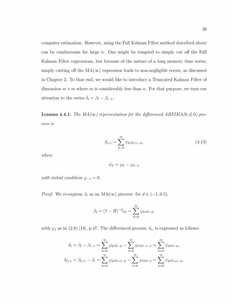
Lemma 4.4.1. The MA(∞) representation for the differenced ARFIMA(0, d, 0) pro-
cess is
δt+i =∞∑k=0
ψkωt+i−k, (4.13)
where
ψk = ϕk − ϕk−1
with initial condition ϕ−1 = 0.
Proof. We re-express βt as an MA(∞) process: for d ∈ (−1, 0.5),
βt = (1−B)−dωt =∞∑k=0
ϕkωt−k,
with ϕj as in (2.8) [18], p.47. The differenced process, δt, is expressed as follows:
δt = βt − βt−1 =∞∑k=0
ϕkωt−k −∞∑`=0
ϕ`ωt−1−` =∞∑k=0
ψkωt−k,
δt+1 = βt+1 − βt =∞∑k=0
ϕkωt+1−k −∞∑`=0
ϕ`ωt−` =∞∑k=0
ψkωt+1−k,
31
where ψk = ϕk − ϕk−1 with the initial condition ϕ−1 = 0. In general, we can deduce
(4.13): for i = 0, 1, . . .,
δt+i =∞∑k=0
ψkωt+i−k,
which is an MA(∞) representation for the differenced process δt+i = βt+i−βt+i−1.
One of the solutions Chan and Palma [5] came up with for the problem of being
unable to write a finite state space model was to consider the differenced series.
Indeed, since ψk → 0 faster than ϕk → 0, Chan and Palma truncate this expression
after m. That is,
δt+i ≈m∑k=0
ψkωt+i−k (4.14)
Lemma 4.4.2. The conditional expectation of δt+i given βt, ..., β1 has the expression
δt+i|t = E(δt+i|βt, ..., β1)
≈m∑k=i
ψkωt+i−k
Proof. We consider the conditional expectation of the differenced process δt as
follows. Using the MA(∞) expression (4.13) and the MA(m) truncation expression
(4.14), we obtain:

32
δt+1|t = E
(∞∑k=0
ψkωt+1−k
∣∣∣∣βt, βt−1, · · ·
)
≈ E
(m∑k=0
ψkωt+1−k
∣∣∣∣βt, βt−1, · · ·
)
= E(ωt+1|βt, βt−1, · · · ) + E
(m∑k=1
ψkωt+1−k
∣∣∣∣βt, βt−1, · · ·
)
=m∑k=1
ψkωt+1−k,
δt+2|t = E
(∞∑k=0
ψkωt+2−k
∣∣∣∣βt, βt−1, · · ·
)
≈ E
(m∑k=0
ψkωt+2−k
∣∣∣∣βt, βt−1, · · ·
)
= E(ωt+2) + ψ1E(ωt+1) + E
(m∑k=2
ψkωt+2−k
∣∣∣∣βt, βt−1, · · ·
)
=m∑k=2
ψkωt+2−k,
which inductively results in the truncated expression in Lemma 4.4.2.
If we suppose that m in the approximation equation is such that (4.14) is within
a reasonable margin of error, we will take
δt+i =m∑k=0
ψkωt+i−k
From Lemma 4.4.2, we get:
δt−1+i|t−1 ≈m∑k=i
ψkωt−1+i−k (4.15)
Now we will present our long memory SPR model via the following truncated
33
state space model representation.
Theorem 4.4.3. The state space representation (4.3) and (4.4) correctly models (1.5)
and (1.6), where
Xt =
βt
δt+1|t
...
δt+m|t
, F =
1 1 0 0 · · · 0
0 0 1 0 · · · 0
0 0 0 1 · · · 0
......
.... . . . . .
...
0 0 0 0 · · · 1
0 0 0 0 · · · 0
,Wt =
1
ψ1
...
ψm
, Gt =
[zt 0 · · · 0
].
Here, Wt ∼ iid N(0, Q) with
Q = σ2ω
1 ψ1 · · · ψm
ψ1 ψ21 · · · ψ1ψm
......
. . ....
ψm ψmψ1 · · · ψ2m
.
We now assume that X0 ∼ N(x0|0,Ω0|0). Since E(βt) = 0, we find X0|0 = 0 and
Ω0|0 =
σ2ω
Γ(1−2d)Γ(1−d)2
σ2ω
∑m−1k=0 ϕkψk+1 · · · σ2
ωϕ0ψm
σ2ω
∑m−1k=0 ϕkψk+1
... T
σ2ωϕ0ψm
,
where T is an m×m matrix with
34
Tij =
σ2ω
∑m−1k=i ψkψk+(j−i), i ≤ j;
Tji, i > j.
Proof. First we will show that (4.3) and (4.4) are equivalent to (1.5) and (1.6).
Showing the equivalence of (1.5) and (4.3) is straightforward as GtXt = βtzt. Now
we focus on the state equation, (4.4). For this, note that the state equation (4.4) is
equivalent to the following system of equations:
βt = βt−1 + δt|t−1 + ωt,
δt+1|t = δt−1+2|t−1 + ψ1ωt,
...
δt+m−1|t = δt−1+m|t−1 + ψm−1ωt,
δt+m|t = ψmωt.
We will show these m+ 1 equations hold true (within an approximation of m). First,
we use (4.13) and (4.15) as follows:
βt − βt−1 = δt ≈m∑k=0
ψkωt−k = ωt +m∑k=1
ψkωt−1+1−k = ωt + δt−1+1|t−1,
which is equivalent to the first equation above. Second, we use Lemma 4.4.2 to obtain,
for i = 1, . . . ,m− 1,
δt+i|t ≈m∑k=i
ψkωt+i−k = ψiωt +m∑
k=i+1
ψkωt−1+i+1−k = ψiωt + δt−1+i+1|t−1,
which corresponds to the second through mth equations. Last, using Lemma 4.4.2

35
gives
δt+m|t ≈m∑
k=m
ψkωt+m−k = ψmωt
as required in the (m+ 1)th equation of (4.4).
Now we will show that the expression of Ω0|0 is correct. Because Xt is stationary,
we have that
Ω0|0 = V ar(X0)
= V ar(Xt)
=
V ar(βt) Cov(βt, δt+1|t) · · · Cov(βt, δt+m|t)
Cov(δt+1|t, βt) V ar(δt+1|t) · · · Cov(δt+1|t, δt+m|t)
......
. . ....
Cov(δt+m|t, βt) Cov(δt+m|t, δt+1|t) · · · V ar(δt+m|t)
.
We also know that the stationary ARFIMA(0, d, 0) process βt has variance
V ar(βt) = γβ(0) = σ2ω
Γ(1− 2d)
Γ(1− d)2,
which verifies the (1, 1)th element of Ω0|0. From Lemma 4.4.2 and the infinite MA
expansion of βt, we have
Cov(βt, δt+j|t) ≈ Cov
(∞∑k=0
ϕkωt−k,m∑k=j
ψkωt+j−k
)
= σ2ω
m−j∑k=0
ϕkψk+j,
for j = 1, . . . ,m, which verifies the remaining elements in the first row of Ω0|0. Finally,
for i ≤ j, we have
36
Ti,j = Cov(δt+i|t, δt+j|t)
≈ Cov
(m∑k=i
ψkωt+i−k,m∑k=j
ψkωt+j−k
)
= σ2ω(ψiψi+(j−i) + ψi+1ψi+1+(j−i) + · · ·+ ψm−(j−i)ψm−(j−i)+(j−i))
= σ2ω
m−(j−i)∑k=i
ψkψk+(j−i),
which verifies the expression for T .

37
CHAPTER 5
THE INNOVATIONS ALGORITHM
The Innovations Algorithm and the Durbin-Levinson Algorithm are both one-step
prediction recursion schemes. The Durbin-Levinson Algorithm can have smaller
variance, but has the requirement that the series it is predicting be stationary. The
Innovations Algorithm, however, only requires the series have a finite second moment,
meaning it can be applied directly to a non-stationary series. This is important
because one of the advantages of our model is the ability to take into account dynamic
variance patterns. Thus, the technique used to predict the series must also not require
stationarity.
5.1 Best Linear Predictor
The Innovations Algorithm stems from applications of the best linear predictor. The
best linear predictor of random variable is defined as the linear combination of past
values that has minimum variance [2], p. 63. If we denote the best linear predictor
of Xn+h given n past values as PnXn+h, then the best linear predictor of a stationary
time series given X1, X2, ..., Xn is
PnXn+h = µ+n∑i=1
ai(Xn+1−i − µ), (5.1)
38
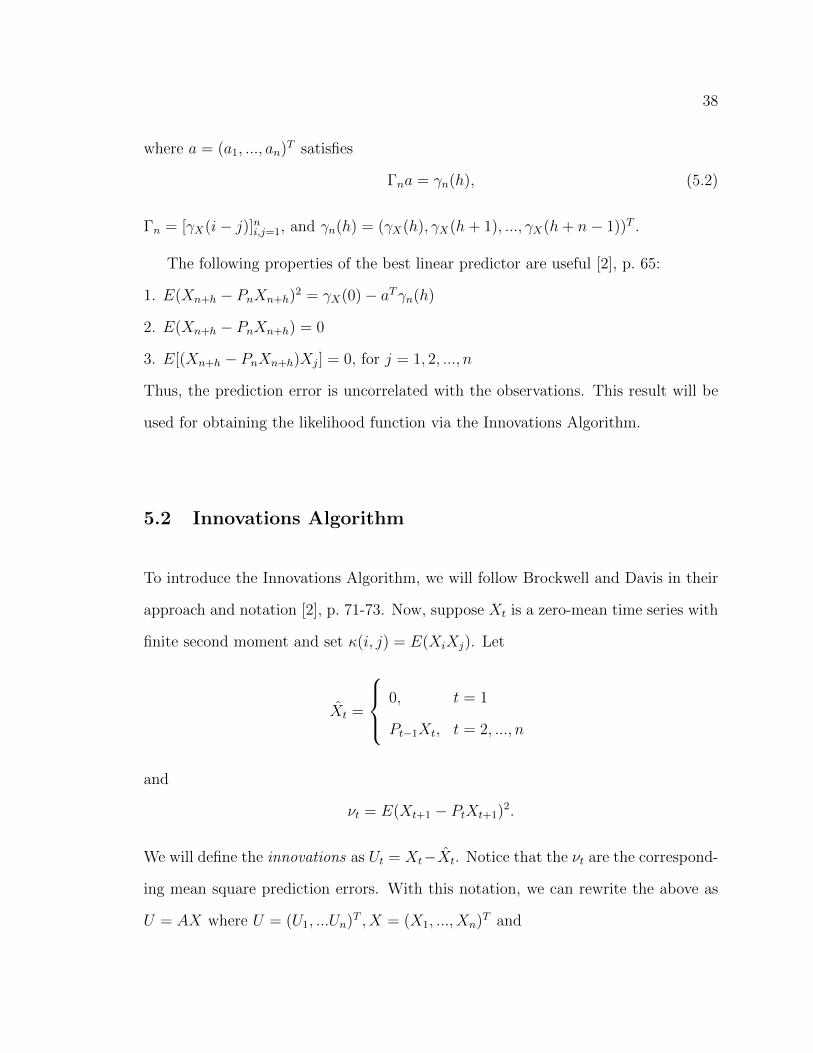
where a = (a1, ..., an)T satisfies
Γna = γn(h), (5.2)
Γn = [γX(i− j)]ni,j=1, and γn(h) = (γX(h), γX(h+ 1), ..., γX(h+ n− 1))T .
The following properties of the best linear predictor are useful [2], p. 65:
1. E(Xn+h − PnXn+h)2 = γX(0)− aTγn(h)
2. E(Xn+h − PnXn+h) = 0
3. E[(Xn+h − PnXn+h)Xj] = 0, for j = 1, 2, ..., n
Thus, the prediction error is uncorrelated with the observations. This result will be
used for obtaining the likelihood function via the Innovations Algorithm.
5.2 Innovations Algorithm
To introduce the Innovations Algorithm, we will follow Brockwell and Davis in their
approach and notation [2], p. 71-73. Now, suppose Xt is a zero-mean time series with
finite second moment and set κ(i, j) = E(XiXj). Let
Xt =
0, t = 1
Pt−1Xt, t = 2, ..., n
and
νt = E(Xt+1 − PtXt+1)2.
We will define the innovations as Ut = Xt−Xt. Notice that the νt are the correspond-
ing mean square prediction errors. With this notation, we can rewrite the above as
U = AX where U = (U1, ...Un)T , X = (X1, ..., Xn)T and
39
A =
1 0 0 · · · 0
a11 1 0 · · · 0
a22 a21 1 · · · 0
......
.... . . 0
an−1,n−1 an−1,n−2 an−1,n−3 · · · 1
.
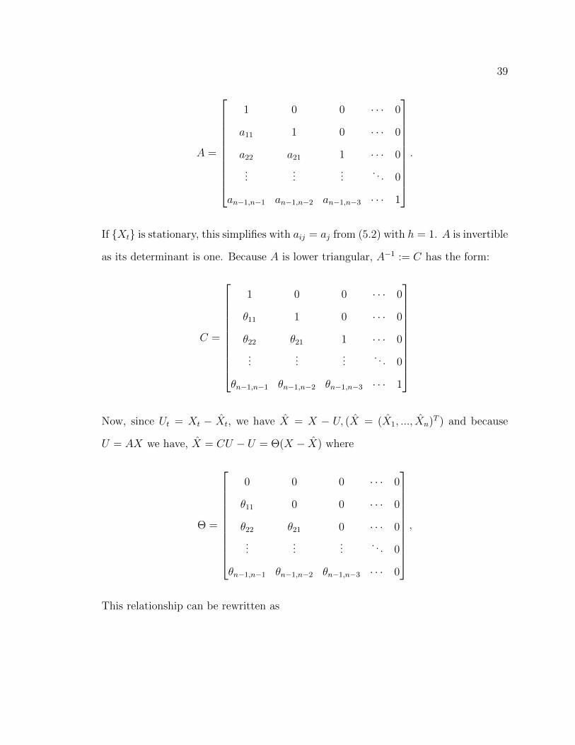
If Xt is stationary, this simplifies with aij = aj from (5.2) with h = 1. A is invertible
as its determinant is one. Because A is lower triangular, A−1 := C has the form:
C =
1 0 0 · · · 0
θ11 1 0 · · · 0
θ22 θ21 1 · · · 0
......
.... . . 0
θn−1,n−1 θn−1,n−2 θn−1,n−3 · · · 1
Now, since Ut = Xt − Xt, we have X = X − U, (X = (X1, ..., Xn)T ) and because
U = AX we have, X = CU − U = Θ(X − X) where
Θ =
0 0 0 · · · 0
θ11 0 0 · · · 0
θ22 θ21 0 · · · 0
......
.... . . 0
θn−1,n−1 θn−1,n−2 θn−1,n−3 · · · 0
,
This relationship can be rewritten as

40
Xt+1 =
0, t = 0∑nj=1 θtj(Xt+1−j − Xt+1−j), t = 1, ..., n
Once we find the θij, then we can recursively compute the one-step ahead prediction.
The Innovations Algorithm below is a recursive scheme to find the θij, the one-step
ahead prediction, and the corresponding prediction error.
Definition 5.2.1. The Innovations Algorithm (Brockwell and Davis, [2])
The coefficients θn1, .., θnn can be computed recursively from the equations
ν0 = κ(1, 1),
θn,n−k = ν−1k (κ(n+ 1, k + 1)−
∑k−1j=0 θk,k−jθn,n−jvj), 0 ≤ k < n
and
νn = κ(n+ 1, n+ 1)−∑n−1
j=1 θ2n,n−jνj.
5.3 Full Innovations Algorithm
Recall that, for this paper, we have assumed E(βt) = 0. Therefore, the quantity
Vt = yt − E(yt) = βtzt + εt has E(Vt) = 0. These Vt will serve as our Xt. Let us
examine the covariance structure of Vt.
Cov(Vt, Vs) = Cov(βtzt + εt, βszs + εs) (5.3)
= Cov(βtzt, βszs) + Cov(βtzt, εs) + Cov(εt, βszs) + Cov(εt, εs) (5.4)
=
Cov(βtzt, βtzt) + 2Cov(βtzt, εt) + Cov(εt, εt), t = s
Cov(βtzt, βszs) t 6= s(5.5)
=
z2t γβ(0) + σ2
ε , t = s
ztzsγβ(|t− s|), t 6= s(5.6)
41
since βt and εt are assumed uncorrelated. This implies that Vt is not stationary,
since the ACVF of Vt depends on t in the way of zt. However, as discussed above,
the Innovations Algorithm does not require stationarity of the process of interest.
Rather, we only need that E(V 2t ) < ∞. Under the mild assumptions that βt and εt
have finite variance, which is assumed throughout this paper, we have that condition.
Now we can apply the Innovations Algorithm to Vt. Once we obtain the in-
novations and their mean square prediction errors, νt, the likelihood function of
~V = (V1, ..., Vn)T can be expressed as
L(µ, α, σε, d, σω) =1√
(2π)n∏n
t=1 νt−1
exp
[−1
2
n∑t=1
(Vt − Vt)2
νt−1
]. (5.7)
In the interest of numerical stability, we use the log-likelihood form of the above.
`(µ, α, σε, d, σω) = lnL(µ, α, σε, d, σω) = −1
2
n∑t=1
ln(νt−1)− 1
2
n∑t=1
(Vt − Vt)2
νt−1
. (5.8)
With this function, we run a Newton-Raphson algorithm using the optim function in
R to obtain the maximum likelihood estimates of µ, α, σε, d and σω.
5.4 Truncated Innovations Algorithm
Recall from the discussion in Section 4.4 that if we use the differenced process, δt =
βt−βt−1, instead of βt, we can use a truncated expression to model our process within
a reasonable margin of error and with the benefit of increased computation speed.
To obtain innovations for the truncated Innovations Algorithm, we need to perform
some algebra to get the innovations in terms of δt and make sure the expected value
of those innovations is zero.
42
First, we have
yt−1 = µ+ αat−1 + βt−1zt−1 + εt−1 (5.9)
from (1.5). Then, define rt = zt/zt−1, t = 2, ..., n and multiply both sides of (5.9) by
rt. Doing so, we get
rtyt−1 = rtµ+ αrtat−1 + βt−1zt + rtεt−1. (5.10)
Now we denote Ut = yt − rtyt−1 and obtain
Ut = (µ+ αat−1 + βt−1zt−1 + εt−1)− (rtµ+ αrtat−1 + βt−1zt + rtεt−1)
= (1− rt)µ+ (at − rtat−1)α + δtzt + (εt − rtεt−1).(5.11)
Taking the expected value of Ut yields E(Ut) = (1− rt)µ+ (at− rtat−1)α. Finally, we
define Xt for our truncated model as Vt = Ut − E(Ut) = δtzt + εt − rtεt, t = 2, ..., n.
Therefore, E(Vt) = 0. Let us examine the covariance structure of Vt; WLOG, s > t.
Cov(Vt, Vs) = Cov(δtzt, δszs) + Cov(εt − rtεt−1, εs − rsεs−1)
=
z2t V ar(δt) + V ar(εt) + r2
tV ar(εt−1), if s− t = 0;
ztzsCov(δt, δt+1) + Cov(εt − rtεt−1, εt+1 − rt+1εt), if s− t = 1;
ztzsCov(δt, δs), if s− t = 2, . . . , n− 2,
≈
z2t γδ(0) + (1 + r2
t )σ2ε , if s− t = 0;
ztzsγδ(1)− rsσ2ε , if s− t = 1;
ztzsγδ(s− t), if s− t = 2, . . . ,m;
0, if s− t = m+ 1, . . . , n− 2,
because of the truncation of the model at m, and where γδ(h) is the ACVF of δt.

43
Clearly, Vt is not stationary, but that is not a problem for the Innovations Algorithm.
Again, the requirement that E(V 2t ) <∞ is satisfied as long as the variance of βt and
εt are finite. Now, WLOG V ∗t−1 = Vt, t = 2, .., n for indexing purposes, and we apply
the Innovations Algorithm, Definition 5.2.1, to V ∗t . Then, the log-likelihood function
for (V ∗1 , ..., V∗n−1)T is
`(µ, α, σε, d, σω) = lnL(µ, α, σε, d, σω) = −1
2
n−1∑t=1
ln(νt−1)− 1
2
n−1∑t=1
(V ∗t − V ∗t )2
νt−1
. (5.12)

44
CHAPTER 6
SIMULATION RESULTS
We simulated covariates from five different models to test our estimation methods
described above. The models we used simulate common characteristics of data
and are described below. When estimating the parameters of our SPR model, we
standardized the zt in the following way: zt = zt,unstandard/sd(zt,unstandard). This helps
us to obtain more stable convergence. The covariates used in our simulation findings
are summarized in Table 6.1.
Process Expression Parameter ChoicesModel 1 AR(1) zt = φzt−1 + ξt φ = .8, σ2
ξ = 1
Model 2 Random Walkwith Drift
zt = zt−1 + ξt ξt ∼ iid N(0, σ2ξ ),
σ2ξ = 1
Model 3 Linear Trendwith AR(1) Errors
zt = α0 + α1t+ ξt ξt = φξt−1 + ηt,ηt ∼ iid N(0, σ2
η),α0 = 0, α1 = .05,φ = .8, σ2
η = 1
Model 4 Periodic withRandom Errors
zt = α0+α1 cos(2π/T )+ α2 sin(2π/T ) + ξt
α0 = 4, α1 = 1α2 = 1, T = 12,σ2ξ = 1
Model 5 Periodic withLinear Trendand Random Errors
zt = α0+α1 cos(2π/T )+ α2 sin(2π/T )+ α3t+ ξt
ξt ∼ iid N(0, σ2ξ ),
α0 = 4, α1 = 1,α2 = 2, α3 = .5,T = 12, σ2
ξ = 1
Table 6.1: Choices for Covariate Models
Notice that a period of T = 12 suggests monthly data.

45
We ran 1000 simulations from each model, using FIA,TIA, and TKF. Because
FIA and FKF produce the same results both theoretically and in practice, we will
not include the FKF results. We obtained OLS estimates by fitting a classical constant
parameter regression model and compare those estimates to ours. The OLS approach
does not have a natural estimate for σε and σω, so OLS estimates for those results
are not included. Finally, for presentability, we did not include estimates for µ, as µ
is not generally a parameter of interest in many practices. In mean and variance, the
estimates for µ behave much the same as for α. The tables below show the results
for α = .05, d = .4, σε = 1.5 and σω = 1. The figure following contains the boxplots
for the parameters in Model 1. For the remaining boxplots, please see Appendix A.
αOLS αFIA αTIA αTKF dOLS dFIA dTIA dTKFModel 1 .0496 .0499 .0499 .0498 .3056 .3801 .3976 .3842Model 2 .0497 .0498 .0499 .0498 .2696 .3788 .3877 .3757Model 3 .0497 .0498 .0497 .0498 .2312 .3671 .3823 .3662Model 4 .0496 .0499 .0499 .0499 .2906 .3810 .3980 .3836Model 5 .0498 .0500 .0500 .0500 .2641 .3801 .3925 .3793
Table 6.2: Simulation Results: α and d
σε,F IA σε,T IA σε,TKF σω,FIA σω,TIA σω,TKFModel 1 1.4043 1.4015 1.3846 .9999 1.0016 1.0068Model 2 1.4409 1.4385 1.4324 1.0118 1.0145 1.0197Model 3 1.4811 1.4793 1.4784 1.0032 1.0034 1.0094Model 4 1.4306 1.4330 1.4117 1.0003 1.0010 1.0089Model 5 1.4660 1.4630 1.4563 1.0014 1.0040 1.0102
Table 6.3: Simulation Results: σε and σω
The simulation results show that each of the estimation methods proposed in this
paper provide very good point estimates for each of the unknown parameters. The
estimate for d in particular is very promising, given that the OLS estimate is quite far
from the true value, 0.4. As seen in the boxplots following in Figure 6.1, the standard

46
error for the OLS estimate of α is quite high compared to FIA, TIA, and TKF. Thus,
our proposed estimates seem to outperform the OLS estimates. The standard errors
of our estimates are quite reasonable, except perhaps for the estimates of σε. This issue
is addressed in Chapter 7.

47
OLS FIA TIA TKF
0.00
0.02
0.04
0.06
0.08
0.10
Estimated Linear Trendα
OLS FIA TIA TKF
0.0
0.1
0.2
0.3
0.4
0.5
0.6
Estimated Long Memory Parameter
d
FIA TIA TKF
−0.
50.
00.
51.
01.
52.
02.
53.
0
Estimated Regression Error
σ ε
FIA TIA TKF
0.6
0.8
1.0
1.2
1.4
Estimated Long Memory Errors
σ ω
Figure 6.1: Model 1 Boxplots

48
CHAPTER 7
CONCLUSION
In this paper, we established a model for taking into account changes in the relation-
ship between predictor and response variables when the response shows long memory
behavior. This model takes heteroscedasticity into account because the variance of the
response variable is related to the value of the predictor variable, adding to the time
series analysis toolbox. Using this approach also gives more explanatory power to the
predictor variable by allowing for the relationship between the predictor and response
to have its own meaning as a stochastic process. We also developed estimation
methods using the Kalman Filter and Innovations Algorithm, including a truncated
version of each to decrease computational burden, and then extracted the maximum
likelihood estimates using a Newton-Raphson procedure. The specialized model in
this paper is most applicable to data sets where the response shows long memory and
the coefficients describing the response’s linear relationship to the predictor are zero
on average, since we focused on the case where E(βt) = 0 for computational reasons.
If our approach is generalized, it could also be applied when the overall relationship
between the predictor and response is nonzero.
Our simulation results provide numerical evidence for the usefulness of our model
and estimation methods. We can see from the simulations that the OLS estimate
performs well on average for estimates of α and µ (not pictured), but it is significantly

49
low for the d estimate. The OLS estimate also has considerably larger variance in
the case of estimating α. The estimation methods we developed appear to be quite
accurate for the simulated covariate models described. We also notice that the param-
eter estimates do not appear to be greatly affected by the chosen estimation method
(aside from the OLS estimate), which adds credence to the truncated methods, as they
cause much less computational burden. One topic of further investigation might be
the estimates for σε, which have a higher variance than the other parameter estimates
for certain models (see Appendix A). This could be due to the relationship of σε, d,
and σω; if σε is over-estimated, it takes away explanatory power from the βt series, and
thus d and σω. It could be possible that, if σε is large, it overwhelms the estimation
of the long memory parameters, making our estimates less accurate. Thus, different
parameter values for σε, d, and σω could make our estimates slightly more or less
variant.
Extensions of this paper have been alluded to throughout. The simplest modifi-
cation would be allowing for E(βt) = β to be nonzero. The theoretical changes to
the model are uncomplicated, but when we attempted to estimate a nonzero β, we
ran into computation issues. The second, and much more complicated modification
to our model would be to allow βt to take on an arbitrary ARFIMA(p, d, q) process.
Again, this should not pose any major theoretical issues, but the ACF and infinite
MA coefficients for the ARFIMA(p, d, q) model are far more difficult to work with. At
the very least, this could introduce more room for computational error and increase
computational demands. An alternative would be to take short memory influences
into account by adding a different predictor variable and supposing that the long
memory and short memory components come from different sources. In any case, the
model discussed in this paper should act as a useful base for long memory time series

50
regression analysis.

51
REFERENCES
[1] Bloomfield, P. and Nychka, D. (1992), “Climate Spectra and Detecting ClimateChange,” Climate Change, 21, 275-287.
[2] Brockwell, P. J. and Davis, R. A. (2002), Introduction to Time Series andForecasting, New York: Springer-Verlag.
[3] Brown, J. P., Song, H. and McGillivray, A. (1997), “Forecasting UK HousePrices: a Time-varying Coefficient Approach,” Economic Modeling, 14, 529-548.
[4] Burnett, T. D. and Guthrie, D. (1970), “Estimation of Stationary Stochastic Re-gression Parameters,” Journal of the American Statistical Association, 65(332),1547-1553.
[5] Chan, N. H. and Palma, W. (1998), “State Space Modeling of Long-MemoryProcesses,” The Annals of Statistics, 26(2), 719-740.
[6] CoinNews Media Group LLC (updated January 16, 2014), “US Inflation Calcula-tor,” http://www.usinflationcalculator.com/inflation/historical-inflation-rates/.
[7] Faraway, J. (2005), Linear Models in R, New York:Chapman & Hall/CRC.
[8] Federal Reserve Bank of St. Louis (updated February 3, 2014), “3-Month Trea-sury Bill: Secondary Market Rate (TB3MS), Percent, Monthly, Not SeasonallyAdjusted,” http://research.stlouisfed.org/fred2/series/TB3MS.
[9] Hassler, U. and Wolters, J. (1995), “Long Memory in Inflation Rates: Interna-tional Evidence,” Journal of Business & Economic Statistics, 13, 37-45.
[10] Hosking, J. R. M. , (1981), “Fractional Differencing,” Biometrika, 68, 165-176.
[11] Hurst, H. E. (1951), “Long-term Storage Capacity of Reservoirs,” Transactionsof the American Society of Civil Engineers, 73, 261-284.
[12] Koopman, S. J., Ooms, M. and Carnero, M. A. (2007), “Periodic SeasonalReg-ARFIMA-GARCH Models for Daily Electricity Spot Prices,” Journal ofthe American Statistical Association, 102, 16-27.

52
[13] Lee, J. and Ko, K. (2007), “One-way Analysis of Variance with Long MemoryErrors and its Application to Stock Returns Data,” Applied Stochastic Modelsin Business and Industry, 23, 493-502.
[14] Lee, J. and Ko, K. (2009), “First-order Bias Correction for Fractionally Inte-grated Time Series,” The Canadian Journal of Statistics, 37(3), 476-493.
[15] McElroy, T. S. and Holan, S. H. (2012), “On The Computation of Autocovari-ances for Generalized Gegenbauer Processes,” Statistica Sinica, 22, 1661-1687.
[16] McLeod, A.I. and Hipel, K. W. (1978), “Preservation of the Rescaled AdjustedRange, I. A Reassessment of the Hurst Phenomenon,” Water Resources Research,101, 133-443.
[17] Newbold, P. and Bos, T. (1985), Stochastic Parameter Regression Models, Bev-erly Hillls: Sage.
[18] Palma, W. (2007), Long-Memory Time Series Theory and Methods, New Jersey:John Wiley & Sons.
[19] Robinson, P. M. and Hidalgo, F. J. (1997), “Time Series Regression with Long-range Dependence,” The Annals of Statistics 25(1), 77-104.
[20] Rosenberg, B. (1973), “A Survey of Stochastic Parameter Regression,” Annalsof Economic and Social Measurement, 2(4), 380-396.
[21] Shumway, R.H. and Stoffer, D.S. (2006), Time Series Analysis and Its Applica-tions with R Examples (2nd ed.), New York: Springer.
[22] Sowell, F. (1992), “Maximum Likelihood Estimation of Stationary UnivariateFractionally Integrated Time Series Models,” Journal of Econometrics, 29, 477-488.
[23] Wackerly, D.D., Mendenhall III, W., and Scheaffer, R. L. (2008), MathematicalStatistics with Applications, Canada: Brooks/Cole.

53
APPENDIX A
OTHER SIMULATION BOXPLOTS

54
OLS FIA TIA TKF
0.00
0.02
0.04
0.06
0.08
0.10
Estimated Linear Trendα
OLS FIA TIA TKF
0.0
0.1
0.2
0.3
0.4
0.5
0.6
Estimated Long Memory Parameter
d
FIA TIA TKF
0.5
1.0
1.5
2.0
2.5
Estimated Regression Error
σ ε
FIA TIA TKF
0.6
0.8
1.0
1.2
1.4
Estimated Long Memory Errors
σ ω
Figure A.1: Model 2 Boxplots

55
OLS FIA TIA TKF
0.00
0.02
0.04
0.06
0.08
0.10
Estimated Linear Trendα
OLS FIA TIA TKF
0.0
0.1
0.2
0.3
0.4
0.5
0.6
Estimated Long Memory Parameter
d
FIA TIA TKF
1.0
1.2
1.4
1.6
1.8
2.0
Estimated Regression Error
σ ε
FIA TIA TKF
0.6
0.8
1.0
1.2
1.4
Estimated Long Memory Errors
σ ω
Figure A.2: Model 3 Boxplots
56
OLS FIA TIA TKF
0.00
0.02
0.04
0.06
0.08
0.10
Estimated Linear Trendα
OLS FIA TIA TKF
0.0
0.1
0.2
0.3
0.4
0.5
0.6
Estimated Long Memory Parameter
d
FIA TIA TKF
0.0
0.5
1.0
1.5
2.0
2.5
Estimated Regression Error
σ ε
FIA TIA TKF
0.6
0.8
1.0
1.2
1.4
Estimated Long Memory Errors
σ ω
Figure A.3: Model 4 Boxplots

57
OLS FIA TIA TKF
0.00
0.02
0.04
0.06
0.08
0.10
Estimated Linear Trendα
OLS FIA TIA TKF
0.0
0.1
0.2
0.3
0.4
0.5
0.6
Estimated Long Memory Parameter
d
FIA TIA TKF
0.5
1.0
1.5
2.0
2.5
Estimated Regression Error
σ ε
FIA TIA TKF
0.6
0.8
1.0
1.2
1.4
Estimated Long Memory Errors
σ ω
Figure A.4: Model 5 Boxplots
Recommended