A Theory of Patent Portfolios
Jay Pil Choi
Michigan State University and University of New South Wales
e-mail: [email protected]
Heiko Gerlach
University of Queensland
e-mail: [email protected]
August 2014
Abstract
This paper develops a theory of patent portfolios in which �rms accumulate an enormous
amount of related patents in diverse technology �elds such that it becomes impracti-
cal to develop a new product that with certainty does not inadvertently infringe on
other �rms�patent portfolios. We investigate how litigation incentives for the holders
of patent portfolios impact the incentives to introduce new products and draw welfare
implications. We also consider a patent portfolio acquisition game in which a third
party�s patent portfolio is up for sale.
Keywords: patent portfolios, patent litigation, practicing and non-practicing entities,
patent troll
JEL: D43, L13, O3
We would like to thank Joseph Farrell, Michael Riordan, Yossi Spiegel, Konrad Stahl, Asher Wolinsky
and participants in various conferences and seminars for valuable discussions and comments.
1 Introduction
Recent years have seen a dramatic increase in the number of patent applications and patents
granted as a result of �rms amassing vast patent portfolios, leading to �patent portfolio
races.� This paper develops a theory of patent portfolios in which �rms accumulate a
large amount of related patents in diverse technology �elds to mitigate potential �hold-
up�problems and use them as bargaining chips in negotiations with other patent owners.
We analyze how the relative position of patent portfolios vis-à-vis competitors in�uences
incentives to litigate and how they in turn impact incentives to develop a new product.
We consider a situation in which the sheer number of patents held by other �rms makes it
impractical for �rms to develop new products that avoid inadvertent infringement on other
�rms�patent portfolio with certainty. For instance, Cotropia and Lemley (2009) report
that only a very small fraction of patent infringement cases involve defendants who have
copied the patented technology, implying that most cases entail inadvertent infringement.
Bessen and Meurer (2006) also provide empirical evidence suggesting that most defendants
in patent litigation are inadvertent infringers rather than �rms attempting to copy or invent
around patents. This type of situation is particularly pertinent in many high-tech indus-
tries where technologies are rapidly advancing and draw upon existing stocks of knowledge.
The convergence of digital media and the emergence of the Internet have also blurred the
boundaries of the previously separate information and communication technology (ICT)
industries. As a result, the development of new products in the ICT industry often re-
quires access to and integration of numerous complementary technologies, as illustrated by
smartphones that employ a variety of technologies in the areas of wireless communication,
GPS, camera, digital technology, high speed broadband, and so on. The semiconductor
industry provides another example of an industry that �requires access to a �thicket� of
intellectual property rights in order to advance the technology or to legally produce or sell�
new products (Hall and Ziedonis, 2001).
Since 2000, for instance, Apple has �led 1,298 patents (as of September 2012) in the
�eld of hand-held mobile radio telephone technologies, with the vast majority �led after the
launch of the iPhone in 2007 (Thomson Reuters, 2012). According to Drummond (2001),
1
Senior Vice President and Chief Legal O¢ cer of Google, a smartphone may contain as
many as 250,000 patent claims, portraying the rapidly increasing technological complexity
of mobile devices.
The importance of building patent portfolios is also demonstrated by recent episodes
of patent portfolio acquisitions. The acquisition of Nortel Network�s patent portfolio by
the Rockstar consortium (whose members include Apple, Microsoft, Research in Motion,
Ericsson and Sony) is a case in point. When Nortel went bankrupt and its patent portfolio
of approximately 6,000 patents was auctioned o¤ as part of the bankruptcy proceeding,
the Rockstar consortium acquired it with a $4.5 billion bid. Google, which lost its bid for
Nortel patents, responded with its own acquisition of Motorola Mobility at the price of $12.5
billion. The transaction involved Motorola Mobility�s entire asset portfolio, including its
handset businesses, but Google�s primary interest was known to be Motorola�s more than
17,000 patents in wireless technologies (Rusli and Miller, 2011).
As �rms expand their patent portfolios, perhaps as a response to potential hold-up by
other �rms� patent portfolios, the amassment of patents inevitably leads to overlapping
claims and litigations. In conjunction with the build-up of its patent portfolios, Apple
was embroiled in more than 150 IP lawsuits in 2012 as a plainti¤, defendant, and counter-
claimant, with the highest pro�le lawsuit being the global litigation with Samsung, which
resulted in the jury awarding Apple with $1.05 billion in damage in the US (New York
Times, August 24, 1982).1 The recent explosion of patent-related litigation and strategic
patent portfolio acquisitions demand a new paradigm of patent analysis that shifts away
from isolated patents and towards patent portfolios.
We develop a model to analyze how the accumulation of patent portfolios a¤ects litiga-
tion incentives and how this feeds into incentives to develop new products. In particular,
we analyze the e¤ect of relative positions on litigation incentives and settlement terms, and
compare litigation incentives of practicing entities (hereafter, PE) vis-à-vis non-practicing
entities (NPE). The conventional wisdom is that NPEs have higher incentives to litigate
because they do not have any product that would be subject to counter litigation. We show
that this is true in most circumstances, but PEs may have higher incentives when product
market competition is intense. The intuition is that litigation provides a mechanism to
1The damage was later reduced by about $450 million by U.S. District Judge Lucy Koh and a new trialto consider the proper damage is scheduled to take place in November 2013.
2
change each �rm�s market position from a duopolist to a stochastic monopolist. The bene�t
of this change becomes more important as the pro�t in a duopolistic market decreases with
the intensity of competition.
Based on the analysis of litigation incentives, we further investigate the e¤ects of patent
portfolios on the incentives to develop a new product in the shadow of ex post patent lit-
igation. We show that as one �rm accumulates, it is necessary that at least one �rm�s
investment in new product development decreases. A typical scenario would be the accu-
mulating �rm increases its investment while the rival �rm decreases. However, it is possible
that the accumulating �rm decreases its development e¤orts and opts to operate as an NPE
if the rival �rm already has a strong patent portfolio position and is more likely to develop
a new product. Another possibility is that both �rms reduce investment in new products,
but both �rms investing more is not possible as one �rm accumulates more patents.
In light of recent high pro�le patent portfolio sales, we also explore a patent portfolio
acquisition game. We consider two scenarios. When the competition is between PEs, we
show that the �rm with the larger portfolio acquires the additional portfolio in equilibrium
while consumers would be better o¤ if the portfolio were acquired by the �rm with the
weaker portfolio. When the competition is between a PE and an NPE, the only incentive
for the PE to acquire the patent portfolio is for defensive purposes while the incentive for
an NPE is to extract licensing fees from the PE. In this case, the willingness to pay for
the patent portfolio is the same for both �rms. The equilibrium price will be at the point
where both �rms are indi¤erent between acquiring and not acquiring. Either way, the PE
pays a price.
In our benchmark model, an NPE arises as a �rm fails to develop a new product.
Additionally, we also investigate NPE as a business model in which �rms acquire patent
portfolios without any intention to produce any products: their business model is to litigate
(or threat to litigate) and extract licensing revenues from PEs.
Despite the importance of patent portfolios in the innovation market and much discus-
sion in popular press, academic papers on this topic are sparse. Hall and Ziedonis (2001)
conduct an empirical analysis of patenting behavior in the U.S. semiconductor industry be-
tween 1979 and 1995 to rationalize the so-called �patent paradox,�a recent phenomenon of
an unprecedented surge in patenting unaccounted for by increases in R&D spending alone
even as the expected value of each patent decreases (Kortum and Lerner, 1998). They ex-
3
plore the link between the pro-patent policy shift via the creation of the Court of Appeals
for the Federal Circuit (CAFC) in 1982 and intensi�ed patenting behavior by analyzing the
patent data in the semiconductor industry complemented by interviews with industry rep-
resentatives. They �nd that large-scale manufacturers have invested far more aggressively
in patents with the pro-patent policy shift, engaging in patent portfolio races aimed at re-
ducing concerns about being held up by external patent owners and at negotiating access
to external technologies on more favorable terms. Ziedonis (2004) expands on Hall and
Ziedonis (2001) and �nds that �rms patent more aggressively than otherwise expected when
markets for technology are highly fragmented and ownership rights are widely dispersed.
Thus, an aggressive patent portfolio acquisition strategy is an organizational response to
mitigate hazards in markets for technology when ex ante solutions are infeasible due to
fragmentation and heightened transactions costs.
Morton and Shapiro (2013) provide a related and complementary analysis to our paper.
More speci�cally, they conduct an analysis of the tactics used by NPEs to monetize the
patents they acquire. They analyze the e¤ects of enhanced patent monetization on inno-
vation and on consumers and how they change depending on the type of seller, the type
of buyer and the patent portfolio involved. Our model deals with a broader set of issues
including litigation incentives of both PEs and NPEs and an explicit analysis of patent
acquisition games.
Bessen and Meurer (2006) develop a model of patent litigation similar to ours. They
consider a game in which a patent owner invests in a level of patent protection that in-
�uences the probability of successfully suing a potential entrant and the strength of this
probability is known once two �rms invest in product developments. Their main purpose is
to derive testable empirical predictions based on reduced form pro�t functions. Our frame-
work provides a microfoundation by explicitly considering a litigation game to analyze the
incentives to litigate and the terms of settlement. Our model also allows for an analysis of
a patent acquisition game, welfare e¤ects of strategic patent portfolios, and other related
issues without resorting to any ad hoc assumptions.
Chiou (2013) touches upon similar issues addressed in this paper, but in a very di¤erent
framework. He builds a model with a continuum of �rms, all of whom can acquire a patent.
In terms of manufacturing capability, there are two types of �rms. One type of �rm has no
manufacturing capacity and only serves as a non-practicing entity. The other type of �rm
4
can invest in manufacturing facilities. As in our model, a patent can be used as a defensive
mechanism to credibly countersuit to threats or as a purely o¤ensive one. Depending on
their patenting and investment costs, �rms self-select into NPE, pure manufacturing �rm
(without a patent), or a vertically integrated �rm (that has a patent and manufactures).
Chiou analyzes how the industry con�guration depends on what he calls the �defensive
premium.�He shows that an (exogenous) increase in the defensive premium induces more
investment by PEs but can have the side e¤ect of increasing incentives for o¤ensive patenting
by NPEs. His model, however, is devoid of strategic interactions due to the continuum
assumption and thus is incapable of analyzing the e¤ects of industry competitiveness on
strategic incentives to litigate and on investment incentives.2
Law scholars have also waded in the debate. In an attempt to provide a resolution to
the patent paradox, Parchomovsky & Wagner (2004) develop a patent portfolio theory that
�the true value of patents lies not in their individual worth, but in their aggregation into a
collection of related patents.� They posit that the amassment of patent portfolios generates
�scale�and �diversity�that would confer advantages over individual patents. Scale allows
the freedom to innovate, avoiding costly litigation, improving bargaining position, and facil-
itating capital investments, whereas diversity allows �rms to hedge against the uncertainties
regarding a product, future market conditions, future competitors, and possible changes in
patent law. In short, well-crafted patent portfolios act as a �super-patent�and as a result,
�the whole is greater than the sum of its parts�as a patent acquisition strategy. However,
they do not formalize the mechanisms by which such advantages arise. In addition, their
analysis is focused on explaining the incentives to build patent portfolios while our analysis
concerns how patent portfolios a¤ect litigation incentives and new product development.
Chien (2010) explores implications of �patent-assertion entities,� sometimes derisively
called �patent trolls,�in the patent ecosystem. The sole purpose of patent-assertion entities
is to use patents primarily to obtain license fees rather than to support the development of
technology, which creates a secondary market for patents that would otherwise sit on the
shelf. She proposes a framework that includes both the �arms race,�in which the goal is to
provide entities with the freedom to operate, and the marketplace, through which entities
2See also Siebert and von Graevenitz (2010) and Denicolo and Zanchettin (2012) for models of patentportfolio acquisition. Once again, our model is very di¤erent and asks a di¤erent set of questions with afocus on litigation incentives.
5
leverage their freedom to litigate. She argues that the value of a patent can be based on
the �exclusion value�rather than the �intrinsic value�when it is held by patent-assertion
entities. However, Lemley and Melamed (2013) argue that many problems associated with
trolls are due to the dispersed ownership of complementary patents and patent assertions by
PEs can create equally costly problems. The exclusive focus on trolls thus can obscure more
complex and fundamental problems with the patent system. Our paper formalizes how the
exclusion value is created by the credible threat to litigate and explores the implications on
incentives to develop new products and acquire patent portfolios.
The remainder of the paper is organized in the following way. In Section 2, we set up
a very simple model of patent portfolios and investigate litigation incentives. Section 3
analyzes how the relative strength of patent portfolios a¤ects the incentives to introduce a
new product. In Section 4, we analyze welfare implications for consumers of strategic patent
portfolios. Section 5 considers a patent portfolio acquisition game in which a third party�s
patent portfolio is up for sale. Section 6 considers NPE as a business model. Section 7
extends the analysis and checks the robustness of the main results. Section 8 closes the
paper with concluding remarks. The proofs for lemmas and propositions are relegated to
the Appendix.
2 Model
We consider two �rms competing to introduce a new product into a market. Each �rm i
has a patent portfolio of size Si, where i = 1; 2: When �rm i develops a new product, there
is a chance that its new product may infringe on some of the patents in the other �rm�s
patent portfolio, which is an increasing function of the other �rm�s patent portfolio size Sj ,
j 6= i. Let us denote these infringing probabilities by �j , which can be interpreted as the
strength of �rm j�s patent portfolio.3 The new product contains many new features and
functionalities, such as smartphones do. By this formulation, we envision a situation in
which �the high cost of evaluating which patents in the rival �rm�s portfolio of thousands
might apply� to each functionality makes it impractical to avoid infringement on other
3More generally, the probability of infringing �rm j�s patent portfolio, �j ; will depend not only on �rmj0s patent portfolio size, but also the patent quality. For now, having two �rms with patent portfolios ofdi¤erent sizes is similar to the case of two �rms with patents of di¤erent strength related to their quality.However, when we endogenize the size of patent portfolios via patent acquisition, our interpretation becomesmeaningful.
6
�rm�s patents with certainty.4 We assume that the values of �j are common knowledge to
both �rms.
Firms can invest resources into developing new products. We assume that when a �rm
invests I, the probability of successful introduction of a new product is given by p(I),
where p0(I) > 0, p00(I) < 0; and 0 < p(I) < 1, for any positive I. More generally,
we could assume that the probability of success depends on the size and quality of each
�rm�s patent portfolio. By assuming that the probability of success does not depend
on the existing patent portfolio, we essentially consider only patent portfolios of non-core
technologies whose value derives from their exclusion value rather than intrinsic value and
their impact on successful product design is of second order importance. Alternatively,
we can interpret investment I as marketing e¤orts. In the introduction of feature-laden
high-tech products, success is di¢ cult to assess because how the key features of the new
product will appeal to consumers is hard to predict in advance.
Depending on the outcomes of each �rm�s product introduction, there are several sub-
games to consider. If both �rms fail to introduce a new product, the game ends and there
is nothing further to analyze. There are two meaningful cases: one in which only one �rm
is successful and the other in which both �rms are successful.
2.1 Litigation and Settlement with PE and NPE
Suppose only �rm i is successful in introducing a new product. Thus, �rm i is the only
practicing entity (PE) and the other �rm j(6= i) is a non-practicing entity (NPE). The
monopoly pro�t associated with the new product is denoted by �m. In this case, �rm j has
an option to litigate, claiming that successful �rm i�s new product infringes on its patent
portfolio. With probability �j the litigating �rm will prevail in court. In such a case the
court grants an injunction and �rms engage in Nash bargaining. With equal bargaining
power, the innovating �rm has to pay a licensing fee of �m=2 to the NPE. Let L be the
litigation costs for both �rms. Thus, �rm j will litigate if the following condition holds:
�j�m
2� L (1)
4Chien (2010), p. 308.
7
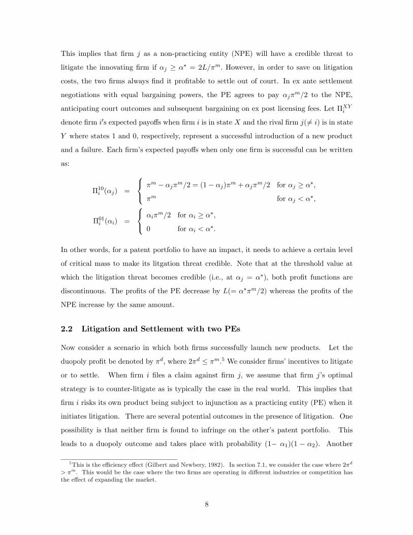
This implies that �rm j as a non-practicing entity (NPE) will have a credible threat to
litigate the innovating �rm if �j � �� = 2L=�m: However, in order to save on litigation
costs, the two �rms always �nd it pro�table to settle out of court. In ex ante settlement
negotiations with equal bargaining powers, the PE agrees to pay �j�m=2 to the NPE,
anticipating court outcomes and subsequent bargaining on ex post licensing fees. Let �XYi
denote �rm i0s expected payo¤s when �rm i is in state X and the rival �rm j(6= i) is in state
Y where states 1 and 0; respectively, represent a successful introduction of a new product
and a failure. Each �rm�s expected payo¤s when only one �rm is successful can be written
as:
�10i (�j) =
8<: �m � �j�m=2 = (1� �j)�m + �j�m=2 for �j � ��;
�m for �j < ��;
�01i (�i) =
8<: �i�m=2 for �i � ��;
0 for �i < ��:
In other words, for a patent portfolio to have an impact, it needs to achieve a certain level
of critical mass to make its litgation threat credible. Note that at the threshold value at
which the litigation threat becomes credible (i.e., at �j = ��), both pro�t functions are
discontinuous. The pro�ts of the PE decrease by L(= ���m=2) whereas the pro�ts of the
NPE increase by the same amount.
2.2 Litigation and Settlement with two PEs
Now consider a scenario in which both �rms successfully launch new products. Let the
duopoly pro�t be denoted by �d, where 2�d � �m:5 We consider �rms�incentives to litigate
or to settle. When �rm i �les a claim against �rm j; we assume that �rm j�s optimal
strategy is to counter-litigate as is typically the case in the real world. This implies that
�rm i risks its own product being subject to injunction as a practicing entity (PE) when it
initiates litigation. There are several potential outcomes in the presence of litigation. One
possibility is that neither �rm is found to infringe on the other�s patent portfolio. This
leads to a duopoly outcome and takes place with probability (1� �1)(1 � �2): Another
5This is the e¢ ciency e¤ect (Gilbert and Newbery, 1982). In section 7.1, we consider the case where 2�d
> �m: This would be the case where the two �rms are operating in di¤erent industries or competition hasthe e¤ect of expanding the market.
8
outcome that leads to a status quo is when both �rms are found to infringe on the other�s
patent portfolio. In such a case, we assume that they cross-license each other and maintain
a duopoly outcome. The remaining possibility is that one �rm, say �rm i, is found not
to infringe on �rm j�s while �rm j is found to infringe on �rm i�s patent portfolio. With
the assumption of 2�d � �m, there is no possibility of settlement and �rm i will be a
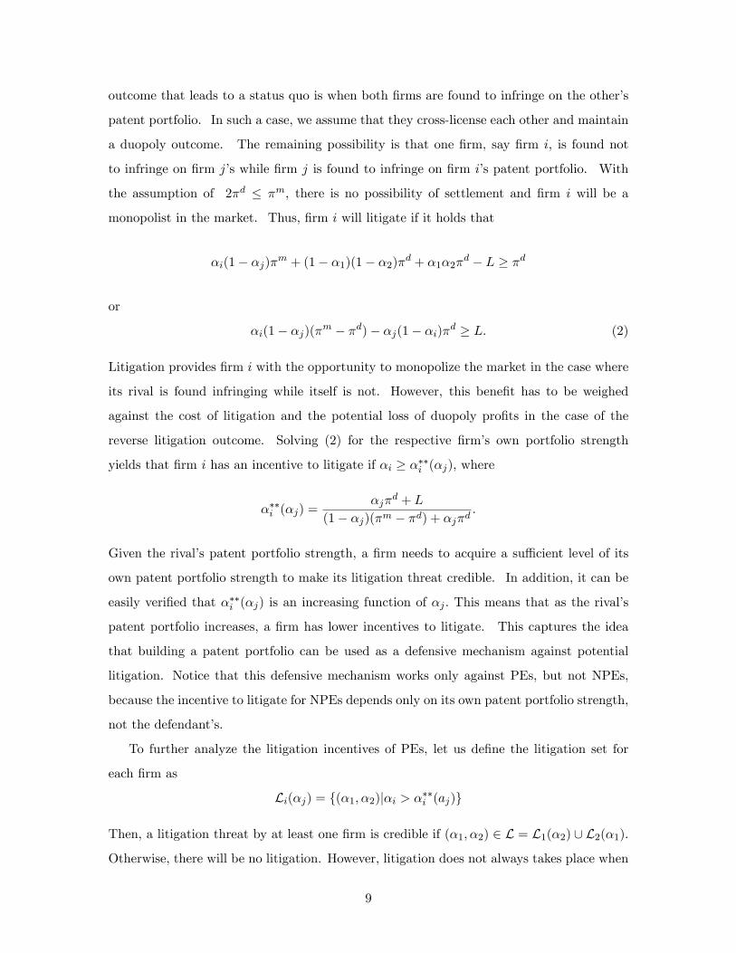
monopolist in the market. Thus, �rm i will litigate if it holds that
�i(1� �j)�m + (1� �1)(1� �2)�d + �1�2�d � L � �d
or
�i(1� �j)(�m � �d)� �j(1� �i)�d � L: (2)
Litigation provides �rm i with the opportunity to monopolize the market in the case where
its rival is found infringing while itself is not. However, this bene�t has to be weighed
against the cost of litigation and the potential loss of duopoly pro�ts in the case of the
reverse litigation outcome. Solving (2) for the respective �rm�s own portfolio strength
yields that �rm i has an incentive to litigate if �i � ���i (�j); where
���i (�j) =�j�
d + L
(1� �j)(�m � �d) + �j�d:
Given the rival�s patent portfolio strength, a �rm needs to acquire a su¢ cient level of its
own patent portfolio strength to make its litigation threat credible. In addition, it can be
easily veri�ed that ���i (�j) is an increasing function of �j : This means that as the rival�s
patent portfolio increases, a �rm has lower incentives to litigate. This captures the idea
that building a patent portfolio can be used as a defensive mechanism against potential
litigation. Notice that this defensive mechanism works only against PEs, but not NPEs,
because the incentive to litigate for NPEs depends only on its own patent portfolio strength,
not the defendant�s.
To further analyze the litigation incentives of PEs, let us de�ne the litigation set for
each �rm as
Li(�j) = f(�1; �2)j�i > ���i (aj)g
Then, a litigation threat by at least one �rm is credible if (�1; �2) 2 L = L1(�2) [ L2(�1):
Otherwise, there will be no litigation. However, litigation does not always takes place when
9
(�1; �2) 2 L. Firms can negotiate an out-of-court settlement to avoid the cost of litigation
before bringing an infringement suit. A settlement occurs and litigation is avoided if the
�rms�joint pro�ts from a duopoly outcome are higher than the joint expected pro�ts from
litigation, that is, if the following condition holds:
[�1(1� �2) + �2(1� �1)]�m + [1� (�1(1� �2) + �2(1� �1))]2�d � 2L < 2�d
or
(�1 + �2 � 2�1�2)(�m � 2�d) < 2L:
Let S be the set of (�1; �2) for which the above condition holds. Litigation takes place if
and only if (�1; �2) 2 eL = Lr S.By comparing the condition that de�nes each set, it can be easily veri�ed that when
both �rms have unilateral incentives to litigate, a settlement is not possible. To see this,
note that litigation occurs if the sum of LHS of condition (2) for both �rms is greater or
equal than the sum of the RHS of (2) for both �rms, that is, if
(�1 + �2 � 2�1�2)(�m � 2�d) � 2L: (3)
Let ���S (�2) denote the value of �1 such that this condition holds with equality. Condition
(3) is satis�ed when (2) holds and both �rms have an incentive to litigate. However, when
only one �rm, say only �rm i, has an incentive to litigate, i.e., (�1; �2) 2 (L r Lj(�i)); a
settlement is possible if (�1; �2) 2 S: This leads us to the following lemma.
Lemma 1 (L1(�2) \ L2(�1)) \ S = � and (L� Lj(�i)) \ S 6= �; where i = 1; 2; and j 6= i:
The lemma says that we can always �nd a set of parameters (�1; �2) where settlement takes
place when only one �rm has the incentive to litigate. However, litigation occurs despite
the possibility of out-of-court settlements if the expected gains in industry pro�t in the case
of asymmetric litigation outcomes outweigh the cost of litigation. This holds if either both
�rms unilaterally prefer litigation or if one �rm�s expected gains from litigation outweighs
the rival�s expected losses. Re�ecting the possibility of out-of-court settlements, we can
write each �rm�s expected pro�t when both �rms are PEs as follows:
10
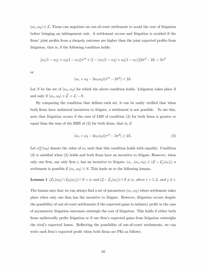
�11i (�i; �j) =
8>>><>>>:�i(1� �j)�m + (1� �1)(1� �2)�d + �1�2�d � L for (�1; �2) 2 eL�d + (�i � �j)�m=2 for (�1; �2) 2 L \ S
�d for (�1; �2) =2 L
The second case, (�1; �2) 2 L\S, occurs when exactly one �rm has an incentive to litigate
and industry pro�ts are maximized by settling out of court. Firms engage in Nash bargaining
and the �rm with the stronger patent portfolio, say �rm i (with �i > �j), receives (�i �
�j)�m=2 in settlement from its rival. The following proposition further characterizes the
equilibrium outcome of the litigation game with two PEs.
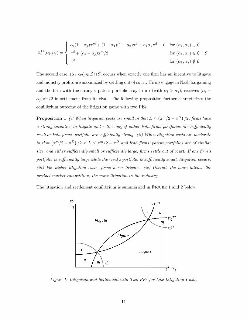
Proposition 1 (i) When litigation costs are small in that L ���m=2� �D
�=2, �rms have
a strong incentive to litigate and settle only if either both �rms portfolios are su¢ ciently
weak or both �rms�portfolio are su¢ ciently strong. (ii) When litigation costs are moderate
in that��m=2� �D
�=2 < L � �m=2 � �D and both �rms�patent portfolios are of similar
size, and either su¢ ciently small or su¢ ciently large, �rms settle out of court. If one �rm�s
portfolio is su¢ ciently large while the rival�s portfolio is su¢ ciently small, litigation occurs.
(iii) For higher litigation costs, �rms never litigate. (iv) Overall, the more intense the
product market competition, the more litigation in the industry.
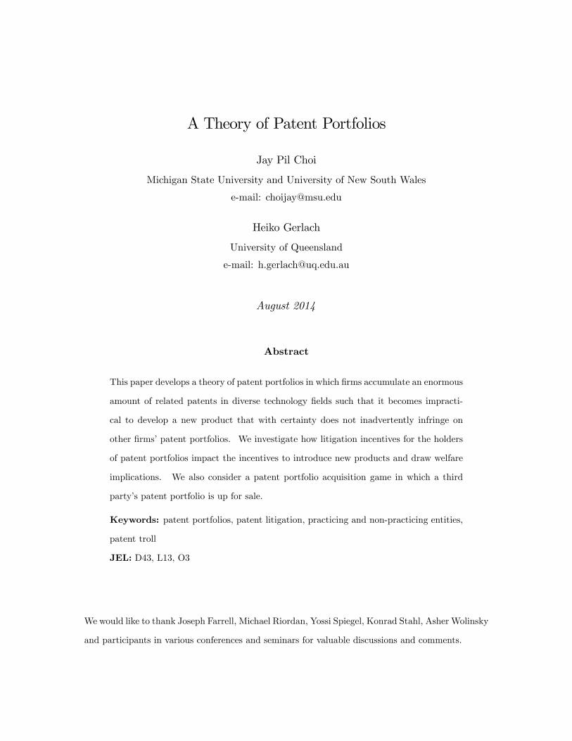
The litigation and settlement equilibrium is summarized in Figure 1 and 2 below.
Figure 1: Litigation and Settlement with Two PEs for Low Litigation Costs.
11
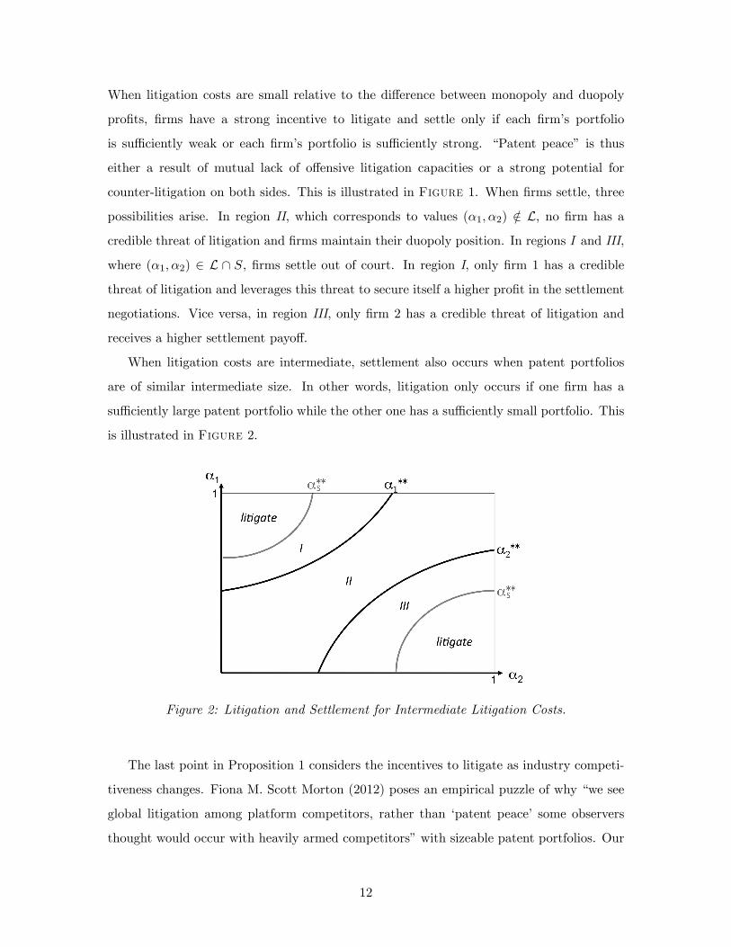
When litigation costs are small relative to the di¤erence between monopoly and duopoly
pro�ts, �rms have a strong incentive to litigate and settle only if each �rm�s portfolio
is su¢ ciently weak or each �rm�s portfolio is su¢ ciently strong. �Patent peace� is thus
either a result of mutual lack of o¤ensive litigation capacities or a strong potential for
counter-litigation on both sides. This is illustrated in Figure 1. When �rms settle, three
possibilities arise. In region II, which corresponds to values (�1; �2) =2 L, no �rm has a
credible threat of litigation and �rms maintain their duopoly position. In regions I and III,
where (�1; �2) 2 L \ S, �rms settle out of court. In region I, only �rm 1 has a credible
threat of litigation and leverages this threat to secure itself a higher pro�t in the settlement
negotiations. Vice versa, in region III, only �rm 2 has a credible threat of litigation and
receives a higher settlement payo¤.
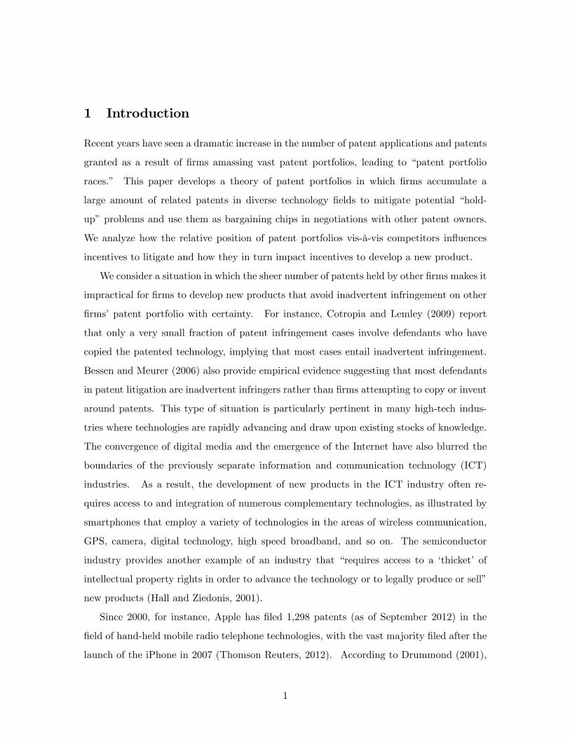
When litigation costs are intermediate, settlement also occurs when patent portfolios
are of similar intermediate size. In other words, litigation only occurs if one �rm has a
su¢ ciently large patent portfolio while the other one has a su¢ ciently small portfolio. This
is illustrated in Figure 2.
Figure 2: Litigation and Settlement for Intermediate Litigation Costs.
The last point in Proposition 1 considers the incentives to litigate as industry competi-
tiveness changes. Fiona M. Scott Morton (2012) poses an empirical puzzle of why �we see
global litigation among platform competitors, rather than �patent peace� some observers
thought would occur with heavily armed competitors�with sizeable patent portfolios. Our
12
model identi�es conditions under which such litigation takes place. In particular, as the
competitiveness of the industry intensi�es, the relative gains from excluding a rival through
litigation are higher (see condition (3)). Hence, we would expect to see more litigation
among PEs in industries where product market competition is more intense.6
2.3 Comparison of Litigation Incentives between NPE and PE
In recent years, serious concerns have been expressed regarding the role of NPEs in patent
litigation. Our analysis sheds some light on this. The above model partially con�rms
the conventional wisdom that NPEs have more incentives to litigate because they have
nothing to lose beyond the litigation costs whereas PEs risk their own products being
subjected to injunction when they initiate litigation. However, we can also show that there
is a countervailing mechanism that may induce PEs to have higher incentives to litigate
compared to NPEs. When NPEs litigate, the reward for a successful litigation is to share
the monopoly pro�t with the infringer. With Nash bargaining between the NPE and the
infringer, the payo¤ from successful litigation is �m=2: For PEs, the payo¤ from a successful
litigation outcome is the value of excluding its rival from the marketplace, (�m��d). In the
event of a negative litigation outcome, a PE is excluded from the marketplace and incurs
a loss of �d: Hence, the value of litigation is increasing in the intensity of product market
competition. Thus, when �d is small and competition is intense, we cannot rule out the
case where PEs have higher incentives to litigate compared to NPEs.
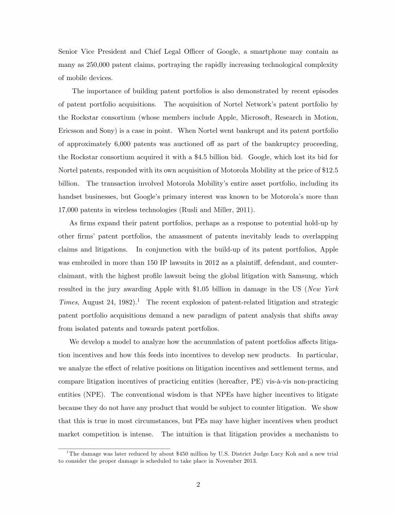
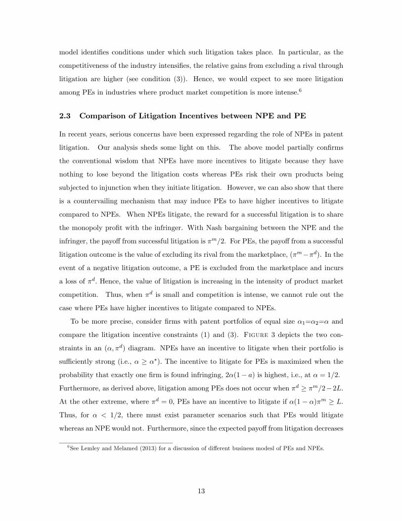
To be more precise, consider �rms with patent portfolios of equal size �1=�2=� and
compare the litigation incentive constraints (1) and (3). Figure 3 depicts the two con-
straints in an (�; �d) diagram. NPEs have an incentive to litigate when their portfolio is
su¢ ciently strong (i.e., � � ��): The incentive to litigate for PEs is maximized when the
probability that exactly one �rm is found infringing, 2�(1� a) is highest, i.e., at � = 1=2.
Furthermore, as derived above, litigation among PEs does not occur when �d � �m=2�2L:
At the other extreme, where �d = 0, PEs have an incentive to litigate if �(1 � �)�m � L.
Thus, for � < 1=2, there must exist parameter scenarios such that PEs would litigate
whereas an NPE would not. Furthermore, since the expected payo¤ from litigation decreases
6See Lemley and Melamed (2013) for a discussion of di¤erent business modesl of PEs and NPEs.
13
Figure 3: Litigation Incentives for PE versus NPE
in �d, there is a unique threshold value �d with
�d =�m
4
�m � 4L�m � 2L;
such that �d � �d is a necessary condition for PEs to have stronger litigation incentives.
We thus obtain the following result.
Lemma 2 If product market competition is intense and patent portfolios are neither too
small nor too big, then PEs have stronger incentives to litigate compared to NPEs. Other-
wise, NPEs have (weakly) more incentives to litigate.
3 Investment in New Product Development
One of the major concerns about the patent thicket and the accumulation of strategic
patent portfolios is their impact on innovative activities. In this section we analyze the
e¤ects of patent portfolios on the incentives to invest in R&D. For given patent portfolio
sizes (�1; �2), �rm i�s expected payo¤ when it invests Ii and the rival �rm invests Ij can be
written as
14
i(I1; I2;�1; �2) =p(Ii)p(Ij)�11i (�1; �2) + p(Ii)[1� p(Ij)]�10i (�j)
+ [1� p(Ii)]p(Ij)]�01i (�i)� Ii
Firm i�s optimal investment level, given Ij ; solves the following problem:
MaxIi
i(I1; I2;�1; �2):
The �rst order condition for optimal investment, @i=@Ii = 0, can be rewritten as
p(Ij)[�11i (�i; �j)��01i (�i)] + [1� p(Ij)]�10i (�j) =
1
p0(Ii): (4)
This equation implicitly de�nes �rm i�s reaction function Ii = Ri(Ij ;�1; �2). The LHS is
the expected bene�t of investing in a higher R&D success rate. The rival is successful with
probability p(Ij). In this case, a higher success rate for �rm i makes it more likely that both
�rms introduce new products and less likely that �rm i is an NPE facing a successful rival.
By contrast, when the rival is not successful, more investment leads to a higher probability
that �rm i is the only PE in the industry. Hence, higher pro�ts as a PE increase the
incentive to invest whereas higher pro�ts as an NPE, �01i (�i), lower R&D incentives.
The Nash equilibrium investment levels I�1 (�1; �2) and I�2 (�1; �2) are at the intersec-
tion of the �rms� reaction functions. We now conduct a comparative static analysis of
how changes in (�1; �2) a¤ect the equilibrium investment in product development (I�1 ; I�2 ):
Throughout this analysis we assume that the stability condition (see the appendix to the
next proposition) is satis�ed and we focus on situations where the unique Nash equilibium
is an interior solution. As a �rst step, compare the pro�t functions of PEs and NPEs.
Lemma 3 �10i (�j) � max[�11i (�1; �2);�01i (�i)]: The relative magnitudes of �
11i (�1; �2)
and �01i (�i), however, are ambiguous and depend on the competitiveness of the duopoly
outcome.
The lemma states that for any con�guration of patent portfolio positions, a �rm strictly
prefers to be the sole �rm that succeeds in product development. However, when the
other �rm is successful in the development of a new product, it is not necessarily better to
15
develop its own product and compete in the product market. It may be better to be an
NPE, especially when competition is intense and the other �rm has built a strong position
in its patent portfolio that can be used against the �rm in consideration. Lemma 3 directly
implies the following property.
Lemma 4 Investments in new product development are strategic substitutes.
We are now in a position to analyze the e¤ect of a unilateral increase in one �rm�s patent
portfolio position on investment.
Lemma 5 @Ri=@�j < 0, but the sign of @Ri=@�i is ambiguous. In particular, (i) if �rm
i has incentives to litigate only when it is a PE, @Ri=@�i > 0; (ii) if �rm i has incentives
to litigate only when it is an NPE, then @Ri=@�i < 0; and (iii) if �rm i has incentives to
litigate whenever �rm j develops a new product and �j < 1=2, then @Ri=@�i > 0:
Lemma 5 states that when �rm i�s patent portfolio size increases, the rival �rm j�s reaction
function in investment of new product development shifts inwards. However, the e¤ect on
its own product development is ambiguous. When �rm i�s litigation threat is credible for
�rm i whenever �rm j develops a new product, an increase in �rm i�s patent portfolio
induces its own reaction function to shift out only when �j < 1=2; that is, the rival �rm�s
patent portfolio size is not substantial.
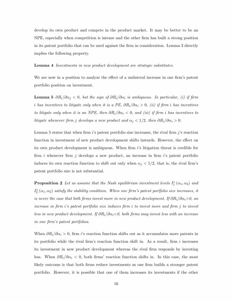
Proposition 2 Let us assume that the Nash equilibrium investment levels I�1 (�1; �2) and
I�2 (�1; �2) satisfy the stability condition. When one �rm�s patent portfolio size increases, it
is never the case that both �rms invest more in new product development. If @Ri=@�i>0, an
increase in �rm i�s patent portfolio size induces �rm i to invest more and �rm j to invest
less in new product development. If @Ri=@�i<0, both �rms may invest less with an increase
in one �rm�s patent portfolios.
When @Ri=@�i > 0; �rm i�s reaction function shifts out as it accumulates more patents in
its portfolio while the rival �rm�s reaction function shift in. As a result, �rm i increases
its investment in new product development whereas the rival �rm responds by investing
less. When @Ri=@�i < 0; both �rms� reaction function shifts in. In this case, the most
likely outcome is that both �rms reduce investments as one �rm builds a stronger patent
portfolio. However, it is possible that one of them increases its investments if the other
16
�rm�s reaction curve shifts relatively more. Yet, it is never possible that both �rms increase
their investment as a result of patent accumulation by one �rm.
4 Welfare e¤ects of strategic patent portfolios
Firms accumulate patent portfolios as a strategic response to potential litigation due to
inadvertent patent infringement. While it is impossible to prevent the formation of such
portfolios, we can consider their welfare e¤ects in conjunction with the underlying de�cien-
cies of the patent system. In other words, would consumer welfare increase in a world where
patents are ironclad and well-de�ned while �rms are perfectly informed and able to invent
around their rival�s patents?
In this section we address this issue by comparing two scenarios. The �rst scenario is
the set-up from the previous section. Patent validity and scope are uncertain and �rms
hold incomplete information about the patent positions of their rivals. In this case, patent
portfolios increase the risk of inadvertent infringement and ex post litigation. We dub this
the �patent uncertainty� scenario. In the second scenario, patents are ironclad and �rms
have ex ante complete information. That is, �rms are aware of all possible infringments
and are able to invent around their rival�s patents. This is the �complete information�or
�patent certainty�scenario. We compare ex ante consumer surplus in these two scenario.
First, we derive investment levels in the patent certainty scenario and compare with the
previous section. Then, we investigate overall ex ante expected consumer surplus.
Consider investment incentives in the patent certainty scenario. In the absence of inad-
vertent infringement and litigation, �rm i�s optimal investment, for a given rival investment
Ij , is
p(Ij)�d + [1� p(Ij)]�m =
1
p0(Ii): (5)
Compare this condition with the �rst-order condition (4) in the previous section. A su¢ cient
condition for both �rms to invest more with patent uncertainty is that each �rm�s respective
LHS in (4) is larger than the LHS of (5).7 The �rst term in each condition is the marginal
value of investing given the rival innovates. The value in (4), �11i (�i; �j) � �01i (�i), can
be larger than �d when the two innovating �rms litigate against each other in equilibrium,
7This is a su¢ cient condition when the �rms�patent portfolio positions are su¢ ciently similar in size.
17
that is for (�1; �2) 2 eL. The second term is the marginal investment value given the rival
is not active. In this case, the marginal value from investing is (at least weakly) larger in
the complete information scenario.
This implies that a necessary condition for �rms investing more with patent uncertainty
is that �rms litigate in the event that both introduce new products. For instance, consider
a situation in which NPEs do not have an incentive to litigate while PEs litigate.8 From
Lemma 2 it follows that such situations arise when product market competition is intense
and patent portfolios are neither too small nor too large. In those cases, we have �10i (�j) =
�m, �01i (�i) = 0 and, by (2), it holds that �11i (�i; �j) � �d: Hence, the LHS of (4) is strictly
larger than the LHS of (5) and both �rms invest strictly more under patent uncertainty.
Lemma 6 Suppose (�1; �2) 2 eL and ex post litigation arises when both �rms innovate.
There always exist parameter values such that �rms invest more with strategic patent port-
folios and patent uncertainty.
Litigation can increase industry pro�ts as it raises the probability of monopolistic market
outcomes. This implies that �rms may invest more in R&D when they hold patent portfolios
and there is the possibility of inadvertent infringement. In other words, strategic patent
portfolios might be able to restore one of the functions of the patent system itself, that is,
to encourage investment in new product development.
This result naturally raises the question as to how ex ante consumer surplus compares
in the two scenarios. To analyze this issue, let Sd and Sm denote consumer surplus in a
duopoly and monopoly outcome, respectively. Assume 0 � Sm � Sd. For simplicity, let us
focus on the case where patent portfolios unambiguously increase R&D investment. That is
the case for patent portfolio positions such that two innovating PEs litigate whereas NPEs
have no incentive to litigate. Furthermore, suppose that the �rms have patent portfolios
of the same size � and consider a symmetric equilibrium in investment. Let p denote the
common R&D success rate. The ex ante expected consumer surplus in the patent certainty
scenario is given by
CS0(p) = p2Sd + 2p(1� p)Sm
which is increasing in the success rate. Similarly, the ex ante expected consumer surplus
8 In the appendix to the next lemma we demonstrate that �rms might also invest more under patentuncertainty when NPEs do have an incentive to litigate.
18
with patent uncertainty and portfolio positions such that PEs litigate while NPE have no
incentive to litigate, is
CSp(p) = CS0(p)� p22�(1� �)(Sd � Sm):
At equal success rates, the consumer surplus is lower in the presence of patent uncertainty
due to the fact that when both �rms innovate and litigation ensues, there is a probability
that one �rm is able to exclude its rival from the marketplace. This is the static ine¢ ciency
of patent portfolios. By contrast, overall ex ante consumer surplus with patent uncertainty
is higher if
CS0(p(I�))� CS0(p(I0)) � p(I�)22�(1� �)(Sd � Sm); (6)
where I� and I0 denote the equilibrium investment levels under patent uncertainty and
patent certainty, respectively, with I� > I0. This condition holds if the increase in con-
sumer surplus due to more innovations outweighs the price e¤ect of exclusionary litigation
outcomes. Condition (6), for instance, is satis�ed in the following example.
Example 1 Consider a market for a homogenous good with a linear demand function
D(p)=1-p. When both �rms develop a new product, they compete in quantities. Suppose
�rms hold patent portfolios of equal size �. Further, �rms invest in R&D using p(I) =pI.
In this set-up, the equilibrium hazard rates are
p(I0) =�m
2 + �m � �d ; p(I�) =
�m
2 + �m ��11i (�; �):
Substituting these values and �m = 1=4; �d = 1=9; Sd = 2=9; Sm = 1=4 into (6) yields
2 + L
[77� �(1� a) + 36L]2� 2
772
which holds since (3) requires L � �(1� a)=36:
We thus derive the following result.
Proposition 3 In the presence of patent uncertainty, patent portfolios have two e¤ects on
consumer surplus. There is a negative, static e¤ect as litigation can reduce competition in
the marketplace. There is also a dynamic e¤ect as the prospect of litigation might increase
19
or decrease investment incentives. The latter e¤ect can dominate - and consumer surplus
can be higher under patent uncertainty - for patent portfolio positions such that litigation
arises when both �rms introduce new products.
5 Patent Portfolio Acquisition
Suppose that a patent portfolio of strength � > 0 has been put up for sale. The probability
that any new product infringes on some patents in the portfolio for sale is given by �:
Let us assume that the sale is via an ascending price auction. When this portfolio is
acquired, the acquiring �rm�s patent portfolio size and its strength increases. Let �+i be
the ex post patent portfolio strength when �rm i acquires the patent portfolio for sale. Let
�i(= �+
i ��i ) denote the incremental patent portfolio strength due to the acquisition where
�i is the strength of �rm i�s existing patent portfolio. Further, suppose that the infringing
probabilities on each patent portfolio are independent. Then, we have �i = (1��i)�, that
is,
�+
i = �i + (1� �i)�
Note that �i is decreasing in �i even though �+
i is increasing in �i: In other words, the
e¤ect of acquiring the additional patent portfolio on the strength of the existing patent
portfolio is decreasing in the original strength. For instance, if �i = 1; there would be no
impact on the strength of the patent portfolio, that is, �i = 0:
5.1 Patent Portfolio Acquisition Game between Two PEs
Consider two PEs with existing patent portfolios of size �1 and �2(� �1), respectively,
bidding for the available patent packet.9 Firm i�s willingness-to-pay is the di¤erence in
pro�ts from securing the patent portfolio itself and having its rival acquire it, that is,
�11i (�i + �i; �j)��11i (�i; �j + �j):
It is easy to verify that the �rm with the stronger existing patent portfolio, that is �rm 2,
has a higher willingness-to-pay for the patents if industry pro�ts are higher when �rm 2
9See Spulber (2013) for an interplay of innovation incentives and the possibility of intellectual property(IP) trade in a market for inventions.
20
buys relative to the case when �rm 1 buys, or
�11(�1; �2 + �2) � �11(�1 + �1; �2); (7)
where
�11(�1; �2) =2Xi=1
�11i (�1; �2):
The following lemma states that this condition always holds.
Lemma 7 The �rm with the larger patent portfolio has a (weakly) higher willingness-to-pay
for additional patents.
The �rm with the larger patent portfolio has a stronger incentive to accumulate more
patents. This is due to the fact that industry pro�ts are higher the more asymmetric
the patent portfolio distribution. Asymmetric patent portfolios increase the probability
that exactly one �rm can a¢ rm its patents in litigation and exclude its rival from the
marketplace. Lemma 7 thus implies that, in equilibrium, �rm 2�s bid is slightly higher than
the willingness-to-pay of �rm 1 and �rm 2 secures the patent packet. Hence, the di¤erence
in patent portfolio strength between the two �rms increases.
An interesting question is how the patent packet sale a¤ects consumer surplus. Let
CS11(�1; �2) denote expected consumer surplus when both �rms are PEs and hold patent
portfolios of strength �1 and �2; respectively. Consumers face a duopoly except for patent
portfolio constellations, in which �rms litigate and exactly one �rm is excluded. Hence, we
have
CS11(�1; �2) = Sd � [1� �1�2 � (1� �1)(1� �2)]
8<: Sd � Sm if (�1; �2) 2 eL;0 otherwise.
Now compare expected consumer surplus when �rm 1 and �rm 2 acquire the patent packet,
respectively. Suppose litigation always occurs independent of which �rm acquires the packet.
Then we get
CS11(�1 + �1; �2)� CS11(�1; �2 + �2) = 2�(�2 � �1)(Sd � Sm) > 0:
21
Furthermore, if there is litigation when �rm 2 acquires but not after �rm 1�s acquisition,
consumer surplus is always higher in the latter case. Thus, consumers are weakly better
o¤ when the �rm with the smaller portfolio acquires the patents. This leads to a more
even distribution of patents and a lower probability that one �rm is excluded from the
marketplace when litigation arises.
Proposition 4 In equilibrium the �rm with the larger patent portfolio acquires the addi-
tional patent packet while consumers would be better o¤ if the packet would be purchased by
the �rm with the weaker portfolio. The acquisition price (weakly) decreases in the degree of
product market competition between �rms.
This result might explain why Google lost in its bid for Nortel Network�s patent portfolio.
At the time of the patent auction, Google was in a very weak patent position compared
to its rivals. Apple, Microsoft and RIM had already amassed signi�cant patent portfolios.
Some commentators were thus surprised to see Google being outbid and foregoing the
opportunity to level the playing �eld. Our result suggests that intense product market
competition and the potential to exclude the rival through litigation made Nortel�s patent
packet more valuable to the Consortium members than to Google.
The acquisition price itself re�ects the pro�t di¤erence for �rm 1 between winning and
losing the auction. More intense competition reduces the acquisition price because the
probability of ending up in a duopoly after litigation has a positive cross derivative with
respect to �1 and �2. This implies that adding the packet for sale to the smaller portfolio
of �rm 1 increases the likelihood of a duopoly outcome more than adding it to the larger
portfolio of �rm 2. Hence, the higher duopoly pro�ts the larger the di¤erence between
winning and losing for �rm 1, and the larger the acquisition price.
5.2 Patent Portfolio Acquisition Game between PE and NPE
By contrast, consider a patent portfolio acquisition game between one PE and one NPE.
Without any loss of generality, let �rm 1 be PE and �rm 2 be NPE. As is clear from the
pro�t de�nitions in Section 2, the PE�s portfolio strength does not �gure into the �rms�
payo¤ functions. The only reason for the PE to acquire the available patent packet is to
prevent an NPE from using it in settlement negotiations or in litigation against the PE.
Since PE and NPE always settle on license terms in equilibrium rather than litigate their
22
disputes to completion, it is clear that the willingness-to-pay for the patent portfolio is the
same for both �rms, that is,
�101 (�2)��101 (�2 + �2) = �012 (�2 + �2)��012 (�2)
=
8>>><>>>:0 if �2 + �2 < ��
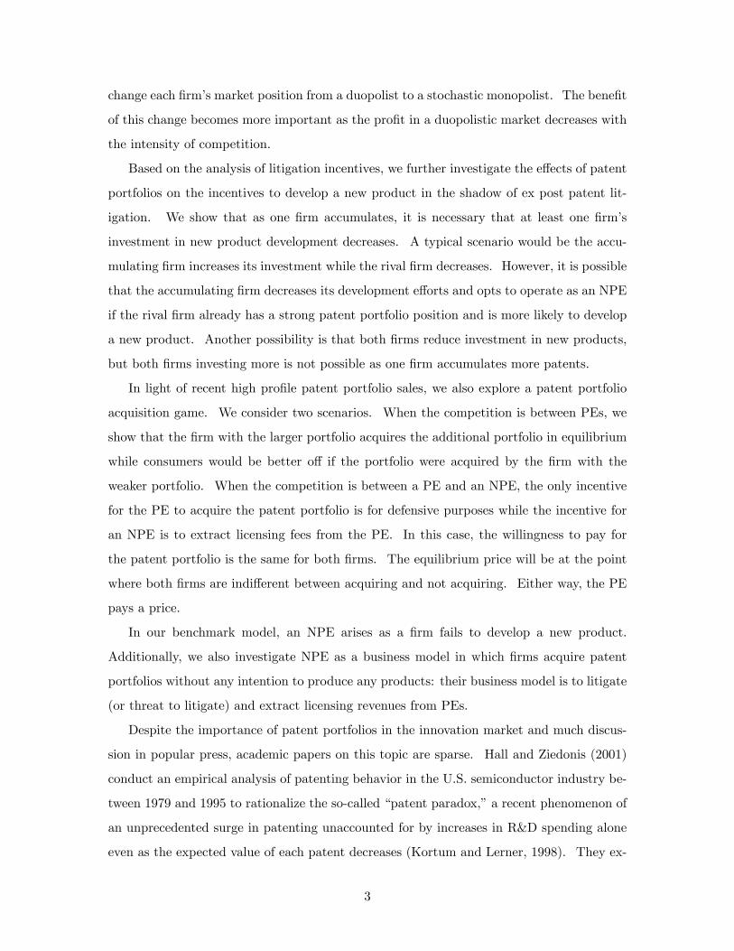
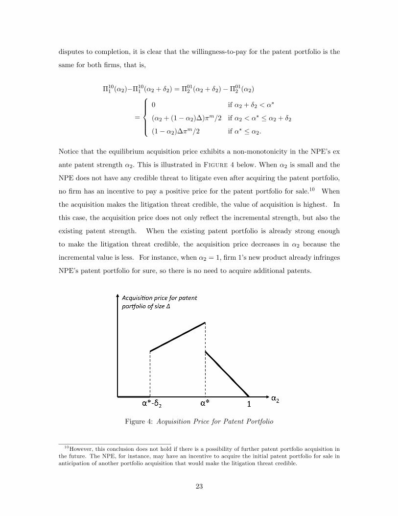
(�2 + (1� �2)�)�m=2 if �2 < �� � �2 + �2(1� �2)��m=2 if �� � �2:
Notice that the equilibrium acquisition price exhibits a non-monotonicity in the NPE�s ex
ante patent strength �2: This is illustrated in Figure 4 below. When �2 is small and the
NPE does not have any credible threat to litigate even after acquiring the patent portfolio,
no �rm has an incentive to pay a positive price for the patent portfolio for sale.10 When
the acquisition makes the litigation threat credible, the value of acquisition is highest. In
this case, the acquisition price does not only re�ect the incremental strength, but also the
existing patent strength. When the existing patent portfolio is already strong enough
to make the litigation threat credible, the acquisition price decreases in �2 because the
incremental value is less. For instance, when �2 = 1; �rm 1�s new product already infringes
NPE�s patent portfolio for sure, so there is no need to acquire additional patents.
Figure 4: Acquisition Price for Patent Portfolio
10However, this conclusion does not hold if there is a possibility of further patent portfolio acquisition inthe future. The NPE, for instance, may have an incentive to acquire the initial patent portfolio for sale inanticipation of another portfolio acquisition that would make the litigation threat credible.
23
6 NPE as a Business Model
The analysis so far has assumed that all �rms have the ability to manufacture and market
new products. A �rm becomes an NPE when its investment fails to produce a new product.
However, in recent years the number of companies whose business model is purely based
on converting intellectual property into licensing revenues (�patent trolls�) has sharply
increased. In this section, we analyze NPEs as a business model to accommodate this
possibility. Section 5 analyzes a patent portfolio acquisition game at the litigation stage
after the outcomes of new product development. In this section, we analyze the incentive to
acquire a patent portfolio for sale in anticipation of new product development. To simplify
the analysis, we consider a case where �rm 1 is potentially a PE, but �rm 2 is an NPE
without any manufacturing capacity whose main source of revenues is through licensing.
When �rm 2 is an NPE that does not engage in any new product development, the only
thing that matters is the strength of �rm 2�s patent portfolio because �rm 1 cannot litigate
against �rm 2. We have to consider three cases.
Case 1: �2 � ��. In this case, �rm 2 has incentives to litigate even if it does not acquire
a new patent portfolio for sale when �rm 1 has a new product. Let us de�ne
'(�2) =MaxI1
p(I1)�101 (�2)� I1:
Let I�1 (�2) denote the maximizer of this objective. Note that I�1 (�2) is decreasing in �2;
and @'(�2)=@�2 = � p(I�1 (�2))�m=2 < 0 by the envelope theorem: Firm 1�s incentive to
acquire the additional patent packet is purely for defensive purposes to prevent the NPE
from acquiring it. Firm 1�s maximum willingness to pay to acquire the patents for sale is
given by
B1 = '(�2)� '(�2 + �2) = �Z �2+�2
�2
@'(x)
@xdx =
�m
2
Z �2+�2
�2
p(I�1 (x))dx
The incentives for �rm 2 to acquire the additional patents come from the exclusionary value,
and �rm 2�s maximum willingness to pay is given by
B2 = [p(I�1 (�2 + �2))(�2 + �2)� p(I�1 (�2))�2]
�m
2:
24
Case 2: �2 < �� < �+2 : In this case, �rm 2 does not have a credible threat to litigate against
�rm 1 without acquiring the patent portfolio for sale, but its threat becomes credible after
acquisition. In other words,
�101 (�2) = �m; �101 (�
+2 ) = (1�
�+22)�m
In this case, the PE�s willingness to pay for the patent packet for sale is
B1 = '(�2)� '(�2 + �2)
= [p(I�1 (�2))�m � I�1 (�2)]� [p(I�1 (�+2 ))(1�
�+22)�m � p(I�1 (�+2 ))]
whereas the NPE�s maximum willingness to pay is given by
B2 = p(I�1 (�
+2 ))
�+22�m:
Case 3: �+2 < ��: Here, the patent portfolio for sale has no value to the PE and NPE.
Comparing the willingness-to-pay B1 and B2 in all cases, we obtain the following outcome
of the patent sale.
Proposition 5 If the patent sale occurs before the development of the new product, then
the PE has a (weakly) higher willingness-to-pay and acquires the patent portfolio.
The intuition for this result is that the NPE can extract rents only when the PE develops
a new product. The acquisition of additional portfolio is bene�cial ex post, but adversely
a¤ects the PE�s investment incentives. This adverse impact on the PE�s investment incen-
tives discourages the NPE�s patent portfolio acquisition. This e¤ect is absent when the
acquisition auction takes place after the development of the new product.
Our analysis also reveals the incentives for NPEs to acquire a patent portfolio in secret.
This is in sharp contrast to PEs� practice. Chien (2010) makes a distinction between
contrasting strategies of �patent signal�and �patent secrecy�. When �rms acquire a patent
portfolio to deter litigation by other PEs, they publicize their patent portfolio to send
a message to competitors: �If sued, I have the ability to retaliate.�11 However, the so-
called patent trolls exploit secrecy. Intellectual Ventures, Acadia, and many others have
11Chien (2010), p. 319.
25
assigned their patents to thousands of shell companies and subsidiaries, making them hard
to track. For instance, Ewing and Feldman (2011) identi�ed 1276 shell companies created
by Intellectual Ventures. It is their explicit strategy to wait until PEs develop products
that infringe on their patent portfolios to �surprise them with a suit.�
7 Extensions and Robustness
In this section, we extend our analysis into two directions and check the robustness of our
main results.
7.1 The Market Expansion E¤ect
So far we have assumed that the two �rms are competing in the same market. With the
assumption of 2�d � �m; this implies that there is no licensing between PEs when one �rm
is found to infringe upon the other�s patent portfolio, but the latter does not infringe upon
the former�s. We now consider the possibility of market expansion with licensing between
PEs. To formalize this, suppose that each �rm�s new product covers a market size of 1.
However, there is an overlap between the two �rms�customer base of size (1� s). In other
words, for the market size of s, each �rm is a monopolist, but for the remaining area of
(1� s) they compete. Thus, the parameter s represents the market expansion e¤ect when
both PEs produce compared to only one PE producing.12 When s = 1; their markets do
not overlap and the market expansion e¤ect is the largest. Our previous analysis is the
special case of s = 0:
When one �rm is a PE and the other is NPE, market expansion is not possible and the
previous analysis applies. Now let us consider the case of two PEs. If they do not engage
in litigation, their individual payo¤s are given by s�m+ (1 � s)�d. When �rm i litigates
against �rm j; again, it is �rm j�s best interest to counter-litigate. With the probability of
(1� �1)(1 � �2); neither �rm is found to infringe on the other�s patent portfolio. In this
case, the pre-litigation situation persists with each �rm earning s�m+ (1� s)�d: Another
outcome that leads to a status quo is when both �rms are found to infringe on the other�s
patent portfolio. The remaining possibility is that one �rm, say �rm i, is found not to
12To be more precise, the parameter s captures two e¤ects, a market size expansion and a relative increasein the monopolistic versus the competitive market segment. Since both e¤ects individually yield the samequalitative results in our framework, we have subsumed them into one parameter.
26
infringe on �rm j�s while �rm j is found to infringe on �rm i�s patent portfolio. In this
case, �rm i can license its patent portfolio and enable �rm j to enter its markets.13 A
license agreement is feasible if licensing increases industry pro�ts relative to the situation
where �rm i supplies the competitive market segment as well as its exclusive segment as
a monopolist. This holds if the gain from supplying �rm j exclusive market segment via
licensing outweighs the introduction of duopolistic competition in the contested market
segment,
s�m � (1� s)(�m � 2�d) or s � �m=2� �d�m � �d � sL:
Licensing occurs when the market expansion e¤ect is su¢ ciently large and product market
competition in the contested segment is weak. What are the e¤ects of licensing and the
market expansion e¤ect on litigation incentives? First, suppose s is su¢ ciently large such
that licensing occurs if exactly one �rm can assert its patent portfolio in litigation. Licensing
then yields an industry pro�t of 2s�m+(1�s)�d, which is exactly the industry pro�t when
�rms refrain from litigation. Since litigation is costly, it will never occur if �rms have ex
post incentives to license. By contrast, if s is su¢ ciently small, licensing does not arise
ex post. In this case litigation is optimal for �rms if the industry pro�ts from asymmetric
litigation outcomes and monopolization of the contested market segment exceed the status
quo industry pro�ts for symmetric outcomes and the cost of litigation, that is,
[�1(1� �2) + �2(1� �1)]�m � 2L � [1� �1(1� �2)� �2(1� �1)]h2s�m + (1� s)�d
ior
s � sL �L
[1� �1(1� �2)� �2(1� �1)] (�m � �d):
Thus, three parameter regions exist. For high values of s and low product market competi-
tion, there is no litigation and no licensing. For intermediate values of the market expansion
e¤ect, �rms have no incentive to license ex post but litigation is too costly. Finally, if the
market expansion e¤ect is not too strong and product market competition in the contested
segment is intense, �rms litigate and refrain from licensing when exactly one �rm asserts
its property rights during litigation.
13Alternatively, �rm i could license its patents for use in �rm j�s monopolistic market segment only. Thiswould not a¤ect the qualitative nature of our results.
27
Proposition 6 When product market competition is less intense, the market expansion
e¤ect may induce �rms to license ex post rather than to litigate.
7.2 Asymmetric Product Market Positions
In our above analysis we allow �rms to hold patent portfolios of di¤erent sizes but assume
that they have symmetric positions in product market competition. In this extension, we
investigate the e¤ect of product market position on litigation incentives for given symmetric
patent portfolios of size �1=�2=�. Which �rm has a stronger incentive to litigate, the
market leader or the �rm with the smaller market share? What is the impact of �rm
asymmetry on litigation in equilibrium? To address these questions in a simple way, assume
that �rms di¤er in their marginal cost of production. In particular, let ci denote the marginal
cost of production of �rm i such that c1 = c � � and consider c2 = c + � where � � 0 is
our measure for cost asymmetry. Further let �m(c) denote the monopoly pro�t with cost c
and �d(ci; �) the duopoly pro�t of �rm i. The parameter � � 0 represents the intensity of
competition in the market. For � = 0 the �rms�products are independent and as � goes to
in�nity, products become perfect substitutes. We impose the following two assumptions:14
A.1@��d(c1; �)� �d(c2; �)
�@�
� 0
A.2@��d(c1; �) + �
d(c2; �)�
@�� 0;
@2��d(c1; �) + �
d(c2; �)�
@�@�� 0:
The �rst condition states that the pro�t advantage of the low-cost �rm increases as products
become closer substitutes. The second set of assumptions implies that cost asymmetry
increases industry duopoly pro�ts and that this e¤ect is stronger when products are closer
substitutes.
First, consider �rms�unilateral incentives to litigate. Firm i has an incentive to litigate
if
L � �(1� �)h�m(ci)� 2�d(ci)
i:
Comparing the individual litigation constraints yields that the �rm with the higher marginal
14These assumptions are satis�ed for the most commonly used demand structures such as the ones inSingh and Vives (1984) or Shubik and Levitan (1980).
28
cost (�rm 2) has a stronger incentive to litigate if and only if
�m(c2)� 2�d(c2) � �m(c1)� 2�d(c1): (8)
This condition always hold under assumption A.1 as the smaller �rm stands to gain more
from excluding its rival. Similarly, �rms prefer litigation over settlement if
�(1� �)h�m(c� �) + �m(c+ �)� 2�d(c� �)� 2�d(c+ �)
i� 2L: (9)
Monopoly pro�ts are decreasing and convex in cost. Hence, the sum of monopoly pro�ts in
the squared bracket increases in the degree of cost asymmetry. However, under assumption
A.2 cost asymmetries increase duopoly industry pro�ts more and the LHS is decreasing in
the parameter �. It follows that in industries with asymmetric product market positions,
�rms litigate less in equilibrium.
Proposition 7 The �rm with the smaller market share has a stronger incentive to litigate.
Asymmetric product market positions reduce overall litigation incentives in the industry.
8 Concluding Remarks
The patent system is created as a mechanism to encourage discovery and development
of new ideas and technologies. However, the current patent system has been criticized
and described to be under siege due to an explosion of suspect quality, overlapping, and
excessively broad patents. With the convergence of technologies in various high-tech �elds, it
is inevitable for new products to incorporate complementary technologies and inadvertently
infringe on patented technologies developed elsewhere. This has led to patent portfolio races
in which �rms competitively build up an ever increasing size of patent portfolios by internal
R&D and/or acquisition of patents held by other �rms. In this paper, we have developed
a model to analyze the implications of such patent portfolios on the incentives to develop
new products in the shadow of patent litigation.
We showed that the incentives to litigate for practicing entities depend crucially on the
competitiveness of the industry. The e¤ects of an increase in one �rm�s patent portfolios
unambiguously reduce the rival �rm�s incentives to develop a new product. However, an
increase in its own patent portfolio does not necessarily induce more incentives to develop
29
its own new product. In such a case, the patent build-up by one �rm can unambiguously
reduce the overall rate of new product developments.
Our analysis can be extended to address many other unexplored issues. For instance,
we have assumed that the extent of patent portfolios held by each �rm is common knowl-
edge. However, there are many examples in which companies with new products and
services have been held up by patent asserting entities unknownst to them. Our model
can help identify circumstances under which �rms with a large patent portfolio would have
incentives to exploit secrecy to their advantage. One way to achieve secrecy is to create
shell companies and subsidiaries, which makes it di¢ cult to track the ownership of patents.
For instance, Intellectual Ventures has created more than 1200 shell companies (Ewing and
Feldman, 2012). The secrecy allows patent-assertion entities to use a surprise tactic by
litigating (unknowingly) infringing �rms at the most vulnerable time when they have sunk
their resources in designing new products (Shapiro, 2010) while maintaining other �rms�in-
centives to introduce new products by keeping them in the dark. Finally, we have analyzed
the e¤ects of given sizes of patent portfolios on new product developments. It would be
interesting to analyze the strategic incentives to build up patent portfolios and the optimal
composition of patent portfolios in more detail.
Appendix
Proof of Lemma 1 and Proposition 1. From (3) it follows that �rms litigate if and
only if
�1(1� 2�2)(�m � 2�d) � 2L� �2(�m � 2�d):
For �2 < 1=2; �rms settle if
�1 �2L� �2(�m � 2�d)(1� 2�2)(�m � 2�d)
� ���S (�2):
When �2 is su¢ ciently small, this threshold value is strictly positive and continuous in �2.
Thus, �rms settle if both portfolios are su¢ ciently small. For �2 > 1=2; �rms settle if
�1 � ���S (�2):
30
It holds that
���S (�2 = 1) =�m � 2�d � 2L�m � 2�d < 1:
As ���(�2) is continuous, there must exist values such that �rms settle if both portfolios
are su¢ ciently strong. This proves the �rst point in Proposition 1. Further note that
���S (�2 = 0) =2L
�m � 2�d < 1
if and only if
�m=2� �d � L: (10)
Hence, there exist values (�1; �2) such that �rms litigate if �rm 1�s portfolio is su¢ ciently
strong while �rm 2�s portfolio is su¢ ciently weak. Similarly, condition (10) implies that
���S (�2 = 1) � 0:
Thus, �rms litigate if �rm 1�s portfolio is su¢ ciently weak and �rm 2�s portfolio is su¢ ciently
strong. This proves the second statement. In order to further characterize the settlement
and litigation behavior, check that
@���S@�2
= ��m
2 � �D � 2L(1� 2�2)2(�
m
2 � �D)
which implies
sign(@���S@�2
) =
8>>><>>>:�1 if �
m
2 � �D > 2L;
0 if �m
2 � �D = 2L;
1 if �m
2 � �D < 2L:
���������Further check that
@���1@�2
=L(�m � 2�d) + �d(�m � �d)[(1� �2)(�m � �d) + �2�d]2
> 0;
@2���1(@�2)2
=2(�m � 2�d)
�L(�m � 2�d) + �d(�m � �d)
�[(1� �2)(�m � �d) + �2�d]3
> 0
Similarly, let ���2 (�2) denote the value of �1 such that (2) holds with equality for �rm i=2,
���2 (�2) =�2(�
m � �d)� L�2(�m � 2�d) + �d
31
and
@���2 (�2)
@�2=
L(�m � 2�d) + �d(�m � �d)[�2(�m � 2�d) + �d]2
> 0;
@2���2 (�2)
(@�2)2= �
2(�m � 2�d)�L(�m � 2�d) + �d(�m � �d)
�[�2(�m � 2�d) + �d]3
< 0:
Finally note that ���1 (�2) � ���2 (�2) if and only if
�2(1� �2)(�m
2� �D) � L
2
This condition holds for any �2 if
�m
2� �D < 2L:
The qualitative properties of the graphs in Figure 1 and 2 in the main text and the
proposition follow. �
Proof of Lemma 3. �10i (�j) is a decreasing function of �j with the minimum value of�m
2
when �j = 1 whereas �01i (�i) is an increasing function of �i with the maximum value of
�m=2 when �1 = 1: Thus, �10i (�j) � �01i (�i) for all (�1; �2) with the equality holding only
at �1=�2=1: Note that �11i (�1; �2) increases in �d: It achieves the highest value when �d =
�m=2; in which case its value is given by (1+�i��j)�m=2; which is less than (2��j)�m=2(=
�10i (�j)): Taken together, this implies that �10i (�j) � max[�11i (�1; �2);�
01i (�i)]: How-
ever, the relative magnitudes of �11i (�1; �2) and �01i (�i) are ambiguous. For instance,
�11i (�1; �2) > �01i (�i) if �
d = �m=2, whereas �01i (�i) > �11i (�1; �2) if �
d = 0 and �j > 1=2:
Since �11i (�1; �2) is an increasing in �d and decreasing in �j while �01i (�i) is independent
of �d and �j ; �11i (�1; �2) is more likely to be larger than �01i (�i) for a higher �
d and a
lower �j : �
Proof of Lemma 4. By totally di¤erentiating the �rst order condition (4) with respect
to I1 and I2; we derive
R0i(Ij ;�1; �2) =
dIidIj
= �p0(Ii)p0(Ij)[�11i (�i; �j)��10i (�j)��01i (�i)]
[SOCi]< 0;
where [SOCi] = p00(Ii)[p(Ij)�11i (�i; �j) + (1 � p(Ij))�10i (�j) � p(Ij)�01i (�i)] < 0: The in-
32
equality follows from Lemma 3. �
Proof of Lemma 5. By totally di¤erentiating the �rst order condition (4) with respect
to Ii and �j ; we have
@Ri@�j
= � p0(Ii)
[SOCi][p(Ij)
@�11i (�i; �j)
@�j+ (1� p(Ij))
�10i (�j)
@�j] � 0
since @�11i (�i; �j)=@�j � 0 and @�10i (�j)=@�j � 0: Similarly, a total di¤erentiation of (4)
with respect to Ii and �i yields
@Ri@�i
= �p0(Ii)p(Ij)
[SOCi][@�11i (�i; �j)
@�i� �
01i (�i)
@�i]:
Thus, the sign of @Ri=@�i equals the sign of [@�11i (�i; �j)=@�i � @�01i (�i)=@�i]; which is
ambiguous since
@�11i (�i; �j)
@�i=
8>>><>>>:(1� �j)(�m � �d) + �j�d for (�1; �2) 2 eL�m=2 for (�1; �2) 2 L \ S
0 for (�1; �2) =2 L
and
@�01i (�i)
@�i=
8<: �m=2 for �i � ��;
0 for �i < ��:
In situations where PEs have an incentive to litigate whereas NPEs do not, the sign is
de�nitely positive. Vice versa, when PEs have no incentive to litigate whereas NPEs would,
the sign is negative. When PEs litigate and NPE have an incentive to litigate, we get
@�11i (�i; �j)
@�i� @�
01i (�i)
@�i= (
1
2� �j)(�m � 2�d)
which is positive if and only if �j < 1=2: �
Proof of Proposition 2. Let us totally di¤erentiate the �rst order conditions for I1 and
I2 with respect to �1:
@21@I21
dI1 +@21@I1@I2
dI2 +@21@I1@�1
d�1 = 0
@22@I1@I2
dI1 +@22@I22
dI2 +@22@I2@�1
d�1 = 0
33
To derive comparative statics result with respect to �1, we can write the expression above
in the following matrix form.
24 @21@I21
@21@I1@I2
@22@I1@I2
@22@I22
3524 dI1d�1
dI2d�1
35 =24 � @21
@I1@�1
� @22@I2@�1
35By applying Cramer�s rule, we can derive
dI1d�1
=
24 � @21@I1@�1
@21@I1@I2
� @22@I2@�1
@22@I22
35jAj =
� @21@I1@�1
@22@I22
+ @22@I2@�1
@21@I1@I2
jAj
dI2d�1
=
24 @21@I21
� @21@I1@�1
@22@I1@I2
� @22@I2@�1
35jAj =
�@21@I21
@22@I2@�1
+ @22@I1@I2
@21@I1@�1
jAj
where jAj =
������@21@I21
@21@I1@I2
@22@I1@I2
@22@I22
������ > 0 by the stability condition. Thus,
sign[dI1d�1
] = sign[� @21@I1@�1
@22@I22
+@22@I2@�1
@21@I1@I2
]
sign[dI2d�1
] = sign[�@21@I21
@22@I2@�1
+@22@I1@I2
@21@I1@�1
]
We know that @21@I21
< 0 and @22@I22
< 0 by the second order condition. In addition,
sign[ @22
@I2@�1] = sign[@R2@�1
] < 0 by Lemma 5. We thus have:
(i)When @R1@�1
> 0; the result is unambiguous in that dI1d�1
> 0 and dI2d�1
< 0:
(ii)When @R1@�1
< 0; the signs of dI1d�1
and dI2d�1
are ambiguous. However, both cannot be
positive. We prove this by contradiction. Suppose that dI1d�1
> 0 and dI2d�1
> 0: For this to
happen, it must be that
���� @21@I1@I2
���� >������@21@I1@�1
@22@I22
@22@I2@�1
������ and���� @22@I1@I2
���� >������@21@I21
@22@I2@�1
@21@I1@�1
������This implies that ���� @21@I1@I2
@22@I1@I2
���� > ���� @21@I1@�1
@21@I21
����34
However, the condition above contradicts our stability condition. �
Proof of Lemma 6. The second case arises when PEs litigate and NPEs have an
incentive to litigate after at least one innovation is introduced. Firms invest more under
patent uncertainty if
p(Ij)[�11i (�i; �j)� �d + �m ��01i (�i)��10i (�j)] > �m ��10i (�j):
For simplicity, consider the symmetric case when both �rms hold patent portfolios of the
same size �. With litigation incentives in place, it holds that �m = �01i (�) + �10i (�) and
we can rewrite the condition as
p(Ij) >��m=2
�(1� �)(�m � 2�d)� L:
If the rival�s investment is su¢ ciently high, the �rm�s reaction function shifts outwards.
Hence, if the equilibrium investment with complete information is less than this threshold
value, equilibrium investment with patent uncertainty is higher. �
Proof of Lemma 7. First check the condition for the case when litigation occurs no
matter who buys the patent portfolio,
�11(�1; �2 + �2)j(�1;�2+�2)2 eL ��11(�1 + �1; �2)j(�1+�1;�2)2 eL (11)
= �(�2 � �1)(�m � 2�d) � 0
Next check the case where litigation arises if �rm 2 obtains the patent portfolio but not
when �rm 1 acquires it. This holds when
�11(�1; �2 + �2)j(�1;�2+�2)2 eL � 2�d > �11(�1 + �1; �2 +�)j(�1+�1;�2)2 eL:In this case, �11(�1 + �1; �2) = 2�d and condition (7) always holds. From (11) it follows
that it is never possible that after �rm 1�s acquisition, there is litigation while there is no
litigation after �rm 2�s acquisition. Finally, if there is no litigation after acquisition by any
of the two �rms, the industry pro�ts equal 2�d and condition (7) is satis�ed with equality.
The lemma follows. �
Proof of Proposition 5. We show B1 > B2: First, consider Case 1. Since I�1 (�2) is
35
decreasing in �2; we have
B1 =�m
2
Z �2+�2
�2
p(I�1 (x))dx >�m
2p(I�1 (�2 + �2))�2:
Note that
�2p(I�1 (�2 + �2)) > p(I
�1 (�2 + �2))�2 � [p(I�1 (�2))� p(I�1 (�2 + �2))]�2
= p(I�1 (�2 + �2))(�2 + �2)� p(I�1 (�2))�2
Therefore, B1 > B2: For Case 2 we have
B1 �B2 = [p(I�1 (�2))�m � I�1 (�2)]� [p(I�1 (�+2 ))�m � I�1 (�+2 )] > 0
by a revealed preference argument. �
Proof of Proposition 6. First, check that condition (8) is always satis�ed for �=0
since �d(ci; �=0) = �m(ci): By assumption A.1, this condition becomes less restrictive as �
increases and the result follows. Second, take the derivative of the LHS of (9) with respect
to �
@�m(c+ �)
@�� @�
m(c� �)@�
+ 2@�d(c� �; � = 0)
@�� 2@�
d(c+ �; � = 0)
@�
=@�m(c+ �)
@�� @�
m(c� �)@�
+ 2@�m(c� �)
@�� 2@�
m(c+ �)
@�
=@�m(c� �)
@�� @�
m(c+ �)
@�< 0:
Furthermore, by assumption A.2 the derivative of the LHS decreases further as � increases
and the result follows. �
References
[1] Bessen, James and Meurer, Michael J., �Patent Litigation with Endogenous Disputes,�
American Economic Review, 96, no. 2, 2006, pp. 77-81.
[2] Bessen, James and Meurer, Michael J., �The Direct Costs from NPE Disputes,�Cornell
Law Review, forthcoming.
36
[3] Chien, Colleen V., "From Arms Race to Marketplace: The Complex Patent Ecosystem
and Its Implications for the Patent System," Hastings Law Journal, December 2010,
pp. 297-355.
[4] Chiou, Jing-Yuan, "The Dilemma of Defensive Patenting," unpublished manuscript,
January 2013.
[5] Cotripia, Christopher Anthony and Lemley, Mark A., "Copying in Patent Law," North
Carolina Law Review, 2009, pp. 1421-1466.
[6] Denicolo, Vincenzo and Zanchettin, Piercarlo, "A Dynamic Model of Patent Portfolio
Races," Economics Letters, 2012, pp. 924-927.
[7] Drummond, David, "When Patents Attack Android," August 3, 2001, available at
http://googleblog.blogspot.com/2011/08/when-patents-attack-android.html.
[8] Ewing, Tom and Feldman, Robin, "The Giants Among Us," Standford Technology Law
Review, 2012.
[9] Gallini, Nancy, "Deterrence by Market Sharing: A Strategic Incentive for Licensing,"
American Economic Review, 1984, pp. 931-941.
[10] Gilbert, Richard and Newbery, David, "Preemptive Patenting and the Persistence of
Monopoly," American Economic Review, 1982, pp. 514-526.
[11] Hagiu, Andrei and Yo¢ e, David B., "The New Patent Intermediaries: Platforms, De-
fensive Aggregators, and Super-Aggregators," Journal of Economic Perspectives, 2013,
pp. 45-66.
[12] Hall, Bronwyn H. and Ziedonis, Rosemarie Ham, "The Patent Paradox Revisited: An
Empirical Study of Patenting in the U.S. Semiconductor Industry, 1979-1995," Rand
Journal of Economics, 2001, pp. 101-128.
[13] Kortum, Samuel and Lerner, Josh, "Stronger Protection or Technological Revolution"
What is Behind the Recent Surge in Patening?" Carnegie-Rochester Conference Series
on Pulbic Policy, 1998, pp. 247-304.
[14] Lemley, Mark A. and Melamed, Douglas, "Missing the Forest for the Trolls," Columbia
Law Review, 2013, pp. 2117-2189.
37
[15] Mazzeo, Michael J., Hillel, Jonathan, and Zyontz, Samantha, "Do NPEs Matter?:
Non-Practicing Entities and Patent Litigation Outcomes," unpublished manuscript,
2013.
[16] Morton, Fiona M. Scott, "Patent Portfolio Acquisitions: An Economic
Analysis," presented at Fifth Annual Searle Conference on Antitrust
Economics and Competition Policy, September 21, 2012, available at
http://www.justice.gov/atr/public/speeches/288072.pdf.
[17] Morton, Fiona Scott and Shapiro, Carl, "Strategic Patent Acquisitions," 2013, available
at http://papers.ssrn.com/sol3/papers.cfm?abstract_id=2288911.
[18] Parchomovsky, Gideon and Wagner, R. Polk, "Patent Portfolios," University of Penn-
sylvania Law Review, 2005, Vol. 154, No.1., pp. 1-77.
[19] Rusli, Evelyn M. and Miller Calire Cain, "Google to Buy Motorola Mo-
bility for $12.5 Billion," New York Times, August 15, 2011, available at
http://dealbook.nytimes.com/2011/08/15/google-to-buy-motorola-mobility/
[20] Shapiro, C., "Prior User Rights," American Economic Review, May 2006, pp. 92-96.
[21] Shapiro, C., "Injunctions, Hold-Up, and Patent Royalties," American Law and Eco-
nomics Review, 2010, pp. 1-39.
[22] Shubik, Martin and Richard Levitan, "Market Structure and Behavior," Cambridge,
Massachusetts: Havard University Press.
[23] Siebert, Ralph and von Graevenitz, Georg, "Jostling for Advantage or Not: Choosing
between Patent Portfolio Races and Ex Ante Licensing," Journal of Economic Behavior
and Organizatioin, 2010, pp. 225-245.
[24] Singh, Nirvikar and Xavier Vives, "Price and quantity competition in a di¤erentiated
duopoly," Rand Journal of Economics 15(4), 1984, pp. 546-554.
[25] Spulber, Daniel F., "How Do Competitive Pressures A¤ect Incentives to Innovate When
There Is a Market for Inventions?," Journal of Political Economy, 2013, pp. 1007-1054.
[26] Thomson Reuters, "Inside the iPhone Patent Portfolio," September 2012.
38
[27] Ziedonis, Rosemarie Ham, "Don�t Fence Me In: Fragmented Markets for Technology
and the Patent Acquisition Strategies of Firms," Management Science, 2004, pp. 804-
820.
39
Recommended