DYNAMIC BEHAVIOUR OF
LVL-CONCRETE COMPOSITE
FLOORING SYSTEMS
Ph.D Thesis
Nor Hayati Abd. Ghafar
2015
Supervisors
Prof. Andy Buchanan
Assoc. Prof. Massimo Fragiacomo
Dr Zainah Ibrahim

Special dedication to
my late mum, your love always with us
‘FARIDAH SALLEH’
(1959-2010)
i
Abstract
An LVL-concrete composite floor (LCC) is a hybrid flooring system, which
was adapted from a timber-concrete composite (TCC) floor system. By replacing the
timber or glulam joists with LVL joists, the strength of the floor was increased.
However, the demand nowadays is to build longer spans and this may reduce the
stiffness and lead to the floor being more susceptible to vibration problems.
While the vibration problem may not be as critical as other structural issues,
people could feel sick and not comfortable if the floor vibrates at the resonant
frequency of the human body. Hence, this research focuses on the dynamic behaviour
of long span LCC flooring systems. Experimental testing and finite element modelling
was used to determine the dynamic behaviour, with particular regard to the natural
frequency, fn and mode shape of an LCC floor.
Initially, a representative series of LVL-concrete composite specimen types
were built starting from (1) full-scale T-joist specimens, (2) reduced-scale (one-third)
multi-span T-joist specimens and (3) reduced-scale (one-third) 3m x 3 m floor. The
specimens were tested using an electrodynamic shaker. The SAP 2000 finite element
modelling package was used to model and evaluate the full- and reduced-scale LVL-
concrete composite T-joist experimental results. Additionally, a 8m x 7.8 m LCC floor
was modelled and analysed using SAP 2000. The behaviour of the 8m LCC floor was
investigated through the changing of (1) concrete topping thickness, (2) depth of LVL
joist, (3) different types of boundary conditions, and (4) the stiffness of the connectors.
Both the experimental results and the finite element analyses agreed and
showed that increased stiffness increased the natural frequency of the floor, and the
boundary conditions influenced the dynamic behaviour of the LCC floor. Providing
more restraint increased the stiffness of the floor system. The connectors' stiffness did
not influence the dynamic performance of the floor.
The study outcomes were based on a 8 Hz natural frequency limitation where
the fundamental natural frequency of the LCC floor must exceed 8 Hz in order to
prevent vibration problems. The research showed that a 8 m LCC long span floor can
be constructed using LVL joists of between 300 mm to 400 mm depth with a concrete
thickness of 65 mm for the longer spans, and joists of between 150 mm to 240 mm
depth in conjunction with a concrete topping thickness of 100 mm for the shorter spans.

ii
Acknowledgments
First and foremost to the great Allah Almighty, for giving me the strength to
face all the obstacles and challenges, including two major earthquakes for me to
complete this research successfully.
I would like to thank University Tun Hussein Onn Malaysia and the Ministry
of High Education, Malaysia for giving me a big opportunity to further my study and
for providing the scholarship.
The big thanks are to my supervisors, Prof. Andy Buchanan, Assoc. Prof
Massimo Fragiacomo and Dr Zainah Ibrahim who never stopped giving me their
knowledge for all the time of the research. Also to Dr. Bruce Deam and Assoc.
Professor Peter Moss for your help and encouragement, insight and advice that have
been invaluable to the success of this work. Also to Dr. David Carradine for your
kindness helping me in the laboratory and being a part of this project.
Thanks are also expressed to David Yeoh, Marta Martalli and Kyle Chaning-
Pearch who were directly involved during the experimental phase in this project. Also
thanks to John Maley, Tim Perigo, Gavin Keats, Nigel Dixon and other UC technicians
who were directly and indirectly involved. Special thanks to Vinod Sadashiva and
Charlotte Brown for their kindness.
In a addition, I would like to thank my family specially for dad, Asyikin
(adik), Ain, Azli and Saaidah (Ucu), my best friends ever (Hartini, Mariyam, Farah
Dina and Nastaein), and my flatmates (Fatanah, Shazlina and Ummu) for their support
and putting up with me during the ups and downs of the last four years.
Finally, very deep appreciation to my husband, Wan Afnizan for always being
there to support, encourage and be patient throughout the course of this work for the
last few years.
iii
TABLE OF CONTENTS
ABSTRACT..... ......................................................................................................................... I
ACKNOWLEDGMENTS ...................................................................................................... II
TABLE OF CONTENTS ..................................................................................................... III
LIST OF FIGURES .............................................................................................................. VI
LIST OF TABLES ............................................................................................................. VIII
LIST OF SYMBOLS ............................................................................................................ IX
CHAPTER 1 INTRODUCTION.......................................................................................... 1
1.1 Aims and Objectives of the Research 2
1.2 Scope of the Research 2
1.3 Methodology of the Research 4
1.4 Significance of the study 4
1.5 Outline of Thesis 5
CHAPTER 2 LITERATURE REVIEW ............................................................................. 8
2.1 Timber-concrete composite (TCC) floor system 8
2.1.1 Development of TCC 11
2.1.2 Design of TCC floors 14
2.1.3 LVL-Concrete Composite Flooring System 15
2.2 Floor Vibration 18
2.2.1 Floor Vibration Assessment 19
2.2.2 Vibration Assessment on Timber-Concrete Composite (TCC) Floor 21
2.2.3 Human Perception of Floor Vibration 22
2.2.4 Design Criteria for Floor Vibration 24
2.2.5 Use of Dampers to Control Floor Vibrations 37
2.3 Summary 37
CHAPTER 3 FULL-SCALE LCC T-JOIST SPECIMENS ............................................ 39
3.1 LCC T-joist Specimen Details 40
3.2 Experiment Modal Testing Method 44
iv
3.3 Modal Parameter Extraction Method 46
3.4 Dynamic performance of LCC T-joist specimens 49
3.5 Effect of span length 54
3.6 Effect of topping width 54
3.7 Effect of support stiffness 55
3.8 Finite Element Modelling of LCC T-joist specimens 58
3.9 Comparison between the modal test (EMA) and finite element modelling (FEA)
63
3.10 Damping from Impact Hammer Test 65
3.11 Conclusion and Summary 68
CHAPTER 4 EXPERIMENTAL MODAL ANALYSIS (EMA) ON REDUCED
SCALE LVL-CONCRETE COMPOSITE (LCC) T-JOIST
SPECIMENS ................................................................................................ 70
4.1 Construction Detail of Reduced Scale specimens 71
4.1.1 Multi-span specimen detail 71
4.1.2 Multi-storey specimen detail 73
4.1.3 Single-bay T-joist floor details 75
4.2 Dynamic performance of multi-span specimens 76
4.3 Dynamic performance of multi-storey specimens 78
4.4 Dynamic performance of a single-bay floor 80
4.5 Conclusion and Summary 82
CHAPTER 5 ANALYTICAL MODELLING OF REDUCED SCALE LCC T-JOIST
SPECIMENSAND FLOORS ...................................................................... 84
5.1 Multi-span specimens 88
5.2 Multi-storey specimens 96
5.3 Single-bay T-joist floor 100
5.4 Discussion 101
5.5 Summary and Conclusions 105
CHAPTER 6 ANALYTICAL MODELLING OF FULL-SCALE T-JOIST LCC
FLOOR ....................................................................................................... 107
6.1 8 m x 7.8 m T-joist LCC floor model 107
6.2 8 m x 7.8 m T-joist LCC floor behaviour 110
6.3 Effect of connector stiffness 116
6.4 Effect of concrete topping thickness 117
6.5 Effect of LVL joist depth 118
6.6 Relationship between concrete topping thickness and LVL joist depth 120
6.7 Conclusion and Summary 125
v
CHAPTER 7 DESIGN FOR VIBRATION OF LVL- CONCRETE COMPOSITE
(LCC) FLOORS ........................................................................................ 126
7.1 Introduction 126
7.2 Design criteria 127
7.3 Preliminary design 127
7.4 Advanced design method 128
7.5 Simple design method 132
7.6 Worked Example 134
7.7 Summary 137
CHAPTER 8 CONCLUSIONS AND RECOMMENDATIONS FOR FURTHER
WORK ........................................................................................................ 138
8.1 Research objectives 138
8.2 Research Summary 138
8.3 Recommendations for designers 140
8.4 Recommendation for Further Research 141
REFERENCES ..................................................................................................................... 142
APPENDIX A MATERIAL PROPERTIES ..................................................................... 147
APPENDIX B WORKED EXAMPLE .............................................................................. 148
vi
LIST OF FIGURES
Figure 2-1 Timber-concrete interlayer connections ............................................................................. 13
Figure 2-2 Proposed semi-prefabricated TCC floor system (Yeoh, 2008) ............................................. 17
Figure 2-3 Layout details of semi-prefabricated ‘M’ panel (a) off-site panel, ..................................... 17
Figure 2-4 A person perform the heel drop test and the time history of the test ............................... 20
Figure 2-5 Evaluation of human sensitivity by acceleration or velocity response versus natural
frequency, fn ........................................................................................................................ 23
Figure 2-6 Reiher-Meister scale ............................................................................................................ 25
Figure 2-7 Modified Reiher-Meister scale ............................................................................................ 26
Figure 2-8 Recommended peak acceleration for human comfort for vibration due to human activity
(source : Murray et al.,2003) ................................................................................................................ 28
Figure 2-9 Relationship between a and b (CEN, 2008b) ....................................................................... 31
Figure 3-1 (a) LVL-concrete composite specimen detail and ................................................................ 41
Figure 3-2 (a) 8 m LVL-concrete composite specimen with single LVL and .......................................... 41
Figure 3-3 (a) 8 m LVL-concrete composite specimen with double LVL and ....................................... 42
Figure 3-4 (a) 10 m LVL-concrete composite specimen and ................................................................. 42
Figure 3-5 Layout of 6 m beam ............................................................................................................. 43
Figure 3-6 Different types of support condition ................................................................................... 43
Figure 3-7 Location of exciter and node points along the LVL joist ...................................................... 44
Figure 3-8 Response of Specimen A ...................................................................................................... 48
Figure 3-9 Theoretical mode shape for simply supported beam.......................................................... 51
Figure 3-10 The first three mode shape of 6 m and 8 m specimens from vibration tests ................... 51
Figure 3-11 End support condition before and after being fixed to the ground .................................. 53
Figure 3-12 (a) Boundary stiffness a timber block as support and (b) mesh model ............................. 57
Figure 3-13 Finite element model ......................................................................................................... 57
Figure 3-14 Support effective width ..................................................................................................... 58
Figure 3-15 Lumped mass system ......................................................................................................... 59
Figure 3-16 LCC finite element models ................................................................................................. 60
Figure 3-17 Connection experimental load-slip curve (source: Yeoh (2010)) ...................................... 60
Figure 3-18 Mode shapes from finite element modelling for 6 m and 8 m specimens........................ 62
Figure 3-19 Comparison of 6 m specimens with and without cantilever arm ...................................... 62
Figure 3-20 A person striking the specimen and the time history of the impact force ....................... 65
Figure 3-21 Beam responses from impact hammer test ...................................................................... 66
Figure 3-22 Decay of motion ................................................................................................................ 67
Figure 3-23 Critical damping ratio ........................................................................................................ 67
Figure 3-24 Natural frequency limitation for a LCC flooring system .................................................... 69
Figure 4-1 Photographs of the multi-span system ................................................................................ 72
Figure 4-2 Concrete topping being cut to split the beams .................................................................. 73
Figure 4-3 Multi-storey single-bay systems .......................................................................................... 74
Figure 4-4 2-storey, 2-bay T-joist beams ............................................................................................. 74
Figure 4-5 Floor plan layout (dimension in mm) .................................................................................. 75
Figure 4-6 Cross-section A - A .............................................................................................................. 75
Figure 4-7 Multi-span mode shape ....................................................................................................... 78
vii
Figure 4-8 Multi-storey mode shape .................................................................................................... 80
Figure 4-9 Vibration test layout for single-bay floor ............................................................................. 81
Figure 4-10 Mode shape for single-bay floor ........................................................................................ 81
Figure 4-11 Mode shapes curve to the perpendicular of the joist span ............................................... 82
Figure 5-1 FE modelling elements representing structure components .............................................. 84
Figure 5-2 FE model for continuous T-joist specimen .......................................................................... 85
Figure 5-3 Details of timber block, joist and joist hanger (unit in mm) ................................................ 86
Figure 5-4 Natural frequency and mode shape for 1-span specimen .................................................. 90
Figure 5-5 Natural frequency and mode shape for 2-span specimen .................................................. 91
Figure 5-6 Natural frequency and mode shape for 3-span specimen .................................................. 92
Figure 5-7 Natural frequency and mode shape for 3-span specimen (cont') ....................................... 93
Figure 5-8 Natural frequency and mode shape for 4-span specimen .................................................. 94
Figure 5-9 Natural frequency and mode shape for 4-span specimen (cont') ....................................... 95
Figure 5-10 Natural frequencies and mode shapes for a 2-storey specimen ....................................... 96
Figure 5-11 Natural frequencies and mode shapes for a 3-storey specimen ....................................... 97
Figure 5-12 Natural frequencies and mode shapes for a 4-storey specimen ....................................... 98
Figure 5-13 Mode shape behaviour for a 2-bay, 2-storey specimen .................................................... 99
Figure 5-14 Natural frequencies and mode shapes for a single-bay 3 m x 3 m floor ......................... 100
Figure 5-15 Comparative mode shapes for multi-span LCC specimens .............................................. 103
Figure 5-16 Comparative mode shapes for multi-storey LCC specimens ........................................... 104
Figure 5-17 Comparative mode shapes for the single-bay LCC floor ................................................. 105
Figure 6-1 FE model of a floor strip of 8 m x 0.6 ................................................................................ 108
Figure 6-2 The model of an 8 m x 7.8 m T-joist LCC floor .................................................................. 108
Figure 6-3 Natural frequency vs number of nodes for mesh size of the floor strip ........................... 109
Figure 6-4 Different types of support system ..................................................................................... 111
Figure 6-5 Natural frequency of different types of support systems ................................................. 113
Figure 6-6 Mode shapes of LCC floor with different types of support system .................................. 114
Figure 6-7 Comparison of natural frequency for different types of connector stiffness ................... 117
Figure 6-8 The first six modes of vibration with increasing concrete topping thickness ................... 118
Figure 6-9 The first six modes of vibration with increasing depth of LVL joist ................................... 119
Figure 6-10 Comparison of natural frequencies for different concrete topping thickness ................ 122
Figure 6-11 Comparison of natural frequencies for different LVL joist depths .................................. 123
viii
LIST OF TABLES
Table 2-1 Advantages of TCC Floor System........................................................................................... 10
Table 2-2 Recommended Values of Parameters, Po, , and ao/g limit ................................................. 27
Table 2-3 Recommended Acceleration Limits for Vibrations Due to Rhythmic Activities (Murray et.al,
2003) ...................................................................................................................................... 28
Table 2-4 Summary of design methods to control vibrations in timber floors .................................... 35
Table 2-5 Acceptance criteria over time (Murray et.al, 2003).............................................................. 36
Table 3-1 Detail of LCC T-joist specimens ............................................................................................. 40
Table 3-2 Main digital data acquisition parameters adopted for FRF measurements ......................... 47
Table 3-3 Results of vibration tests on LCC simply supported specimens ........................................... 49
Table 3-4 Comparison of modal properties between a single and a sweep sinusoidal vibration test on
8 m specimen ........................................................................................................................ 52
Table 3-5 Comparison of modal properties between a non-fixed and a fixed support ....................... 53
Table 3-6 Comparison of modal properties between different span lengths ...................................... 54
Table 3-7 Comparison of modal properties between different topping widths .................................. 55
Table 3-8 Comparison of natural frequencies between different support conditions ......................... 56
Table 3-9 Summary of results from the finite element modelling ....................................................... 61
Table 3-10 Comparison between FEA and EMA for different support stiffnesses ............................... 64
Table 4-1 Results of vibration test on LCC multi-span specimens ........................................................ 76
Table 4-2 Result summary of multi-storey specimens .......................................................................... 79
Table 5-1 Stiffness properties of the springs ........................................................................................ 86
Table 5-2 Prediction of natural frequency for multi-span specimens .................................................. 88
Table 5-3 Comparison of fundamental natural frequency, f1 ............................................................. 101
Table 5-4 Comparison of the natural frequencies of a single-bay LCC floor ...................................... 101
Table 6-1 Limitation of concrete topping thickness for 8 m x 7.8 m LCC floor .................................. 121
Table 6-2 Percentage difference between SAP model and Eurocode 5 formula .............................. 124
Table 7-1 Suggested topping thickness for LCC floors based on 8 Hz limitation ................................ 128
ix
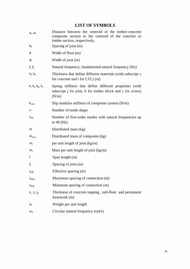
LIST OF SYMBOLS
ac, at Distance between the centroid of the timber-concrete
composite section to the centroid of the concrete or
timber section, respectively.
b1 Spacing of joist (m)
d Width of floor (m)
dt Width of joist (m)
f, fn Natural frequency, fundamental natural frequency (Hz)
hc, ht Thickness that define different materials (with subscript c
for concrete and t for LVL) (m)
k, kj, kb, kc Spring stiffness that define different properties (with
subscript j for joist, b for timber block and c for screw)
(N/m)
kcom Slip modulus stiffness of composite system (N/m)
n Number of mode shape
n40 Number of first-order modes with natural frequencies up
to 40 (Hz)
m Distributed mass (kg)
mcom Distributed mass of composite (kg)
mJ per unit length of joist (kg/m)
mt Mass per unit length of joist (kg/m)
l Span length (m)
lt Spacing of joist (m)
seff Effective spacing (m)
smax Maximum spacing of connection (m)
smin Minimum spacing of connection (m)
tc, ts, tp Thickness of concrete topping , sub-floor and permanent
formwork (m)
w Weight per unit length
wn Circular natural frequency (rad/s)
x
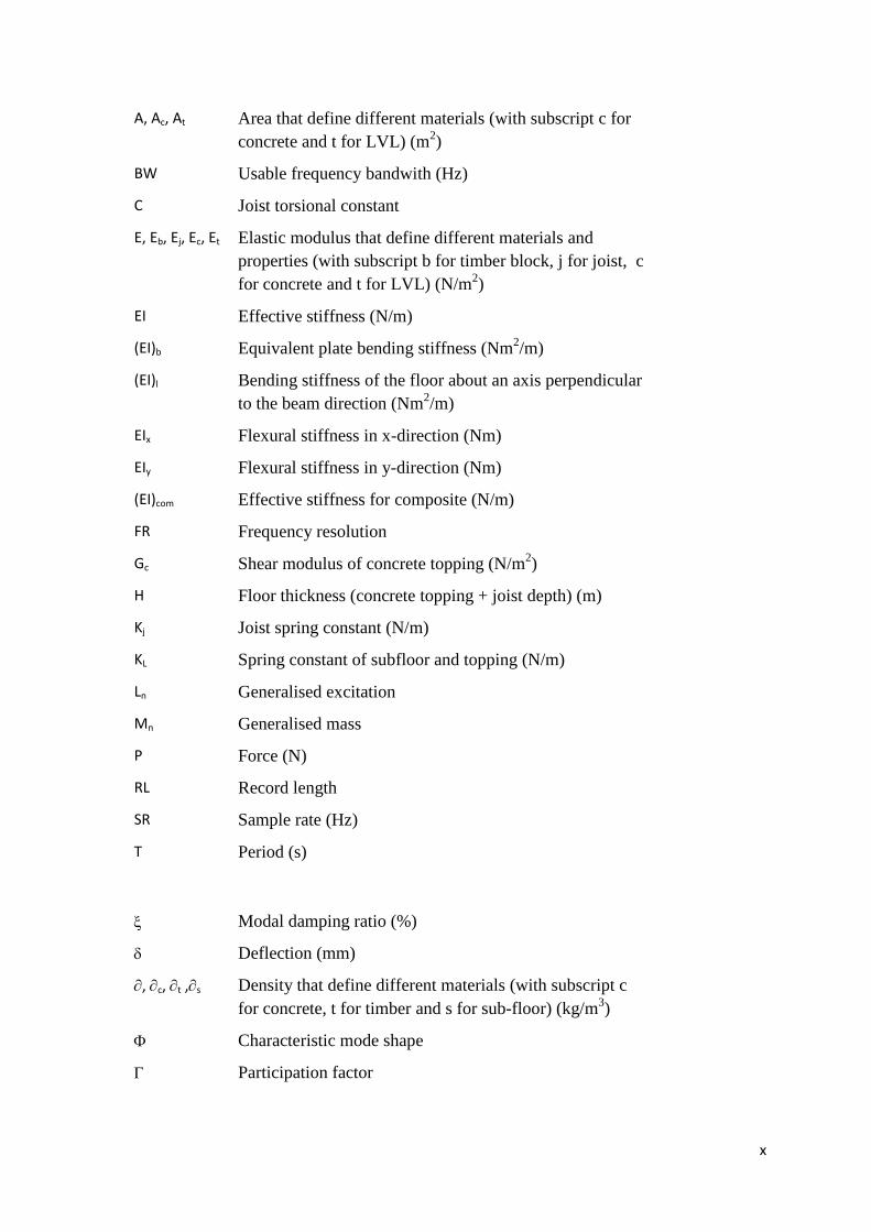
A, Ac, At Area that define different materials (with subscript c for
concrete and t for LVL) (m2)
BW Usable frequency bandwith (Hz)
C Joist torsional constant
E, Eb, Ej, Ec, Et Elastic modulus that define different materials and
properties (with subscript b for timber block, j for joist, c
for concrete and t for LVL) (N/m2)
EI Effective stiffness (N/m)
(EI)b Equivalent plate bending stiffness (Nm2/m)
(EI)l Bending stiffness of the floor about an axis perpendicular
to the beam direction (Nm2/m)
EIx Flexural stiffness in x-direction (Nm)
EIy Flexural stiffness in y-direction (Nm)
(EI)com Effective stiffness for composite (N/m)
FR Frequency resolution
Gc Shear modulus of concrete topping (N/m2)
H Floor thickness (concrete topping + joist depth) (m)
Kj Joist spring constant (N/m)
KL Spring constant of subfloor and topping (N/m)
Ln Generalised excitation
Mn Generalised mass
P Force (N)
RL Record length
SR Sample rate (Hz)
T Period (s)
Modal damping ratio (%)
Deflection (mm)
, c, t ,s Density that define different materials (with subscript c
for concrete, t for timber and s for sub-floor) (kg/m3)
Characteristic mode shape
Participation factor

xi
EMA Experimental Modal Analysis
FEA Finite Element Analysis
LCC LVL Concrete Composite
LVL Laminated Veneer Lumber
TCC Timber Concrete Composite
CHAPTER 1 INTRODUCTION
This thesis considers the dynamic performance of LVL-concrete composite
(LCC) floor systems. LCC floor systems are hybrid structures in which solid timber or
glued laminated timber beams are connected to a concrete slab in order to develop
composite action. The new application of laminated veneer lumber (LVL) instead of
sawn timber or glued laminated timber can further improve the performance of the
timber-concrete composite (TCC) system. TCC and LCC are nearly the same, but LVL
has higher strength and reduced variability, as a more reliable engineering material.
The composite action has to resist slip forces between timber and concrete.
According to Ceccotti (1995), the TCC structure is distinguished by a bending stiffness
much higher than the simple timber beam or concrete slab on their own. In comparison
with reinforced concrete floors, the TCC floors are lighter and more sustainable. In
comparison with timber floors, they are characterised by greater strength and stiffness,
increased thermal mass, better acoustic separation and they are less susceptible to
vibration.
These systems are an innovative system of timber structures to meet the
demand for high-performance long-span floors. However, there is still a concern about
serviceability vibration in the case of medium to long span LCC floors. These
serviceability vibration problems can occur due to human activities like walking,
running and jumping, which provide a repetitive loading on the floor. When the load
variation has the same frequency as the natural frequency of the floor, resonance can
occur and make other users feel uncomfortable and annoyed.
As retrofitting the floor to eliminate resonance can be quite expensive and
difficult, the best way is to design the floor properly at the start by having an adequate
understanding of the physical phenomena and a regard for the consequences of poor
design. Thus, a LCC floor system has been constructed and tested at the University of
Canterbury in collaboration with Carter Holt Harvey Wood products, a local New
Zealand manufacturer of LVL. The performance of dynamic behaviour, natural
2
frequency and mode shape of the LCC floor was investigated. The study was continued
by carrying out finite element modelling using SAP 2000 software to verify the
experimental work as well as to explore the influences of concrete topping thickness,
LVL joist depth, boundary conditions and connection stiffness. A simple design method
proposed for predicting the response of the LCC floor, for a complicated flooring
system is discussed at the end of this research.
1.1 Aims and Objectives of the Research
The main objective for this research is to provide a better understanding of the
vibration performance of LCC floors. The investigation is focussed on the dynamic
behaviour of LCC floors, including natural frequencies, damping ratio and mode
behaviours, and also the effect of boundary conditions.
In order to improve the knowledge of the dynamic behaviour of LVL-concrete
composite T-joist floors and to provide some recommendations to control the vibration
of these floors, the following specific research objectives were developed:
1. Experimentally characterise the dynamic performance (specifically the natural
frequencies, equivalent viscous damping ratios and mode shapes) of full- and
reduced-scale LVL-concrete composite floor system beams and floors.
2. Implement numerical finite element modelling of the tested structures, full- and
reduced-scale beams and floors, using the results from experimental modal
analysis to verify the models.
3. Propose a simple design method for control of vibration at the serviceability limit
state based on finite element modelling results.
1.2 Scope of the Research
The scope of the investigation of the dynamic behaviour of LCC T-joist
specimens and floors covered:
i) Experimental testing using experimental modal analysis (EMA):
3
a. Full-scale, long-span beams with a representative range of cross-section and
shear connector arrangements and positions.
b. Full-scale, long-span beams in order to predict the dynamic stiffness from the
service stiffness that others have shown can be reliably calculated from the
mechanical properties of the composite system.
c. Full-scale, long-span beams of varying lengths to verify the predictions for a
range of span lengths.
d. Full-scale long-span beams with different supports in order to indentify how
the support stiffness affected the dynamic response.
e. One-third (dimensionally) scaled beams in order investigate how the joist
hanger properties affect the performance.
f. One-third (dimensionally) scaled multiple-span beams to estimate the
junction stiffness and its effects.
g. One-third (dimensionally) scaled multiple-span beams to investigate the
dynamic behaviour of adjacent beams.
h. One-third (dimensionally) scaled multi-storey beams in order to investigate
how the coupling moment at the ends of the beams affects the performance.
i. One-third (dimensionally) scaled multi-storey beams to study the vibration
energy transmitted between floors above and below.
ii) Numerical finite element modelling:
a. Modelling of all the tested floor systems which are listed above.
b. Modelling of full-scale floors to investigate the dynamic performance
behaviour while changing the parameters, including the boundary conditions
of the system.
c. Modelling of full-scale floors to study the relationship between the
deflection under a 1 kN applied at mid-span and the fundamental natural
frequency, f1, of the LCC flooring system.
4
1.3 Methodology of the Research
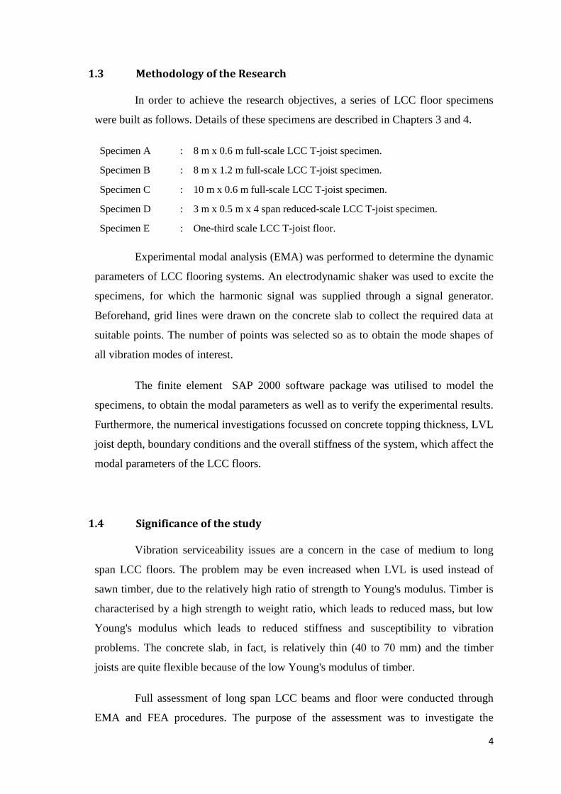
In order to achieve the research objectives, a series of LCC floor specimens
were built as follows. Details of these specimens are described in Chapters 3 and 4.
Specimen A : 8 m x 0.6 m full-scale LCC T-joist specimen.
Specimen B : 8 m x 1.2 m full-scale LCC T-joist specimen.
Specimen C : 10 m x 0.6 m full-scale LCC T-joist specimen.
Specimen D : 3 m x 0.5 m x 4 span reduced-scale LCC T-joist specimen.
Specimen E : One-third scale LCC T-joist floor.
Experimental modal analysis (EMA) was performed to determine the dynamic
parameters of LCC flooring systems. An electrodynamic shaker was used to excite the
specimens, for which the harmonic signal was supplied through a signal generator.
Beforehand, grid lines were drawn on the concrete slab to collect the required data at
suitable points. The number of points was selected so as to obtain the mode shapes of
all vibration modes of interest.
The finite element SAP 2000 software package was utilised to model the
specimens, to obtain the modal parameters as well as to verify the experimental results.
Furthermore, the numerical investigations focussed on concrete topping thickness, LVL
joist depth, boundary conditions and the overall stiffness of the system, which affect the
modal parameters of the LCC floors.
1.4 Significance of the study
Vibration serviceability issues are a concern in the case of medium to long
span LCC floors. The problem may be even increased when LVL is used instead of
sawn timber, due to the relatively high ratio of strength to Young's modulus. Timber is
characterised by a high strength to weight ratio, which leads to reduced mass, but low
Young's modulus which leads to reduced stiffness and susceptibility to vibration
problems. The concrete slab, in fact, is relatively thin (40 to 70 mm) and the timber
joists are quite flexible because of the low Young's modulus of timber.
Full assessment of long span LCC beams and floor were conducted through
EMA and FEA procedures. The purpose of the assessment was to investigate the
5
dynamic behaviour of the LCC floor and to ensure the LCC floor met the vibration
serviceability limitation as suggested in Euro code 5 (CEN, 2005). Thus, the main
contributions of this research include:
1. The assessment was conducted with different span lengths of LCC beams.
The results show that the longest span for an LCC beam of the dimensions
tested in this thesis is 8 m as the fundamental natural frequency is more
than 8 Hz. The natural frequency for a 10 m beam was found to be less than
8 Hz. The greater deflection and rotation of the 10 m beam could be seen
during the experimental work. Thus, a 10 m beam floor is not
recommended unless larger LVL beams are used, possibly in conjunction
with a thicker concrete slab.
2. According to the parametric study on an 8m x 7.8 m LCC floor, a minimum
concrete topping thickness is proposed based on the standard size of LVL
joist from a manufacturer. For an LVL joist depth of 150 mm to 240 mm
with 63 mm breath, the minimum concrete thickness is 100 mm and for
LVL joist depth 300 mm to 400 mm with 63 mm breath, the minimum
concrete thickness is 65 mm. This is a guide for a designer to estimate the
size of LCC floor to meet the vibration serviceability limit.
3. A simple design method is recommended for controlling vibration based on
the vibration serviceability limit state. The design method is based on finite
element modelling (FEM). The FEM was better than hand calculation in
terms of time and difficulty, especially for complex structures.
1.5 Outline of Thesis
Eight chapters are used to present the research work in this thesis. A brief
summary of each chapter is discussed in this section.
This Chapter 1 gives a brief introduction to this research including the research
background, problems, and objectives and scope of the studies. The research was
focused on serviceability problems of LCC floors.
6
Chapter 2 discusses previous research results that focus on (1) timber-concrete
composite floor systems and (2) floor vibrations. The discussion begins with the
development of timber-concrete composite systems, including background details and
development of this system by other researchers. The connection between timber and
concrete becomes the most important part of the system. Thus, most of the studies
focus on the shear connectors, which are made from mechanical or adhesive fasteners.
Later, the discussions concentrate on the investigation of floor vibration,
including timber, steel, concrete and composite flooring systems. The design of
vibration control recommended for each type of flooring system will give guidance to
this research to generate a new guideline for vibration control of LCC flooring systems.
Chapter 3 represents a step by step preliminary study on dynamic performance
of full-scale LCC floors, including the vertical vibration methodology and data
analysis, which will give guidance to the investigations of the multi-span and multi-
storey reduced-scale LCC specimens. To verify the experimental data, finite element
modelling used the SAP 2000 software package to generate the predicted behaviour.
Comparisons between experimental and modelling investigations on dynamic
behaviour are discussed later in this chapter.
Chapter 4 describes detailed construction of reduced-scale LCC T-joist
specimens and LCC T-joist floors. The details were implemented from full-scale
specimens, where 4 spans of LCC T-joist specimens were built with 2.8 m span length
for each T-joist specimen. The four T-joist specimens were connected to each other
with timber blocks (which act as columns) and the concrete was poured on the top as a
continuous slab, to study the dynamic performance of multi-span behaviour. Later, the
4-span specimens were cut and stacked on top of each other to study the vibration
behaviour of a multi-storey building. To understand more about the vibration behaviour
on large scale flooring systems, a 3m x 3m simply supported floor T-joist floor built by
others was tested as part of this research programme. Later, Chapter 4 discusses the
results of the experimental investigation into reduced-scale LCC T-joist specimens and
LCC T-joist floors. The vibration parameters, including natural frequencies and
damping ratios of the principal modes of the specimens were obtained. Also, the
transmissibility of the vibration energy between spans and storeys was investigated,
with recommendations for design and construction of real buildings.
7
Chapter 5 discusses the correlation between finite element modelling and
forced vibration test results, including natural frequencies and damping ratios of the
principal modes of vibration. The vibration transmissibility between spans and storeys
was also investigated.
Chapter 6 discusses the dynamic behaviour of a full-scale 8 m x 7. 8 m LCC
floor. The floor was modelled using the SAP 2000 software package and the modelling
parameters were adopted from the previous model described in Chapter 4. The
investigations were expanded by changing some parameters, including different types
of boundary conditions, to get a better understanding of the vibration behaviour of these
systems.
Chapter 7 introduces new design proposals for limiting the vibrations of LCC
flooring systems, including a proposed step-by-step method to design the floor using
finite element software. This guide also presents what designers should have to know
and what not to do in the process of designing for the serviceability limit of LCC
flooring systems.
Chapter 8 summarises and concludes the complete work in this research
project. The recommendations for future research, which are mainly findings from this
project, are also provided in this chapter.
CHAPTER 2 LITERATURE REVIEW
This chapter discusses previous research that focused on timber-concrete
composite (TCC) floor systems, and floor vibration. The discussion begins with the
development of timber-concrete, including background details and development of this
system by a number of researchers. The connection between timber and concrete is the
most important part of the system, thus, most of the studies focus on the shear
connectors, which are made from mechanical or adhesive fasteners. The new system of
TCC by replacing traditional timber joists by laminated veneer lumber (LVL) was
introduced by Yeoh (2008), known as an LVL-concrete composite (LCC) floor in this
study, is also discussed in this chapter.
Later, the discussions concentrate on the investigation of floor vibration,
including timber, steel, concrete and composite flooring systems. The design limitations
for vibration control for each type of flooring system are used to generate a new
guideline for LCC flooring systems
2.1 Timber-concrete composite (TCC) floor system
TCC floors are an efficient system to replace the traditional flooring systems.
This system has improved the stiffness of the floors and can fulfil the latest
requirements for flooring systems which require long spans and lightweight systems
(Natterer et.al., 1996). TCC floor systems are a hybrid between concrete and timber
adopted from stressed skin floor systems, where the upper timber flanges are replaced
with concrete. This system requires shear connectors to transfer forces from the
concrete slab to the timber joists. (Ceccotti, 1995) explained that timber-concrete
composite structures represent a construction technique that can be used for both
strength and stiffness upgrading of existing timber floors as well as in new buildings.
This technique connected a solid or glued laminated timber beam with a concrete slab
cast above, and included shear connectors to resist differential movement between the
timber and concrete.
9
The coupling of a concrete layer on the compression side and a timber beam
on the tension side of the composite cross section makes use of the advantageous
properties of these materials in terms of strength and stiffness. In this way an effective
structure characterized by relatively low weight can be obtained (Stojić and Cvetković,
2001). The idea of using concrete and timber in a composite cross-section is a natural
extension of an old technique, and it is even possible to attain full composite action if
‘non-slip’ connections are used.
The combination of the concrete and timber gave extra advantages that
produced a structurally efficient section, rigid and light at the same time. Additionally,
composite systems can have triple the load-carrying capability and up to six times the
flexural rigidity of traditional timber floor systems, if the timber and concrete are well
connected. A concrete topping increases the stiffness and strength of the floors, and can
be used to construct up to 15 m long-span flooring systems. (Ceccotti, 1995).
The advantages of the TCC systems and comparison between reinforced
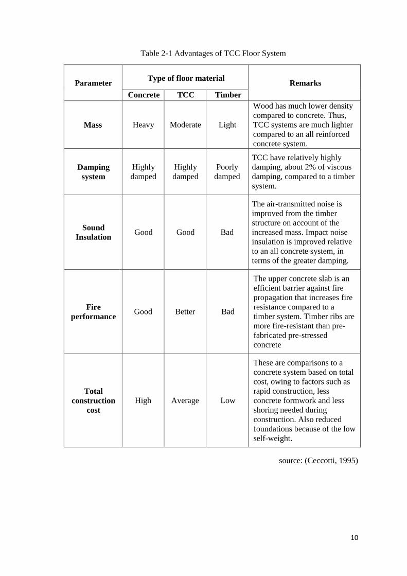
concrete and timber only systems are summarised in Table 2-1.
10
Table 2-1 Advantages of TCC Floor System
Parameter Type of floor material
Remarks
Concrete TCC Timber
Mass Heavy Moderate Light
Wood has much lower density
compared to concrete. Thus,
TCC systems are much lighter
compared to an all reinforced
concrete system.
Damping
system
Highly
damped
Highly
damped
Poorly
damped
TCC have relatively highly
damping, about 2% of viscous
damping, compared to a timber
system.
Sound
Insulation Good Good Bad
The air-transmitted noise is
improved from the timber
structure on account of the
increased mass. Impact noise
insulation is improved relative
to an all concrete system, in
terms of the greater damping.
Fire
performance Good Better Bad
The upper concrete slab is an
efficient barrier against fire
propagation that increases fire
resistance compared to a
timber system. Timber ribs are
more fire-resistant than pre-
fabricated pre-stressed
concrete
Total
construction
cost
High Average Low
These are comparisons to a
concrete system based on total
cost, owing to factors such as
rapid construction, less
concrete formwork and less
shoring needed during
construction. Also reduced
foundations because of the low
self-weight.
source: (Ceccotti, 1995)
11
2.1.1 Development of TCC
The development of TCC has focused on shear connectors between the timber
and concrete topping. Ample research has been done to improve solutions for this
connection system. The earliest development of the timber and concrete composite
system dates back to the 1920’s and 1930’s. The systems were initially developed in
Europe in 1929 when Mueller patented a system of nails and steel braces that formed
the connection between a concrete slab and the timber, and in 1939, Schwab applied for
a patent on timber-concrete composite components as mentioned by Seibold (2004) in
her literature.
The development of TCC in Europe expanded in 1985 when Sprig introduced
a new type of connector made of a doubled-headed screw. Another fastener was
invented in 1992 by Provis using a special screw. The screw had a special thread on the
lower part to allow for placement in the timber girder without having to drill a pilot
hole first and the smooth upper shaft was anchored into the concrete. In 1993, Blaβ
introduced several types of mechanical fasteners for TCC construction; (a) mechanical
fasteners with pin-shaped joints, (b) mechanical fasteners with special connectors and
(c) adhesive fasteners to create form closure. A new innovation of timber-concrete
composite systems called the HBV-system in 2000 was introduced by Bathon with
steel plates as a connector between the timber and concrete as reported by HBV-
Systeme (2003).
Lukaszewska et.al (2006) and Lukaszewska (2009) tested different types of
connectors to prevent the slip behaviour on the timber-concrete composite floor. The
proposed connectors were (1) nail plate, (2) continuous steel mesh, (3) a set of 2 steel
tubes with 20 mm diameter screw, (4) bent steel plate with nails, (5) bent steel plate
with epoxy glued, (6) a set of steel tube with 20 mm diameter screw and notch in the
joist and (7) 20 mm diameter dowels with flanges. The wooden shear anchor-keys with
inclined nails were developed by Crocetti et. al (2010) as a connecter for timber-
concrete composite floors, which attached to the timber joist by glue or screws. Crocetti
et al. (2015) added extra screws at both sides of the wooden anchor-keys. The functions
of the screws were to get the proper anchorage of the shear anchor-key to the concrete
topping and to reduce the risk of the anchor-key splitting as the specimen was loaded.
12
The development of a composite system using steel connectors was carried out
at the University of Oregon, USA in 1930 (Benitez, 2000). Unlike Europe, where the
composite systems developed because of renovating historical timber floors, in the
USA, they focused more on low to medium rise construction. Work at Colorado State
University by Gutkowski et. al. (2000) adopted a connection detail using notched
shear keys with anchors in the timber-concrete composite floor system, which was
proposed by (Natterer et.al., 1996).
New Zealand introduced a composite system for bridges around 1970 (Nauta,
1970). Glulam was used as beams in conjunction with 150 mm thick concrete slabs for
heavy duty traffic loads.
As mentioned previously, mechanical fasteners were used widely to tie
together concrete slabs and timber joists. However, alternative products such as
adhesives have been produced, which are capable of bonding the concrete both in wet
and hardened conditions which create slip-free connections and decrease beam
deflections (Brunner et al., 2007).
There is still strong uncertainty on the effectiveness of using a glued interface
between the concrete slab and the timber beam, although some research has been
carried out and presented (Brunner et al. (2007) and Hehl et al. (2014) ). However there
is no research proving that the glued interface will remain effective in the long-term -
therefore there is concern about using a pure glued interface between the concrete slab
and the timber beam, not only due to thermal strains and stresses, but also due to
possible moisture variations in the timber, and drying shrinkage of the concrete slab
which may produce problems (e.g. detachment) in the long-term.
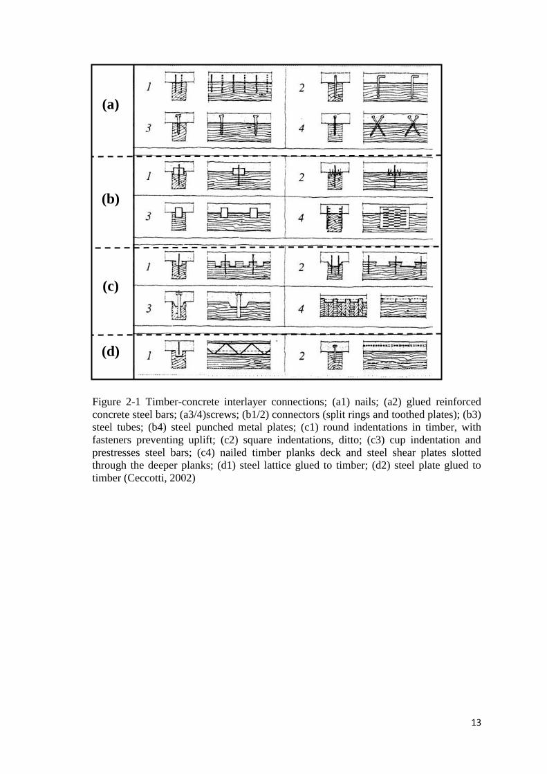
The relationship between the mechanical fasteners with their stiffness was
summarized in Figure 2-1 which, (Ceccotti, 2002), range from the less stiffness
connection (group a) to the stiffest connection (group d). Connections in group (a), (b)
and (c) permit relative slip between concrete and timber, i.e cross-sections do not
remain planar under load. Only connections in group (d) maintain planarity. Roughly
speaking, systems with group (a) connections achieve 50% of the bending stiffness of
systems with group (d) connections. The latter corresponds to fully composite action.
13
Figure 2-1 Timber-concrete interlayer connections; (a1) nails; (a2) glued reinforced
concrete steel bars; (a3/4)screws; (b1/2) connectors (split rings and toothed plates); (b3)
steel tubes; (b4) steel punched metal plates; (c1) round indentations in timber, with
fasteners preventing uplift; (c2) square indentations, ditto; (c3) cup indentation and
prestresses steel bars; (c4) nailed timber planks deck and steel shear plates slotted
through the deeper planks; (d1) steel lattice glued to timber; (d2) steel plate glued to
timber (Ceccotti, 2002)
(a)
(b)
(c)
(d)
14
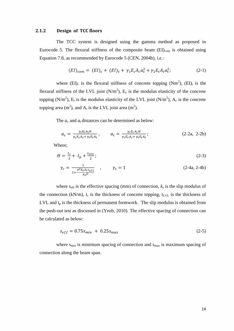
2.1.2 Design of TCC floors
The TCC system is designed using the gamma method as proposed in
Eurocode 5. The flexural stiffness of the composite beam (EI)com is obtained using
Equation 7.8, as recommended by Eurocode 5 (CEN, 2004b), i.e.:
(2-1)
where (EI)c is the flexural stiffness of concrete topping (Nm2), (EI)t is the
flexural stiffness of the LVL joist (N/m2), Ec is the modulus elasticity of the concrete
topping (N/m2), Et is the modulus elasticity of the LVL joist (N/m
2), Ac is the concrete
topping area (m2), and At is the LVL joist area (m
2).
The ac and at distances can be determined as below:
(2-2a, 2-2b)
Where;
(2-3)
(2-4a, 2-4b)
where seff is the effective spacing (mm) of connection, ks is the slip modulus of
the connection (kN/m), tc is the thickness of concrete topping, tLVL is the thickness of
LVL and tp is the thickness of permanent formwork. The slip modulus is obtained from
the push-out test as discussed in (Yeoh, 2010). The effective spacing of connection can
be calculated as below:
(2-5)
where smin is minimum spacing of connection and smax is maximum spacing of
connection along the beam span.

15
2.1.3 LVL-Concrete Composite Flooring System
The TCC flooring system as mentioned before is a sandwich of concrete (as a
slab) and timber (as a joist). The timber joist used is usually solid sawn timber. To
improve the system strength, glued laminated (Glulam) timber was used to replace the
solid timber (Van der Linden, 1999). However, he found that the engineered wood
material, laminated veneer lumber (LVL), was designed to get better strength and
material properties compared to Glulam. LVL also used widely in New Zealand and
Australia, thus, in this research, LVL was used to replaced traditional solid timber or
glued laminated (Glulam) timber joist in an LVL-Concrete Composite (LCC) flooring
system.
LVL is made from rotary peeled timber veneers which are glued together
using a durable adhesive and laid up with parallel grain orientation to form a
continuous billet, up to 12 m long and 1.2 m wide, usually having a thickness of 45, 63
or 90 mm. Solid and Glulam timber have larger coefficients of variation for both
strength (modulus of rupture) and stiffness (modulus of elasticity) compared to LVL,
which is very strong (almost three times the strength of sawn timber), more reliable and
with a higher modulus of elasticity (about 1.5 times the MOE of sawn timber) (Abd
Ghafar, 2008).
Researchers at the University of Canterbury in Christchurch, New Zealand
have collaborated with Carter Holt Harvey Wood products, local LVL manufacturers
and developed an experimental programme aimed at producing a semi-prefabricated
LCC floor system for Australasian market demands. The programme started when
Seibold (2004) studied the performance of LVL used as joist members in LCC systems,
and investigated the best shear connection of the system. Seibold (2004) studied a
series of different types of timber concrete composite connectors and found that the
best performance in shear was obtained using a specimen with notched joists and coach
screws, which resulted in high stiffness connections.
Gross (2004) used LCC beams with the connector suggested by Seibold (2004)
to determine the stiffness and strength of the system for use in long-span flooring
applications. The beams were built in three different cases; (a) lightweight concrete
with a strong shear connection, (b) pre-stressing the composite system beam with a
16
straight tendon using a strong shear connection, and (c) a pre-stressed beam with a
draped tendon and a weaker shear connection. The results showed that the composite
beam stiffness was increased sufficiently.
Furthermore, Yeoh (2008, 2010) continued the study to optimise the notch
geometry, both in mechanical and economical terms. He found that the best types of
connectors for LCC flooring systems were (a) a 300 mm long rectangular notch cut in
the LVL-joist and reinforced with a 16 mm diameter coach screw, (b) a triangular notch
reinforced with the same coach screw, and (c) two 333 mm long toothed metal plates,
pressed into the edges of the LVL joists.
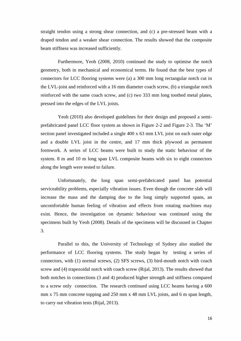
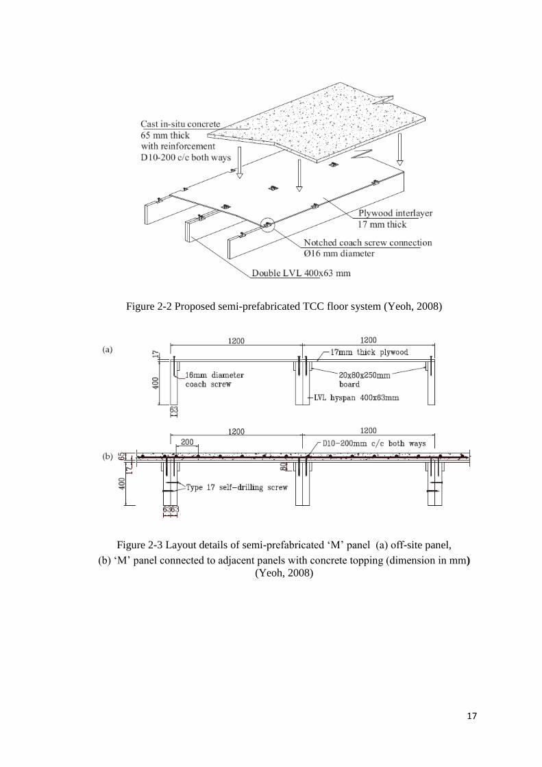
Yeoh (2010) also developed guidelines for their design and proposed a semi-
prefabricated panel LCC floor system as shown in Figure 2-2 and Figure 2-3. The ‘M’
section panel investigated included a single 400 x 63 mm LVL joist on each outer edge
and a double LVL joist in the centre, and 17 mm thick plywood as permanent
formwork. A series of LCC beams were built to study the static behaviour of the
system. 8 m and 10 m long span LVL composite beams with six to eight connectors
along the length were tested to failure.
Unfortunately, the long span semi-prefabricated panel has potential
serviceability problems, especially vibration issues. Even though the concrete slab will
increase the mass and the damping due to the long simply supported spans, an
uncomfortable human feeling of vibration and effects from rotating machines may
exist. Hence, the investigation on dynamic behaviour was continued using the
specimens built by Yeoh (2008). Details of the specimens will be discussed in Chapter
3.
Parallel to this, the University of Technology of Sydney also studied the
performance of LCC flooring systems. The study began by testing a series of
connectors, with (1) normal screws, (2) SFS screws, (3) bird-mouth notch with coach
screw and (4) trapezoidal notch with coach screw (Rijal, 2013). The results showed that
both notches in connections (3 and 4) produced higher strength and stiffness compared
to a screw only connection. The research continued using LCC beams having a 600
mm x 75 mm concrete topping and 250 mm x 48 mm LVL joists, and 6 m span length,
to carry out vibration tests (Rijal, 2013).
17
Figure 2-2 Proposed semi-prefabricated TCC floor system (Yeoh, 2008)
Figure 2-3 Layout details of semi-prefabricated ‘M’ panel (a) off-site panel,
(b) ‘M’ panel connected to adjacent panels with concrete topping (dimension in mm)
(Yeoh, 2008)
18
2.2 Floor Vibration
The vibration serviceability problem of the floor has been a concern since the
early 19th
century when in 1828 Tredgold stated that girders over long spans should be
deep to avoid the inconvenience of not being able to move on the floor without shaking
everything in the room (Allen and Murray, 1993). Since then, floor vibrations have
been studied in order to determine the vibration behaviour due to human-induced loads
and methods to prevent uncomfortable vibration on floors.
These days, the vibration serviceability problem of a floor due to decreased
floor mass and longer span lengths as demanded in a large variety of construction using
long span floors. The vibration on floors happens due to cyclic motion which repeats
itself, in particular over a certain interval of time, and affects its occupants during the
course of their normal human activities.
The activities that cause the serviceability problem are categorised as those
due to continuous vibration or to transient vibrations. Human group activities such as
dancing or jumping, or from the use of machinery, produce periodic forces and cause
continuous vibration. If a periodic force has similar frequency to the natural frequency
of the structure, the amplitude of the resultant motion is increased significantly, leading
to the condition known as resonance. Impact force from human activities such as
walking can generate transient vibrations. Such motion decays in propagation due to the
available damping in the structural system.
A vibration can be translated into six degrees of freedom (DOF), of which
three are translations and three are rotations through the centre of gravity in the x, y and
z axes. The translational motions produce stresses due to bending, which translate as
mode shapes from a vibration point of view. The research in this thesis only focuses on
translational vibration behaviour.
19
2.2.1 Floor Vibration Assessment
The vibration serviceability problem can be determined by investigating the
vibration behaviour of the floor, such as the natural frequency and damping ratio. To
get the vibration behaviour, the floor should be examined by experimental testing or
finite element analysis. The earliest experimental work was performed by Tilden (1913)
and Fuller (1924). Both studied the dynamic loads due to group activities on the floors.
Tilden (1913) also investigated the effect of an individual person on the floor. The
transient vibration problem was studied by exposing a group of persons to vertical and
horizontal vibrations while standing on a platform as discussed by Reiher and Meister
(1931), and Lenzen (1966) to investigate the damping performance of the floor.
Testing was performed by Wiss and Parmelee (1974) to propose a rating factor
as a function of the initial amplitude, the vibration frequency and the damping ratio. For
this work, individuals were asked to rate their perceptions while standing and being
seated on the floor in order to evaluate the human sensitivity due to transient vibration.
Nelson (1974) also recommended using a rating curve, but with a greater damping ratio
of the floor compared with the Wiss and Parmelee (1974) rating curve.
Later, the force platform was used to study the effect of human activities in a
group. Tuan and Saul (1985) investigated a group of persons in a weight range from 52
kg to 98 kg simulating crowd movement in a stadium and proposed that a narrow-band
live load spectrum with rhythmic jumping should be included when designing the
serviceability of the floor system under these conditions. Ebrahimpour and Sack (1989
& 1992) and Ebrahimpour et. al (1996) measured the force imposed by individuals and
groups of two and four people. A simplified expression for dynamic loads and a
footstep frequency for walking tests were suggested of 1.5, 1.75, 2.0 and 2.5 Hz.
The heel-drop test was developed by Lenzen (1966) to simulate a worst case
transient event. This method was the simplest of the excitation methods, where a person
stood in the middle of the floor, on the load cell platform, rose onto their toes and then
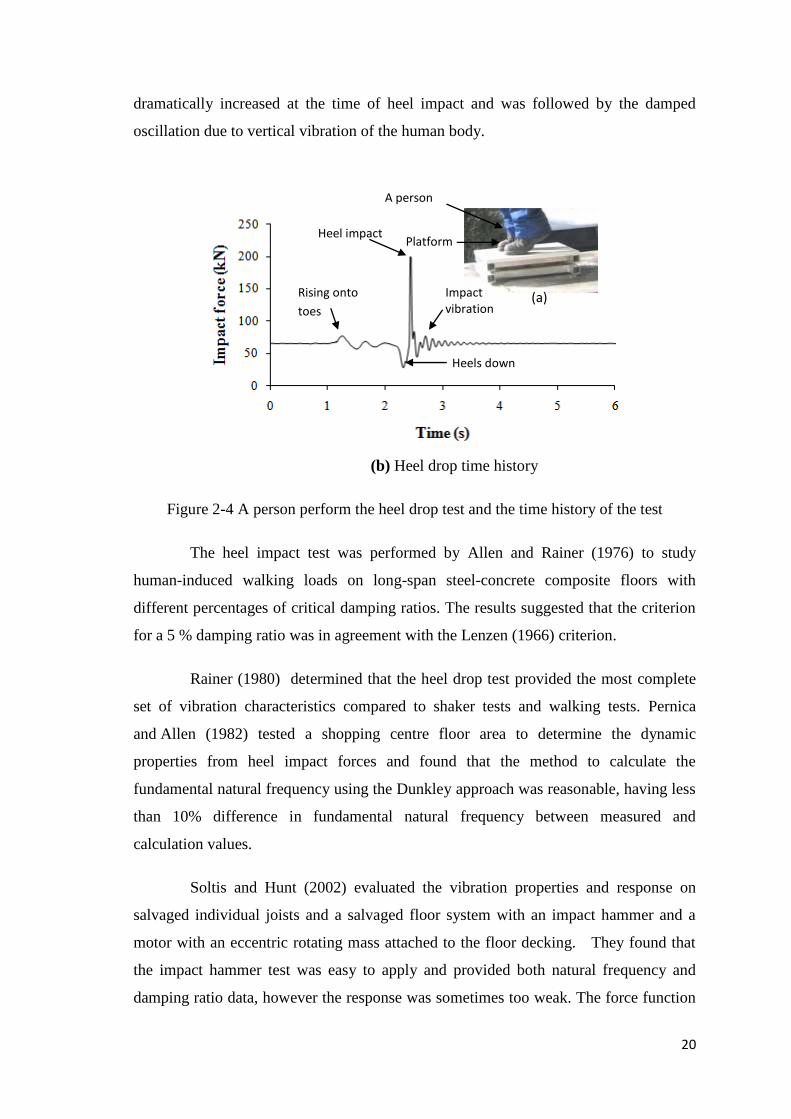
dropped down so that their heels struck the floor (Blakeborough and Williams, 2003).
The typical heel drop response is illustrated in Figure 2-4. The moment the
person rose to their toes from the normal position, a small fluctuation appears until the
initial reduction in vertical force occurs when the heel comes down. The force
20
dramatically increased at the time of heel impact and was followed by the damped
oscillation due to vertical vibration of the human body.
(b) Heel drop time history
Figure 2-4 A person perform the heel drop test and the time history of the test
The heel impact test was performed by Allen and Rainer (1976) to study
human-induced walking loads on long-span steel-concrete composite floors with
different percentages of critical damping ratios. The results suggested that the criterion
for a 5 % damping ratio was in agreement with the Lenzen (1966) criterion.
Rainer (1980) determined that the heel drop test provided the most complete
set of vibration characteristics compared to shaker tests and walking tests. Pernica
and Allen (1982) tested a shopping centre floor area to determine the dynamic
properties from heel impact forces and found that the method to calculate the
fundamental natural frequency using the Dunkley approach was reasonable, having less
than 10% difference in fundamental natural frequency between measured and
calculation values.
Soltis and Hunt (2002) evaluated the vibration properties and response on
salvaged individual joists and a salvaged floor system with an impact hammer and a
motor with an eccentric rotating mass attached to the floor decking. They found that
the impact hammer test was easy to apply and provided both natural frequency and
damping ratio data, however the response was sometimes too weak. The force function
Heel impact
Impact vibration
Heels down
Rising onto
toes
Platform
(a)
A person
raises the toes
21
gave a stronger response and a more consistent result, but no damping ratio could be
obtained.
As the technology has grown with time, the vibration behaviour on floors is no
longer solely dependent on dynamic testing, and finite element modelling has been
conducted to evaluate experimental data. Pavic and Reynolds (2003) performed vertical
force excitation testing using an electrodynamic shaker and calibrated the response with
finite element modelling.
The preliminary finite element modelling was developed to predict the
vibration characteristics compared to judgement based on experience. El-Dardiry and Ji
(2006) created a 3-D model for isotropic and orthotropic flat plates for steel-composite
flooring systems and determined that the isotropic flat floor model was more accurate
than the orthotropic flat floor model.
2.2.2 Vibration Assessment on Timber-Concrete Composite (TCC) Floor
Bernard (2003) performed a series of dynamic tests on TCC floors. The
research concentrated on the influences of concrete thickness, plywood thickness, joist
size and spacing and also the specimen length. The impact hammer test and walking
test were carried out to determine the vibration behaviour according to the research
needs. As a result, Bernard found that the stiffness of the system had a major influence
on the natural frequency and damping ratio.
Bernard (2008) continued his research on lightweight Engineered Timber
Floors (ETF) and performed 5 series of laboratory tests which concentrated on common
design parameters (use of glue, nails and blocking), the effect of the joist spacing, span
and lumped mass at the mid-span of the floor, and the effect of the post-tensioning with
rubber inserts to improve the floor vibration response. The design features and the
proposed remedy to improve floor vibration behaviour were found to be largely
ineffective.
ARUP (2012) and Franklin and Hough (2014) performed the impact and
footfall induced test on a 3 bay x 5 bay TCC office floor in Nelson Marlborough
Institute of Technology (NMIT). The study points out that some local areas of floor
22
plate close to openings are predicted to exhibit potential vibration levels that exceed the
comfort criterion for typical offices. In addition, the damping was estimated from the
impact hammer test to be in the range 2.0 % to 3.0 %. The suggestion for modelling
was 2.0 % damping.
Rijal (2013) conducted the impact hammer test on 6 m TCC beams and a 6 m
and a 8 m timber floor module. The timber floor module was built using hySPAN
cross-banded LVL as the top flange and hySPAN PROJECT LVL as the webs and
bottom flanges. The natural frequencies for both floors were found to be more than 10
Hz, and influenced by material properties, shear connectors, moisture content, bouncing
at the supports and the boundary condition.
Skinner et al. (2013) studied the influences of concrete topping for upgrading a
timber floor. The concrete topping increased the stiffness of an existing timber floor
whilst minimising the load added to the existing structure and the change to the finished
floor to ceiling height. The thickness of concrete topping suggested was between 0 to
100 mm. Skinner (2013) determined the optimum thickness of concrete topping on an
TCC floor, suggesting that 20 mm thickness of concrete topping was sufficient to
increase the bending stiffness and improve the transient vibration response.
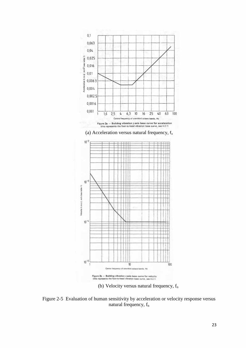
2.2.3 Human Perception of Floor Vibration
The human perception of floor vibration is very complex and difficult to
measure due to every person having their own perception. According to Ohlsson
(1988), the three most important parameters for human perception of vibration are the
duration, the activities on the floor, and the relative locations of the source and the
affected human person.
The evaluation of human response can be evaluated using a base curve as
shown in Figure 2-5 as recommended by ISO (ISO 2631-2:1989). The sensitivity of
human perception on the floor vibration can be evaluated by acceleration or velocity
responses to fundamental natural frequency, fn as illustrated in Figure 2-5 (a) and
Figure 2-5(b), respectively.
23
(a) Acceleration versus natural frequency, fn
(b) Velocity versus natural frequency, fn
Figure 2-5 Evaluation of human sensitivity by acceleration or velocity response versus
natural frequency, fn
24
2.2.4 Design Criteria for Floor Vibration
Traditional standards are recommended for evaluating the vibration of floors
according to the maximum deflection at the mid-span of the floors, as a span to length
ratio of 360. However, vibration design was neglected by only considering the static
stiffness, only guaranteeing by proxy that the vibration due to dynamic loads would not
be excessive. However, in some cases, this criterion was not satisfied because dynamic
loading produced by human or machinery influenced the floor and gave an annoying
feeling to the human subjects. Furthermore, the urban trends of buildings require longer
span floors to accommodate larger open spaces in residential and light commercial
construction. Thus, the design criteria to evaluate the vibrations of the floor have been
expanded using the fundamental natural frequency and response acceleration.
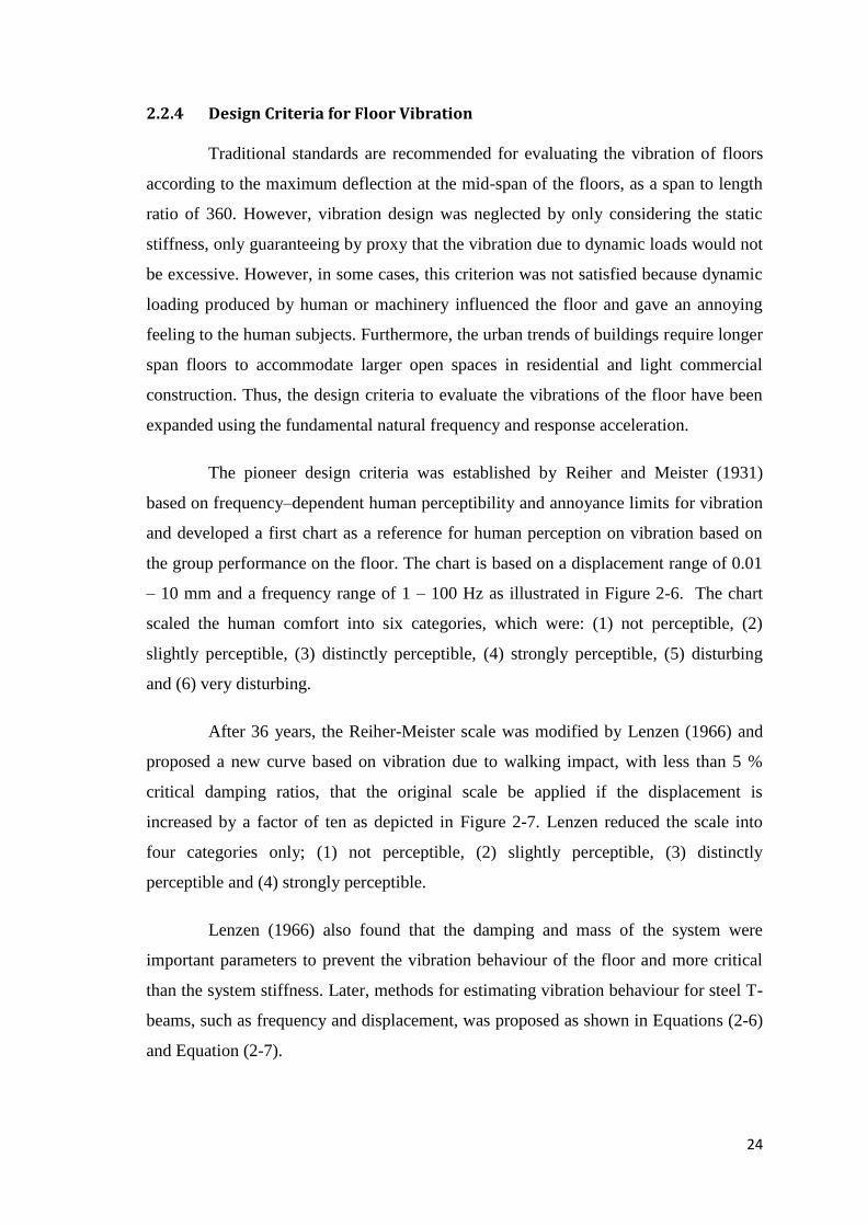
The pioneer design criteria was established by Reiher and Meister (1931)
based on frequency–dependent human perceptibility and annoyance limits for vibration
and developed a first chart as a reference for human perception on vibration based on
the group performance on the floor. The chart is based on a displacement range of 0.01
– 10 mm and a frequency range of 1 – 100 Hz as illustrated in Figure 2-6. The chart
scaled the human comfort into six categories, which were: (1) not perceptible, (2)
slightly perceptible, (3) distinctly perceptible, (4) strongly perceptible, (5) disturbing
and (6) very disturbing.
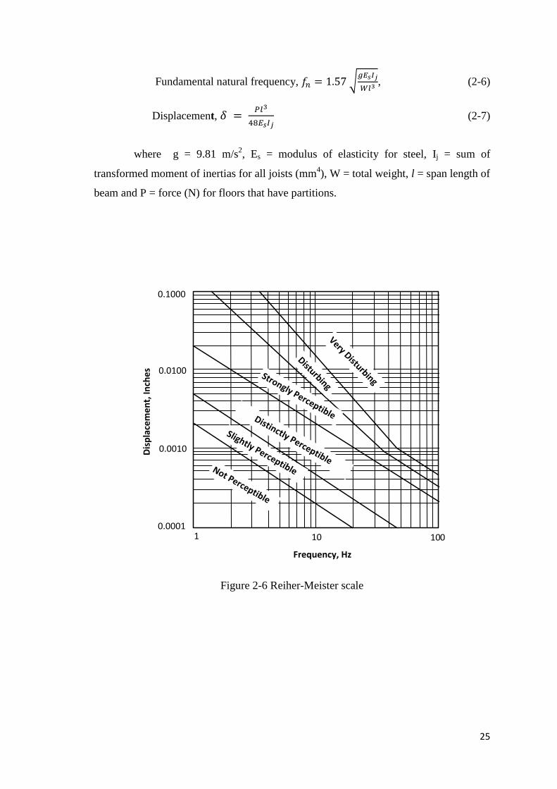
After 36 years, the Reiher-Meister scale was modified by Lenzen (1966) and
proposed a new curve based on vibration due to walking impact, with less than 5 %
critical damping ratios, that the original scale be applied if the displacement is
increased by a factor of ten as depicted in Figure 2-7. Lenzen reduced the scale into
four categories only; (1) not perceptible, (2) slightly perceptible, (3) distinctly
perceptible and (4) strongly perceptible.
Lenzen (1966) also found that the damping and mass of the system were
important parameters to prevent the vibration behaviour of the floor and more critical
than the system stiffness. Later, methods for estimating vibration behaviour for steel T-
beams, such as frequency and displacement, was proposed as shown in Equations (2-6)
and Equation (2-7).
25
Fundamental natural frequency,
, (2-6)
Displacement,
(2-7)
where g = 9.81 m/s2, Es = modulus of elasticity for steel, Ij = sum of
transformed moment of inertias for all joists (mm4), W = total weight, l = span length of
beam and P = force (N) for floors that have partitions.
0.1000
0.0100
0.0010
0.0001 1 10 100
Frequency, Hz
Dis
pla
cem
ent,
Inch
es
Disturbing
Very Disturbing
Strongly PerceptibleDistinctly Perceptible
Slightly PerceptibleNot Perceptible
Figure 2-6 Reiher-Meister scale
26
0.1000
0.0100
0.0010
1
10 100
Frequency, Hz
Dis
pla
cem
en
t, In
che
s
Strongly Perceptible
Distinctly Perceptible
Slightly PerceptibleNot Perceptible
Figure 2-7 Modified Reiher-Meister scale
Ohlsson (1988) created methodology to determine the vibration behaviour for
timber floors by limiting the impulse velocity response, h'max and static deflection.
However, this criterion was applicable only for timber floors with 8 Hz fundamental
natural frequency, or above. The impulse velocity response, h'max of simply supported
plates can be calculated as
(2-8)
where n40 is the modal number corresponding to 40 Hz,
Murray et al. (2003) proposed a design criterion to fulfil the human comfort.
The criterion states that the floor system is satisfactory if the peak acceleration, ap, due
to walking excitation as a fraction of the acceleration of gravity, g, determined from
( 2-9)
where Po is a constant force representing the excitation, fn is the fundamental
natural frequency of a joist panel, a beam panel or a combined panel as applicable, is
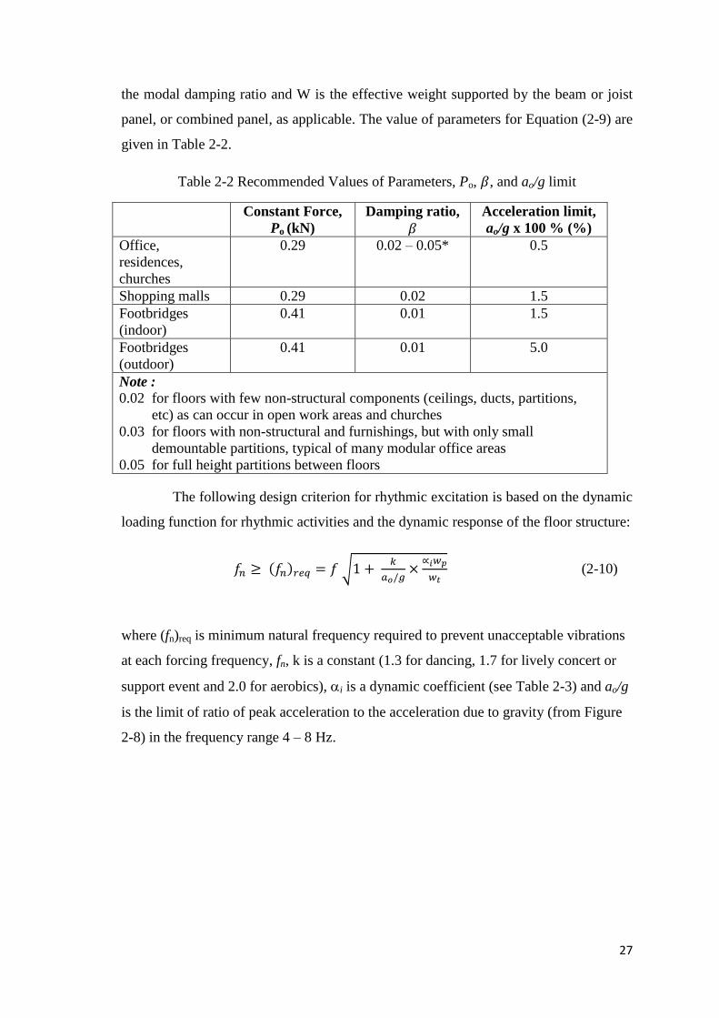
27
the modal damping ratio and W is the effective weight supported by the beam or joist
panel, or combined panel, as applicable. The value of parameters for Equation (2-9) are
given in Table 2-2.
Table 2-2 Recommended Values of Parameters, Po, , and ao/g limit
Constant Force,
Po (kN)
Damping ratio,
Acceleration limit,
ao/g x 100 % (%)
Office,
residences,
churches
0.29 0.02 – 0.05* 0.5
Shopping malls 0.29 0.02 1.5
Footbridges
(indoor)
0.41 0.01 1.5
Footbridges
(outdoor)
0.41 0.01 5.0
Note :
0.02 for floors with few non-structural components (ceilings, ducts, partitions,
etc) as can occur in open work areas and churches
0.03 for floors with non-structural and furnishings, but with only small
demountable partitions, typical of many modular office areas
0.05 for full height partitions between floors
The following design criterion for rhythmic excitation is based on the dynamic
loading function for rhythmic activities and the dynamic response of the floor structure:
(2-10)
where (fn)req is minimum natural frequency required to prevent unacceptable vibrations
at each forcing frequency, fn, k is a constant (1.3 for dancing, 1.7 for lively concert or
support event and 2.0 for aerobics), i is a dynamic coefficient (see Table 2-3) and ao/g
is the limit of ratio of peak acceleration to the acceleration due to gravity (from Figure
2-8) in the frequency range 4 – 8 Hz.
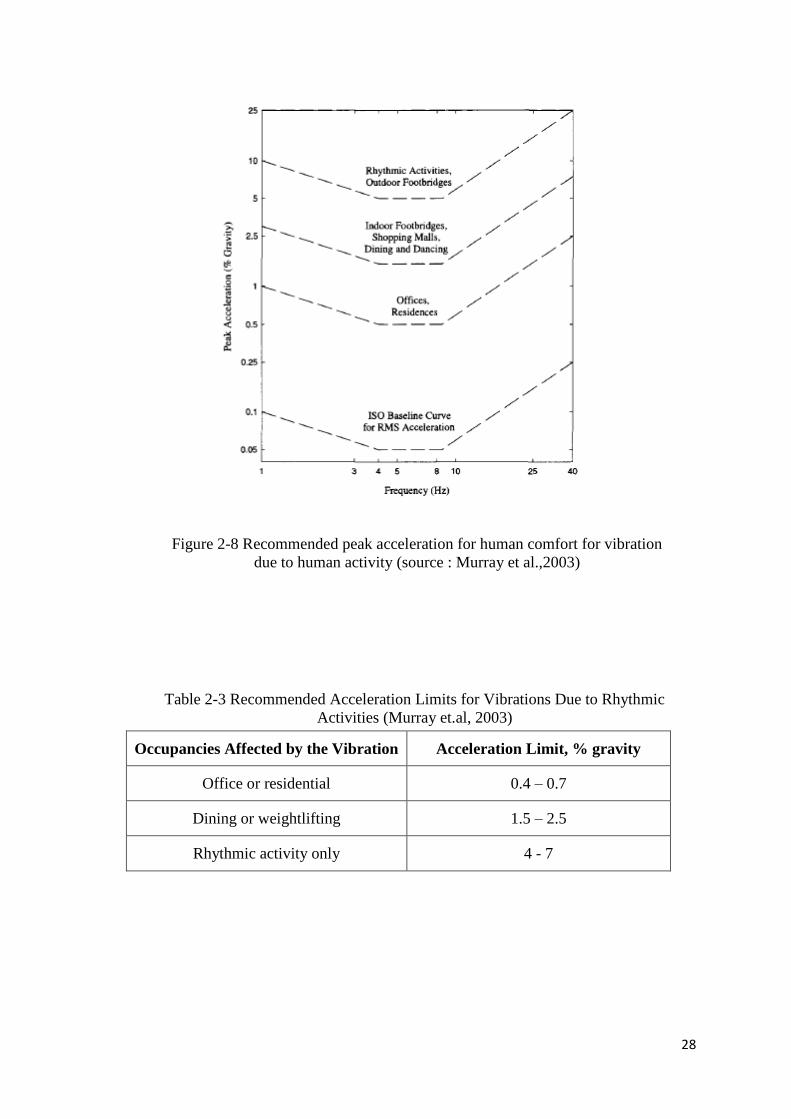
28
Figure 2-8 Recommended peak acceleration for human comfort for vibration
due to human activity (source : Murray et al.,2003)
Table 2-3 Recommended Acceleration Limits for Vibrations Due to Rhythmic
Activities (Murray et.al, 2003)
Occupancies Affected by the Vibration Acceleration Limit, % gravity
Office or residential 0.4 – 0.7
Dining or weightlifting 1.5 – 2.5
Rhythmic activity only 4 - 7
29
The static deflection recommended by Ohlsson, as published in the Swedish
Building Code, was for the deflection at midpsan to not exceed 1.5 mm when subjected
to a 1 kN point load. For a uniformly distributed load, the limitation of deflection can
be calculated as in Equation (2-11).
(2-11)
The equation of natural frequencies for rectangular orthotropic floors, simply
supported along all four edges, as in Equation (2-12) was adopted from Leissa (1969).
(2-12)
Ohlsson proposed a simplified equation to calculate fundamental natural
frequency as in Equation (2-13), for the low values of Dy/Dx (≤0.01) (Weckendorf,
2009).
(Hz) (2-13)
Hu (2007) proposed a new design criterion based on a 1 kN static deflection
and fundamental natural frequency for wood-framed timber floors. If the combination
of the calculated fundamental natural frequency, fn (Hz) and 1 kN static deflection, d
(mm) is larger than 18.7, then the floor is most likely acceptable to occupants in terms
of its vibration serviceability and vice versa. The design criterion equation was as
below:
(2-14)
or the simplified as
(2-15)
where the fundamental natural frequency, fn and static deflection, was
following ribbed-plate model as in Equation (2-16) and Equation (2-17).
30
(2-16)
(2-17)
where
(Nm) (system flexural rigidity in x-direction)
(Nm) (system flexural rigidity in y-direction)
(Nm) (Shear rigidity of multi-layered floor deck + torsion
ridigity of joist)
= mJ/b1 + s ts + c tc (kg/m2)
mJ = per unit length of joist (kg/m)
c = density of topping (kg/m3)
s = density of sub-floor (kg/m3)
tc = thickness of topping (m)
ts = thickness of sub-floor (m)
Gp = modulus of multi-layer floor deck (N/m2),
EIp = multi-layer floor deck EI (Nm),
EICJ = composite EI of joist (Nm2),
(EIb)i = ith lateral bracing member (Nm
2),
k = total number of rows of lateral bracing elements,
b1 = spacing of joist (m),
t = width of joist (m),
l = span of floor (m) and b is width of floor (m),
h = thickness of multi-layer floor topping (m),
H = height of floor system (joist depth + floor deck thickness (m)
C = joist torsional constant
31
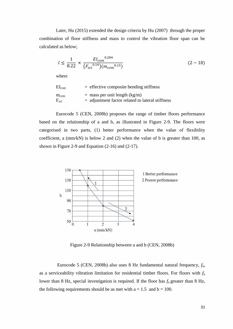
Later, Hu (2015) extended the design criteria by Hu (2007) through the proper
combination of floor stiffness and mass to control the vibration floor span can be
calculated as below;
where
EIcom = effective composite bending stiffness
mcom = mass per unit length (kg/m)
Fscl = adjustment factor related to lateral stiffness
Eurocode 5 (CEN, 2008b) proposes the range of timber floors performance
based on the relationship of a and b, as illustrated in Figure 2-9. The floors were
categorised in two parts, (1) better performance when the value of flexibility
coefficient, a (mm/kN) is below 2 and (2) when the value of b is greater than 100, as
shown in Figure 2-9 and Equation (2-16) and (2-17).
Figure 2-9 Relationship between a and b (CEN, 2008b)
Eurocode 5 (CEN, 2008b) also uses 8 Hz fundamental natural frequency, fn,
as a serviceability vibration limitation for residential timber floors. For floors with fn
lower than 8 Hz, special investigation is required. If the floor has fn greater than 8 Hz,
the following requirements should be as met with a = 1.5 and b = 100.
32
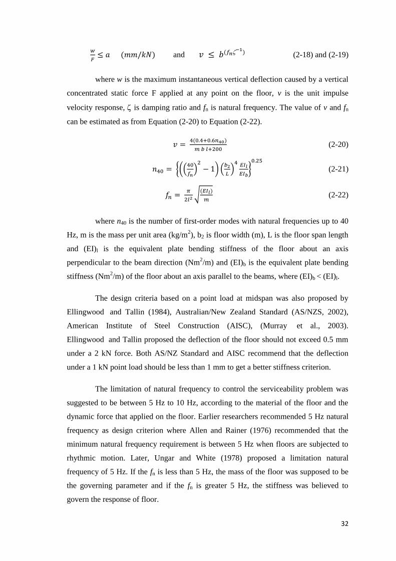
and
(2-18) and (2-19)
where w is the maximum instantaneous vertical deflection caused by a vertical
concentrated static force F applied at any point on the floor, v is the unit impulse
velocity response, is damping ratio and fn is natural frequency. The value of v and fn
can be estimated as from Equation (2-20) to Equation (2-22).
(2-20)
(2-21)
(2-22)
where n40 is the number of first-order modes with natural frequencies up to 40
Hz, m is the mass per unit area (kg/m2), b2 is floor width (m), L is the floor span length
and (EI)l is the equivalent plate bending stiffness of the floor about an axis
perpendicular to the beam direction (Nm2/m) and (EI)b is the equivalent plate bending
stiffness (Nm2/m) of the floor about an axis parallel to the beams, where (EI)b < (EI)l.
The design criteria based on a point load at midspan was also proposed by
Ellingwood and Tallin (1984), Australian/New Zealand Standard (AS/NZS, 2002),
American Institute of Steel Construction (AISC), (Murray et al., 2003).
Ellingwood and Tallin proposed the deflection of the floor should not exceed 0.5 mm
under a 2 kN force. Both AS/NZ Standard and AISC recommend that the deflection
under a 1 kN point load should be less than 1 mm to get a better stiffness criterion.
The limitation of natural frequency to control the serviceability problem was
suggested to be between 5 Hz to 10 Hz, according to the material of the floor and the
dynamic force that applied on the floor. Earlier researchers recommended 5 Hz natural
frequency as design criterion where Allen and Rainer (1976) recommended that the
minimum natural frequency requirement is between 5 Hz when floors are subjected to
rhythmic motion. Later, Ungar and White (1978) proposed a limitation natural
frequency of 5 Hz. If the fn is less than 5 Hz, the mass of the floor was supposed to be
the governing parameter and if the fn is greater 5 Hz, the stiffness was believed to
govern the response of floor.
33
The limitation of the natural frequency increased to higher than 5 Hz when
Allen (1985) produced a design procedure for rhythmic activities and suggested that the
minimum requirement for fundamental natural frequency is higher than 6 Hz. Smith
and Chui (1988) proposed the requirement that the fundamental frequency of vibration
for the floor is greater than 8 Hz. Wyatt (1989) recommended that the design criterion
of requiring the natural frequency to be greater than 7 Hz, but if the frequency is greater
than 9 Hz, the criterion becomes overly conservative because it ignores the benefits of
decreased decay time. Allen and Murray (1993) studied the effects of human induced
vibrations such as walking activities on steel floors and proposed that the natural
frequency for offices and residential system must be beyond 9 Hz to control impulse
vibration from footsteps based on harmonic resonance.
The Steel Construction Institute (SCI) 2nd Edition (Devine et. al, 2007)
classified the floor into two categories; (1) a low frequency floor if the fundamental
natural frequency was lower than 10 Hz and can be excited into resonance by walking,
and (2) a high frequency floor if the fundamental natural frequency is over 10 Hz for
general floors and the response to each individual is assumed to decay before the next
footfall.
In the United Kingdom, the traditional approach used to design conventional
composite floors for serviceability criteria has been to check the primary and secondary
beams independently for a minimum frequency of 4.0 Hz, and assuming that simply-
supported boundary conditions exist. Zivanovic and Pavic (2009) proposed a guideline
based on randomness in the walking force. The checking procedure is still based on
fundamental natural frequency and the cut-off frequency is 10 Hz. The floor was
considered to be prone to resonant vibration under walking-induced force if the
fundamental frequency is below 10 Hz. The human walking typically causes a transient
response to the heel impact each step if the fundamental frequency is over 10 Hz.
Human-imposed walking excitation was performed on four open-plan
classroom floors (9 m x 7 m) by Zivanovic and Pavic (2009). The testing protocol
followed was the Technical Report 43 (Appendix G), UK Concrete Society, and
brought to light a few drawbacks of the procedure. The floor cannot be classified as a
low- or high-frequency floor due to the non-negligible frequency content in the
measured response time history both below and above 10 Hz.

34
A summary of guidelines to control the vibration of timber floors is illustrated
in Table 2-4, from Hu (2015). The deflection criterion is mentioned in rows 1 to 3. The
floor deflection should be calculated under a uniformly distributed load or a 1 kN point
load as suggested by CCMC (1997) and NRC (2010). The limitation of natural
frequency in row 4, fn more than 14 Hz as proposed by Dolan et al. (1999) is very high
compared to 8 Hz as mentioned by Ohlsson (1988) Smith and Chui (1988) and many
others. Later, Table 2-5 gives a summary of many different standards introduced to
give some guidelines to limit the vibration for flooring systems, over the past 80 years
.
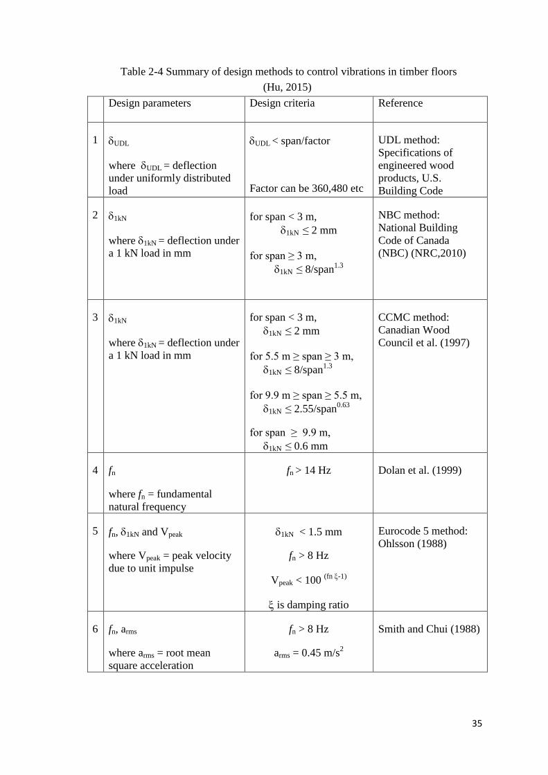
35
Table 2-4 Summary of design methods to control vibrations in timber floors
(Hu, 2015)
Design parameters
Design criteria Reference
1 UDL
where UDL = deflection
under uniformly distributed
load
UDL < span/factor
Factor can be 360,480 etc
UDL method:
Specifications of
engineered wood
products, U.S.
Building Code
2 1kN
where 1kN = deflection under
a 1 kN load in mm
for span < 3 m,
1kN ≤ 2 mm
for span ≥ 3 m,
1kN ≤ 8/span1.3
NBC method:
National Building
Code of Canada
(NBC) (NRC,2010)
3 1kN
where 1kN = deflection under
a 1 kN load in mm
for span < 3 m,
1kN ≤ 2 mm
for 5.5 m ≥ span ≥ 3 m,
1kN ≤ 8/span1.3
for 9.9 m ≥ span ≥ 5.5 m,
1kN ≤ 2.55/span0.63
for span ≥ 9.9 m,
1kN ≤ 0.6 mm
CCMC method:
Canadian Wood
Council et al. (1997)
4 fn
where fn = fundamental
natural frequency
fn > 14 Hz
Dolan et al. (1999)
5 fn, 1kN and Vpeak
where Vpeak = peak velocity
due to unit impulse
1kN < 1.5 mm
fn > 8 Hz
Vpeak < 100 (fn -1)
is damping ratio
Eurocode 5 method:
Ohlsson (1988)
6 fn, arms
where arms = root mean
square acceleration
fn > 8 Hz
arms = 0.45 m/s2
Smith and Chui (1988)
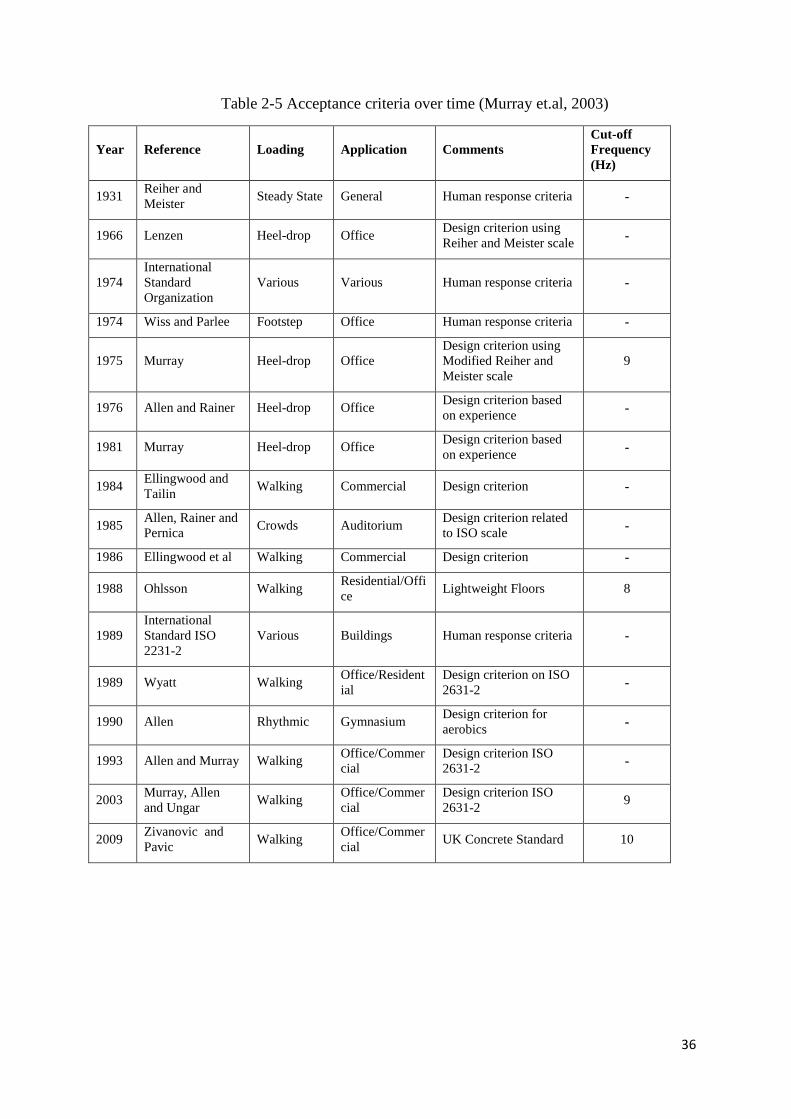
36
Table 2-5 Acceptance criteria over time (Murray et.al, 2003)
Year Reference Loading Application Comments
Cut-off
Frequency
(Hz)
1931 Reiher and
Meister Steady State General Human response criteria -
1966 Lenzen Heel-drop Office Design criterion using
Reiher and Meister scale -
1974
International
Standard
Organization
Various Various Human response criteria -
1974 Wiss and Parlee Footstep Office Human response criteria -
1975 Murray Heel-drop Office
Design criterion using
Modified Reiher and
Meister scale
9
1976 Allen and Rainer Heel-drop Office Design criterion based
on experience -
1981 Murray Heel-drop Office Design criterion based
on experience -
1984 Ellingwood and
Tailin Walking Commercial Design criterion -
1985 Allen, Rainer and
Pernica Crowds Auditorium
Design criterion related
to ISO scale -
1986 Ellingwood et al Walking Commercial Design criterion -
1988 Ohlsson Walking Residential/Offi
ce Lightweight Floors 8
1989
International
Standard ISO
2231-2
Various Buildings Human response criteria -
1989 Wyatt Walking Office/Resident
ial
Design criterion on ISO
2631-2 -
1990 Allen Rhythmic Gymnasium Design criterion for
aerobics -
1993 Allen and Murray Walking Office/Commer
cial
Design criterion ISO
2631-2 -
2003 Murray, Allen
and Ungar Walking
Office/Commer
cial
Design criterion ISO
2631-2 9
2009 Zivanovic and
Pavic Walking
Office/Commer
cial UK Concrete Standard 10
37
2.2.5 Use of Dampers to Control Floor Vibrations
The floor vibration problem could be improved by improving the stiffness, the
mass or the damping of the floor. However, changing the existing stiffness or mass of a
floor is not economical and satisfactory especially if it involves major retrofit
(Ljunggren, 2006). Another solution is to increase the damping by adding a non-
structural element on the floor or adding a mechanical damping device.
Mechanical damping devices (referred to as “dampers”) can reduce the
vibration problem and prevent discomfort from the floor vibration. Several methods or
types of damper are found, however, tuned mass dampers (TMD), active control, semi-
active tuned vibration absorbers and visco-elastic dampers are commonly reported, as
discussed by Ljunggren (2006). The earlier TMD had been developed by Lenzen
(1966), using a simple system of mass-spring-dashpot to synchronize the floor’s natural
frequency with the TMD’s natural frequency and hence dissipate the vibration energy.
The used of TMDs continued especially for lightweight floors (Bachmann & Ammann,
1987), gymnasiums (Thornton et. al, 1990), long-span floors (Webster and Vaicajtis,
1992)_and long-span balconies of auditoriums (Setareh and Hanson, 1992).
Later, a new TMD system introduced by Nguyen et al. (2012 and 2014) used
viscoelastic materials to control the vibration issues of real office floors. 12 TMDs were
applied on one bay of the office floor and walking and shaker tests were conducted to
study the vibration behaviour. The results show that the peak response was reduced
40% and the floor became acceptable from a human comfort perspective.
2.3 Summary
This chapter has reviewed the development of the timber-concrete composite
(TCC) floors and the previous studies on floor vibration, especially on assessment of
floors subjected to dynamic loads¸ and design guides to control the serviceability
vibration problem of floors.
The development of TCC concentrated on upgrading the stiffness of TCC's
connectors. The connectors suggested ranged from nails only to notches with screws.
The stiffness of the connector is important to prevent slip behaviour between the
38
concrete and timber. Furthermore, the traditional timber joist was replaced by LVL to
increase the strength of the floor since LVL has a higher strength compared to other
types of timber. However, the flexibility of the LVL was a concern when subjected to
dynamic loads.
The previous research showed that the natural frequency was one of the
important parameters that influenced the sensitivity of humans to dynamic floor
responses. The limitation of natural frequency was suggested to be from 5 Hz to 10 Hz,
according to the types of dynamic loads, and flooring material. However, in this
research, the limitation of natural frequency was focused on 8 Hz only after considering
the flexibility of LVL and the LCC flooring as designed for long-spans.
CHAPTER 3 FULL-SCALE LCC T-JOIST SPECIMENS
This chapter presents a comprehensive study on the dynamic performance of
full-scale LCC T-joist specimens including both experimental and finite element
simulation. Initially, the LCC T-joist specimen system is described together with past
experimental work by various researchers on LCC systems. The chapter follows with a
detailed investigation of the dynamic performance of the LCC flooring systems. This
preliminary investigation provides guidance for the subsequent investigation of
reduced-scale LCC T-joist specimens and floor as described in Chapters 4 and 5.
The investigation of the dynamic behaviour of LCC T-joist specimens was
carried out using an electrodynamic shaker. The shaker was placed on the top of the
specimens to conduct a vertical vibration test to determine the modal parameters of the
specimens, including natural frequencies, damping ratios and mode shapes. A signal
generator was connected to the electrodynamic shaker to generate the harmonic signal
and excite the specimens. Due to limited equipment, only a single harmonic signal was
applied, from 0 Hz to a maximum frequency, at 0.1 intervals, depending on resonance
of the specimens. Later, when a digital signal generator was available, a sweep signal,
from 2 Hz to 25 Hz, was used to verify the results from the single harmonic signal.
To process the experimental data, a signal processing software package known
as ME'scope was used. The data was processed using Fast Fourier Transform (FFT)
method and curve fitting method to determine the modal parameters (natural frequency,
damping ratio and mode shape).
A post-test numerical analysis was carried out using the Sap 2000 finite
element software package to compare with the experimental modal analysis (EMA)
results. The modelling was important because the similar modelling was expending to
analysis the full-scale LCC floor as discussed in Chapter 6.
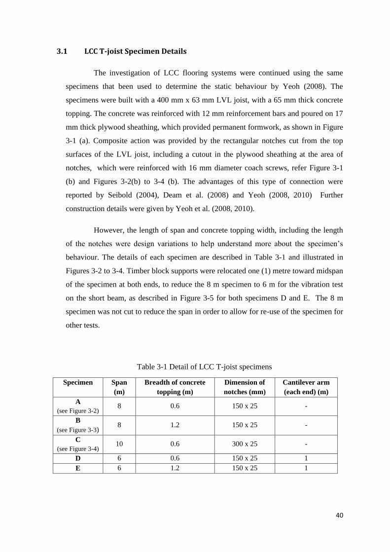
40
3.1 LCC T-joist Specimen Details
The investigation of LCC flooring systems were continued using the same
specimens that been used to determine the static behaviour by Yeoh (2008). The
specimens were built with a 400 mm x 63 mm LVL joist, with a 65 mm thick concrete
topping. The concrete was reinforced with 12 mm reinforcement bars and poured on 17
mm thick plywood sheathing, which provided permanent formwork, as shown in Figure
3-1 (a). Composite action was provided by the rectangular notches cut from the top
surfaces of the LVL joist, including a cutout in the plywood sheathing at the area of
notches, which were reinforced with 16 mm diameter coach screws, refer Figure 3-1
(b) and Figures 3-2(b) to 3-4 (b). The advantages of this type of connection were
reported by Seibold (2004), Deam et al. (2008) and Yeoh (2008, 2010) Further
construction details were given by Yeoh et al. (2008, 2010).
However, the length of span and concrete topping width, including the length
of the notches were design variations to help understand more about the specimen’s
behaviour. The details of each specimen are described in Table 3-1 and illustrated in
Figures 3-2 to 3-4. Timber block supports were relocated one (1) metre toward midspan
of the specimen at both ends, to reduce the 8 m specimen to 6 m for the vibration test
on the short beam, as described in Figure 3-5 for both specimens D and E. The 8 m
specimen was not cut to reduce the span in order to allow for re-use of the specimen for
other tests.
Table 3-1 Detail of LCC T-joist specimens
Specimen Span
(m)
Breadth of concrete
topping (m)
Dimension of
notches (mm)
Cantilever arm
(each end) (m)
A
(see Figure 3-2) 8 0.6 150 x 25 -
B
(see Figure 3-3) 8 1.2 150 x 25 -
C
(see Figure 3-4) 10 0.6 300 x 25 -
D 6 0.6 150 x 25 1
E 6 1.2 150 x 25 1
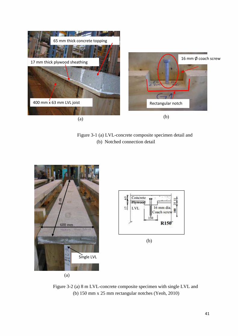
41
(a)
Figure 3-1 (a) LVL-concrete composite specimen detail and
(b) Notched connection detail
(a) (b)
600 mm
8 m
Single LVL
Figure 3-2 (a) 8 m LVL-concrete composite specimen with single LVL and
(b) 150 mm x 25 mm rectangular notches (Yeoh, 2010)
(a)
(b)
65 mm thick concrete topping
17 mm thick plywood sheathing
400 mm x 63 mm LVL joist
16 mm Ø coach screw
Rectangular notch
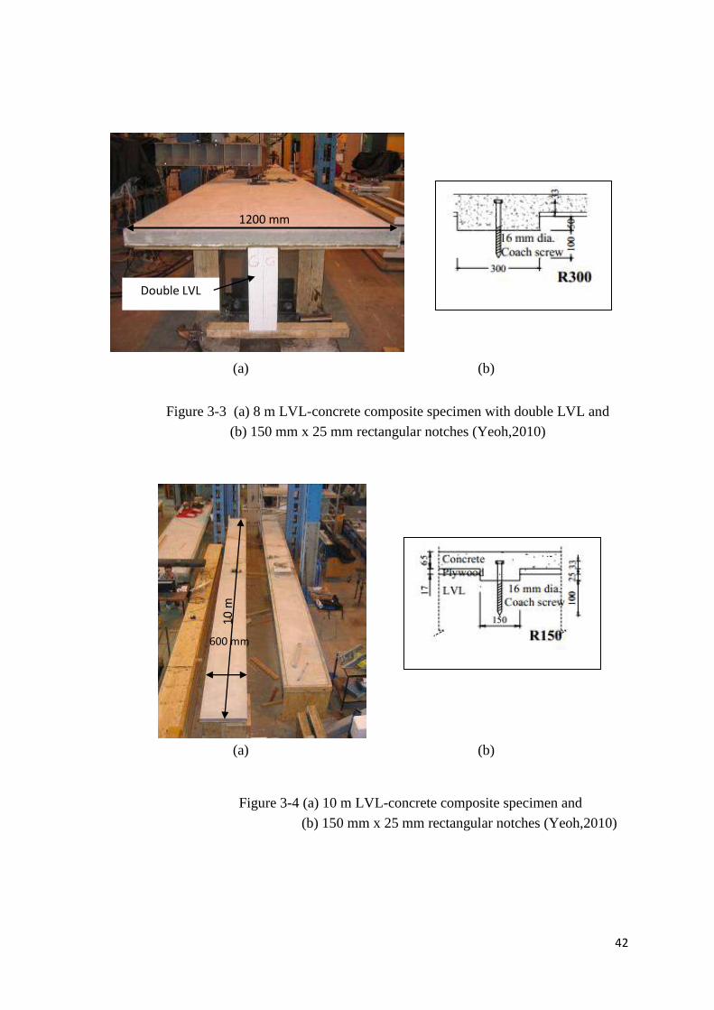
42
(a) (b)
(a) (b)
1200 mm
Double LVL
Figure 3-3 (a) 8 m LVL-concrete composite specimen with double LVL and
(b) 150 mm x 25 mm rectangular notches (Yeoh,2010)
600 mm
10
m
Figure 3-4 (a) 10 m LVL-concrete composite specimen and
(b) 150 mm x 25 mm rectangular notches (Yeoh,2010)
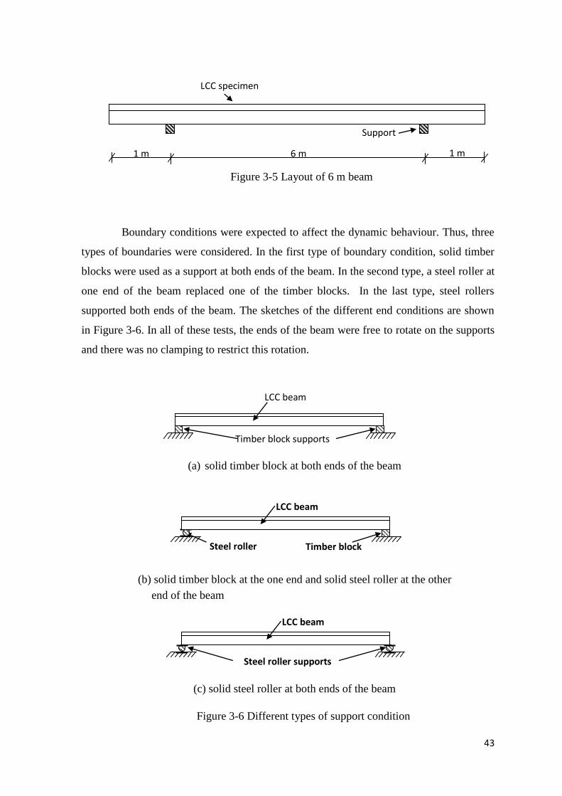
43
Boundary conditions were expected to affect the dynamic behaviour. Thus, three
types of boundaries were considered. In the first type of boundary condition, solid timber
blocks were used as a support at both ends of the beam. In the second type, a steel roller at
one end of the beam replaced one of the timber blocks. In the last type, steel rollers
supported both ends of the beam. The sketches of the different end conditions are shown
in Figure 3-6. In all of these tests, the ends of the beam were free to rotate on the supports
and there was no clamping to restrict this rotation.
(a) solid timber block at both ends of the beam
(b) solid timber block at the one end and solid steel roller at the other
end of the beam
(c) solid steel roller at both ends of the beam
Steel roller supports
LCC beam
Figure 3-6 Different types of support condition
Figure 3-5 Layout of 6 m beam
1 m
1 m
6 m
LCC specimen
Support
LCC beam
Timber block supports
LCC beam
Timber block Steel roller
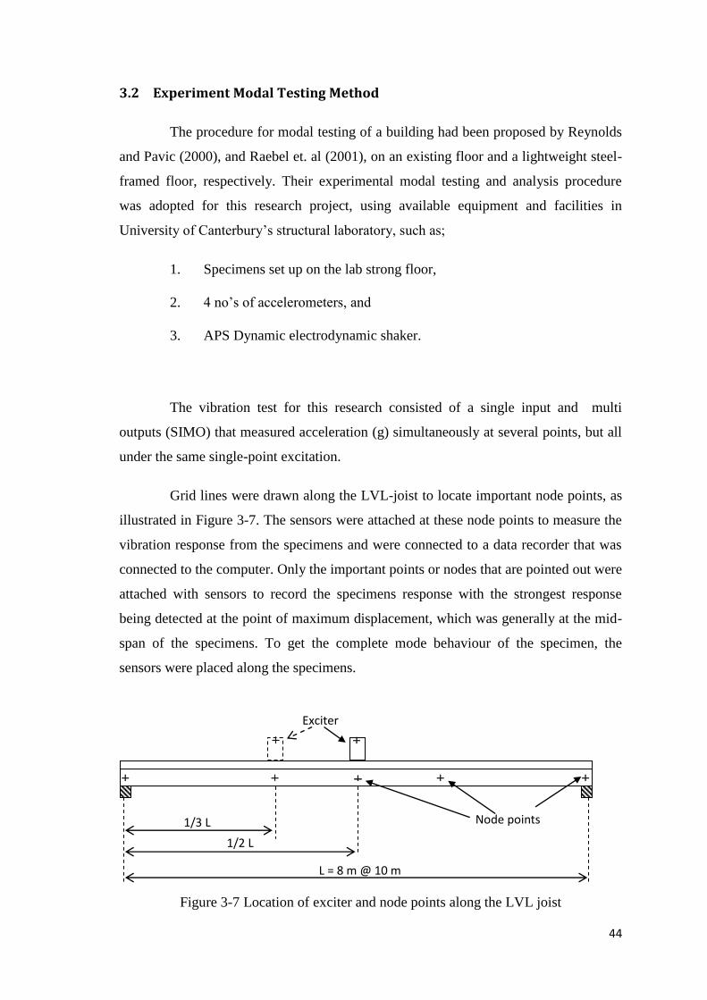
44
3.2 Experiment Modal Testing Method
The procedure for modal testing of a building had been proposed by Reynolds
and Pavic (2000), and Raebel et. al (2001), on an existing floor and a lightweight steel-
framed floor, respectively. Their experimental modal testing and analysis procedure
was adopted for this research project, using available equipment and facilities in
University of Canterbury’s structural laboratory, such as;
1. Specimens set up on the lab strong floor,
2. 4 no’s of accelerometers, and
3. APS Dynamic electrodynamic shaker.
The vibration test for this research consisted of a single input and multi
outputs (SIMO) that measured acceleration (g) simultaneously at several points, but all
under the same single-point excitation.
Grid lines were drawn along the LVL-joist to locate important node points, as
illustrated in Figure 3-7. The sensors were attached at these node points to measure the
vibration response from the specimens and were connected to a data recorder that was
connected to the computer. Only the important points or nodes that are pointed out were
attached with sensors to record the specimens response with the strongest response
being detected at the point of maximum displacement, which was generally at the mid-
span of the specimens. To get the complete mode behaviour of the specimen, the
sensors were placed along the specimens.
Figure 3-7 Location of exciter and node points along the LVL joist
Exciter
L = 8 m @ 10 m
Node points 1/3 L
1/2 L
45
At the beginning, only four (4) roving sensors were available for this research
to measure the vibration response on specimen A. At a later stage, four (4) additional
sensors were supplied for the rest of vibration tests on specimens B, C and D, hence a
total of eight (8) sensors were used. One sensor was placed on the shaker armature to
record the input responses. The place of the sensor should be careful, either at node
points (no displacement) or antinode points (maximum displacement) to get better
mode shapes.
The vertical force excitation was produced by an APS Dynamic
electrodynamic shaker, which was placed on top of the specimens, as illustrated in
Figure 3-7. The shaker was placed at two different locations, (a) at mid-span of the
specimen (1st test) and (b) at one-third length of the specimen (2
nd test). The second
location was to ensure that higher modes (2nd
and 3rd
mode) were also excited, which
were probably missed during the 1st test (shaker at mid-span), as it was suggested by
Reynolds and Pavic (2000) that the location of the exciter should be far away from the
maximum point of deflection or antinodes of any of the important modes.
The shaker excited the specimens with the excitation signals generated by the
signal generator. A stepped sine signal was used to generate the excitation signal for all
vibration tests as it was not possible to use broadband excitation signals in the
structures laboratory. There were two main reasons for performing step sine testing.
Firstly, a step sine excitation signal gives a signal to the shaker/amplifier system with a
finite power output. This is important if there is a requirement to test a structure, which
cannot be excited sufficiently using broadband excitation. Secondly, the sinusoidal
excitation is the best form of excitation for quantifying any non-linearity in a test
structure (Reynolds and Pavic, 2000).
In this research, the signal frequency applied went from 0 Hz up to a
maximum to find the maximum amplitude of the specimen, known as a pre-test. The
range of the input frequency applied to the exciter was then decided based on the pre-
test results and changed depending on the specimen stiffness and the cross section.
Then, the frequencies selected were based on the resonance of the specimen. If the
specimen had a resonance at input frequency of 10 Hz, then the frequency applied was
from 1 Hz to 20 Hz, in 0.1 Hz increments. This was done in order to plot the graph to
determine the natural frequency and critical damping ratio for the specimens.
46
3.3 Modal Parameter Extraction Method
The experimental modal parameters were estimated by a curve-fitting routine
that was available in the ME'scope (ME'scope,2008) data processing software package.
Initially, the single sinusoidal responses were combined manually using MATLAB to
acquire the complete sinusoidal responses from a low frequency (i.e. 5 Hz) to a high
frequency (i.e. 23 Hz). Before the test was conducted, a few trial and error
measurements were performed to determine the optimum data acquisition parameters,
as illustrated in Table 3-2, where the fundamental relationships are follows ;
i. Time window length (s), T = RL / 2.56 (BW)
ii. Sample rate (Hz), SR = RL/T
= 2.56 (BW)
iii. Frequency resolution, FR = 1 / T
= BW / 2.56
where;
BW = usable frequency bandwith (Hz);
RL = record length using the number of the discrete points in
the time history, often a fixed quantity on an FFT based
analyzer;
FR = frequency resolution which is the frequency step between data
points
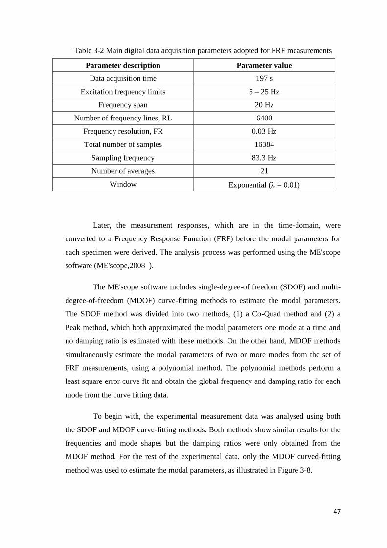
47
Table 3-2 Main digital data acquisition parameters adopted for FRF measurements
Parameter description Parameter value
Data acquisition time 197 s
Excitation frequency limits 5 – 25 Hz
Frequency span 20 Hz
Number of frequency lines, RL 6400
Frequency resolution, FR 0.03 Hz
Total number of samples 16384
Sampling frequency 83.3 Hz
Number of averages 21
Window Exponential ( = 0.01)
Later, the measurement responses, which are in the time-domain, were
converted to a Frequency Response Function (FRF) before the modal parameters for
each specimen were derived. The analysis process was performed using the ME'scope
software (ME'scope,2008 ).
The ME'scope software includes single-degree-of freedom (SDOF) and multi-
degree-of-freedom (MDOF) curve-fitting methods to estimate the modal parameters.
The SDOF method was divided into two methods, (1) a Co-Quad method and (2) a
Peak method, which both approximated the modal parameters one mode at a time and
no damping ratio is estimated with these methods. On the other hand, MDOF methods
simultaneously estimate the modal parameters of two or more modes from the set of
FRF measurements, using a polynomial method. The polynomial methods perform a
least square error curve fit and obtain the global frequency and damping ratio for each
mode from the curve fitting data.
To begin with, the experimental measurement data was analysed using both
the SDOF and MDOF curve-fitting methods. Both methods show similar results for the
frequencies and mode shapes but the damping ratios were only obtained from the
MDOF method. For the rest of the experimental data, only the MDOF curved-fitting
method was used to estimate the modal parameters, as illustrated in Figure 3-8.
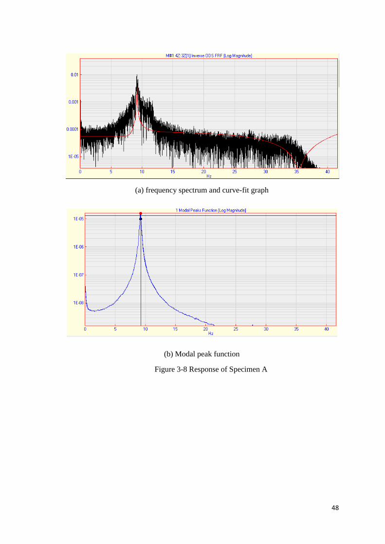
48
(a) frequency spectrum and curve-fit graph
(b) Modal peak function
Figure 3-8 Response of Specimen A
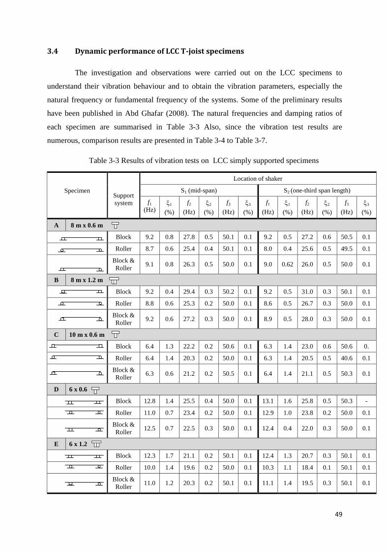
49
3.4 Dynamic performance of LCC T-joist specimens
The investigation and observations were carried out on the LCC specimens to
understand their vibration behaviour and to obtain the vibration parameters, especially the
natural frequency or fundamental frequency of the systems. Some of the preliminary results
have been published in Abd Ghafar (2008). The natural frequencies and damping ratios of
each specimen are summarised in Table 3-3 Also, since the vibration test results are
numerous, comparison results are presented in Table 3-4 to Table 3-7.
Table 3-3 Results of vibration tests on LCC simply supported specimens
Specimen
S
Support
system
Location of shaker
S1 (mid-span) S2 (one-third span length)
f1
(Hz) 1
(%)
f2
(Hz)
2
(%)
f3
(Hz)
3
(%)
f1
(Hz)
1
(%)
f2
(Hz)
2
(%)
f3
(Hz)
3
(%)
A 8 m x 0.6 m
Block 9.2 0.8 27.8 0.5 50.1 0.1 9.2 0.5 27.2 0.6 50.5 0.1
Roller 8.7 0.6 25.4 0.4 50.1 0.1 8.0 0.4 25.6 0.5 49.5 0.1
Block &
Roller 9.1 0.8 26.3 0.5 50.0 0.1 9.0 0.62 26.0 0.5 50.0 0.1
B 8 m x 1.2 m
Block 9.2 0.4 29.4 0.3 50.2 0.1 9.2 0.5 31.0 0.3 50.1 0.1
Roller 8.8 0.6 25.3 0.2 50.0 0.1 8.6 0.5 26.7 0.3 50.0 0.1
Block &
Roller 9.2 0.6 27.2 0.3 50.0 0.1 8.9 0.5 28.0 0.3 50.0 0.1
C 10 m x 0.6 m
Block 6.4 1.3 22.2 0.2 50.6 0.1 6.3 1.4 23.0 0.6 50.6 0.
Roller 6.4 1.4 20.3 0.2 50.0 0.1 6.3 1.4 20.5 0.5 40.6 0.1
Block &
Roller 6.3 0.6 21.2 0.2 50.5 0.1 6.4 1.4 21.1 0.5 50.3 0.1
D 6 x 0.6
Block 12.8 1.4 25.5 0.4 50.0 0.1 13.1 1.6 25.8 0.5 50.3 -
Roller 11.0 0.7 23.4 0.2 50.0 0.1 12.9 1.0 23.8 0.2 50.0 0.1
Block &
Roller 12.5 0.7 22.5 0.3 50.0 0.1 12.4 0.4 22.0 0.3 50.0 0.1
E 6 x 1.2
Block 12.3 1.7 21.1 0.2 50.1 0.1 12.4 1.3 20.7 0.3 50.1 0.1
Roller 10.0 1.4 19.6 0.2 50.0 0.1 10.3 1.1 18.4 0.1 50.1 0.1
Block &
Roller 11.0 1.2 20.3 0.2 50.1 0.1 11.1 1.4 19.5 0.3 50.1 0.1
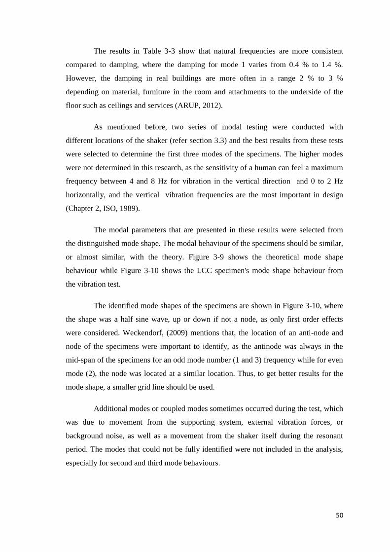
50
The results in Table 3-3 show that natural frequencies are more consistent
compared to damping, where the damping for mode 1 varies from 0.4 % to 1.4 %.
However, the damping in real buildings are more often in a range 2 % to 3 %
depending on material, furniture in the room and attachments to the underside of the
floor such as ceilings and services (ARUP, 2012).
As mentioned before, two series of modal testing were conducted with
different locations of the shaker (refer section 3.3) and the best results from these tests
were selected to determine the first three modes of the specimens. The higher modes
were not determined in this research, as the sensitivity of a human can feel a maximum
frequency between 4 and 8 Hz for vibration in the vertical direction and 0 to 2 Hz
horizontally, and the vertical vibration frequencies are the most important in design
(Chapter 2, ISO, 1989).
The modal parameters that are presented in these results were selected from
the distinguished mode shape. The modal behaviour of the specimens should be similar,
or almost similar, with the theory. Figure 3-9 shows the theoretical mode shape
behaviour while Figure 3-10 shows the LCC specimen's mode shape behaviour from
the vibration test.
The identified mode shapes of the specimens are shown in Figure 3-10, where
the shape was a half sine wave, up or down if not a node, as only first order effects
were considered. Weckendorf, (2009) mentions that, the location of an anti-node and
node of the specimens were important to identify, as the antinode was always in the
mid-span of the specimens for an odd mode number (1 and 3) frequency while for even
mode (2), the node was located at a similar location. Thus, to get better results for the
mode shape, a smaller grid line should be used.
Additional modes or coupled modes sometimes occurred during the test, which
was due to movement from the supporting system, external vibration forces, or
background noise, as well as a movement from the shaker itself during the resonant
period. The modes that could not be fully identified were not included in the analysis,
especially for second and third mode behaviours.
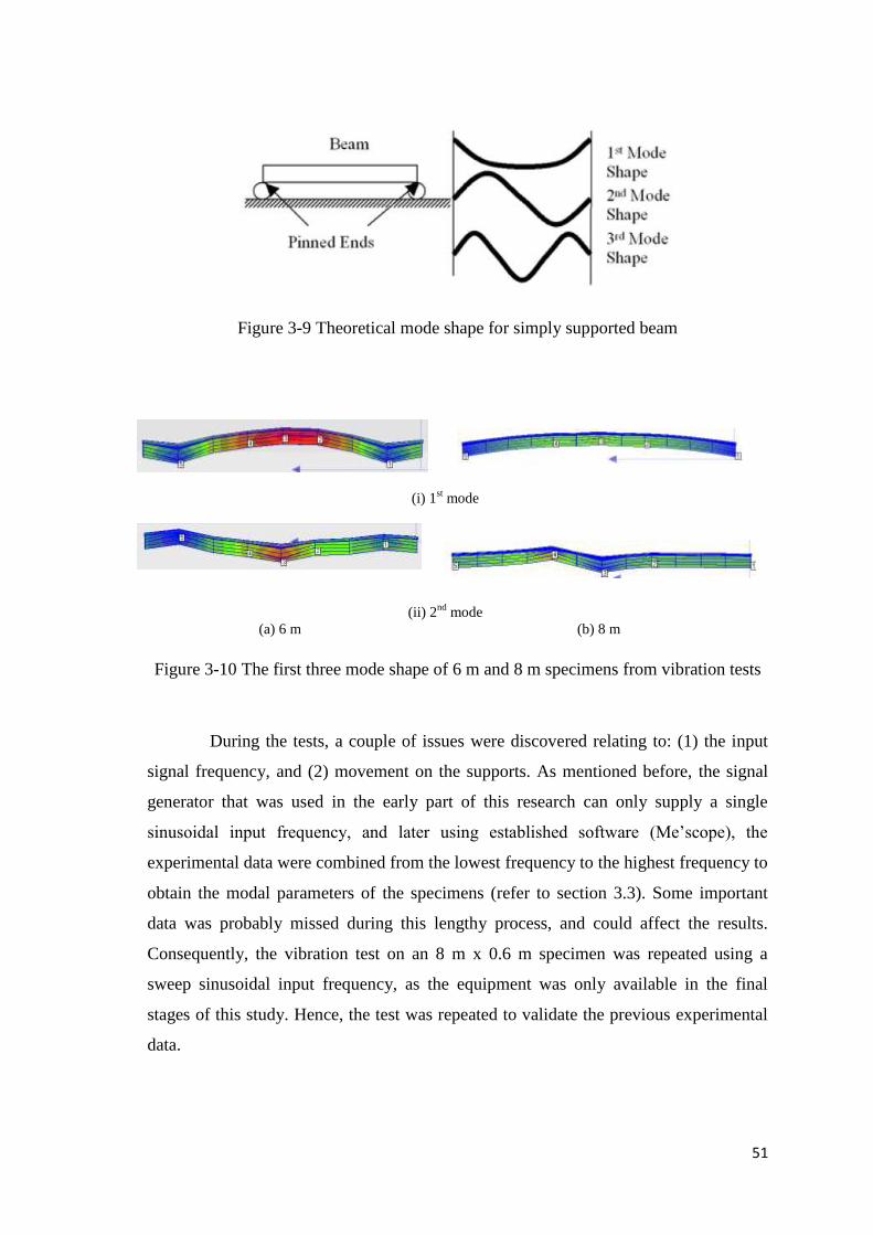
51
Figure 3-9 Theoretical mode shape for simply supported beam
(i) 1st mode
(ii) 2nd
mode
(a) 6 m (b) 8 m
Figure 3-10 The first three mode shape of 6 m and 8 m specimens from vibration tests
During the tests, a couple of issues were discovered relating to: (1) the input
signal frequency, and (2) movement on the supports. As mentioned before, the signal
generator that was used in the early part of this research can only supply a single
sinusoidal input frequency, and later using established software (Me’scope), the
experimental data were combined from the lowest frequency to the highest frequency to
obtain the modal parameters of the specimens (refer to section 3.3). Some important
data was probably missed during this lengthy process, and could affect the results.
Consequently, the vibration test on an 8 m x 0.6 m specimen was repeated using a
sweep sinusoidal input frequency, as the equipment was only available in the final
stages of this study. Hence, the test was repeated to validate the previous experimental
data.
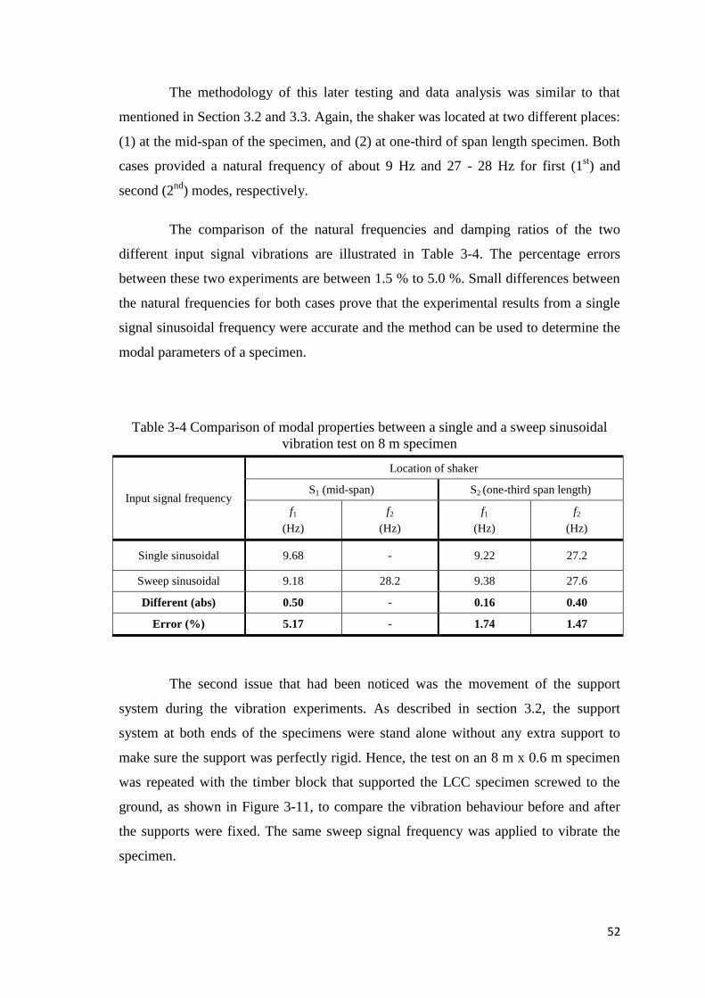
52
The methodology of this later testing and data analysis was similar to that
mentioned in Section 3.2 and 3.3. Again, the shaker was located at two different places:
(1) at the mid-span of the specimen, and (2) at one-third of span length specimen. Both
cases provided a natural frequency of about 9 Hz and 27 - 28 Hz for first (1st) and
second (2nd
) modes, respectively.
The comparison of the natural frequencies and damping ratios of the two
different input signal vibrations are illustrated in Table 3-4. The percentage errors
between these two experiments are between 1.5 % to 5.0 %. Small differences between
the natural frequencies for both cases prove that the experimental results from a single
signal sinusoidal frequency were accurate and the method can be used to determine the
modal parameters of a specimen.
Table 3-4 Comparison of modal properties between a single and a sweep sinusoidal
vibration test on 8 m specimen
Input signal frequency
Location of shaker
S1 (mid-span) S2 (one-third span length)
f1
(Hz)
f2
(Hz)
f1
(Hz)
f2
(Hz)
Single sinusoidal 9.68 - 9.22 27.2
Sweep sinusoidal 9.18 28.2 9.38 27.6
Different (abs) 0.50 - 0.16 0.40
Error (%) 5.17 - 1.74 1.47
The second issue that had been noticed was the movement of the support
system during the vibration experiments. As described in section 3.2, the support
system at both ends of the specimens were stand alone without any extra support to
make sure the support was perfectly rigid. Hence, the test on an 8 m x 0.6 m specimen
was repeated with the timber block that supported the LCC specimen screwed to the
ground, as shown in Figure 3-11, to compare the vibration behaviour before and after
the supports were fixed. The same sweep signal frequency was applied to vibrate the
specimen.
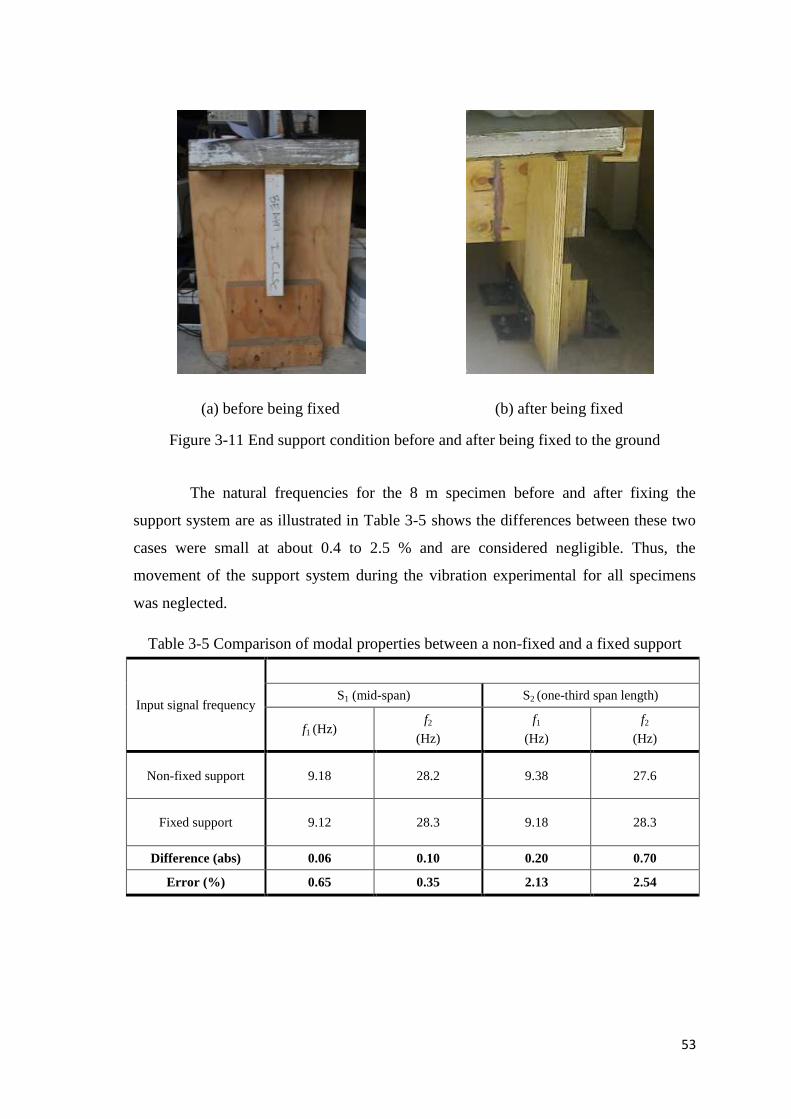
53
(a) before being fixed
(b) after being fixed
Figure 3-11 End support condition before and after being fixed to the ground
The natural frequencies for the 8 m specimen before and after fixing the
support system are as illustrated in Table 3-5 shows the differences between these two
cases were small at about 0.4 to 2.5 % and are considered negligible. Thus, the
movement of the support system during the vibration experimental for all specimens
was neglected.
Table 3-5 Comparison of modal properties between a non-fixed and a fixed support
Input signal frequency
S1 (mid-span) S2 (one-third span length)
f1 (Hz) f2
(Hz)
f1
(Hz)
f2
(Hz)
Non-fixed support 9.18 28.2 9.38 27.6
Fixed support 9.12 28.3 9.18 28.3
Difference (abs) 0.06 0.10 0.20 0.70
Error (%) 0.65 0.35 2.13 2.54
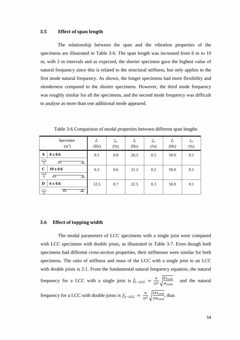
54
3.5 Effect of span length
The relationship between the span and the vibration properties of the
specimens are illustrated in Table 3-6. The span length was increased from 6 m to 10
m, with 2 m intervals and as expected, the shorter specimen gave the highest value of
natural frequency since this is related to the structural stiffness, but only applies to the
first mode natural frequency. As shown, the longer specimens had more flexibility and
slenderness compared to the shorter specimens. However, the third mode frequency
was roughly similar for all the specimens, and the second mode frequency was difficult
to analyse as more than one additional mode appeared.
Table 3-6 Comparison of modal properties between different span lengths
Specimen
(m2)
f1
(Hz)
1
(%)
f2
(Hz)
3
(%)
f3
(Hz)
3
(%)
A 8 x 0.6 9.1
0.8
26.3
0.5
50.0
0.1
C 10 x 0.6 6.3
0.6
21.2
0.2
50.0
0.1
D 6 x 0.6 12.5
0.7
22.5
0.3
50.0
0.1
3.6 Effect of topping width
The modal parameters of LCC specimens with a single joist were compared
with LCC specimens with double joists, as illustrated in Table 3-7. Even though both
specimens had different cross-section properties, their stiffnesses were similar for both
specimens. The ratio of stiffness and mass of the LCC with a single joist to an LCC
with double joists is 2:1. From the fundamental natural frequency equation, the natural
frequency for a LCC with a single joist is
and the natural
frequency for a LCC with double joists is
, thus
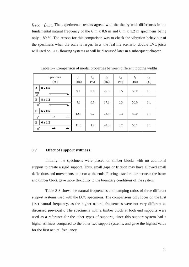
55
f1-LCC = f2-LCC. The experimental results agreed with the theory with differences in the
fundamental natural frequency of the 6 m x 0.6 m and 6 m x 1.2 m specimens being
only 1.80 %. The reason for this comparison was to check the vibration behaviour of
the specimens when the scale is larger. In a the real life scenario, double LVL joists
will used on LCC flooring systems as will be discussed later in a subsequent chapter.
Table 3-7 Comparison of modal properties between different topping widths
Specimen
(m2)
f1
(Hz)
1
(%)
f2
(Hz)
2
(%)
f3
(Hz)
3
(%)
A 8 x 0.6 9.1 0.8 26.3 0.5 50.0 0.1
B 8 x 1.2 9.2 0.6 27.2 0.3 50.0 0.1
D 6 x 0.6 12.5 0.7 22.5 0.3 50.0 0.1
E 6 x 1.2 11.0 1.2 20.3 0.2 50.1 0.1
3.7 Effect of support stiffness
Initially, the specimens were placed on timber blocks with no additional
support to create a rigid support. Thus, small gaps or friction may have allowed small
deflections and movements to occur at the ends. Placing a steel roller between the beam
and timber block gave more flexibility to the boundary conditions of the system.
Table 3-8 shows the natural frequencies and damping ratios of three different
support systems used with the LCC specimens. The comparisons only focus on the first
(1st) natural frequency, as the higher natural frequencies were not very different as
discussed previously. The specimens with a timber block at both end supports were
used as a reference for the other types of supports, since this support system had a
higher stiffness compared to the other two support systems, and gave the highest value
for the first natural frequency.
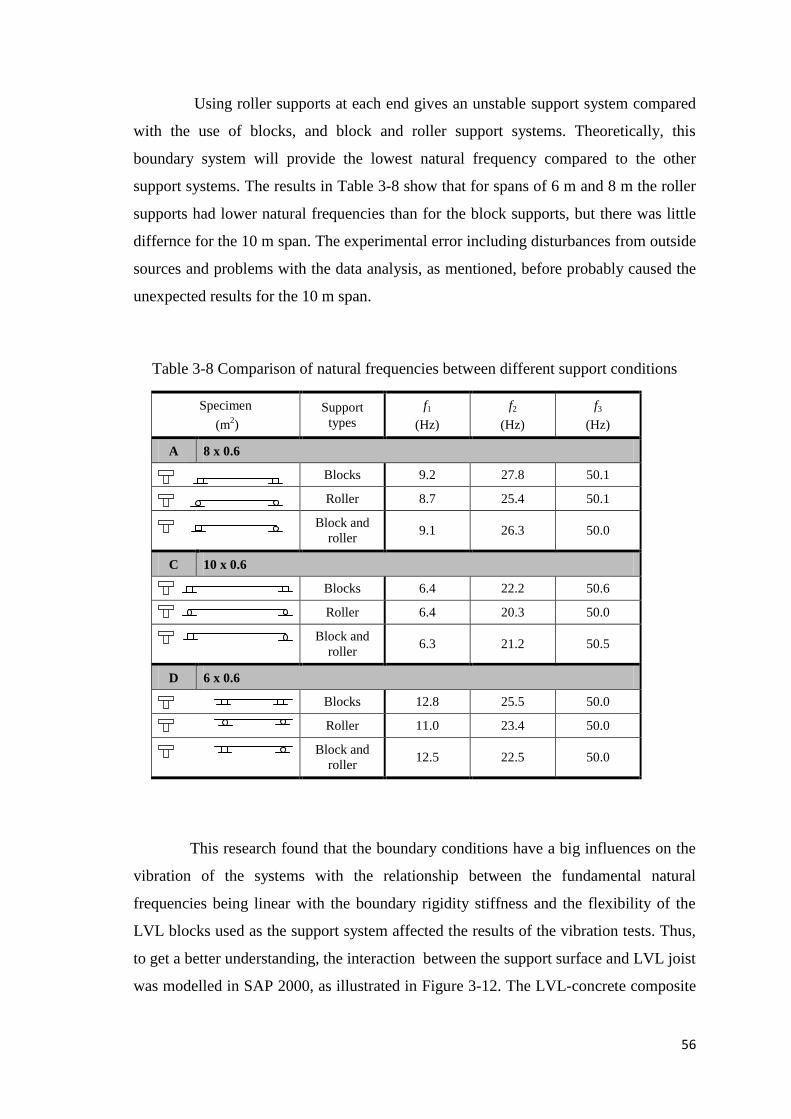
56
Using roller supports at each end gives an unstable support system compared
with the use of blocks, and block and roller support systems. Theoretically, this
boundary system will provide the lowest natural frequency compared to the other
support systems. The results in Table 3-8 show that for spans of 6 m and 8 m the roller
supports had lower natural frequencies than for the block supports, but there was little
differnce for the 10 m span. The experimental error including disturbances from outside
sources and problems with the data analysis, as mentioned, before probably caused the
unexpected results for the 10 m span.
Table 3-8 Comparison of natural frequencies between different support conditions
Specimen
(m2)
Support
types
f1
(Hz)
f2
(Hz)
f3
(Hz)
A 8 x 0.6
Blocks 9.2 27.8 50.1
Roller 8.7 25.4 50.1
Block and
roller 9.1 26.3 50.0
C 10 x 0.6
Blocks 6.4 22.2 50.6
Roller 6.4 20.3 50.0
Block and
roller 6.3 21.2 50.5
D 6 x 0.6
Blocks 12.8 25.5 50.0
Roller 11.0 23.4 50.0
Block and
roller 12.5 22.5 50.0
This research found that the boundary conditions have a big influences on the
vibration of the systems with the relationship between the fundamental natural
frequencies being linear with the boundary rigidity stiffness and the flexibility of the
LVL blocks used as the support system affected the results of the vibration tests. Thus,
to get a better understanding, the interaction between the support surface and LVL joist
was modelled in SAP 2000, as illustrated in Figure 3-12. The LVL-concrete composite
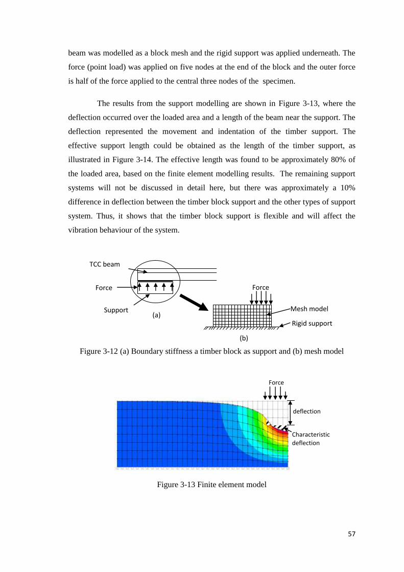
57
beam was modelled as a block mesh and the rigid support was applied underneath. The
force (point load) was applied on five nodes at the end of the block and the outer force
is half of the force applied to the central three nodes of the specimen.
The results from the support modelling are shown in Figure 3-13, where the
deflection occurred over the loaded area and a length of the beam near the support. The
deflection represented the movement and indentation of the timber support. The
effective support length could be obtained as the length of the timber support, as
illustrated in Figure 3-14. The effective length was found to be approximately 80% of
the loaded area, based on the finite element modelling results. The remaining support
systems will not be discussed in detail here, but there was approximately a 10%
difference in deflection between the timber block support and the other types of support
system. Thus, it shows that the timber block support is flexible and will affect the
vibration behaviour of the system.
Figure 3-12 (a) Boundary stiffness a timber block as support and (b) mesh model
Figure 3-13 Finite element model
TCC beam
Support
Force
Force
Mesh model
Rigid support
(a)
(b)
deflection
Force
Characteristic deflection

58
3.8 Finite Element Modelling of LCC T-joist specimens
Finite element analysis (FEA) has become commonly used as a tool to solve
complicated stress problems using a system of points called nodes which make a grid
called a mesh. Material and structural properties were assigned to the elements of the
mesh, such as beam or shell elements to define how the structure will react to certain
loading conditions.
The finite element package, SAP 2000 v.14 (SAP2000, 1997) was used to
model the LCC beams to evaluate the experimental modal analysis results using the
same material properties and cross-section, with a modulus of elasticity for concrete of
Ec = 30 MPa and for timber, Et = 12.7 MPa. The same procedure as described in section
3.2 was applied in this analysis. Additionally, all elements were assumed to have
isotropic material characteristics, including LVL, even though LVL is an orthotropic
material, to get the optimum dynamic behaviour of the system. The complete properties
of concrete and LVL are reported in Appendix A.
The lumped mass system illustrated in Figure 3-15 was modelled in a
preliminary study to find the dynamic behaviour of the TCC beam using the same
configuration as discussed in section 3.2. A more refined finite element (FE) mesh is
outlined in Figure 3-16. Nodes, corresponding to the lumped masses were modelled at
200 mm centres. The connectors were modelled as spring elements with stiffness, k, as
provided by Yeoh (2010). The spring elements were connected between the nodes of
the two elements, while beam elements represented the LVL joist, and shell elements
represented the concrete topping as illustrated in Figure 3-16. The serviceability slip
Effective length
deflection
Fully stressed (uniform)
unstressed
Figure 3-14 Support effective width
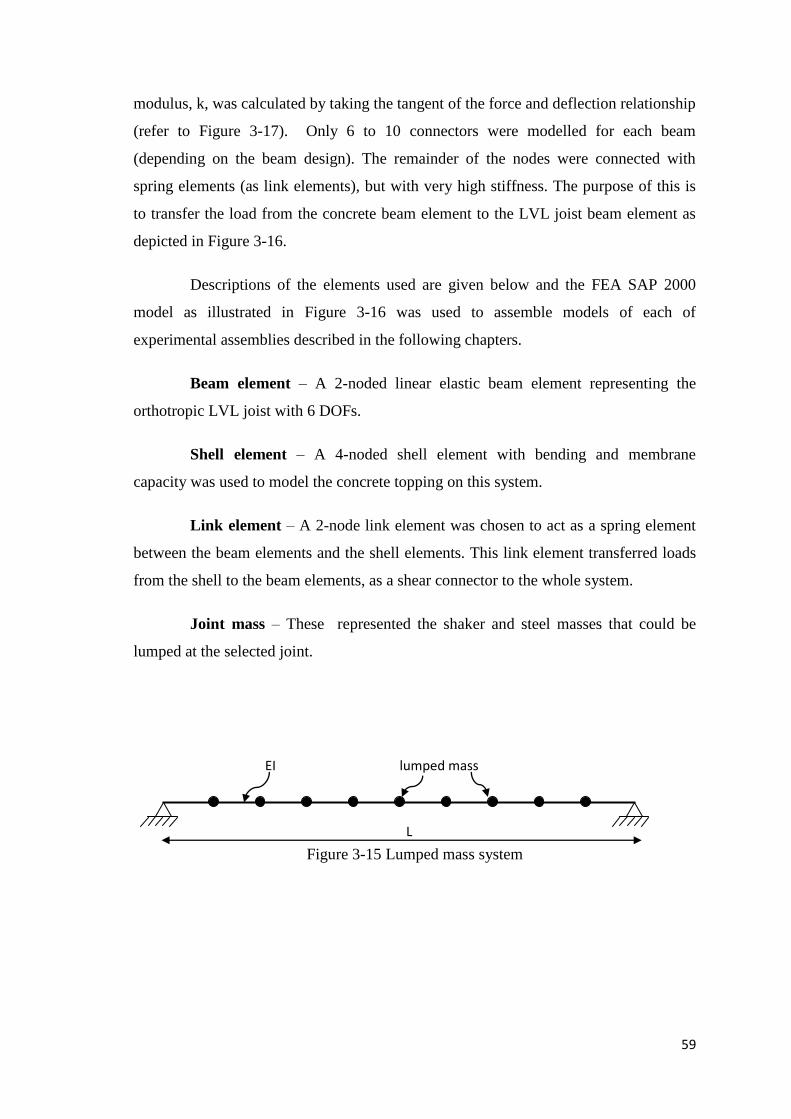
59
modulus, k, was calculated by taking the tangent of the force and deflection relationship
(refer to Figure 3-17). Only 6 to 10 connectors were modelled for each beam
(depending on the beam design). The remainder of the nodes were connected with
spring elements (as link elements), but with very high stiffness. The purpose of this is
to transfer the load from the concrete beam element to the LVL joist beam element as
depicted in Figure 3-16.
Descriptions of the elements used are given below and the FEA SAP 2000
model as illustrated in Figure 3-16 was used to assemble models of each of
experimental assemblies described in the following chapters.
Beam element – A 2-noded linear elastic beam element representing the
orthotropic LVL joist with 6 DOFs.
Shell element – A 4-noded shell element with bending and membrane
capacity was used to model the concrete topping on this system.
Link element – A 2-node link element was chosen to act as a spring element
between the beam elements and the shell elements. This link element transferred loads
from the shell to the beam elements, as a shear connector to the whole system.
Joint mass – These represented the shaker and steel masses that could be
lumped at the selected joint.
Figure 3-15 Lumped mass system
lumped mass
L
EI
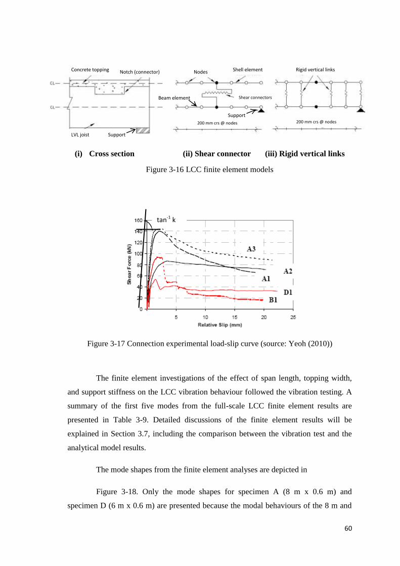
60
(i) Cross section (ii) Shear connector (iii) Rigid vertical links
Figure 3-16 LCC finite element models
Figure 3-17 Connection experimental load-slip curve (source: Yeoh (2010))
The finite element investigations of the effect of span length, topping width,
and support stiffness on the LCC vibration behaviour followed the vibration testing. A
summary of the first five modes from the full-scale LCC finite element results are
presented in Table 3-9. Detailed discussions of the finite element results will be
explained in Section 3.7, including the comparison between the vibration test and the
analytical model results.
The mode shapes from the finite element analyses are depicted in
Figure 3-18. Only the mode shapes for specimen A (8 m x 0.6 m) and
specimen D (6 m x 0.6 m) are presented because the modal behaviours of the 8 m and
tan-1 k
Nodes Notch (connector)
LVL joist Support
Concrete topping Shell element
200 mm crs @ nodes
Rigid vertical links
Beam element Shear connectors
Support 200 mm crs @ nodes
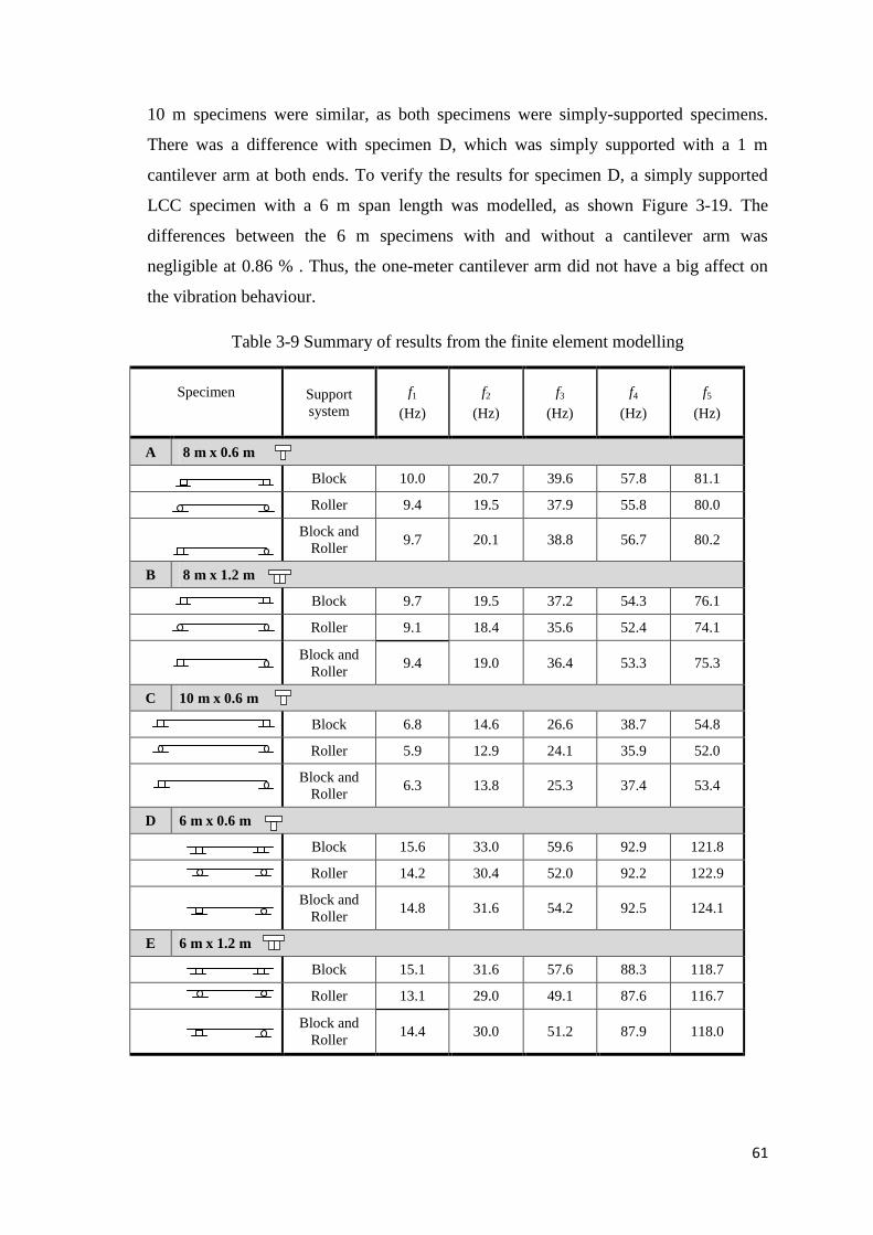
61
10 m specimens were similar, as both specimens were simply-supported specimens.
There was a difference with specimen D, which was simply supported with a 1 m
cantilever arm at both ends. To verify the results for specimen D, a simply supported
LCC specimen with a 6 m span length was modelled, as shown Figure 3-19. The
differences between the 6 m specimens with and without a cantilever arm was
negligible at 0.86 % . Thus, the one-meter cantilever arm did not have a big affect on
the vibration behaviour.
Table 3-9 Summary of results from the finite element modelling
Specimen
Support
system
f1
(Hz)
f2
(Hz)
f3
(Hz)
f4
(Hz)
f5
(Hz)
A 8 m x 0.6 m
Block 10.0 20.7 39.6 57.8 81.1
Roller 9.4 19.5 37.9 55.8 80.0
Block and
Roller 9.7 20.1 38.8 56.7 80.2
B 8 m x 1.2 m
Block 9.7 19.5 37.2 54.3 76.1
Roller 9.1 18.4 35.6 52.4 74.1
Block and
Roller 9.4 19.0 36.4 53.3 75.3
C 10 m x 0.6 m
Block 6.8 14.6 26.6 38.7 54.8
Roller 5.9 12.9 24.1 35.9 52.0
Block and
Roller 6.3 13.8 25.3 37.4 53.4
D 6 m x 0.6 m
Block 15.6 33.0 59.6 92.9 121.8
Roller 14.2 30.4 52.0 92.2 122.9
Block and
Roller 14.8 31.6 54.2 92.5 124.1
E 6 m x 1.2 m
Block 15.1 31.6 57.6 88.3 118.7
Roller 13.1 29.0 49.1 87.6 116.7
Block and
Roller 14.4 30.0 51.2 87.9 118.0
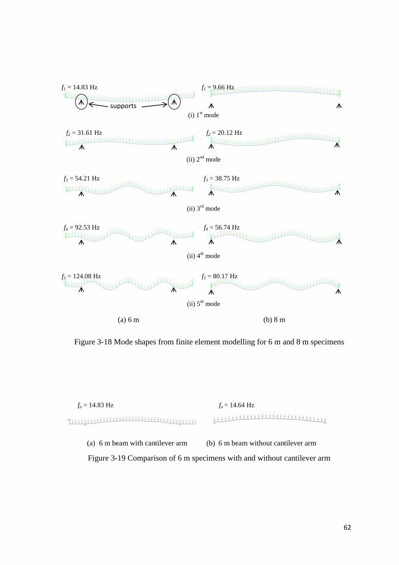
62
(i) 1st mode
(ii) 2nd
mode
(ii) 3rd
mode
(ii) 4th
mode
(ii) 5th
mode
(a) 6 m (b) 8 m
Figure 3-18 Mode shapes from finite element modelling for 6 m and 8 m specimens
(a) 6 m beam with cantilever arm (b) 6 m beam without cantilever arm
Figure 3-19 Comparison of 6 m specimens with and without cantilever arm
supports
fn = 14.83 Hz
fn = 14.64 Hz
f1 = 14.83 Hz
f2 = 31.61 Hz
f3 = 54.21 Hz
f4 = 92.53 Hz
f5 = 124.08 Hz
f1 = 9.66 Hz
f2 = 20.12 Hz
f3 = 38.75 Hz
f4 = 56.74 Hz
f5 = 80.17 Hz
63
3.9 Comparison between the modal test (EMA) and finite element
modelling (FEA)
The discussion of the comparison between the EMA and FEA only focuses on
the fundamental frequency, since some of the higher modes from the EMA could not be
obtained for some specimens. In addition, the fundamental natural frequency is the
most important frequency for serviceability in a structural design compared to the
higher frequencies.
Table 3-10 shows the differences in fundamental natural frequency between
analytical modelling and vibration test results, together with the percentage errors,
based on the support systems of the specimens. The differences in the fundamental
natural frequencies predicted from the FEA and EMA was moderately high with the
average errors for specimens on blocks, rollers, and block and roller support systems
being about 11.5 %, 13.0 % and 9.5 %, or 1.8 Hz, 1.1 Hz or 0.8 Hz, respectively. The
flexibility of the support systems in the tests probably caused the big differences. As
discussed before (see section 3.2), the specimens were placed on a LVL block which
acted as the support system. The flexibility of the LVL block may have affected the
overall vibration behaviour of the specimens. Meanwhile, the support systems in FEA
modelling were more rigid than the real situation.
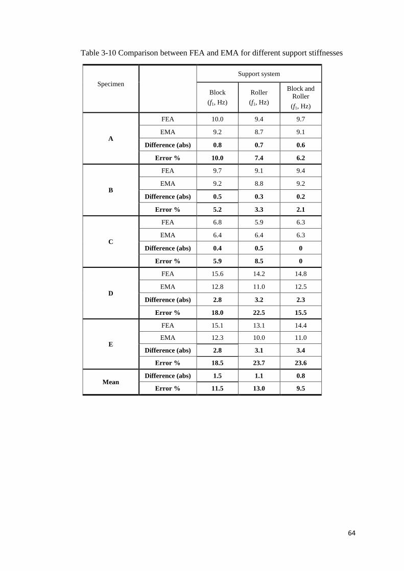
64
Table 3-10 Comparison between FEA and EMA for different support stiffnesses
Specimen
Support system
Block
(f1, Hz)
Roller
(f1, Hz)
Block and
Roller
(f1, Hz)
A
FEA 10.0 9.4 9.7
EMA 9.2 8.7 9.1
Difference (abs) 0.8 0.7 0.6
Error % 10.0 7.4 6.2
B
FEA 9.7 9.1 9.4
EMA 9.2 8.8 9.2
Difference (abs) 0.5 0.3 0.2
Error % 5.2 3.3 2.1
C
FEA 6.8 5.9 6.3
EMA 6.4 6.4 6.3
Difference (abs) 0.4 0.5 0
Error % 5.9 8.5 0
D
FEA 15.6 14.2 14.8
EMA 12.8 11.0 12.5
Difference (abs) 2.8 3.2 2.3
Error % 18.0 22.5 15.5
E
FEA 15.1 13.1 14.4
EMA 12.3 10.0 11.0
Difference (abs) 2.8 3.1 3.4
Error % 18.5 23.7 23.6
Mean Difference (abs) 1.5 1.1 0.8
Error % 11.5 13.0 9.5
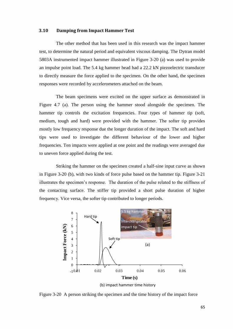
65
3.10 Damping from Impact Hammer Test
The other method that has been used in this research was the impact hammer
test, to determine the natural period and equivalent viscous damping. The Dytran model
5803A instrumented impact hammer illustrated in Figure 3-20 (a) was used to provide
an impulse point load. The 5.4 kg hammer head had a 22.2 kN piezoelectric transducer
to directly measure the force applied to the specimen. On the other hand, the specimen
responses were recorded by accelerometers attached on the beam.
The beam specimens were excited on the upper surface as demonstrated in
Figure 4.7 (a). The person using the hammer stood alongside the specimen. The
hammer tip controls the excitation frequencies. Four types of hammer tip (soft,
medium, tough and hard) were provided with the hammer. The softer tip provides
mostly low frequency response due the longer duration of the impact. The soft and hard
tips were used to investigate the different behaviour of the lower and higher
frequencies. Ten impacts were applied at one point and the readings were averaged due
to uneven force applied during the test.
Striking the hammer on the specimen created a half-sine input curve as shown
in Figure 3-20 (b), with two kinds of force pulse based on the hammer tip. Figure 3-21
illustrates the specimen’s response. The duration of the pulse related to the stiffness of
the contacting surface. The stiffer tip provided a short pulse duration of higher
frequency. Vice versa, the softer tip contributed to longer periods.
Figure 3-20 A person striking the specimen and the time history of the impact force
-1
0
1
2
3
4
5
6
7
8
0.01 0.02 0.03 0.04 0.05 0.06
Imp
act
Forc
e (k
N)
Time (s)
Hard tip
Soft tip
(a)
(b) impact hammer time history
Interchangeable
impact tip
5.5 kg hammer
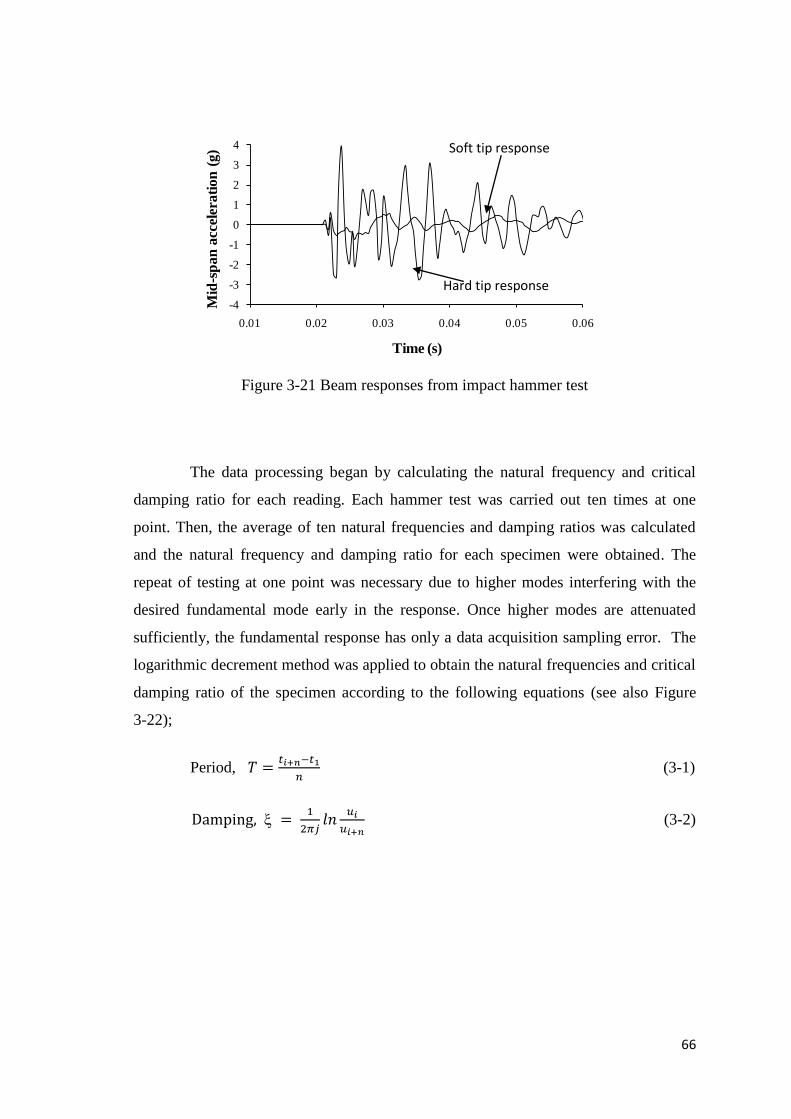
66
Figure 3-21 Beam responses from impact hammer test
The data processing began by calculating the natural frequency and critical
damping ratio for each reading. Each hammer test was carried out ten times at one
point. Then, the average of ten natural frequencies and damping ratios was calculated
and the natural frequency and damping ratio for each specimen were obtained. The
repeat of testing at one point was necessary due to higher modes interfering with the
desired fundamental mode early in the response. Once higher modes are attenuated
sufficiently, the fundamental response has only a data acquisition sampling error. The
logarithmic decrement method was applied to obtain the natural frequencies and critical
damping ratio of the specimen according to the following equations (see also Figure
3-22);
Period,
(3-1)
(3-2)
-4
-3
-2
-1
0
1
2
3
4
0.01 0.02 0.03 0.04 0.05 0.06
Mid
-sp
an
acc
eler
ati
on
(g
)
Time (s)
Soft tip response
Hard tip response
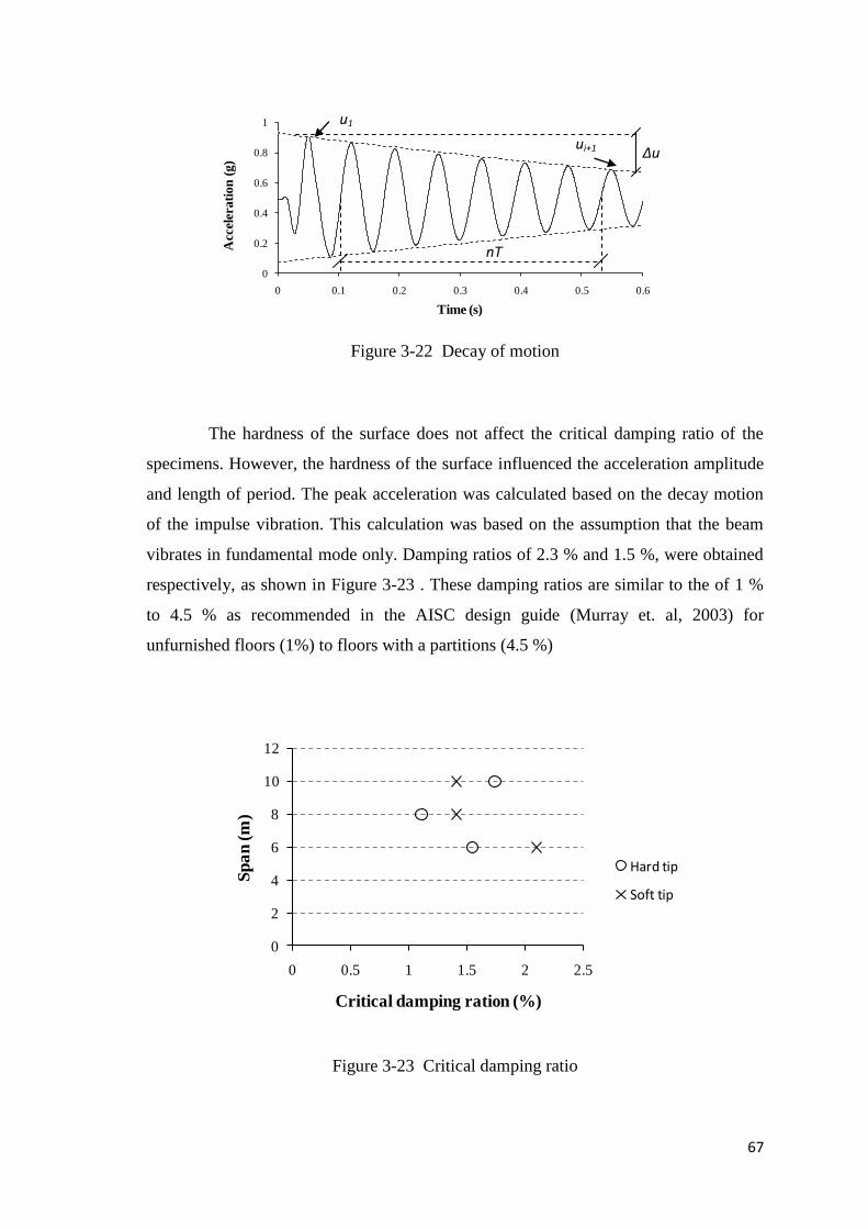
67
Figure 3-22 Decay of motion
The hardness of the surface does not affect the critical damping ratio of the
specimens. However, the hardness of the surface influenced the acceleration amplitude
and length of period. The peak acceleration was calculated based on the decay motion
of the impulse vibration. This calculation was based on the assumption that the beam
vibrates in fundamental mode only. Damping ratios of 2.3 % and 1.5 %, were obtained
respectively, as shown in Figure 3-23 . These damping ratios are similar to the of 1 %
to 4.5 % as recommended in the AISC design guide (Murray et. al, 2003) for
unfurnished floors (1%) to floors with a partitions (4.5 %)
Figure 3-23 Critical damping ratio
0
0.2
0.4
0.6
0.8
1
0 0.1 0.2 0.3 0.4 0.5 0.6
Acc
eler
ati
on
(g)
Time (s)
0
2
4
6
8
10
12
0 5 10 15 20
Sp
an
(m
)
Natural Frequency (Hz)
Hard tip
Soft tip
0
2
4
6
8
10
12
0 0.5 1 1.5 2 2.5
Sp
an
(m
)
Critical damping ration (%)
Hard tip
Soft tip
uj+1
u1
nT
Δu
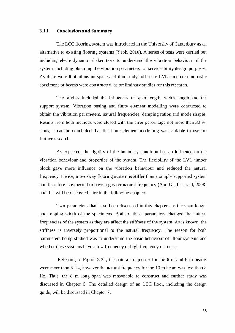
68
3.11 Conclusion and Summary
The LCC flooring system was introduced in the University of Canterbury as an
alternative to existing flooring systems (Yeoh, 2010). A series of tests were carried out
including electrodynamic shaker tests to understand the vibration behaviour of the
system, including obtaining the vibration parameters for serviceability design purposes.
As there were limitations on space and time, only full-scale LVL-concrete composite
specimens or beams were constructed, as preliminary studies for this research.
The studies included the influences of span length, width length and the
support system. Vibration testing and finite element modelling were conducted to
obtain the vibration parameters, natural frequencies, damping ratios and mode shapes.
Results from both methods were closed with the error percentage not more than 30 %.
Thus, it can be concluded that the finite element modelling was suitable to use for
further research.
As expected, the rigidity of the boundary condition has an influence on the
vibration behaviour and properties of the system. The flexibility of the LVL timber
block gave more influence on the vibration behaviour and reduced the natural
frequency. Hence, a two-way flooring system is stiffer than a simply supported system
and therefore is expected to have a greater natural frequency (Abd Ghafar et. al, 2008)
and this will be discussed later in the following chapters.
Two parameters that have been discussed in this chapter are the span length
and topping width of the specimens. Both of these parameters changed the natural
frequencies of the system as they are affect the stiffness of the system. As is known, the
stiffness is inversely proportional to the natural frequency. The reason for both
parameters being studied was to understand the basic behaviour of floor systems and
whether these systems have a low frequency or high frequency response.
Referring to Figure 3-24, the natural frequency for the 6 m and 8 m beams
were more than 8 Hz, however the natural frequency for the 10 m beam was less than 8
Hz. Thus, the 8 m long span was reasonable to construct and further study was
discussed in Chapter 6. The detailed design of an LCC floor, including the design
guide, will be discussed in Chapter 7.
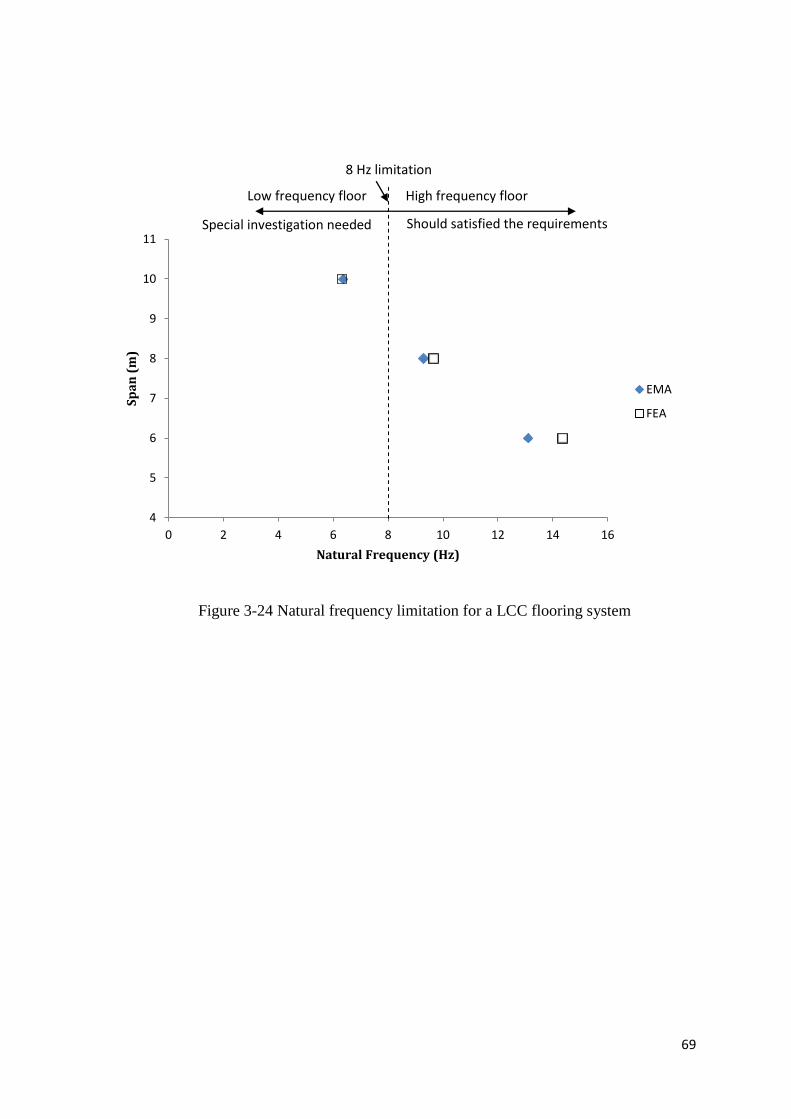
69
Figure 3-24 Natural frequency limitation for a LCC flooring system
4
5
6
7
8
9
10
11
0 2 4 6 8 10 12 14 16
Sp
an
(m
)
Natural Frequency (Hz)
EMA
FEA
Special investigation needed
Should satisfied the requirements
High frequency floor
Low frequency floor
8 Hz limitation
CHAPTER 4 EXPERIMENTAL MODAL ANALYSIS (EMA) ON
REDUCED SCALE LVL-CONCRETE COMPOSITE (LCC)
T-JOIST SPECIMENS
In this chapter, details of Experimental Modal Analysis (EMA) and Finite
Element (FE) modelling of reduced-scale LCC T-joist specimens and floor are
presented. The details were implemented from the full-scale LCC specimens discussed
in Chapter 3. The reduced-scale LCC specimens that were built and tested were:
i. Multi-span specimens: Four (4) spans of LCC T-joist specimens built with
2.8 m span length for each T-joist specimen. The T-joists specimens were
connected to each other with timber blocks (which simulate a supporting
beam) and the concrete was poured on the top as a continuous slab. After
each test, the concrete slab was then cut to reduce the number of spans from 4-
to 3-, 2- and one.
ii. Multi-storey specimens: The single span specimens (which were cut from the
multi-span specimen) were stacked on top of each other to simulate a multi-
storey system, of 2-, 3-, 4-storeys, and a 2-storey 2-bay system.
iii. Single-bay T-joist floor: A 3 m x 3 m simply supported floor was built using
150 mm x 45 mm joists at 500m spacing and 250 mm x 45 mm supporting
lateral beams.
Vibration shaker tests were conducted to determine the modal parameters. The
EMA was adopted from Chapter 3 (refer section 3.3), only the location of the
electrodynamic shaker was different, based on the number of spans. The test setup for
each specimen will be explained later in this chapter.
71
4.1 Construction Detail of Reduced Scale specimens
The multi-span specimens were built in order to understand the vibration
behaviour between spans and the influences of the boundary conditions. However, due
to limited space in the laboratory, the multi-span specimens were constructed to
approximately one-third scale of the full scale specimens, The construction details
were similar to the single bay, simply supported, floor described later in section 4.1.3.
There was no attempt to apply the principles of similitude to the reduced scale tests, as
the reduced scale specimens were separately modelled using FEM (refer to Chapter 5).
4.1.1 Multi-span specimen detail
Each of the four spans making up the reduced scale, simply supported beam
was built as illustrated in Figure 4-1 (a). The joist was 2870 mm long with a cross
section of 250 x 45 mm connected to 300 x 65 mm timber blocks at each end using
standard joist hangers. Six rectangular 100 x 45 mm notches were cut the top surface of
the LVL beam to create the shear connector between the LVL joist and the concrete
topping. Two 6 mm diameter coach screws were installed in the centre of the notch to
improve the performance of the connection system. The four beams were connected
together by screwing the timber blocks together to simulate a supporting beam and 7
mm plywood sheathing was nailed to the LVL joists as permanent formwork for the
500 mm wide x 25 mm thick concrete topping. The concrete was reinforced with 25
mm x 25 mm wire mesh as shown in Figure 4-1(b).
The concrete topping was poured continuously across the tops of the simply-
supported LVL-joists as shown in Figure 4-1(c). The concrete topping was continuous
over the supports for all of the multi-span tests. The concrete slab was then
subsequently cut, as shown in Figure 4-2, in order to reduce the number of spans from
4- to 3-, 2- and eventually, one.
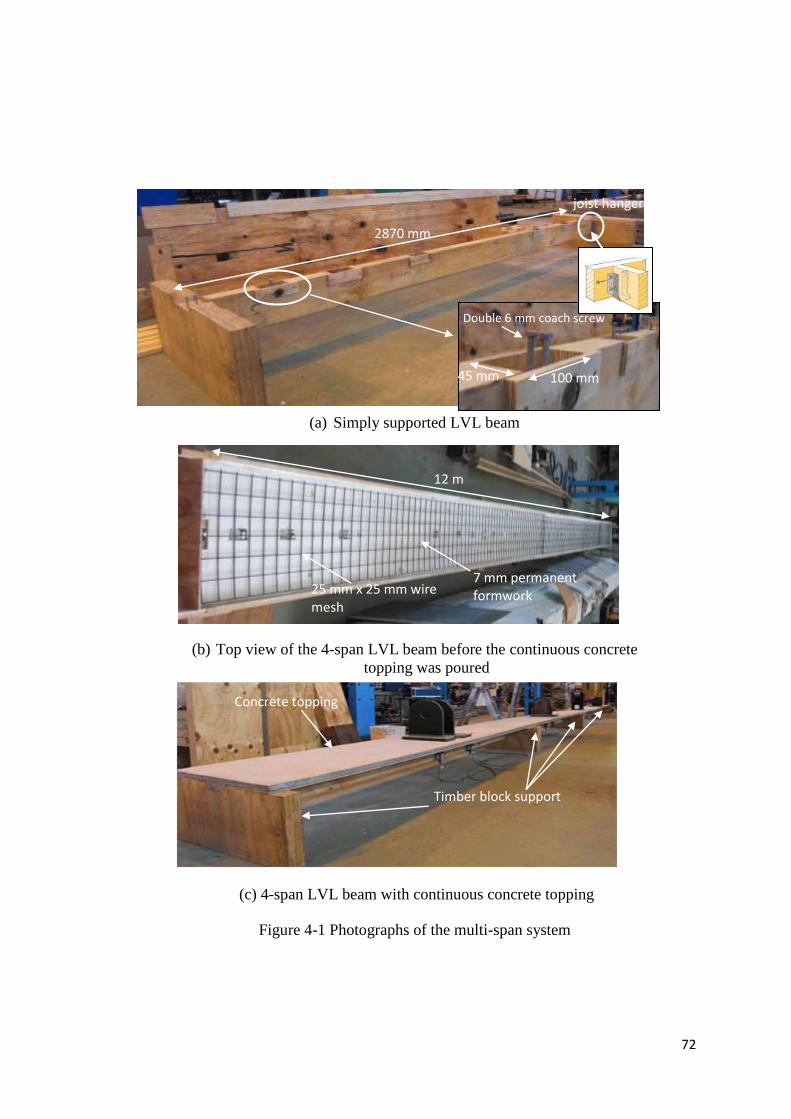
72
(a) Simply supported LVL beam
(b) Top view of the 4-span LVL beam before the continuous concrete
topping was poured
(c) 4-span LVL beam with continuous concrete topping
Figure 4-1 Photographs of the multi-span system
LVL joist
Concrete topping
Concrete topping
Timber block support
Timber block support
Double 6 mm coach screw
100 mm
100 mm
45 mm
45 mm
joist hanger
7 mm permanent formwork
12 m
12 m
25 mm x 25 mm wire mesh
2870 mm
2870 mm
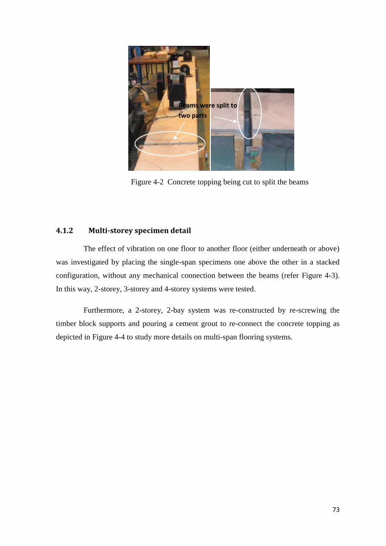
73
Figure 4-2 Concrete topping being cut to split the beams
4.1.2 Multi-storey specimen detail
The effect of vibration on one floor to another floor (either underneath or above)
was investigated by placing the single-span specimens one above the other in a stacked
configuration, without any mechanical connection between the beams (refer Figure 4-3).
In this way, 2-storey, 3-storey and 4-storey systems were tested.
Furthermore, a 2-storey, 2-bay system was re-constructed by re-screwing the
timber block supports and pouring a cement grout to re-connect the concrete topping as
depicted in Figure 4-4 to study more details on multi-span flooring systems.
Beams were split to
two parts
Beams were split to
two parts
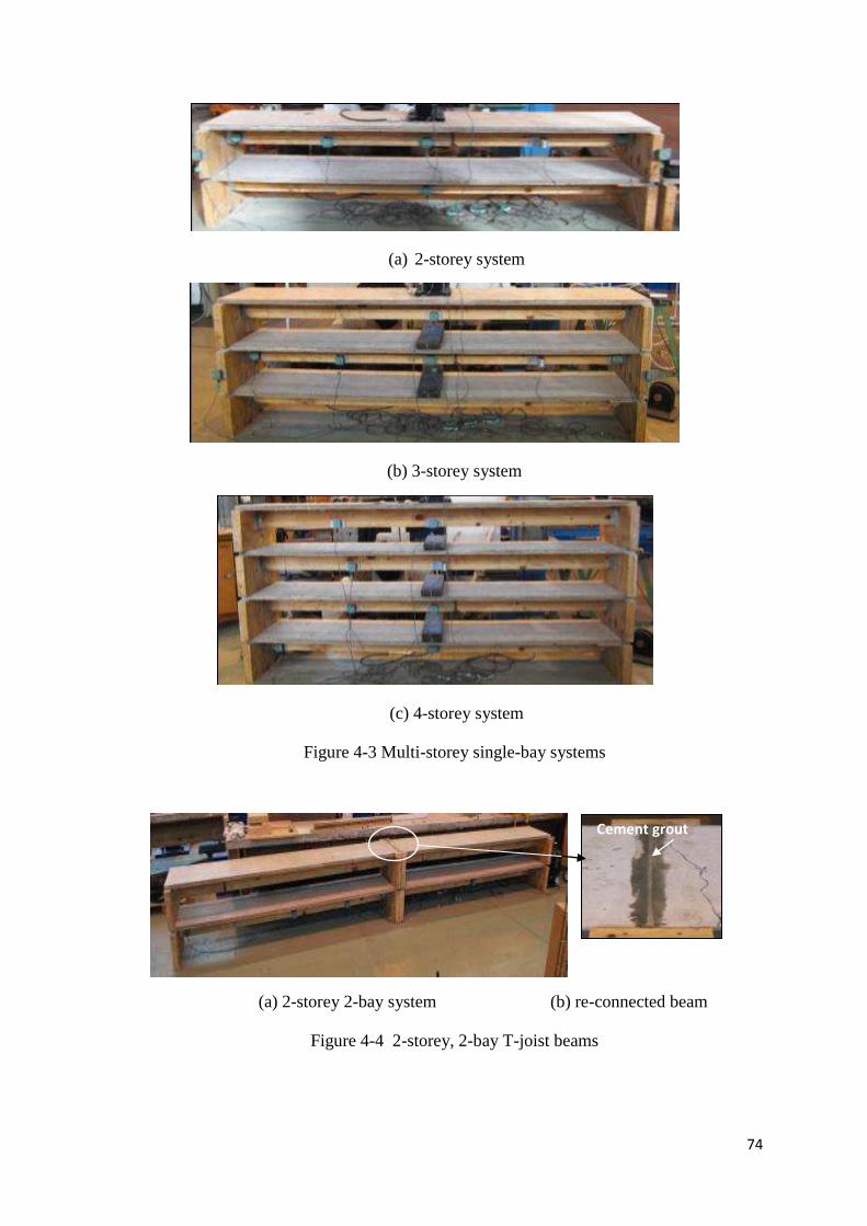
74
(a) 2-storey system
(b) 3-storey system
(c) 4-storey system
Figure 4-3 Multi-storey single-bay systems
(a) 2-storey 2-bay system (b) re-connected beam
Figure 4-4 2-storey, 2-bay T-joist beams
Cement grout
Cement grout
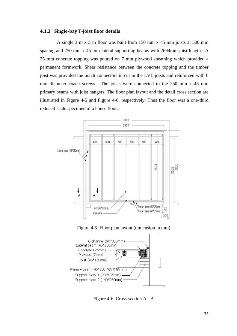
75
4.1.3 Single-bay T-joist floor details
A single 3 m x 3 m floor was built from 150 mm x 45 mm joists at 500 mm
spacing and 250 mm x 45 mm lateral supporting beams with 2694mm joist length. A
25 mm concrete topping was poured on 7 mm plywood sheathing which provided a
permanent formwork. Shear resistance between the concrete topping and the timber
joist was provided the notch connectors in cut in the LVL joists and reinforced with 6
mm diameter coach screws. The joists were connected to the 250 mm x 45 mm
primary beams with joist hangers. The floor plan layout and the detail cross section are
illustrated in Figure 4-5 and Figure 4-6, respectively. Thus the floor was a one-third
reduced-scale specimen of a house floor.
Figure 4-5 Floor plan layout (dimension in mm)
Figure 4-6 Cross-section A - A
A A
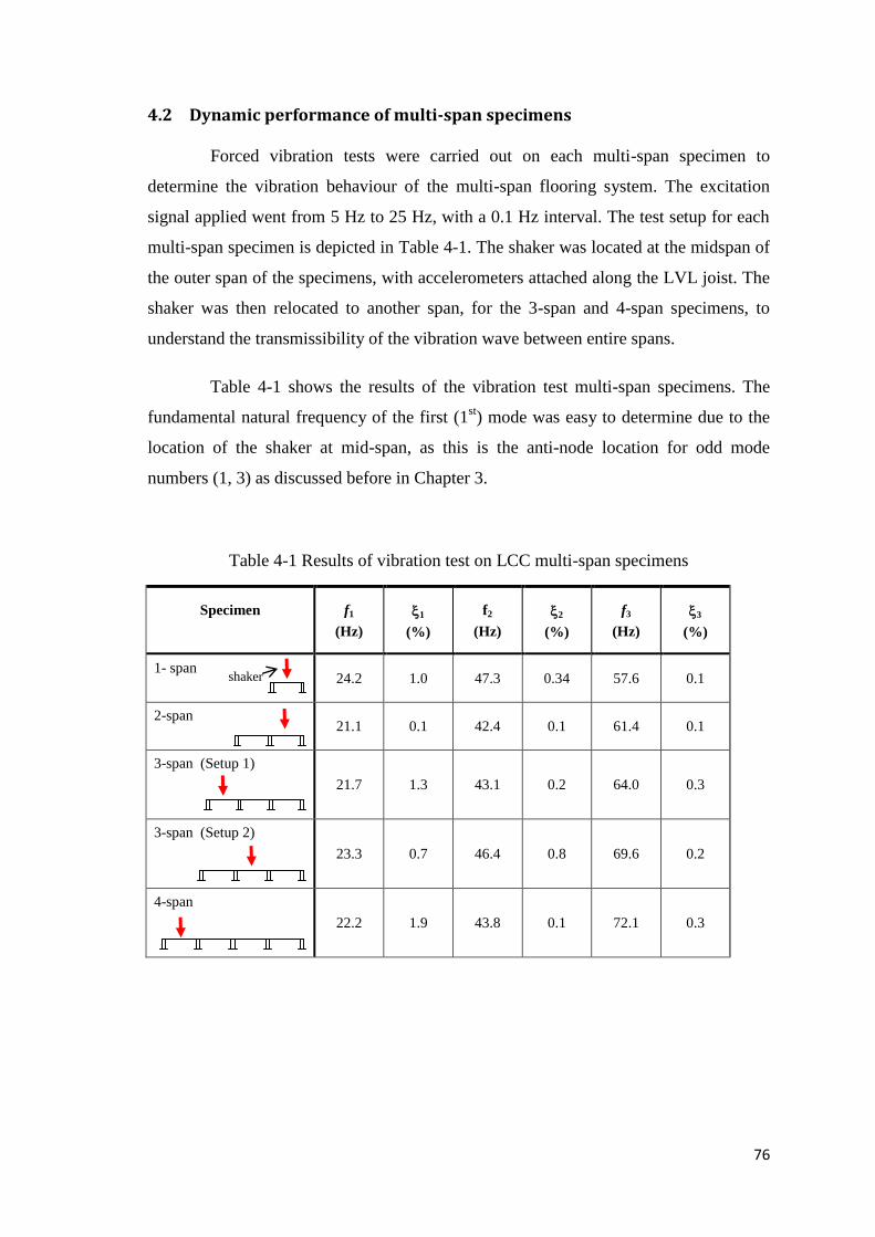
76
4.2 Dynamic performance of multi-span specimens
Forced vibration tests were carried out on each multi-span specimen to
determine the vibration behaviour of the multi-span flooring system. The excitation
signal applied went from 5 Hz to 25 Hz, with a 0.1 Hz interval. The test setup for each
multi-span specimen is depicted in Table 4-1. The shaker was located at the midspan of
the outer span of the specimens, with accelerometers attached along the LVL joist. The
shaker was then relocated to another span, for the 3-span and 4-span specimens, to
understand the transmissibility of the vibration wave between entire spans.
Table 4-1 shows the results of the vibration test multi-span specimens. The
fundamental natural frequency of the first (1st) mode was easy to determine due to the
location of the shaker at mid-span, as this is the anti-node location for odd mode
numbers (1, 3) as discussed before in Chapter 3.
Table 4-1 Results of vibration test on LCC multi-span specimens
Specimen
f1
(Hz)
1
(%)
f2
(Hz)
2
(%)
f3
(Hz)
3
(%)
1- span
24.2 1.0 47.3 0.34 57.6 0.1
2-span
21.1 0.1 42.4 0.1 61.4 0.1
3-span (Setup 1)
21.7 1.3 43.1 0.2 64.0 0.3
3-span (Setup 2)
23.3 0.7 46.4 0.8 69.6 0.2
4-span
22.2 1.9 43.8 0.1 72.1 0.3
shaker
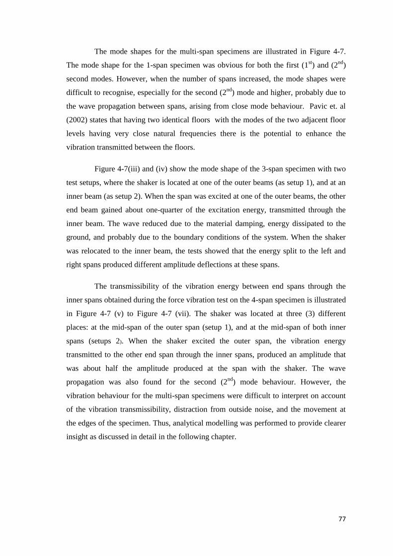
77
The mode shapes for the multi-span specimens are illustrated in Figure 4-7.
The mode shape for the 1-span specimen was obvious for both the first (1st) and (2
nd)
second modes. However, when the number of spans increased, the mode shapes were
difficult to recognise, especially for the second (2nd
) mode and higher, probably due to
the wave propagation between spans, arising from close mode behaviour. Pavic et. al
(2002) states that having two identical floors with the modes of the two adjacent floor
levels having very close natural frequencies there is the potential to enhance the
vibration transmitted between the floors.
Figure 4-7(iii) and (iv) show the mode shape of the 3-span specimen with two
test setups, where the shaker is located at one of the outer beams (as setup 1), and at an
inner beam (as setup 2). When the span was excited at one of the outer beams, the other
end beam gained about one-quarter of the excitation energy, transmitted through the
inner beam. The wave reduced due to the material damping, energy dissipated to the
ground, and probably due to the boundary conditions of the system. When the shaker
was relocated to the inner beam, the tests showed that the energy split to the left and
right spans produced different amplitude deflections at these spans.
The transmissibility of the vibration energy between end spans through the
inner spans obtained during the force vibration test on the 4-span specimen is illustrated
in Figure 4-7 (v) to Figure 4-7 (vii). The shaker was located at three (3) different
places: at the mid-span of the outer span (setup 1), and at the mid-span of both inner
spans (setups 2). When the shaker excited the outer span, the vibration energy
transmitted to the other end span through the inner spans, produced an amplitude that
was about half the amplitude produced at the span with the shaker. The wave
propagation was also found for the second (2nd
) mode behaviour. However, the
vibration behaviour for the multi-span specimens were difficult to interpret on account
of the vibration transmissibility, distraction from outside noise, and the movement at
the edges of the specimen. Thus, analytical modelling was performed to provide clearer
insight as discussed in detail in the following chapter.
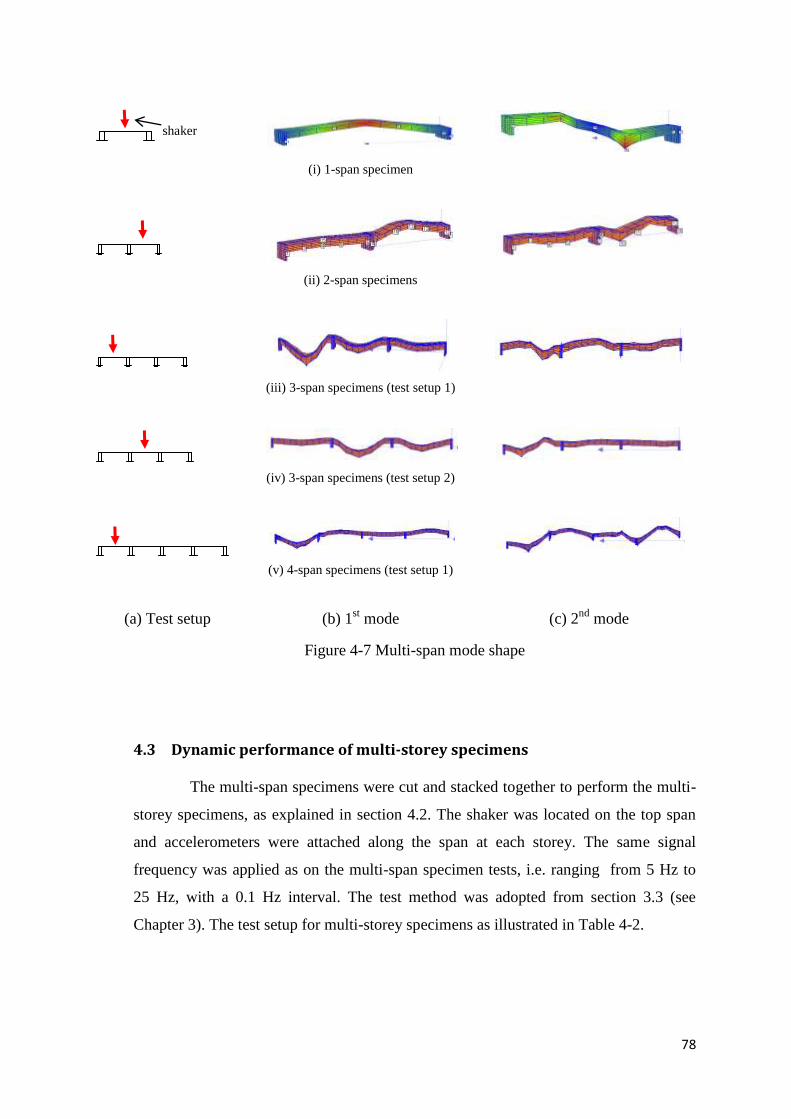
78
(i) 1-span specimen
(ii) 2-span specimens
(iii) 3-span specimens (test setup 1)
(iv) 3-span specimens (test setup 2)
(v) 4-span specimens (test setup 1)
(a) Test setup (b) 1st mode (c) 2
nd mode
Figure 4-7 Multi-span mode shape
4.3 Dynamic performance of multi-storey specimens
The multi-span specimens were cut and stacked together to perform the multi-
storey specimens, as explained in section 4.2. The shaker was located on the top span
and accelerometers were attached along the span at each storey. The same signal
frequency was applied as on the multi-span specimen tests, i.e. ranging from 5 Hz to
25 Hz, with a 0.1 Hz interval. The test method was adopted from section 3.3 (see
Chapter 3). The test setup for multi-storey specimens as illustrated in Table 4-2.
shaker
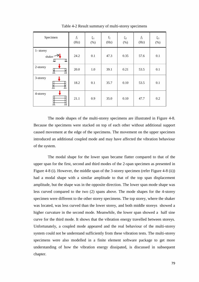
79
Table 4-2 Result summary of multi-storey specimens
Specimen
f1
(Hz)
1
(%)
f2
(Hz)
2
(%)
f3
(Hz)
3
(%)
1- storey
24.2 0.1 47.3 0.35 57.6 0.1
2-storey
20.0 1.0 39.1 0.21 53.5 0.1
3-storey
18.2 0.1 35.7 0.10 53.5 0.1
4-storey
21.1 0.9 35.0 0.10 47.7 0.2
The mode shapes of the multi-storey specimens are illustrated in Figure 4-8.
Because the specimens were stacked on top of each other without additional support
caused movement at the edge of the specimens. The movement on the upper specimen
introduced an additional coupled mode and may have affected the vibration behaviour
of the system.
The modal shape for the lower span became flatter compared to that of the
upper span for the first, second and third modes of the 2-span specimen as presented in
Figure 4-8 (i). However, the middle span of the 3-storey specimen (refer Figure 4-8 (ii))
had a modal shape with a similar amplitude to that of the top span displacement
amplitude, but the shape was in the opposite direction. The lower span mode shape was
less curved compared to the two (2) spans above. The mode shapes for the 4-storey
specimen were different to the other storey specimens. The top storey, where the shaker
was located, was less curved than the lower storey, and both middle storeys showed a
higher curvature in the second mode. Meanwhile, the lower span showed a half sine
curve for the third mode. It shows that the vibration energy travelled between storeys.
Unfortunately, a coupled mode appeared and the real behaviour of the multi-storey
system could not be understand sufficiently from these vibration tests. The multi-storey
specimens were also modelled in a finite element software package to get more
understanding of how the vibration energy dissipated, is discussed in subsequent
chapter.
shaker
80
(i) 2-storey specimen
(ii) 3-storey specimen
(iii) 4-storey specimen
(a) Test
setup (b) 1st mode (c) 2
nd mode (d) 3
rd mode
Figure 4-8 Multi-storey mode shape
4.4 Dynamic performance of a single-bay floor
A larger scale specimen was built to investigate the vibration behaviour of an
LCC flooring system. A reduced-scale 3 m x 3 m LCC floor was built and tested by
electrodynamic shaker to obtain the natural frequencies and mode shapes of the
specimen. Details of the specimens is explained in section 4.1.3. In a similar method to
that for the full-scale LCC specimen (refer Chapter 3), the accelerometers were placed
at the mid-span of the each joist across the floor as illustrated in Figure 4-9. The shaker
was first located at the middle point on the floor and later relocated to one-third of the
floor length, in order to determine the asymmetric and symmetric modes.
Masses were selected that matched the shaker mass and placed on the floor
over each joist at mid span. The natural frequency of the system noticeably decreased.
The addition of masses is shown in Figure 6.10 to decrease the resonance frequency of
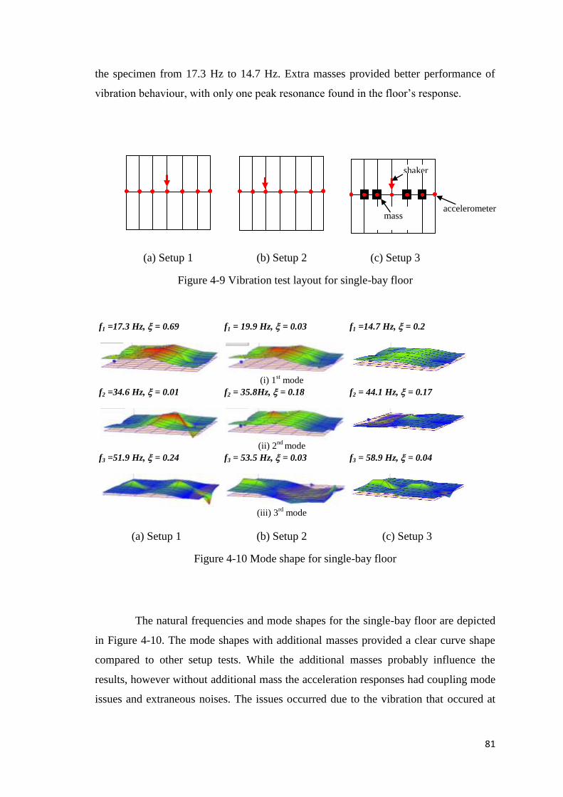
81
the specimen from 17.3 Hz to 14.7 Hz. Extra masses provided better performance of
vibration behaviour, with only one peak resonance found in the floor’s response.
(a) Setup 1 (b) Setup 2 (c) Setup 3
Figure 4-9 Vibration test layout for single-bay floor
f1 =17.3 Hz, = 0.69
f1 = 19.9 Hz, = 0.03
f1 =14.7 Hz, = 0.2
(i) 1
st mode
f2 =34.6 Hz, = 0.01
f2 = 35.8Hz, = 0.18
f2 = 44.1 Hz, = 0.17
(ii) 2nd
mode
f3 =51.9 Hz, = 0.24
f3 = 53.5 Hz, = 0.03
f3 = 58.9 Hz, = 0.04
(iii) 3
rd mode
(a) Setup 1 (b) Setup 2 (c) Setup 3
Figure 4-10 Mode shape for single-bay floor
The natural frequencies and mode shapes for the single-bay floor are depicted
in Figure 4-10. The mode shapes with additional masses provided a clear curve shape
compared to other setup tests. While the additional masses probably influence the
results, however without additional mass the acceleration responses had coupling mode
issues and extraneous noises. The issues occurred due to the vibration that occured at
shaker
accelerometer mass
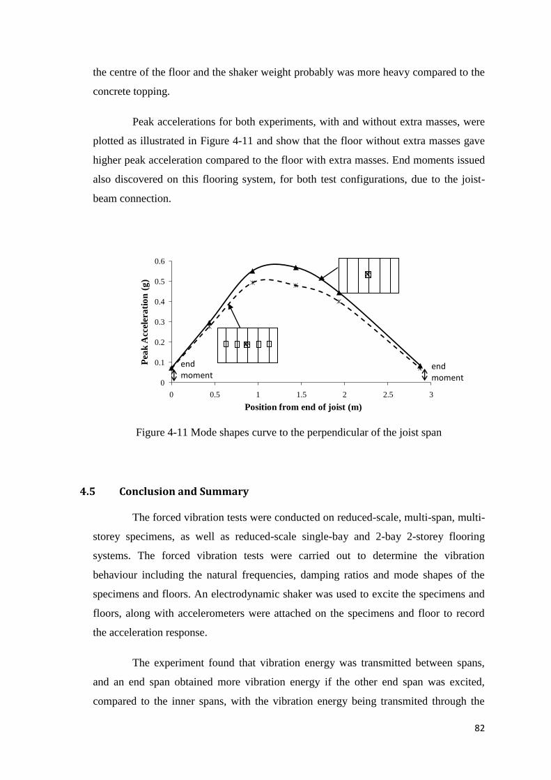
82
the centre of the floor and the shaker weight probably was more heavy compared to the
concrete topping.
Peak accelerations for both experiments, with and without extra masses, were
plotted as illustrated in Figure 4-11 and show that the floor without extra masses gave
higher peak acceleration compared to the floor with extra masses. End moments issued
also discovered on this flooring system, for both test configurations, due to the joist-
beam connection.
Figure 4-11 Mode shapes curve to the perpendicular of the joist span
4.5 Conclusion and Summary
The forced vibration tests were conducted on reduced-scale, multi-span, multi-
storey specimens, as well as reduced-scale single-bay and 2-bay 2-storey flooring
systems. The forced vibration tests were carried out to determine the vibration
behaviour including the natural frequencies, damping ratios and mode shapes of the
specimens and floors. An electrodynamic shaker was used to excite the specimens and
floors, along with accelerometers were attached on the specimens and floor to record
the acceleration response.
The experiment found that vibration energy was transmitted between spans,
and an end span obtained more vibration energy if the other end span was excited,
compared to the inner spans, with the vibration energy being transmited through the
0
0.1
0.2
0.3
0.4
0.5
0.6
0 0.5 1 1.5 2 2.5 3
Pea
k A
ccel
era
tio
n (
g)
Position from end of joist (m)
x
x
6
5
6
5
x
x
end moment
end
moment
end moment
end
moment

83
inner spans. The transmitted vibration energy provided close modes between spans or
storeys, with the mode shapes difficult to identify, especially for 2nd
and 3rd
modes,
however the global mode shapes could be recognised. This situation applied for both
multi-span and multi-storey flooring systems. Detailed investigation on the vibration
transmissibility is discussed in the next chapter where the results of finite element
modelling are presented.
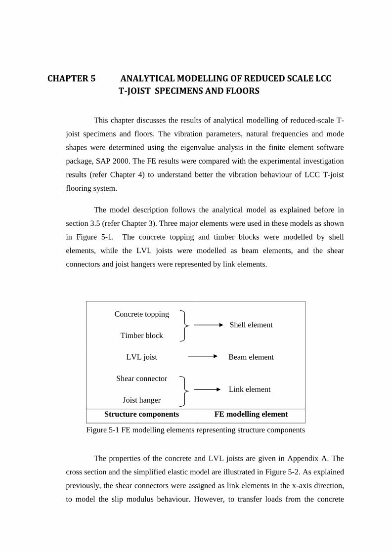
CHAPTER 5 ANALYTICAL MODELLING OF REDUCED SCALE LCC
T-JOIST SPECIMENS AND FLOORS
This chapter discusses the results of analytical modelling of reduced-scale T-
joist specimens and floors. The vibration parameters, natural frequencies and mode
shapes were determined using the eigenvalue analysis in the finite element software
package, SAP 2000. The FE results were compared with the experimental investigation
results (refer Chapter 4) to understand better the vibration behaviour of LCC T-joist
flooring system.
The model description follows the analytical model as explained before in
section 3.5 (refer Chapter 3). Three major elements were used in these models as shown
in Figure 5-1. The concrete topping and timber blocks were modelled by shell
elements, while the LVL joists were modelled as beam elements, and the shear
connectors and joist hangers were represented by link elements.
Concrete topping
Shell element
Timber block
LVL joist Beam element
Shear connector
Link element
Joist hanger
Structure components FE modelling element
Figure 5-1 FE modelling elements representing structure components
The properties of the concrete and LVL joists are given in Appendix A. The
cross section and the simplified elastic model are illustrated in Figure 5-2. As explained
previously, the shear connectors were assigned as link elements in the x-axis direction,
to model the slip modulus behaviour. However, to transfer loads from the concrete
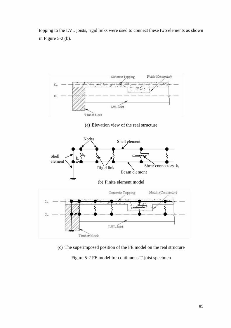
85
topping to the LVL joists, rigid links were used to connect these two elements as shown
in Figure 5-2 (b).
(a) Elevation view of the real structure
(b) Finite element model
(c) The superimposed position of the FE model on the real structure
Figure 5-2 FE model for continuous T-joist specimen
kj ks
Nodes
Beam element Rigid link
Shell element
Shear connectors, kc
Shell
element
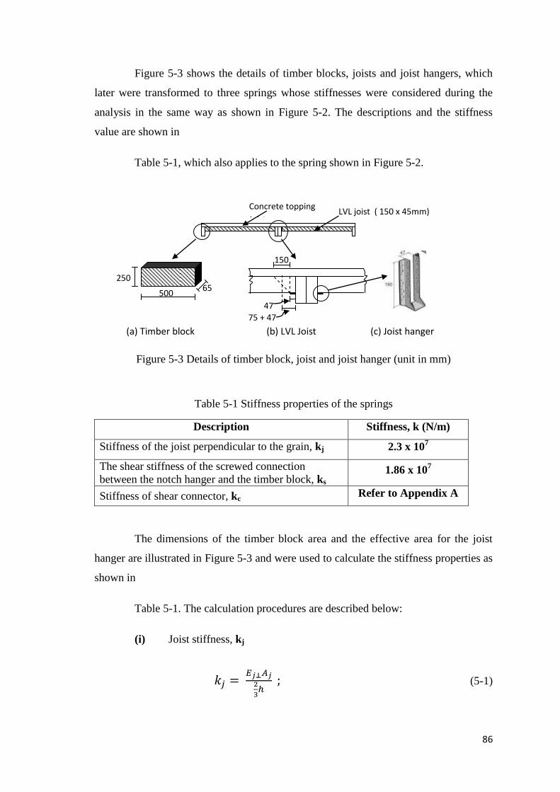
86
Figure 5-3 shows the details of timber blocks, joists and joist hangers, which
later were transformed to three springs whose stiffnesses were considered during the
analysis in the same way as shown in Figure 5-2. The descriptions and the stiffness
value are shown in
Table 5-1, which also applies to the spring shown in Figure 5-2.
Figure 5-3 Details of timber block, joist and joist hanger (unit in mm)
Table 5-1 Stiffness properties of the springs
Description Stiffness, k (N/m)
Stiffness of the joist perpendicular to the grain, kj 2.3 x 10⁷
The shear stiffness of the screwed connection
between the notch hanger and the timber block, ks
1.86 x 10⁷
Stiffness of shear connector, kc Refer to Appendix A
The dimensions of the timber block area and the effective area for the joist
hanger are illustrated in Figure 5-3 and were used to calculate the stiffness properties as
shown in
Table 5-1. The calculation procedures are described below:
(i) Joist stiffness, kj
(5-1)
LVL joist ( 150 x 45mm)
(a) Timber block
Concrete topping
Joist
500 65
250
(b) LVL Joist (c) Joist hanger
75 + 47
150
47
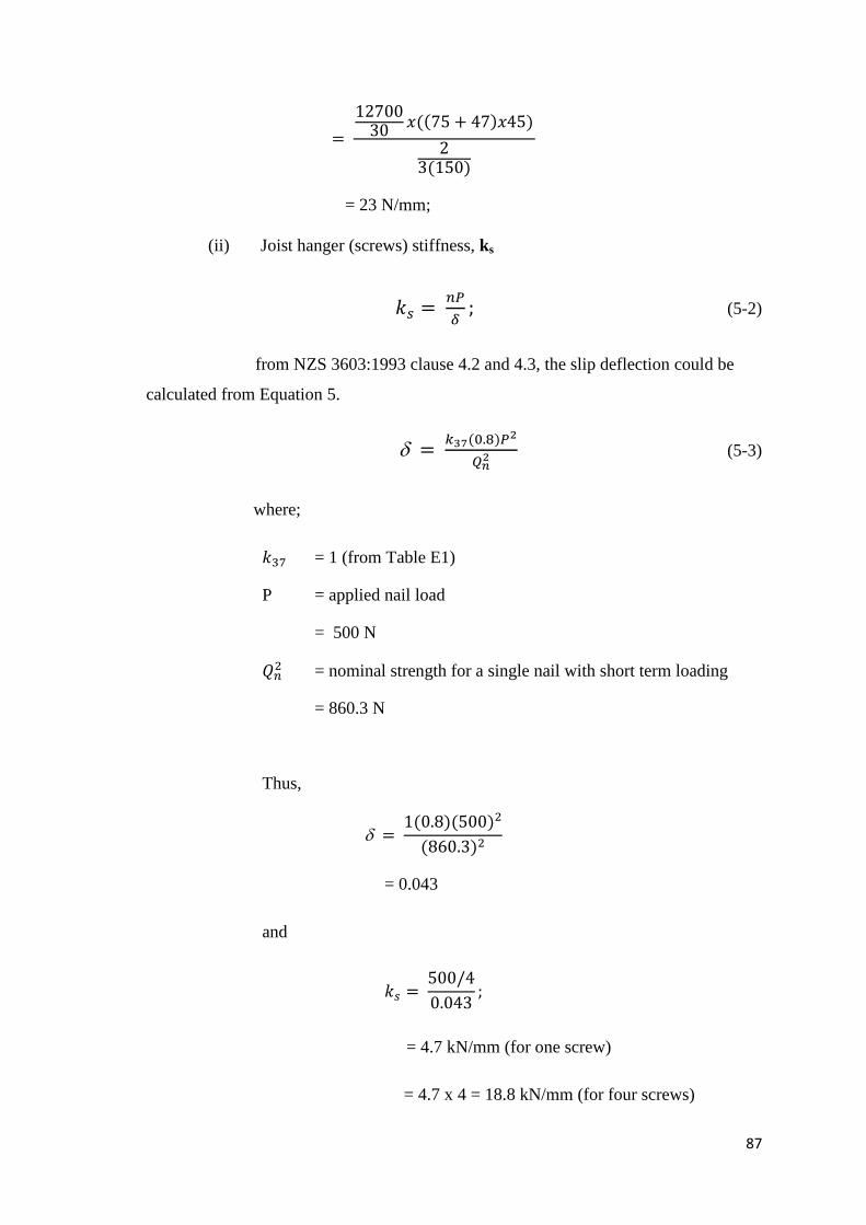
87
= 23 N/mm;
(ii) Joist hanger (screws) stiffness, ks
(5-2)
from NZS 3603:1993 clause 4.2 and 4.3, the slip deflection could be
calculated from Equation 5.
(5-3)
where;
= 1 (from Table E1)
P = applied nail load
= 500 N
= nominal strength for a single nail with short term loading
= 860.3 N
Thus,
= 0.043
and
= 4.7 kN/mm (for one screw)
= 4.7 x 4 = 18.8 kN/mm (for four screws)
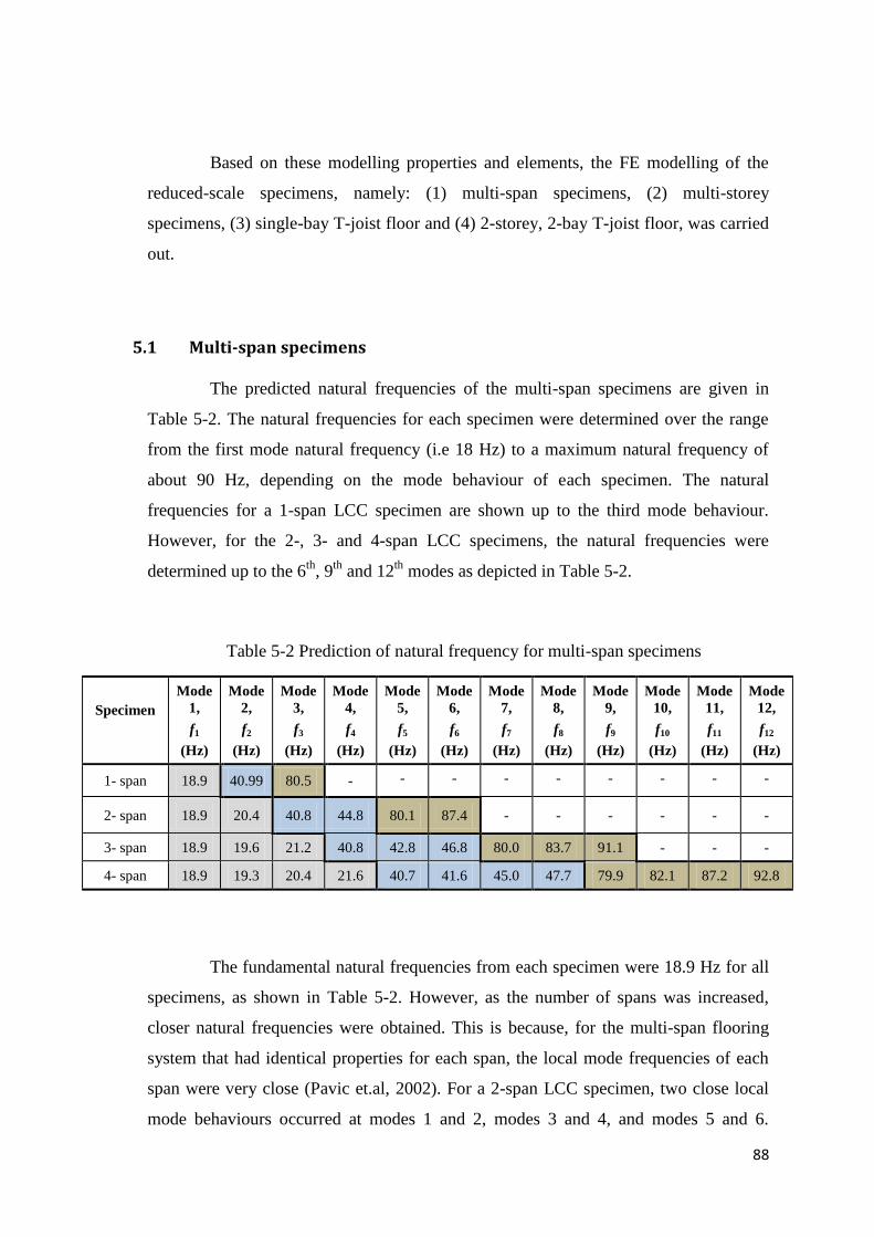
88
Based on these modelling properties and elements, the FE modelling of the
reduced-scale specimens, namely: (1) multi-span specimens, (2) multi-storey
specimens, (3) single-bay T-joist floor and (4) 2-storey, 2-bay T-joist floor, was carried
out.
5.1 Multi-span specimens
The predicted natural frequencies of the multi-span specimens are given in
Table 5-2. The natural frequencies for each specimen were determined over the range
from the first mode natural frequency (i.e 18 Hz) to a maximum natural frequency of
about 90 Hz, depending on the mode behaviour of each specimen. The natural
frequencies for a 1-span LCC specimen are shown up to the third mode behaviour.
However, for the 2-, 3- and 4-span LCC specimens, the natural frequencies were
determined up to the 6th
, 9th
and 12th
modes as depicted in Table 5-2.
Table 5-2 Prediction of natural frequency for multi-span specimens
Specimen
Mode
1,
f1
(Hz)
Mode
2,
f2
(Hz)
Mode
3,
f3
(Hz)
Mode
4,
f4
(Hz)
Mode
5,
f5
(Hz)
Mode
6,
f6
(Hz)
Mode
7,
f7
(Hz)
Mode
8,
f8
(Hz)
Mode
9,
f9
(Hz)
Mode
10,
f10
(Hz)
Mode
11,
f11
(Hz)
Mode
12,
f12
(Hz)
1- span 18.9 40.99 80.5 - - - - - - - - -
2- span 18.9 20.4 40.8 44.8 80.1 87.4 - - - - - -
3- span 18.9 19.6 21.2 40.8 42.8 46.8 80.0 83.7 91.1 - - -
4- span 18.9 19.3 20.4 21.6 40.7 41.6 45.0 47.7 79.9 82.1 87.2 92.8
The fundamental natural frequencies from each specimen were 18.9 Hz for all
specimens, as shown in Table 5-2. However, as the number of spans was increased,
closer natural frequencies were obtained. This is because, for the multi-span flooring
system that had identical properties for each span, the local mode frequencies of each
span were very close (Pavic et.al, 2002). For a 2-span LCC specimen, two close local
mode behaviours occurred at modes 1 and 2, modes 3 and 4, and modes 5 and 6.
89
Comparable behaviour occurred for 3- and 4-span LCC specimens. However, for a 3-
span LCC specimen, three close local modes were determined and for the 4-span LCC
specimen, four close local modes were predicted. Thus, the number of close local
modes was proportional to the number of spans.
The mode shape behaviour of the multi-span specimens is illustrated from
Figure 5-4 to Figure 5-9. Theoretically, the first mode behaviour shows a half-sine
curve and the second mode shows a full-sine curve. The third and forth modes have the
shape of one and half sine curves and two full-sine curves, respectively. These
particular shapes were also shown by the 1-span LCC specimen (refer to Figure 5-4).
The mode shape behaviours changed when the 1-span LCC specimens had an
adjacent span. The local mode behaviour of each span dominated the global mode
behaviour of the system for each mode. For a 2-span LCC specimen, the mode shape
behaviour was a half-sine curve for modes 1 and 2, for each span. However, the
position of the curves were different. For the first mode, span 1 showed a hogging
shape while span 2 was sagging, and both spans had a hogging shape for the second
mode. The full-sine curve appeared at the third and fourth modes. Both spans had
similar properties, thus the mode shape behaviour was also comparable.
On the other hand, the 3- and 4-span LCC specimens showed different
behaviour for the mode shapes. The fundamental natural frequencies of both specimens
show that the mode shapes were almost similar for each span (refer to Figure 5-6 and
Figure 5-8). However, at some points, either the inner span(s) or the outer spans
dominated the global mode of the system. Figure 5-6 and Figure 5-7 show that the inner
span for a 3-span LCC specimen governed the global mode at modes 3, 6 and 9 and the
rest of the modes were dominated by the outer spans, except for mode 1. Referring to
Figure 5-8 and Figure 5-9, the even numbered global modes were governed either by
the inner spans or by the outer spans. The odd numbered global mode shapes show an
almost similar curve deflection for each span, but in opposite deformation.
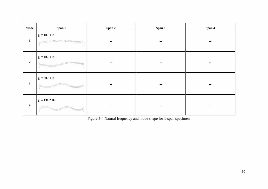
90
Mode Span 1 Span 2 Span 3 Span 4
1
f1 = 18.9 Hz
- - -
2
f2 = 40.9 Hz
- - -
3
f3 = 80.5 Hz
- - -
4
f4 = 130.2 Hz
- - -
Figure 5-4 Natural frequency and mode shape for 1-span specimen
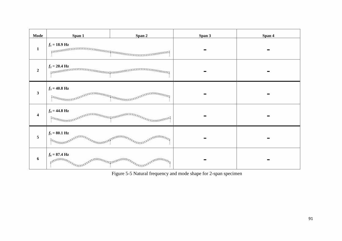
91
Mode Span 1 Span 2 Span 3 Span 4
1 f1 = 18.9 Hz
- -
2 f2 = 20.4 Hz
- -
3
f3 = 40.8 Hz
- -
4 f4 = 44.8 Hz
- -
5 f5 = 80.1 Hz
- -
6 f6 = 87.4 Hz
- -
Figure 5-5 Natural frequency and mode shape for 2-span specimen
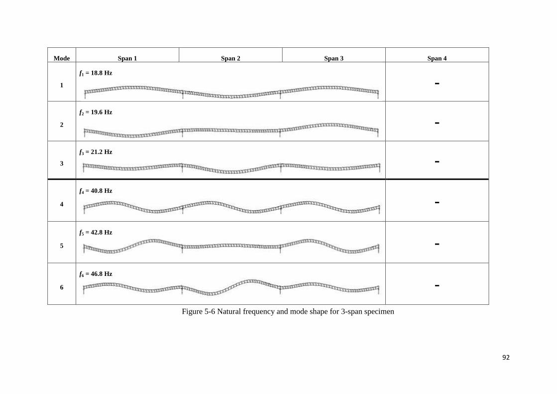
92
Mode Span 1 Span 2 Span 3 Span 4
1
f1 = 18.8 Hz
-
2
f2 = 19.6 Hz
-
3
f3 = 21.2 Hz
-
4
f4 = 40.8 Hz
-
5
f5 = 42.8 Hz
-
6
f6 = 46.8 Hz
-
Figure 5-6 Natural frequency and mode shape for 3-span specimen
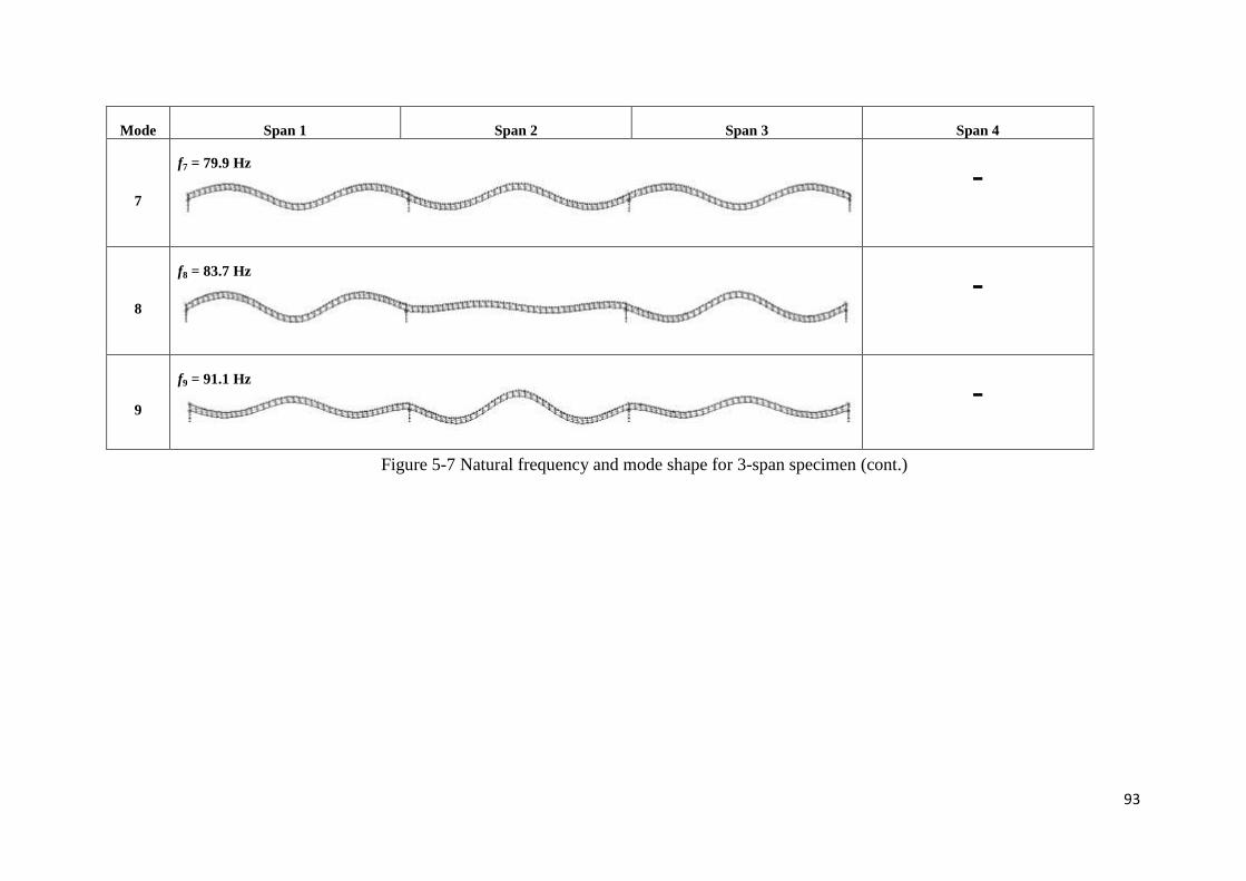
93
Mode Span 1 Span 2 Span 3 Span 4
7
f7 = 79.9 Hz
-
8
f8 = 83.7 Hz
-
9
f9 = 91.1 Hz
-
Figure 5-7 Natural frequency and mode shape for 3-span specimen (cont.)
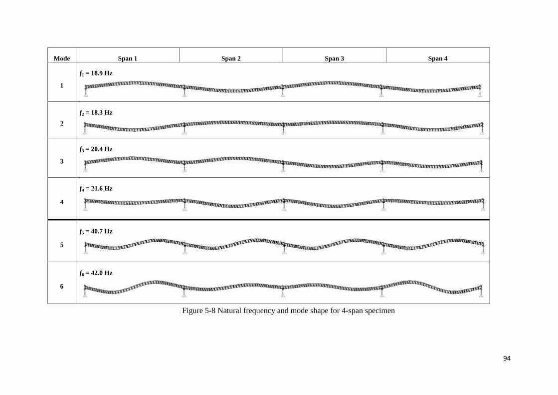
94
Mode Span 1 Span 2 Span 3 Span 4
1
f1 = 18.9 Hz
2
f2 = 18.3 Hz
3
f3 = 20.4 Hz
4
f4 = 21.6 Hz
5
f5 = 40.7 Hz
6
f6 = 42.0 Hz
Figure 5-8 Natural frequency and mode shape for 4-span specimen
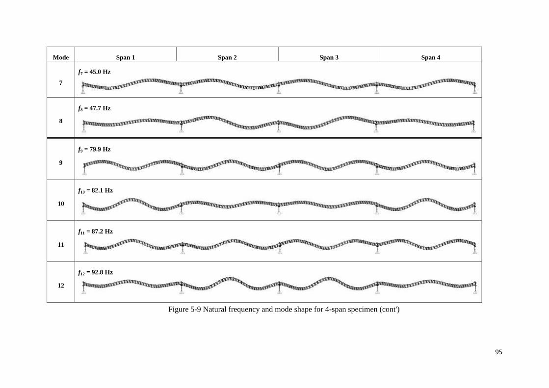
95
Mode Span 1 Span 2 Span 3 Span 4
7
f7 = 45.0 Hz
8
f8 = 47.7 Hz
9
f9 = 79.9 Hz
10
f10 = 82.1 Hz
11
f11 = 87.2 Hz
12
f12 = 92.8 Hz
Figure 5-9 Natural frequency and mode shape for 4-span specimen (cont')
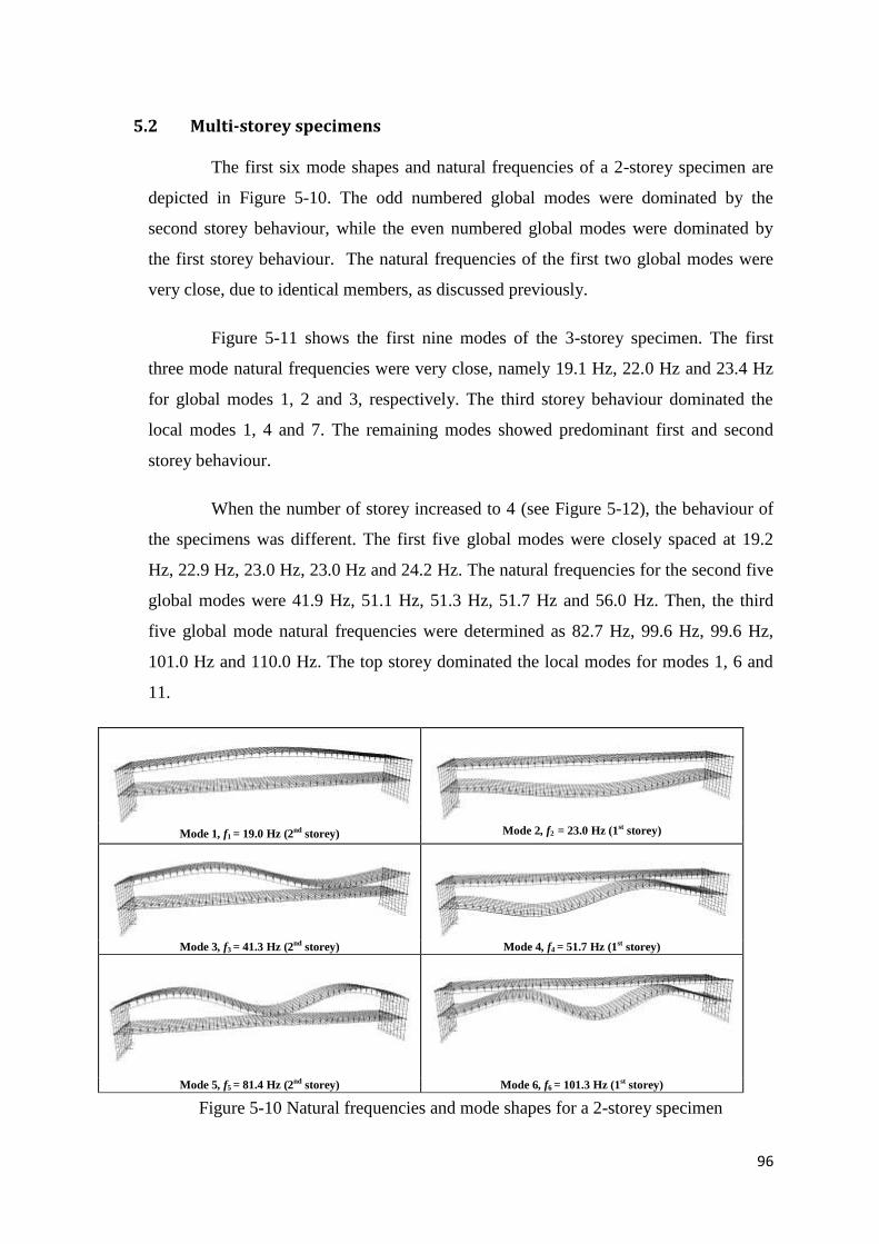
96
5.2 Multi-storey specimens
The first six mode shapes and natural frequencies of a 2-storey specimen are
depicted in Figure 5-10. The odd numbered global modes were dominated by the
second storey behaviour, while the even numbered global modes were dominated by
the first storey behaviour. The natural frequencies of the first two global modes were
very close, due to identical members, as discussed previously.
Figure 5-11 shows the first nine modes of the 3-storey specimen. The first
three mode natural frequencies were very close, namely 19.1 Hz, 22.0 Hz and 23.4 Hz
for global modes 1, 2 and 3, respectively. The third storey behaviour dominated the
local modes 1, 4 and 7. The remaining modes showed predominant first and second
storey behaviour.
When the number of storey increased to 4 (see Figure 5-12), the behaviour of
the specimens was different. The first five global modes were closely spaced at 19.2
Hz, 22.9 Hz, 23.0 Hz, 23.0 Hz and 24.2 Hz. The natural frequencies for the second five
global modes were 41.9 Hz, 51.1 Hz, 51.3 Hz, 51.7 Hz and 56.0 Hz. Then, the third
five global mode natural frequencies were determined as 82.7 Hz, 99.6 Hz, 99.6 Hz,
101.0 Hz and 110.0 Hz. The top storey dominated the local modes for modes 1, 6 and
11.
Mode 1, f1 = 19.0 Hz (2nd storey) Mode 2, f2 = 23.0 Hz (1st storey)
Mode 3, f3 = 41.3 Hz (2nd storey) Mode 4, f4 = 51.7 Hz (1st storey)
Mode 5, f5 = 81.4 Hz (2nd storey) Mode 6, f6 = 101.3 Hz (1st storey)
Figure 5-10 Natural frequencies and mode shapes for a 2-storey specimen
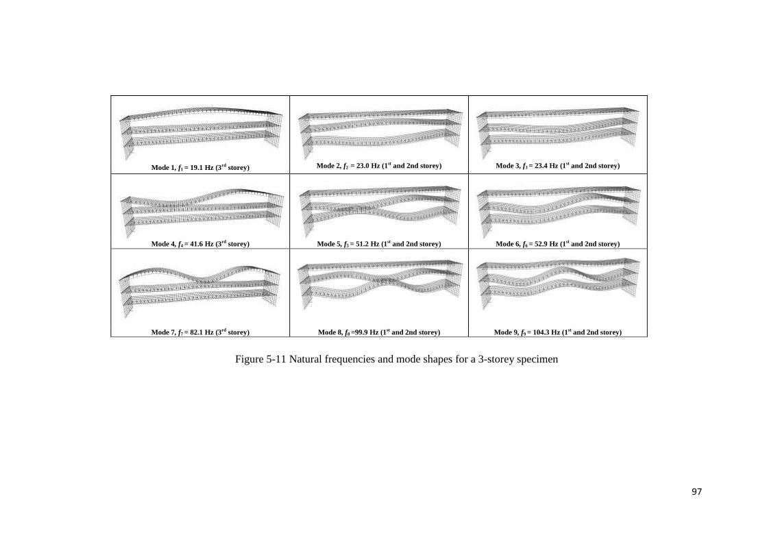
97
Mode 1, f1 = 19.1 Hz (3rd storey) Mode 2, f2 = 23.0 Hz (1st and 2nd storey) Mode 3, f3 = 23.4 Hz (1st and 2nd storey)
Mode 4, f4 = 41.6 Hz (3rd storey) Mode 5, f5 = 51.2 Hz (1st and 2nd storey) Mode 6, f6 = 52.9 Hz (1st and 2nd storey)
Mode 7, f7 = 82.1 Hz (3rd storey) Mode 8, f8 =99.9 Hz (1st and 2nd storey) Mode 9, f9 = 104.3 Hz (1st and 2nd storey)
Figure 5-11 Natural frequencies and mode shapes for a 3-storey specimen
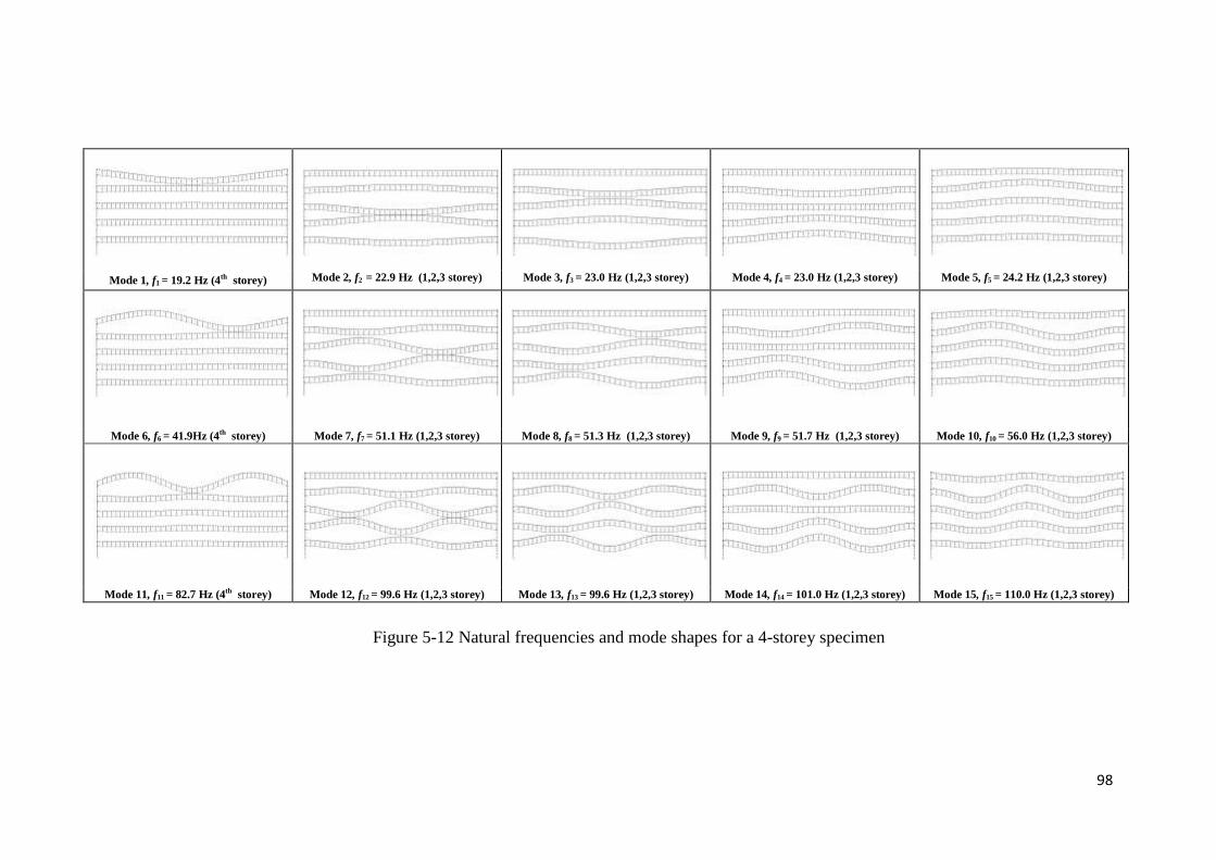
98
Mode 1, f1 = 19.2 Hz (4th storey) Mode 2, f2 = 22.9 Hz (1,2,3 storey) Mode 3, f3 = 23.0 Hz (1,2,3 storey) Mode 4, f4 = 23.0 Hz (1,2,3 storey) Mode 5, f5 = 24.2 Hz (1,2,3 storey)
Mode 6, f6 = 41.9Hz (4th storey) Mode 7, f7 = 51.1 Hz (1,2,3 storey) Mode 8, f8 = 51.3 Hz (1,2,3 storey) Mode 9, f9 = 51.7 Hz (1,2,3 storey) Mode 10, f10 = 56.0 Hz (1,2,3 storey)
Mode 11, f11 = 82.7 Hz (4th storey) Mode 12, f12 = 99.6 Hz (1,2,3 storey) Mode 13, f13 = 99.6 Hz (1,2,3 storey) Mode 14, f14 = 101.0 Hz (1,2,3 storey) Mode 15, f15 = 110.0 Hz (1,2,3 storey)
Figure 5-12 Natural frequencies and mode shapes for a 4-storey specimen
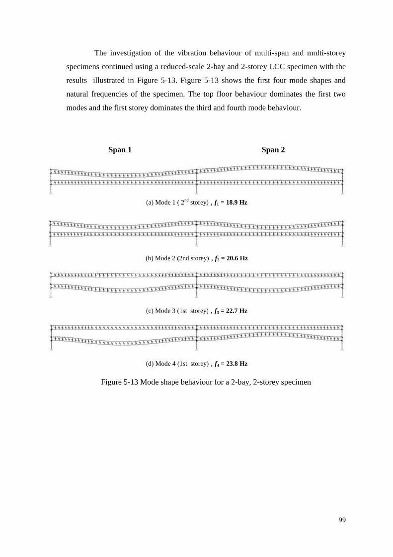
99
The investigation of the vibration behaviour of multi-span and multi-storey
specimens continued using a reduced-scale 2-bay and 2-storey LCC specimen with the
results illustrated in Figure 5-13. Figure 5-13 shows the first four mode shapes and
natural frequencies of the specimen. The top floor behaviour dominates the first two
modes and the first storey dominates the third and fourth mode behaviour.
Span 1 Span 2
(a) Mode 1 ( 2
nd storey) , f1 = 18.9 Hz
(b) Mode 2 (2nd storey) , f2 = 20.6 Hz
(c) Mode 3 (1st storey) , f3 = 22.7 Hz
(d) Mode 4 (1st storey) , f4 = 23.8 Hz
Figure 5-13 Mode shape behaviour for a 2-bay, 2-storey specimen
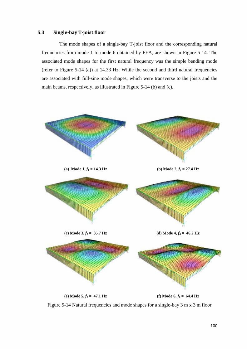
100
5.3 Single-bay T-joist floor
The mode shapes of a single-bay T-joist floor and the corresponding natural
frequencies from mode 1 to mode 6 obtained by FEA, are shown in Figure 5-14. The
associated mode shapes for the first natural frequency was the simple bending mode
(refer to Figure 5-14 (a)) at 14.33 Hz. While the second and third natural frequencies
are associated with full-sine mode shapes, which were transverse to the joists and the
main beams, respectively, as illustrated in Figure 5-14 (b) and (c).
(a) Mode 1, f1 = 14.3 Hz (b) Mode 2, f2 = 27.4 Hz
(c) Mode 3, f3 = 35.7 Hz (d) Mode 4, f4 = 46.2 Hz
(e) Mode 5, f5 = 47.1 Hz (f) Mode 6, f6 = 64.4 Hz
Figure 5-14 Natural frequencies and mode shapes for a single-bay 3 m x 3 m floor
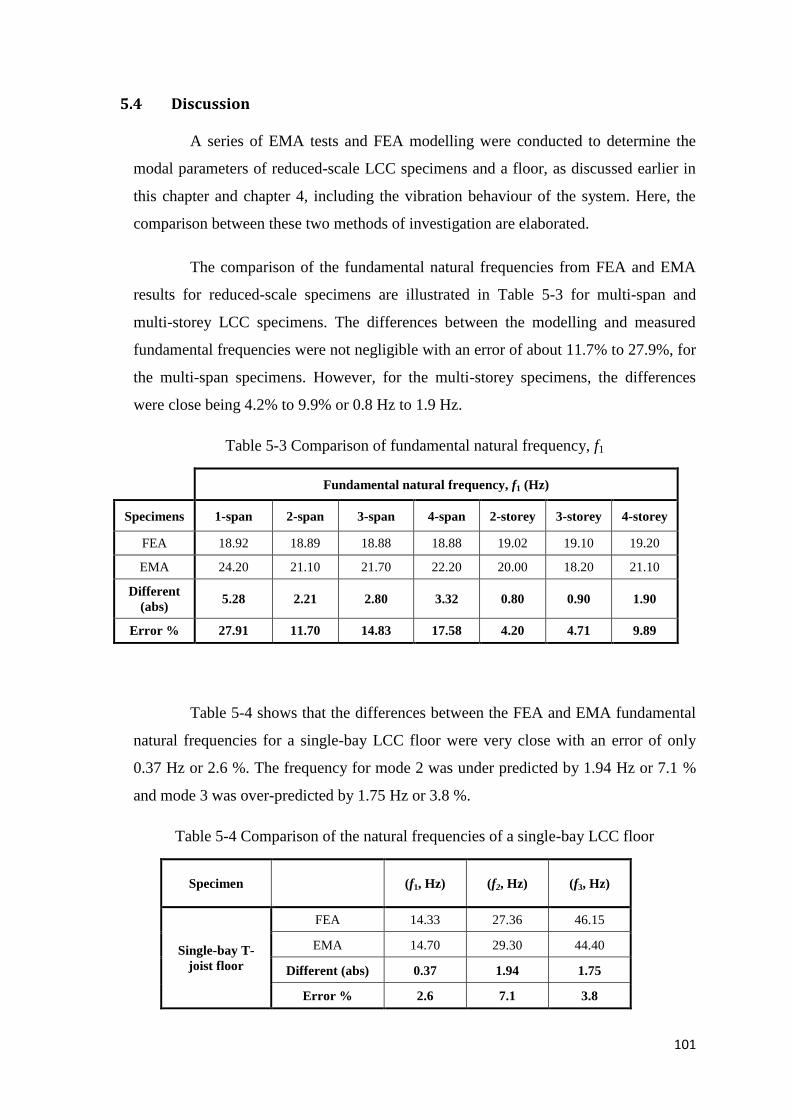
101
5.4 Discussion
A series of EMA tests and FEA modelling were conducted to determine the
modal parameters of reduced-scale LCC specimens and a floor, as discussed earlier in
this chapter and chapter 4, including the vibration behaviour of the system. Here, the
comparison between these two methods of investigation are elaborated.
The comparison of the fundamental natural frequencies from FEA and EMA
results for reduced-scale specimens are illustrated in Table 5-3 for multi-span and
multi-storey LCC specimens. The differences between the modelling and measured
fundamental frequencies were not negligible with an error of about 11.7% to 27.9%, for
the multi-span specimens. However, for the multi-storey specimens, the differences
were close being 4.2% to 9.9% or 0.8 Hz to 1.9 Hz.
Table 5-3 Comparison of fundamental natural frequency, f1
Fundamental natural frequency, f1 (Hz)
Specimens 1-span 2-span 3-span 4-span 2-storey 3-storey 4-storey
FEA 18.92 18.89 18.88 18.88 19.02 19.10 19.20
EMA 24.20 21.10 21.70 22.20 20.00 18.20 21.10
Different
(abs) 5.28 2.21 2.80 3.32 0.80 0.90 1.90
Error % 27.91 11.70 14.83 17.58 4.20 4.71 9.89
Table 5-4 shows that the differences between the FEA and EMA fundamental
natural frequencies for a single-bay LCC floor were very close with an error of only
0.37 Hz or 2.6 %. The frequency for mode 2 was under predicted by 1.94 Hz or 7.1 %
and mode 3 was over-predicted by 1.75 Hz or 3.8 %.
Table 5-4 Comparison of the natural frequencies of a single-bay LCC floor
Specimen
(f1, Hz) (f2, Hz) (f3, Hz)
Single-bay T-
joist floor
FEA 14.33 27.36 46.15
EMA 14.70 29.30 44.40
Different (abs) 0.37 1.94 1.75
Error % 2.6 7.1 3.8
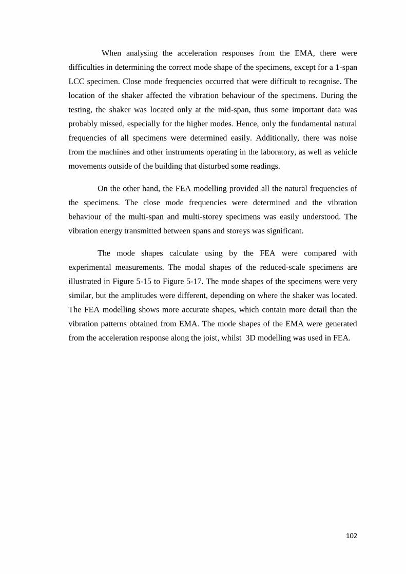
102
When analysing the acceleration responses from the EMA, there were
difficulties in determining the correct mode shape of the specimens, except for a 1-span
LCC specimen. Close mode frequencies occurred that were difficult to recognise. The
location of the shaker affected the vibration behaviour of the specimens. During the
testing, the shaker was located only at the mid-span, thus some important data was
probably missed, especially for the higher modes. Hence, only the fundamental natural
frequencies of all specimens were determined easily. Additionally, there was noise
from the machines and other instruments operating in the laboratory, as well as vehicle
movements outside of the building that disturbed some readings.
On the other hand, the FEA modelling provided all the natural frequencies of
the specimens. The close mode frequencies were determined and the vibration
behaviour of the multi-span and multi-storey specimens was easily understood. The
vibration energy transmitted between spans and storeys was significant.
The mode shapes calculate using by the FEA were compared with
experimental measurements. The modal shapes of the reduced-scale specimens are
illustrated in Figure 5-15 to Figure 5-17. The mode shapes of the specimens were very
similar, but the amplitudes were different, depending on where the shaker was located.
The FEA modelling shows more accurate shapes, which contain more detail than the
vibration patterns obtained from EMA. The mode shapes of the EMA were generated
from the acceleration response along the joist, whilst 3D modelling was used in FEA.
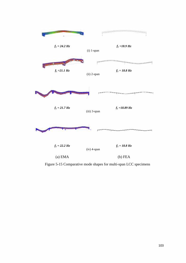
103
f1 = 24.2 Hz f1 =18.9 Hz
(i) 1-span
f1 =21.1 Hz f1 = 18.8 Hz
(ii) 2-span
f1 = 21.7 Hz f1 =18.89 Hz
(iii) 3-span
f1 = 22.2 Hz f1 = 18.8 Hz (iv) 4-span
(a) EMA (b) FEA
Figure 5-15 Comparative mode shapes for multi-span LCC specimens
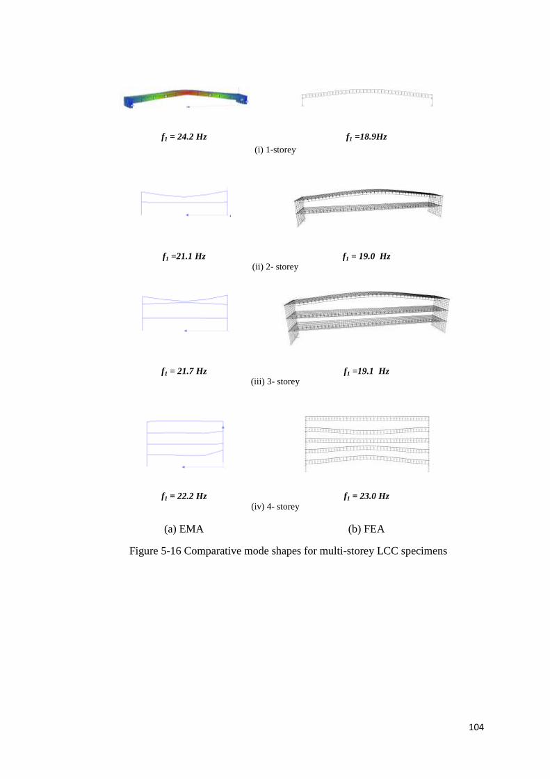
104
f1 = 24.2 Hz f1 =18.9Hz
(i) 1-storey
f1 =21.1 Hz f1 = 19.0 Hz
(ii) 2- storey
f1 = 21.7 Hz f1 =19.1 Hz
(iii) 3- storey
f1 = 22.2 Hz f1 = 23.0 Hz (iv) 4- storey
(a) EMA (b) FEA
Figure 5-16 Comparative mode shapes for multi-storey LCC specimens
105
f1 =14.7 Hz f1 =14.33 Hz
(i) mode 1
f2 = 29.3 Hz f2 = 27.4 Hz
(ii) Mode 2
f3 = 44.4 Hz f3 = 46.2 Hz
(iii) Mode 3
(a) EMA (b) FEA
Figure 5-17 Comparative mode shapes for the single-bay LCC floor
5.5 Summary and Conclusions
The analytical modelling was performed to validate the experimental modal
analysis (EMA) results using the modal analysis method in the SAP 2000 software
package, for reduced-scale LCC T-joist specimens and floor. Only natural frequencies
and mode shape were determined during the modal analysis. The vibration behaviour of
the specimens and floor were more easily understood compared to the EMA, due to the
effect of close mode frequencies.
The modal analysis showed local mode frequencies were very close and the
number of close local modes was proportional to the number of spans due to the
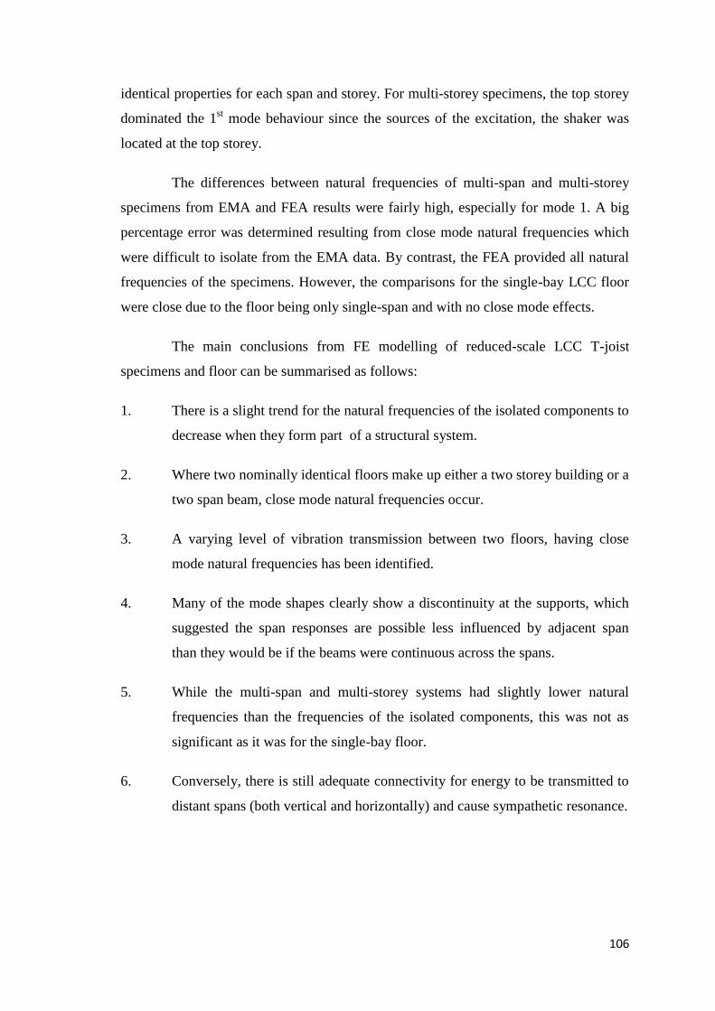
106
identical properties for each span and storey. For multi-storey specimens, the top storey
dominated the 1st mode behaviour since the sources of the excitation, the shaker was
located at the top storey.
The differences between natural frequencies of multi-span and multi-storey
specimens from EMA and FEA results were fairly high, especially for mode 1. A big
percentage error was determined resulting from close mode natural frequencies which
were difficult to isolate from the EMA data. By contrast, the FEA provided all natural
frequencies of the specimens. However, the comparisons for the single-bay LCC floor
were close due to the floor being only single-span and with no close mode effects.
The main conclusions from FE modelling of reduced-scale LCC T-joist
specimens and floor can be summarised as follows:
1. There is a slight trend for the natural frequencies of the isolated components to
decrease when they form part of a structural system.
2. Where two nominally identical floors make up either a two storey building or a
two span beam, close mode natural frequencies occur.
3. A varying level of vibration transmission between two floors, having close
mode natural frequencies has been identified.
4. Many of the mode shapes clearly show a discontinuity at the supports, which
suggested the span responses are possible less influenced by adjacent span
than they would be if the beams were continuous across the spans.
5. While the multi-span and multi-storey systems had slightly lower natural
frequencies than the frequencies of the isolated components, this was not as
significant as it was for the single-bay floor.
6. Conversely, there is still adequate connectivity for energy to be transmitted to
distant spans (both vertical and horizontally) and cause sympathetic resonance.
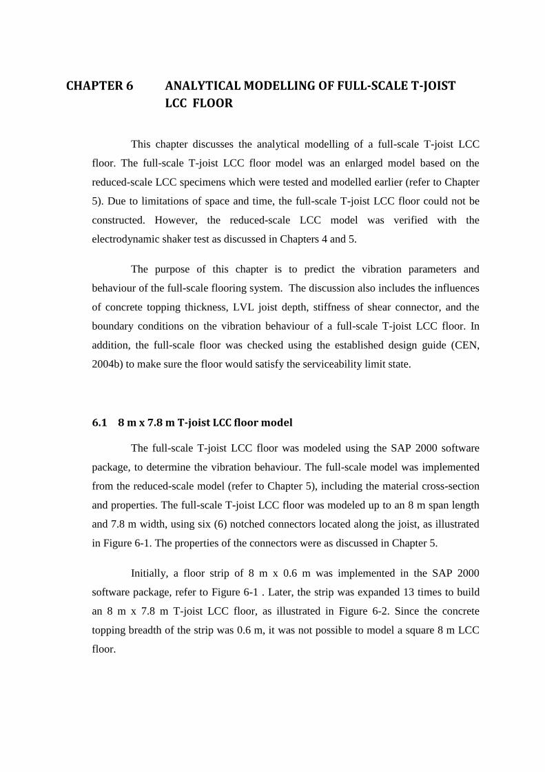
CHAPTER 6 ANALYTICAL MODELLING OF FULL-SCALE T-JOIST
LCC FLOOR
This chapter discusses the analytical modelling of a full-scale T-joist LCC
floor. The full-scale T-joist LCC floor model was an enlarged model based on the
reduced-scale LCC specimens which were tested and modelled earlier (refer to Chapter
5). Due to limitations of space and time, the full-scale T-joist LCC floor could not be
constructed. However, the reduced-scale LCC model was verified with the
electrodynamic shaker test as discussed in Chapters 4 and 5.
The purpose of this chapter is to predict the vibration parameters and
behaviour of the full-scale flooring system. The discussion also includes the influences
of concrete topping thickness, LVL joist depth, stiffness of shear connector, and the
boundary conditions on the vibration behaviour of a full-scale T-joist LCC floor. In
addition, the full-scale floor was checked using the established design guide (CEN,
2004b) to make sure the floor would satisfy the serviceability limit state.
6.1 8 m x 7.8 m T-joist LCC floor model
The full-scale T-joist LCC floor was modeled using the SAP 2000 software
package, to determine the vibration behaviour. The full-scale model was implemented
from the reduced-scale model (refer to Chapter 5), including the material cross-section
and properties. The full-scale T-joist LCC floor was modeled up to an 8 m span length
and 7.8 m width, using six (6) notched connectors located along the joist, as illustrated
in Figure 6-1. The properties of the connectors were as discussed in Chapter 5.
Initially, a floor strip of 8 m x 0.6 m was implemented in the SAP 2000
software package, refer to Figure 6-1 . Later, the strip was expanded 13 times to build
an 8 m x 7.8 m T-joist LCC floor, as illustrated in Figure 6-2. Since the concrete
topping breadth of the strip was 0.6 m, it was not possible to model a square 8 m LCC
floor.
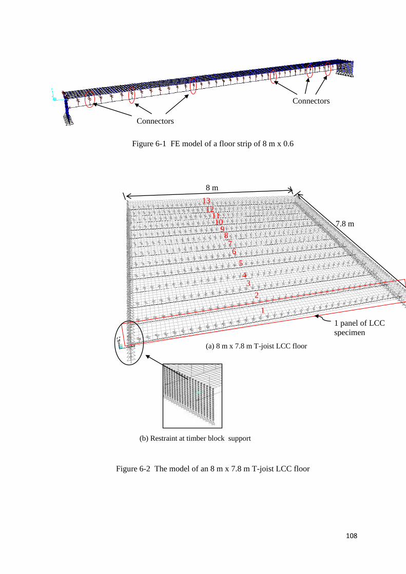
108
Figure 6-1 FE model of a floor strip of 8 m x 0.6
Figure 6-2 The model of an 8 m x 7.8 m T-joist LCC floor
Connectors
Connectors
7.8 m
8 m
2
7
1 panel of LCC
specimen
1
3 4
5
6
8 9
10
13 12
11
(b) Restraint at timber block support
(a) 8 m x 7.8 m T-joist LCC floor
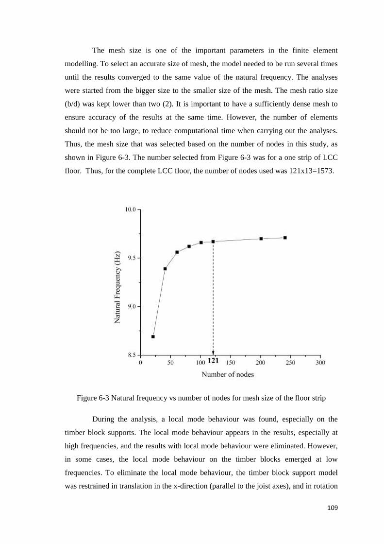
109
The mesh size is one of the important parameters in the finite element
modelling. To select an accurate size of mesh, the model needed to be run several times
until the results converged to the same value of the natural frequency. The analyses
were started from the bigger size to the smaller size of the mesh. The mesh ratio size
(b/d) was kept lower than two (2). It is important to have a sufficiently dense mesh to
ensure accuracy of the results at the same time. However, the number of elements
should not be too large, to reduce computational time when carrying out the analyses.
Thus, the mesh size that was selected based on the number of nodes in this study, as
shown in Figure 6-3. The number selected from Figure 6-3 was for a one strip of LCC
floor. Thus, for the complete LCC floor, the number of nodes used was 121x13=1573.
Figure 6-3 Natural frequency vs number of nodes for mesh size of the floor strip
During the analysis, a local mode behaviour was found, especially on the
timber block supports. The local mode behaviour appears in the results, especially at
high frequencies, and the results with local mode behaviour were eliminated. However,
in some cases, the local mode behaviour on the timber blocks emerged at low
frequencies. To eliminate the local mode behaviour, the timber block support model
was restrained in translation in the x-direction (parallel to the joist axes), and in rotation
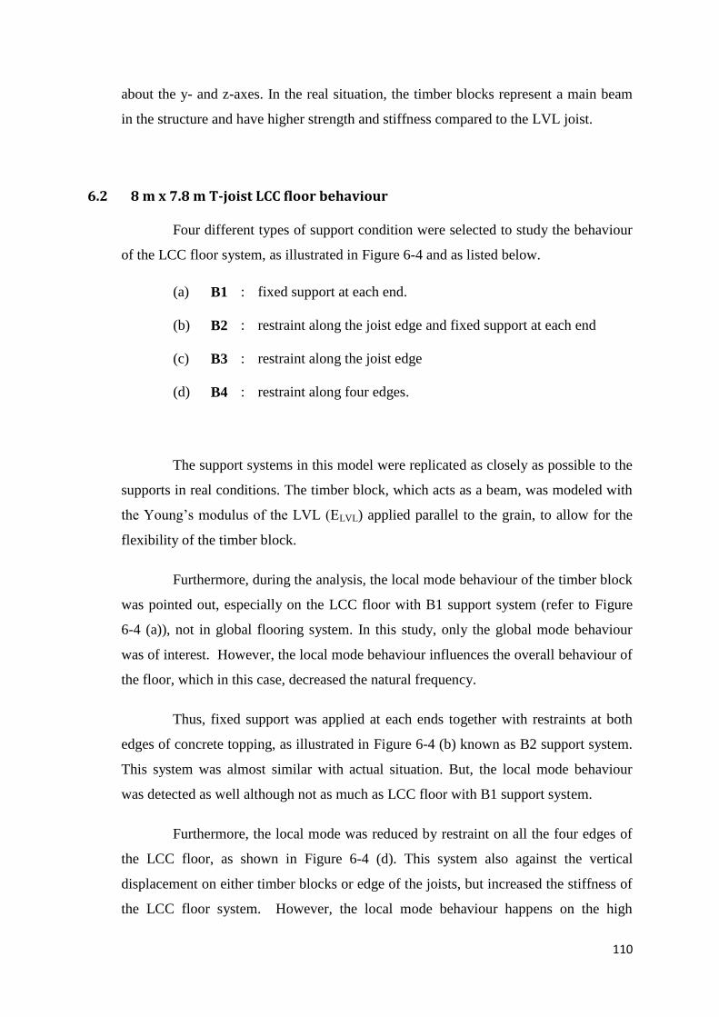
110
about the y- and z-axes. In the real situation, the timber blocks represent a main beam
in the structure and have higher strength and stiffness compared to the LVL joist.
6.2 8 m x 7.8 m T-joist LCC floor behaviour
Four different types of support condition were selected to study the behaviour
of the LCC floor system, as illustrated in Figure 6-4 and as listed below.
(a) B1 : fixed support at each end.
(b) B2 : restraint along the joist edge and fixed support at each end
(c) B3 : restraint along the joist edge
(d) B4 : restraint along four edges.
The support systems in this model were replicated as closely as possible to the
supports in real conditions. The timber block, which acts as a beam, was modeled with
the Young’s modulus of the LVL (ELVL) applied parallel to the grain, to allow for the
flexibility of the timber block.
Furthermore, during the analysis, the local mode behaviour of the timber block
was pointed out, especially on the LCC floor with B1 support system (refer to Figure
6-4 (a)), not in global flooring system. In this study, only the global mode behaviour
was of interest. However, the local mode behaviour influences the overall behaviour of
the floor, which in this case, decreased the natural frequency.
Thus, fixed support was applied at each ends together with restraints at both
edges of concrete topping, as illustrated in Figure 6-4 (b) known as B2 support system.
This system was almost similar with actual situation. But, the local mode behaviour
was detected as well although not as much as LCC floor with B1 support system.
Furthermore, the local mode was reduced by restraint on all the four edges of
the LCC floor, as shown in Figure 6-4 (d). This system also against the vertical
displacement on either timber blocks or edge of the joists, but increased the stiffness of
the LCC floor system. However, the local mode behaviour happens on the high
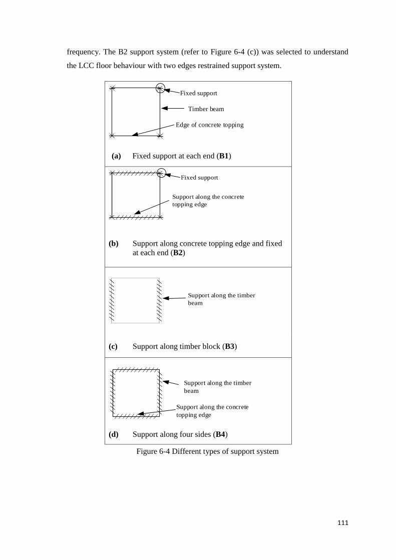
111
frequency. The B2 support system (refer to Figure 6-4 (c)) was selected to understand
the LCC floor behaviour with two edges restrained support system.
Timber beam
Edge of concrete topping
Fixed support
(a) Fixed support at each end (B1)
Support along the concrete
topping edge
Fixed support
(b) Support along concrete topping edge and fixed
at each end (B2)
Support along the timber
beam
(c) Support along timber block (B3)
Support along the concrete
topping edge
Support along the timber
beam
(d) Support along four sides (B4)
Figure 6-4 Different types of support system
112
Figure 6-5 illustrates the natural frequency for first six modes of the LCC floor
with different types of support systems. From the overall results, the LCC floor with B4
support system presents the highest value of natural frequency for all modes, compared
to other support systems. This is because restraint at all the edges increased the stiffness
of the system and increased the natural frequency as well. Also related to this, the floor
with B1 support system had the lowest value of natural frequency due to the diminished
support stiffness.
However, the natural frequencies were close for modes 1 and 2, between 5.88
Hz to 9.12 Hz and 8.61 Hz to 11.28 Hz, respectively. At mode 3, the natural
frequencies were close for except LCC floor with B4 system. The differences of the
natural frequencies were large for higher mode frequencies.
The mode shapes of the LCC floor is illustrated in Figure 6-6 with different
types of support systems. All the behaviour acted as a plate except for the LCC floor
with B3 support system, which acted as a beam. It is because all the three support
systems, B1, B2 and B4 have a restraint at each end and for B2 only restraint along the
timber joist.
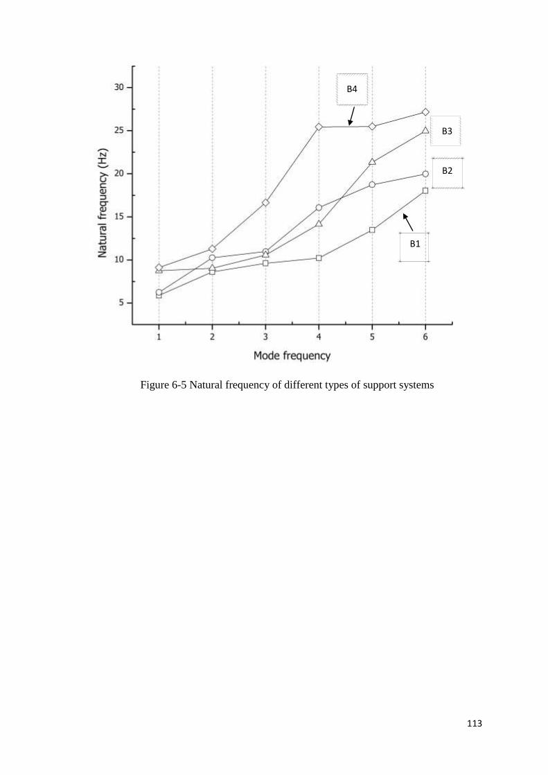
113
Figure 6-5 Natural frequency of different types of support systems
B3
B4
B2
B1
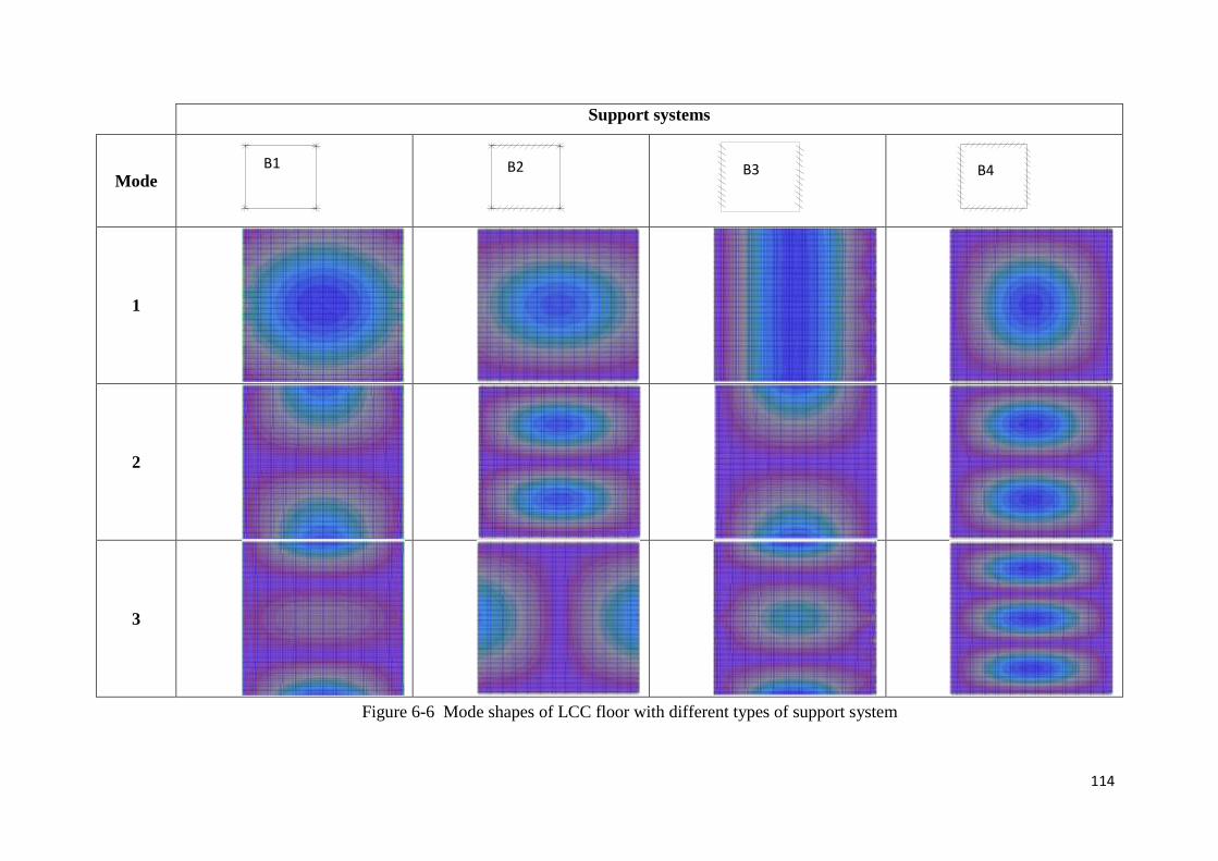
114
Support systems
Mode
1
2
3
Figure 6-6 Mode shapes of LCC floor with different types of support system
B1 B2 B3 B4
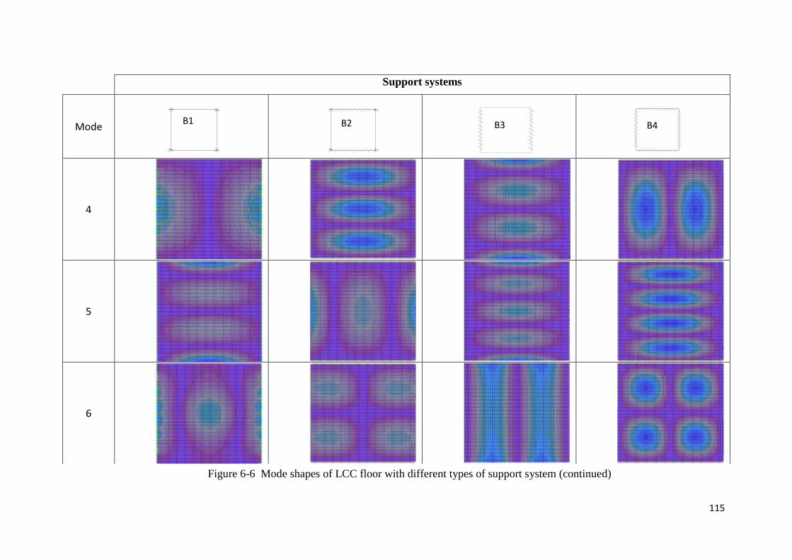
115
Figure 6-6 Mode shapes of LCC floor with different types of support system (continued)
Support systems
Mode
4
5
6
B1 B2 B3 B4
116
6.3 Effect of connector stiffness
Figure 6-7 shows the first mode natural frequency of the full-scale LCC floor
for five different types of connectors. Three connectors were selected as suggested by
Yeoh (2010), with the stiffness of each connector being: (1) K1 = 80.2 kN/mm, (2) K2
= 146 kN/mm and (3) K3 = 247 kN/mm. Additionally two extra stiffnesses were added,
of K0 = 0 kN/mm and K4 = 108 kN/mm to represent no slip and rigid stiffness
connection of the LCC flooring system, respectively. The differences of the connector
stiffnesses were generated between two types of support system, B2 and B4 (refer
section 6.2 for details), with restraint on two side edges and restraint on four side edges,
respectively.
Obviously, the flooring system with restraint on all the edges gave the higher
value of natural frequency, with the increase of the floor stiffness. This behaviour was
also applicable when the connector stiffness was changed. The natural frequency was
rising with the increase of the connector stiffness. However, the differences are small
for mode 1 until mode 4, except for the K0 connector stiffness. It seems clear that
changing the stiffness of connectors did not greatly influence the vibration behaviour of
the LCC floor especially for lower modes (from mode 1 until mode 4). In general
however, the natural frequencies increased equivalent with the connector stiffness. The
behaviour was changed for the higher modes, 5 and 6, as the domination of the higher
stiffnesses were shown especially for the floor with B4 support system.
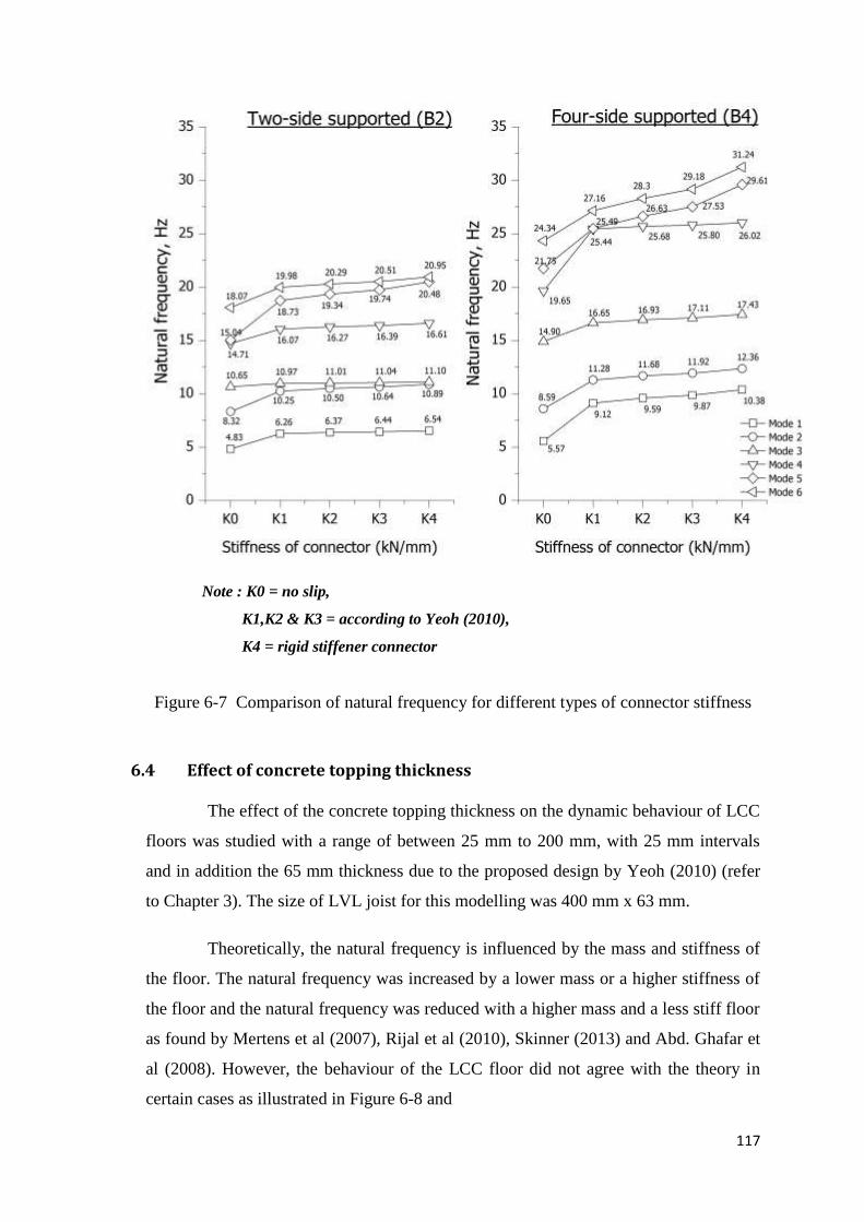
117
Note : K0 = no slip,
K1,K2 & K3 = according to Yeoh (2010),
K4 = rigid stiffener connector
Figure 6-7 Comparison of natural frequency for different types of connector stiffness
6.4 Effect of concrete topping thickness
The effect of the concrete topping thickness on the dynamic behaviour of LCC
floors was studied with a range of between 25 mm to 200 mm, with 25 mm intervals
and in addition the 65 mm thickness due to the proposed design by Yeoh (2010) (refer
to Chapter 3). The size of LVL joist for this modelling was 400 mm x 63 mm.
Theoretically, the natural frequency is influenced by the mass and stiffness of
the floor. The natural frequency was increased by a lower mass or a higher stiffness of
the floor and the natural frequency was reduced with a higher mass and a less stiff floor
as found by Mertens et al (2007), Rijal et al (2010), Skinner (2013) and Abd. Ghafar et
al (2008). However, the behaviour of the LCC floor did not agree with the theory in
certain cases as illustrated in Figure 6-8 and
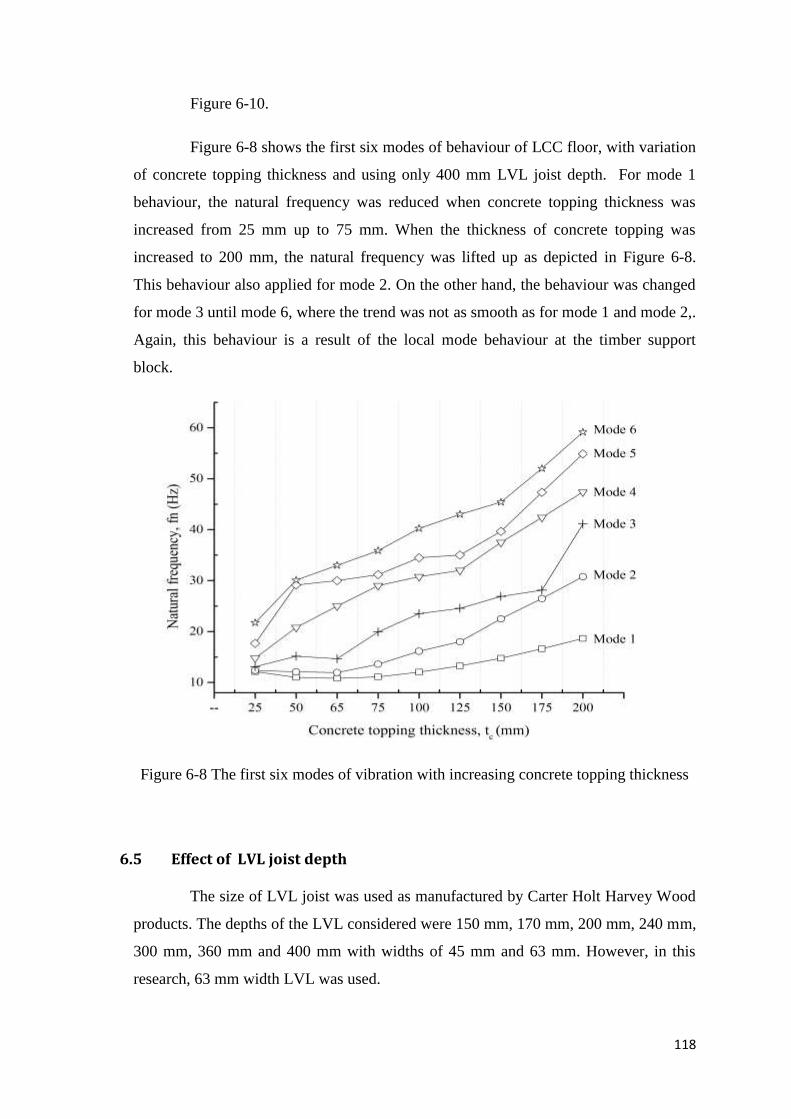
118
Figure 6-10.
Figure 6-8 shows the first six modes of behaviour of LCC floor, with variation
of concrete topping thickness and using only 400 mm LVL joist depth. For mode 1
behaviour, the natural frequency was reduced when concrete topping thickness was
increased from 25 mm up to 75 mm. When the thickness of concrete topping was
increased to 200 mm, the natural frequency was lifted up as depicted in Figure 6-8.
This behaviour also applied for mode 2. On the other hand, the behaviour was changed
for mode 3 until mode 6, where the trend was not as smooth as for mode 1 and mode 2,.
Again, this behaviour is a result of the local mode behaviour at the timber support
block.
Figure 6-8 The first six modes of vibration with increasing concrete topping thickness
6.5 Effect of LVL joist depth
The size of LVL joist was used as manufactured by Carter Holt Harvey Wood
products. The depths of the LVL considered were 150 mm, 170 mm, 200 mm, 240 mm,
300 mm, 360 mm and 400 mm with widths of 45 mm and 63 mm. However, in this
research, 63 mm width LVL was used.
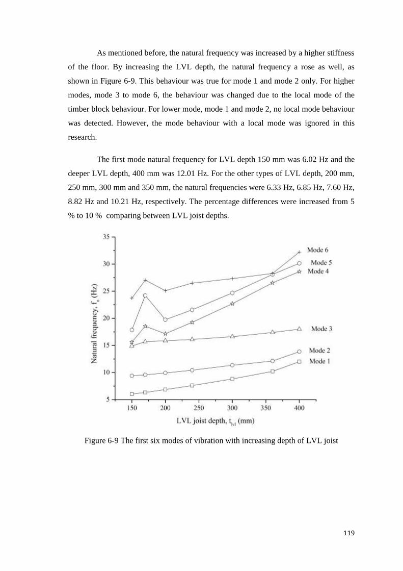
119
As mentioned before, the natural frequency was increased by a higher stiffness
of the floor. By increasing the LVL depth, the natural frequency a rose as well, as
shown in Figure 6-9. This behaviour was true for mode 1 and mode 2 only. For higher
modes, mode 3 to mode 6, the behaviour was changed due to the local mode of the
timber block behaviour. For lower mode, mode 1 and mode 2, no local mode behaviour
was detected. However, the mode behaviour with a local mode was ignored in this
research.
The first mode natural frequency for LVL depth 150 mm was 6.02 Hz and the
deeper LVL depth, 400 mm was 12.01 Hz. For the other types of LVL depth, 200 mm,
250 mm, 300 mm and 350 mm, the natural frequencies were 6.33 Hz, 6.85 Hz, 7.60 Hz,
8.82 Hz and 10.21 Hz, respectively. The percentage differences were increased from 5
% to 10 % comparing between LVL joist depths.
Figure 6-9 The first six modes of vibration with increasing depth of LVL joist
120
6.6 Relationship between concrete topping thickness and LVL joist depth
As shown in Figure 6-10, the vibration behaviour of the LCC floor was
governed mainly by (1) mass and (2) stiffness, for linear elastic response. Furthermore,
the damping ratio, support conditions and human occupancies also gave influences on
the overall floor vibration behaviour. These results described the behaviour of mode 1
only. Figure 6-10 (a) and (b) show that the natural frequencies rose with increasing
thickness of the concrete topping. However, when the LVL joist depth was varied from
150 mm to 200 mm, the behaviour was changed. The natural frequency decreased at the
second point and rose up again at 65 mm of concrete topping thickness. In this case,
vibration of the LCC floor system was governed by mass. This behaviour remained for
the LCC floor with 240 mm and 300 mm depth of LVL joist. Later, for higher LVL
joist depths, the natural frequency reduced at 25 mm to 75 mm of concrete topping
thickness; refer to Figure 6-10 (c) to (e). And then, the natural frequency increased with
the thickness of concrete topping as depicted in Figure 6-10 (f) and (g) when the LCC
floor was dominated by stiffness of the system.
Figure 6-11 shows that the natural frequency generally increased linearly with
the depth of the LVL. However, the differences between the natural frequencies were
smaller when the concrete topping was thicker. This is probably due to the mass of the
concrete which governed the behaviour of the LCC floor compared to the LVL joist. It
indicates that the vibration behaviour of LCC was governed by the mass of the concrete
topping and the stiffness of the LVL joist. For less deep LVL joists, the mass of the
concrete controls the behaviour. But, when the depth of the LVL increased, at some
point, the behaviour was dominated by the stiffness of the LVL. Probably, the
composite action also affects the behaviour before the mass takes over the behaviour
again.
The results from analytical modelling were compared with theoretical
calculations from Eurocode 5 (CEN, 2005) using the formula discussed in Chapter 2.
The percentage difference between the two first mode natural frequencies for an 8 m x
7.8 m LCC floor with varying thickness of concrete topping and LVL joist depth is
depicted in Table 6-2. The results show that the predicted behaviour was similar to the
analytical modelling with the maximum percentage error about 21%. The pattern of the
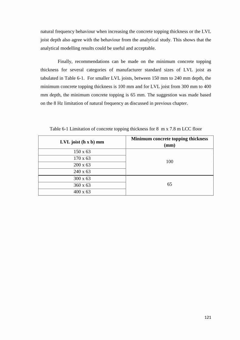
121
natural frequency behaviour when increasing the concrete topping thickness or the LVL
joist depth also agree with the behaviour from the analytical study. This shows that the
analytical modelling results could be useful and acceptable.
Finally, recommendations can be made on the minimum concrete topping
thickness for several categories of manufacturer standard sizes of LVL joist as
tabulated in Table 6-1. For smaller LVL joists, between 150 mm to 240 mm depth, the
minimum concrete topping thickness is 100 mm and for LVL joist from 300 mm to 400
mm depth, the minimum concrete topping is 65 mm. The suggestion was made based
on the 8 Hz limitation of natural frequency as discussed in previous chapter.
Table 6-1 Limitation of concrete topping thickness for 8 m x 7.8 m LCC floor
LVL joist (h x b) mm Minimum concrete topping thickness
(mm)
150 x 63
100 170 x 63
200 x 63
240 x 63
300 x 63
65 360 x 63
400 x 63
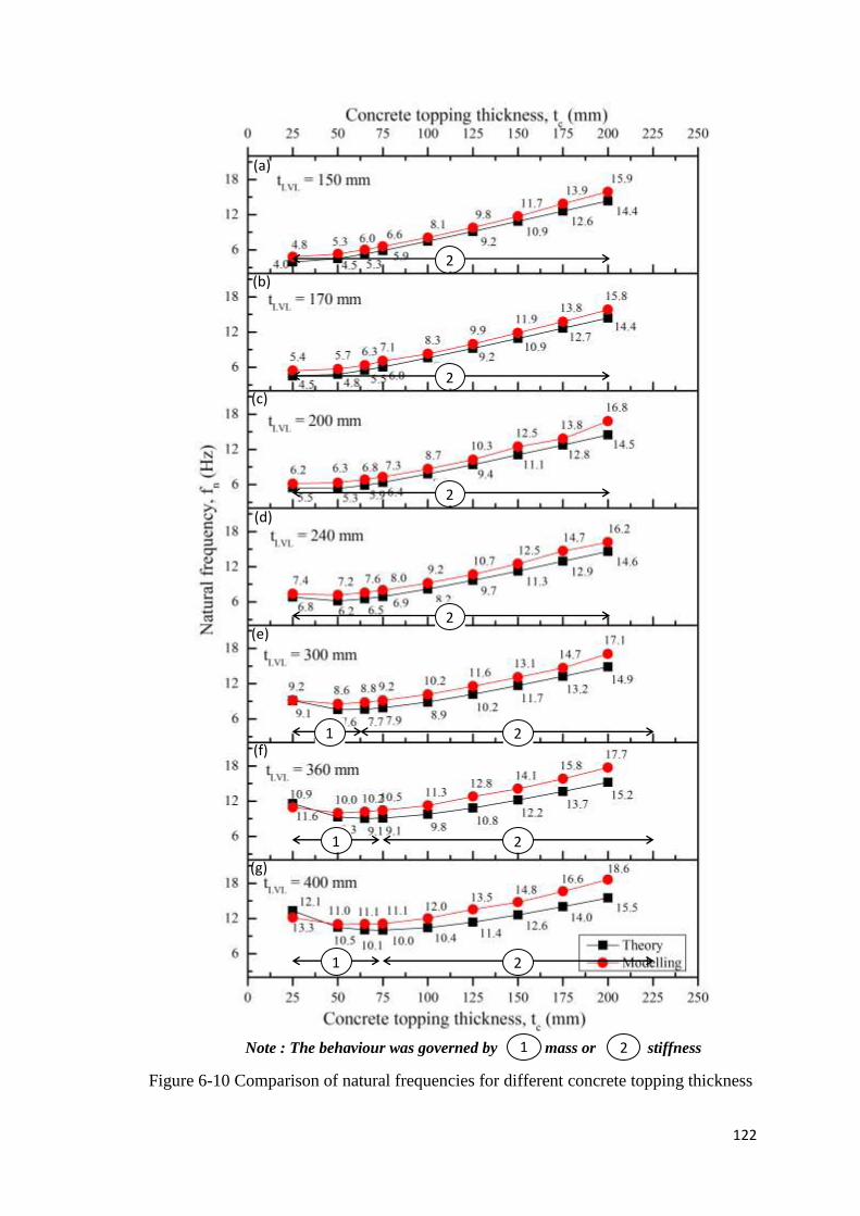
122
Figure 6-10 Comparison of natural frequencies for different concrete topping thickness
1 2
1 2
2
2
2
1 2
2
Note : The behaviour was governed by mass or stiffness 1 2
(a)
(b)
(c)
(d)
(e)
(f)
(g)
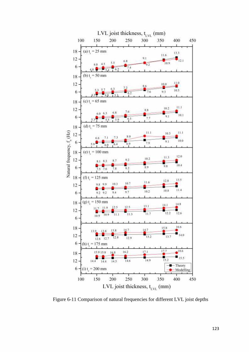
123
Figure 6-11 Comparison of natural frequencies for different LVL joist depths
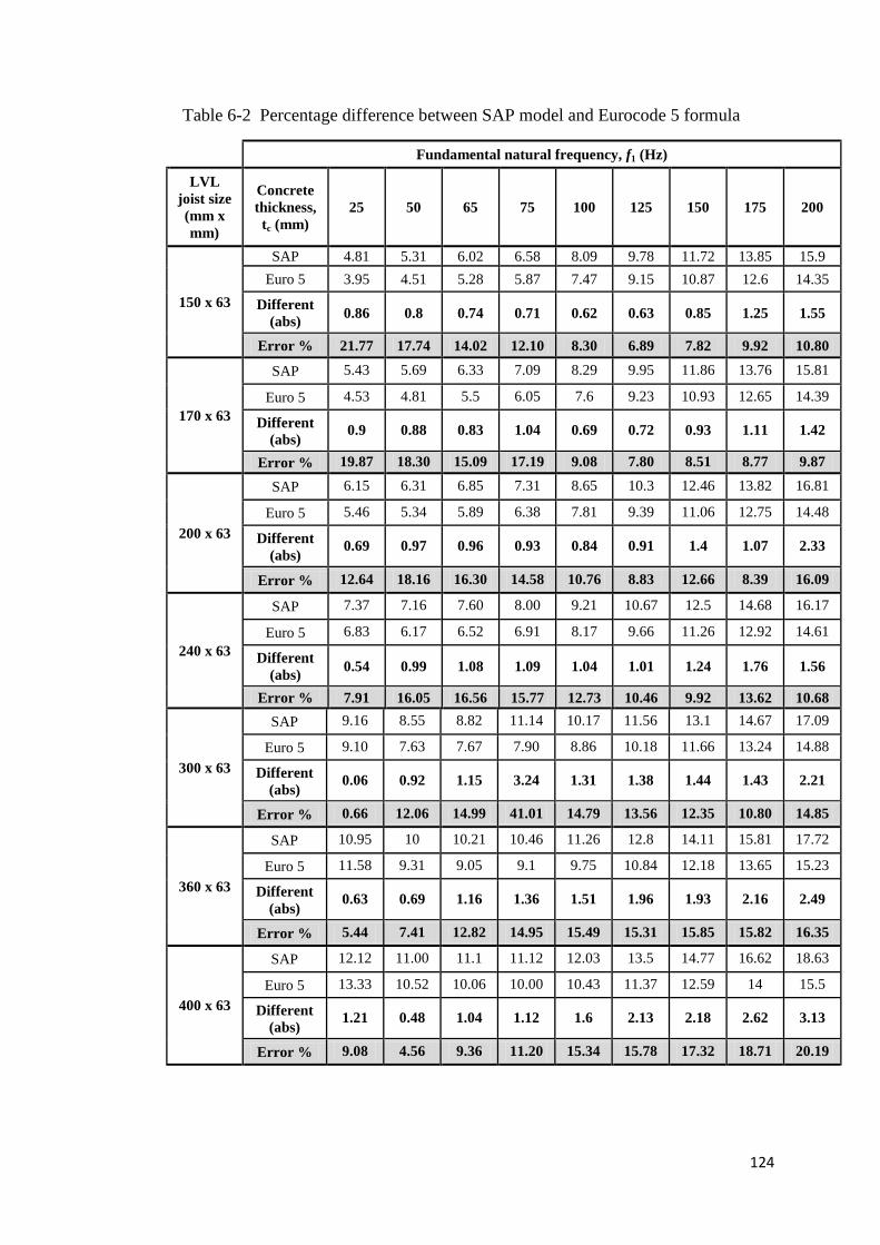
124
Table 6-2 Percentage difference between SAP model and Eurocode 5 formula
Fundamental natural frequency, f1 (Hz)
LVL
joist size
(mm x
mm)
Concrete
thickness,
tc (mm)
25 50 65 75 100 125 150 175 200
150 x 63
SAP 4.81 5.31 6.02 6.58 8.09 9.78 11.72 13.85 15.9
Euro 5 3.95 4.51 5.28 5.87 7.47 9.15 10.87 12.6 14.35
Different
(abs) 0.86 0.8 0.74 0.71 0.62 0.63 0.85 1.25 1.55
Error % 21.77 17.74 14.02 12.10 8.30 6.89 7.82 9.92 10.80
170 x 63
SAP 5.43 5.69 6.33 7.09 8.29 9.95 11.86 13.76 15.81
Euro 5 4.53 4.81 5.5 6.05 7.6 9.23 10.93 12.65 14.39
Different
(abs) 0.9 0.88 0.83 1.04 0.69 0.72 0.93 1.11 1.42
Error % 19.87 18.30 15.09 17.19 9.08 7.80 8.51 8.77 9.87
200 x 63
SAP 6.15 6.31 6.85 7.31 8.65 10.3 12.46 13.82 16.81
Euro 5 5.46 5.34 5.89 6.38 7.81 9.39 11.06 12.75 14.48
Different
(abs) 0.69 0.97 0.96 0.93 0.84 0.91 1.4 1.07 2.33
Error % 12.64 18.16 16.30 14.58 10.76 8.83 12.66 8.39 16.09
240 x 63
SAP 7.37 7.16 7.60 8.00 9.21 10.67 12.5 14.68 16.17
Euro 5 6.83 6.17 6.52 6.91 8.17 9.66 11.26 12.92 14.61
Different
(abs) 0.54 0.99 1.08 1.09 1.04 1.01 1.24 1.76 1.56
Error % 7.91 16.05 16.56 15.77 12.73 10.46 9.92 13.62 10.68
300 x 63
SAP 9.16 8.55 8.82 11.14 10.17 11.56 13.1 14.67 17.09
Euro 5 9.10 7.63 7.67 7.90 8.86 10.18 11.66 13.24 14.88
Different
(abs) 0.06 0.92 1.15 3.24 1.31 1.38 1.44 1.43 2.21
Error % 0.66 12.06 14.99 41.01 14.79 13.56 12.35 10.80 14.85
360 x 63
SAP 10.95 10 10.21 10.46 11.26 12.8 14.11 15.81 17.72
Euro 5 11.58 9.31 9.05 9.1 9.75 10.84 12.18 13.65 15.23
Different
(abs) 0.63 0.69 1.16 1.36 1.51 1.96 1.93 2.16 2.49
Error % 5.44 7.41 12.82 14.95 15.49 15.31 15.85 15.82 16.35
400 x 63
SAP 12.12 11.00 11.1 11.12 12.03 13.5 14.77 16.62 18.63
Euro 5 13.33 10.52 10.06 10.00 10.43 11.37 12.59 14 15.5
Different
(abs) 1.21 0.48 1.04 1.12 1.6 2.13 2.18 2.62 3.13
Error % 9.08 4.56 9.36 11.20 15.34 15.78 17.32 18.71 20.19
125
6.7 Conclusion and Summary
A series of finite element modelling was carried out to analyse and understand
the dynamic behaviour of the LCC flooring system. A few parameters were highlighted
during the analysis including the thickness of concrete topping, the LVL joist depth and
the stiffness of the connectors. As expected and discussed before, the higher stiffness
increased the natural frequency of the system and the higher mass lowered the natural
frequency.
Besides, local mode behaviour was found at the timber block supports, which
reduced the natural frequency of the LCC floor. To reduce the effect of this local mode
behaviour, all edges of the LCC floor should be restrained. However, too many
restraints will increase the stiffness of the LCC floor system and this boundary
condition should applied carefully during the finite element analysis.
During the analysis, the vibration behaviour of the LCC floor was found to be
governed by both stiffness and mass of LVL and concrete topping. When the concrete
topping is increased, the stiffness of the LCC floor also increased due to (i) an increase
in stiffness of the LCC floor with respect to the LVL only beam (which is a positive
effect); and (ii) an increase in mass, due to the weight of the concrete (which is a
negative effect in terms of vibration.
The limitation of concrete topping thickness and LVL joist depth was
proposed in this chapter, especially for 8 m x 7.8 m LCC floor, based on the 8 Hz
limitation of natural frequency. For the deeper LVL joists, from 300 mm to 400 mm
depth, a minimum thickness of 65 mm is suggested. For smaller LVL joists between
150 mm to 240 mm depth, concrete topping with minimum thickness of 100 mm is
recommended.
CHAPTER 7 DESIGN FOR VIBRATION OF LVL- CONCRETE
COMPOSITE (LCC) FLOORS
This chapter presents design guidance to estimate the dynamic behaviour of
long span LCC floors, based on the 8 Hz limitation of fundamental natural frequency,
f1.
7.1 Introduction
The LVL-concrete composite (LCC) floor is one of the solutions for timber
flooring systems. LVL is more flexible than steel and concrete, so the flexibility of the
LVL causes large deflections if LVL is used with traditional timber floors which have
long spans. Associated with this, the resonant frequency of the floor will decrease, and
humans will feel uncomfortable if they can feel the vibration of the floor.
As discussed in Chapter 2, the traditional approach to verify the vibration limit
has been to determine the deflection of the floor under 1 kN point load applied at
midspan, and check that the deflection does not exceed 2 mm. However, due to design
demand nowadays, which requires medium to long spans of floor, the natural
frequency, fn becomes more important. The limitation of fn depends on the stiffness and
mass of the flooring system.
Established standard design procedures (refer section 7.2) give guidance to
estimate the fundamental natural frequency and recommend the limits that should be
satisfied. This chapter provides some recommendation for the designer on the vibration
limitation of long span LCC floors. The guidance includes both an advanced design
method and a simple design method. The equations in the simple design method have
been used to propose the recommended thickness of the concrete topping for different
joist sizes of a LCC floor with a span of 8.0m.
127
7.2 Design criteria
The design criteria have been discussed in detail in Chapter 2 (refer to 2.2.3).
There are no specific requirements to classify floor behaviour exactly as comfortable or
non-comfortable, because the vibration serviceability criterion is very subjective
compared to limit state design for strength or deflection. However, lots of researchers
have recommended a limitation of natural frequency, between 6 Hz to 10 Hz of
fundamental natural frequency (Allen and Murray (1993), Ohlsson (1988), Wyatt
(1989), Smith and Chui (1988), CEN (2004b), Pavic (2009) and Rijal (2013)). Thus, for
this research, the 8 Hz fundamental natural frequency was preferred as a limitation of
vibration serviceability for LCC floors.
7.3 Preliminary design
I. Eurocode static design procedure
The first step in any design will be to estimate the member sizes and the
topping concrete thickness. The static design procedure from Eurocode 5 is
recommended for this purpose.
II. Suggested concrete topping thickness
Suggested values of the minimum concrete topping thickness are proposed
below. The thickness is based on the standard sizes of LVL joists from manufacturers
as illustrated in Table 7-1, but only applicable for 8 m spans. The minimum concrete
topping thickness in Table 7-1 was obtained by using the finite element method in
Section 7.4 and as discussed in Chapter 6. For a floor with a span of 8.0 m and a width
of 7.8m. For LVL joist depth 150 mm to 240 mm with 63 mm breath, the minimum
concrete thickness is 100 mm and for LVL joist depth 300 mm to 400 mm with 63 mm
breath, the minimum concrete thickness is 65 mm. This is as a guide for designer to
estimate the size of LCC floor accordingly to 8 Hz fundamental natural frequency of
vibration serviceability limit. However, for different dimension of floor, the designer
needs to design either by advanced design or simple design method as discussed in
sections 7.4 and 7.5.
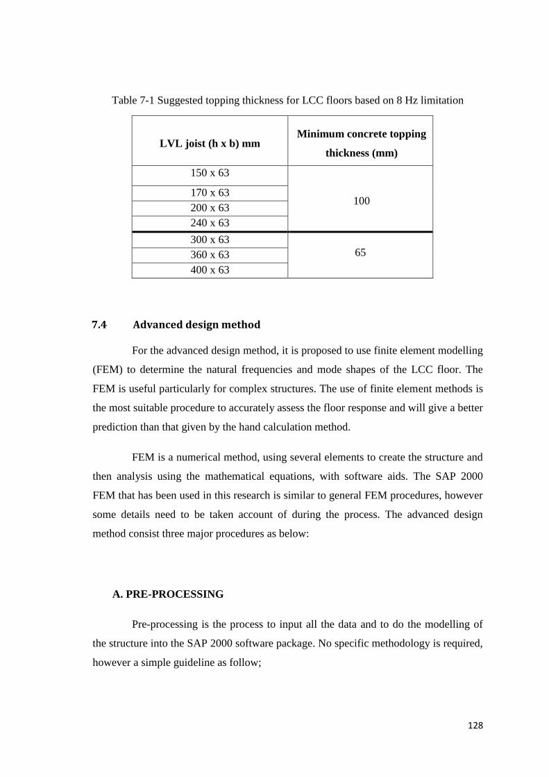
128
Table 7-1 Suggested topping thickness for LCC floors based on 8 Hz limitation
LVL joist (h x b) mm Minimum concrete topping
thickness (mm)
150 x 63
100 170 x 63
200 x 63
240 x 63
300 x 63
65 360 x 63
400 x 63
7.4 Advanced design method
For the advanced design method, it is proposed to use finite element modelling
(FEM) to determine the natural frequencies and mode shapes of the LCC floor. The
FEM is useful particularly for complex structures. The use of finite element methods is
the most suitable procedure to accurately assess the floor response and will give a better
prediction than that given by the hand calculation method.
FEM is a numerical method, using several elements to create the structure and
then analysis using the mathematical equations, with software aids. The SAP 2000
FEM that has been used in this research is similar to general FEM procedures, however
some details need to be taken account of during the process. The advanced design
method consist three major procedures as below:
A. PRE-PROCESSING
Pre-processing is the process to input all the data and to do the modelling of
the structure into the SAP 2000 software package. No specific methodology is required,
however a simple guideline as follow;
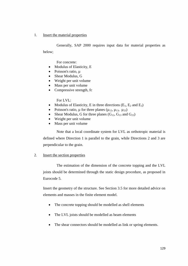
129
1. Insert the material properties
Generally, SAP 2000 requires input data for material properties as
below;
For concrete:
Modulus of Elasticity, E
Poisson's ratio, µ
Shear Modulus, G
Weight per unit volume
Mass per unit volume
Compressive strength, fc
For LVL:
Modulus of Elasticity, E in three directions (E1, E2 and E3)
Poisson's ratio, µ for three planes (µ12, µ13, µ23)
Shear Modulus, G for three planes (G12, G13 and G23)
Weight per unit volume
Mass per unit volume
Note that a local coordinate system for LVL as orthotropic material is
defined where Direction 1 is parallel to the grain, while Directions 2 and 3 are
perpendicular to the grain.
2. Insert the section properties
The estimation of the dimension of the concrete topping and the LVL
joists should be determined through the static design procedure, as proposed in
Eurocode 5.
Insert the geometry of the structure. See Section 3.5 for more detailed advice on
elements and masses in the finite element model.
The concrete topping should be modelled as shell elements
The LVL joists should be modelled as beam elements
The shear connectors should be modelled as link or spring elements.
130
3. Model the structure
After all the properties have been assigned, the next step is model the
structure. See Section 3.5 for more detailed advice. By following the step
described below, the model of the floor can be constructed.
Define the dimensions of the floor. i.e. the span, the width of the floor,
the joist spacing, and number of beams.
Determine the type of shear connection between the LVL joists and the
concrete topping.
Define the boundary conditions including the type of end supports,
edge supports, and the number of continuous spans.
Define the joist hangers or other end supports.
Define a finite element grid and insert finite elements for the joists, the
concrete topping, the shear connectors, and the end supports.
4. Applied load cases
To determine the dynamic floor behaviour, few load cases should be
applied as list below;
Normal design loads for static design
1 kN at mid span for simple estimation of dynamic response
Modal analysis for detailed estimation of dynamic response with Ritz
method.
131
B. PROCESSING
The processing step is carried out by the computer. The computation time will depend
on the complexity of the model.
C. POST- PROCESSING
The results are determine in the post-processing step.
Determine the deflections, natural frequency, mode shape.
Modify the structural sizes or topping thickness as necessary. Re-run
the analysis to get acceptable behaviour.
From the analysis previously described for LCC flooring system, it is clear that
the following parameters and modelling details should be considered.
i. Local axis
The definition of the local axis of each point or member in finite element
modelling is very important to understand especially for applying the
material properties of LVL as an orthotropic material and the stiffness of
the connectors. Wrong interpretation of the local axis will give inaccurate
results.
ii. Local mode behaviour
LVL has lower Young’s Modulus compared to other materials like steel or
concrete, producing higher flexibility. This flexibility of the LVL will
affect the local mode behaviours, especially on the timber beam. Local
mode behaviour will change the behaviour of the LCC system and reduce
the natural frequency. Thus, timber beam should be restrained to increase
the stiffness as well as to avoid the local mode behaviour. Other than that,
each edge support (which is represented as a column) should be assumed
132
as a fixed support to give more accurate results provided that all of the
input variables are assessed correctly.
iii. Mass
The mass of the floor should be input equivalent to the self-weight of the
floor and all other permanent loads that might be present.
iv. Stiffness of multi-span or multi-storey
It is quite complicated to model multi-span or multi-storey TCC floors.
The stiffness of the continuity of the span over the supports or the stiffness
of the structure between adjacent floors should be included. Column
sections should be considered as pinned at both ends.
v. Joist hanger stiffness
The flexibility of joist hangers at the support end of the floor should be
accounted for in the modelling, because the joist hanger flexibility will
affect the floor behaviour. The stiffness should be calculated as described
in Chapter 3.
vi. Mesh
There are no hard and fast rules for the size of the finite elements (or finite
element mesh), but, in general, if the number of elements can be doubled
without significantly changing the frequencies, then there are sufficient
elements and the model should be adopted.
7.5 Simple design method
A simple design method is the easy way to make the first assumptions on the
dynamic behaviour of the floor. By using the basic formulae given below, the
fundamental natural frequency of the LCC floor could be determined.
In many cases the edge condition parallel to the floor joist may be neglected,
and the frequency may be approximated by
( 7-1)
133
where (EI)com is the composite flexural stiffness (Nm2), mcom is the composite
mass per unit length (kg/m) and l is the span length (m).
If the floor system consists of both joists and beams, the fundamental
frequency of the floor system is reasonably well approximated by (Murray et.al, 2003):
( 7-2)
where
fn,floor = fundamental natural frequency of the floor system (Hz),
fn,joist = fundamental natural frequency of the joist alone (Hz),
fn,beam = fundamental natural frequency of the beam supporting the joist (Hz)
Otherwise, to get more accurate result, the fundamental frequency, fn of a LCC
floor system, is calculated from the plate theory by Timoshenko (1964);
(7-3)
where (EI)com is the composite flexural stiffness (Nm2), (EI)x is the stiffness of
floor joists and slab per unit width, (EI)y is the stiffness of floor slab per unit width in a
perpendicular direction to the joists, b is the floor width, mcom is the composite mass per
unit length (kg/m) and l is the span length (m).
The flexural stiffness of the composite beam (EI)com is obtained using the
Equation 7.4, as recommended by Eurocode 5 (CEN, 2004b) and as mentioned in
section 2.1.1;
(7-4)
where (EI)c is the flexural stiffness of concrete topping (Nm2), (EI)t is the
flexural stiffness of LVL joist (N/m2), Ec is the modulus elasticity of concrete topping
134
(N/m2), Et is the modulus elasticity of LVL joist (N/m
2), Ac is the concrete topping area
(m2), At is LVL joist area (m
2).
The ac and at distances can be determined as below:
(7-5a, 7-5b)
Where;
(7-6)
(7-7a, 7-7b)
where seff is the effective spacing (mm) of connection, ks is the slip modulus of
the connection (kN/m), tc is the thickness of concrete topping, tLVL is the thickness of
LVL and tp is the thickness of permanent formwork. The slip modulus was obtained
from the push-out test as discussed in Chapter 2. However, when designing for floor
vibration, the serviceability stiffness should be considered, as the dynamic stiffness of
the floor was found to be 10 % higher than the static stiffness, where the ksls,dynamic = 1.1
x ksls,static.
The effective spacing of connections can be calculated as below
(7-8)
where smin is minimum spacing of connections and smax is maximum spacing of
connections along the beam span.
7.6 Worked Example
The simple design method was applied to a simply-supported LVL-concrete
composite floor spanning 8 m with 400 x 63 mm joists and a 600 x 65 mm concrete
slab. The calculation was evaluated for the walking vibration of a residential or
commercial office floor.
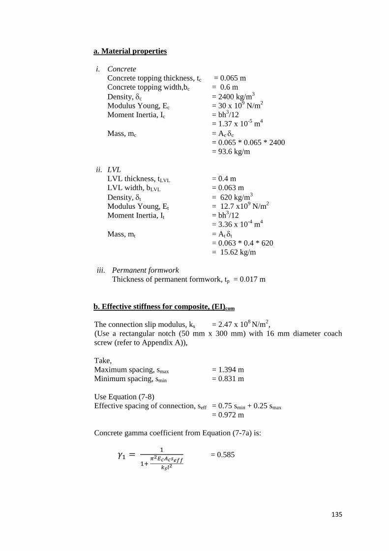
135
a. Material properties
i. Concrete
Concrete topping thickness, tc = 0.065 m
Concrete topping width,bc = 0.6 m
Density, c = 2400 kg/m3
Modulus Young, Ec = 30 x 109 N/m
2
Moment Inertia, Ic = bh3/12
= 1.37 x 10⁻⁵
m4
Mass, mc = Ac c
= 0.065 * 0.065 * 2400
= 93.6 kg/m
ii. LVL
LVL thickness, tLVL = 0.4 m
LVL width, bLVL = 0.063 m
Density, t = 620 kg/m3
Modulus Young, Et = 12.7 x10⁹ N/m
2
Moment Inertia, It = bh3/12
= 3.36 x 10⁻⁴
m4
Mass, mt = At t
= 0.063 * 0.4 * 620
= 15.62 kg/m
iii. Permanent formwork
Thickness of permanent formwork, tp = 0.017 m
b. Effective stiffness for composite, (EI)com
The connection slip modulus, ks = 2.47 x 10⁸ N/m
2,
(Use a rectangular notch (50 mm x 300 mm) with 16 mm diameter coach
screw (refer to Appendix A)),
Take,
Maximum spacing, smax = 1.394 m
Minimum spacing, smin = 0.831 m
Use Equation (7-8)
Effective spacing of connection, seff = 0.75 smin + 0.25 smax
= 0.972 m
Concrete gamma coefficient from Equation (7-7a) is:
= 0.585
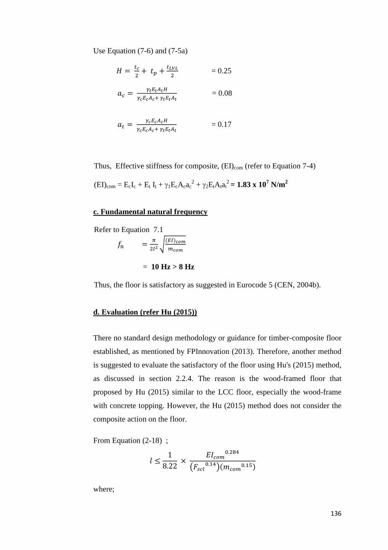
136
Use Equation (7-6) and (7-5a)
= 0.25
= 0.08
= 0.17
Thus, Effective stiffness for composite, (EI)com (refer to Equation 7-4)
(EI)com = EcIc + Et It + 1EcAcac2 + 2EtAtat
2 = 1.83 x 10
7 N/m
2
c. Fundamental natural frequency
Refer to Equation 7.1
= 10 Hz > 8 Hz
Thus, the floor is satisfactory as suggested in Eurocode 5 (CEN, 2004b).
d. Evaluation (refer Hu (2015))
There no standard design methodology or guidance for timber-composite floor
established, as mentioned by FPInnovation (2013). Therefore, another method
is suggested to evaluate the satisfactory of the floor using Hu's (2015) method,
as discussed in section 2.2.4. The reason is the wood-framed floor that
proposed by Hu (2015) similar to the LCC floor, especially the wood-frame
with concrete topping. However, the Hu (2015) method does not consider the
composite action on the floor.
From Equation (2-18) ;
where;
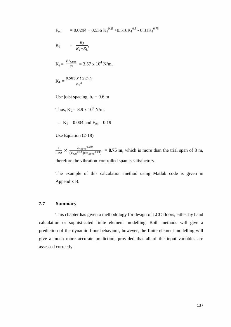
137
Fscl = 0.0294 + 0.536 K10.25
+0.516K10.5
- 0.31K10.75
K1 =
,
Kj =
= 3.57 x 10
4 N/m,
KL =
Use joist spacing, b1 = 0.6 m
Thus, KL= 8.9 x 10⁶ N/m,
K1 = 0.004 and Fscl = 0.19
Use Equation (2-18)
= 8.75 m, which is more than the trial span of 8 m,
therefore the vibration-controlled span is satisfactory.
The example of this calculation method using Matlab code is given in
Appendix B.
7.7 Summary
This chapter has given a methodology for design of LCC floors, either by hand
calculation or sophisticated finite element modelling. Both methods will give a
prediction of the dynamic floor behaviour, however, the finite element modelling will
give a much more accurate prediction, provided that all of the input variables are
assessed correctly.
CHAPTER 8 CONCLUSIONS AND RECOMMENDATIONS FOR
FURTHER WORK
This chapter summarises and concludes the complete work in this research
project. Also, the recommendations for future research, which are mainly findings from
this research, are provided in this chapter.
8.1 Research objectives
The three objectives of this research were given in Chapter 1 as follows:
1. Experimentally characterise the dynamic performance (specifically the natural
frequencies, equivalent viscous damping ratios and mode shapes) of full- and
reduced-scale LVL-concrete composite floor system beams and floors.
2. Implement numerical finite element modelling of the tested structures, full-
and reduced-scale beams and floors, using the results from experimental
modal analysis to verify the models.
3. Propose a simple design method for control of vibration at the serviceability
limit state based on finite element modelling results.
Objectives 1 and 2 have been met fully, as described in the thesis. Objective 3
has been addressed in Chapter 7, and is summarised below.
8.2 Research Summary
The aim of this research was to improve the knowledge of the dynamic
behaviour of LVL-concrete composite (LCC) T-joist flooring system, and to provide
some recommendations to structural engineers to control the vibration of these
structures. To get a better understanding of the vibration behaviour of LCC floors,
experimental modal analysis (EMA) tests and finite element analysis (FEA) were
carried out.
This research began with the experimental modal analysis (EMA) tests on the
6m, 8m and 10m LCC T-joist specimens, to study the vibration behaviour, as discussed
139
in Chapter 3. Then, the experimental works were verified with finite element analysis
(FEA) using the SAP 2000 software package. Both EMA and FEA results show that the
fundamental natural frequencies for 6 m, 8 m and 10 m LCC specimens were 15 Hz, 9
Hz and 6 Hz, respectively. It showed that the 6 m and 8 m LCC specimens were over
the limitation of 8 Hz natural frequency as suggested by Ohlsson (1988) and Eurocode
5 (CEN, 2004b). However, the natural frequency of the 10 m LCC specimens was
under the limitation of 8 Hz natural frequency.
As expected, the longer the specimen, the lower the natural frequency. Thus, it
is suggested that the suitable limitation span length for the tested floor geometry should
not be more than 8 m. In addition, the rigidity of the boundary conditions had a big
influence on the vibration behaviour. Changing the boundary support condition from
flexible (steel roller) to stiffer (timber block) increased the natural frequency of the
floor system, helping to push the natural frequency above 8 Hz.
The experimental results show a general trend for the natural frequencies of
isolated flooring components to decrease when they form part of a larger structural
system, and there is a slight trend for the natural frequencies of the isolated components
to decrease in proportion to the number of similar spans and storeys.
Further research on the effect of topping thickness and LVL joist thickness
was discussed in Chapter 6. The elastic vibration behaviour of the LCC floor was
governed by both stiffness and mass of the LVL and the concrete topping. When the
concrete topping thickness is increased, the stiffness of the LCC floor also increases
due to (i) an increase in stiffness of the LCC floor with respect to the LVL only beam
(which is a positive effect); and (ii) an increase in mass, due to the weight of the
concrete (which is a negative effect in terms of vibration).
The transmission of vibration energy was determined through the multi-span
and multi-storey specimens. With multiple floor systems, the vibration energy was
found to be dissipated and transmitted between spans and storeys. The outer span
received more vibration energy compared to the inner span as illustrated in Chapters 4
and 5. Also, the local mode natural frequency of each span or storey was dominated by
the global mode natural frequency, according to the mode shape behaviour of the
specimens.
140
8.3 Recommendations for designers
1. The recommended design criterion for LCC floors is the widely
accepted limit of 8Hz for the natural frequency of vibration. Floors
with a lower frequency than this will often be unacceptable to users.
2. There is a hierarchy of design methods for assessing the vibration
performance of LCC floors, listed in order of increasing accuracy and
increasing work for the designer:
a. Static deflection of 1mm under a point load of 1kN.
b. Equations for the Simple Design Procedure described in Chapter 7.
c. Detailed finite element analysis, for the Advanced Design
Procedure, as described in Chapter 7.
3. To obtain accurate results, even for simple floors, a finite element analysis
is recommended. However, the input parameters and the modelling
techniques should be considered carefully, as discussed in Chapter 7,
especially for the local mode behaviour.
4. For complex floors that are quite impossible to design by hand, a finite
element analysis is the only way of assessing the vibration frequency of
the floor.
5. The longest practical span for an LCC flooring system such as described
herein, is recommended to be 8m. For spans greater than 8m, the floors
may have an issue with deflections and vibration problems may occur. For
floors spanning more than 8 m, the stiffness would need to be increased by
using bigger joists or a thicker topping, or both. Another possibility would
be to try a reduced joist spacing, or find a way to increase the damping.
6. Designers of some buildings may need to take precautions to ensure that
floor vibrations in one part of the building are not transmitted to other
sections of flooring at the same level, or to floors on other storeys of the
building.
141
8.4 Recommendations for Further Research
1. A methodology has been presented in this thesis for the verification of
analytical models through experimental testing of component parts of real
structures. However, due to the limited time and resources available to this
project, only a small number of structures were actually tested in the
laboratory. Thus, it is recommended that more testing be carried out on full
scale floors in real buildings, so that the vibration behaviour may be
understood better, leading to improved design guidelines.
2. In this research, the effects of adjacent beams on multi-span flooring systems
were investigated using only limited number of tests of a reduced-scale (one-
third scale) 4-span LVL-concrete composite T-joist specimen. It is
recommended that, to increase the confidence of the conclusion drawn in this
thesis, a larger number of tests are required on full-scale TCC flooring
systems, including tests in real buildings.
3. The effect of boundary conditions was partly investigated during the
experimental work. Some end moment fixity was provided by letting the
specimen stand by its own on the laboratory floor. It is recommended that in
future tests, a wider range of support conditions should make sure that there is
no movement at both ends of the specimens during the testing.
4. The propagation of vibration waves was observed during the impact tests on
multi-span LVL-concrete specimens. Future studies should include the effects
of wave propagation in detail, to understand the effect on adjacent beams and
on other floors, where the vibration energy is transmitted between floors.
5. Finite Element Analysis was applied to all the tested LVL-concrete composite
specimens and multi-span LVL-concrete composite specimens. For realistic
floors, the FEA was only applied to one typical floor. Hence, it is
recommended that the FEA should be applied to a much wider range of full-
scale LVL-concrete composite flooring systems.
6. There should be more experimental study of the vibration criteria for a floor
subject to human walking excitation, including the effects of damping.
142
REFERENCES
Abd Ghafar, N. H, (2008). Forced vibration testing on LVL-concrete composite floor system,
7th
Fib Phd Symposium in Stuttgart, Germany, pp. 1-6.
Abd Ghafar, N.H., Deam, B., Fragiacomo, M. & Buchanan, A. (2008). Vibration
performance of LVL-concrete conposite floor systems. 10th
World Conference on
Timber Engineering WCTE, vol. CD. Miyazaki, Japan.
Abd Ghafar N H, Deam, B., Fragiacomo, M., Buchanan, A. (2008). Susceptibility to
Vibrations of LVL-Concrete Composite Floors. Workshop Italiano Sulie Composite.
Benevento, Ilaty: University Degli Studi Del Sannio.
Allen, D. E., & Murray, T. M. (1993). Design criterion for vibrations due to walking.
Engineering Journal, 30(4), 117–129.
ARUP (2012). Technical Report on Nelson Marlborough Institute of Technology Arts and
Media Building - Vibration and Acoustic Study, Opus, Australia.
AS/NZS, (2002). AS/NZS 1170.0:2002 Structural design actions. Part 0: General Principles.
Sydney and Wellington (Jointly publish).
Bachmann, H. & Ammann, W. ,(1987). Vibrations in Structures: Induced by Man and
Machines, IABSE-AIPCIVBH, Zurich, Switzerland.
Bernard, E. S. (2008). Dynamic Serviceability in Lightweight Engineered Timber Floors.
Journal of Structural Engineering, 134(2), 258–268.
Bernard, S. (2003). Vibration of composite timber and concrete flooring. Victoria, Australia:
Forest & Wood Products Reseach & Development Corporation.
Benitez, M.F. (2000). Development and testing of timber/concrete shear connector.
Proceddings of the World Conference on Timber Eingineering 2000. Vancauver, BC,
Canada, paper 8.3.2
Blakeborough, A., & Williams, M. S. (2003). Measurement of floor vibrations using a heel
drop test. Proceedings of the Institution of Civil Engineers: Structures and Buildings,
156(4), 367-371.
Brunner, M., Romer, M., & Schnuriger, M. (2007). Timber-concrete-composite with an
adhesive connector (wet on wet process). Materials and Structures/Materiaux et
Constructions, 40(1), 119–126.
Canadian Construction Materials Centre (CCMC), (1997). Development of Design
Procedures for Vibration Controlled Spans using Engineered Wood Members. Canadian
Wood Council, DMO associates, Quaile Engineering Ltd., Forintek Canada Corp.
Ottawa.
Ceccotti, A. (1995). Timber-Concrete Composite Structures. Timber Engineering, Step 2 (1st
Edition). Centrum Hout, The Netherlands.
143
Ceccotti, A. (2002). Composite concrete-timber structures. Progress in Structural
Engineering and Materials, 4(3), 264–275.
CEN (2004b). Design of timber structures. In Part 1-1: General rules and rules for buildings.
Brussels, Belgium.
Crocetti, R, Sartori, T & Flansbjer, M. (2010). Timber-Concrete Composite Structures with
Prefabricated FRC Slab, World Conference on Timber Engineering, Italy.
Crocetti, R, Sartori, T & Tomasi, R (2015). Innovative Timber-Concrete Composite
Structures with Prefabricated FRF Slabs, Journal of Structural Engineering, 141(9), 1-
10
Deam B, Fragiacomo M, Gross LS (2008). Experimental behaviour of prestressed
LVLconcrete composite beams. Journal of Structural Engineering - ASCE. 134(5), 801-
809.
Devine, P.J, Smith, A.L. & Hicks, S.J (2007). Design Guide on the Vibration Floors (2nd
Edition). The Steel Construction Institute (SCI). Berkshire, United Kindom
Dolan, J. D. et al. (1999). Preventing Annoying Wood Floor Vibrations. Journal of Structural
Engineering,Vol.125 (1), 19-24.
Ebrahimpour, A et. al, (1996). Measuring and Modeling Dynamic Loads Imposed by
Moving Crowds. Journal of Structural Engineering, 122(12), 1468–1474.
Ebrahimpour, A., & Sack, R. L. (1989). Modeling Dynamic Occupant Loads. Journal of
Structural Engineering, 115(6), 1476–1496.
Ebrahimpour, A., & Sack, R. L. (1992). Design Live Loads for Coherent Crowd Harmonic
Movements. Journal of Structural Engineering, 118(4), 1121–1136.
El-Dardiry, E., & Ji, T. (2006). Modelling of the dynamic behaviour of profiled composite
floors. Engineering Structures, 28(4), 567–579.
Ellingwood, A. & Tallin, B. (1984). Structural serviceability: floor vibrations. Journal of
Structural Engineering, 110(2), 410–419.
Franklin K & Hough R., (2014). Modelling and measurement of the dynamic performance of
a timber concrete composite floor. In Wood Engineering Conforence (p. CD). Quebec
City, Canada.
Fuller, A. H. (1924). Dynamic effects of moving floor loads - stresses measured in the floor
and balcony of a college gymnasium. Am Arch Arch, 126(11), 455–456.
FPInnovations (2013). Technical Guide for the Design and Construction of Tall Wood
Building in Canada. Quebec.
Gross, S. L. (2004). Experimental testing on prestressed timber-concrete composite beams.
Civil Engineering. University of Canterbury, New Zealand.
144
Gutkowski, R, Balogh, J., Natterer, Brown, K., Koike, E. &Etournaud, P, (2000). Laboratory
tests of composite wood-concrete beam and floor specimens. Sixth World Conference on
Timber Engineering. Whistler.
Hehhl, S., Tannert. T., Meena, R. and Vallee, T., (2014). Experimental and Numerical
Investigations of Groove Connections for a Novel Timber-Concrete Composite System.
Journal of Performance of Constructed Facilities, 28(6), A4014010
Hu, L.J., (2007). Design Guide for Wood-framed Floor Systems. Canadian Forest Service
Report N0. 32. Quebec:FPInnovations.
Hu, L. J., (2015). Mid-rise Wood-Frame Construction Handbook, First Edition,
FPInnovations, Quebeq.
ISO (1989). ISO 2631-2:1989 evaluation of human exposure to whole-body
vibration - part 2: Continuous and shock-induced vibration in buildings (1 to 80Hz).
Lenzen, K. H. (1966). Vibration of steel joist-concrete slab floors. American Institute of Steel
Construction -- Engineering Journal, 3(3), 133–136.
Ljunggren, F., (2006). Floor Vibration - Dynamic Properties and Subjective Perception,
Lulea University of Technology, Sweden.
Mertens, C., Martin, Y., & Dobbels, F. 2007. Investigation of the vibration behaviour of
Timber-Concrete composite floors as part of a performance evaluation for the Belgian
building industry. Building Acoustics, 14 (1), 25-36.
Murray, T.M, Allen, D.E. & Ungar, E.E., (2003). Floor Vibration due to Human Activity.
United States of America: American Institute of Steel Construction.
Natterer, J., Hamm, J., & Favre, P., (1996). Composite wood-concrete floors for
multistorey buildings. In Wood Engineering Conforence (Vol. 3, pp. 3425–3431).
Omnipress, Madison, Wls.
National Research Council (NRC), (2010). National Building Coe of Canada (NBC).
National Research Council of Canada, Ottawa.
Nauta, F. (1970). Composite Glulam beam-reinforced concrete deck bridges. Test report 364,
Central labs.
Nelson, F. C. (1974). Subjective rating of building floor vibration. Sound and Vibration, 8,
34–37.
Nguyen, T., Gad, E., Wilson, J. & Haritos, N.,( 2012). Improving a current method for
predicting walking-induced floor vibration , Steel and Composite Structures, 13 (2), pp 139-
155.
Nguyen, T., Gad, E., Wilson, J. & Haritos, N. (2014). Mitigating foot fall induced
vibration in long-span floors, Australian Journal of Structural Engineering, 15(1), pp.
97-109,
145
Ohlsson, S (1988). Springiness and human-indiced floor vibrations – A design guide.Swedish
Council for Bulding Research , Stockholm, Sweden
Pavic, A., & Reynolds, P. (2003). Modal testing and dynamic FE model correlation and
updating of a prototype high-strength concrete floor. Cement and Concrete Composites,
25(7), 787–799.
Pavic, A., Widjaja, T., & Reynolds, P. (2002). The use of modal testing and FE model
updating to investigate vibration transmission between two nominally identical building
floors. In International Conference on Structure Dynamics Modeling–Test, Analysis,
Correlation and Validation (pp. 347-355).
Pernica, G., & Allen, D.E, (1982). Floor vibration measurements in a shopping centre.
Canadian Journal of Civil Engineering, 9(2), 149.
Rainer, J. H. (1980). Dynamic tests on a steel-josit concrete-slab floor. Canadian Journal of
Civil Engineering, 7(2), 213–224.
Reiher, H., & Meister, F. (1931). The effect of vibration on people. Forschung Im
Ingenieurwesen, 2(11), 381–386 (in German). Retrieved from
Reynolds, P., Pavic,A. (2000). Quality Assurance Procedures for the Modal Testing of
Building Floor Structures. Experimental Techniques, 24(4), 36-41.
Rijal, R., Samali, B. & Crews, K. (2010). Dynamic performance of the timber-concrete
composite flooring systems, Australasian Conference on the Mechanics of Structures
and Materials (ACMSM) 21, Melbourne, Australia.
Rijal, R. (2013). Dynamic performance of timber and timber-concrete composite flooring
systems. University of Technology, Sydney.
SAP2000. (1997). User Manual : Integrated Finite Element Analysis and Design Structures:
Computer and Structures, Inc.
Seibold, E. (2004). Feasibility study for composite concrete-timber floor systems using
laminated veneer lumber in New Zealand. University of Karlsruhe, Germany.
Setareh, M. & Hanson, R. (1992). Tuned mass dampers for balcony vibration control.
Journal of Structural Engineering – ASCE, 118( 3), pp. 723-740.
Skinner J. M. (2013). Thin topping timber-concrete composite floors. University of Bath.
Skinner J., Harris R., Paine K., Walker P., and B. J. (2013). Ultra-thin topping upgrades for
improved serviceability performance. Advanced Materials Research, (778), 673–681.
Smith, I. and Chui, Y. H., (1988). Design of lightweight wooden floors to avoid human
discomfort. Canadian Journal of Engineering, 15(2), 254-262.
Soltis L.A. & Hunt M.O, (2002). Vibration testing of timber floor systems. Forest Products
Journal, 52(10), 75–81.
146
Stojić, D., & Cvetković, R. (2001). Analysis of a composite tim-ber-concrete structures
according to the limit states de-sign and innovative methods in coupling of a timber and
concrete . Facta Universitatis Series: Architecture and Civil Engineering , v.2(No3 ),
p.169–184.
Thornton, C. H., Cuoco, D. A. & Velivasakis, E.E.( 1990), “Taming Structural Vibrations”,
Civil Engineering – ASCE, Vol. 60, No. 11, pp. 57-59.
Timoshenko, S. (1964). Theory of Plates and Shells. London:McGraw-Hill , 2nd ed.
Tilden, C. J. (1913). Kinetic effects of crowds. Proceedings of the American Society of Civil
Engineers, 34(3), 325-340.
Tuan, C. Y., & Saul, W. E. (1985). Loads due to spectator movements. Journal of Structural
Engineering, 111(2), 418–434.
Ungar, E. E. (1978). Footfall-induced vibrations of floors supporting sensitive equipment.
The Journal of the Acoustical Society of America, 64(S1), S26-S26
Van der Linden, M. L. R. (1999). Timber-Concrete Composite Floor Systems . TU Delft,
Delft University of Technology .
Webster, A. & Vaicaitis, R. 1992, “Application of tuned mass dampers to control vibrations
of composite floor systems”, Engineering Journal of the American Institute of Steel
Construction, 29( )3, pp. 116-124.
Wiss, J. F., & Parmelee, R. A. (1974). Human perception of transient vibrations. American
Institute of Steel Construction, 100(4), 773–787.
Wyatt, T. A. (1989). Design Guide on The Vibration of Floors (SCI Publication 076). Ascot,
UK: SCI.
Yeoh Fragiacomo, M., Abd. Ghafar, N.H, Buchanan, A., Deam, B., D. (2008). Behaviour of
timber-concrete composite floor systems. Australasian Structural Engineering
Conference. Melbourne, Australia.
Yeoh, D. (2010). Behaviour and design of timber-concrete composite floor system.
University of Canterbury, New Zealand.
Zivanovic, S., & Pavic, A. (2009). Probabilistic Modeling of Walking Excitation for Building
Floors. Journal of Performance of Constructed Facilities, 23(3), 132–143.
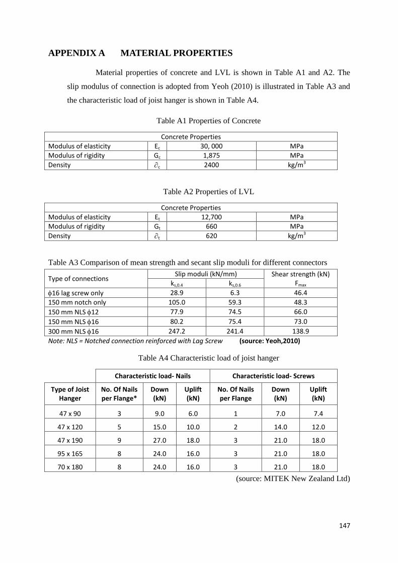
147
APPENDIX A MATERIAL PROPERTIES
Material properties of concrete and LVL is shown in Table A1 and A2. The
slip modulus of connection is adopted from Yeoh (2010) is illustrated in Table A3 and
the characteristic load of joist hanger is shown in Table A4.
Table A1 Properties of Concrete
Concrete Properties
Modulus of elasticity Ec 30, 000 MPa
Modulus of rigidity Gc 1,875 MPa
Density c 2400 kg/m3
Table A2 Properties of LVL
Concrete Properties
Modulus of elasticity Et 12,700 MPa
Modulus of rigidity Gt 660 MPa
Density t 620 kg/m3
Table A3 Comparison of mean strength and secant slip moduli for different connectors
Type of connections Slip moduli (kN/mm) Shear strength (kN)
Fmax ks,0.4 ks,0.6
16 lag screw only 28.9 6.3 46.4
150 mm notch only 105.0 59.3 48.3
150 mm NLS 12 77.9 74.5 66.0
150 mm NLS 16 80.2 75.4 73.0
300 mm NLS 16 247.2 241.4 138.9
Note: NLS = Notched connection reinforced with Lag Screw (source: Yeoh,2010)
Table A4 Characteristic load of joist hanger
Characteristic load- Nails Characteristic load- Screws
Type of Joist Hanger
No. Of Nails per Flange*
Down (kN)
Uplift (kN)
No. Of Nails per Flange
Down (kN)
Uplift (kN)
47 x 90 3 9.0 6.0 1 7.0 7.4
47 x 120 5 15.0 10.0 2 14.0 12.0
47 x 190 9 27.0 18.0 3 21.0 18.0
95 x 165 8 24.0 16.0 3 21.0 18.0
70 x 180 8 24.0 16.0 3 21.0 18.0
(source: MITEK New Zealand Ltd)
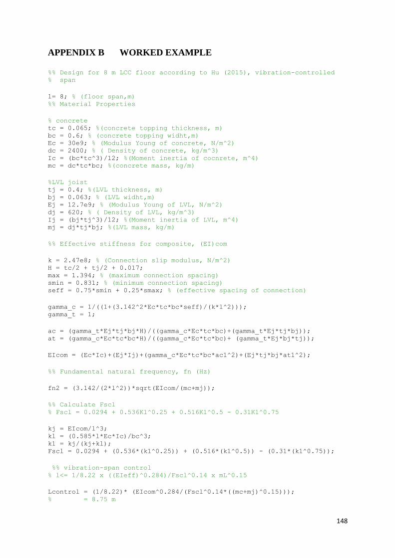
148
APPENDIX B WORKED EXAMPLE
%% Design for 8 m LCC floor according to Hu (2015), vibration-controlled % span
l= 8; % (floor span,m) %% Material Properties
% concrete tc = 0.065; %(concrete topping thickness, m) bc = 0.6; % (concrete topping widht,m) Ec = 30e9; % (Modulus Young of concrete, N/m^2) dc = 2400; % ( Density of concrete, kg/m^3) Ic = (bc*tc^3)/12; %(Moment inertia of cocnrete, m^4) mc = dc*tc*bc; %(concrete mass, kg/m)
%LVL joist tj = 0.4; %(LVL thickness, m) bj = 0.063; % (LVL widht,m) Ej = 12.7e9; % (Modulus Young of LVL, N/m^2) dj = 620; % ( Density of LVL, kg/m^3) Ij = (bj*tj^3)/12; %(Moment inertia of LVL, m^4) mj = dj*tj*bj; %(LVL mass, kg/m)
%% Effective stiffness for composite, (EI)com
k = 2.47e8; % (Connection slip modulus, N/m^2) H = tc/2 + tj/2 + 0.017; max = 1.394; % (maximum connection spacing) smin = 0.831; % (minimum connection spacing) seff = 0.75*smin + 0.25*smax; % (effective spacing of connection)
gamma_c = 1/((1+(3.142^2*Ec*tc*bc*seff)/(k*l^2))); gamma_t = 1;
ac = (gamma_t*Ej*tj*bj*H)/((gamma_c*Ec*tc*bc)+(gamma_t*Ej*tj*bj)); at = (gamma_c*Ec*tc*bc*H)/((gamma_c*Ec*tc*bc)+ (gamma_t*Ej*bj*tj));
EIcom = (Ec*Ic)+(Ej*Ij)+(gamma_c*Ec*tc*bc*ac1^2)+(Ej*tj*bj*at1^2);
%% Fundamental natural frequency, fn (Hz)
fn2 = (3.142/(2*l^2))*sqrt(EIcom/(mc+mj));
%% Calculate Fscl % Fscl = 0.0294 + 0.536K1^0.25 + 0.516K1^0.5 - 0.31K1^0.75
kj = EIcom/l^3; kl = (0.585*l*Ec*Ic)/bc^3; k1 = kj/(kj+kl); Fscl = 0.0294 + (0.536*(k1^0.25)) + (0.516*(k1^0.5)) - (0.31*(k1^0.75));
%% vibration-span control % l<= 1/8.22 x ((EIeff)^0.284)/Fscl^0.14 x mL^0.15
Lcontrol = (1/8.22)* (EIcom^0.284/(Fscl^0.14*((mc+mj)^0.15))); % = 8.75 m

149
% The required span, 8 m less than the vibration-controlled span, 8.75 m, % Thus, the design can be accepted.
Recommended