ABSTRACT
Title of dissertation: The Optical Response of Strongly CoupledQuantum Dot- Metal NanoparticleHybrid Systems
Ryan Domenick Artuso, Doctor of Philosophy, 2012
Dissertation directed by: Dr. Garnett W. BryantNational Institute of Standards and Technology
In this thesis, we study, theoretically, hybrid systems composed of semicon-
ducting quantum dots (SQDs) and metallic nanoparticles (MNPs) which are coupled
by means of an applied optical field. Systems composed of SQDs and MNPs have
recently been a very active area of research. Such structures are considered to be
viable candidates for use in nanodevices in quantum information and nanoscale ex-
citation transfer. The goal of this thesis is to investigate the interactions of the
constituent particles and predict the hybrid response of SQD/MNP systems.
We first study a single SQD coupled to a spherical MNP, and explore the
relationship between the size of the constituents and the response of the system.
We identify four distinct regimes of behavior in the strong field limit that each
exhibit novel properties, namely, the Fano regime, exciton induced transparency,
suppression and bistability. In chapter 3, we will explore these four regimes in
detail and set bounds on each.
In chapter 4, we then show that the response of the system can be tailored by

engineering metal nanoparticle shape and the exciton resonance of SQDs to control
the local-fields that couple the MNPs and SQDs. We identify regimes where dark
modes and higher order multipolar modes can influence hybrid response. Exter-
nal fields do not directly drive MNP dark modes, so SQD/MNP coupling is dom-
inated by the local induced coupling, providing a situation in which the induced
self-interaction could be probed using near field techniques.
Finally, we consider a system of two SQDs coupled to a MNP. In particular, we
identify and address issues in modeling the system using a semiclassical approach,
which can lead to unstable and chaotic behavior in a strong SQD-SQD coupling
regime. When we model the system using a more quantum mechanical approach,
this chaotic regime is absent. Finally, we compare the two models on a system
with a strong plasmon-mediated interaction between the SQDs and a weak direct
interaction between them.

The Optical Response of Strongly Coupled
Quantum Dot- Metal NanoparticleHybrid Systems
by
Ryan Domenick Artuso
Dissertation submitted to the Faculty of the Graduate School of theUniversity of Maryland, College Park in partial fulfillment
of the requirements for the degree ofDoctor of Philosophy
2012
Advisory Committee:Doctor Garnett W. Bryant, AdvisorProfessor Christopher J. Lobb, ChairDoctor Eite TiesingaProfessor Mario DagenaisProfessor Jeremy N. Munday

c© Copyright by
Ryan Domenick Artuso2012

Acknowledgments
I would like to thank my advisor Garnett Bryant for his guidance and support,
and for the opportunities he has given me. I would also like to thank the committee
members for taking time from their busy schedules to read and review my work, and
for their invaluable feedback. I’d also like to acknowledge our collaborators Javier
Aizpurua and Aitzol Garcia-Etxarri for their help and excellent discussions. Finally,
I’d like to thank Sarah Roosa for all her help, support, and encouragement.
ii
Table of Contents
List of Figures v
1 Background and Motivation 11.1 Introduction . . . . . . . . . . . . . . . . . . . . . . . . . . . . . . . . 11.2 Nanoparticles . . . . . . . . . . . . . . . . . . . . . . . . . . . . . . . 31.3 Nanosuperstructures . . . . . . . . . . . . . . . . . . . . . . . . . . . 51.4 Transmission of Quantum Information . . . . . . . . . . . . . . . . . 7
2 Tools and Toys 102.1 Metallic Nanoparticles . . . . . . . . . . . . . . . . . . . . . . . . . . 11
2.1.1 Modeling the MNP response to a planewave . . . . . . . . . . 132.1.2 The Drude Model . . . . . . . . . . . . . . . . . . . . . . . . . 182.1.3 Numerical Methods . . . . . . . . . . . . . . . . . . . . . . . . 202.1.4 Modeling the MNP Response to a Dipole Source . . . . . . . . 22
2.2 Semiconducting Quantum Dots . . . . . . . . . . . . . . . . . . . . . 232.3 Quantum Open Systems . . . . . . . . . . . . . . . . . . . . . . . . . 252.4 The Density Matrix . . . . . . . . . . . . . . . . . . . . . . . . . . . . 282.5 The Interaction of Light and Matter . . . . . . . . . . . . . . . . . . 302.6 Stimulated and Spontaneous Emission . . . . . . . . . . . . . . . . . 362.7 Toy Model: Two Level System Interacting with a Single Bosonic Mode 402.8 Lindblad Master Equation . . . . . . . . . . . . . . . . . . . . . . . . 442.9 The Interaction of Light and Matter: Revisited . . . . . . . . . . . . 512.10 Computational Technique . . . . . . . . . . . . . . . . . . . . . . . . 56
3 The Optical Response of Strongly Coupled SQD-MNP Systems 573.1 Introduction . . . . . . . . . . . . . . . . . . . . . . . . . . . . . . . . 583.2 Setup . . . . . . . . . . . . . . . . . . . . . . . . . . . . . . . . . . . . 61
3.2.1 Energy . . . . . . . . . . . . . . . . . . . . . . . . . . . . . . . 663.2.2 Numerical Calculations and Parameter Values . . . . . . . . . 68
3.3 Region I: Nonlinear Fano Effect . . . . . . . . . . . . . . . . . . . . . 703.4 Region II: Exciton Induced Transparency (EXIT) . . . . . . . . . . . 713.5 Transition Region: Suppression . . . . . . . . . . . . . . . . . . . . . 743.6 Region III: Bistability . . . . . . . . . . . . . . . . . . . . . . . . . . 79
3.6.0.1 Analysis of Initial Conditions . . . . . . . . . . . . . 833.6.1 Calculation of the Resonance Shift . . . . . . . . . . . . . . . 84
3.7 Running (the) Interference: Phasors and Interaction Strengths . . . . 873.7.1 The Phase Change of ρ12 . . . . . . . . . . . . . . . . . . . . . 89
3.8 The Effect of Polarization . . . . . . . . . . . . . . . . . . . . . . . . 923.9 A Summary of Findings . . . . . . . . . . . . . . . . . . . . . . . . . 94
iii
4 Engineered SQD-MNP Systems with Extended Geometries 974.1 Introduction . . . . . . . . . . . . . . . . . . . . . . . . . . . . . . . . 974.2 Setup . . . . . . . . . . . . . . . . . . . . . . . . . . . . . . . . . . . . 100
4.2.1 System Energy . . . . . . . . . . . . . . . . . . . . . . . . . . 1044.2.2 Numerical Calculations in the Large Field Limit . . . . . . . . 105
4.3 Advantages of Using a Full Electrodynamical Description . . . . . . . 1064.3.1 Comparison Between a Full Electrodynamical Calculation and
a Non-Retarded Multipole Expansion for Spherical MNPs . . 1074.3.2 From Spheres to Rods . . . . . . . . . . . . . . . . . . . . . . 110
4.3.2.1 Coupling to Dark States vs. Bright States . . . . . . 1124.4 Engineered Systems . . . . . . . . . . . . . . . . . . . . . . . . . . . . 113
4.4.1 Dynamics of a 70 nm Nanorod . . . . . . . . . . . . . . . . . . 1154.4.2 Exciton Induced Transparency in the non-Retarded Limit . . . 119
4.5 Concluding Remarks . . . . . . . . . . . . . . . . . . . . . . . . . . . 122
5 Multiple SQD Systems 1235.1 Introduction . . . . . . . . . . . . . . . . . . . . . . . . . . . . . . . . 1245.2 SQD-MNP-SQD Hybrid Molecule . . . . . . . . . . . . . . . . . . . . 126
5.2.1 The SQD-SQD Interaction . . . . . . . . . . . . . . . . . . . . 1295.2.2 Numerical Calculations . . . . . . . . . . . . . . . . . . . . . . 130
5.3 Semiclassical Approach to SQD-SQD coupling . . . . . . . . . . . . . 1315.3.1 Weak Field Limit . . . . . . . . . . . . . . . . . . . . . . . . . 1335.3.2 Strong Field Limit: a vs. µ Parameter Space . . . . . . . . . . 1355.3.3 Transition: Chaotic Solutions . . . . . . . . . . . . . . . . . . 138
5.3.3.1 Explicit Symmetry Breaking . . . . . . . . . . . . . . 1395.3.3.2 The symmetric-antisymmetric basis . . . . . . . . . . 143
5.4 Towards A More Quantum Mechanical Approach . . . . . . . . . . . 1485.4.1 Quantum Mechanical SQD-SQD Coupling . . . . . . . . . . . 1495.4.2 Numerical Results . . . . . . . . . . . . . . . . . . . . . . . . 1515.4.3 Dipole Blockade . . . . . . . . . . . . . . . . . . . . . . . . . . 1535.4.4 Comparison in the Weak SQD-SQD Coupling Regime . . . . . 155
5.5 Conclusions . . . . . . . . . . . . . . . . . . . . . . . . . . . . . . . . 157
6 Concluding Remarks 1606.1 Looking Ahead . . . . . . . . . . . . . . . . . . . . . . . . . . . . . . 163
Bibliography 165
iv
List of Figures
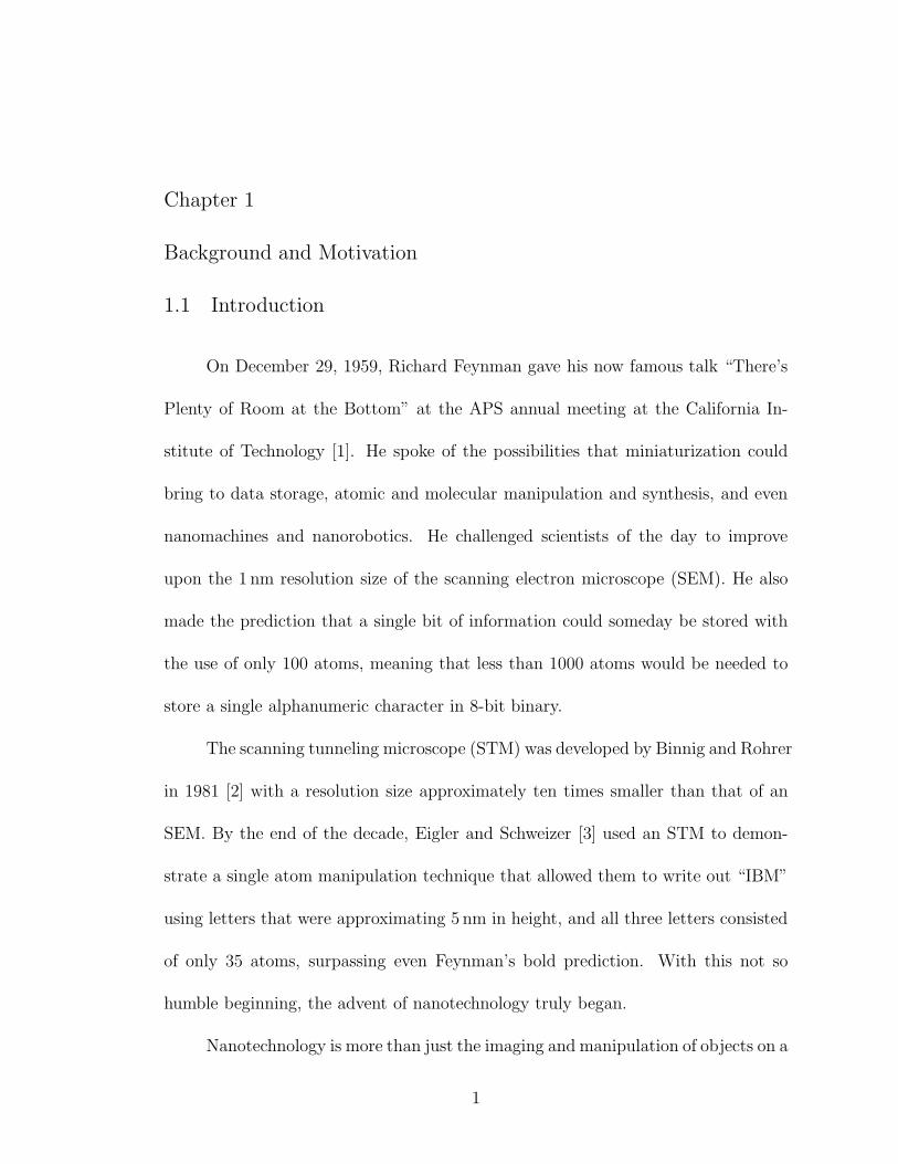
1.1 An artist’s rendition of a C60 buckminsterfullerene. Each of the black dots rep-
resents a single carbon atom. Graphic generated using Mathematica software. . 2
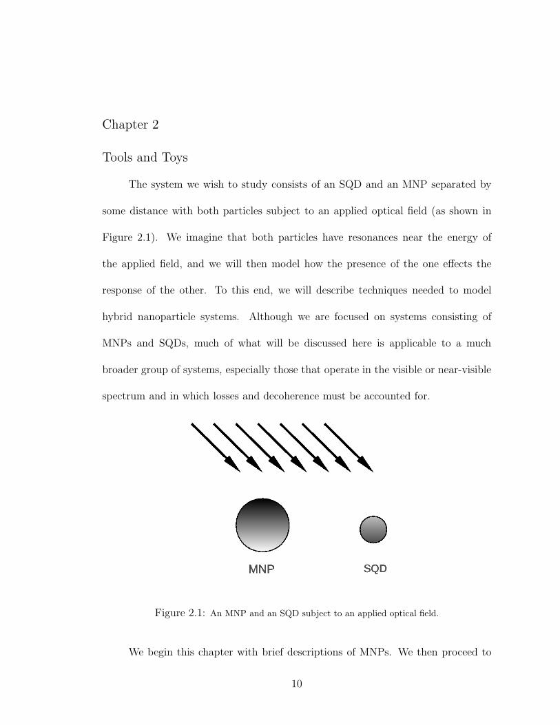
2.1 An MNP and an SQD subject to an applied optical field. . . . . . . . . . . . . 102.2 Spherical MNP in an applied driving field. . . . . . . . . . . . . . . . . . . . 132.3 The magnitude (solid line), the real part (dotted line) and the imaginary part
(dashed line) of ǫ0ǫDrude
plotted as a function of ωωp
with Γ 0.1ωp. The plasmon
peak (the peak in the magnitude of ǫ0ǫDrude
) appears at a dip in the imaginary part
at ωωp
1, where the real part crosses zero. . . . . . . . . . . . . . . . . . . 182.4 The magnitude (solid line), the real part (dotted line) and the imaginary part
(dashed line) of ǫ0ǫeff
plotted as a function of ωωp
with Γ 0.1ωp. The plasmon
peak (the peak in the magnitude of ǫ0ǫeff
) is easily seen as a dip in the imaginary
part near ωωp
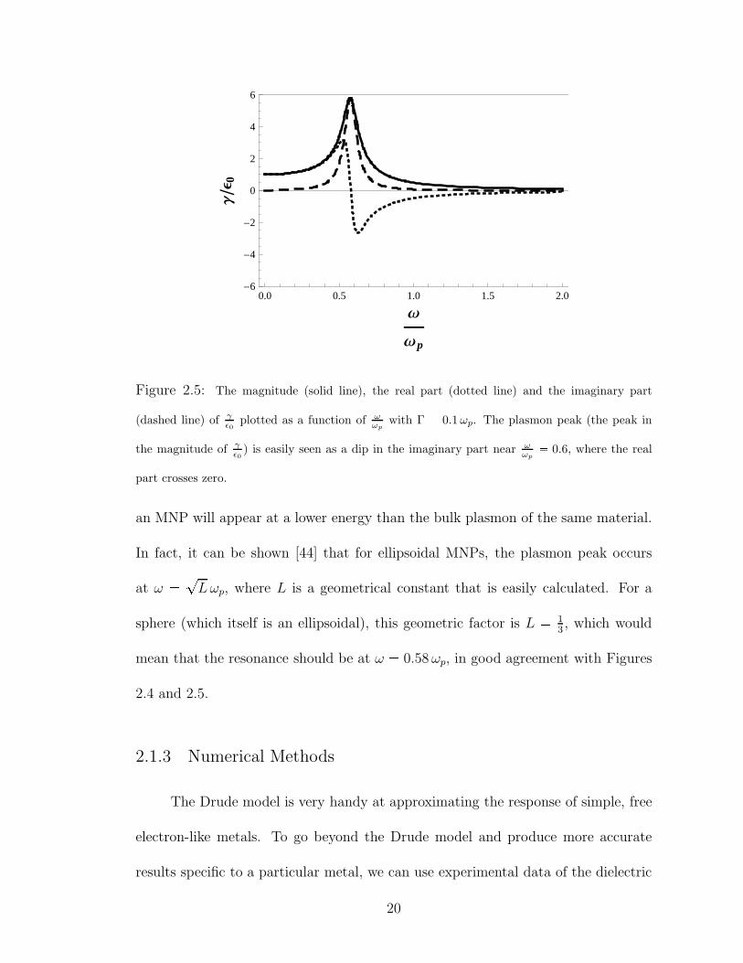
0.6, where the real part crosses zero. . . . . . . . . . . . . . . 192.5 The magnitude (solid line), the real part (dotted line) and the imaginary part
(dashed line) of γǫ0
plotted as a function of ωωp
with Γ 0.1ωp. The plasmon
peak (the peak in the magnitude of γǫ0) is easily seen as a dip in the imaginary
part near ωωp
0.6, where the real part crosses zero. . . . . . . . . . . . . . . 20
3.1 An applied field polarizes both the MNP and SQD which in turn allows for a
dipole-dipole coupling. . . . . . . . . . . . . . . . . . . . . . . . . . . . . 573.2 µ vs. a phase diagram for R 13 nm in the strong field limit. Outlined are
the four distinct regions of system response, namely Fano, EXIT, Suppression
and Bistability. Points denote parameter values for which the system response is
plotted in Figures 3.3, 3.4, 3.6, 3.8, and 3.9. . . . . . . . . . . . . . . . . . . 693.3 Region I. Absorption rate of the MNP, QMNP , shows a Fano shape in the response
due to the phase change in dipole moment of the SQD. This phase change is shown
in the real part of the SQD dipole moment in the right inset. Left inset shows
the sharp dip in the population difference at resonance. Parameter values used
in the calculation were R 13 nm, a 3 nm, and µ 0.25 enm. . . . . . . . . 703.4 Region II. Absorption rate of the MNP, QMNP , shows an exciton induced trans-
parency due to the phase change in the dipole moment of the SQD when the
local field incident on the MNP from the SQD is larger than the applied field.
Right inset shows the real part of the SQD dipole moment which undergoes a
phase change at resonance. Left inset shows the dip in the population difference
at resonance. All three plots show a general broadening relative to region I. The
arrow indicates the second dip in QMNP which is cannot be discerned on this
scale. R 13 nm, a 3 nm, µ 2 enm. . . . . . . . . . . . . . . . . . . . 723.5 The emergence of the modified Fano shape is due to EC crossing zero. This
occurs when the internal field can be larger than the external field. When this
field is then squared to find the absorption, the location where EC crosses zero
can produce a transparency. . . . . . . . . . . . . . . . . . . . . . . . . . 74
v
3.6 Transition region: weak suppression. Here we see the beginning of the suppression
in the response of the SQD, apparent in a slight asymmetry in ∆. Γb 98 µeV,
Γa 37 µeV, with suppression factor S 2.65. The double peaked EXIT
structure is still visible, but the second peak is much smaller relative to the main
peak. The system response is also much broader than in region I or II. Parameter
values R 13 nm, a 7 nm, and µ 1 enm. . . . . . . . . . . . . . . . . . 753.7 The relative strengths of the two main interactions that drive the SQD. ρ12G, the
self interaction, and Ω, the applied field and the MNP response to the applied
field, vs µ for fixed MNP radius (a 7 nm) and frequency (ω 2.5 eV). Note: G
and Ω are nearly constant over the range of frequencies that we are interested in
due to the broad plasmon peak. . . . . . . . . . . . . . . . . . . . . . . . . 773.8 Transition region: Strong suppression. Here the suppression has grown large
enough that a discontinuity has developed in the diagonal and off-diagonal den-
sity matrix elements as well as the energy absorption of the MNP. Also, the trans-
parency in the response due to EXIT no longer approaches zero due to extreme
broadening of the response. Γb 217 µeV, Γa 3 µeV, S 72.3. Parameters:
R 13 nm, a 7 nm, µ 2 enm. . . . . . . . . . . . . . . . . . . . . . . 783.9 Region III. Power absorption density of the MNP with R 13 nm, a 7 nm,
µ 3 e nm and the initial conditions Ap0q 0, Bp0q 0, ∆p0q 1. Left inset
shows a population difference of about 0.8 at resonance and a very broad and
suppressed response in the SQD that is shifted 0.5meV from the bare resonance
of the SQD. Right inset shows that the dipole moment of the SQD slowly changes
sign at this shifted resonance. . . . . . . . . . . . . . . . . . . . . . . . . . 803.10 Region III. Power absorption density of the MNP with R 13 nm, a 7 nm,
µ 3 e nm and the initial conditions Ap0q 0, Bp0q 0, ∆p0q 0. The
bistability causes discontinuities in the responses of the MNP, the SQD and the
population difference. . . . . . . . . . . . . . . . . . . . . . . . . . . . . 813.11 Schematic representation of initial conditions vs. frequency. γ1 represents the
continuous steady state, γ2 represents the discontinuous steady state and γ3 rep-
resents unstable steady state. Note that γ2 and γ3 only exist inside the frequency
interval pω0 δ, ω0 δq. Arrows show how particular initial conditions evolve to
one of the three solutions. Inset show a cross section in ω-space. Points arbitrarily
close to γ3 evolve to γ2. . . . . . . . . . . . . . . . . . . . . . . . . . . . 833.12 Depiction of phasors in the complex plane for a 7 nm. (a. and b.) µ 2 enm.
Suppression region. (a) below resonance (ω 2.4999 eV) and (b) above resonance
(ω 2.5001eV). (c. and d.) µ 3 enm. Region III. (c) below resonance
(ω 2.4996 eV) and (d) above resonance (ω 2.4999 eV) (note: resonance has
shifted to 2.49975eV at this point). The phase of G and Ω are nearly constant.
Moving left to right (i.e. below to above resonance), we see the real part of ρ12
changes sign. This is the phase shift associated with a damped, driven harmonic
oscillator. . . . . . . . . . . . . . . . . . . . . . . . . . . . . . . . . . . 88
vi
3.13 A, the real part of the SQD dipole moment for µ 4 enm, a 5.8 nm at
t 10 ns. Left insert: The system starts in the ground state. Right insert:
The system starts in a mixed state, ∆ 0. Center: an overlay of the two. The
location of the phase crossing for the SQD dipole moment is dependent on the
initial conditions. . . . . . . . . . . . . . . . . . . . . . . . . . . . . . . 903.14 (Top) The real and imaginary parts respectively of solution to the cubic equation
that determines the frequency at which A changes sign (plotted for µ 4 enm).
Up to a 6.3 nm, there is one real solution and two complex solutions (which
are conjugates of each other). In this region, the only real solution is ωω0 0.
For a ¡ 6.3 nm, three real solutions exist. (Bottom) The real part of SQD dipole
moment for µ 4 enm, a 5.8 nm, plotted for 10 ns, 20 ns and 40 ns evolutions
respectively. We see that although for finite time, A has a continuous crossing
through zero, as the system evolves to the steady state, the crossing becomes
discontinuous. . . . . . . . . . . . . . . . . . . . . . . . . . . . . . . . . 923.15 The effect of polarization on the response of the MNP in region II (R 13 nm,
a 3 nm and µ 3 e nm). Curve labeled sα 2 is for the applied field parallel
to the main axis of the molecule, sα 1 for perpendicular polarization. Both
show an EXIT structure. . . . . . . . . . . . . . . . . . . . . . . . . . . . 93
4.1 An applied field polarizes both the MNP and SQD which in turn allows them to
couple. . . . . . . . . . . . . . . . . . . . . . . . . . . . . . . . . . . . 984.2 The real and imaginary parts of G with R 60 nm and a 40 nm, shown for both
a full electrodynamical calculation using the boundary element method (labeled
as BEM) and a non-retarded multipole expansion (labeled Multipole). In this case
we see an enhancement in the imaginary part of G, and a slight enhancement and
red shift of the peak in the real part of G. . . . . . . . . . . . . . . . . . . . 1084.3 Ratio of the magnitude of G as calculated with a full electrodynamical calculation
using the BEM to that of the multipole expansion at a frequency of 2.5 eV which
is near the plasmon resonance for an Au sphere. The value given by the BEM
increases in relation to that of the multipole as the MNP radius is increased for
fixed separation up to a MNP radius of approximately 50nm (except in the most
extreme cases of very small separation) or if the separation is increased for fixed
MNP radius. . . . . . . . . . . . . . . . . . . . . . . . . . . . . . . . . . 1094.4 The real and imaginary components of G and Ω for various values of the wire
length. The width of the wire was fixed at 14 nm, thus the L 14 nm setup is
that of a 7 nm radius sphere. Ω shows a redshift as well as an enhancement in the
response as the length is increased. G shows a redshift as well as the appearance
of higher order modes. For L 150 nm, Ω has 2 peaks, one at 1.1 eV and one
close to 2.1 eV. However, in addition to those 2 peaks, G shows an additional
peak around 1.7 eV for L 150nm. . . . . . . . . . . . . . . . . . . . . . . 1114.5 Response of a 70 nm wire. Both G and Ω are peaked near 1.6 eV. However, we
also see a strong response in G between 22.5 eV, whereas there is no appreciable
response in Ω over that range of frequencies. The peak near 2.2 eV in the real
part of G is evidently a “dark” mode. . . . . . . . . . . . . . . . . . . . . . 112
vii
4.6 Magnitude of time average of electric field squared of 70 nm nanorod excited by
a planewave and dipole source. The dipole source was placed 5 nm above the tip
of the wire with a dipole moment of 1 e nm. (top) For the bright mode at 1.6 eV,
there are hot spots in excess of 20 times the applied electric field for both the
dipole and planewave. (bottom) The dark mode at 2.2 eV responds to the dipole
source, but shows nearly no response to the planewave. . . . . . . . . . . . . . 1144.7 The ratios of GΩ and GIΩ shown for a 70nm length, 14 nm width nanorod
(solid line) and a 7 nm radius spherical MNP (dashed line), with µ 1.0 enm.
These two ratios play a large role in determining the system behavior. . . . . . 1154.8 Bright state, with an exciton energy level at 1.6 eV, L 70 nm, w 14 nm,
µ 0.5 enm. Absorption rate of the MNP, QMNP , population difference, ∆,
and the real part of the SQD dipole moment, A, all show a very strong and broad
response of the system. . . . . . . . . . . . . . . . . . . . . . . . . . . . . 1174.9 Dark state, with an exciton energy level at 2.2 eV, L 70nm, w 14 nm,
µ 0.5 enm. Absorption rate of the MNP, QMNP , and the real part of the
SQD dipole moment, A, both show a bistability in the system. The population
difference, ∆, shows a discontinuity and strong suppression in the excitation of
the SQD. . . . . . . . . . . . . . . . . . . . . . . . . . . . . . . . . . . 1184.10 Near field of a 5 nm radius spherical MNP interacting with a SQD located 10
nm away from center for 3 values of applied frequency. Shown in color is the z
component of the electric field. The first plot shows a strong dipole field from
the SQD, in-phase with the applied field that penetrates the MNP to a depth
of 2 nm. The middle plot show the system at resonance and the appearance
of the exciton induced transparency in the MNP. The third plot shows a strong
dipole field from the SQD, now out-of-phase with the applied field, that again
penetrates the MNP to a depth of 1 nm. . . . . . . . . . . . . . . . . . . . 121
5.1 An applied field induces a polarization in the MNP and both SQDs, which in
turn allows for a dipole-dipole coupling between the three particles. . . . . . . . 1275.2 Energy absorption due to the MNP, energy absorption due to the SQD, and the
total energy absorption, respectively, as a function of detuning, for two SQDs
coupled to a spherical MNP (top), and for a single SQD coupled to a spherical
MNP (bottom). All calculations were in the weak field limit and particle sepa-
ration was varied (the two SQD case was treated symmetrically, R R1 R2,
µ µ1 µ2 and ω0 ω1 ω2). In both sets of plots we take a 7.5 nm and
µ 0.5 enm. . . . . . . . . . . . . . . . . . . . . . . . . . . . . . . . . 1345.3 µ vs. a phase diagrams in the strong field limit for an SQD-MNP system (bottom)
and an SQD-MNP-SQD system (top). Single SQD system shows 4 regimes of
behavior and SQD-MNP-SQD system shows 5 regimes of hybrid behavior. In
both plots, the SQD-MNP separation was 13 nm. . . . . . . . . . . . . . . . 1365.4 Density matrix elements plotted as a function of detuning for two interacting,
strongly coupled SQDs (a 0 nm, µ1 µ2 3.0 enm and R1 R2 13 nm).
The response of the system shows discontinuity for detunings near 0.05meV. For
these frequencies, the system no longer reaches a steady state. . . . . . . . . . 138
viii
5.5 ρ11 plotted as a function of the detuning between the driving field and SQD1 for
four cases of explicit symmetry breaking. In all cases a 0 nm, µ1 3.0 enmand R1 R2 13 nm were held fixed. The top two plots show µ2 Ñ µ1 δ
symmetry breaking with ω1 ω2. The bottom two plots show ω2 Ñ ω1 δ
symmetry breaking with µ1 µ2. . . . . . . . . . . . . . . . . . . . . . . . 1415.6 Evolution of ρ11 as a function of time, for a 0 nm, µ1 µ2 3.0 enm, R1
R2 13 nm, and ω1 2.5 eV, for a driving frequency in the chaotic regime
(ωω1 0.75meV). Shown are the oscillations for an explicit symmetry breaking
of ω2 ω1p1 106q (top) and ω2 ω1p1 108q (bottom). Insets shows that
the frequency of oscillation does not appear to depend on the amount of the
symmetry breaking. . . . . . . . . . . . . . . . . . . . . . . . . . . . . . 142
5.7 Time evolution of ρ22, ρ33, ρSS and ρAA, for a 0 nm, µ1 µ2 3.0 enm,
R1 R2 13 nm, ω1 2.5 eV and ω2 ω1p1 106q, for a driving frequency
in the chaotic regime (ω ω1 0.75meV). ρ22, ρ33, and ρSS are initially driven
and quickly oscillate, while ρAA slowly fills due to relaxation. . . . . . . . . . . 1435.8 The secondary oscillations occur over a range of the applied frequencies (ω
ω0 0µeV to 200µeV, ω0 ω1 ω2). The onset of the oscillations occurs
sooner for frequencies near the end points of this window, reaching a maximum
onset delay at approximately ω ω0 80µeV. In all cases the other system
parameters and initial conditions are held fixed (µ1 3.25 enm, µ2 3.27 enm,
R1 R2 13nm, ω0 ω1 ω2 2.5 eV) . . . . . . . . . . . . . . . . . . . 1455.9 The onset of chaotic behavior as a function of detuning for three regimes of
symmetry breaking, µ2 µ1 p1 10nq with n t2, 6, 10u, plotted for each of
µ1 3.0 enm (bottom), µ1 3.1 enm (middle) and µ1 3.3 enm (top). For
each of the three plots, we see that the delay in the onset increases as the mag-
nitude of the symmetry breaking decreases. When the three plots are compared,
the peak in the onset appears to shift to a larger detuning (from ωω0 90µeV
to ωω0 100µeV) as the magnitude of µ1 (and thus µ2) increases from 3.0 enmto 3.3 enm. . . . . . . . . . . . . . . . . . . . . . . . . . . . . . . . . . 147
5.10 Density matrix for a quantum mechanical coupling between the dots. In this
model, the chaotic regime disappears. µ1 3.0 enm, µ2 µ1p1 103q, R1 R2 13 nm, ω0 ω1 ω2 and a=0. Compare to the plot in the upper left-hand
side of Figure 5.5. . . . . . . . . . . . . . . . . . . . . . . . . . . . . . . 1525.11 Dipole blockade measure, β, as a function of the detuning for various values of
system parameters. Blockade increases with decrease in dot-to-dot separation
(increased coupling) and decreases with response broadening (increased couping
to the driving field or MNP). (ω0 ω1 ω2) . . . . . . . . . . . . . . . . . 1545.12 Comparison of semiclassical model (top 6 plots) and quantum model (bottom
6 plots) in the regime with weak SQD-SQD coupling (µ1 µ2 0.5 enm),
and strong SQD-MNP coupling (a 7 nm, R1 R2 13 nm). Shown are the
diagonal density matrix elements (ρ11, ρSS, ρAA, ρ44) and the blockade measure,
β. Also shown are the real (solid line) and imaginary (dotted line) parts of the
transition dipole moment of the symmetric state, µSS ρ1S ρS1 ρS4 ρ4S. . . 158
ix
Chapter 1
Background and Motivation
1.1 Introduction
On December 29, 1959, Richard Feynman gave his now famous talk “There’s
Plenty of Room at the Bottom” at the APS annual meeting at the California In-
stitute of Technology [1]. He spoke of the possibilities that miniaturization could
bring to data storage, atomic and molecular manipulation and synthesis, and even
nanomachines and nanorobotics. He challenged scientists of the day to improve
upon the 1 nm resolution size of the scanning electron microscope (SEM). He also
made the prediction that a single bit of information could someday be stored with
the use of only 100 atoms, meaning that less than 1000 atoms would be needed to
store a single alphanumeric character in 8-bit binary.
The scanning tunneling microscope (STM) was developed by Binnig and Rohrer
in 1981 [2] with a resolution size approximately ten times smaller than that of an
SEM. By the end of the decade, Eigler and Schweizer [3] used an STM to demon-
strate a single atom manipulation technique that allowed them to write out “IBM”
using letters that were approximating 5 nm in height, and all three letters consisted
of only 35 atoms, surpassing even Feynman’s bold prediction. With this not so
humble beginning, the advent of nanotechnology truly began.
Nanotechnology is more than just the imaging and manipulation of objects on a
1
Figure 1.1: An artist’s rendition of a C60 buckminsterfullerene. Each of the black dots represents
a single carbon atom. Graphic generated using Mathematica software.
nanometer scale. Also included under this broad heading is the development of new,
novel, nanoscale structures and materials, which due to their size and composition
can possess unique properties. In 1985, Kroto, et. al. discovered C60 buckminster-
fullerene, a molecule consisting solely of 60 carbon atoms with each atom bound
to three others and forming a spherical shell [4] (see Figure 1.1). This pattern of
bonding forms a structure of pentagons and hexagons that alternate throughout the
object in a familiar soccer ball pattern. This molecule turned out to be just one
member in a larger family of molecules which are now known as fullerenes. The
most common of the fullerenes are the buckyballs (which includes the aforemen-
tioned C60, as well as the similar structures C24, C28, C32, C36, C50, C70, etc
[5]).
Another type of fullerene is the carbon nanotube [6]. These objects are the
two-dimensional analog of buckyballs. A carbon nanotube has the same pattern
2
of carbon binding as the buckyballs, however, instead of having a spherical shape,
they are rolled up in a cylinder- like a cigar. These nanotubes often have a diameter
around 1 nm with a length that can reach a million times that, and contain millions
of carbon atoms.
One thing that makes carbon nanotubes particularly interesting is that one
dimension (the circumference of the cylinder) is very small and very quantum me-
chanical, and the other dimension (its length) is very large, reaching millimeter
scales, i.e. the macroscopic world. So from the scale of a few atoms to that of a
30 cm long carbon nanotube, we can say that the study of nanoscale physics is the
study of the boundary between classical and quantum mechanics.
1.2 Nanoparticles
The focus of this thesis will be hybrid systems made from semiconducting
nanoparticles [7, 8] and metal nanoparticles [9, 10]. These systems can often ex-
hibit characteristics of both the quantum and classical regimes. Furthermore, the
boundary between classical and quantum can be defined by the particles, i.e. the
semiconducting nanoparticles can behave more quantum mechanically and the metal
nanoparticles can behave more classically. Such nanoparticles are objects typically
1100 nm in size, often approximately spherical in shape, and composed of atoms in
the bulk form for the material rather than the highly ordered and hollow structure
of the fullerenes. Nanoparticles can have novel properties due to their extremely
small size. First, there can be confinement effects once the size of the nanoparticle
3
is on the order of the wavelength of its excitation energy. Second, as a particle is
made increasingly small, the ratio of the number of surface atoms of the particle
to those that make up the bulk grows larger. As such, surface effects can come to
dominate the physics of a nanoparticle, whereas they might be ignored in a larger
object of the same composition.
Metal nanoparticles (MNPs) are typically made of a single metal such as gold,
silver or platinum. If an MNP has an oblong shape, like a rod or cylinder, with
a length on the order of 10 1000 nm then it is commonly known as a nanorod.
If a nanorod has a nearly infinite length (on the order of 1µm), it could then be
considered as a nanowire.
A nanoparticle made out of a semiconductor material (most typically InAs,
GaAs, ZnS, ZnSe, CdS, CdSe, CdTe, or HgS) is referred to as a semiconductor
nanoparticle. If the size of a semiconductor nanoparticle is small enough to confine
an electron in the conduction band and also a hole in the valence band, in all
three spatial directions, it is known as a semiconducting quantum dot (SQD). If the
nanorod or nanowire is made from a semiconducting material, then it would be a
quantum wire and would have excitations that were confined in two of the three
directions, while the excitations would be free to propagate in the third.
In this thesis, the metallic nanoparticles that we will consider will range in
size from just a few nanometers to 100 nm or more. Metals of this size consist of
very many electrons. Due to this, it will be valid to treat the MNPs we consider
to be classical in nature. The SQDs that we will consider will be slightly smaller
in size than the MNPs. However, the size of the SQD has little effect on how it is
4
modeled. Most important is the confinement of the electron inside the SQD, which
requires the SQD to be modeled quantum mechanically.
1.3 Nanosuperstructures
A structure made from a few or many nanoscale objects is often called a
nanosuperstructure [11, 12, 13]. Such a physical system could have unique prop-
erties, and they could be engineered to suit a particular task. Recent advances in
nanoscience have already allowed for the construction and study of such nanosuper-
structures. By using various combinations of the available building blocks (nanowires,
semiconductor quantum dots, metal nanoparticles, biolinkers, etc.) to create hybrid
molecules, novel physical phenomena may be explored. Such structures will allow
the study of physics at the interface of classical and quantum mechanics and could
provide the technology for a number of devices in the field of quantum information.
These structures should allow for the physical transportation of excitations as well
as the transportation of coherent states.
Experiments have already demonstrated the plausibility of creating and study-
ing such superstructures. Recently, researchers have shown that using a lithographic
process, it is possible to control the deposition of quantum dots near nanowires [14].
This two step process, one of which results in a polymer template, should make
more complicated structures accessible in the near future.
Recently, hybrid structures consisting of a quantum dot and a metal nanopar-
ticle joined by a biolinker have been assembled and studied [15]. Experimental
5

investigations have shown efficient exciton-plasmon-photon conversion and an en-
hanced emission rate with the coupling of a CdSe quantum dot to a silver nanowire
[16, 17]. Furthermore, when coupled to elongated MNPs, the photoluminescence in-
tensity of SQDs is enhanced in a polarization-selective way [18], and when coupled
with a nano-optical Yagi Uda antenna the SQD emission can be made unidirectional
[19].
Hybrid structures consisting of an SQD and an MNP are a very active area
of research in theoretical physics [15, 20, 21, 22, 23, 24, 25, 26, 27, 28, 29, 30].
By coupling the broad continuous plasmonic response of the MNP to the discrete
excitons of the SQD, these structures allow the study of systems at the interface
between classical and quantum physics. Furthermore, such structures could allow
for the directed nanoscale transmission of information and excitations.
In this thesis, we will examine the physics of nanohybrid molecules, in particu-
lar those formed with metallic nanoparticles and semiconductor quantum dots. We
hope to learn how the presence of a nearby SQD affects the response of an MNP.
The MNP, with its ability to enhance local fields, will certainly have a large effect
on a nearby quantum dot. We will study how the behavior of these nanoparticles
changes when they are combined in hybrid structures in Chapters 3 and 4 of this
thesis.
6
1.4 Transmission of Quantum Information
Once we allow for systems consisting of more than one nanoparticle, we must
then consider how excitations are transferred between nanoparticles. The nanoscale
transmission of quantum information and excitations between qubits for quantum
communication, quantum computing and quantum measurement will require trans-
fer where the quantum character of the information can be maintained.
At submicrometer distances, this means directed transmission must be carried
out with better than wavelength scale resolution. One possible solution to this lim-
itation is coupling qubits, for example in quantum dots, to plasmonic structures. It
has been predicted that below the diffraction limit, highly efficient directed energy
transfer over plasmonic wires consisting of chains of closely spaced metal nanopar-
ticles could be achieved [31]. And at larger distances, strong, coherent coupling
between emitters should be possible by means of guided plasmons that are evanes-
cently coupled with a nearby dielectric waveguide[32]. Furthermore, it has been
predicted that large entanglement, either spontaneously formed or in a continu-
ously driven steady state, would be possible between qubits coupled to a plasmonic
waveguide over distances exceeding a wavelength [33].
Several recent experiments have already shown very promising results in these
structures. It has been shown that quantum coherence can survive in plasmonic
structures, such as the transportation of entangled photons by surface plasmons [34]
and the energy-time entanglement of a pair of photons following a photon-plasmon-
photon conversion [35]. Furthermore, it has been demonstrated that during plasmon
7
propagation in metallic waveguides, losses appear to follow a linear, uncorrelated
Markovian model of damping at the single quanta level, showing the quantum regime
of plasmonics is realistic [36]. In related work, the quantum statistics of the light
from a quantum emitter (in this case the color center of a nanodiamond) was shown
to be preserved after conversion to plasmons and propagation in a polycrystalline
gold film [37].
To exploit this paradigm for quantum, nanoscale communication, one must
understand how metallic nanoparticles act as nanoantennas and nanoguides. One
must understand the coupling between dots and plasmons in metallic nanoparticles.
One must also understand how dot-to-dot quantum communication is modified by
transfer via plasmons. Finally, one must understand how transfer is further modified
if the metal nanoparticles are small and quantum effects can influence their response.
To this end, we will consider systems in which the interaction between two spatially
separated quantum dots is mediated by plasmons. This is the subject of Chapter 5.
The layout of the thesis is as follows. In Chapter 2, we discuss how we will be
modeling the MNP and SQD as physical objects, and then we review the necessary
physics and math that we will need to model the interacting system. We then
examine some toy models to highlight some of the technical issues involved in the
study of these systems and to illustrate the manner in which modeling was done for
the work presented in this thesis. In Chapter 3, we model a realistic hybrid system
consisting of an SQD coupled to a nearly spherical MNP. The two particles are
driven by an oscillating electric field which in turn causes a dipole-dipole coupling.
We will examine the optical response of the system in both the weak field regime
8

and in the strong field regime. Furthermore, we will discover four distinct regimes of
behavior that depend on the strength of the SQD-MNP coupling, as we first reported
in [21] and expanded upon in [22]. In Chapter 4, we will see how the dependence
of local field enhancement strength on MNP shape could be exploited to engineer
MNP-SQD hybrids that are biased towards a desired type of hybrid response. These
results were first reported by us in [38]. In Chapter 5, we look beyond two particle
MNP-SQD systems and look at the ways in which we can model a more complicated
SQD-MNP-SQD system. Finally, in Chapter 6, I present my conclusions and briefly
discuss the outlook and future work to be done to further our knowledge on these
and similar systems.
9
Chapter 2
Tools and Toys
The system we wish to study consists of an SQD and an MNP separated by
some distance with both particles subject to an applied optical field (as shown in
Figure 2.1). We imagine that both particles have resonances near the energy of
the applied field, and we will then model how the presence of the one effects the
response of the other. To this end, we will describe techniques needed to model
hybrid nanoparticle systems. Although we are focused on systems consisting of
MNPs and SQDs, much of what will be discussed here is applicable to a much
broader group of systems, especially those that operate in the visible or near-visible
spectrum and in which losses and decoherence must be accounted for.
Figure 2.1: An MNP and an SQD subject to an applied optical field.
We begin this chapter with brief descriptions of MNPs. We then proceed to
10
model their plasmonic resonances using a Drude model, and we then show how to
use experimental data to build a response function. We then discuss SQDs and
confinement effects, and show how SQDs can be treated like atoms. In the next
section, we look at open quantum systems. In order to study our MNP-SQD system,
we will need to account for the interaction of our system with its environment.
With this as motivation we introduce the density matrix formalism of quantum
mechanics. We next concern ourselves with the interaction of light and matter in
order to better understand the interaction of the SQD with the field. We develop
the dynamical equations that govern the time evolution of the system. After a first
attempt to model the interaction, we see that allowing for spontaneous emission is
necessary for the interaction. We then build a quantum theory of open systems in
the Lindblad formalism. The use of the theory is illustrated with a simple system
prior to it being generalized for the quantum optics regime. We then use the tools
we have just developed to model a system consisting of an atom in an oscillating
electromagnetic field. Finally, the chapter is concluded with a discussion on how
numerical calculations were performed to evaluate the set of dynamical equations
we study.
2.1 Metallic Nanoparticles
Although metallic nanoparticles have been used since ancient times to color
glazed pottery and stained glass, it wasn’t until Faraday’s work with gold particles in
an aqueous solution in the 1850s [39] that this effect was attributed to the particles’
11

small size. Although Farady was the first to show that these small particles of
gold could have very different optical properties than those of bulk gold, a full
understanding of the process was not presented until 1908 when Mie published his
seminal paper on the scattering of such small objects [40]. This scattering process
later became known as Mie scattering. By considering the scattering of an incident
planewave of light off of a sphere, Mie was able find a series solution to Maxwell’s
equations in the regime where the particle’s size is on the same order as in the
incident light. This is in contrast to Rayleigh scattering which assumes the particle
to be much smaller than the wavelength of incident light [41].
A key feature of MNPs is that they can support surface plasmons. Surface
plasmons are the quasi-particle of coherent oscillations of electron density on the
surface of a metal and were originally studied by Ritchie on the surface of thin
films [42]. On a film or other bulk material, the plasmons propagate along the
surface when excited by incident radiation via a coupler, e.g. a grating. In an
MNP however, because the size of the metal is smaller than the wavelength of the
incident light (often by an order of magnitude or more), the plasmons are unable
to propagate and are thus confined. Because of this confinement, the response of
a MNP is highly dependent on the wavelength of incident light. For a spherical
gold MNP, the response has a maximal peak in the vicinity of 2.3 2.5 eV. This
resonance is the dipolar plasmon peak. This resonance causes a build up of charge
on the surface of the particle, enhancing not only the scattering and absorption of
the incident light, but also producing a dipolar response field (in the small particle
limit, in general higher orders of the multipolar expansion are also present). This
12
dipole field can display very large enhancement of the incident field near the surface
of the MNP.
2.1.1 Modeling the MNP response to a planewave
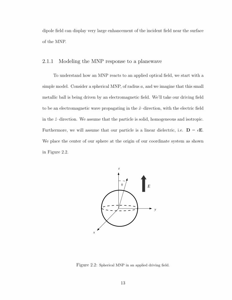
To understand how an MNP reacts to an applied optical field, we start with a
simple model. Consider a spherical MNP, of radius a, and we imagine that this small
metallic ball is being driven by an electromagnetic field. We’ll take our driving field
to be an electromagnetic wave propagating in the x–direction, with the electric field
in the z–direction. We assume that the particle is solid, homogeneous and isotropic.
Furthermore, we will assume that our particle is a linear dielectric, i.e. D ǫE.
We place the center of our sphere at the origin of our coordinate system as shown
in Figure 2.2.
Figure 2.2: Spherical MNP in an applied driving field.
13
Since our particle is very small, on the order of 10 nm or so, much smaller than
the wavelength of visible light (390–750 nm), we assume that the field, at any partic-
ular moment in time, is approximately constant throughout the MNP. This ‘quasi-
static’ approximation allows us to ignore retardation effects. Thus, we must calculate
the electric field produced by a spherical dielectric particle, Eresponsepx, y, zq, by a
constant applied electric field, Eappliedpx, y, zq E0z.
Now, if our particle is not a magnetic material, and we are using the quasi-
static approximation, we solve Gauss’ law in the absence of charges, ∇ ǫE 0.
To do so, we first define the scalar potential, V, such that E ∇V. In terms of
V then, we have ∇2V 0, which is simply Laplace’s equation. Solving Laplace’s
equation in this case is best done in spherical coordinates. The solution to Laplace’s
equations with azimuthal symmetry is a sum of Legendre polynomials [43],
Vpr, θq 8n0
Anr
n Bn
1
r
n1Pnpcos θq (2.1)
where the coefficients An and Bn are determined by the boundary conditions. There-
fore, we can write our solution like this:
V $'''&'''%°8n0
An
ra
n Bn
ar
n1Pnpcos θq for r a ,°8
n0
A1
n
ra
n B1n
ar
n1Pnpcos θq for r ¥ a.
(2.2)
Inside the MNP, nonzero values for the Bn would lead to an unphysical infinite
potential at r 0, so we can take Bn 0 for all n. We also require that far from the
MNP, the potential approaches that of the applied field, Eapplied, so V Ñ E0r cos θ
for r ¡¡ a. Therefore, for r ¥ a we must have A11 aE0 and, A1
n 0 for n 1.
14
Our potential is now
V $'''&'''%°8n0An
ra
nPnpcos θq for r a ,°8
n0B1n
ar
n1Pnpcos θq E0r cos θ for r ¥ a.
(2.3)
Further boundary conditions that must be met are the continuity of V and the
normal component of D at the dielectric interface. From the first we have8n0
AnPnpcos θq 8n0
B1nPnpcos θq E0a cos θ. (2.4)
In regards to the latter, the normal component of D at the MNP surface is pro-
portional to BVBr . So, we must have BVBr outside ǫǫ0
BVBr inside, where ǫ is the dielectric
constant of the material the MNP is composed of, and ǫ0 is the vacuum dielectric
constant. From this we can write
ǫ
ǫ0
8n1
nAn
1
aPnpcos θq 8
n1
pn 1qB1n
1
aPnpcos θq E0 cos θ. (2.5)
Using the orthogonality of the Legendre polynomials, our boundary conditions
term by term become
A0 B10
A1 B11 E0a
An B1n , n ¡ 1
and
ǫ
ǫ0A1 2B1
1 E0a
nǫ
ǫ0An pn 1qB1
n , n ¡ 1
15
Since A0 is just the value of the potential at the center of the MNP, we can arbitrarily
set this to zero. Therefore, we can finally write
A0 B10 0
A1 3ǫ02ǫ0 ǫ
E0a
B11 ǫ ǫ0
2ǫ0 ǫE0a
n 1
nAn ǫ
ǫ0An , n ¡ 1
If we assume that ǫ is complex, then the relation n1n
ǫǫ0
does not hold for any
n. Therefore, we must have An 0 for n ¡ 1. Thus our solution is
V $'''&'''% 1ǫeff
E0r cos θ for r a ,
γa3E01r2cos θ E0r cos θ for r ¥ a,
(2.6)
where we have defined ǫeff 2ǫ0ǫ3ǫ0
and γ ǫǫ02ǫ0ǫ
.
We now calculate the total electric field, E Eapplied Eresponse,
E $'''&'''% 1ǫeff
E0
cos θ r sin θ θ
for r a ,
1 2γa3
r3
E0 cos θ r γa3
r3 1
E0 sin θ θ for r ¥ a.
(2.7)
which can be rewritten
E $'''&'''% 1ǫeff
E0z for r a ,
2γa3
r3E0 cos θ r γa3
r3E0 sin θ θ E0z for r ¥ a.
(2.8)
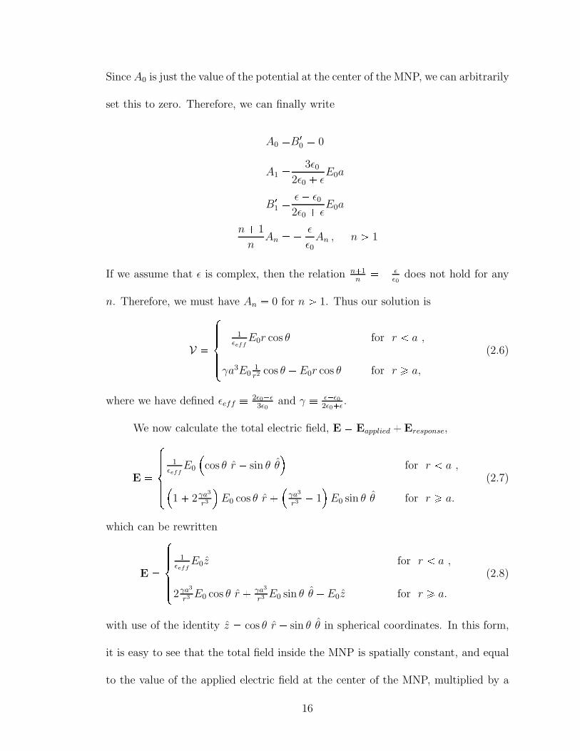
with use of the identity z cos θ r sin θ θ in spherical coordinates. In this form,
it is easy to see that the total field inside the MNP is spatially constant, and equal
to the value of the applied electric field at the center of the MNP, multiplied by a
16
‘screening’ factor, 1ǫeff
. Outside the MNP, the total electric field easily splits into
Eresponse Eapplied, and we see that Eresponse in this region is
Eresponsepr ¥ aq 2γa3
r3E0 cos θ r γa3
r3E0 sin θ θ. (2.9)
We can rewrite this as
Eresponsepr ¥ aq γa3r3E0
2 cos θ r sin θ θ
γa3r3E0
2 cos θ r sin θ θ cos θ r cos θ r
γa3r3E0 p3 cos θ r zq 1
r3p3pµMNP rq µMNPq (2.10)
where we have defined µMNP γa3Eapplied. The astute reader will recognize that
equation (2.10) is identical to the field produced by a dipole located at the ori-
gin, with dipole moment equal to µMNP. This means the applied field induces a
polarization in the MNP, equal to γa3Eapplied.
Therefore, we have shown that in this limit, for a particular driving field, the
field inside the MNP is determined by the screening factor 1ǫeff
. Outside of the MNP,
for a particular driving field and particle radius, the response is determined by γ.
Thus when we speak of the response of an MNP, what we really need to know are
these two functions. Because ǫeff determines the field inside the MNP, we can also
say that it determines the absorption of the MNP. Likewise, since γ determines the
field external to the MNP, it determines the scattering of the MNP.
17
0.0 0.5 1.0 1.5 2.0-10
-5
0
5
10
Ω
Ωp
Ε0Ε
Dru
deHΩL
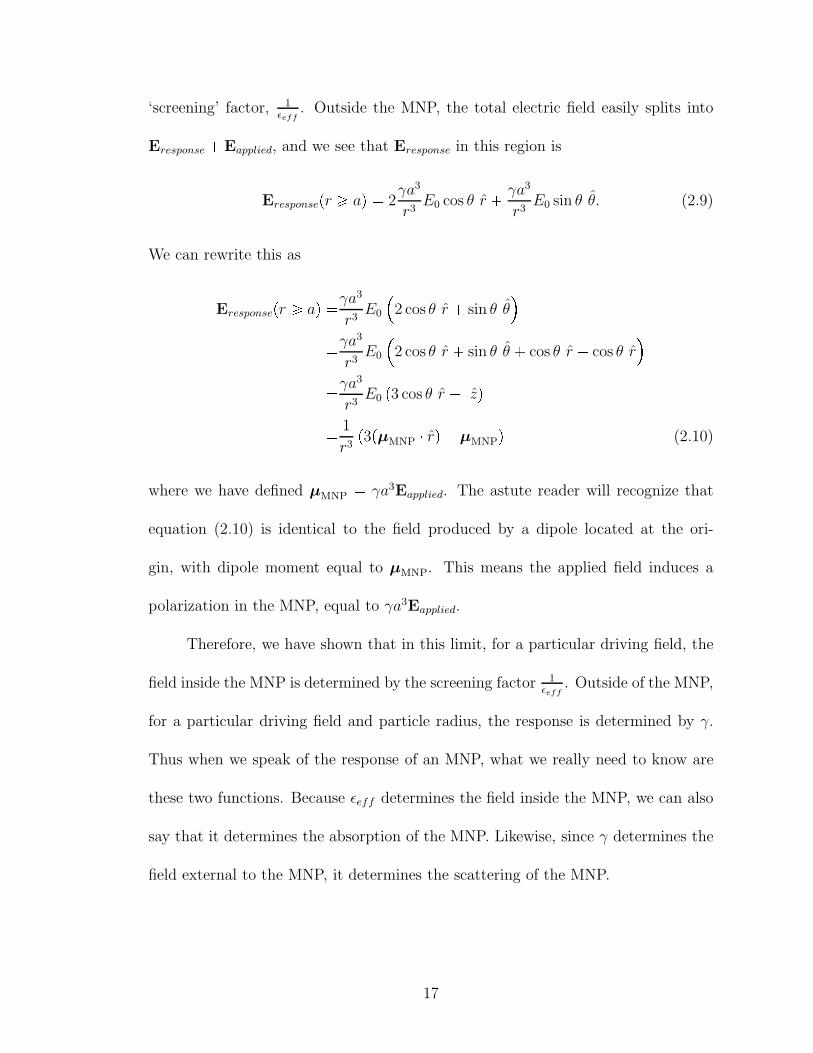
Figure 2.3: The magnitude (solid line), the real part (dotted line) and the imaginary part (dashed
line) of ǫ0ǫDrude
plotted as a function of ωωp
with Γ 0.1ωp. The plasmon peak (the peak in the
magnitude of ǫ0ǫDrude
) appears at a dip in the imaginary part at ωωp
1, where the real part crosses
zero.
2.1.2 The Drude Model
Both γ and ǫeff are determined by the dielectric of the MNP, ǫ. What makes
this particularly interesting is that ǫ is a function of the driving field frequency ω. A
well-known way to model this dependence of ǫpωq is with a Drude model for metal
[44],
ǫDrudepωqǫ0
1 ω2p
ω2 iωΓ1 ω2p
ω2 Γ2 i
Γω2p
ωpω2 Γ2qThe bulk plasmon frequency, ωp, is defined as ωp b
ne2
meǫ0, where e and me are the
electron charge and mass respectively and n is the density of electrons in the metal.
Damping in the model is accounted for by Γ which is related to the mean free path
18
0.0 0.5 1.0 1.5 2.0-6
-4
-2
0
2
4
6
Ω
Ωp
Ε0Ε
eff
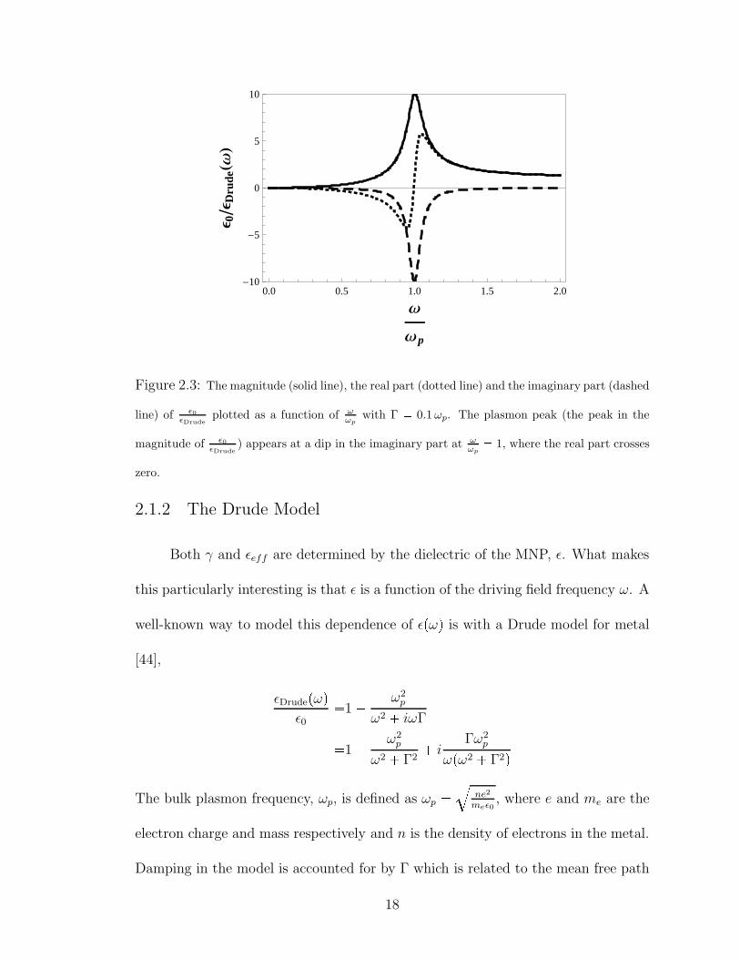
Figure 2.4: The magnitude (solid line), the real part (dotted line) and the imaginary part
(dashed line) of ǫ0ǫeff
plotted as a function of ωωp
with Γ 0.1ωp. The plasmon peak (the peak in
the magnitude of ǫ0ǫeff
) is easily seen as a dip in the imaginary part near ωωp
0.6, where the real
part crosses zero.
of the electrons in the metal and their Fermi velocity.
The Drude model is plotted in Figure 2.3. Shown are the real and imaginary
parts of the dimensionless quantity ǫ0ǫDrude
, plotted as a function of ωωp. We have
chosen the relaxation rate to be an order of magnitude less than the rate of plasmon
oscillations, i.e. Γ 0.1ωp. In the plot, we see that an electric field scaled by a
factor of ǫ0ǫDrude
, would have very large enhancement (about an order of magnitude)
near ω ωp, where the magnitude of this quantity reaches a resonance peak.
We can now use the Drude model for ǫpωq in order to model γ and 1ǫeff
. When
we do, we see that the resonance peak in the response of both (see Figures 2.4
and 2.5) occurs at a lower frequency, near ω 0.6ωp, as opposed to that of 1ǫDrude
which peaks at ω ωp. This is a general feature of MNPs, the plasmon peak of
19
0.0 0.5 1.0 1.5 2.0-6
-4
-2
0
2
4
6
Ω
Ωp
ΓΕ
0
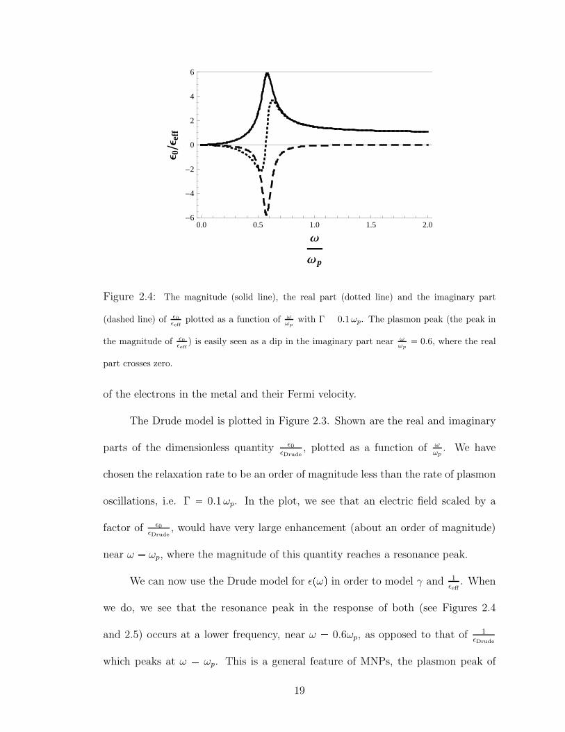
Figure 2.5: The magnitude (solid line), the real part (dotted line) and the imaginary part
(dashed line) of γǫ0
plotted as a function of ωωp
with Γ 0.1ωp. The plasmon peak (the peak in
the magnitude of γǫ0) is easily seen as a dip in the imaginary part near ω
ωp
0.6, where the real
part crosses zero.
an MNP will appear at a lower energy than the bulk plasmon of the same material.
In fact, it can be shown [44] that for ellipsoidal MNPs, the plasmon peak occurs
at ω ?Lωp, where L is a geometrical constant that is easily calculated. For a
sphere (which itself is an ellipsoidal), this geometric factor is L 13, which would
mean that the resonance should be at ω 0.58ωp, in good agreement with Figures
2.4 and 2.5.
2.1.3 Numerical Methods
The Drude model is very handy at approximating the response of simple, free
electron-like metals. To go beyond the Drude model and produce more accurate
results specific to a particular metal, we can use experimental data of the dielectric
20

constant of bulk metals for various values of the driving frequency. Once this data
is obtained for a particular metal, we can interpolate the data to extend the domain
into the regions between data points, to produce a continuous function, ǫpωq. Once
ǫpωq is known, it is a simple matter to calculate γ and ǫeff.
To model structures more complicated than just spheres, solving Maxwell’s
equations in closed form in order to calculate γ and ǫeff is often not possible. To calcu-
late the optical response of such structures, numerical methods of solving Maxwell’s
equations must be employed. Numerical approaches commonly used include the
finite element method (FEM) [45], finite difference time domain method (FDTD)
[46], and boundary element method (BEM) [47], amongst many others.
In this thesis, when modeling the response of nanorods, we will use the BEM,
which has the advantage that it requires less computing resources than volume-
discretization methods such as the FEM or the FDTD. The BEM begins with the
surfaces that form the interface between regions of differing dielectric materials.
Each surface is divided up into small sections by means of a grid. Solutions to
Maxwell’s equations inside each region impose boundary conditions on the interface
surfaces in terms of surface charges and currents. The surface charges and currents
for each element are then matched in a self-consistent way by inverting a very large
matrix. Once the surface charges and currents are known, Green’s functions allow
for the solution to be propagated away from the surface to any point of interest.
Actual numerical calculations performed for the research presented in this
thesis were done using software written by our collaborators at the Donostia Inter-
national Physics Center in San Sebastian, Spain. The software, written in C++,
21
consists of two main programs, the first calculates the response due to a planewave
and the second does the same for a dipole. In both programs, the user specifies
the locations of boundaries between materials of differing dielectric constant. The
location where the resultant field should be calculated is also input. Additionally,
the dipole program requires the location and direction of the test dipole that will
induce the response. Various parameters control the accuracy (and thus run-time)
of the result. Once the BEM software has calculated the response, the fields can
then be used in our models.
2.1.4 Modeling the MNP Response to a Dipole Source
A planewave is not the only type of electromagnetic radiation that our MNP
will be subject to. The field emitted by the SQD will resemble that of a dipole.
To calculate the response of the MNP to a dipole field, we could proceed as before,
by solving Maxwell’s equations in the quasi-static limit. However, the response can
also be quickly approximated using our previous results. If we assume that our
MNP is very small and sufficiently far away from the dipole, then the electric field
has a small variation over the volume of the MNP. If we assume that the field is
approximately constant, then we can approximate the total field inside the MNP
to be Edipoleǫeff, where Edipole is the value of the dipole field at the location of the
center of the MNP. Likewise, the response field outside the MNP will scale with γ.
In making this approximation, we are only allowing the MNP to have a dipole
response to this dipolar field, but higher order modes in the MNP would be excited
22
by the dipole. However, in cases where we need to account for these additional
modes, and go beyond a dipole limit, we can do so by using a multipole expansion
or by the BEM, as we will discuss in Chapter 4.
2.2 Semiconducting Quantum Dots
We begin our examination of the SQD by first looking at semiconductors. A
semiconductor is characterized by the existence of a band gap in its allowed electron
energy levels. Physically, the band gap is the difference in energy between the valence
and conduction electrons. When energy is added to the semiconducting material, for
example when an electric field is applied across it, electrons from the valence band
may move up into the conduction band and can flow through the material, i.e. they
conduct. However, as a semiconductor is made increasingly small, conduction band
electrons increasingly find less room in which to flow. Thus the electrons become
confined.
Since we are imagining that our nanoparticle is very small, we can model
the conduction band as an electron trapped in an infinite square well. Then the
electron’s wavefunction for the state with quantum numbers pnx, ny, nzq isΨpnx, ny, nzq d
8
lx ly lzsin
nxπx
lxsin
nyπy
lysin
nzπz
lz(2.11)
with energy
Epnx, ny, nzq π2~2
2m
nx
lx
2 ny
ly
2 nz
lz
2. (2.12)
Thus we see that as lx , ly , and lz are made ever smaller, the spacing between the
energy levels increases (this holds true regardless of particle shape). This allows
23
for us to create a quantum dot in which only the lowest energy level is effectively
reachable, with all higher energy levels beyond typical electron energies for the
system. For example, if we irradiate a quantum dot with a field that is on resonance
with the energy gap between the valence and first conduction band state, then once
the first electron is knocked into the conduction band, ignoring the degeneracy of
the electron spin, no further electrons will be excited since the energy gap between
the valence band and the second conduction band state will be far detuned from
wavelength of the applied field.
Once we have a single electron in the conduction band, there is a hole that
is left behind in the valence band, which is also quantized, where the electron once
was. Since the electron has negative charge, the hole has a positive charge and
thus they are attracted to one another and can form a bound state. This bound
pair of an electron and its hole is called an exciton. As this is an attractive force,
it contributes a negative energy to the energy of the excited state. Additionally,
there is an effective confinement energy for both the electron and the hole. Thus we
have three sources of energy contributing to the exciton energy, the band gap, the
confinement and the electron-hole coulomb interaction.
To model an SQD, we assume that it possesses some excitonic energy level,
which is determined by its size and the actual material it is composed of. This
energy is typically in the range of 14 eV which makes the quantum dot an excellent
candidate to study in quantum optics. Furthermore, we will assume that any laser
or source of radiation that our SQD is in contact with will be very close in resonance
to this exciton energy. As long as that is the case, we assume that higher energy
24
levels are not excited and we effectively have a two level quantum system, i.e. there
is an exciton, or there is not.
2.3 Quantum Open Systems
In order to study realistic quantum systems, it is often necessary to restrict the
size of the system under study. In our case, we will be modeling the interactions of
the MNP and SQD, as they respond to the applied electric field, and to each other.
However, there are other interactions that would have an effect on our system if such
a system were studied in a lab. Both the MNP and SQD would have phonon modes
that could influence behavior. Most importantly, the exciton has a finite lifetime.
It spontaneously decays. In order to account for these effects, all other physical
interactions and processes that are not included in our system are then given as
properties of a reservoir or a “bath”. We will define an open quantum system to
be a quantum system that is found to interact with several other quantum systems,
which we will call the baths. A quantum system which is not influenced by any
outside forces is said to be closed.
One can always take an open system and effectively “close” it by considering
a larger system, consisting of the original system along with its bath, as well as
anything that influences that bath, and continuing that process until the system is
closed. However, this is most often not practical. Typically, the system we wish to
study, an atom for example, will be influenced by its environment through thermal,
vibrational or radiative noise. Including all of the sources of noise in the dynamics
25
of our system could drastically increase the complexity of the calculation. Thus, we
need to use techniques to handle open systems in a more reasonable manner.
When an open quantum system interacts with a bath, we will assume this
to be a thermodynamically irreversible process. One effect of such a process on a
quantum system is the loss of information. Specifically, it introduces decoherence
into the system. To proceed further, we need to make clear the distinction between
classical and quantum probabilities. To illustrate the difference, consider a simple
spin-12system. Let |Ò〉x and |Ó〉x be the spin up and spin down eigenvectors of the
x-direction spin projection operator, σx, and similarly define the basis vectors for
σy and σz. If we initially prepare our system in the state |Ò〉z, then we can write
that state in terms of the x component spin eigenvectors as |Ò〉z 1?2|Ò〉x 1?
2|Ó〉x.
Thus, in this case, a measurement of σz will always result in a value of 12(letting
~ 1), whereas a measurement of σx will yield 12or 1
2with equal probability.
Now contrast that with the following. Suppose instead that we initially prepare
our state as |Ò〉x. Further suppose that our system has some probability to decay
from |Ò〉x into |Ó〉x, and let the rate of this transition be γ. Then, after a period
time equal to t 12 lnp2q
γ(called the half-life), there will be equal probability that
a measurement of σx will yield 12or 1
2. We might be tempted to write the state
of our system as 1?2|Ò〉x 1?
2|Ó〉x, like we did before. However, this would be
incorrect. To see why, let’s work in the σz basis, so we can write our initial state as|Ò〉x 1?2|Ò〉z 1?
2|Ó〉z and spin down state as |Ó〉x 1?
2|Ò〉z 1?
2|Ó〉z. Now, after a
half-life of the initial state has passed, and the particle has equal probability to be
in either of these two states, we ask what the result of a σz measurement would give.
26
If the particle is in the |Ò〉x state, which it is 50% of the time, then a measurement
in the z-direction yields |Ò〉z and |Ó〉z each with probability of 12. On the other hand,
if the particle is in the |Ó〉x state, which it is 50% of the time, then a measurement
in the z-direction will also yield |Ò〉z and |Ó〉z each with probability of 12. Thus in
this case, our system is equally likely to either spin up or spin down in both the x
and z directions, as opposed the previous case, in which the spin of the system was
uncertain in the x direction, but always spin up in z.
In the previous example, the spontaneous decay from |Ò〉x into |Ó〉x introduces aclassical uncertainty which is fundamentally different than the quantum mechanical
uncertainty inherent between non-commuting operators (such as σx and σz). In fact,
the final state of that system can not be written as a conventional wave function.
We call such a state a mixed state, because it consists of a classical mixture of two
quantum states. Conversely, if a state can be written as a single state vector, it
is said to be pure. In order to properly handle such processes in a consistent way,
we need to learn how to do quantum mechanics when mixed states are included,
which will require a more complicated mathematical object to describe the state of
our system. In the quantum mechanics of pure states, the state of the system is
typically described as a vector. However, for an open system, we will see that the
quantum state is most conveniently described as a matrix.
27
2.4 The Density Matrix
In the basic formulations of quantum mechanics, the state of the system under
study is assumed to be a pure state, i.e., we may assume that our system can be
fully described by a ket in our Hilbert space, namely, |Ψ〉, and the evolution of our
state is governed by Schrodinger’s Equation,
i~BBt |Ψ〉 H |Ψ〉 . (2.13)
Furthermore, if A is an observable, then the expectation value of A when our system
is in the state |Ψ〉 can be calculated as
¯xAy ⟨
Ψ A Ψ⟩
. (2.14)
If we expand |Ψ〉 in an orthonormal basis as |Ψ〉 °n cn |ψn〉, this becomes,
¯xAy nm
cmcn ⟨ψm
A ψn
⟩ nm
cmcnAmn. (2.15)
We now suppose, as we did in the previous section, that our system has some
probability, p1, to be in the state |Ψ1〉 and a probability, p2, to be in the state |Ψ2〉,
with p1 p2 1, and |Ψ1〉 and |Ψ2〉 both separately satisfy (2.13). We can then
calculate the expectation value of A as
¯xAy p1
⟨
Ψ1
A Ψ1
⟩ p2
⟨
Ψ2
A Ψ2
⟩nm
p1cp1qm
cp1qn p2
cp2qm
cp2qn
Amn
where |Ψ1〉 °n c
p1qn |ψn〉, and similarly for |Ψ2〉. Since this holds for all A, we can
thus identify
p1cp1qm
cp1qn p2
cp2qm
cp2qn
28

as the object that allows us to calculate expectation values of mixed states.
We now extend this to include mixtures of more than two pure states. In doing
so, we define the density matrix, ρ, in terms of its components as
ρmn i
picpiqm cpiqn (2.16)
where pi is the probability that our system is in the pure state |Ψi〉, and the coeffi-
cients of our expansion are given by |Ψi〉 °j c
piqj |ψj〉. Alternatively, we can also
write this definition in matrix form as
ρ i
pi |Ψi〉 〈Ψi| . (2.17)
As a quick check to ensure that this definition is what we want, we calculate
¯xAy as the sum of expectation values of pure states, as follows,
¯xAy i
pi¯xAyi
i
pi
⟨
Ψi
A Ψi
⟩ ¸imn
picpiqm cpiqn Amn.
Because of the cyclic property of the trace, we can also write this as,
¯xAy TrrρAs (2.18) Tr
i
pi |Ψi〉 〈Ψi| Ai
pi 〈Ψi| A |Ψi〉 .
We now need to determine the time evolution of the density matrix. In order
29
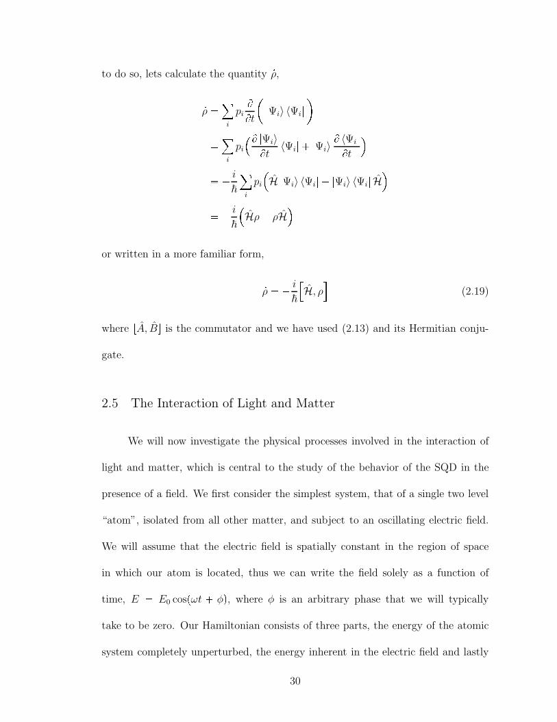
to do so, lets calculate the quantity 9ρ,9ρ i
piBBt |Ψi〉 〈Ψi|
i
pi
B |Ψi〉Bt 〈Ψi| |Ψi〉B 〈Ψi|Bt i
~i
pi
H |Ψi〉 〈Ψi| |Ψi〉 〈Ψi| H i
~
Hρ ρH
or written in a more familiar form,9ρ i
~
H, ρ
(2.19)
where rA, Bs is the commutator and we have used (2.13) and its Hermitian conju-
gate.
2.5 The Interaction of Light and Matter
We will now investigate the physical processes involved in the interaction of
light and matter, which is central to the study of the behavior of the SQD in the
presence of a field. We first consider the simplest system, that of a single two level
“atom”, isolated from all other matter, and subject to an oscillating electric field.
We will assume that the electric field is spatially constant in the region of space
in which our atom is located, thus we can write the field solely as a function of
time, E E0 cospωt φq, where φ is an arbitrary phase that we will typically
take to be zero. Our Hamiltonian consists of three parts, the energy of the atomic
system completely unperturbed, the energy inherent in the electric field and lastly
30
the interaction energy between the two. So we can write this as
H Hatom Hlight Hint . (2.20)
For our two level atomic system, we assume the energy levels of interest to be
~ωground and ~ωexcited. Since only differences in energy are of interest, we can take
the ground state energy to be zero, then the energy of the excited state relative to
the ground is ~ω0 ~pωexcited ωgroundq. Thus, in the number basis, defined by the
population of the ground and excited states, t|g〉 , |e〉u, we can write Hatom as
Hatom ~ω0a:a , (2.21)
where a is the excited state annihilation operator, and conversely, a: is the creationoperator. In reality, an atom will have many more energy levels than two. However,
as long as the frequency of the driving electric field that we consider is close to the
spacing between these two levels, then all other energy levels will be far detuned
and we will populate only these two levels. In this case, ignoring all other atomic
levels is a reasonable approximation.
We next consider the photon energy term, Hlight. Throughout this thesis, the
effect of this term is ignored. This study is focused on the large photon limit, where
the electric field can be modeled as a classical field. Including this term would
require quantizing the electric field and its coupling to the emitters. However, the
goal of this project was to fully explore the regimes of behavior possible in MNP-
SQD hybrid structures when in the classical limit for the field. We treat electric
fields classically, while treating the atom as a quantum system. This is called a
semiclassical approximation, and we make use of it throughout this thesis.
31
Lastly, we look at the interaction term of the Hamiltonian, Hint. In systems
that we are most concerned with, the typical size of our atoms, whether true atoms
or effective atomic systems (quantum dots, dyes, etc), will be much smaller than the
wavelength of light we will be concerned with ( 100 1000nm). In such a case,
we can make use of the dipole approximation for our interaction term. The classical
expression for the energy of a dipole, with dipole moment µ, in an electric field E,
is just
Eclassical µ E (2.22)
In our case, we do not have a permanent dipole but rather a neutral atom that
can undergo a dipole transition. Thus to arrive at a quantum mechanical version
of (2.22), we replace µ with the dipole operator µ [48]. In the position basis, the
dipole operator is just µ q r, where r is the usual position operator and q is the
charge.
We now need to calculate µ in the number basis. First consider 〈g| µ |g〉and 〈e| µ |e〉. For systems, such as atoms or spherical quantum dots, the energy
eigenvectors, written as |g〉 and |e〉, are either even or odd functions of their spatial
coordinates, and thus have definite parity. However, since µ has odd parity, these
diagonal matrix elements must be zero. For the other two matrix elements we
set µge 〈g| µ |e〉 and note that µeg µge. Thus we can write the matrix
representation of µ in the t|g〉 , |e〉u basis as,µ 0 µge
µge 0
ÆÆ . (2.23)
32
Since the annihilation operator has the matrix representation p 0 10 0 q, we can write
this as
µ µgea µge
a: µgea h.c., (2.24)
and we can now write Hint as
Hint pµge Eq a pµge
Eq a:. (2.25)
Now, we wish to diagonalize our Hamiltonian in the semiclassical approxima-
tion, H Hatom Hint. We take E E0 cosωt z as the form of our driving field,
where z is the unit vector in the z-direction, and set pµgeqz µ We then calculate
Hint as
Hint µE0 cosωt a µE0 cosωt a: µE0
2
eiωt eiωt
a h.c. ~ Ω
eiωt eiωt
a h.c.,
where we have defined Ω µE0
2~, which will be shown to be the usual Rabi frequency.
We now switch over to work in the interaction picture. In the interaction
picture, we transform all of our operators such that
AS Ñ Aintptq eiHatomt~ AS eiHatomt~
where we have used an S subscript to denote the operator in the Schrodinger picture.
Because Hatom commutes with eiHatomt~, it takes the same form in both pictures,
33
however Hint is now
Hint ~ Ωeiωt eiωt
eiω0a
:SaSt aS e
iω0a:SaSt h.c. ~ Ω
eiωt eiωt
eiω0t aS h.c. ~ Ω
eipωω0qt eipωω0qt aS h.c.
where we have used the relation eiω0a:SaSt aS e
iω0a:SaSt eiω0t aS. Near resonance,
we can assume pω ω0q ¡¡ pω ω0q. Therefore, the eipωω0qt terms, will oscillate
much faster than the eipωω0qt terms. Thus on the time scales that we are interested
in, t 2πpωω0q , the effect of the fast oscillating term averages to zero and can be
neglected. This is the rotating wave approximation. Dropping these terms and
moving back to the Schrodinger picture, our interaction Hamiltonian is,
Hint ~ Ω eiωt a ~ Ω eiωt a:. (2.26)
Now, we solve the master equation,9ρ i
~
Hatom Hint, ρ
. (2.27)
Working in the basis that diagonalizes Hatom, we can write down the following
differential equations for the components of ρ,9ρgg i Ω eitω ρeg i Ω eitω ρge9ρge i Ω eitω p ρee ρggq iω0ρge9ρee i Ω eitω ρge i Ω eitω ρeg.
It is important to remember that because ρeg ρge, the equation for 9ρeg is
redundant. However, we do have an additional restraint from the normalization of
34

the density matrix, ρeeρgg 1. The factors of eitω paired with ρge, as well as the
iω0ρge term in the equation for 9ρge suggests a solution of the form ρgeptq rρgeptq eiωt,where we have explicitly factored out the fast oscillating component of ρge by moving
to a rotating frame. Our equations are now,9ρgg i Ω rρ ge i Ω rρge9rρge i Ω p ρee ρggq i pω0 ωq rρge9ρee i Ω rρge i Ω rρ
ge .
Now, let rρge A iB and Ω ΩR i ΩI , and also define ∆ge ρgg ρee. Then
we have, 9∆ge 4 ΩI A 4 ΩR B9A pω ω0q B ΩI ∆ge (2.28)9B pω ω0q A ΩR ∆ge .
The first equation is the result of taking the difference of the first and third equations
of the previous set of equations.
We can solve these equations for the steady state solution by taking the left
hand side of (2.28) to be zero and solving the resulting homogeneous system of
equations. However, this set of equations for the steady state limit, as a system of
linear homogeneous equations will have either only the null solution (i.e., A B ∆ge 0), or, the null solution along with infinitely more solutions. Thus this model
is rather unphysical. In order to make our model more accurate, we need to discuss
spontaneous and stimulated emission, which evidently must be present in any real
35
physical system.
2.6 Stimulated and Spontaneous Emission
As shown in the previous section, an electric field can cause transitions in an
atom system. It also turns out to be true even in the absence of an applied electric
field. This is due to the fact that the atom can emit into the vacuum modes of the
electric field. This interaction with the vacuum (as well as any noise that is also
present) can be modeled by assuming that our atomic system is also interacting
with a reservoir.
Consider the situation in which our (atomic) system is in contact with a reser-
voir which we call the “bath”. The bath may simply be the vacuum fluctuations
of the electric field, or a particularly noisy mode that can induce transitions in our
system. Regardless of the origin of the bath, we first make a few assumptions about
the nature of the bath.
(a) The bath is much larger than the system of interest, i.e., the bath is much
more influential on our system, than our system is on the bath. Thus we take
the statistical properties of the bath to be unaffected by the interaction with
the system.
(b) The bath and our system are weakly correlated (or more precisely, the coher-
ence between the bath and system can be neglected). From this assumption,
we mean that the density matrix describing the combination of the bath and
our system can be factored and we can write ρtotal ρB b ρS.
36
(c) The bath has no memory. Thus the interaction between our system and the
bath is a Markov process, i.e., the future evolution of bath is not dependent
on the past configuration of the bath. Since “memory” in the quantum sense
is given by correlation functions, this means that the correlation time of the
bath is much shorter than the time scales that we are interested in for our
system.
We begin our analysis by writing the Hamiltonian for the combined system,
H HB HS Hint (2.29)
where the B subscript denotes the bath, S denotes our system and “int” is the
interaction between the two. We denote the density matrix for the combined system
as ρtotal, and now move to the interaction picture and write
ρIptq eipHSHBq~ ρtotal eipHSHBq~HIptq eipHSHBq~ Hint e
ipHSHBq~where HIptq is the interaction Hamiltonian in the interaction picture. The density
matrix and Hamiltonian must satisfy the relation9ρIptq i
~rHIptq, ρIptqs . (2.30)
Integrating equation (2.30) from 0 to t, we have
ρIptq ρIp0q i
~
» t
0
dt1rHIpt1q, ρIpt1qs . (2.31)
We now iterate this equation for ρIptq by taking tÑ t1 and t1 Ñ t2 and substituting
37
for ρIpt1q on the RHS of (2.31) which gives us,
ρIptq ρIp0q i
~
» t
0
dt1rHIpt1q, ρIp0qs 1
~2
» t
0
dt1 » t10
dt2rHIpt1q, rHIpt2q, ρIpt2qss .Finally, differentiating with respect to t, we arrive at9ρIptq i
~rHIptq, ρIp0qs 1
~2
» t
0
dτ rHIptq, rHIpτq, ρIpτqss , (2.32)
where the integration variable t2 has been renamed as τ .
We pause here for a moment to recall that ρtot and ρIptq are operators on the
combined space of the bath and system variables. This is not a very useful quantity.
The quantity we are actually interested in finding is the reduced density matrix
which is obtained by taking ρtot and tracing over the bath variables,rρtotal TrBrρtotals . (2.33)
We similarly define the reduced interaction picture density matrixrρIptq TrBrρIptqs . (2.34)
Now, performing a trace over the bath variables on both sides of (2.32), we
have,9rρIptq i
~TrB
rHIptq, ρIp0qs 1
~2
» t
0
dτ TrB
rHIptq, rHIpτq, ρIpτqss . (2.35)
First, we assume that initially, the bath and system are uncorrelated. Thus, ρIp0q ρtotalp0q ρB b ρSp0q. Next, consider the first term. We can assume that this term
is zero if Hint has no diagonal elements over the bath variables (i.e., Hint always
38
changes the bath quantum numbers). Although there is no reason to expect that
Hint will not contain any terms with factors of b:b, for example, we assume that
we can do so with a suitable redefinition of Hsys and Hint. By now invoking our
assumption that the bath is relatively unchanged by the interaction with the system,
we can approximate the interaction picture density matrix as the tensor product of
the bath density matrix and the reduced interaction picture density matrix,
ρIptq ρB b rρIptq . (2.36)
These approximations now allow us to write (2.35) as9rρIptq 1
~2
» t
0
dτ TrB
rHIptq, rHIpt τq, ρB b rρIpt τqss . (2.37)
where we have also made the change in integration variable τ Ñ t τ .
Lastly, we invoke the Markov approximation which allows us to assume that
over the time scale of the bath correlation time, rρIptq is relatively unchanged com-
pared to the bath variables. This allows us to take rρIpt τq rρIptq. Furthermore,
if we assume that t is much larger than the bath correlation time, then we can time
the limit of our integral to infinity and we can write (2.37) now in its usual form
[49], 9rρIptq 1
~2
» 80
dτ TrB
rHIptq, rHIpt τq, ρB b rρIptqss , (2.38)
which is a first order differential equation in time, showing the Markovian property
of the combined system.
39
2.7 Toy Model: Two Level System Interacting with a Single Bosonic
Mode
We now use the formalism we just developed to model the spontaneous emis-
sion from an atomic system. We again consider a two level atom, but now we allow
the atom to interact with a bath consisting of a single bosonic mode. We begin with
the following Hamiltonians,
HS ~ωss:s
HB ~ωbb:b
Hint µs:b b:s
where s: and s are the (fermionic) raising and lowering operators for the atomic
system, and b: and b are the (bosonic) raising and lowering operators for the bath.
Then 9rρIptq 1
~2
» 80
dτ TrB
rHIptq, rHIpt τq, ρB b rρIptqss 1
~2
» 80
dτB
〈B| HIptq HIpt τq ρB b rρIptq |B〉 〈B| HIptq ρB b rρIptq HIpt τq |B〉 〈B| HIpt τq ρB b rρIptq HIptq |B〉 〈B| ρB b rρIptq HIpt τq HIptq |B〉
1
~2
» 80
dτ p T1 T2 T3 T4 q . (2.39)
40
We now evaluate each term in turn.
T1 B
〈B| HIptq HIpt τq ρB b rρIptq |B〉µB
eipHSEBqt~ s: ?B 1 〈B 1| s?B 〈B 1| eipHSHBqτ~ Hint e
ipHSHBqptτq~ ρB b rρIptq |B〉µB
eiBωbt
eiωbpB1qτ eiωst s: eiHSτ~ ?B 1 〈B 1| eiωbpB1qτ s eiHSτ~ ?B 〈B 1| Hint e
ipHSHBqptτq~ ρB b rρIptq |B〉
T1 µ2
B
eiBωbptτqeiωbτ eiωst s: ?B 1 〈B 1| eiωbτ eiωsτ s?B 〈B 1| s:b b:s eipHSHBqptτq~ ρB b rρIptq |B〉µ2
B
eiBωbptτqeiωbτ eiωst s: s pB 1q eiωbτ eiωsτ s s: B 〈B| eipHSHBqptτq~ ρB b rρIptq |B〉µ2
B
eiωbτ eiωsτ s: s pB 1q eiωbτ eiωsτ s s: B 〈B|ρB |B〉b rρIptqµ2
eiωbτ eiωsτ
sB 1s: s rρIptq eiωbτ eiωsτ sB s s: rρIptq
where we have repeatedly used identities like s eα s:s eαs and eα s:s s s, and
we have used sB to denote the average population of the bosonic mode, sB °B 〈B|ρB |B〉.
41
Now turning our attention to T2,
T2 B
〈B| HIptq ρB b rρIptq HIpt τq |B〉 µ2
B
eiBωbt
eiωst eipB1qωbt s: ?B 1 〈B 1| eiωst eipB1qωbt s
?B 〈B 1| ρB b rρIptqeiωsptτq eipB1qωbptτq s:?B |B 1〉 eiωsptτq eipB1qωbptτq s?B 1 |B 1〉
eiBωbptτq µ2
eiωsτ eiωbτ sB s: rρIptq s eiωsτ eiωbτ p sB 1q s rρIptq s:
where we have we have used that°
B B 〈B 1| ρB |B 1〉 sB 1. Also, we have
assumed that terms like°
B 〈B 1| ρB |B 1〉 can be taken to be zero, which is a
safe assumption if our bath is in a thermal state (i.e. has no correlation). However,
this would not hold if our bath was in a squeezed state. The calculation for T3 is
similar,
T3 B
〈B| HIpt τq ρB b rρIptq HIptq |B〉 µ2
B
eiBωbptτqeiωsptτq eipB1qωbptτq s: ?B 1 〈B 1| eiωsptτq eipB1qωbptτq s ?B 〈B 1| ρB b rρIptqeiωst eipB1qωbt s:?B |B 1〉 eiωst eipB1qωbt s?B 1 |B 1〉
eiBωbt µ2
eiωsτ eiωbτ sB s: rρIptq s eiωsτ eiωbτ p sB 1q s rρIptq s: .
42
Lastly, a calculation for T4 yields,
T4 B
〈B| ρB b rρIptq HIpt τq HIptq |B〉µ2
eiωsτ eiωbτ sB rρIptq s s: eiωsτ eiωbτ p sB 1q rρIptq s: s .
Returning to (2.39) and putting this together,9rρIptq 1
~2
» 80
dτ p T1 T2 T3 T4 q µ2
~2
» 80
dτ
eiωbτ eiωsτ sB s s: rρIptq eiωbτ eiωsτ
sB 1s: s rρIptq eiωsτ eiωbτ sB s: rρIptq s eiωsτ eiωbτ p sB 1q s rρIptq s: eiωsτ eiωbτ sB s: rρIptq s eiωsτ eiωbτ p sB 1q s rρIptq s: eiωsτ eiωbτ sB rρIptq s s: eiωsτ eiωbτ p sB 1q rρIptq s: s µ2
~2
» 80
dτ
eipωbωsqτ sB s s: rρIptq s: rρIptq s eipωbωsqτ sB rρIptq s s: s: rρIptq s eipωbωsqτ p sB 1q rρIptq s: s s rρIptq s: eipωbωsqτ p sB 1q s: s rρIptq s rρIptq s: γ sB s s: rρIptq rρIptq s s: 2 s: rρIptq s γ p sB 1q s: s rρIptq rρIptq s: s 2 s rρIptq s: i ǫ sB r s s:, rρIptqs i ǫ p sB 1q r s: s, rρIptqs
where we have defined µ2
~2
³80dτeipωbωsqτ γ iǫ. The terms proportional to ǫ sB
and ǫ p sB1q are the Stark and Lamb shifts respectively. They represent small shifts
in the energy levels of the system and can often be neglected. The term proportional
43
to γ p sBq goes to zero as the average excitation population of the bath goes to zero,
and thus would not be present at zero temperature. However, the γp sB 1q termis present even at zero temperature and represents transitions in our system from a
state with a higher energy to a lower energy state, while the previous must represent
a transition from a lower energy state to one that is higher.
2.8 Lindblad Master Equation
In this thesis, we will model interactions at optical frequencies. We can further
develop our framework of modeling open systems in such a case. To do so, we return
to the case of an atomic system in an arbitrary bath, at optical frequencies. We
assume only that our interaction Hamiltonian can be written as
Hint ~
j
s:j bj sj b
:j
(2.40)
where the bj are some set of bath operators, and the sj are operators on the system
Hilbert space and satisfy rHsys, sjs ~ωj sj . (2.41)
For example, interaction terms with s a, where a is an annihilation operator
would represent an excitation transfer with the bath. Additionally, terms where
s a:a (noting that rHsys, a:as 0 trivially satisfies (2.41)) would be indicative of
bath induced scattering processes and would give rise to dephasing in our system.
From (2.41) we can work out the following identity that will be very useful in
44
the derivation that follows. Consider the quantity, eαHsys sj,
eαHsys sj 1 α Hsys 1
2!pα Hsysq2 . . .
sj
sj sj αp Hsys ~ωjq sj1
2!
αp Hsys ~ωjq2 . . .
sj eαpHsys~ωjq .
Thus, in the interaction picture,
sjptq eiHsyst~ sj eiHsyst~ eiωjt sj (2.42)
and similarly,
s:jptq eiHsyst~ sj eiHsyst~ eiωjt s:j . (2.43)
Now, we return our attention to (2.40) and substitute this interaction Hamil-
tonian into (2.38), our master equation for the reduced density matrix. We again
have many terms to evaluate and define T1, T2, T3, and T4 as before. Thus,
T1 1
~2TrBr HIptq HIpt τq ρB b rρIptqs
j k
TrB
eiωjt s
:j bjptq eiωjt sj b
:jptq eiωkptτq s:k bkpt τq eiωkptτq sk b:kpt τq ρB b rρIptq
j k
TrB
eiωjτ eipωjωkqt s:j sk bjptq b:kpt τq eiωjτ eipωjωkqt sj s:k b:jptq bkpt τq ρB b rρIptq ,
45

where we have again dropped terms like TrBr bjptq bkpt τq ρBs, assuming that
our bath is in a thermal state. We now make the rotating wave approximation by
neglecting terms with j k. We can do so because if ωj ωk, then eipωjωkqt isa quickly varying function over the time scale of the correlation time, and thus will
make only a minor contribution compared to the term with j k. However, if j
and k are degenerate energy eigenstates, then this would not hold and care would
need to be taken. Returning to T1, we have
T1 j
eiωjτ TrB
bjptq b:jpt τq ρB s:j sj rρIptq eiωjτ TrB
b:jptq bjpt τq ρB sj s:j rρIptq
Proceeding to T2, we find,
T2 j
eiωjτ TrB
bjptq ρB b
:jpt τq s:j rρIptq sj eiωjτ TrB
b:jptq ρB bjpt τq sj rρIptq s:j
j
eiωjτ TrB
b:jpt τq bjptq ρB s:j rρIptq sj eiωjτ TrB
bjpt τq b:jptq ρB sj rρIptq s:j,
where we have used the cyclic property of the trace. Similarly for T3 and T4 we
46
have,
T3 j
eiωjτ TrB
b:jptq bjpt τq ρB s:j rρIptq sj eiωjτ TrBbjptq b:jpt τq ρB sj rρIptq s:j
T4 j
eiωjτ TrB
bjpt τq b:jptq ρB rρIptq s:j sj eiωjτ TrBb:jpt τq bjptq ρB rρIptq sj s:j .
We now make the Markov approximation and assume that factors like
TrBbjpt τq b:jptq ρB
are functions of τ only as the bath has very short memory. This allows us to write
this factor as TrBbjp0q b:jpτq ρB. Upon transforming all of the terms we’ve
accumulated, our correlation factors all take one of four possible forms,
eiωjτ TrBb:jpτq bjp0q ρB
eiωjτ TrBb:jp0q bjpτq ρB
eiωjτ TrBbjp0q b:jpτq ρB
eiωjτ TrBbjpτq b:jp0q ρB .
Noting that the first two of these terms are complex conjugates of each other, and
that the same can be said for the third and fourth terms, we make the following
47

definitions, » t
0
dτ eiωjτ TrBb:jp0q bjpτq ρB Γj iǫj» t
0
dτ eiωjτ TrBb:jpτq bjp0q ρB Γj iǫj» t
0
dτ eiωjτ TrBbjpτq b:jp0q ρB γj iδj» t
0
dτ eiωjτ TrBbjp0q b:jpτq ρB γj iδj .
If the bj are creation operators, then at zero temperature both γ and δ are non zero
due to the ordering of bjpτq and b:jpτq, and are thus the result of vacuum fluctuations.
Now returning to our master equation,9rρIptq 1
~2
» t
0
dτ p T1 T2 T3 T4 q j
pγj iδjq s:j sj rρIptq pΓj iǫjq sj s:j rρIptq pΓj iǫjq s:j rρIptq sj pγj iδjq sj rρIptq s:j pΓj iǫjq s:j rρIptq sj pγj iδjq sj rρIptq s:j pγj iδjq rρIptq s:j sj pΓj iǫjq rρIptq sj s:j j
"γjs:j sj rρIptq rρIptq s:j sj 2sj rρIptq s:j Γj
sj s
:j rρIptq rρIptq sj s:j 2s:j rρIptq sj iδj
s:j sj rρIptq rρIptq s:j sj iǫj
rρIptq sj s:j sj s:j rρIptq * .
We again identify ǫj and δj as the Lamb and Stark shifts, and note that they play
little role in the analysis that follows and will be neglected from here on out.
48
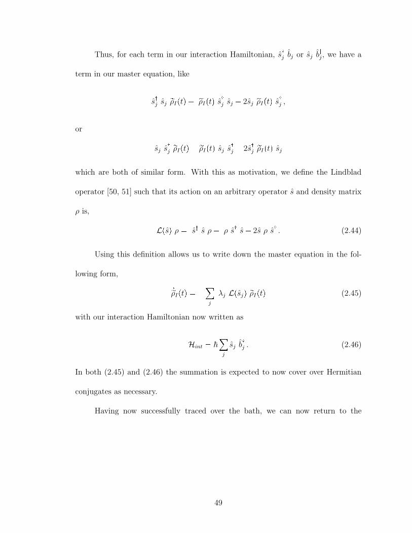
Thus, for each term in our interaction Hamiltonian, s:j bj or sj b:j , we have a
term in our master equation, like
s:j sj rρIptq rρIptq s:j sj 2sj rρIptq s:j ,
or
sj s:j rρIptq rρIptq sj s:j 2s:j rρIptq sj
which are both of similar form. With this as motivation, we define the Lindblad
operator [50, 51] such that its action on an arbitrary operator s and density matrix
ρ is,
Lpsq ρ s: s ρ ρ s: s 2s ρ s: . (2.44)
Using this definition allows us to write down the master equation in the fol-
lowing form, 9rρIptq j
λj Lpsjq rρIptq (2.45)
with our interaction Hamiltonian now written as
Hint ~
j
sj b:j . (2.46)
In both (2.45) and (2.46) the summation is expected to now cover over Hermitian
conjugates as necessary.
Having now successfully traced over the bath, we can now return to the
49
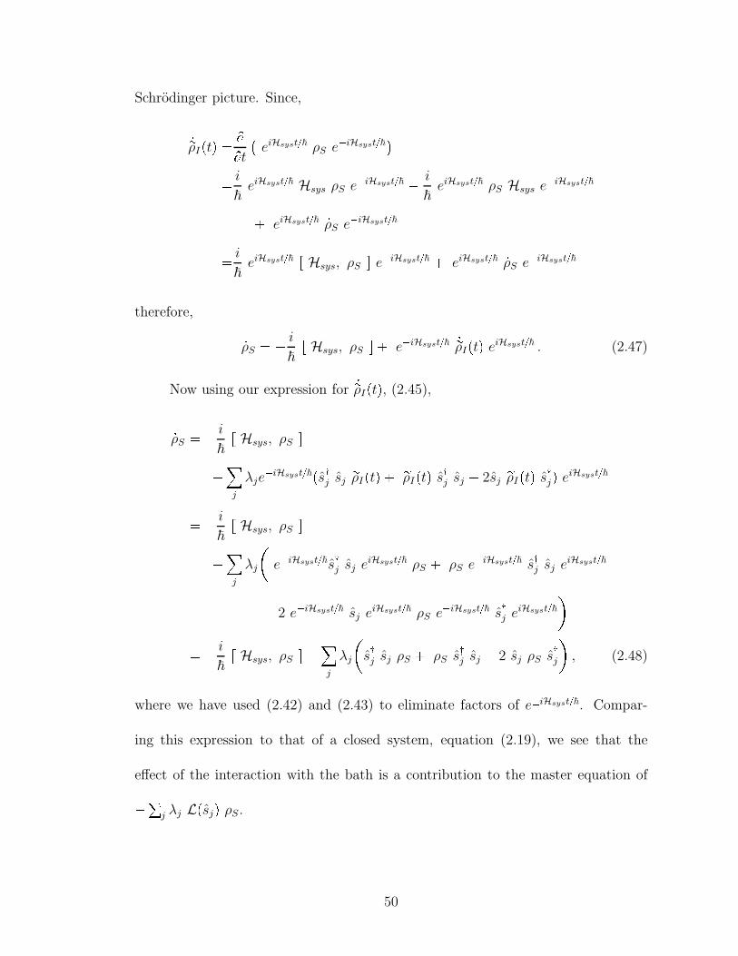
Schrodinger picture. Since,9rρIptq BBt eiHsyst~ ρS eiHsyst~ i
~eiHsyst~ Hsys ρS e
iHsyst~ i
~eiHsyst~ ρS Hsys e
iHsyst~ eiHsyst~ 9ρS eiHsyst~ i
~eiHsyst~ r Hsys, ρS s eiHsyst~ eiHsyst~ 9ρS eiHsyst~
therefore, 9ρS i
~r Hsys, ρS s eiHsyst~ 9rρIptq eiHsyst~ . (2.47)
Now using our expression for 9rρIptq, (2.45),9ρS i
~r Hsys, ρS sj
λjeiHsyst~ps:j sj rρIptq rρIptq s:j sj 2sj rρIptq s:jq eiHsyst~ i
~r Hsys, ρS sj
λj
eiHsyst~s:j sj eiHsyst~ ρS ρS e
iHsyst~ s:j sj eiHsyst~ 2 eiHsyst~ sj eiHsyst~ ρS eiHsyst~ s:j eiHsyst~ i
~r Hsys, ρS s
j
λj
s:j sj ρS ρS s
:j sj 2 sj ρS s
:j
, (2.48)
where we have used (2.42) and (2.43) to eliminate factors of eiHsyst~. Compar-
ing this expression to that of a closed system, equation (2.19), we see that the
effect of the interaction with the bath is a contribution to the master equation of°j λj Lpsjq ρS.50
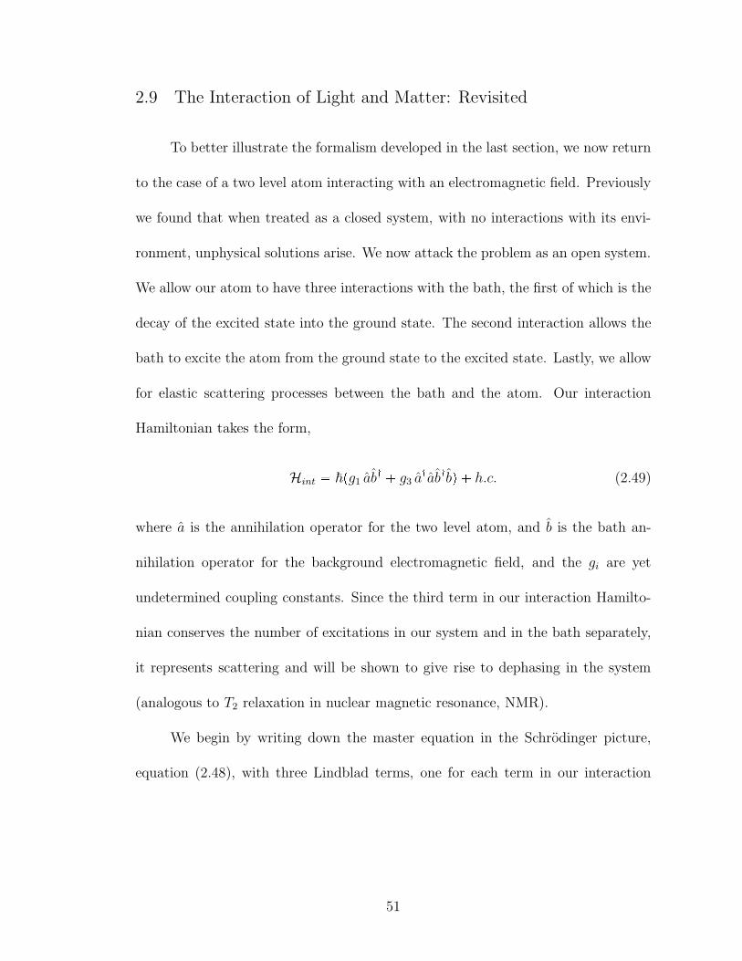
2.9 The Interaction of Light and Matter: Revisited
To better illustrate the formalism developed in the last section, we now return
to the case of a two level atom interacting with an electromagnetic field. Previously
we found that when treated as a closed system, with no interactions with its envi-
ronment, unphysical solutions arise. We now attack the problem as an open system.
We allow our atom to have three interactions with the bath, the first of which is the
decay of the excited state into the ground state. The second interaction allows the
bath to excite the atom from the ground state to the excited state. Lastly, we allow
for elastic scattering processes between the bath and the atom. Our interaction
Hamiltonian takes the form,
Hint ~pg1 ab: g3 a:ab:bq h.c. (2.49)
where a is the annihilation operator for the two level atom, and b is the bath an-
nihilation operator for the background electromagnetic field, and the gi are yet
undetermined coupling constants. Since the third term in our interaction Hamilto-
nian conserves the number of excitations in our system and in the bath separately,
it represents scattering and will be shown to give rise to dephasing in the system
(analogous to T2 relaxation in nuclear magnetic resonance, NMR).
We begin by writing down the master equation in the Schrodinger picture,
equation (2.48), with three Lindblad terms, one for each term in our interaction
51
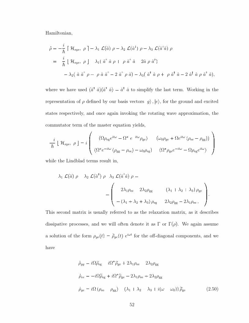
Hamiltonian,9ρ i
~r Hsys, ρ s λ1 Lpaq ρ λ2 Lpa:q ρ λ3 Lpa:aq ρ i
~r Hsys, ρ s λ1p a: a ρ ρ a: a 2a ρ a:q λ2p a a: ρ ρ a a: 2 a: ρ aq λ3p a: a ρ ρ a: a 2 a: a ρ a: aq,
where we have used pa: aqpa: aq a: a to simplify the last term. Working in the
representation of ρ defined by our basis vectors |g〉 , |e〉, for the ground and excited
states respectively, and once again invoking the rotating wave approximation, the
commutator term of the master equation yields,i~
r Hsys, ρ s i
pΩρegeitω Ω eitωρgeq pω0ρge Ωeitω pρee ρggqqpΩeitω pρgg ρeeq ω0ρegq pΩρgeeitω Ωρegeitωq ÆÆ
while the Lindblad terms result in,λ1 Lpaq ρ λ2 Lpa:q ρλ3 Lpa:aq ρ 2λ1ρee 2λ2ρgg pλ1 λ2 λ3q ρgepλ1 λ2 λ3q ρeg 2λ2ρgg 2λ1ρee ,
ÆÆ .This second matrix is usually referred to as the relaxation matrix, as it describes
dissipative processes, and we will often denote it as Γ or Γpρq. We again assume
a solution of the form ρgeptq rρgeptq eiωt for the off-diagonal components, and we
have 9ρgg iΩrρeg iΩrρge 2λ1ρee 2λ2ρgg9ρee iΩrρeg iΩrρge 2λ1ρee 2λ2ρgg9ρge iΩ pρee ρggq pλ1 λ2 λ3 ipω ω0qq rρge (2.50)
52
We now examine (2.50) in the absence of a driving field (Ω Ñ 0), and in the
steady state limit ( 9ρ Ñ 0). By taking the difference of the first two equations, we
have
λ1ρpeqqee λ2ρ
peqqgg , (2.51)
where the peqq superscript is to remind us that this is really an equilibrium equation.
However, if the system is in equilibrium at some temperature, T , the ratio NeNg,
can also be calculated from the Boltzmann factor as NeNg e~ω0kBT . Thus we
must have,
λ2
λ1 e~ω0kBT . (2.52)
We see here, as was mentioned in the previous section, that as T Ñ 8, λ2 Ñ 0. λ2
arises from an interaction Hamiltonian term of the form a: b, i.e. excitation from
the bath. At optical frequencies ~ω0 1eV, and thus even at room temperature,
kBT 140, this factor is vanishingly small and λ2 can be taken to be zero.
Returning to (2.50) in the general case, we make the following definitions, let
1τ 2λ1 and 1
T pλ1 λ3q, and as before define ∆ge ρgg ρee. Now, we have,9∆ge 2iΩrρeg 2iΩrρge ∆ge 1
τ9rρge 1
T i pω ω0q rρge iΩ∆ge ,
or working in components, rρge A iB, and assuming that Ω is real,9∆ge 4 Ω B ∆ge 1
τ9A pω ω0q B A
T9B pω ω0q A Ω ∆ge B
T. (2.53)
53
We can solve these equations for the steady state solution by taking the LHS of
(2.53) to be zero, and with some straightforward algebra we find,
∆ge T 2 pω ω0q 2 1
T 2 pω ω0q 2 4τTΩ2 1
B Ω ∆ge
T
1T 2 pω ω0q2
A pω ω0qΩ∆ge
1T 2 pω ω0q2 .
When ρ is viewed as a function of ω, the driving field frequency, we see that both B
and ∆ge are peaked at ω ω0 while A changes sign here. This is the resonance con-
dition for the system and comparing these expressions to the well known Lorentzian
line shape function, T is evidently the half-width at half-maximum.
We now solve (2.53) in the case where the driving field is on resonance with
the atomic transition, so ω ω0,9∆ge 4 Ω B ∆ge 1
τ9A AT9B Ω ∆ge B
T. (2.54)
In this case A becomes uncoupled from the other components and we can solve for
it immediately,
Aptq Ap0qetT .We see that an effect of the elastic scattering interaction with the bath is to cause an
exponential decay in the real component of the off-diagonal density matrix element.
Since this a measurement of the quantum mixing of the ground and excited states,
54
then this is indicative of the system losing quantum coherence, i.e. we can say that
T leads to decoherence as a pure state will decay into a mixed state at a rate of 1T.
Although (2.54) can be solved for B and ∆ge in closed form, the solutions are
not very instructive. Instead, we examine the solution in two limits, namely that of
a strong field Ω ¡¡ τ, T and a weak field Ω τ, T . In the weak field limit, we
neglect the 4 Ω B and Ω ∆ge terms and we find
∆geptq ∆gep0qetτBptq Bp0qetT .
Here, because the damping is so much larger than the driving field, the system no
longer has the opportunity to oscillate, and B and ∆ge exponentially decay to zero.
We say that the system in overdamped.
In strong field limit, we instead neglect the terms ∆ge1
τand B
Tin (2.54), and
take |g〉 to be the initial state our system is prepared in, and find,
∆geptq cos p2ΩtqBptq 1
2sin p2Ωtq .
Here we see that B and ∆ge oscillate at the frequency 2Ω, which is twice the Rabi
frequency (we could have equivalently chosen Ω µE
~instead of Ω µE
2~). In
particular, ∆ge alternates between the values of 0 and 1, which implies that the
system oscillates between being fully in the ground state (∆ge 1) and fully in the
excited state (∆ge 1), and between these points, in a 5050 split between the
ground and excited state (∆ge 0). At the times when ∆ge 0, B takes on its
55
maximal/minimal value of 12which implies that the system is in a pure state which
is consistent with the relaxation terms in (2.54) being ignored. As these oscillations
would continue ad infinitum, we say that the system is underdamped in this limit.
In chapter 3, we will model the response of an SQD (an effective two level
system), in the presence of an MNP and an applied driving field, both of which will
act as a source of electromagnetic radiation incident on the SQD. There, we will see
that many features of this simple model will appear with only slight modification
when we model SQD-MNP system.
2.10 Computational Technique
We finish this chapter with a few words on how calculations performed for
this research were carried out. First, choices are made for the various system pa-
rameters. The next step is to calculate, either with a dipole approximation, or with
the BEM, the response fields of the MNP, at the location of the SQD. With these
fields, along with the Lindblad terms included to model losses, we can write down
a master equation for the SQD. This set of coupled differential equations is then
solved numerically using Mathematica, usually in both the dynamical limit, as well
as the steady state limit. Once these equations are solved, and ρSQD is found in the
desired limit, observable quantities, such as the absorption, can then be calculated.
By then varying the parameters that we are free to choose while repeatedly solving
the master equation, the system behavior can be fully explored.
56
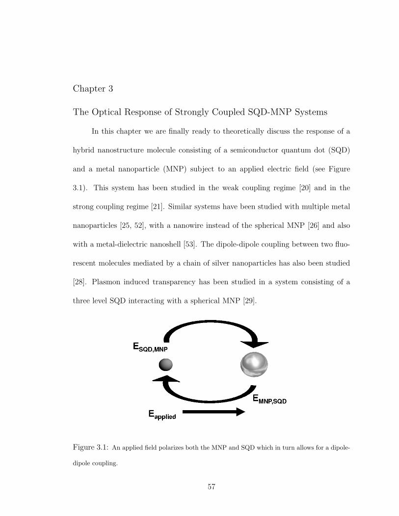
Chapter 3
The Optical Response of Strongly Coupled SQD-MNP Systems
In this chapter we are finally ready to theoretically discuss the response of a
hybrid nanostructure molecule consisting of a semiconductor quantum dot (SQD)
and a metal nanoparticle (MNP) subject to an applied electric field (see Figure
3.1). This system has been studied in the weak coupling regime [20] and in the
strong coupling regime [21]. Similar systems have been studied with multiple metal
nanoparticles [25, 52], with a nanowire instead of the spherical MNP [26] and also
with a metal-dielectric nanoshell [53]. The dipole-dipole coupling between two fluo-
rescent molecules mediated by a chain of silver nanoparticles has also been studied
[28]. Plasmon induced transparency has been studied in a system consisting of a
three level SQD interacting with a spherical MNP [29].
Figure 3.1: An applied field polarizes both the MNP and SQD which in turn allows for a dipole-
dipole coupling.
57
3.1 Introduction
The optical excitations of the SQD are the excitons, with a sharp, discrete
response. The SQD acts as a quantum emitter. The strong local plasmonic excita-
tions of the MNP offer a continuous spectrum of response. Local field enhancement
in the vicinity of the MNP should provide strong coupling to the neighboring SQD.
There is no direct tunneling of charge carriers between the MNP and SQD. However,
due to the long-range Coulomb interaction, there is a dipole-dipole interaction that
will allow them to couple and will lead to excitation transfer.
The discrete excitons coupled with the broad response of the plasmons should
allow for the appearance of exotic hybrid states and clear signatures for their optical
response. We will see that as a damped driven oscillator, the SQD response to
driving fields changes rapidly from in-phase to out-of-phase near the SQD resonance.
Rapid variations in hybrid response are expected near the SQD resonance. Effects
depending on the interference between applied and induced fields are extremely
sensitive to this change from in-phase to out-of-phase SQD response, providing
dramatic signatures from the hybrid response.
Previously, the weak coupling regime was studied in [20]. In the weak field/weak
coupling limit (driving field of 1W/cm2), a shift and broadening of the peak in the
energy absorption spectrum due to the coupling between the exciton in the SQD
and the plasmon in the MNP was found. In the strong field/weak coupling limit,
an asymmetrical Fano shape, develops in the energy absorption spectrum.
Here, we will examine the strong coupling regimes, in particular probing fur-
58
ther the strong applied field limit. We find that the behavior is much more complex
than previously determined [20]. When we explore the relationship between the
size of the constituents and the response of the system, we find that in addition to
the regime for weak coupling which was previously explored, there are three new
regimes of system behavior in the strong coupling limit. These four (in total) dis-
tinct regimes of behavior in the strong field limit each exhibit novel properties and
we will look at each.
In the first regime the energy absorption spectrum displays an asymmetrical
Fano shape (as previously predicted in [20]). It occurs when there is interference
between the applied field and the induced field produced by the SQD at the MNP. As
the SQD is increased in size (thus the coupling is increased), the asymmetrical Fano
effect of region I is modified by the appearance of an additional peak with a deep
minimum between the peaks [21]. Here, the induced local field at the MNP becomes
larger than the applied field, for frequencies near the SQD resonance. As such, the
interference of the the response field of the SQD, with the applied electric field, now
results in a sign change in the net electric field at the MNP above resonance where
the two fields are out-of-phase. An exciton induced transparency (EXIT) arises in
the MNP response when there is nearly complete destructive interference between
these two fields acting on the MNP.
When the MNP and SQD are further increased in size, the hybrid behavior
transitions between regions II and III. In this regime, there is a discontinuous jump
in response of the system (in both the diagonal and off-diagonal density matrix el-
ements) as the driving frequency is varied [22]. Moreover, the response of the SQD
59
is highly suppressed above resonance in this transition region. The discontinuous
response and suppression arise because the SQD acts as a driven (quantum) oscil-
lator. Below resonance the dipole moment of the SQD is in phase with the driving
field and above resonance it is 180 out of phase. The phase change at resonance
drastically alters the hybrid response when crossing the resonance.
Finally, in region III, the system response becomes nonlinear. This nonlinear-
ity is due to significant self interaction of the SQD (feedback through the MNP). In
this regime, there exists multiple steady state solutions leading to a bistability with
one of the stable solutions having a discontinuous absorption spectrum [21]. In this
chapter will explore these four regimes in detail and set bounds on each.
The layout of this chapter is as follows. In section 2, we discuss the system
in detail. We use a density matrix approach to treat the SQD, while the MNP is
taken as a classical dielectric. We also calculate the energy absorption of the MNP
and provide details on how numerical calculations were carried out. In section 3
the Fano-like behavior of the system in region I will be discussed. In section 4,
the exciton induced transparency of region II is introduced. We then discuss the
suppressed response of the SQD that occurs in the transition region, in section 5.
In section 6, we look at region III, where the system response is dominated by
nonlinear effects and bistability can occur. In section 7, we will investigate the
roll that the phasors and interaction strengths play in determining which regime
of system behavior is present. In section 8, we examine how the polarization of
the incident light effects the system behavior. Finally, a summary of findings is
presented in section 8.
60
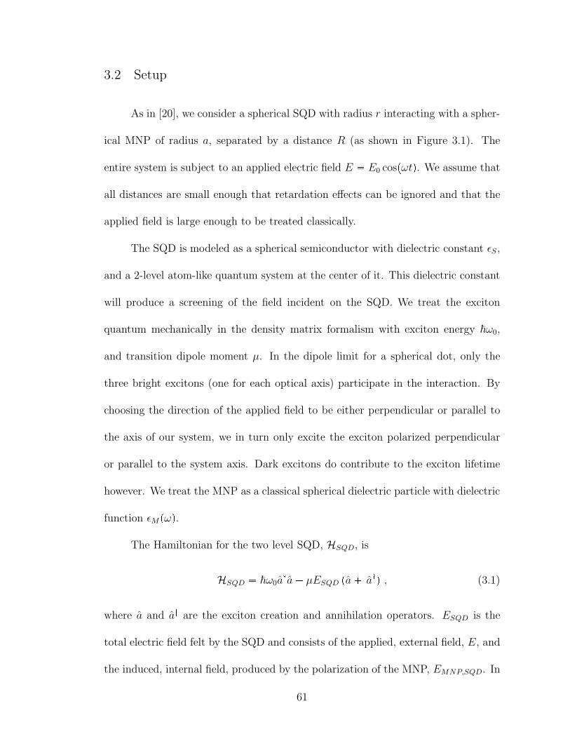
3.2 Setup
As in [20], we consider a spherical SQD with radius r interacting with a spher-
ical MNP of radius a, separated by a distance R (as shown in Figure 3.1). The
entire system is subject to an applied electric field E E0 cospωtq. We assume that
all distances are small enough that retardation effects can be ignored and that the
applied field is large enough to be treated classically.
The SQD is modeled as a spherical semiconductor with dielectric constant ǫS,
and a 2-level atom-like quantum system at the center of it. This dielectric constant
will produce a screening of the field incident on the SQD. We treat the exciton
quantum mechanically in the density matrix formalism with exciton energy ~ω0,
and transition dipole moment µ. In the dipole limit for a spherical dot, only the
three bright excitons (one for each optical axis) participate in the interaction. By
choosing the direction of the applied field to be either perpendicular or parallel to
the axis of our system, we in turn only excite the exciton polarized perpendicular
or parallel to the system axis. Dark excitons do contribute to the exciton lifetime
however. We treat the MNP as a classical spherical dielectric particle with dielectric
function ǫMpωq.The Hamiltonian for the two level SQD, HSQD, is
HSQD ~ω0a:a µESQD pa a:q , (3.1)
where a and a: are the exciton creation and annihilation operators. ESQD is the
total electric field felt by the SQD and consists of the applied, external field, E, and
the induced, internal field, produced by the polarization of the MNP, EMNP,SQD. In
61
the dipole limit, ESQD is
ESQD 1
ǫeffS
E 1
4πǫB
sαPMNP
R3
, (3.2)
where sα 2p1q when the applied field is parallel (perpendicular) to the major
axis of the system and ǫeffS 2ǫBǫS3ǫB
accounts for the screening of the dielectric
material. ǫB is a background dielectric constant which we could assume to be from
the material that our system in embedded in. Being careful to separate out the
negative and positive frequency contributions, the polarization of the MNP is (see
[54]),
PMNP p4πǫBqa3γ rEpqMNP eiωt γ rEpq
MNP eiωt.rEpq
MNP and rEpqMNP are the positive and negative frequency parts of the electric
field felt by the MNP. Note that the choice of the sign convention is such that
Imrǫmpωqs ¡ 0 for ω ¡ 0. The total field acting on the MNP, EMNP , is just
EMNP pE 1
4πǫB
sαPSQD
ǫeffSR3q , (3.3)
where γ ǫM pωqǫB2ǫBǫM pωq .
We make use of the density matrix ρ to calculate the polarization of the SQD.
We label the ground state of our SQD (no exciton) as level 1 and the excited state
(one exciton) we label as level 2. We then have PSQD µpρ12 ρ21q (as we saw in
chapter 2, see also [48]). Factoring out the high frequency time dependence of the
off-diagonal terms of the density matrix, we write
ρ12 rρ12 eiωtρ21 rρ21 eiωt . (3.4)
62

Putting this into EMNP , we have
EMNP pE0
2 1
4πǫB
sαµ
ǫeffSR3rρ21q eiωtpE0
2 1
4πǫB
sαµ
ǫeffSR3rρ12q eiωt .
Returning to PMNP ,
PMNP p4πǫBqa3γ E0
2 1
4πǫB
sαµ
ǫeffSR3rρ21 eiωt γ E0
2 1
4πǫB
sαµ
ǫeffSR3rρ12 eiωt .
We can now write the field acting on the SQD as,
ESQD ~
µ
"pΩG rρ21q eiωt pΩ G rρ12q eiωt* , (3.5)
where we have defined
G s2αγa3µ2
4π ǫB~ ǫ2effS R6
Ω E0µ
2~ǫeffSp1 γa3sα
R3q.
G arises when the applied field polarizes the SQD, which in turn polarizes the MNP
and then produces a field to interact with the SQD. Note that it is proportional to
µ2 rather than µ as for Ω. Thus, this can be thought of as the self-interaction of
the SQD because this coupling to the SQD depends on the polarization of the SQD.
The first term in Ω is just the direct coupling to the applied field and the second
term is the field from the MNP that is induced by the applied field.
Furthermore, we can see that both of these terms depend on γ, as we first
saw in chapter 2. There, we saw that γ determined the response field outside of the
63

MNP, in the case of a planewave source, and in the case of a dipole source. As we
begin to explore the parameter space of this system, it’s important to keep in mind
that these coupling constants, G and Ω, are determined by the product of the MNP
response fields, and the SQD dipole moment.
We solve the master equation,9ρ i
~rρ,HSQDs Γpρq , (3.6)
where Γpρq is the relaxation matrix. To obtain an expression for Γpρq, we will assume
two bath interactions for our SQD. First, we assume the exciton will interact with
phonons inside the SQD through elastic electron-phonon coupling. As this is a
scattering process where energy is conserved, the minimal SQD-phonon coupling
must be of the form a: a b: b. We saw in chapter 2 that this requires a Lindlad
term of Lpa: aq. Next, we assume a photon bath can induce emission in the SQD.
Similarly, this leads to a Lindlad term of Lpaq. As we’re considering an optical
system at low temperatures, we can ignore bath induced excitation.
Thus, we can write our relaxation matrix as
Γpρq λ1Lpaq λ2Lpa: aq 2λ1ρ22 pλ1 λ2q ρ12pλ1 λ2q ρ21 2λ1ρ22 , ÆÆ .To put this in more familiar form, we take τ0 1
2λ1and T0 1
λ1λ2. This then
becomes,
Γpρq 1ρ11τ0
ρ12T0ρ21
T0ρ22
τ0,
ÆÆ .64
where ρ11 ρ22 1 has been used in order to write pΓpρqq11 in terms of ρ11 for
the sake of convenience. From this we see that τ0 will lead to a mixing between ρ11
and ρ22. This is spontaneous decay of the exciton. Also, we see that T0 will cause
losses in the off-diagonal density matrix elements, and thus causes dephasing. Both
processes contribute to a loss of coherence in the system.
We now write the density matrix elements asrρ12 A iBrρ21 A iB
∆ ρ11 ρ22 ,
where ∆ is the population difference between the ground and excited states. To solve
(3.6), we make the rotating wave approximation. When changing the Hamiltonian
to the interaction picture we keep terms that oscillate like eipωω0qt and neglect
terms that oscillate like eipωω0qt. Making use of our definitions and the rotating
wave approximation, we come to the set of coupled differential equations,9A A
T0 pω ω0qB ΩI GIA GRB
∆9B B
T0 pω ω0qA ΩR GRAGIB
∆9∆ 1∆
τ0 4ΩIA 4ΩRB 4GIpA2 B2q, (3.7)
where GR, GI , ΩR and ΩI are the real and imaginary parts of G and Ω respectively.
In the steady state limit we set the left hand side of (3.7) to zero. Due to the
nonlinear nature of these equations, more than one steady state solution can exist
for certain values of the parameters. In these regions we must solve the full set of
65
dynamical equations (3.7), allowing them to evolve from the initial conditions for
times on the order of 10 ns to reach the steady state. This allows us to identify
the dependence of the steady state on the starting conditions. Except where noted,
evolution for 10 ns was sufficient to reach steady state in cases considered.
3.2.1 Energy
The rate at which energy is absorbed by our system consists of two parts,
QSQD and QMNP . The SQD absorbs energy by the creation of an exciton which
is followed by a decay. The absorption rate is then just QSQD ~ω0ρ22τ0. To
calculate the energy absorbed by the MNP, we take the time average of the volume
integral,³j E dv, where j is the current density and E is the electric field inside
the MNP. The electric field incident on the MNP is the applied field plus the field
due to the polarization of the SQD,
EpoutsideqMNP E 1
4πǫB
sαµ
ǫeffSR3pρ12 ρ21q pE0 sαµA
2πǫBǫeffSR3q cosωt sαµB
2πǫBǫeffSR3sinωt EC cospωtq ES sinpωtq , (3.8)
where
EC E0 sαµ
2πǫBǫeffSR3A
is the component of the field that is in phase with the applied field and
ES sαµ
2πǫBǫeffSR3B
66
is 90 out of phase with the applied field. Separating the positive and negative
frequency parts of the field, we can write the field inside the MNP as
EpinsideqMNP EC iES
2ǫeffMeiωt EC iES
2ǫeffM eiωt ,
where ǫeffM 2ǫBǫM3ǫB
.
We calculate the current density of the MNP from the derivative of its polar-
ization, PMNP . Written in terms of EC and ES, PMNP is
PMNP 2πa3ǫB
γ pEC iESq eiωt γ pEC iESq eiωt .
Since we are assuming that we have factored out the fast varying part of the density
matrix in (3.4) and we are in the steady state limit, we take the time derivatives of
A and B to be zero and we then have for the current density, j,
j 2πiωǫBa3
V
γ pEC iESq eiωt γ pEC iESq eiωt
,
where V is the volume of the MNP.
We can now calculate QMNP ptq,QMNP ptq » j E dv iπǫBωa
3 γǫeffM
pEC iESq2e2iωt γ
ǫeffM pEC iESq2e2iωt 2iIm γ
ǫeffM pEC iESqpEC iESq .Taking the time average of this result over the period of fast oscillation yields QMNP ,
QMNP 2πǫBωa3Im
γ
ǫeffM pE2C E2
Sq . (3.9)
Thus, EC and ES are key in determining the shape of the response. Since
ES is out of phase with the applied field, it will typically be substantially smaller
67
than EC . However, in the strongest coupling regime we will look at, EC and ES are
comparable.
3.2.2 Numerical Calculations and Parameter Values
We now focus on the large field limit as defined in [20] (intensity of 103 W/cm2)
with E parallel to the axis of our SQD-MNP molecule i.e., sα 2 and we take the
dielectric constant of the background to be ǫB ǫ0. In this limit, most of the energy
of the system is concentrated in the MNP so our focus will be on the field felt by
the MNP. However, at strong coupling, the self-interaction of the SQD is relatively
large and thus will become important in determining the behavior of the system.
For the MNP, we take ǫMpωq as the bulk dielectric constant of gold as found
experimentally [55]. For a small, spherical, gold MNP, the response has a broad
plasmon peak near 2.4 eV with a width of approximately 0.25 eV. We will let the
radius of the MNP vary between 3 and 8 nm.
For the SQD, we take the relaxation times to be τ0 0.8 ns and T0 0.3 ns,
and we take ǫS 6 ǫ0. For the exciton resonance frequency we take it to be 2.5 eV
which is near the broad plasmon frequency of gold and will allow for strong coupling
between them. For the MNP size regime we will consider, the plasmon resonance for
a sphere varies little with particle size. However, the size, shape and material of the
SQD strongly determine both the exciton energy level and its dipole moment. We
consider the simplest model and ignore this size dependence. While this is clearly an
oversimplification, it will allow us to identify the range of optical signatures which
68
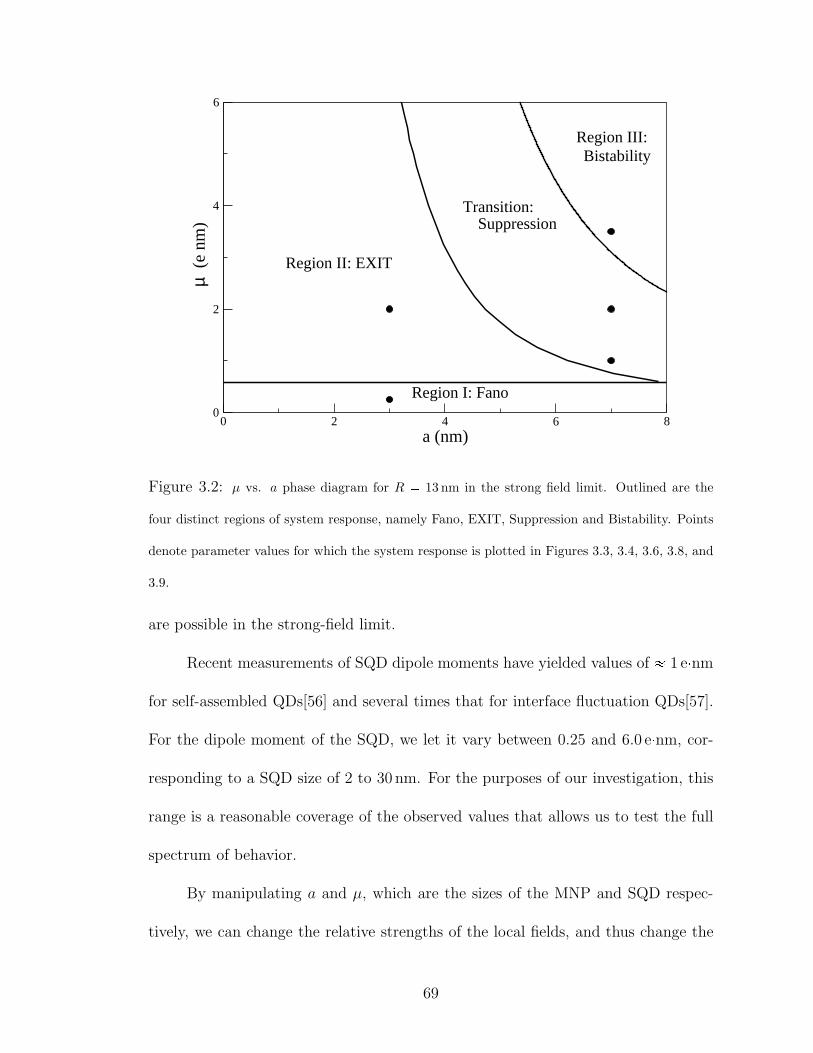
0 2 4 6 8a (nm)
0
2
4
6
µ (
e nm
)
Region II: EXIT
Region I: Fano
Region III:
Suppression
Bistability
Transition:
Figure 3.2: µ vs. a phase diagram for R 13 nm in the strong field limit. Outlined are the
four distinct regions of system response, namely Fano, EXIT, Suppression and Bistability. Points
denote parameter values for which the system response is plotted in Figures 3.3, 3.4, 3.6, 3.8, and
3.9.
are possible in the strong-field limit.
Recent measurements of SQD dipole moments have yielded values of 1 enmfor self-assembled QDs[56] and several times that for interface fluctuation QDs[57].
For the dipole moment of the SQD, we let it vary between 0.25 and 6.0 enm, cor-
responding to a SQD size of 2 to 30 nm. For the purposes of our investigation, this
range is a reasonable coverage of the observed values that allows us to test the full
spectrum of behavior.
By manipulating a and µ, which are the sizes of the MNP and SQD respec-
tively, we can change the relative strengths of the local fields, and thus change the
69
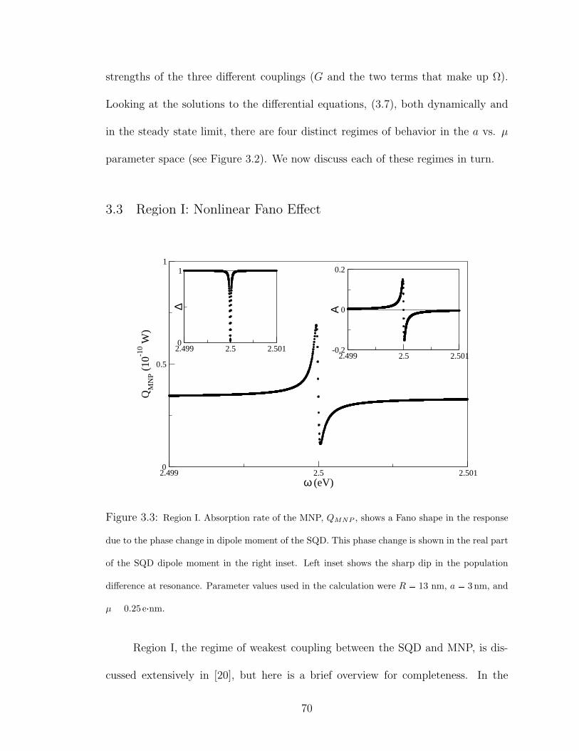
strengths of the three different couplings (G and the two terms that make up Ω).
Looking at the solutions to the differential equations, (3.7), both dynamically and
in the steady state limit, there are four distinct regimes of behavior in the a vs. µ
parameter space (see Figure 3.2). We now discuss each of these regimes in turn.
3.3 Region I: Nonlinear Fano Effect
2.499 2.5 2.5010
1
∆
2.499 2.5 2.501ω (eV)
0
0.5
1
QM
NP (
10-1
0 W)
2.499 2.5 2.501-0.2
0
0.2
A
Figure 3.3: Region I. Absorption rate of the MNP, QMNP , shows a Fano shape in the response
due to the phase change in dipole moment of the SQD. This phase change is shown in the real part
of the SQD dipole moment in the right inset. Left inset shows the sharp dip in the population
difference at resonance. Parameter values used in the calculation were R 13 nm, a 3 nm, and
µ 0.25 enm.
Region I, the regime of weakest coupling between the SQD and MNP, is dis-
cussed extensively in [20], but here is a brief overview for completeness. In the
70
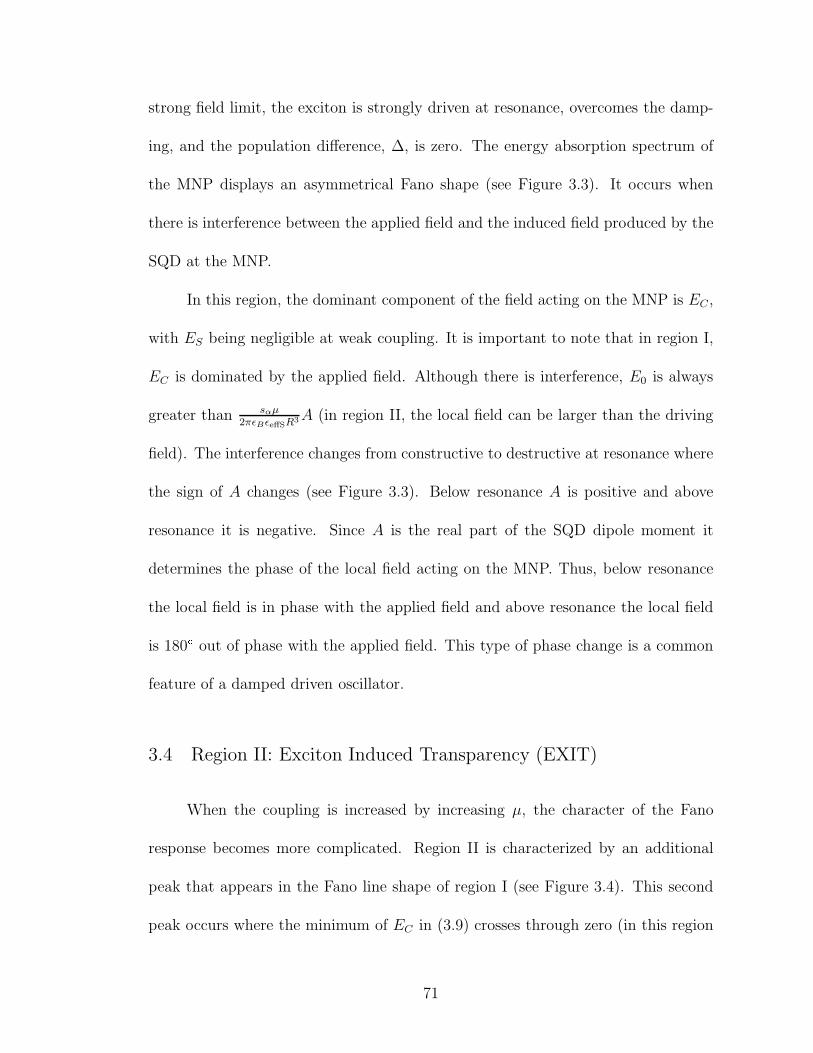
strong field limit, the exciton is strongly driven at resonance, overcomes the damp-
ing, and the population difference, ∆, is zero. The energy absorption spectrum of
the MNP displays an asymmetrical Fano shape (see Figure 3.3). It occurs when
there is interference between the applied field and the induced field produced by the
SQD at the MNP.
In this region, the dominant component of the field acting on the MNP is EC ,
with ES being negligible at weak coupling. It is important to note that in region I,
EC is dominated by the applied field. Although there is interference, E0 is always
greater than sαµ
2πǫBǫeffSR3A (in region II, the local field can be larger than the driving
field). The interference changes from constructive to destructive at resonance where
the sign of A changes (see Figure 3.3). Below resonance A is positive and above
resonance it is negative. Since A is the real part of the SQD dipole moment it
determines the phase of the local field acting on the MNP. Thus, below resonance
the local field is in phase with the applied field and above resonance the local field
is 180 out of phase with the applied field. This type of phase change is a common
feature of a damped driven oscillator.
3.4 Region II: Exciton Induced Transparency (EXIT)
When the coupling is increased by increasing µ, the character of the Fano
response becomes more complicated. Region II is characterized by an additional
peak that appears in the Fano line shape of region I (see Figure 3.4). This second
peak occurs where the minimum of EC in (3.9) crosses through zero (in this region
71
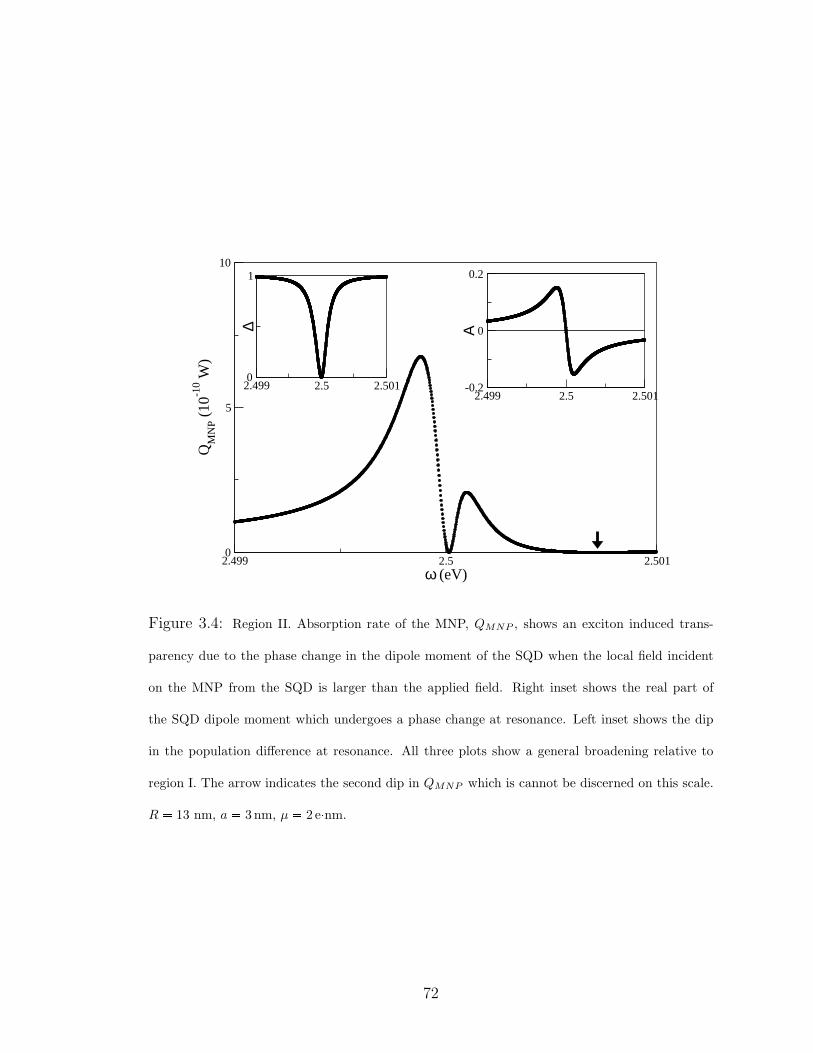
2.499 2.5 2.5010
1
∆
2.499 2.5 2.501ω (eV)
0
5
10
QM
NP (
10-1
0 W)
2.499 2.5 2.501-0.2
0
0.2
A
Figure 3.4: Region II. Absorption rate of the MNP, QMNP , shows an exciton induced trans-
parency due to the phase change in the dipole moment of the SQD when the local field incident
on the MNP from the SQD is larger than the applied field. Right inset shows the real part of
the SQD dipole moment which undergoes a phase change at resonance. Left inset shows the dip
in the population difference at resonance. All three plots show a general broadening relative to
region I. The arrow indicates the second dip in QMNP which is cannot be discerned on this scale.
R 13 nm, a 3 nm, µ 2 enm.
72

of parameter space, ES is still an order of magnitude smaller) (see Figure 3.5). For
this sign change to occur, the magnitude of the local field, sαµ
2πǫBǫeffSR3A, must be
larger than the applied field, E0, over a range of frequencies and must be out-of-
phase with E0 over these frequencies. As a consequence, EC changes sign just above
resonance (the dip in Figure 3.4). EC changes sign again, well above resonance (the
barely visible second dip in Figure 3.4), when the induced local field again becomes
weaker than the applied field. When EC changes sign at these two locations, the
field on the MNP is nearly completely canceled and the metal becomes reflective.
The absorption remains finite only because the small out-of-phase component ES
is non-zero. Because this is an interference effect between the driving field and the
field produced by the SQD, this is an exciton induced transparency (EXIT) in the
MNP that is due to the phase change at resonance of the driven SQD oscillator.
By setting EC 0, we find the line separating region I from region II to be
µpaq 2πǫ0ǫeffSR3E0
sαA. (3.10)
A varies with a slowly over the parameter space and thus µpaq is approximately
constant as a function of a. At the frequency where this double peak occurs, A has
a typical value of 0.15. Using this value for A, we can estimate this line to be
approximately µ 0.59 e nm.
When this line is found by numerically solving the differential equations re-
peatedly for different values of a and µ in this region, this line is determined to
be µpaq 0.574 e nm plus a small exponential term (negligible for a 10 nm).
This agrees extremely well with the value calculated by analyzing the behavior of
73
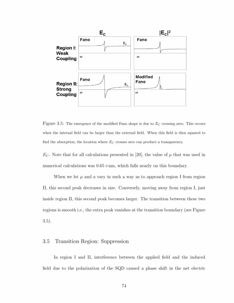
Figure 3.5: The emergence of the modified Fano shape is due to EC crossing zero. This occurs
when the internal field can be larger than the external field. When this field is then squared to
find the absorption, the location where EC crosses zero can produce a transparency.
EC . Note that for all calculations presented in [20], the value of µ that was used in
numerical calculations was 0.65 e nm, which falls nearly on this boundary.
When we let µ and a vary in such a way as to approach region I from region
II, this second peak decreases in size. Conversely, moving away from region I, just
inside region II, this second peak becomes larger. The transition between these two
regions is smooth i.e., the extra peak vanishes at the transition boundary (see Figure
3.5).
3.5 Transition Region: Suppression
In region I and II, interference between the applied field and the induced
field due to the polarization of the SQD caused a phase shift in the net electric
74
field incident on the MNP at resonance and an asymmetry in the response of the
MNP. However, this asymmetry is not manifested in the response of the SQD, i.e.
∆, (see Figure 3.4 for example) because the SQD does not couple directly to the
field produced by the polarization of the SQD. However, this field does couple to
the MNP, which in turn polarizes and produces a field that couples to the SQD.
This self-interaction of the SQD is G in Eq. (3.5). If the self-interaction becomes
significant, there will also be non-negligible interference of the electric fields at the
SQD. The interference then can suppress or enhance the response of the SQD.
2.499 2.5 2.5010
1
∆
2.499 2.5 2.501ω (eV)
0
20
40
QM
NP (
10-1
0 W)
2.499 2.5 2.501-0.2
0
0.2A
Figure 3.6: Transition region: weak suppression. Here we see the beginning of the suppression in
the response of the SQD, apparent in a slight asymmetry in ∆. Γb 98 µeV, Γa 37 µeV, with
suppression factor S 2.65. The double peaked EXIT structure is still visible, but the second
peak is much smaller relative to the main peak. The system response is also much broader than
in region I or II. Parameter values R 13 nm, a 7 nm, and µ 1 enm.
75
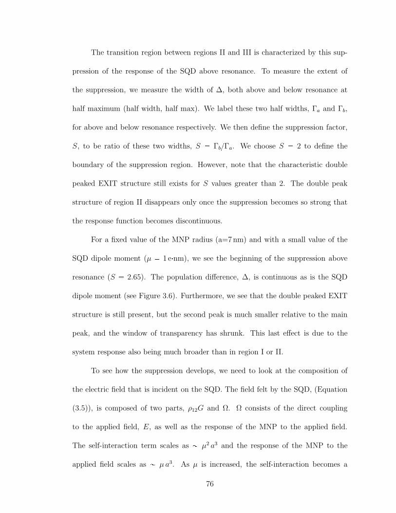
The transition region between regions II and III is characterized by this sup-
pression of the response of the SQD above resonance. To measure the extent of
the suppression, we measure the width of ∆, both above and below resonance at
half maximum (half width, half max). We label these two half widths, Γa and Γb,
for above and below resonance respectively. We then define the suppression factor,
S, to be ratio of these two widths, S ΓbΓa. We choose S 2 to define the
boundary of the suppression region. However, note that the characteristic double
peaked EXIT structure still exists for S values greater than 2. The double peak
structure of region II disappears only once the suppression becomes so strong that
the response function becomes discontinuous.
For a fixed value of the MNP radius (a=7 nm) and with a small value of the
SQD dipole moment (µ 1 enm), we see the beginning of the suppression above
resonance (S 2.65). The population difference, ∆, is continuous as is the SQD
dipole moment (see Figure 3.6). Furthermore, we see that the double peaked EXIT
structure is still present, but the second peak is much smaller relative to the main
peak, and the window of transparency has shrunk. This last effect is due to the
system response also being much broader than in region I or II.
To see how the suppression develops, we need to look at the composition of
the electric field that is incident on the SQD. The field felt by the SQD, (Equation
(3.5)), is composed of two parts, ρ12G and Ω. Ω consists of the direct coupling
to the applied field, E, as well as the response of the MNP to the applied field.
The self-interaction term scales as µ2 a3 and the response of the MNP to the
applied field scales as µ a3. As µ is increased, the self-interaction becomes a
76
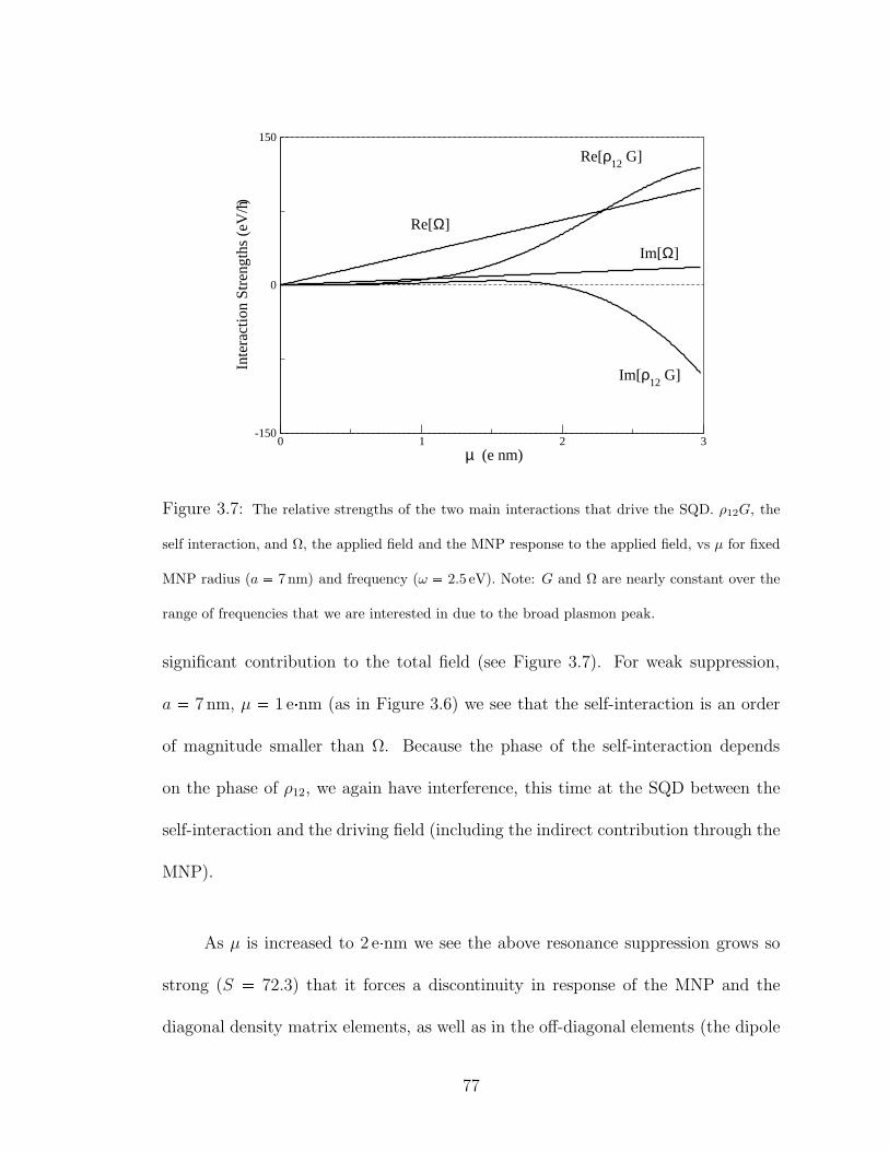
0 1 2 3 µ (e nm)
-150
0
150
Inte
ract
ion
Stre
ngth
s (e
V/h_ )
Re[Ω]
Re[ρ12
G]
Im[Ω]
Im[ρ12
G]
Figure 3.7: The relative strengths of the two main interactions that drive the SQD. ρ12G, the
self interaction, and Ω, the applied field and the MNP response to the applied field, vs µ for fixed
MNP radius (a 7 nm) and frequency (ω 2.5 eV). Note: G and Ω are nearly constant over the
range of frequencies that we are interested in due to the broad plasmon peak.
significant contribution to the total field (see Figure 3.7). For weak suppression,
a 7 nm, µ 1 enm (as in Figure 3.6) we see that the self-interaction is an order
of magnitude smaller than Ω. Because the phase of the self-interaction depends
on the phase of ρ12, we again have interference, this time at the SQD between the
self-interaction and the driving field (including the indirect contribution through the
MNP).
As µ is increased to 2 enm we see the above resonance suppression grows so
strong (S 72.3) that it forces a discontinuity in response of the MNP and the
diagonal density matrix elements, as well as in the off-diagonal elements (the dipole
77
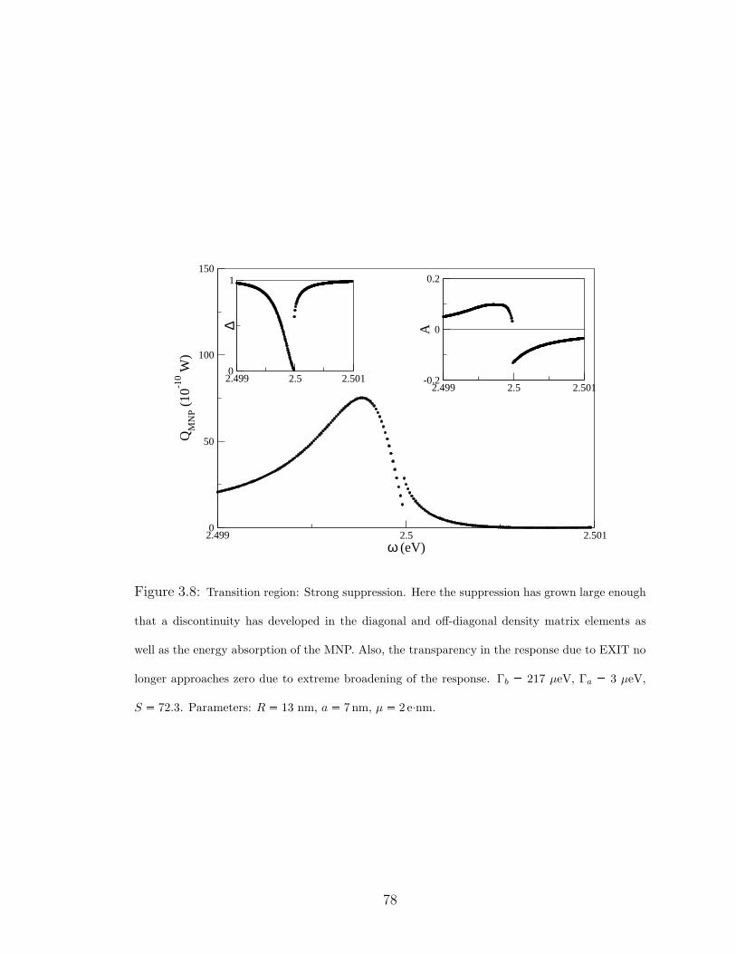
2.499 2.5 2.5010
1
∆
2.499 2.5 2.501ω (eV)
0
50
100
150
QM
NP (
10-1
0 W)
2.499 2.5 2.501-0.2
0
0.2
A
Figure 3.8: Transition region: Strong suppression. Here the suppression has grown large enough
that a discontinuity has developed in the diagonal and off-diagonal density matrix elements as
well as the energy absorption of the MNP. Also, the transparency in the response due to EXIT no
longer approaches zero due to extreme broadening of the response. Γb 217 µeV, Γa 3 µeV,
S 72.3. Parameters: R 13 nm, a 7 nm, µ 2 enm.
78
moment of the SQD) (see Figure 3.8). In this regime of strong suppression, we see
that the self-interaction is of the same order of magnitude as Ω (see Figure 3.7).
As µ is further increased, the suppression increases along with the discontinu-
ity, and the resonance of the SQD begins to shift to lower energies. The location
of phase change in ρ12 also splits based on the initial conditions of the system (see
Figure 3.13 and section 3.7.1), much like we will see in region III (which is discussed
in section 3.6). Further increase in µ results in further shifts to the resonance of the
SQD. This causes the suppression to eventually disappear. The discontinuity how-
ever, remains locked in for certain initial conditions, causing the bistability we will
see in the next section. As we will see there, at a large value of the dipole moment,
µ 3.5 enm, which is just inside region III, S is reduced to 1.7 (see Figure 3.9).
3.6 Region III: Bistability
When the coupling is further increased by increasing both µ and a, a region of
bistable response emerges (region III). In this limit, the field that is produced by the
SQD and then reflected off the MNP and back onto the SQD (the self-interaction
of the SQD) is sufficiently strong to introduce nonlinear effects into the response.
This, combined with an increased broadening due to the increased field strength,
causes the double peaked EXIT structure to disappear (see Figure 3.9).
Most importantly, region III is characterized by bistability in the steady state
solutions. For the same values µ and a, different initial conditions of ρ lead to
different steady states (compare Figures 3.9 and 3.10). This bistability only exists
79
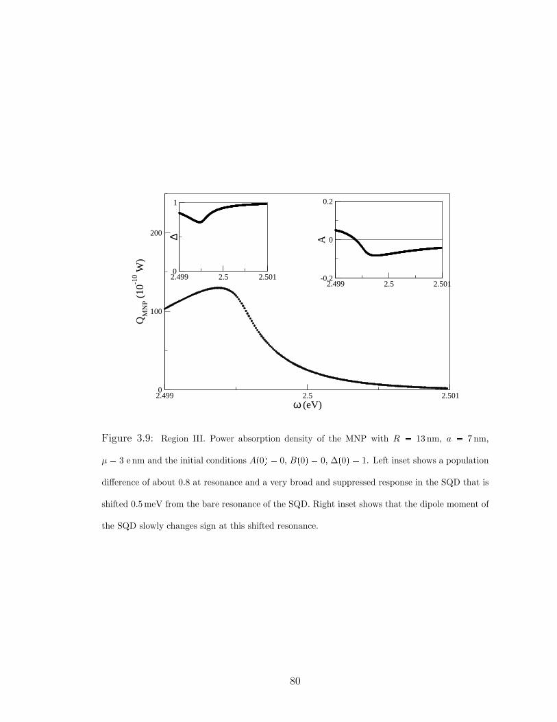
2.499 2.5 2.5010
1
∆
2.499 2.5 2.501ω (eV)
0
100
200
QM
NP (
10-1
0 W)
2.499 2.5 2.501-0.2
0
0.2
A
Figure 3.9: Region III. Power absorption density of the MNP with R 13 nm, a 7 nm,
µ 3 e nm and the initial conditions Ap0q 0, Bp0q 0, ∆p0q 1. Left inset shows a population
difference of about 0.8 at resonance and a very broad and suppressed response in the SQD that is
shifted 0.5meV from the bare resonance of the SQD. Right inset shows that the dipole moment of
the SQD slowly changes sign at this shifted resonance.
80
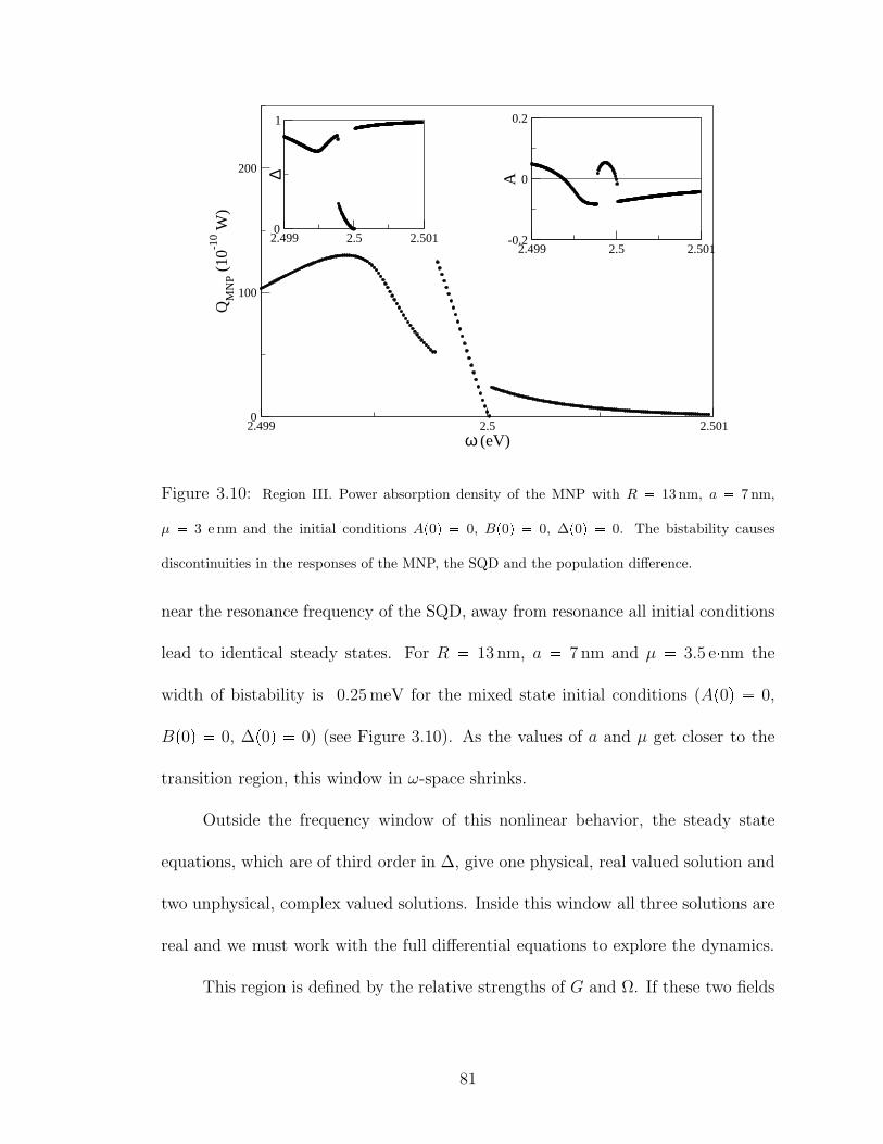
2.499 2.5 2.5010
1
∆
2.499 2.5 2.501ω (eV)
0
100
200
QM
NP (
10-1
0 W)
2.499 2.5 2.501-0.2
0
0.2
AFigure 3.10: Region III. Power absorption density of the MNP with R 13 nm, a 7 nm,
µ 3 e nm and the initial conditions Ap0q 0, Bp0q 0, ∆p0q 0. The bistability causes
discontinuities in the responses of the MNP, the SQD and the population difference.
near the resonance frequency of the SQD, away from resonance all initial conditions
lead to identical steady states. For R 13 nm, a 7 nm and µ 3.5 enm the
width of bistability is 0.25meV for the mixed state initial conditions (Ap0q 0,
Bp0q 0, ∆p0q 0) (see Figure 3.10). As the values of a and µ get closer to the
transition region, this window in ω-space shrinks.
Outside the frequency window of this nonlinear behavior, the steady state
equations, which are of third order in ∆, give one physical, real valued solution and
two unphysical, complex valued solutions. Inside this window all three solutions are
real and we must work with the full differential equations to explore the dynamics.
This region is defined by the relative strengths of G and Ω. If these two fields
81
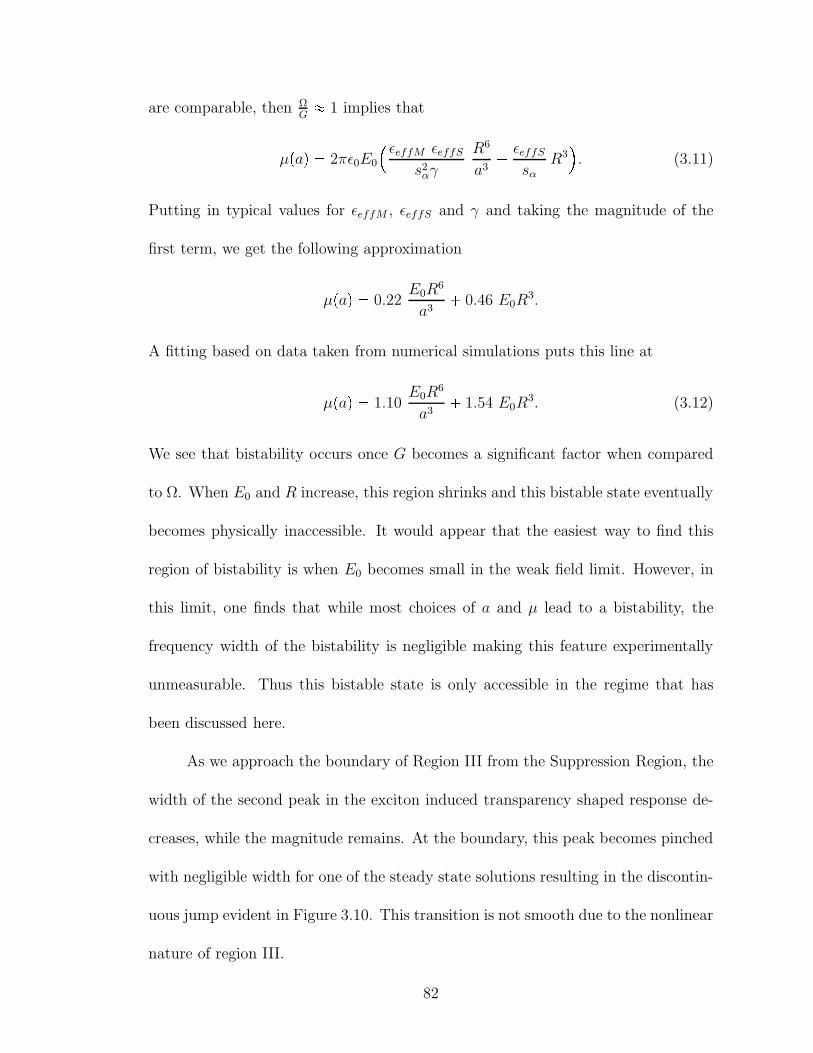
are comparable, then ΩG 1 implies that
µpaq 2πǫ0E0
ǫeffM ǫeffS
s2αγ
R6
a3 ǫeffS
sαR3. (3.11)
Putting in typical values for ǫeffM , ǫeffS and γ and taking the magnitude of the
first term, we get the following approximation
µpaq 0.22E0R
6
a3 0.46 E0R
3.
A fitting based on data taken from numerical simulations puts this line at
µpaq 1.10E0R
6
a3 1.54 E0R
3. (3.12)
We see that bistability occurs once G becomes a significant factor when compared
to Ω. When E0 and R increase, this region shrinks and this bistable state eventually
becomes physically inaccessible. It would appear that the easiest way to find this
region of bistability is when E0 becomes small in the weak field limit. However, in
this limit, one finds that while most choices of a and µ lead to a bistability, the
frequency width of the bistability is negligible making this feature experimentally
unmeasurable. Thus this bistable state is only accessible in the regime that has
been discussed here.
As we approach the boundary of Region III from the Suppression Region, the
width of the second peak in the exciton induced transparency shaped response de-
creases, while the magnitude remains. At the boundary, this peak becomes pinched
with negligible width for one of the steady state solutions resulting in the discontin-
uous jump evident in Figure 3.10. This transition is not smooth due to the nonlinear
nature of region III.
82
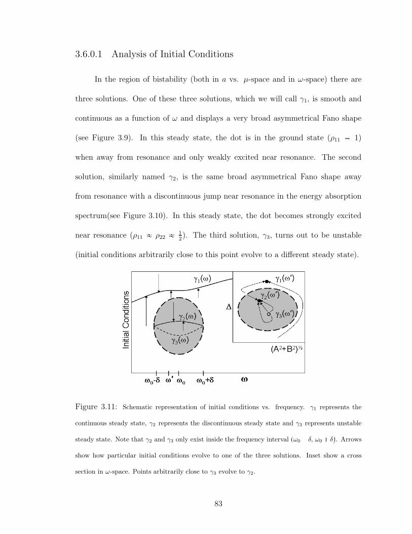
3.6.0.1 Analysis of Initial Conditions
In the region of bistability (both in a vs. µ-space and in ω-space) there are
three solutions. One of these three solutions, which we will call γ1, is smooth and
continuous as a function of ω and displays a very broad asymmetrical Fano shape
(see Figure 3.9). In this steady state, the dot is in the ground state (ρ11 1)
when away from resonance and only weakly excited near resonance. The second
solution, similarly named γ2, is the same broad asymmetrical Fano shape away
from resonance with a discontinuous jump near resonance in the energy absorption
spectrum(see Figure 3.10). In this steady state, the dot becomes strongly excited
near resonance (ρ11 ρ22 12). The third solution, γ3, turns out to be unstable
(initial conditions arbitrarily close to this point evolve to a different steady state).
Figure 3.11: Schematic representation of initial conditions vs. frequency. γ1 represents the
continuous steady state, γ2 represents the discontinuous steady state and γ3 represents unstable
steady state. Note that γ2 and γ3 only exist inside the frequency interval pω0 δ, ω0 δq. Arrowsshow how particular initial conditions evolve to one of the three solutions. Inset show a cross
section in ω-space. Points arbitrarily close to γ3 evolve to γ2.
83
The space of initial conditions can be divided into 2 regions, one for each of the
two possible, stable, steady-state solutions. For a particular choice of parameters
(R 13 nm, a 7 nm, µ 3.5 e nm) the region with the discontinuous solution
is an ellipsoid centered at Ap0q 0, Bp0q 0, ∆p0q 0 and is found through
numerical calculations to be approximately given by the relation
4Ap0q2 Bp0q2∆p0q2 ¤ 0.07 (3.13)
with the region outside this ellipsoid having the smooth solution. The unstable
solution is a line through this space parameterized by ω in the interval pω0δ, ωδq.It can begin inside or outside of the region given by (3.13), but near resonance is
always inside for cases we looked at (see Figure 3.11). For initial conditions exactly
on this line, the state remains unchanged as it evolves in time. All other initial
states evolve to γ1 or γ2.
As the initial conditions get close to the boundary of this region, the width
(δω 2δ) shrinks. Numerically, the relationship between the initial conditions and
this width was found to be approximately4Ap0q2 Bp0q2∆p0q22 δω
4 103eV
2 0.005 .
3.6.1 Calculation of the Resonance Shift
We saw in section 3.5 that as the coupling between the SQD and the MNP
is increased and the transition is made into region III, there is a redshift in the
resonance of the SQD. Accompanied with this redshift, there was a broadening of
the response and a small population of the exciton excited state, i.e. ∆ at resonance
84
is no longer nearly zero (see Figure 3.9 for an example of both of these effects).
We can model both the redshift and the new minimum of ∆. Starting with
(3.7), we set the left hand side to zero to arrive at the steady state equations. Taking
the first two equations and solving for A and B in terms of ∆ we have
A ∆kΩI δωΩR
k2 δω2
B ∆kΩR δωΩI
k2 δω2
∆ 1 τ0
4ΩIA 4ΩRB 4GIpA2 B2q (3.14)
where we have defined
k ∆GI 1
T0
δω ω ω0 ∆GR .
We now take the derivative with respect to ω for each of the equations in
(3.14). To find the minimum of ∆, we evaluate them at the critical point ω ωc
and set ∆1pωcq 0.
A1 ∆2δωkΩI pk2 δω2qΩRpk2 δω2q2
(3.15)
B1 ∆2δωkΩR pk2 δω2qΩIpk2 δω2q2
(3.16)
∆1 τ0
4ΩIA
1 4ΩRB1 8GIpAA1 BB1q 0 (3.17)
Note that G and Ω are nearly constant over the range of frequencies that we consider
because the plasmon peak is broad in comparison, thus we take their derivatives with
respect to ω to be zero. Putting (3.15) and (3.16) into (3.17), and after a bit of
algebra, we arrive at the result
0 ∆c δω ,
85
where ∆c ∆pωcq. ∆c cannot take a value of zero in the steady state, except in
the limit that τ0 Ñ 8 (this is easy to check), so we must have δω 0. Using this
result, we find that at ω ωc we have A ∆cΩI
kand B ∆c
ΩR
k. Then,
∆c 1 4τ0pΩ2
R Ω2Iq
GI
∆cGI
k ∆2
cG2I
k2
.
Note, that the only assumption we have made thus far is that the steady state
exists. To proceed further, we now look at the region of parameter space where
the resonance frequency shifts relative to the natural frequency ω0. Since we are
interested in the case in which a shift is seen in the resonance frequency (recalling
that this coincides with ∆ no longer being nearly zero), we take ∆c to have a value
greater than 0.01 and we have that 1T0∆cGI 1. Thus, we can expand k1 and
k2. In this case, we have
∆c 1 4τ0pΩ2
R Ω2Iq
T0G2I∆c
.
Solving this quadratic equation for ∆c and expanding the square root of the dis-
criminant we have
∆c 1 4τ0pΩ2
R Ω2Iq
T0G2I
... (3.18)
So, our resonance occurs at
ωc ω0 GR
1 4
τ0pΩ2R Ω2
IqT0G
2I
. (3.19)
Using these approximations for ∆c and ωc, for typical parameters µ 4 enmand a 7 nm, our approximations give ∆c 0.84 and ωc ω0 0.82 meV.
Solving the differential equations numerically we find these two quantities to be
86
∆c 0.81 and ωc ω0 0.79 meV, respectively, in excellent agreement with our
approximations.
Looking at our expressions that describe the redshift and the minimum of ∆,
we see that the turning on of these effects is controlled by the ratio pΩ2R Ω2
IqG2I .
As we’ll see in the next section, this ratio will largely determine the strength of the
coupling to the imaginary component of the SQD dipole moment, B, with respect
to the coupling to A. This increase in the coupling to the imaginary part of the
SQD dipole moment (which has a damping effect on the system) causes the redshift
in the SQD resonance and the decrease in the exciton population at resonance. In
the next section, we’ll see that this also causes the suppression to turn off.
3.7 Running (the) Interference: Phasors and Interaction Strengths
To better understand these interference effects, it is helpful to view the fields
as phasors in the complex plane (see Figure 3.12). First consider a case of weak
coupling (small µ). For weak coupling, Ω is much larger than G and we can ignore
the effect of G (as was shown in Figure 3.7). Thus our resultant field on the SQD
is mostly in the direction of Ω which is along the real axis both above and below
resonance (see Figure 3.12). This has the effect of driving the SQD mostly by the
real field, i.e. the SQD couples more strongly to A than to B.
However, when the coupling is increased so that G is no longer negligible,
the field the SQD sees from the self coupling is ρ12G. Below resonance, ρ12G is
in phase with the applied field, but above resonance, it is out of phase with the
87
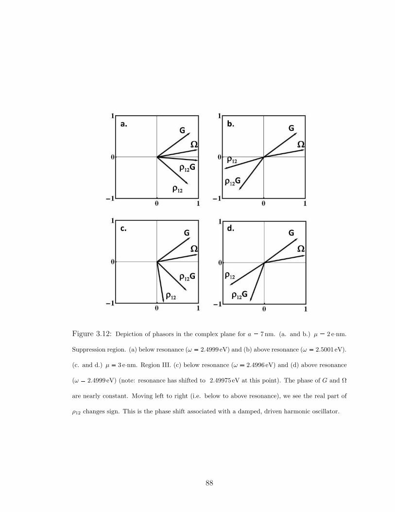
Figure 3.12: Depiction of phasors in the complex plane for a 7 nm. (a. and b.) µ 2 enm.
Suppression region. (a) below resonance (ω 2.4999 eV) and (b) above resonance (ω 2.5001eV).
(c. and d.) µ 3 enm. Region III. (c) below resonance (ω 2.4996 eV) and (d) above resonance
(ω 2.4999eV) (note: resonance has shifted to 2.49975eV at this point). The phase of G and Ω
are nearly constant. Moving left to right (i.e. below to above resonance), we see the real part of
ρ12 changes sign. This is the phase shift associated with a damped, driven harmonic oscillator.
88
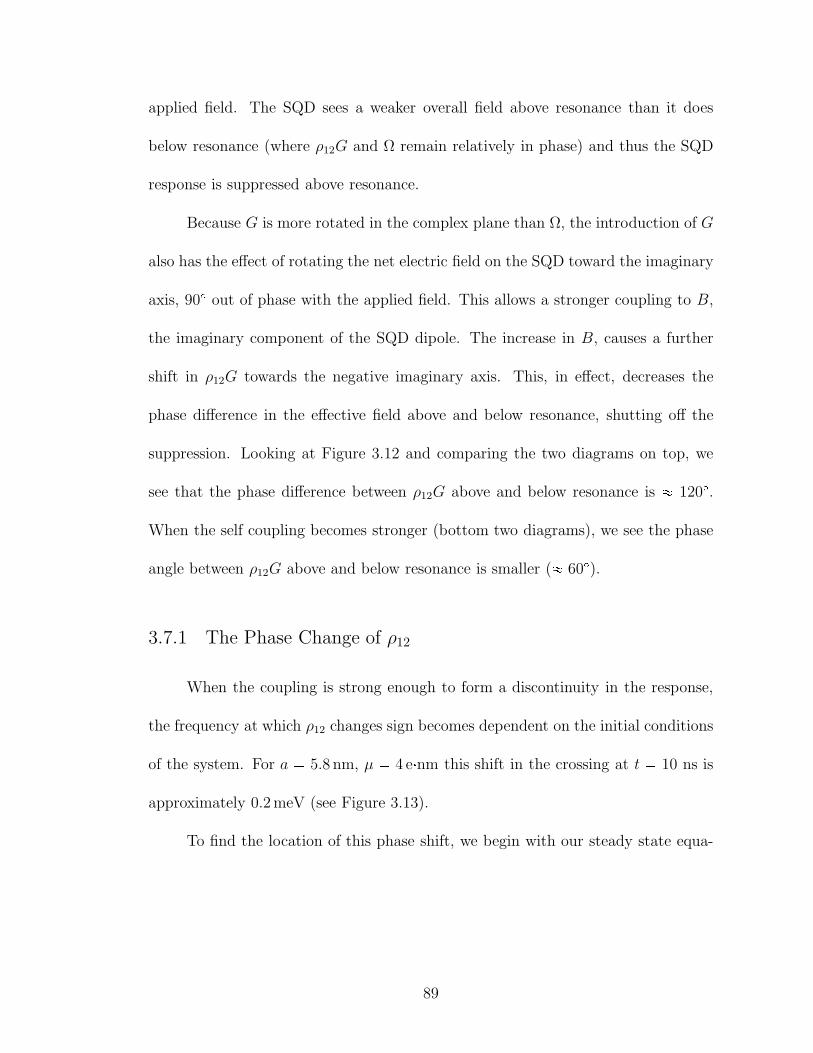
applied field. The SQD sees a weaker overall field above resonance than it does
below resonance (where ρ12G and Ω remain relatively in phase) and thus the SQD
response is suppressed above resonance.
Because G is more rotated in the complex plane than Ω, the introduction of G
also has the effect of rotating the net electric field on the SQD toward the imaginary
axis, 90 out of phase with the applied field. This allows a stronger coupling to B,
the imaginary component of the SQD dipole. The increase in B, causes a further
shift in ρ12G towards the negative imaginary axis. This, in effect, decreases the
phase difference in the effective field above and below resonance, shutting off the
suppression. Looking at Figure 3.12 and comparing the two diagrams on top, we
see that the phase difference between ρ12G above and below resonance is 120.When the self coupling becomes stronger (bottom two diagrams), we see the phase
angle between ρ12G above and below resonance is smaller ( 60).3.7.1 The Phase Change of ρ12
When the coupling is strong enough to form a discontinuity in the response,
the frequency at which ρ12 changes sign becomes dependent on the initial conditions
of the system. For a 5.8 nm, µ 4 enm this shift in the crossing at t 10 ns is
approximately 0.2meV (see Figure 3.13).
To find the location of this phase shift, we begin with our steady state equa-
89
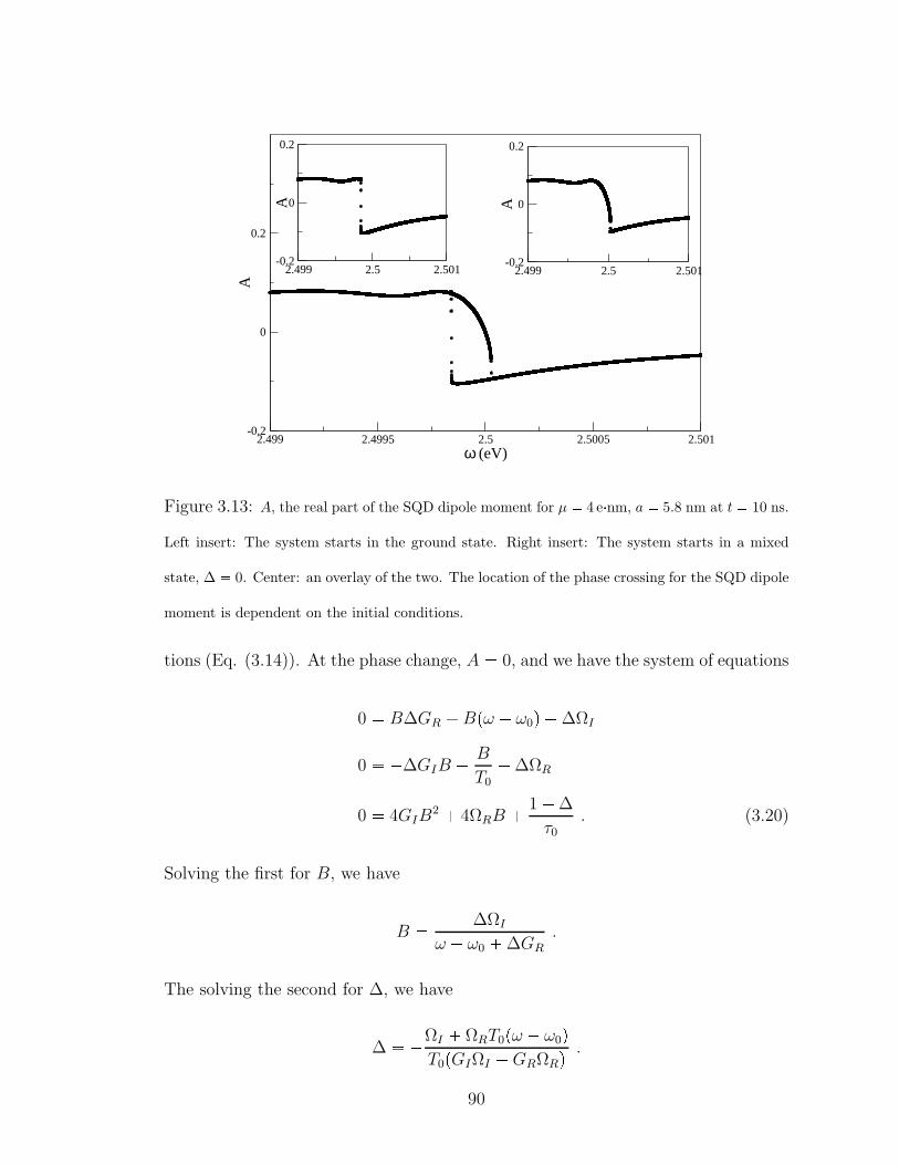
2.499 2.5 2.501-0.2
0
0.2
A
2.499 2.4995 2.5 2.5005 2.501ω (eV)
-0.2
0
0.2A
2.499 2.5 2.501-0.2
0
0.2
AFigure 3.13: A, the real part of the SQD dipole moment for µ 4 enm, a 5.8 nm at t 10 ns.
Left insert: The system starts in the ground state. Right insert: The system starts in a mixed
state, ∆ 0. Center: an overlay of the two. The location of the phase crossing for the SQD dipole
moment is dependent on the initial conditions.
tions (Eq. (3.14)). At the phase change, A 0, and we have the system of equations
0 B∆GR Bpω ω0q ∆ΩI
0 ∆GIB B
T0∆ΩR
0 4GIB2 4ΩRB 1∆
τ0. (3.20)
Solving the first for B, we have
B ∆ΩI
ω ω0 ∆GR
.
The solving the second for ∆, we have
∆ ΩI ΩRT0pω ω0qT0pGIΩI GRΩRq .
90
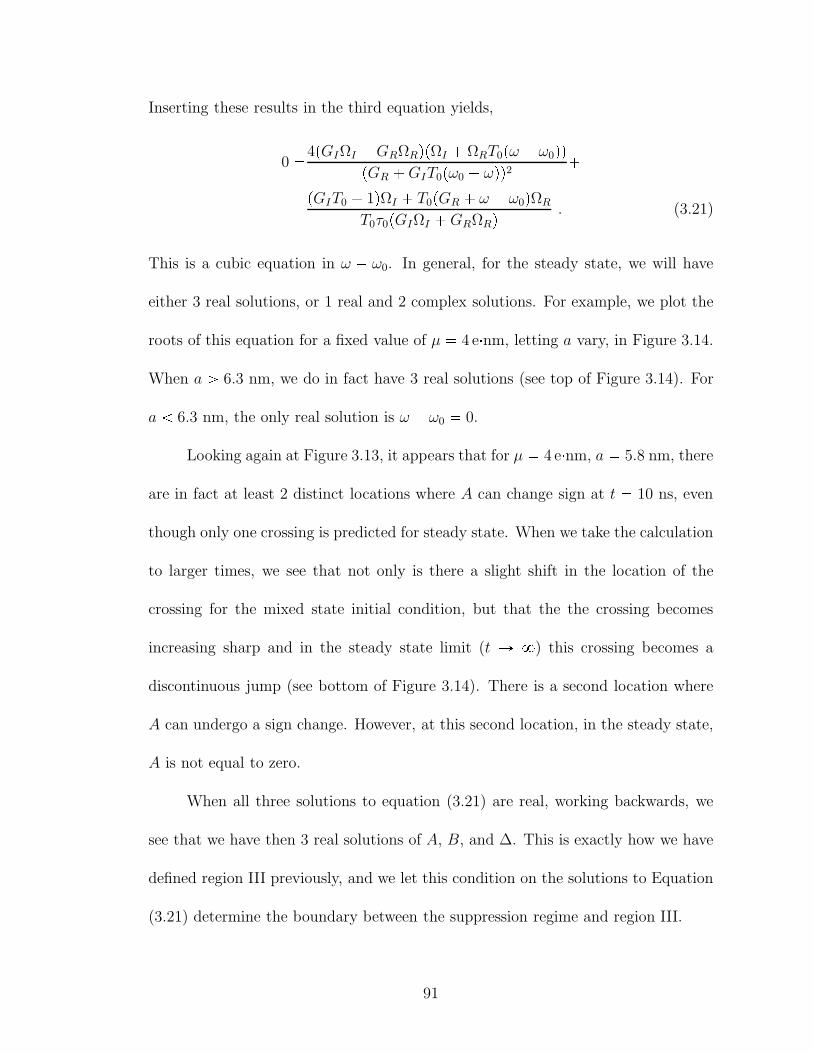
Inserting these results in the third equation yields,
0 4pGIΩI GRΩRqpΩI ΩRT0pω ω0qqpGR GIT0pω0 ωqq2 pGIT0 1qΩI T0pGR ω ω0qΩR
T0τ0pGIΩI GRΩRq . (3.21)
This is a cubic equation in ω ω0. In general, for the steady state, we will have
either 3 real solutions, or 1 real and 2 complex solutions. For example, we plot the
roots of this equation for a fixed value of µ 4 enm, letting a vary, in Figure 3.14.
When a ¡ 6.3 nm, we do in fact have 3 real solutions (see top of Figure 3.14). For
a 6.3 nm, the only real solution is ω ω0 0.
Looking again at Figure 3.13, it appears that for µ 4 enm, a 5.8 nm, there
are in fact at least 2 distinct locations where A can change sign at t 10 ns, even
though only one crossing is predicted for steady state. When we take the calculation
to larger times, we see that not only is there a slight shift in the location of the
crossing for the mixed state initial condition, but that the the crossing becomes
increasing sharp and in the steady state limit (t Ñ 8) this crossing becomes a
discontinuous jump (see bottom of Figure 3.14). There is a second location where
A can undergo a sign change. However, at this second location, in the steady state,
A is not equal to zero.
When all three solutions to equation (3.21) are real, working backwards, we
see that we have then 3 real solutions of A, B, and ∆. This is exactly how we have
defined region III previously, and we let this condition on the solutions to Equation
(3.21) determine the boundary between the suppression regime and region III.
91
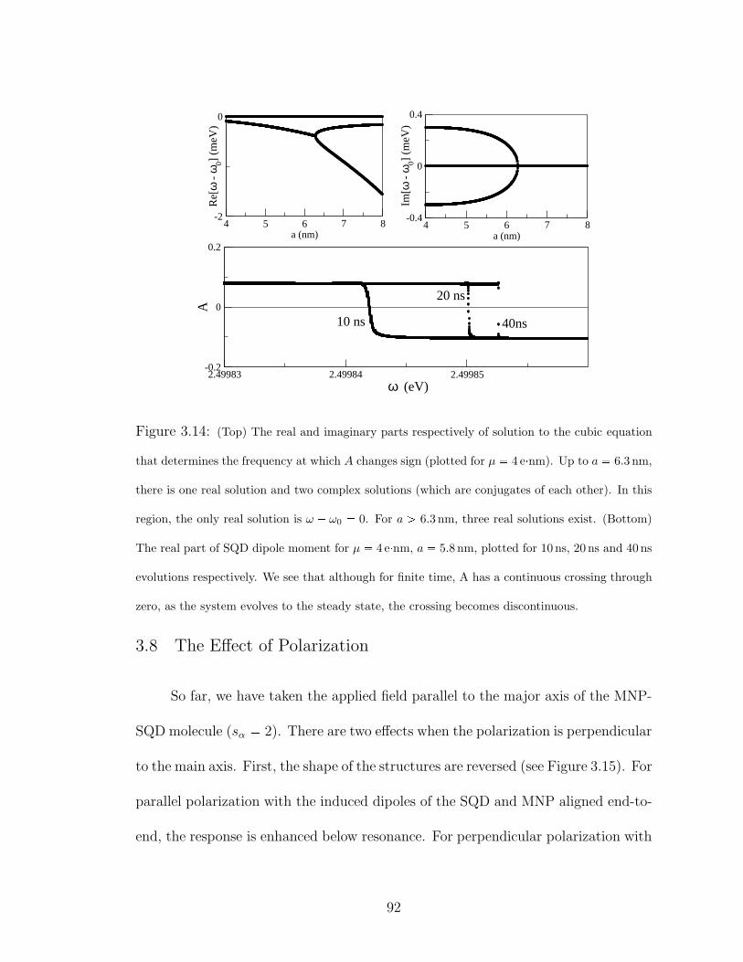
2.49983 2.49984 2.49985 ω (eV)
-0.2
0
0.2
A
4 5 6 7 8a (nm)
-0.4
0
0.4
Im[ω
- ω
0] (m
eV)
4 5 6 7 8a (nm)
-2
0
Re[
ω -
ω0]
(meV
)
20 ns
10 ns 40ns
Figure 3.14: (Top) The real and imaginary parts respectively of solution to the cubic equation
that determines the frequency at which A changes sign (plotted for µ 4 enm). Up to a 6.3 nm,
there is one real solution and two complex solutions (which are conjugates of each other). In this
region, the only real solution is ω ω0 0. For a ¡ 6.3 nm, three real solutions exist. (Bottom)
The real part of SQD dipole moment for µ 4 enm, a 5.8 nm, plotted for 10 ns, 20 ns and 40 ns
evolutions respectively. We see that although for finite time, A has a continuous crossing through
zero, as the system evolves to the steady state, the crossing becomes discontinuous.
3.8 The Effect of Polarization
So far, we have taken the applied field parallel to the major axis of the MNP-
SQD molecule (sα 2). There are two effects when the polarization is perpendicular
to the main axis. First, the shape of the structures are reversed (see Figure 3.15). For
parallel polarization with the induced dipoles of the SQD and MNP aligned end-to-
end, the response is enhanced below resonance. For perpendicular polarization with
92
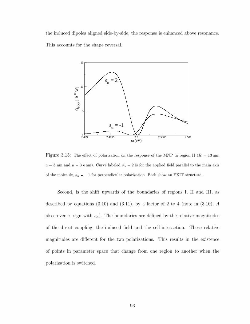
the induced dipoles aligned side-by-side, the response is enhanced above resonance.
This accounts for the shape reversal.
2.499 2.4995 2.5 2.5005 2.501ω (eV)
0
5
10
15
QM
NP (
10-1
0 W)
sα = 2
sα = -1
Figure 3.15: The effect of polarization on the response of the MNP in region II (R 13 nm,
a 3 nm and µ 3 e nm). Curve labeled sα 2 is for the applied field parallel to the main axis
of the molecule, sα 1 for perpendicular polarization. Both show an EXIT structure.
Second, is the shift upwards of the boundaries of regions I, II and III, as
described by equations (3.10) and (3.11), by a factor of 2 to 4 (note in (3.10), A
also reverses sign with sα). The boundaries are defined by the relative magnitudes
of the direct coupling, the induced field and the self-interaction. These relative
magnitudes are different for the two polarizations. This results in the existence
of points in parameter space that change from one region to another when the
polarization is switched.
93
3.9 A Summary of Findings
To summarize, in this chapter we have investigated the optical response of a
semiconductor quantum dot coupled with a metal nanoparticle. We have probed
the strong applied electric field limit, where local induced fields are comparable
to the driving field. We treated the SQD quantum mechanically in the density
matrix formalism and the MNP as a classical spherical dielectric. We saw that the
behavior of this system is highly dependent on the relative sizes of the MNP and SQD
and by varying, µ and a, we found four distinct regimes of behavior in the strong
field limit which each exhibit novel properties. By numerically probing parameter
space we were able to set bounds on each of these regions. Furthermore, we were
able to connect these numerical approximations of these boundaries to relationships
amongst the various coupling strengths which allowed for a deeper understanding
of how these behaviors emerge.
In the region of weak coupling, region I, we found that the energy absorption
spectrum displays an asymmetrical Fano shape as previously predicted. It occurs
when there is interference between the applied field and the internal field produced
by the SQD at the location of the MNP. In the strong coupling regime, we saw that
the behavior was more complex. As the SQD is increased in size (thus the coupling
is increased), the asymmetrical Fano effect of region I is modified by the appearance
of an additional peak with a deep minimum between the peaks. Here, the induced
local field at the MNP becomes larger than the applied field, for frequencies near
the SQD resonance. As such, the interference of the field from the SQD with the
94
applied electric field now results in a sign change in the net electric field at the
MNP above resonance where the two fields are out-of-phase. An exciton induced
transparency (EXIT) arises in the MNP response when there is nearly complete
destructive interference between these two fields acting on the MNP.
A further increase in coupling strength moves the system into a transition
regime, where the EXIT structure is modified with a discontinuous jump in response
of the system (in both the diagonal and off-diagonal density matrix elements) and
the response of the SQD is highly suppressed above resonance in this transition.
This suppression comes about because the response of the SQD is that of a driven,
damped harmonic oscillator. Specifically, this behavior is seen in the response of
SQD dipole moment. As in the case of the classical damped driven oscillator, the
behavior of the system is determined by the whether the driving frequency is above
or below the resonance frequency of the system. Below resonance the dipole moment
of the SQD is in phase with the driving field, and above resonance it is 180 out
of phase. Since the phase of the self interaction of the SQD is determined by the
phase of its own dipole moment, there is destructive interference above resonance
and constructive interference below resonance, between the applied field and the
self interaction field. EXIT is determined by the interference between the fields that
drive the MNP. Suppression is determined by the interference among the fields that
drive the SQD. In both cases, the phase of some of the fields changes at resonance,
leading to a crossover from constructive to destructive interference. The fields that
do change phase at resonance originate from the phase change in the SQD dipole
moment that occurs at resonance.
95
As the coupling is further increased by increasing the sizes of both the SQD
and MNP, the self-interaction of the SQD becomes significant in region III. Here,
we found an extreme broadening of the response that washes out the second peak
of the EXIT. More interestingly, we found that the response is nonlinear. This
nonlinearity is due to the significant self interaction of the SQD (feedback through
the MNP). In this regime, we found the existence of multiple steady state solutions
leading to a bistability where one of the two stable solutions has a discontinuous
energy spectrum. Furthermore, we saw that coupling to the imaginary part of the
SQD dipole moment largely determines whether EXIT, suppression or bistability in
the system is visible.
We have predicted phenomena that could emerge from an SQD-MNP hybrid
molecule, and just as importantly, we have located in parameter space where these
phenomena occur, and what causes them to emerge. How the various system fields
interfere, constructively and destructively, is central in determining system response.
This understanding is critical if one is to know how to generalize these results to
similar system and more complicated structures. In the next chapter we will see
how this knowledge could be exploited in order to engineer MNP-SQD systems that
are tailored towards a desired system behavior. In particular, we will show how to
engineer hybrid systems that will best display this behavior.
96
Chapter 4
Engineered SQD-MNP Systems with Extended Geometries
So far we have studied the interactions between an SQD and a spherical MNP,
using the dipole approximation for the field emitted from the MNP. The geometry
of these hybrid systems determines the nature of the local fields and couplings,
which in turn determines the system behavior. Useful devices that will utilize these
structures will require more complicated geometries than what we have previously
explored. To consider more complex MNP structures, for example, nanorods and
nanowires, chains of MNPs, and SQDs at various positions in the structure, a more
complete calculational method for the local fields needs to be employed than was
used in the previous chapter (i.e. using a non-retarded, dipole approximation for
the MNP response). In this chapter we will utilize the boundary element method
(BEM) to fully account for the response electric fields of such complex structures.
4.1 Introduction
There are two basic interactions that the SQD participates in. One is the
coupling due to an applied plane wave driving field (both directly with the driving
field and from the response of the MNP to the applied plane wave). The second
is the self-interaction of the SQD in which the MNP responds to the polarization
field of the SQD and in turn produces a field felt back at the SQD. As we saw in
97
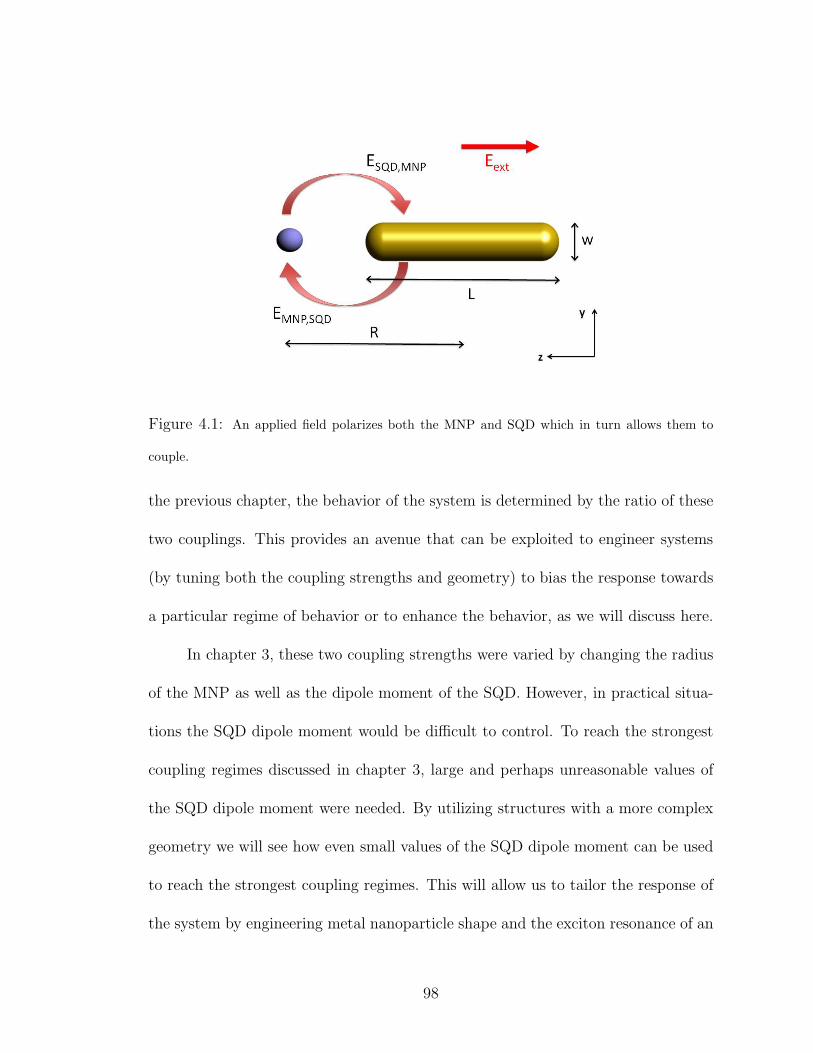
Figure 4.1: An applied field polarizes both the MNP and SQD which in turn allows them to
couple.
the previous chapter, the behavior of the system is determined by the ratio of these
two couplings. This provides an avenue that can be exploited to engineer systems
(by tuning both the coupling strengths and geometry) to bias the response towards
a particular regime of behavior or to enhance the behavior, as we will discuss here.
In chapter 3, these two coupling strengths were varied by changing the radius
of the MNP as well as the dipole moment of the SQD. However, in practical situa-
tions the SQD dipole moment would be difficult to control. To reach the strongest
coupling regimes discussed in chapter 3, large and perhaps unreasonable values of
the SQD dipole moment were needed. By utilizing structures with a more complex
geometry we will see how even small values of the SQD dipole moment can be used
to reach the strongest coupling regimes. This will allow us to tailor the response of
the system by engineering metal nanoparticle shape and the exciton resonance of an
98
SQD in order to control the individual local near-fields that couple the MNP and
the SQD.
The effect of MNP size, shape and SQD placement will be analyzed to deter-
mine the regimes where the local multipolar response becomes significant. We will
identify regimes where dark modes and higher order multipolar modes can influence
the hybrid response. External fields do not directly drive MNP dark modes, so
SQD/MNP coupling is dominated by the local induced coupling, providing a situ-
ation in which the induced self-interaction could be probed using near field tech-
niques. All of these aspects could enhance the capabilities of metal nanostructures
to provide spatial and spectral control of the optical properties of single emitters.
In section 2 we discuss the hybrid molecule in detail, allowing for a more
complex structure. The MNP is taken as a classical dielectric with a response
calculated with the BEM. Upon finding the resultant fields acting on the SQD, we
use a density matrix approach to treat the SQD. Once the behavior of the SQD
is found, we then use that information to calculate the local near fields of our
hybrid molecule. We also calculate the energy absorption of the MNP and provide
details on how numerical calculations were carried out. In section 3 we discuss the
conditions when a full electrodynamical calculation should be used for a spherical
MNP rather than a multipole expansion or dipole approximation. We also apply the
BEM to study the response of a nanorod. In section 4 we discuss how coupling the
SQD to a nanorod allows the system to be engineered toward a particular regime of
behavior. Here we exploit coupling to the dark states of the nanorod to investigate
the self-interaction of the SQD. We present our conclusions in section 5.
99
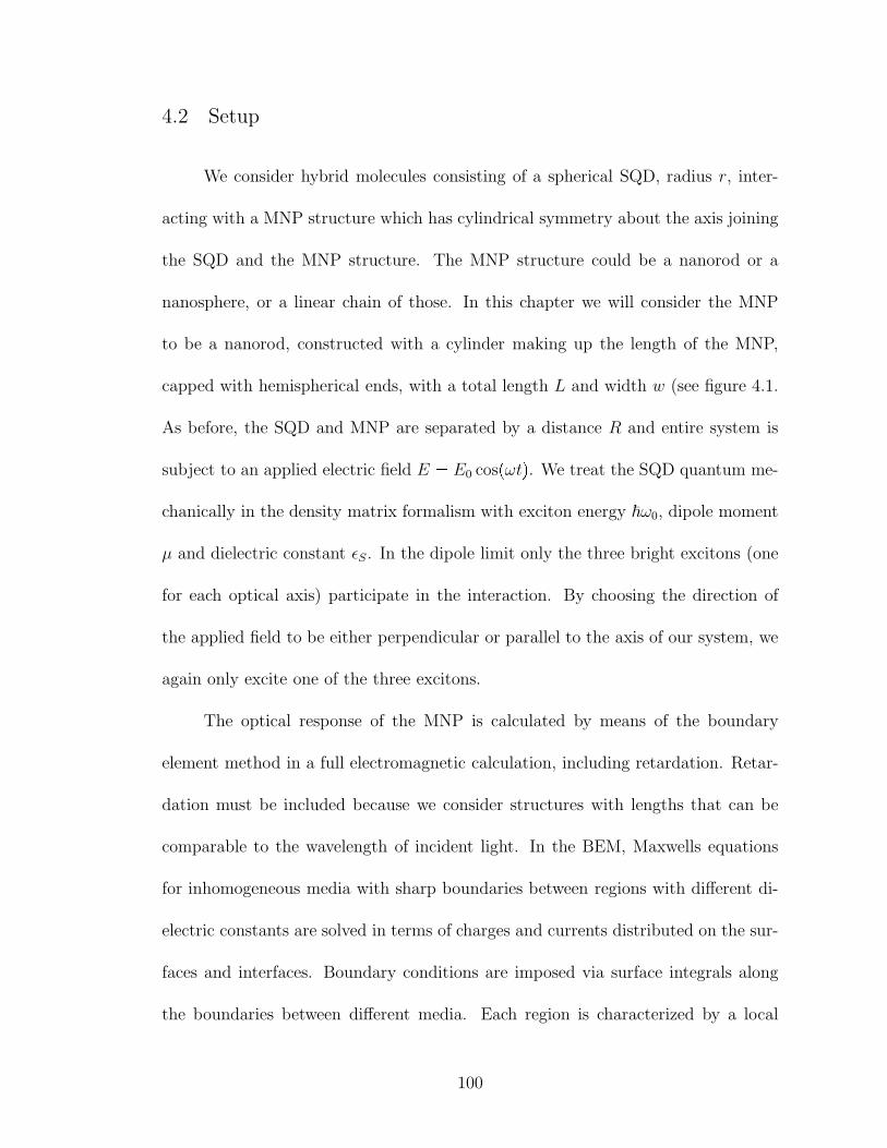
4.2 Setup
We consider hybrid molecules consisting of a spherical SQD, radius r, inter-
acting with a MNP structure which has cylindrical symmetry about the axis joining
the SQD and the MNP structure. The MNP structure could be a nanorod or a
nanosphere, or a linear chain of those. In this chapter we will consider the MNP
to be a nanorod, constructed with a cylinder making up the length of the MNP,
capped with hemispherical ends, with a total length L and width w (see figure 4.1.
As before, the SQD and MNP are separated by a distance R and entire system is
subject to an applied electric field E E0 cospωtq. We treat the SQD quantum me-
chanically in the density matrix formalism with exciton energy ~ω0, dipole moment
µ and dielectric constant ǫS. In the dipole limit only the three bright excitons (one
for each optical axis) participate in the interaction. By choosing the direction of
the applied field to be either perpendicular or parallel to the axis of our system, we
again only excite one of the three excitons.
The optical response of the MNP is calculated by means of the boundary
element method in a full electromagnetic calculation, including retardation. Retar-
dation must be included because we consider structures with lengths that can be
comparable to the wavelength of incident light. In the BEM, Maxwells equations
for inhomogeneous media with sharp boundaries between regions with different di-
electric constants are solved in terms of charges and currents distributed on the sur-
faces and interfaces. Boundary conditions are imposed via surface integrals along
the boundaries between different media. Each region is characterized by a local
100
dielectric function. The external fields interact self-consistently with the induced
boundary charges and currents, which are determined by discretizing the surface
integrals and solving the appropriate matrix equations. In this approach, the scat-
tered field due to an incident external field is calculated directly. We calculate, in
this way, both the near and far fields for a given MNP from both a plane wave
source as well as from a dipole source (the SQD). In handling the dipole source, we
take a quasi-static approach and do not include the time dependence of the dipole
moment in Maxwell’s equations.
As before, our Hamiltonian for the two level SQD, HSQD, is
HSQD ~ω0a:a µESQD pa a:q , (4.1)
where a and a: are the exciton annihilation and creation operators. ESQD is the
total electric field felt by the SQD and consists of the applied, external field, E, and
the induced, internal field, produced by the polarization of the MNP. The MNP is
polarized by the applied plane wave and we denote the response field as Eplanewave.
The MNP is also polarized by the dipole field produced by the SQD and this response
field we denote Edipole. Taking into account screening, we can then write ESQD as
ESQD 1
ǫeffS
E Eplanewave Edipole
, (4.2)
where ǫeffS 2ǫBǫS3ǫB
. ǫB is a background dielectric constant which would correspond
to the medium in which the system is embedded. Writing the applied field as
E E0cospωtq E0
2eiωt E0
2eiωt and the response from the MNP due to a unit
plane wave with positive frequency as Ep (which will be calculated using BEM),
101
then
Eplanewave E0
2Ep e
iωt E0
2E
p eiωt.
We make use of the density matrix ρ to calculate the polarization of the SQD.
We label the ground state of our SQD (no exciton) as level 1 and the excited state
(one exciton) we label as level 2. We then have for the polarization, PSQD µpρ12 ρ21q (see [48]). Factoring out the high frequency time dependence of the
off-diagonal terms of the density matrix, we define
ρ12 rρ12 eiωtρ21 rρ21 eiωt . (4.3)
We write the response of the MNP due to a dipole source with positive fre-
quency at the location of the SQD as Ed (again calculated with BEM and evaluated
at the location of the SQD). Taking into account the screening at the dipole, we
then have,
Edipole µ
ǫeffSrρ21Ed e
iωt µ
ǫeffSrρ12E
d eiωt.
Putting these expressions for Eplanewave and Edipole into equation (4.2), as well as
writing out the applied field explicitly, we have
ESQD 1
ǫeffS
E0
2p1 Epq µ
ǫeffSrρ21Ed
eiωt h.c., (4.4)
In order to write this in a more familiar form, we make the following definitions
G µ2
~ǫ2effSEd
Ω µE0
2~ǫeffSp1 Epq,
102
in terms of the responses, Ep and Ed, to a unit plane wave and unit dipole, respec-
tively. Once we know Ep and Ed, the theory proceeds as it did in chapter 3. Again
we can identify G as the self-interaction of the SQD, the first term in Ω as the direct
coupling to the applied field and the second term in Ω as arising from the MNP
response to the applied field. We again write the field acting on the SQD as,
ESQD ~
µ
"pΩG rρ21q eiωt pΩ G rρ12q eiωt*. (4.5)
We solve the master equation9ρ i
~rρ,HSQDs Γpρq , (4.6)
where Γpρq is the relaxation matrix with entries Γ11 ρ111
τ0, Γ12 Γ21 ρ12
T20and
Γ22 ρ22τ0. Again we separate real and imaginary parts, and write the density matrix
elements as rρ12 A iBrρ21 A iB
∆ ρ11 ρ22 .
To solve (4.6), we make the rotating wave approximation. When changing the
Hamiltonian to the interaction picture we keep terms that oscillate like eipωω0qtand neglect terms that oscillate like eipωω0qt. Making use of our definitions and the
rotating wave approximation, we have the same set of coupled differential equations,9A A
T20 pω ω0qB ΩI GIAGRB
∆9B B
T20 pω ω0qA ΩR GRAGIB
∆9∆ 1∆
τ0 4ΩIA 4ΩRB 4GIpA2 B2q, (4.7)
103
where GR, GI , ΩR and ΩI are the real and imaginary parts of G and Ω respectively.
We solve this set of differential equations as we did previously in chapter 3.
4.2.1 System Energy
As before, the rate at which energy is absorbed by our system consists of two
parts, QSQD and QMNP . The SQD absorbs energy by the creation of an exciton
followed by a non-radiative decay. The rate is just QSQD ~ω0ρ22τ0. To calculate
the energy absorbed by the MNP, we take the time average of the volume integral,³j E dv., where j is the local current density. To calculate the fields inside the MNP
we again employ the BEM. We denote the field inside the MNP due to the dipole
field of the SQD as Epinsideqdipole . This field includes the field due to the polarization
induced in the MNP as well as the dipole field of the SQD. Similarly, we denote
the field inside the MNP due to the applied plane wave as Epinsideqplanewave and this field
includes the field due to the polarization induced in the MNP as well as the applied
field. These fields with positive frequency can be determined once Eid (the field
inside the MNP due to a unit dipole with positive frequency at the SQD) and Eip
(the field inside the MNP due to a unit incident plane wave with positive frequency)
are known. We write
Epinsideqdipole µ
ǫeffSrρ21Ei
d eiωt µ
ǫeffSrρ12pEi
dq eiωtEpinsideqplanewave E0
2Ei
p eiωt E0
2pEi
pq eiωt ,in a notation similar to what we have previously employed. Thus the field inside
the MNP is just the sum of these two fields. We calculate the current density, j as
104
we did in chapter 3, j ǫmpωqBEBt and again take the time derivatives of rρ12 andrρ21 to be zero and we then have for the local current, j,
j iω
"ǫmpωqE0
2Ei
p µ
ǫeffSrρ21Ei
d
eiωt ǫmpωqE0
2pEi
pq µ
ǫeffSrρ12pEi
dqeiωt* .We can now calculate j E,
j E iω#ǫmpωqE0
2Ei
p µ
ǫeffSrρ21Ei
d
2
e2iωt ǫmpωqE0
2pEi
pq µ
ǫeffSrρ12pEi
dq2
e2iωt 2iImrǫmpωqsE0
2pEi
pq µ
ǫeffSrρ12 pEi
dq2+ .Taking the time average of this result over the period of fast oscillation and inte-
grating over the volume of the MNP yields QMNP ,
QMNP 2ωImrǫmpωqs » E0
2pEi
pq µ
ǫeffSrρ21pEi
dq2 dv.We calculate this integral numerically using the BEM to find pEi
pq and pEidq and
equation (4.7) to find rρ21 in the steady state limit.
4.2.2 Numerical Calculations in the Large Field Limit
In this paper we take our MNP to have cylindrical symmetry about the z-axis
and we take the dielectric constant of the background to be ǫB ǫ0. We model the
MNP as a cylinder with hemispherical ends, with total length L and total width w
(see Figure 4.1). Thus, in the case of L w, we have a sphere of radius w2. The
SQD is placed on the positive z-axis a distance R from the center of the MNP. We
105
consider the large field limit (intensity of 103W/cm2) and we take the polarization
of the applied electric field parallel to the axis of our SQD-MNP molecule (the z
direction) with the propagation along the x direction. We take ǫmpωq as the bulk
dielectric constant of gold as found experimentally [55]. For the SQD, we take
ǫS 6 ǫ0 and the exciton resonant frequency to be in the range of 1 4 eV. For the
relaxation times of the SQD we take τ0 0.8 ns and T20 0.3 ns.
4.3 Advantages of Using a Full Electrodynamical Description
Previously, calculations have been done on a system consisting of an SQD
interacting with a spherical MNP in the dipole limit[20, 21, 22] as well as in the
multipole limit[23], both of which are a non-retarded approach. In the dipole limit,
the ratio of MNP radius, a, to MNP-SQD separation, R, should be small (as the
multipole expansion is a power series in p aRq2). For a 7 nm, R 13 nm, the first
order correction is nearly 30%.
In [23] it was shown that for a 15 nm, R 20 nm, the sum of the first 10
terms of the multipole expansion of the coupling strength between the MNP and
SQD is almost 7 times greater than that given by only the first term in the series
(the dipole limit). The most interesting hybrid molecules are those with strong
coupling. One manner of increasing the coupling strength between the MNP and
SQD is to place the SQD very close to the MNP, thus, the correction due to higher
order multipole terms will be important in the systems we most wish to study.
106
4.3.1 Comparison Between a Full Electrodynamical Calculation and
a Non-Retarded Multipole Expansion for Spherical MNPs
In order to compare the results obtained using the BEM with those given
by the quasi-static multipole expansion, we compare the values of G given by the
two methods, because there is no multipolar correction to the response due to the
applied plane wave. In the multipole limit, G is given by the expression (see ref.
[23])
G 8n1
snγna2n1µ2
4πǫB ~ ǫ2effSR2n4
, (4.8)
where
γn ǫmpωq ǫB
ǫmpωq n1nǫB,
and sn pn 1q2 or P 1np1q for polarization parallel or perpendicular to the z-axis
and P 1n is the first derivative of the Legendre function. When we take only the term
with n 1, we recover the dipole approximation. In order to calculate the fields in
the multipole expansion for systems where the total separation is very nearly equal
to the radius of the MNP (R a), many terms are needed for convergence of (4.8).
For a spherical MNP with R 60 nm and a 40 nm, we see an enhancement
in the imaginary part ofG of nearly a factor of two. We also see a slight enhancement
of 25% and a red shift on the order of 0.1 eV in the peak of the real part of G
(see figure 4.2). When this calculation is carried out over a large subset of MNP
sizes and separation, this enhancement increases as the MNP radius is increased for
fixed separation up to a MNP radius of approximately 50 nm (except in the most
extreme cases of very small separation) or if the separation is increased for fixed
107
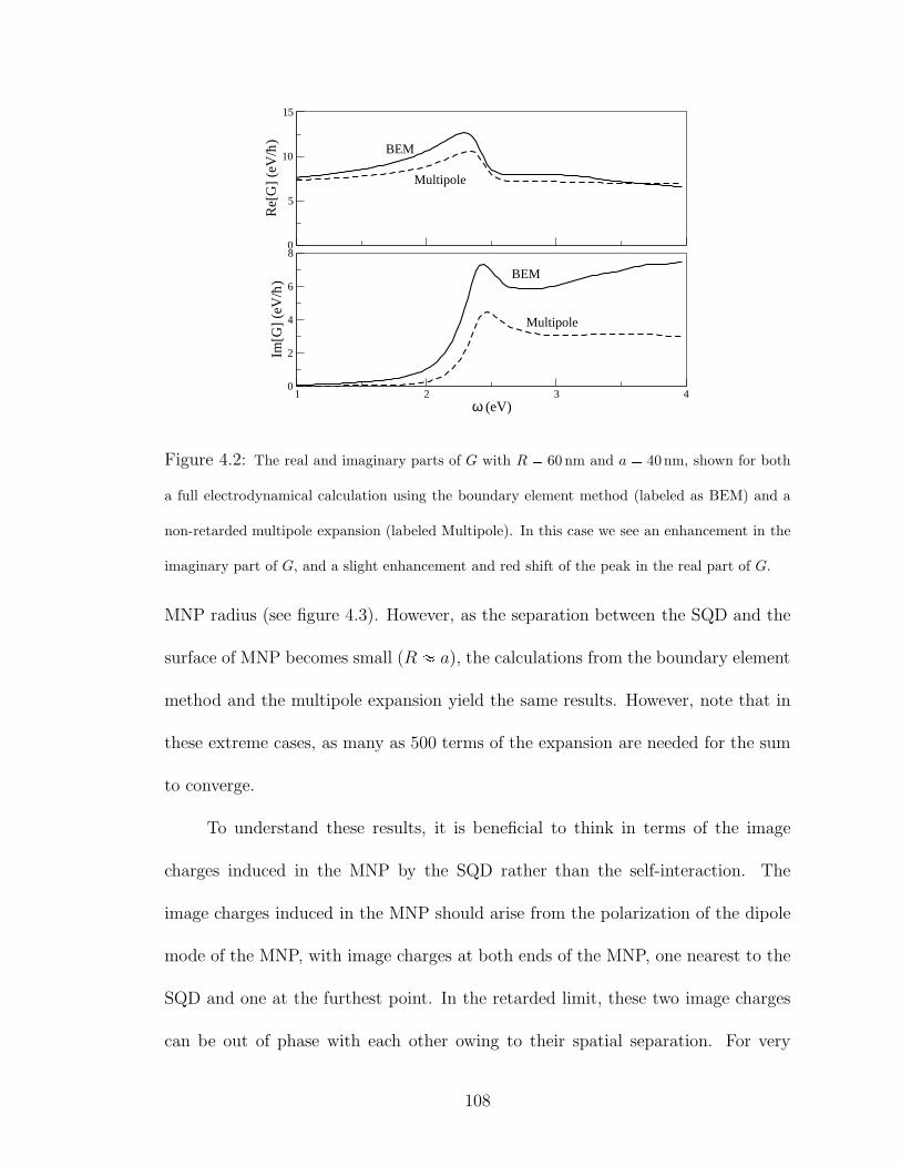
0
5
10
15
Re[
G]
(eV
/h_ )
1 2 3 4ω (eV)
0
2
4
6
8
Im[G
] (e
V/h_ )
BEM
BEM
Multipole
Multipole
Figure 4.2: The real and imaginary parts of G with R 60 nm and a 40nm, shown for both
a full electrodynamical calculation using the boundary element method (labeled as BEM) and a
non-retarded multipole expansion (labeled Multipole). In this case we see an enhancement in the
imaginary part of G, and a slight enhancement and red shift of the peak in the real part of G.
MNP radius (see figure 4.3). However, as the separation between the SQD and the
surface of MNP becomes small (R a), the calculations from the boundary element
method and the multipole expansion yield the same results. However, note that in
these extreme cases, as many as 500 terms of the expansion are needed for the sum
to converge.
To understand these results, it is beneficial to think in terms of the image
charges induced in the MNP by the SQD rather than the self-interaction. The
image charges induced in the MNP should arise from the polarization of the dipole
mode of the MNP, with image charges at both ends of the MNP, one nearest to the
SQD and one at the furthest point. In the retarded limit, these two image charges
can be out of phase with each other owing to their spatial separation. For very
108
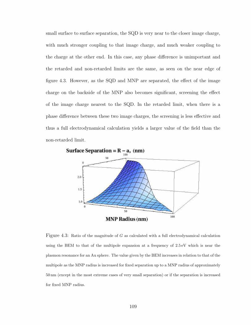
small surface to surface separation, the SQD is very near to the closer image charge,
with much stronger coupling to that image charge, and much weaker coupling to
the charge at the other end. In this case, any phase difference is unimportant and
the retarded and non-retarded limits are the same, as seen on the near edge of
figure 4.3. However, as the SQD and MNP are separated, the effect of the image
charge on the backside of the MNP also becomes significant, screening the effect
of the image charge nearest to the SQD. In the retarded limit, when there is a
phase difference between these two image charges, the screening is less effective and
thus a full electrodynamical calculation yields a larger value of the field than the
non-retarded limit.
Figure 4.3: Ratio of the magnitude of G as calculated with a full electrodynamical calculation
using the BEM to that of the multipole expansion at a frequency of 2.5 eV which is near the
plasmon resonance for an Au sphere. The value given by the BEM increases in relation to that of the
multipole as the MNP radius is increased for fixed separation up to a MNP radius of approximately
50 nm (except in the most extreme cases of very small separation) or if the separation is increased
for fixed MNP radius.
109
4.3.2 From Spheres to Rods
For most systems of interest involving a spherical MNP and a SQD (i.e. for
small separation), both the multipole method and the BEM will yield similar results.
The main advantage of using the BEM is that we can study any shape of MNP we
choose. Also, one can study the effects of placing the SQD off the symmetry axis.
Moreover, the multipole expansion only has a simple form in the cases that the
applied field is perpendicular or parallel to the molecular axis.
When we replace the spherical MNP with a nanorod the effect on coupling can
be quite dramatic (see Figure 4.4). Holding the width of the nanorod fixed at 14 nm,
as we move from a wire of length 14 nm (which is a 7 nm radius sphere) to a wire
of length 150 nm, we see an enhancement in the value of ΩR of approximately an
order of magnitude, and of ΩI of nearly 25 times at the peak value (see figure 4.4).
Whereas the peak values of G remain relatively unchanged, we do see higher order
modes appear in the spectrum. At L 150 nm a total of 3 peaks have appeared in
G (at 1.1, 1.7 and 2.1 eV) whereas there are only 2 in Ω (at 1.1 and 2.1 eV). We also
note a redshift in the principle plasmon peak for both G and Ω.
As we saw last chapter, the ratios of the various components of G and Ω are
key in determining the behavior of the SQD-MNP molecule. The more complicated
spectrum provided by a wire, yields a much broader range of system behavior. The
enhancement provided by a wire also allows for the regimes of strongest coupling to
be more easily accessed experimentally.
110
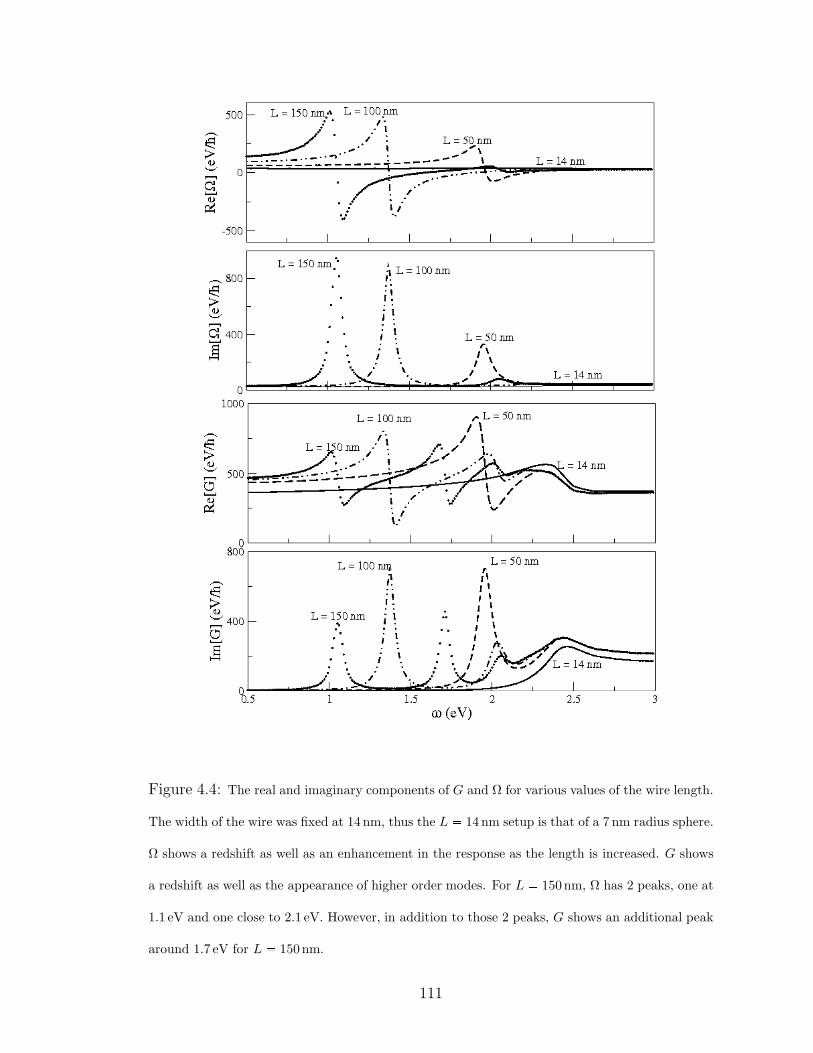
Figure 4.4: The real and imaginary components of G and Ω for various values of the wire length.
The width of the wire was fixed at 14 nm, thus the L 14 nm setup is that of a 7 nm radius sphere.
Ω shows a redshift as well as an enhancement in the response as the length is increased. G shows
a redshift as well as the appearance of higher order modes. For L 150nm, Ω has 2 peaks, one at
1.1 eV and one close to 2.1 eV. However, in addition to those 2 peaks, G shows an additional peak
around 1.7 eV for L 150nm.
111
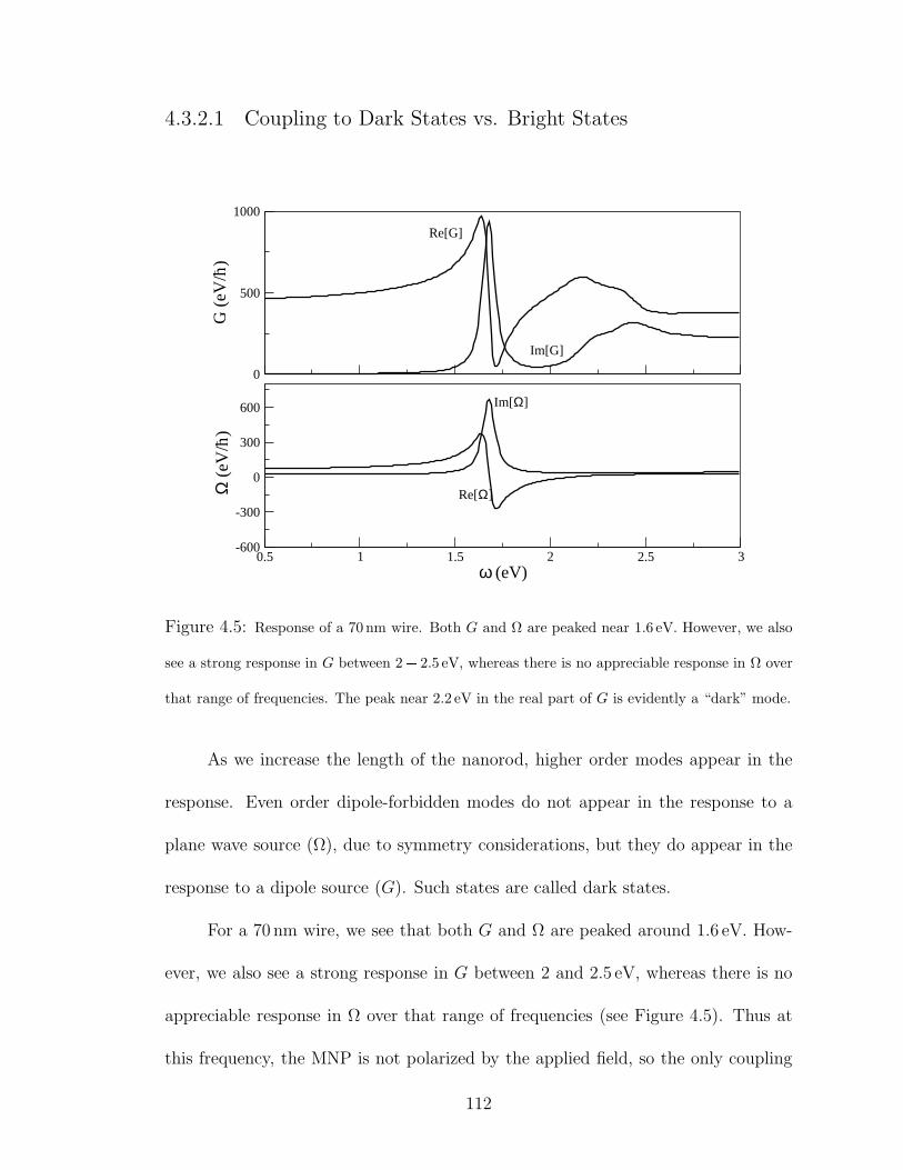
4.3.2.1 Coupling to Dark States vs. Bright States
0
500
1000G
(eV
/h_ )
0.5 1 1.5 2 2.5 3ω (eV)
-600
-300
0
300
600
Ω (
eV/h_ )
Re[G]
Im[G]
Re[Ω]
Im[Ω]
Figure 4.5: Response of a 70 nm wire. Both G and Ω are peaked near 1.6 eV. However, we also
see a strong response in G between 2 2.5 eV, whereas there is no appreciable response in Ω over
that range of frequencies. The peak near 2.2 eV in the real part of G is evidently a “dark” mode.
As we increase the length of the nanorod, higher order modes appear in the
response. Even order dipole-forbidden modes do not appear in the response to a
plane wave source (Ω), due to symmetry considerations, but they do appear in the
response to a dipole source (G). Such states are called dark states.
For a 70 nm wire, we see that both G and Ω are peaked around 1.6 eV. How-
ever, we also see a strong response in G between 2 and 2.5 eV, whereas there is no
appreciable response in Ω over that range of frequencies (see Figure 4.5). Thus at
this frequency, the MNP is not polarized by the applied field, so the only coupling
112
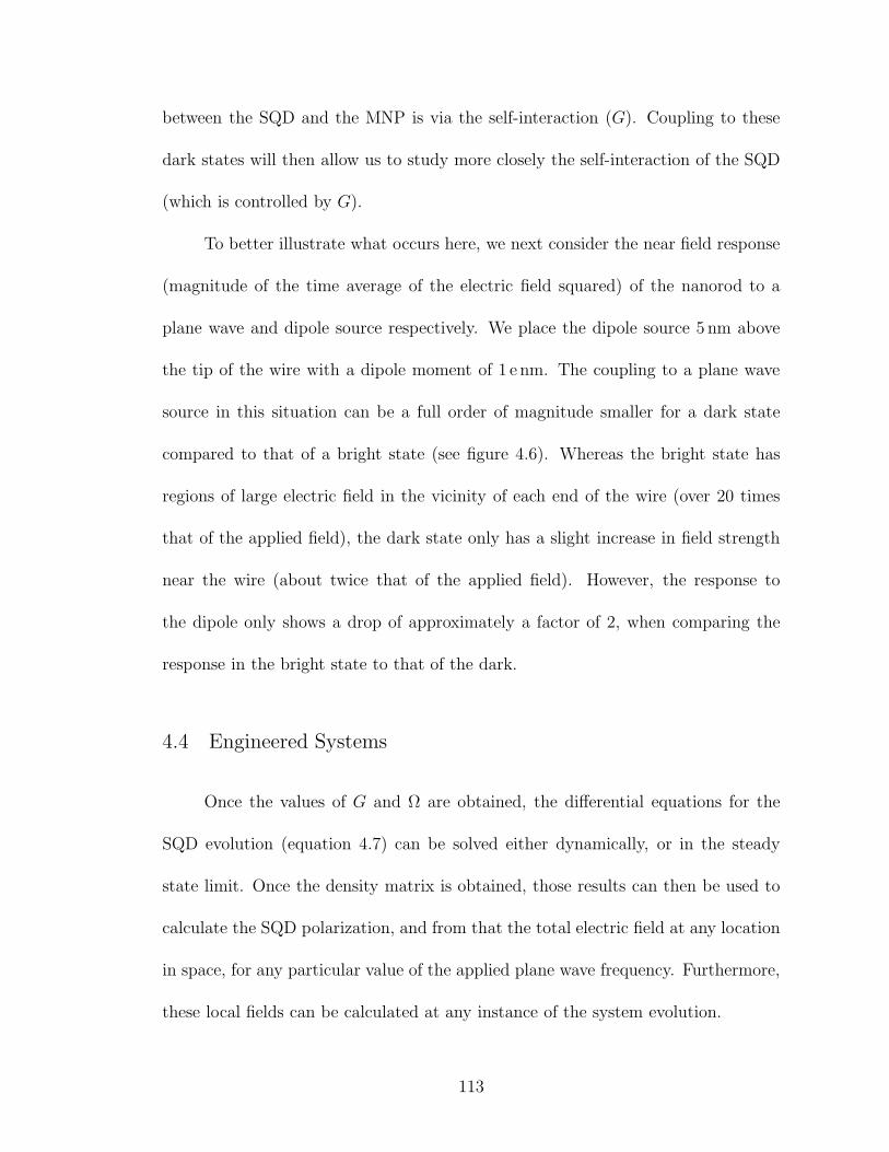
between the SQD and the MNP is via the self-interaction (G). Coupling to these
dark states will then allow us to study more closely the self-interaction of the SQD
(which is controlled by G).
To better illustrate what occurs here, we next consider the near field response
(magnitude of the time average of the electric field squared) of the nanorod to a
plane wave and dipole source respectively. We place the dipole source 5 nm above
the tip of the wire with a dipole moment of 1 e nm. The coupling to a plane wave
source in this situation can be a full order of magnitude smaller for a dark state
compared to that of a bright state (see figure 4.6). Whereas the bright state has
regions of large electric field in the vicinity of each end of the wire (over 20 times
that of the applied field), the dark state only has a slight increase in field strength
near the wire (about twice that of the applied field). However, the response to
the dipole only shows a drop of approximately a factor of 2, when comparing the
response in the bright state to that of the dark.
4.4 Engineered Systems
Once the values of G and Ω are obtained, the differential equations for the
SQD evolution (equation 4.7) can be solved either dynamically, or in the steady
state limit. Once the density matrix is obtained, those results can then be used to
calculate the SQD polarization, and from that the total electric field at any location
in space, for any particular value of the applied plane wave frequency. Furthermore,
these local fields can be calculated at any instance of the system evolution.
113
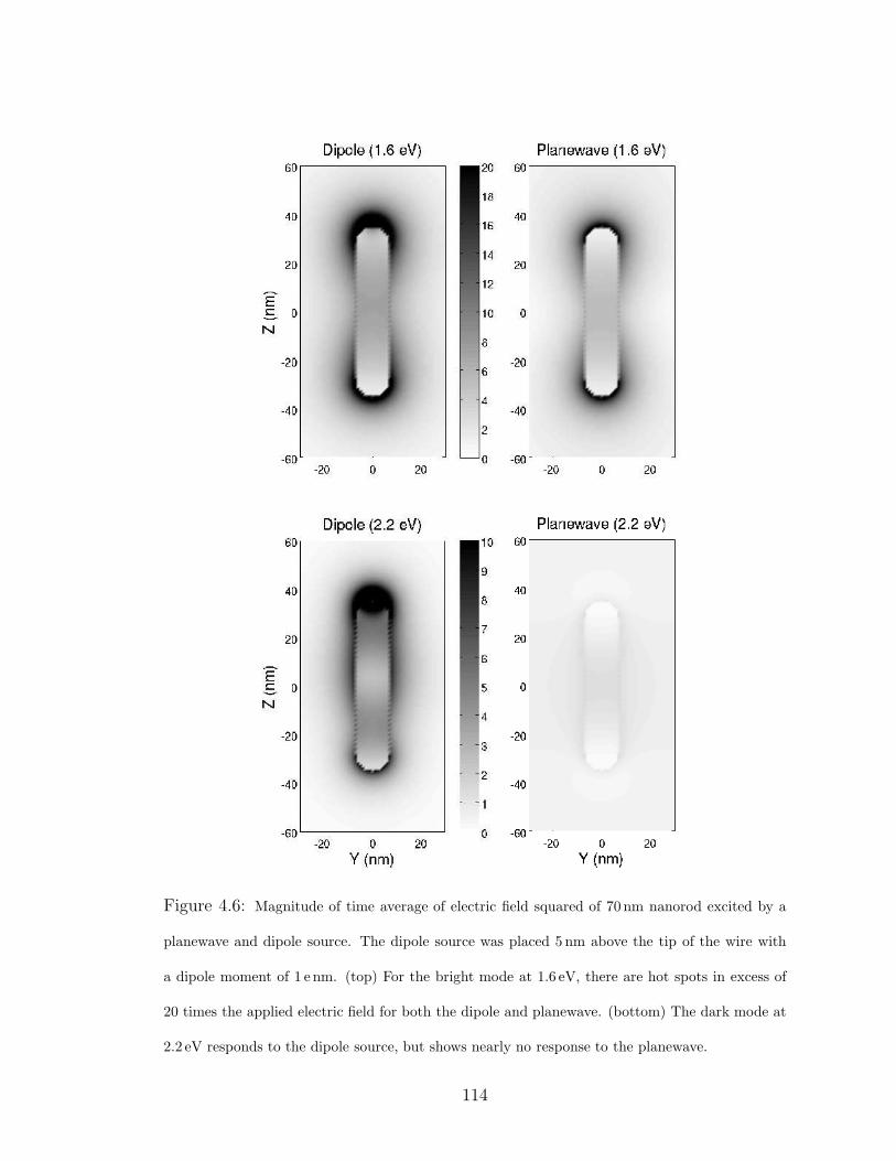
Figure 4.6: Magnitude of time average of electric field squared of 70 nm nanorod excited by a
planewave and dipole source. The dipole source was placed 5 nm above the tip of the wire with
a dipole moment of 1 e nm. (top) For the bright mode at 1.6 eV, there are hot spots in excess of
20 times the applied electric field for both the dipole and planewave. (bottom) The dark mode at
2.2 eV responds to the dipole source, but shows nearly no response to the planewave.
114
0
8
Im[G
] / |
Ω|
1 1.5 2 2.5 3 3.5 4ω (eV)
0
20
|G| /
|Ω|
Figure 4.7: The ratios of GΩ and GIΩ shown for a 70 nm length, 14 nm width nanorod (solid
line) and a 7 nm radius spherical MNP (dashed line), with µ 1.0 enm. These two ratios play a
large role in determining the system behavior.
4.4.1 Dynamics of a 70 nm Nanorod
Last chapter, we showed that by varying the SQD dipole moment and the
radius of a spherical MNP, a large variety of system behavior is achievable. How-
ever, to reach the regimes of strongest coupling, relatively large values of the SQD
dipole moment were needed, µ ¡ 3 enm (see Figure 3.2 in chapter 3). Such large
values of the SQD dipole moment might not be experimentally possible due to the
limit imposed by the SQD size and the relationship of SQD size to the exciton res-
onance. We will show for a nanorod rather than a spherical MNP, that the large
local response of the wire makes the strong coupling regime accessible for smaller
SQD dipole moments that are much more experimentally viable.
Here we illustrate a paradigm for designing systems biased towards specific
115
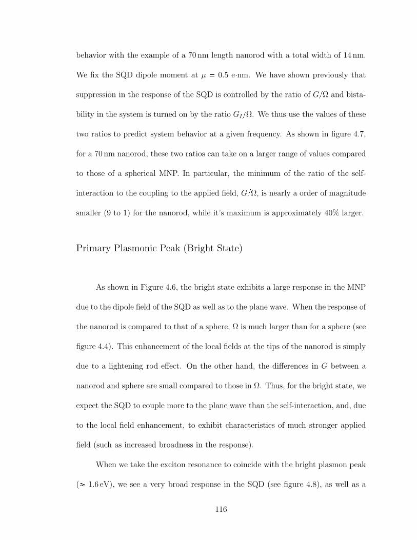
behavior with the example of a 70 nm length nanorod with a total width of 14 nm.
We fix the SQD dipole moment at µ 0.5 enm. We have shown previously that
suppression in the response of the SQD is controlled by the ratio of GΩ and bista-
bility in the system is turned on by the ratio GIΩ. We thus use the values of these
two ratios to predict system behavior at a given frequency. As shown in figure 4.7,
for a 70 nm nanorod, these two ratios can take on a larger range of values compared
to those of a spherical MNP. In particular, the minimum of the ratio of the self-
interaction to the coupling to the applied field, GΩ, is nearly a order of magnitude
smaller (9 to 1) for the nanorod, while it’s maximum is approximately 40% larger.
Primary Plasmonic Peak (Bright State)
As shown in Figure 4.6, the bright state exhibits a large response in the MNP
due to the dipole field of the SQD as well as to the plane wave. When the response of
the nanorod is compared to that of a sphere, Ω is much larger than for a sphere (see
figure 4.4). This enhancement of the local fields at the tips of the nanorod is simply
due to a lightening rod effect. On the other hand, the differences in G between a
nanorod and sphere are small compared to those in Ω. Thus, for the bright state, we
expect the SQD to couple more to the plane wave than the self-interaction, and, due
to the local field enhancement, to exhibit characteristics of much stronger applied
field (such as increased broadness in the response).
When we take the exciton resonance to coincide with the bright plasmon peak
( 1.6 eV), we see a very broad response in the SQD (see figure 4.8), as well as a
116
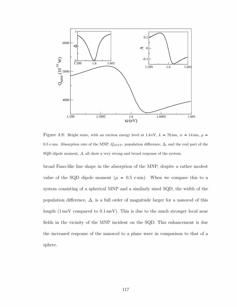
1.599 1.6 1.6010
1
∆
1.599 1.6 1.601
-0.1
0
0.1
A
1.599 1.5995 1.6 1.6005 1.601ω (eV)
4000
5000
6000
QM
NP (
10-1
0 W)
Figure 4.8: Bright state, with an exciton energy level at 1.6 eV, L 70 nm, w 14 nm, µ 0.5 enm. Absorption rate of the MNP, QMNP , population difference, ∆, and the real part of the
SQD dipole moment, A, all show a very strong and broad response of the system.
broad Fano-like line shape in the absorption of the MNP, despite a rather modest
value of the SQD dipole moment (µ 0.5 enm). When we compare this to a
system consisting of a spherical MNP and a similarly sized SQD, the width of the
population difference, ∆, is a full order of magnitude larger for a nanorod of this
length (1meV compared to 0.1meV). This is due to the much stronger local near
fields in the vicinity of the MNP incident on the SQD. This enhancement is due
the increased response of the nanorod to a plane wave in comparison to that of a
sphere.
117
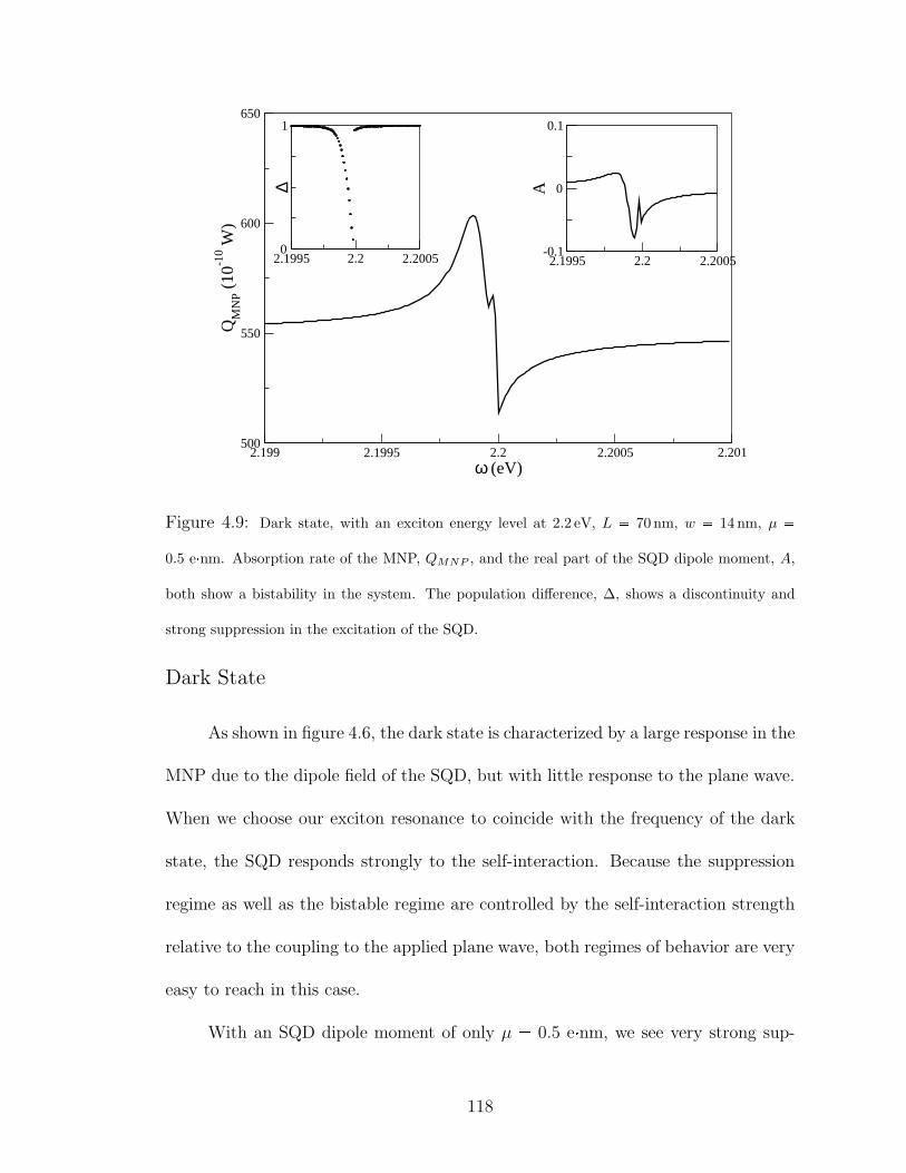
2.1995 2.2 2.20050
1
∆2.1995 2.2 2.2005
-0.1
0
0.1
A
2.199 2.1995 2.2 2.2005 2.201ω (eV)
500
550
600
650
QM
NP (
10-1
0 W)
Figure 4.9: Dark state, with an exciton energy level at 2.2 eV, L 70 nm, w 14 nm, µ 0.5 enm. Absorption rate of the MNP, QMNP , and the real part of the SQD dipole moment, A,
both show a bistability in the system. The population difference, ∆, shows a discontinuity and
strong suppression in the excitation of the SQD.
Dark State
As shown in figure 4.6, the dark state is characterized by a large response in the
MNP due to the dipole field of the SQD, but with little response to the plane wave.
When we choose our exciton resonance to coincide with the frequency of the dark
state, the SQD responds strongly to the self-interaction. Because the suppression
regime as well as the bistable regime are controlled by the self-interaction strength
relative to the coupling to the applied plane wave, both regimes of behavior are very
easy to reach in this case.
With an SQD dipole moment of only µ 0.5 enm, we see very strong sup-
118
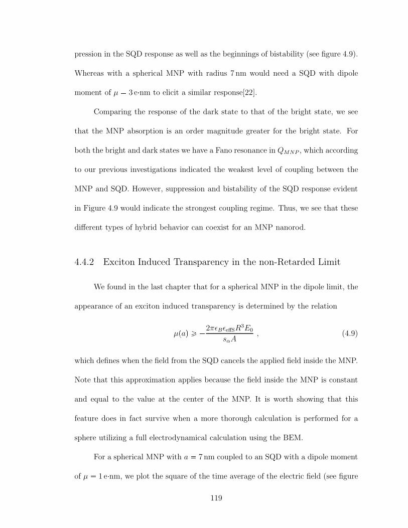
pression in the SQD response as well as the beginnings of bistability (see figure 4.9).
Whereas with a spherical MNP with radius 7 nm would need a SQD with dipole
moment of µ 3 enm to elicit a similar response[22].
Comparing the response of the dark state to that of the bright state, we see
that the MNP absorption is an order magnitude greater for the bright state. For
both the bright and dark states we have a Fano resonance in QMNP , which according
to our previous investigations indicated the weakest level of coupling between the
MNP and SQD. However, suppression and bistability of the SQD response evident
in Figure 4.9 would indicate the strongest coupling regime. Thus, we see that these
different types of hybrid behavior can coexist for an MNP nanorod.
4.4.2 Exciton Induced Transparency in the non-Retarded Limit
We found in the last chapter that for a spherical MNP in the dipole limit, the
appearance of an exciton induced transparency is determined by the relation
µpaq ¥ 2πǫBǫeffSR3E0
sαA, (4.9)
which defines when the field from the SQD cancels the applied field inside the MNP.
Note that this approximation applies because the field inside the MNP is constant
and equal to the value at the center of the MNP. It is worth showing that this
feature does in fact survive when a more thorough calculation is performed for a
sphere utilizing a full electrodynamical calculation using the BEM.
For a spherical MNP with a 7 nm coupled to an SQD with a dipole moment
of µ 1 enm, we plot the square of the time average of the electric field (see figure
119
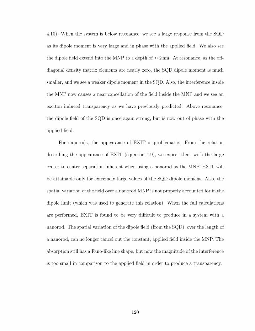
4.10). When the system is below resonance, we see a large response from the SQD
as its dipole moment is very large and in phase with the applied field. We also see
the dipole field extend into the MNP to a depth of 2 nm. At resonance, as the off-
diagonal density matrix elements are nearly zero, the SQD dipole moment is much
smaller, and we see a weaker dipole moment in the SQD. Also, the interference inside
the MNP now causes a near cancellation of the field inside the MNP and we see an
exciton induced transparency as we have previously predicted. Above resonance,
the dipole field of the SQD is once again strong, but is now out of phase with the
applied field.
For nanorods, the appearance of EXIT is problematic. From the relation
describing the appearance of EXIT (equation 4.9), we expect that, with the large
center to center separation inherent when using a nanorod as the MNP, EXIT will
be attainable only for extremely large values of the SQD dipole moment. Also, the
spatial variation of the field over a nanorod MNP is not properly accounted for in the
dipole limit (which was used to generate this relation). When the full calculations
are performed, EXIT is found to be very difficult to produce in a system with a
nanorod. The spatial variation of the dipole field (from the SQD), over the length of
a nanorod, can no longer cancel out the constant, applied field inside the MNP. The
absorption still has a Fano-like line shape, but now the magnitude of the interference
is too small in comparison to the applied field in order to produce a transparency.
120
2.4995 2.5 2.5005ω (eV)
0
100
200
300
QM
NP (
10-1
0 W)
Figure 4.10: Near field of a 5 nm radius spherical MNP interacting with a SQD located 10 nm
away from center for 3 values of applied frequency. Shown in color is the z component of the electric
field. The first plot shows a strong dipole field from the SQD, in-phase with the applied field that
penetrates the MNP to a depth of 2 nm. The middle plot show the system at resonance and the
appearance of the exciton induced transparency in the MNP. The third plot shows a strong dipole
field from the SQD, now out-of-phase with the applied field, that again penetrates the MNP to a
depth of 1 nm.
121
4.5 Concluding Remarks
In this chapter, we have employed a full electrodynamical calculations of the
near fields for MNP-SQD hybrid molecules based on the boundary element method
(BEM). The method allows for tackling more complex geometries with a full de-
scription of the retarded optical response. Fields calculated were compared between
those given by the BEM, those from a multipolar expansion, and those from the
dipole approximation, and we examined the limits which can necessitate such a
treatment.
Calculations performed on systems consisting of an SQD and a nanorod MNP
showed that a broad range of system behavior can be reached experimentally much
more easily than previously thought thanks to the field enhancement from the
nanorod geometry. Furthermore, we saw how the response of the system could
be tailored by engineering metal nanoparticle shape and the SQD resonance to ma-
nipulate the individual local near-fields that couple the MNPs and SQDs.
We also identified regimes where dark modes can influence hybrid response.
Strong local field coupling via dark modes changes the interference and self-interaction
effects dramatically. The external applied field does not directly drive this MNP
dark mode, so SQD-MNP coupling is dominated by the SQD self-interaction. All
of these aspects could enhance the capabilities of metal nanostructures to provide
spatial and spectral control of the optical properties of single emitters.
122
Chapter 5
Multiple SQD Systems
In the previous two chapters we studied systems consisting of a single SQD
coupled to MNPs of various shape. We now turn our attention to the response of a
hybrid nanostructure molecule consisting of two SQDs and a single MNP. In partic-
ular, we will model the system using different approximation techniques. In doing
so, we will identify and address issues in modeling the system using a semiclassical
approach.
We will see that a semiclassical approach in modeling the coupling between
the SQDs can lead to unstable, oscillatory and chaotic behavior in a strong SQD-
SQD coupling regime. This nonlinear behavior is due to a breaking of the identical
particle symmetry. Additionally, we will see that this chaotic behavior is closely
related to the type of decoherence present in the system, specifically, whether the
decoherence is collective or non-collective between the two SQDs. This provides
insight into proper accounting of these important, but often neglected interactions.
We will then model the system using a more quantum mechanical approach,
and note that this chaotic regime is absent. Finally, we will compare the two models
on a system with a strong plasmon-mediated interaction between the SQDs and a
weak direct interaction between them. In this case, we will see that while the results
of the two models are similar, dipole blockade and the level splitting of the single
123
exciton states in the quantum model are non-trivial effects, even in this regime.
The layout of this chapter is as follows. We begin in section 1 with a quick
review of recent work on this and similar systems. In section 2, we look at the
SQD-MNP-SQD molecule in detail and discuss the ways in which we can model
it. In section 3, we use a simple semiclassical approach to model the system and
find a regime of highly chaotic behavior in the case of identical SQDs. We explore
this behavior in detail and see that it is due to a symmetry breaking induced by
non-collective decoherence. Additionally, we find that this chaotic behavior is re-
moved from the system with an increased coupling to the MNP. The coupling to
the classical plasmon of the MNP in this model effectively washes out the nonlinear
effect. In section 4, we replace the semiclassical SQD-SQD direct coupling term with
a quantum mechanical interaction term consistent with molecular quantum electro-
dynamics. In this case, we note the absence of the chaotic behavior. In its place, we
find a dipole blockade induced by the splitting of the symmetric and antisymmetric
SQD eigenstates. We then take a closer look at the dipole blockade and compare
the two models in the weak SQD-SQD coupling regime. Finally, we present our
conclusions in section 5.
5.1 Introduction
Recently, several theoretical investigations have gone beyond the semiclassical
limit in studying this system by treating the plasmon-exciton interaction with quan-
tum mechanical methods, such as treating the plasmon in the quasi-mode formal-
124
ism commonly employed in cavity quantum electrodynamics (QED) [58]. When the
semiclassical results of a single quantum dot interacting with a metal nanoparticle
are compared to a cavity QED treatment, the semiclassical results can be corrected
by properly accounting for dephasing by using a random phase jump method [59].
Also, by using a Green’s function approach to study a system comprised of two
quantum emitters coupled through a nanorod, an optimal emitter-wire separation
for excitation-plasmon conversion was found and plasmon mediated coupling be-
tween the two emitters was studied [60]. In addition to quantizing the local field
produced by the metal particle, progress has been made in better understanding the
inherent quantum properties of very small metal particles, including size quantiza-
tion effects [61, 62] and the plasmon coupling to atomic-scale transport [63].
We discuss here the response of a hybrid nanostructure molecule consisting of
two SQDs and a metal nanoparticle (MNP) subject to an applied electric field. The
field couples to both of the SQDs as well as the MNP and all three constituents
interact with each other through a dipole-dipole coupling. In order to model such
a complex system, a number of approximation schemes must be employed. Differ-
ent choices for the approximations made can result in predictions that differ both
qualitatively and quantitatively. Therefore, a careful examination of the various
techniques that are commonly employed is needed.
Furthermore, with two SQDs being considered as part of an open quantum
system, the nature of the coupling to the bath is of increased importance. Two
identical quantum objects, coupled in phase to the same bath mode, will decohere
collectively. However, a slight detuning of their resonances will introduce a deco-
125
herence in each object independent of the other (and thus non-collective). Coupling
to bath modes internal to each object respectively (exciton-phonon coupling inside
a quantum dot for example [64]) introduces an additional source of non-collective
decoherence. This question of collective vs non-collective decoherence can determine
if and how a particle exchange symmetry can be broken, further complicating the
modeling of the system.
The focus of this chapter is to identify and address these issues in modeling
hybrid systems. Using a semiclassical approach to model the coupling between
the SQDs, we find that such an approximation can lead to unstable, oscillatory and
chaotic behavior in the strong SQD-SQD coupling regime. This nonlinear behavior is
shown to be due to a breaking of the identical particle exchange symmetry. When the
system is modeled using a quantum mechanical model for the SQD-SQD coupling,
this instability is removed. Additionally, we see that this chaotic behavior is closely
related to the type of decoherence present in the system, specifically, whether the
decoherence is collective or non-collective between the two SQDs.
5.2 SQD-MNP-SQD Hybrid Molecule
Consider a hybrid molecule composed of two SQDs with radii r1 and r2 inter-
acting with a spherical MNP of radius a. The MNP is centrally located between the
two SQDs, which are located at distances R1 and R2 respectively from the center of
the MNP (see Figure 5.1). The entire system is subject to an applied electric field
E E0 cospωtq.126
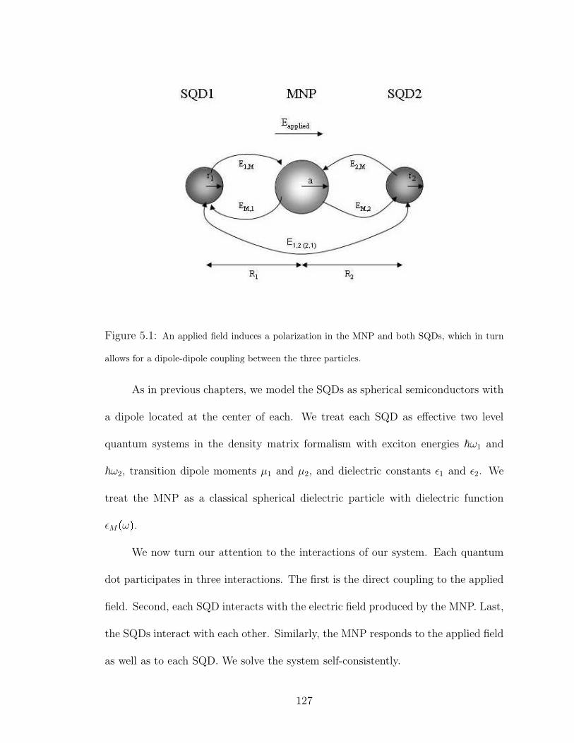
Figure 5.1: An applied field induces a polarization in the MNP and both SQDs, which in turn
allows for a dipole-dipole coupling between the three particles.
As in previous chapters, we model the SQDs as spherical semiconductors with
a dipole located at the center of each. We treat each SQD as effective two level
quantum systems in the density matrix formalism with exciton energies ~ω1 and
~ω2, transition dipole moments µ1 and µ2, and dielectric constants ǫ1 and ǫ2. We
treat the MNP as a classical spherical dielectric particle with dielectric function
ǫMpωq.We now turn our attention to the interactions of our system. Each quantum
dot participates in three interactions. The first is the direct coupling to the applied
field. Second, each SQD interacts with the electric field produced by the MNP. Last,
the SQDs interact with each other. Similarly, the MNP responds to the applied field
as well as to each SQD. We solve the system self-consistently.
127
We begin by writing down the Hamiltonian for the system, Htotal, as
Htotal ~ω1a:1a1 ~ω2a
:2a2 H1Ø2 µ1ESQD1 pa1 a
:1q µ2ESQD2 pa2 a
:2q
where a1p2q and a:1p2q are the exciton annihilation and creation operators for SQD1(2)
and H1Ø2 represents the direct coupling between SQD1 and SQD2. ESQD1 is the
electric field at the center of SQD1 that consists of the applied, external field, E,
and the induced field produced by the polarization of the MNP, EM,1. Thus ESQD1
is
ESQD1 1
ǫeff1pE EM,1q , (5.1)
where ǫeff1 2ǫBǫ13ǫB
is the screening factor of SQD1. The field on SQD1 from the
MNP is
EM,1 1
4πǫB
sαPMNP
R31
, (5.2)
where sα 2p1q when the applied field is parallel (perpendicular) to the major
axis of the system, (ESQD2 is calculated similarly).
As before, working in the dipole limit, the polarization of the MNP is (see
[54]),
PMNP p4πǫBqγa3pE 1
4πǫB
sαPSQD1
ǫeff1R31 1
4πǫB
sαPSQD2
ǫeff2R32
qwhere γ ǫM pωqǫB
2ǫBǫM pωq . Making use of the density matrix ρ to calculate the polarization
of the SQD, we take the ensemble average of the dipole moment. We take as our
states |1〉 |00〉, |2〉 |10〉, |3〉 |01〉 and |4〉 |11〉 (where, for example, |10〉128
is the state with SQD1 excited and SQD2 in its ground state). We then have
PSQD1 µ1pρ12 ρ21 ρ34 ρ43q and PSQD2 µ2pρ13 ρ31 ρ24 ρ42q(see [48]).
This allows us to write down ESQD1, but we still need an expression for H1Ø2 in
order to complete our calculation of Htotal.
5.2.1 The SQD-SQD Interaction
We have several choices for the SQD-SQD coupling terms in our Hamiltonian.
If we treat the field produced by the SQD1 as a classical electric field produced by
a dipole with polarization, PSQD1 µ1pρ12 ρ21 ρ34 ρ43q (similarly for SQD2),
as we did in treating SQD-MNP interactions, then we have
H1Ø2 µ1~E2Ñ1pa1 a
:1q µ2
~E1Ñ2pa2 a:2q
H1Ø2 µ1
1
4πǫB
sαPSQD2
ǫeff2ǫeff1pR1 R2q3 pa1 a:1q µ2
1
4πǫB
sαPSQD1
ǫeff1ǫeff2pR1 R2q3 pa2 a:2q .
In taking this approach, we are assuming that we can replace a quantized field,
produced by the exciton, with a mean field value computed by the density matrix.
This is a semiclassical approximation.
Alternatively, we can calculate this interaction with quantum electrodynamics.
Two identical, two-level molecules interacting with a common electromagnetic mode,
with a radiative decay rate, γ 1τ, separated by a distance d, have an interaction
Hamiltonian of the form [65]
H1Ø2 ~ δ pa1 a:1q pa2 a
:2q , (5.3)
129
where δ, the interaction energy, is calculated in the dipole limit as
δ 3
4τ
cos2pθq 1
cospζqζ 1 3 cos2pθqcospζq
ζ3 sinpζq
ζ2
,
where ζ ωdc, c is the speed of light, and θ denotes the phase difference of the bath
mode at the locations of the two molecules.
5.2.2 Numerical Calculations
Similar to previous chapters, we take E parallel to the axis of our SQD-MNP-
SQD molecule (unless otherwise noted) i.e., sα 2, and we take the dielectric
constant of the background to be ǫB ǫ0. For the MNP, we take ǫMpωq as the
bulk dielectric constant of gold as found experimentally [55]. For a small, spherical,
gold MNP, the response has a broad plasmon peak near 2.4 eV with a width of
approximately 0.25 eV. We let the radius of the MNP vary between 3 and 8 nm.
For the SQDs, we take ǫ1 ǫ2 6 ǫ0 and for the exciton resonant frequency
we take it to be 2.5 eV, which is near the broad plasmon frequency of gold. For the
MNP size regime we consider, the plasmon resonance for a sphere varies little with
particle size. However, the size, shape and material of the SQD strongly determine
both the exciton energy level and its dipole moment. In this chapter, we again
consider the simplest model and ignore this size dependence.
130
5.3 Semiclassical Approach to SQD-SQD coupling
We first model the system using the semiclassical approximation for the SQD-
SQD coupling. Our Hamiltonian becomes
Htotal ~ω1a:1a1 ~ω2a
:2a2 2~ cosωt Ω1 pa1 a
:1q 2~ cosωt Ω2 pa2 a
:2q ~G1pρ12 ρ21 ρ34 ρ43q pa1 a
:1q ~G2pρ13 ρ31 ρ24 ρ42q pa2 a:2q ~F pρ12 ρ21 ρ34 ρ43q pa2 a:2q ~F pρ13 ρ31 ρ24 ρ42q pa1 a:1q
where, similar to previous chapters, we define
G1 γa3µ21s
2α
4πǫB ǫeff1 ~R61
Ω1 E0µ1
2~p1 γa3sα
ǫeffMR31
qF µ1µ2s
2α
4πǫB ǫeff1 ǫeff2 ~
1pR1 R2q3 γa3
R31R
32
,
and G2 and Ω2 are defined similarly. G1 arises when the applied field polarizes
SQD1, which in turn polarizes the MNP and then produces a field to interact back
on SQD1. This can be thought of as the self-interaction of SQD1 because this
coupling to SQD1 depends on the polarization of SQD1. The first term in Ω1 is just
the direct coupling to the applied field and the second term is the field from the
MNP that is induced by the applied field. F arises from the interaction between the
two dots. The first term is the direct coupling and the second term is the interaction
131
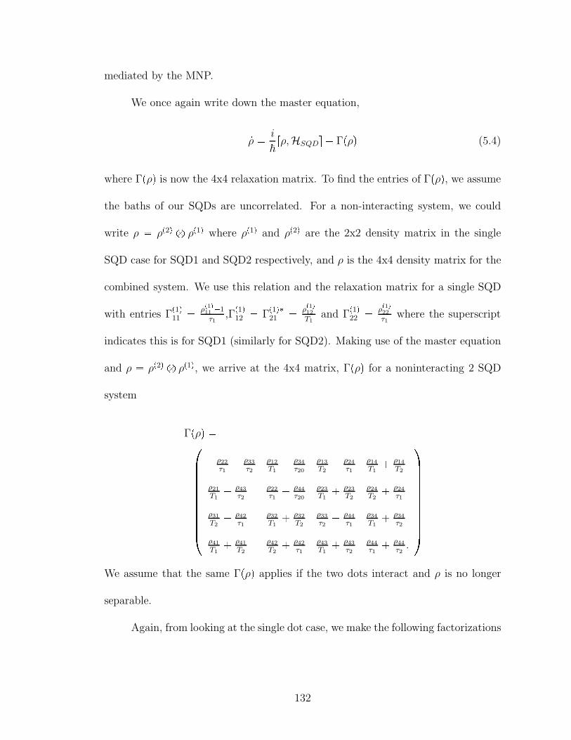
mediated by the MNP.
We once again write down the master equation,9ρ i
~rρ,HSQDs Γpρq (5.4)
where Γpρq is now the 4x4 relaxation matrix. To find the entries of Γpρq, we assume
the baths of our SQDs are uncorrelated. For a non-interacting system, we could
write ρ ρp2q b ρp1q where ρp1q and ρp2q are the 2x2 density matrix in the single
SQD case for SQD1 and SQD2 respectively, and ρ is the 4x4 density matrix for the
combined system. We use this relation and the relaxation matrix for a single SQD
with entries Γp1q11 ρ
p1q11 1
τ1,Γp1q12 Γ
p1q21 ρ
p1q12
T1and Γ
p1q22 ρ
p1q22
τ1where the superscript
indicates this is for SQD1 (similarly for SQD2). Making use of the master equation
and ρ ρp2q b ρp1q, we arrive at the 4x4 matrix, Γpρq for a noninteracting 2 SQD
system
Γpρq ρ22
τ1 ρ33
τ2
ρ12T1
ρ34τ20
ρ13T2
ρ24τ1
ρ14T1 ρ14
T2
ρ21T1 ρ43
τ2
ρ22τ1 ρ44
τ20
ρ23T1
ρ23T2
ρ24T2 ρ24
τ1
ρ31T2 ρ42
τ1
ρ32T1
ρ32T2
ρ33τ2 ρ44
τ1
ρ34T1 ρ34
τ2
ρ41T1 ρ41
T2
ρ42T2
ρ42τ1
ρ43T1
ρ43τ2
ρ44τ1 ρ44
τ2.
ÆÆÆÆÆÆÆÆÆÆ We assume that the same Γpρq applies if the two dots interact and ρ is no longer
separable.
Again, from looking at the single dot case, we make the following factorizations
132
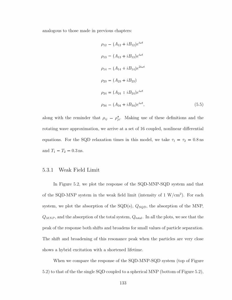
analogous to those made in previous chapters:
ρ12 pA12 iB12qeiωtρ13 pA13 iB13qeiωtρ14 pA14 iB14qe2iωtρ23 pA23 iB23qρ24 pA24 iB24qeiωtρ34 pA34 iB34qeiωt, (5.5)
along with the reminder that ρij ρji. Making use of these definitions and the
rotating wave approximation, we arrive at a set of 16 coupled, nonlinear differential
equations. For the SQD relaxation times in this model, we take τ1 τ2 0.8 ns
and T1 T2 0.3 ns.
5.3.1 Weak Field Limit
In Figure 5.2, we plot the response of the SQD-MNP-SQD system and that
of the SQD-MNP system in the weak field limit (intensity of 1 W/cm2). For each
system, we plot the absorption of the SQD(s), QSQD, the absorption of the MNP,
QMNP , and the absorption of the total system, Qtotal. In all the plots, we see that the
peak of the response both shifts and broadens for small values of particle separation.
The shift and broadening of this resonance peak when the particles are very close
shows a hybrid excitation with a shortened lifetime.
When we compare the response of the SQD-MNP-SQD system (top of Figure
5.2) to that of the the single SQD coupled to a spherical MNP (bottom of Figure 5.2),
133
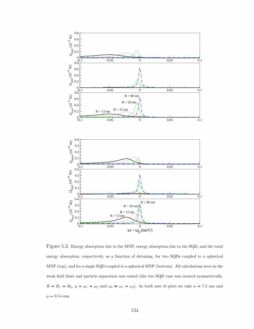
-0.1 -0.05 0 0.05 0.10
0.2
0.4
0.6
0.8
QM
NP (
10-1
0 W)
-0.1 -0.05 0 0.05 0.10
0.2
0.4
0.6
0.8
QSQ
D (
10-1
0 W)
-0.1 -0.05 0 0.05 0.1ω − ω0 (meV)
0
0.2
0.4
0.6
0.8
Qto
tal (
10-1
0 W)
R = 13 nm R = 15 nm
R = 20 nm
R = 80 nm
-0.1 -0.05 0 0.05 0.10
0.1
0.2
0.3
0.4
QM
NP (
10-1
0 W)
-0.1 -0.05 0 0.05 0.10
0.1
0.2
0.3
0.4
QSQ
D (
10-1
0 W)
-0.1 -0.05 0 0.05 0.1ω − ω0 (meV)
0
0.1
0.2
0.3
0.4
Qto
tal (
10-1
0 W)
R = 13 nmR = 15 nm
R = 20 nmR = 80 nm
Figure 5.2: Energy absorption due to the MNP, energy absorption due to the SQD, and the total
energy absorption, respectively, as a function of detuning, for two SQDs coupled to a spherical
MNP (top), and for a single SQD coupled to a spherical MNP (bottom). All calculations were in the
weak field limit and particle separation was varied (the two SQD case was treated symmetrically,
R R1 R2, µ µ1 µ2 and ω0 ω1 ω2). In both sets of plots we take a 7.5 nm and
µ 0.5 enm.
134
we find an overall enhancement of the interaction. We first note that the magnitude
of the absorption is nearly doubled when compared to the single SQD case for most
particle separations. When the particles are far apart, the interparticle coupling is
weak, and most of the absorption is due to the SQDs. Thus, the doubling is simply
the absorption of the additional SQD. When the particles are close together, the
interparticle coupling is strong and most of the absorption is in the MNP. The peak
of the absorption in this case is due to the constructive interference of fields at the
MNP, from the SQDs. Thus, the additional SQD doubles the magnitude of this
field.
In addition to enhancing the magnitude of the absorption, we also have an
increase in the interparticle coupling strength. This is evident in the increased
shifting and slight broadening of the response, for a given R, when compared to
the single SQD case. This shifting of the resonance indicates that a smaller particle
separation is needed in the single SQD-MNP molecule than in the SQD-MNP-SQD
system to achieve a similar hybrid response.
5.3.2 Strong Field Limit: a vs. µ Parameter Space
We now consider the large field limit as previously defined [20] (intensity of
103 W/cm2). As we did previously, by manipulating a and µ (µ µ1 µ2), which
are effectively the sizes of the MNP and the SQDs, we can change the relative
strengths of the local fields and, in turn, the strengths of the five different couplings
(G, and the two terms that make up each of Ω and F ). Looking at the solutions to
135
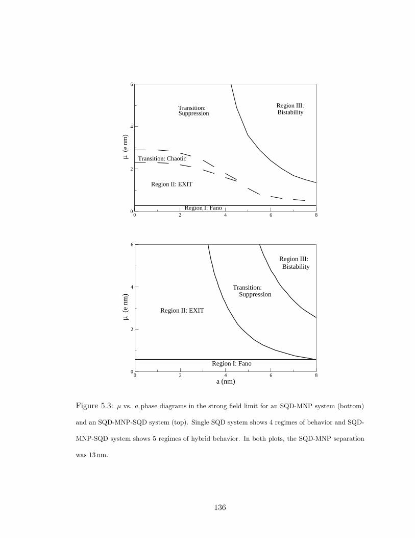
0 2 4 6 8a (nm)
0
2
4
6
µ (
e nm
)
Region II: EXIT
Region I: Fano
Region III:Transition:
Transition: Chaotic
BistabilitySuppression
0 2 4 6 8a (nm)
0
2
4
6
µ (
e nm
)
Region II: EXIT
Region I: Fano
Region III:
Suppression
Bistability
Transition:
Figure 5.3: µ vs. a phase diagrams in the strong field limit for an SQD-MNP system (bottom)
and an SQD-MNP-SQD system (top). Single SQD system shows 4 regimes of behavior and SQD-
MNP-SQD system shows 5 regimes of hybrid behavior. In both plots, the SQD-MNP separation
was 13 nm.
136
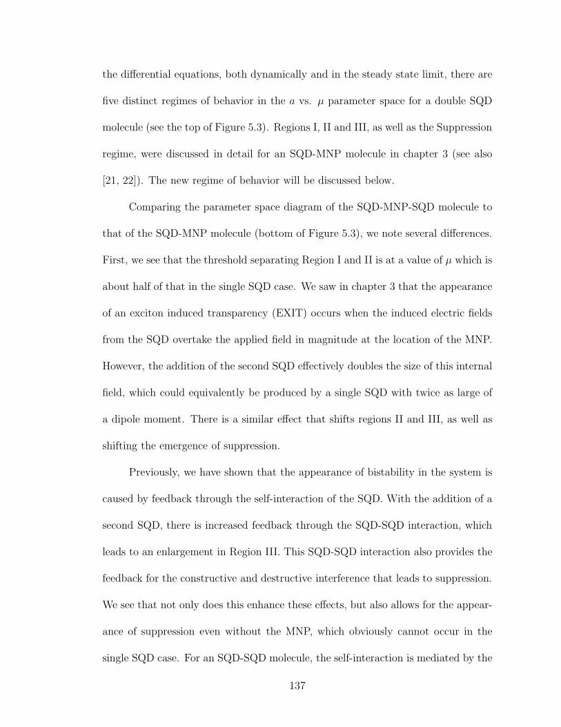
the differential equations, both dynamically and in the steady state limit, there are
five distinct regimes of behavior in the a vs. µ parameter space for a double SQD
molecule (see the top of Figure 5.3). Regions I, II and III, as well as the Suppression
regime, were discussed in detail for an SQD-MNP molecule in chapter 3 (see also
[21, 22]). The new regime of behavior will be discussed below.
Comparing the parameter space diagram of the SQD-MNP-SQD molecule to
that of the SQD-MNP molecule (bottom of Figure 5.3), we note several differences.
First, we see that the threshold separating Region I and II is at a value of µ which is
about half of that in the single SQD case. We saw in chapter 3 that the appearance
of an exciton induced transparency (EXIT) occurs when the induced electric fields
from the SQD overtake the applied field in magnitude at the location of the MNP.
However, the addition of the second SQD effectively doubles the size of this internal
field, which could equivalently be produced by a single SQD with twice as large of
a dipole moment. There is a similar effect that shifts regions II and III, as well as
shifting the emergence of suppression.
Previously, we have shown that the appearance of bistability in the system is
caused by feedback through the self-interaction of the SQD. With the addition of a
second SQD, there is increased feedback through the SQD-SQD interaction, which
leads to an enlargement in Region III. This SQD-SQD interaction also provides the
feedback for the constructive and destructive interference that leads to suppression.
We see that not only does this enhance these effects, but also allows for the appear-
ance of suppression even without the MNP, which obviously cannot occur in the
single SQD case. For an SQD-SQD molecule, the self-interaction is mediated by the
137
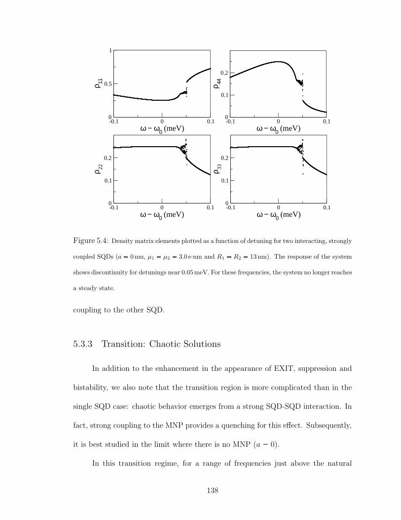
-0.1 0 0.1ω − ω0 (meV)
0
0.1
0.2
ρ 33
-0.1 0 0.1ω − ω0 (meV)
0
0.1
0.2
ρ 22
-0.1 0 0.1ω − ω0 (meV)
0
0.5
1
ρ 11
-0.1 0 0.1ω − ω0 (meV)
0
0.1
0.2
ρ 44
Figure 5.4: Density matrix elements plotted as a function of detuning for two interacting, strongly
coupled SQDs (a 0 nm, µ1 µ2 3.0 enm and R1 R2 13nm). The response of the system
shows discontinuity for detunings near 0.05meV. For these frequencies, the system no longer reaches
a steady state.
coupling to the other SQD.
5.3.3 Transition: Chaotic Solutions
In addition to the enhancement in the appearance of EXIT, suppression and
bistability, we also note that the transition region is more complicated than in the
single SQD case: chaotic behavior emerges from a strong SQD-SQD interaction. In
fact, strong coupling to the MNP provides a quenching for this effect. Subsequently,
it is best studied in the limit where there is no MNP (a 0).
In this transition regime, for a range of frequencies just above the natural
138
resonance of the SQDs, the system no longer reaches a steady state (see Figure
5.4). In this frequency range (ω ω0 35 50µeV with ω0 ω1 ω2, for
a 0 nm, µ1 µ2 3.0 enm and R1 R2 13 nm), the solutions oscillate
within a narrow envelope. We also note that despite the symmetry between the two
SQDs, the population densities for the singly excited SQD states, ρ22 and ρ33, are no
longer identical for these solutions. Thus, we speculate that noise in the numerical
calculations causes the symmetry to be broken. In fact, when the calculations
are performed with increasingly greater numerical precision, much of this chaotic
behavior can be eliminated. However, in all calculations performed, it could never
be removed completely and the numerical precision required (less than 1 part in
1010) far exceeded the amount of natural noise a realistic system would exhibit by
many orders of magnitude.
5.3.3.1 Explicit Symmetry Breaking
In order to explore the effect of the SQD-SQD identical particle symmetry, we
look at the effect of breaking it explicitly. Again, this can best be done without
the presence of the MNP, and by slightly shifting the dipole moment, or the bare
resonance frequency of one of the SQDs. However, care must be taken when detuning
the SQD resonances as too large of a shift could cause them to uncouple.
When the SQD-SQD symmetry is broken explicitly, the chaotic behavior is
amplified. Shown in Figure 5.5 is the response of the system under four different
cases of symmetry breaking. If we compare the responses shown in Figure 5.5 to
139
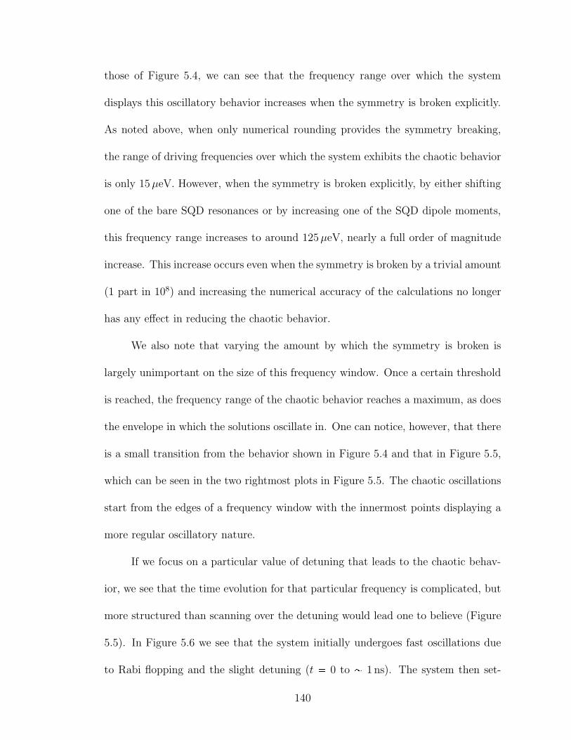
those of Figure 5.4, we can see that the frequency range over which the system
displays this oscillatory behavior increases when the symmetry is broken explicitly.
As noted above, when only numerical rounding provides the symmetry breaking,
the range of driving frequencies over which the system exhibits the chaotic behavior
is only 15µeV. However, when the symmetry is broken explicitly, by either shifting
one of the bare SQD resonances or by increasing one of the SQD dipole moments,
this frequency range increases to around 125µeV, nearly a full order of magnitude
increase. This increase occurs even when the symmetry is broken by a trivial amount
(1 part in 108) and increasing the numerical accuracy of the calculations no longer
has any effect in reducing the chaotic behavior.
We also note that varying the amount by which the symmetry is broken is
largely unimportant on the size of this frequency window. Once a certain threshold
is reached, the frequency range of the chaotic behavior reaches a maximum, as does
the envelope in which the solutions oscillate in. One can notice, however, that there
is a small transition from the behavior shown in Figure 5.4 and that in Figure 5.5,
which can be seen in the two rightmost plots in Figure 5.5. The chaotic oscillations
start from the edges of a frequency window with the innermost points displaying a
more regular oscillatory nature.
If we focus on a particular value of detuning that leads to the chaotic behav-
ior, we see that the time evolution for that particular frequency is complicated, but
more structured than scanning over the detuning would lead one to believe (Figure
5.5). In Figure 5.6 we see that the system initially undergoes fast oscillations due
to Rabi flopping and the slight detuning (t 0 to 1 ns). The system then set-
140
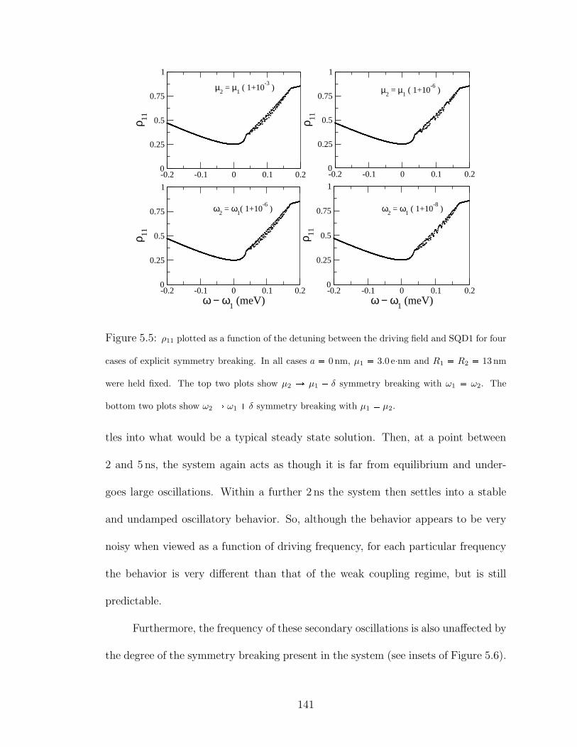
-0.2 -0.1 0 0.1 0.20
0.25
0.5
0.75
1
ρ 11
-0.2 -0.1 0 0.1 0.20
0.25
0.5
0.75
1
ρ 11
-0.2 -0.1 0 0.1 0.2ω − ω
1 (meV)
0
0.25
0.5
0.75
1
ρ 11
-0.2 -0.1 0 0.1 0.2ω − ω
1 (meV)
0
0.25
0.5
0.75
1
ρ 11
µ2 = µ
1 ( 1+10
-3 ) µ
2 = µ
1 ( 1+10
-6 )
ω2 = ω
1( 1+10
-6 ) ω
2 = ω
1 ( 1+10
-8 )
Figure 5.5: ρ11 plotted as a function of the detuning between the driving field and SQD1 for four
cases of explicit symmetry breaking. In all cases a 0 nm, µ1 3.0 enm and R1 R2 13 nm
were held fixed. The top two plots show µ2 Ñ µ1 δ symmetry breaking with ω1 ω2. The
bottom two plots show ω2 Ñ ω1 δ symmetry breaking with µ1 µ2.
tles into what would be a typical steady state solution. Then, at a point between
2 and 5 ns, the system again acts as though it is far from equilibrium and under-
goes large oscillations. Within a further 2 ns the system then settles into a stable
and undamped oscillatory behavior. So, although the behavior appears to be very
noisy when viewed as a function of driving frequency, for each particular frequency
the behavior is very different than that of the weak coupling regime, but is still
predictable.
Furthermore, the frequency of these secondary oscillations is also unaffected by
the degree of the symmetry breaking present in the system (see insets of Figure 5.6).
141
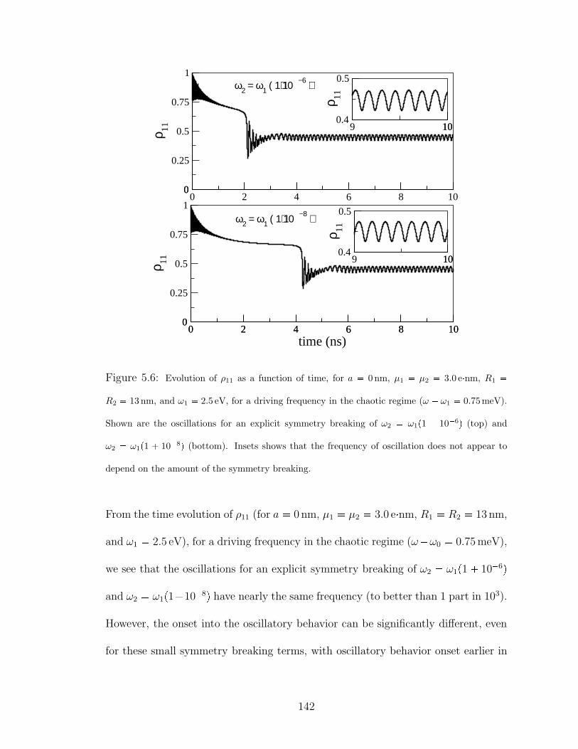
0 2 4 6 8 10time (ns)
0
0.25
0.5
0.75
1
ρ 11
0 2 4 6 8 100
9 100.4
0.5
ρ 11
10
0
0.25
0.5
0.75
1
ρ 11
0 2 4 6 8 100
9 100.4
0.5
ρ 11
10
ω2 = ω1 ( 1+ 10−6 )
ω2 = ω1 ( 1+ 10−8 )
Figure 5.6: Evolution of ρ11 as a function of time, for a 0 nm, µ1 µ2 3.0 enm, R1 R2 13 nm, and ω1 2.5 eV, for a driving frequency in the chaotic regime (ω ω1 0.75meV).
Shown are the oscillations for an explicit symmetry breaking of ω2 ω1p1 106q (top) and
ω2 ω1p1 108q (bottom). Insets shows that the frequency of oscillation does not appear to
depend on the amount of the symmetry breaking.
From the time evolution of ρ11 (for a 0 nm, µ1 µ2 3.0 enm, R1 R2 13 nm,
and ω1 2.5 eV), for a driving frequency in the chaotic regime (ωω0 0.75meV),
we see that the oscillations for an explicit symmetry breaking of ω2 ω1p1 106qand ω2 ω1p1108q have nearly the same frequency (to better than 1 part in 103).
However, the onset into the oscillatory behavior can be significantly different, even
for these small symmetry breaking terms, with oscillatory behavior onset earlier in
142
0 2 40
0.25
0.5
ρ 22
0 2 40
0.5
ρ SS
0 2 4time (ns)
0
0.25
0.5
ρ 33
0 2 4time (ns)
0
0.5
ρ AA
Figure 5.7: Time evolution of ρ22, ρ33, ρSS and ρAA, for a 0 nm, µ1 µ2 3.0 enm,
R1 R2 13 nm, ω1 2.5 eV and ω2 ω1p1 106q, for a driving frequency in the chaotic
regime (ω ω1 0.75meV). ρ22, ρ33, and ρSS are initially driven and quickly oscillate, while ρAA
slowly fills due to relaxation.
the case of the larger symmetry breaking (2 ns compared to 4 ns). This remains the
case even for increasingly large symmetry breaking.
5.3.3.2 The symmetric-antisymmetric basis
We now focus on the behavior of the two individual SQDs in this chaotic regime
by looking at the probabilities that each SQD is excited (ρ22 and ρ33 respectively).
In the absence of the MNP, with µ1 µ2 3.0 enm, R1 R2 13 nm, ω1 2.5 eV
and ω2 ω1p1 108q, and for a driving frequency in the chaotic regime (ω ω1 0.75meV), we see that the two SQDs beat out of phase (see Fig 5.7).
143
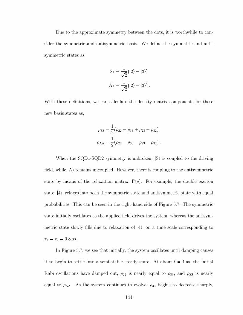
Due to the approximate symmetry between the dots, it is worthwhile to con-
sider the symmetric and antisymmetric basis. We define the symmetric and anti-
symmetric states as |S〉 1?2p|2〉 |3〉q|A〉 1?
2p|2〉 |3〉q .
With these definitions, we can calculate the density matrix components for these
new basis states as,
ρSS 1
2pρ22 ρ33 ρ23 ρ32q
ρAA 1
2pρ22 ρ33 ρ23 ρ32q .
When the SQD1-SQD2 symmetry is unbroken, |S〉 is coupled to the driving
field, while |A〉 remains uncoupled. However, there is coupling to the antisymmetric
state by means of the relaxation matrix, Γpρq. For example, the double exciton
state, |4〉, relaxes into both the symmetric state and antisymmetric state with equal
probabilities. This can be seen in the right-hand side of Figure 5.7. The symmetric
state initially oscillates as the applied field drives the system, whereas the antisym-
metric state slowly fills due to relaxation of |4〉, on a time scale corresponding to
τ1 τ2 0.8 ns.
In Figure 5.7, we see that initially, the system oscillates until damping causes
it to begin to settle into a semi-stable steady state. At about t 1 ns, the initial
Rabi oscillations have damped out, ρ22 is nearly equal to ρ33, and ρSS is nearly
equal to ρAA. As the system continues to evolve, ρ33 begins to decrease sharply,
144
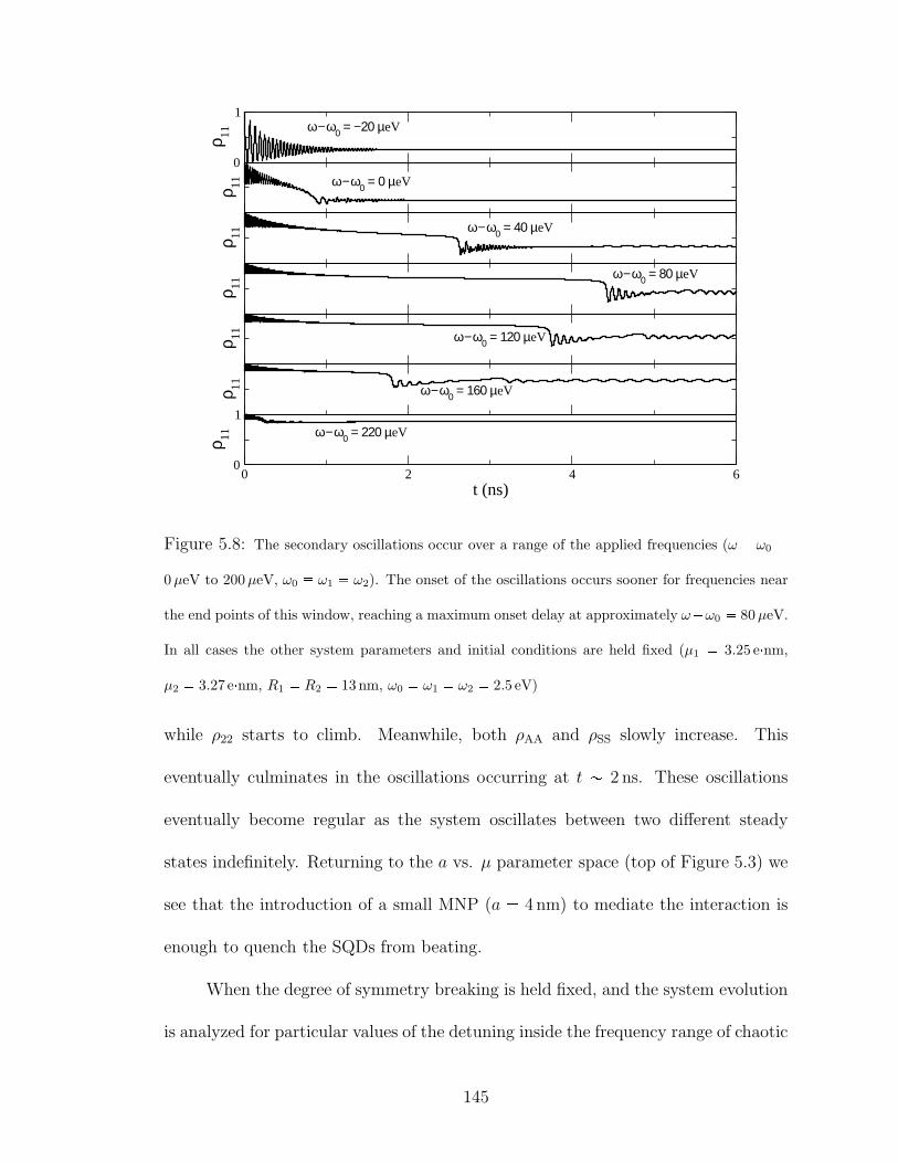
0
1
ρ 11ρ 11
ρ 11ρ 11
ρ 11ρ 11
0 2 4 6t (ns)
0
1
ρ 11
ω−ω0 = 160 µeV
ω−ω0 = 120 µeV
ω−ω0 = 80 µeV
ω−ω0 = 40 µeV
ω−ω0 = 0 µeV
ω−ω0 = −20 µeV
ω−ω0 = 220 µeV
Figure 5.8: The secondary oscillations occur over a range of the applied frequencies (ω ω0 0µeV to 200µeV, ω0 ω1 ω2). The onset of the oscillations occurs sooner for frequencies near
the end points of this window, reaching a maximum onset delay at approximately ωω0 80µeV.
In all cases the other system parameters and initial conditions are held fixed (µ1 3.25 enm,
µ2 3.27 enm, R1 R2 13 nm, ω0 ω1 ω2 2.5 eV)
while ρ22 starts to climb. Meanwhile, both ρAA and ρSS slowly increase. This
eventually culminates in the oscillations occurring at t 2 ns. These oscillations
eventually become regular as the system oscillates between two different steady
states indefinitely. Returning to the a vs. µ parameter space (top of Figure 5.3) we
see that the introduction of a small MNP (a 4 nm) to mediate the interaction is
enough to quench the SQDs from beating.
When the degree of symmetry breaking is held fixed, and the system evolution
is analyzed for particular values of the detuning inside the frequency range of chaotic
145
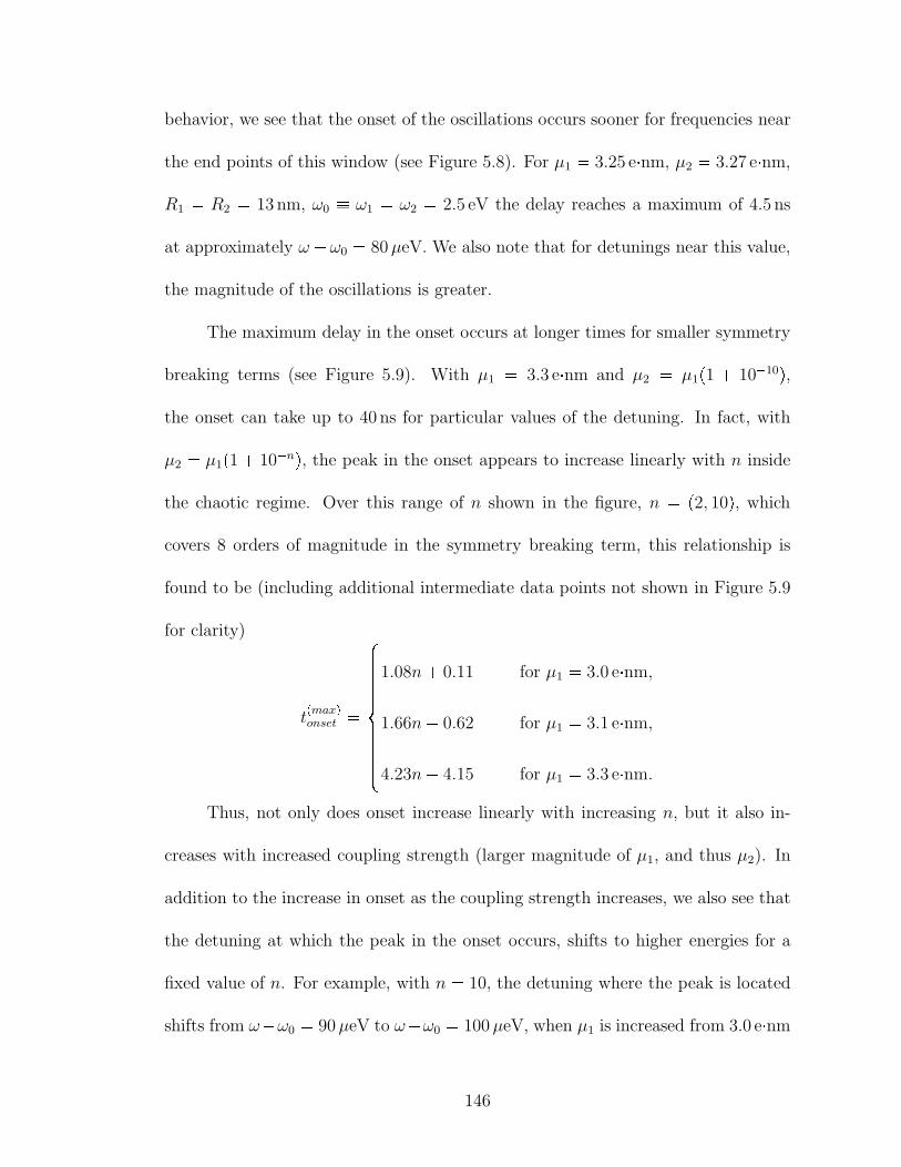
behavior, we see that the onset of the oscillations occurs sooner for frequencies near
the end points of this window (see Figure 5.8). For µ1 3.25 enm, µ2 3.27 enm,
R1 R2 13 nm, ω0 ω1 ω2 2.5 eV the delay reaches a maximum of 4.5 ns
at approximately ω ω0 80µeV. We also note that for detunings near this value,
the magnitude of the oscillations is greater.
The maximum delay in the onset occurs at longer times for smaller symmetry
breaking terms (see Figure 5.9). With µ1 3.3 enm and µ2 µ1p1 1010q,the onset can take up to 40 ns for particular values of the detuning. In fact, with
µ2 µ1p1 10nq, the peak in the onset appears to increase linearly with n inside
the chaotic regime. Over this range of n shown in the figure, n p2, 10q, whichcovers 8 orders of magnitude in the symmetry breaking term, this relationship is
found to be (including additional intermediate data points not shown in Figure 5.9
for clarity)
tpmaxqonset $''''''''&''''''''%
1.08n 0.11 for µ1 3.0 enm,1.66n 0.62 for µ1 3.1 enm,4.23n 4.15 for µ1 3.3 enm.
Thus, not only does onset increase linearly with increasing n, but it also in-
creases with increased coupling strength (larger magnitude of µ1, and thus µ2). In
addition to the increase in onset as the coupling strength increases, we also see that
the detuning at which the peak in the onset occurs, shifts to higher energies for a
fixed value of n. For example, with n 10, the detuning where the peak is located
shifts from ωω0 90µeV to ωω0 100µeV, when µ1 is increased from 3.0 enm146
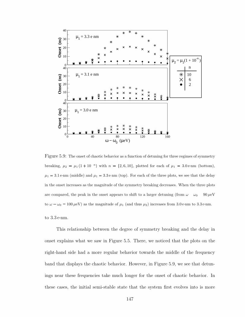
0
10
20
30
40
Ons
et (
ns)
0 40 80 120 160ω − ω0 (µeV)
0
10
20
30
40
Ons
et (
ns)
0
10
20
30
40
Ons
et (
ns)
µ1 = 3.3 e nm
µ1 = 3.1 e nm
µ1 = 3.0 e nm
µ2 = µ1(1 + 10-n
)
n
26
10
Figure 5.9: The onset of chaotic behavior as a function of detuning for three regimes of symmetry
breaking, µ2 µ1 p1 10nq with n t2, 6, 10u, plotted for each of µ1 3.0 enm (bottom),
µ1 3.1 enm (middle) and µ1 3.3 enm (top). For each of the three plots, we see that the delay
in the onset increases as the magnitude of the symmetry breaking decreases. When the three plots
are compared, the peak in the onset appears to shift to a larger detuning (from ω ω0 90µeV
to ω ω0 100µeV) as the magnitude of µ1 (and thus µ2) increases from 3.0 enm to 3.3 enm.
to 3.3 enm.
This relationship between the degree of symmetry breaking and the delay in
onset explains what we saw in Figure 5.5. There, we noticed that the plots on the
right-hand side had a more regular behavior towards the middle of the frequency
band that displays the chaotic behavior. However, in Figure 5.9, we see that detun-
ings near these frequencies take much longer for the onset of chaotic behavior. In
these cases, the initial semi-stable state that the system first evolves into is more
147

stable than for fields driving the system near the edges of the chaotic regime fre-
quency window. Thus, a larger asymmetry must be built up in the system before
the system can be knocked out of this semi-stable state, which accounts for this
additional time.
Since the antisymmetric state is a higher energy state than the symmetric
state, the location of the antisymmetric resonance is above the bare resonance and
is in fact in this chaotic region. Since the interaction term between the two SQDs
is ~F times the transition dipole moment operator, we can estimate the splitting
between the symmetric and antisymmetric state to be 2~F 〈µ〉. For µ1 3.25 enm,
µ2 3.27 enm, R1 R2 13 nm, this splitting is approximately 100µeV, so we
expect the antisymmetric mode to be around ωω1 50µeV which is very close to
the location of the maximum delay in the onset of secondary oscillations. However,
energy splitting and level repulsion between quantum levels is obviously a quantum
effect, thus we can expect that the semiclassical approximation for the SQD-SQD
coupling breaks down here.
5.4 Towards A More Quantum Mechanical Approach
Previously, we took the single SQD relaxation matrix as a basis to construct
the two-particle relaxation matrix in order to model the interaction with the bath.
If we define the Lindblad operator as
LpA, Bq AρB: 1
2
B:Aρ ρB:A , (5.6)
148
then this method is equivalent to taking 4 Lindblad terms, namely, relaxation of
SQD1, Lpa1, a1q, relaxation of SQD2, Lpa2, a2q, dephasing of SQD1, Lpa:1a1, a:1a1q,and dephasing of SQD2, Lpa:2a2, a:2a2q. However, since we are treating the SQDs to
be very closely separated and very near to each other in resonance, they can both in
effect interact with the same bath. For example, both dots would interact with the
same photon modes. As a consequence, spontaneous decay into these modes should
occur due to the coherent response of the two dots (superradiance). Thus, there are
two other Lindblad terms that we should consider, Lpa1, a2q and Lpa2, a1q, i.e., abath-induced interaction between the two dots. If we allow the two SQDs to interact
with the same bath mode, then this should also be reflected in our Hamiltonian.
5.4.1 Quantum Mechanical SQD-SQD Coupling
We now instead use the quantum mechanical expression for the coupling be-
tween the two dots [65]. Our Hamiltonian is then
Htotal ~ω1a:1a1 ~ω2a
:2a2 2~ cosωt Ω1 pa1 a
:1q 2~ cosωt Ω2 pa2 a
:2q ~G1pρ12 ρ21 ρ34 ρ43q pa1 a
:1q ~G2pρ13 ρ31 ρ24 ρ42q pa2 a:2q ~FQMpρ12 ρ21 ρ34 ρ43q pa2 a:2q ~FQMpρ13 ρ31 ρ24 ρ42q pa1 a:1q ~δpa:1a2 a
:2a1q
149
where G and Ω terms are defined as before and FQM is defined as
FQM γa3µ1µ2s2α
4πǫB ǫeff1 ǫeff2 ~R31R
32
. (5.7)
δ was given previously as,
δ 3
4τ
cos2pθq 1
cospζqζ 1 3 cos2pθqcospζq
ζ3 sinpζq
ζ2
where ζ ωd
c, c is the speed of light, and θ denotes the phase difference of the bath
mode at the locations of the two molecules. We still use the semiclassical expression
for the MNP mediated coupling between the dots (FQM), but replace the direct
coupling term with a quantum mechanical form.
To find the relaxation of the system, we now take a more complicated inter-
action Hamiltonian with the reservoir, HR, of the form,
HR λ1a:1b1 λ2a1b:1 λ3a
:2b2 λ4a2b
:2 λ5a
:1a1b
:1b1 λ6a
:2a2b
:2b2 λ7pa:1 a
:2qc λ8pa1 a2qc:, (5.8)
where the bi’s are the operators for the internal bath of each SQD respectively
(for example, coupling to the internal phonon modes of each dot), the c operators
denote the bath processes that are common to both SQDs, and λi’s are yet to
be determined constants. The first 4 terms represent the non-collective portion of
spontaneous emission and excitation, due to a possible symmetry breaking between
the two particles as well as optical phonons inside each SQD. The next two terms
150
are due to scattering and give rise to pure dephasing. We imagine this process to be
dominated by acoustic phonon-electron coupling[64] within each SQD separately,
and thus treat it completely non-collectively. The final two terms represent the
collective portion of spontaneous emission and excitation.
From equation (5.8), we make 6 Lindblad terms, ignoring those generated by
a:1 and a
:2, as they would represent bath induced excitation and we are imagining
our bath to be at a much lower temperature than needed to induce an excitation at
the optical energy scale. We can now write our relaxation matrix asΓ 1
τ1Lpa1, a1q 1
τ2Lpa2, a2q 1
T1Lpa:1a1, a:1a1q 1
T2Lpa:2a2, a:2a2q 1
τcLpa1 a2, a1 a2q.
τc is the collective decoherence and can be calculated with molecular QED. For two
identical particles with a spontaneous decay rate 1τ, then we find τc as
τc 2τ
3
1 cos2pθq sinpζq
ζ 1 3 cos2pθqcospζqζ2
sinpζqζ3
,
with ζ and θ as before.
5.4.2 Numerical Results
Solving the master equation (5.4) with our quantum interaction Hamiltonian,
we find that the system no longer exhibits the behavior of the chaotic regime. For
example, with µ1 3.0 enm, µ2 µ1p1 103q, R1 R2 13 nm, and a=0, the
system shows a broad, smooth response (see Figure 5.10). However, these parameter
151
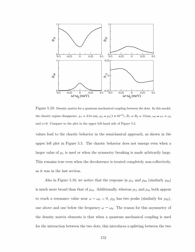
-0.5 -0.25 0 0.25 0.50
1
ρ 11-0.5 -0.25 0 0.25 0.50
1
ρ 22
-0.5 -0.25 0 0.25 0.5ω−ω0 (meV)
0
1
ρ 44
-0.5 -0.25 0 0.25 0.5ω−ω0 (meV)
-0.25
0
0.25
A12
Figure 5.10: Density matrix for a quantum mechanical coupling between the dots. In this model,
the chaotic regime disappears. µ1 3.0 enm, µ2 µ1p1 103q, R1 R2 13 nm, ω0 ω1 ω2
and a=0. Compare to the plot in the upper left-hand side of Figure 5.5.
values lead to the chaotic behavior in the semiclassical approach, as shown in the
upper left plot in Figure 5.5. The chaotic behavior does not emerge even when a
larger value of µ1 is used or when the symmetry breaking is made arbitrarily large.
This remains true even when the decoherence is treated completely non-collectively,
as it was in the last section.
Also in Figure 5.10, we notice that the response in ρ11 and ρ22 (similarly ρ33)
is much more broad than that of ρ44. Additionally, whereas ρ11 and ρ44 both appear
to reach a resonance value near ω ω0 0, ρ22 has two peaks (similarly for ρ33),
one above and one below the frequency ω ω0. The reason for this asymmetry of
the density matrix elements is that when a quantum mechanical coupling is used
for the interaction between the two dots, this introduces a splitting between the two
152
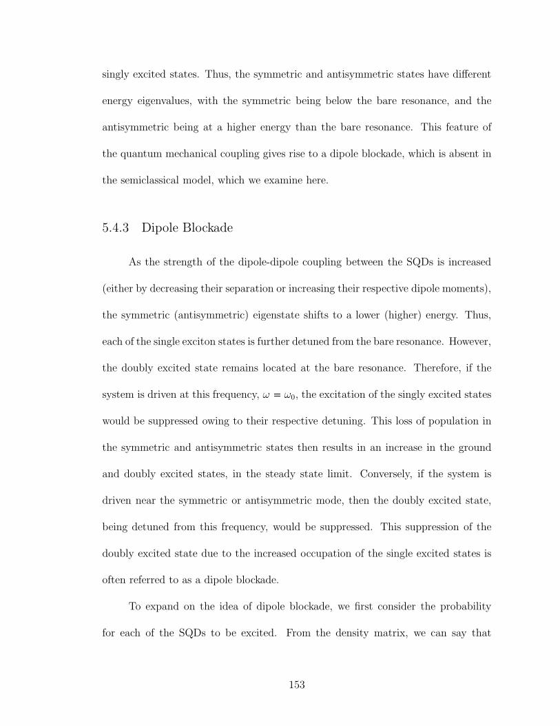
singly excited states. Thus, the symmetric and antisymmetric states have different
energy eigenvalues, with the symmetric being below the bare resonance, and the
antisymmetric being at a higher energy than the bare resonance. This feature of
the quantum mechanical coupling gives rise to a dipole blockade, which is absent in
the semiclassical model, which we examine here.
5.4.3 Dipole Blockade
As the strength of the dipole-dipole coupling between the SQDs is increased
(either by decreasing their separation or increasing their respective dipole moments),
the symmetric (antisymmetric) eigenstate shifts to a lower (higher) energy. Thus,
each of the single exciton states is further detuned from the bare resonance. However,
the doubly excited state remains located at the bare resonance. Therefore, if the
system is driven at this frequency, ω ω0, the excitation of the singly excited states
would be suppressed owing to their respective detuning. This loss of population in
the symmetric and antisymmetric states then results in an increase in the ground
and doubly excited states, in the steady state limit. Conversely, if the system is
driven near the symmetric or antisymmetric mode, then the doubly excited state,
being detuned from this frequency, would be suppressed. This suppression of the
doubly excited state due to the increased occupation of the single excited states is
often referred to as a dipole blockade.
To expand on the idea of dipole blockade, we first consider the probability
for each of the SQDs to be excited. From the density matrix, we can say that
153
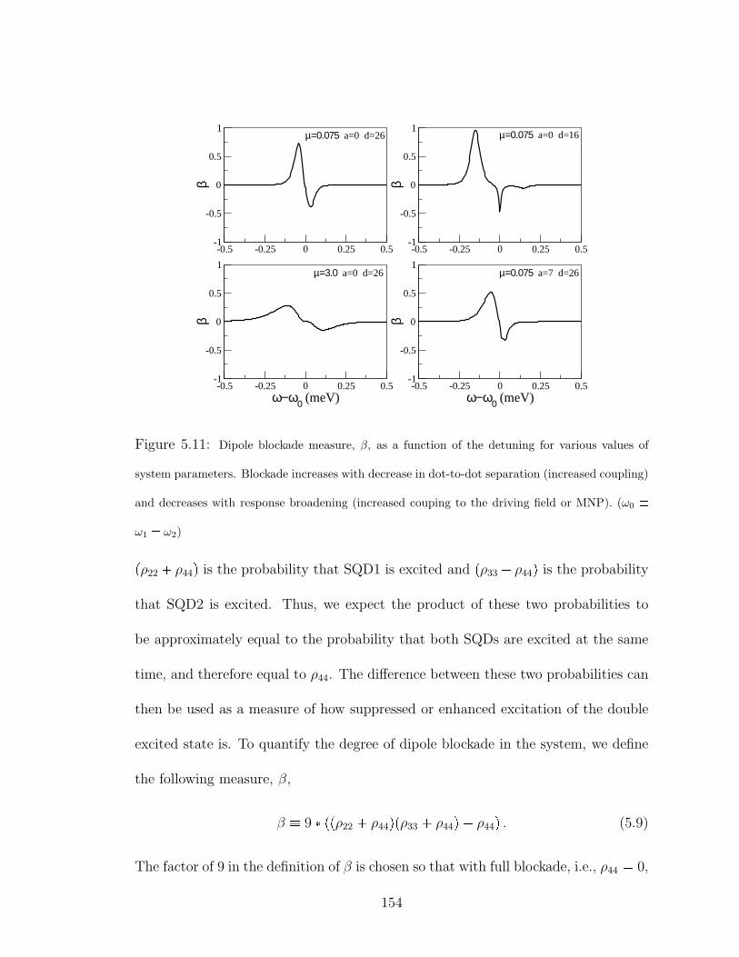
-0.5 -0.25 0 0.25 0.5-1
-0.5
0
0.5
1
β
-0.5 -0.25 0 0.25 0.5-1
-0.5
0
0.5
1
β-0.5 -0.25 0 0.25 0.5
ω−ω0 (meV)
-1
-0.5
0
0.5
1
β
-0.5 -0.25 0 0.25 0.5ω−ω0 (meV)
-1
-0.5
0
0.5
1
β
µ=0.075 a=0 d=26 µ=0.075 a=0 d=16
µ=0.075 a=7 d=26µ=3.0 a=0 d=26
Figure 5.11: Dipole blockade measure, β, as a function of the detuning for various values of
system parameters. Blockade increases with decrease in dot-to-dot separation (increased coupling)
and decreases with response broadening (increased couping to the driving field or MNP). (ω0 ω1 ω2)pρ22 ρ44q is the probability that SQD1 is excited and pρ33 ρ44q is the probabilitythat SQD2 is excited. Thus, we expect the product of these two probabilities to
be approximately equal to the probability that both SQDs are excited at the same
time, and therefore equal to ρ44. The difference between these two probabilities can
then be used as a measure of how suppressed or enhanced excitation of the double
excited state is. To quantify the degree of dipole blockade in the system, we define
the following measure, β,
β 9 ppρ22 ρ44qpρ33 ρ44q ρ44q . (5.9)
The factor of 9 in the definition of β is chosen so that with full blockade, i.e., ρ44 0,
154
at saturation (ρ11 ρ22 ρ33 13), β 1. This is essentially the maximum value
of β in the steady state limit (without population inversion). Conversely, if the
interaction between the dots is strong enough, then their resonances will be shifted
with respect to their bare resonances. In such a case, with the driving field near the
bare SQD resonance, the excitation of a single SQD, ρ22 and ρ33, will be suppressed
relative to ρ44 and β 0. In the actual calculations performed, values of β 0.5were rare.
When we plot β for various values of the system parameters, we find that
blockade increases when the SQD-SQD separation is decreased as expected (see
Figure 5.11). The stronger coupling between the dots increases the splitting between
the two levels. For a detuning near the symmetric mode resonance, that mode is
much more likely to be filled than the antisymmetric state, which is at a much
higher energy. Thus double excitation of the dots is suppressed. When coupling to
the driving field is increased (by increasing µ) or coupling to the MNP is increased
(by increasing a), the SQD response broadens, providing more overlap between the
two single exciton states and thus decreasing the dipole blockade.
5.4.4 Comparison in the Weak SQD-SQD Coupling Regime
When there is strong SQD-SQD coupling, the semiclassical and quantum ap-
proaches produce very different results. However, when the direct coupling between
the SQDs is weaker, the detuning of the symmetric and antisymmetric states is
smaller. Furthermore, in the presence of an MNP, the coupling mediated by the
155
plasmons can become more significant than the direct coupling between the SQDs.
It is then expected that two approaches would be more in agreement in this regime.
In Figure 5.12, we plot the results of the two models in the regime with weak
SQD-SQD coupling (µ1 µ2 0.5 enm), and strong SQD-MNP coupling (a 7 nm, R1 R2 13 nm). Shown for each model are the diagonal density matrix
elements of the symmetric/antisymmetric basis (ρ11, ρSS, ρAA, ρ44) and the blockade
measure, β. Also shown are the real and imaginary parts of the transition dipole mo-
ment of the symmetric state, µSS, which we calculate as µSS ρ1S ρS1 ρS4 ρ4S.
When the two models are compared (top vs bottom of Figure 5.12), we see
similarities between the semiclassical and quantum models in the general shape of
the predicted responses. However, there is significant deviation between the two
models as well. In particular, the semiclassical approach does not account for the
dipole blockade that occurs in the quantum model. Even with weak SQD-SQD
coupling, dipole blockade can still have a significant impact on system behavior.
This leads to noted differences between the two models in the regions just above
and below the SQD bare resonance, where β reaches extreme values.
In the quantum model, the differences highlighted in Figure 5.12 are most
notable in the slight splitting shown in ρ11, very sharp peak of ρ44 and the enhance-
ment in ρSS that occurs just below the SQD bare resonance. These effects are due to
dipole blockade. In the case of ρSS, this enhancement is just the location of the sym-
metric eigenstate. Interestingly, ρAA is also peaked at this same energy and appears
to be identical to ρSS. However, the reason that ρSS ρAA in the steady state limit
is simply due to mixing between the symmetric and antisymmetric modes from the
156
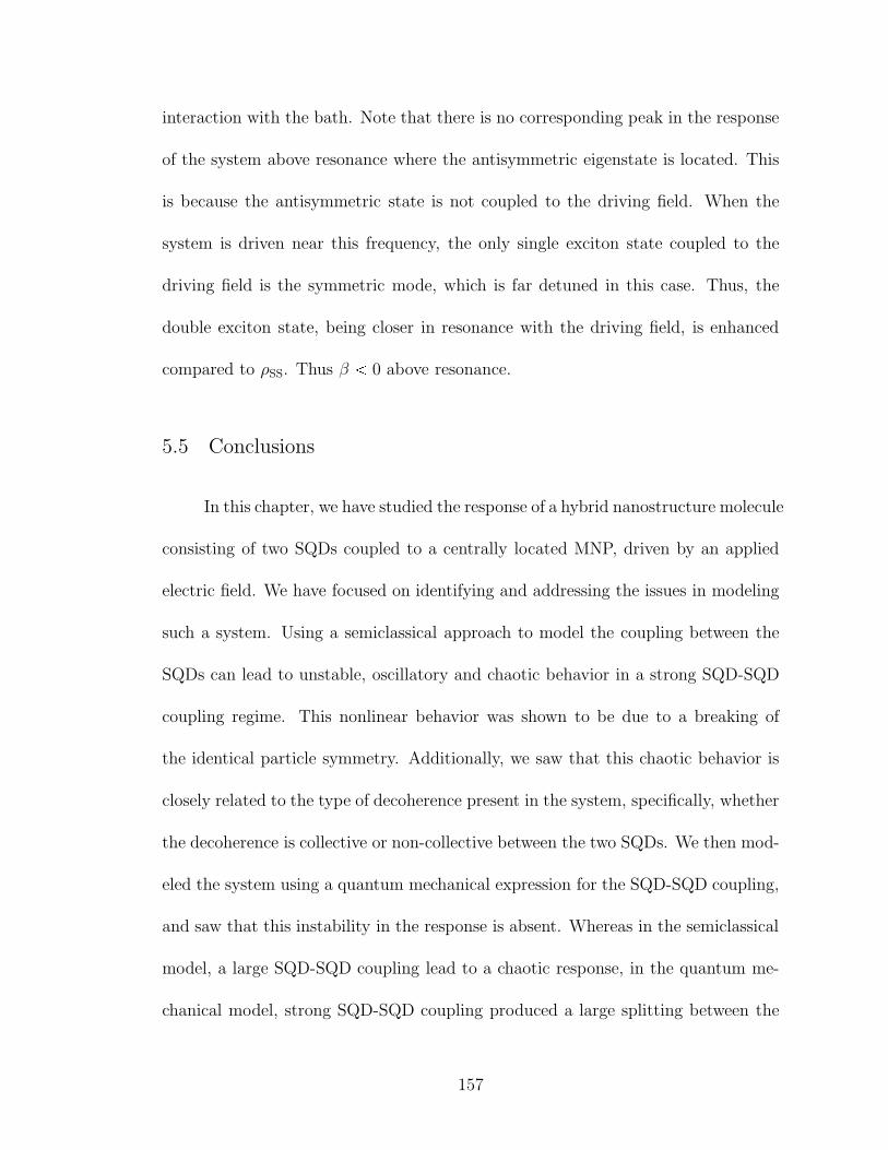
interaction with the bath. Note that there is no corresponding peak in the response
of the system above resonance where the antisymmetric eigenstate is located. This
is because the antisymmetric state is not coupled to the driving field. When the
system is driven near this frequency, the only single exciton state coupled to the
driving field is the symmetric mode, which is far detuned in this case. Thus, the
double exciton state, being closer in resonance with the driving field, is enhanced
compared to ρSS. Thus β 0 above resonance.
5.5 Conclusions
In this chapter, we have studied the response of a hybrid nanostructure molecule
consisting of two SQDs coupled to a centrally located MNP, driven by an applied
electric field. We have focused on identifying and addressing the issues in modeling
such a system. Using a semiclassical approach to model the coupling between the
SQDs can lead to unstable, oscillatory and chaotic behavior in a strong SQD-SQD
coupling regime. This nonlinear behavior was shown to be due to a breaking of
the identical particle symmetry. Additionally, we saw that this chaotic behavior is
closely related to the type of decoherence present in the system, specifically, whether
the decoherence is collective or non-collective between the two SQDs. We then mod-
eled the system using a quantum mechanical expression for the SQD-SQD coupling,
and saw that this instability in the response is absent. Whereas in the semiclassical
model, a large SQD-SQD coupling lead to a chaotic response, in the quantum me-
chanical model, strong SQD-SQD coupling produced a large splitting between the
157
0
1
ρ 11
0
0.5
ρ SS
-0.3
0.3
µ SS
-0.2 -0.1 0 0.1 0.20
0.5
ρ 44
-0.2 -0.1 0 0.1 0.2ω − ω0 (meV)
0
0.5
ρ AA
-0.2 -0.1 0 0.1 0.2-1
1
β
0
1
ρ 11
0
0.5
ρ SS
-0.3
0.3µ SS
-0.2 -0.1 0 0.1 0.20
0.5
ρ 44
-0.2 -0.1 0 0.1 0.2ω − ω0 (meV)
0
0.5
ρ AA
-0.2 -0.1 0 0.1 0.2-1
1
β
Sem
i-C
lass
ical
Qua
ntum
a = 7 nm µ1 = µ2 = 0.5 e nm
Figure 5.12: Comparison of semiclassical model (top 6 plots) and quantum model (bottom
6 plots) in the regime with weak SQD-SQD coupling (µ1 µ2 0.5 enm), and strong SQD-
MNP coupling (a 7 nm, R1 R2 13nm). Shown are the diagonal density matrix elements
(ρ11, ρSS, ρAA, ρ44) and the blockade measure, β. Also shown are the real (solid line) and imaginary
(dotted line) parts of the transition dipole moment of the symmetric state, µSS ρ1SρS1ρS4ρ4S.
158
two single exciton states. We then compared the two models on a system with a
strong plasmon mediated interaction between the SQDs and a weak direct interac-
tion between them. In this case, we found that while the results of the two models
were similar, dipole blockade and the level splitting of the single exciton states in
the quantum model are non-trivial effects even in this regime.
159

Chapter 6
Concluding Remarks
In this thesis, we have studied hybrid systems consisting of SQDs and MNPs.
Coupling the sharp, discrete resonance of the SQD to the broad continuum of plas-
monic modes supported by the MNP with an applied driving field near the exciton
resonance, should provide for dramatic signatures in the system response. We have
developed theory to identify these signatures. Furthermore, the ability of MNPs
to perform subwavelength confinement of light (in the form of plasmons), MNPs
are a promising candidate to facilitate the directed transport of excitations and/or
quantum information transfer between adjacent SQDs (or other types of quantum
emitters). Our results address the physics that underlies this paradigm.
To exploit this paradigm for quantum, nanoscale transport and communica-
tion, one needs to understand how MNPs act as nanoantennas and nanoguides.
One must understand the coupling between the exciton of the SQD and plasmons
in the MNP. One must also understand how SQD-to-SQD quantum communication
is modified by transfer via plasmons. Finally, one must understand how transfer
is further modified if the metal nanoparticles are small and quantum effects can
influence their response. In this thesis we have focused primarily on the effects of
coupling between the SQDs and the MNPs.
Realization of nanostructures composed of SQDs and MNPs for use in nanode-
160
vices will require accurate theoretical models, which can predict the hybrid system
response. Once these models are built, one can then use them to understand how the
coupling introduced between these nano-objects, alters and modifies the behavior of
each. By examining the conditions which cause different phenomena to emerge, one
could then predict regions of parameter space which best exhibit novel properties of
interest.
In this work, we have investigated the modification to the optical response
of SQD-MNP and SQD-MNP-SQD hybrid systems. In particular, we probed the
parameter space of these systems and identified a rich spectrum of phenomena: the
nonlinear Fano effect, exciton induced transparency, suppressed SQD response, and
bistability. We then located the regions of parameter space that lead to these distinct
regimes of system behavior and set bounds on each. By considering the regions of
parameter space where these phenomena occur, we were then able to deduce what
causes them to emerge.
We showed how constructive and destructive interference of the local fields,
internal to the system, with the external fields driving the hybrid structure is central
in determining the system response. Using this knowledge, we then looked at how we
could generalize these results to similar systems and more complicated structures.
We then saw that this knowledge could be exploited to engineer hybrid systems,
by tuning the SQD size and resonance, as well as the MNP geometry, to enhance
or to bias the system response towards a particular, desired behavior. Specifically,
we found that local field enhancement from nanorods can provide easier access to
strong SQD-MNP coupling regimes.
161
The effect of MNP size, shape and SQD placement was analyzed to determine
the regimes where the local multipolar response becomes significant. We identified
regimes where dark modes and higher order multipolar modes could influence hybrid
response. Strong, local field coupling via dark modes changes the interference and
self-interaction effects dramatically. External fields do not directly drive this MNP
dark mode, so SQD-MNP coupling is dominated by the local induced self-coupling.
Coupling to higher order modes could be critical for long-range excitation transfer
between different SQDs coupled to a nanorod.
To build realistic models that could allow for the simulation of hybrid nanos-
tructures, we employed many techniques. We examined a number of different ap-
proximation techniques, and discussed the assumptions and implications of each.
Furthermore, we employed these approximations in various coupling regimes and
compared the results against models which utilize differing methods. Such checks of
consistency allowed us to test the validity of our models in various limits. In partic-
ular, we saw that while a dipole approximation was sufficient to model the response
of a spherical MNP with a radius that is small compared to interparticle separation,
for larger spherical MNPs or elongated nanorods or wires, a more complete approach
was needed. This consideration led us to use a full electrodynamical calculation, us-
ing the boundary element method to determine the local induced field produced by
a nanorod. In the SQD-MNP-SQD system, we identified further issues in modeling
such a system. Specifically, we saw that modeling the coupling between the SQDs
semiclassically could lead to unstable and oscillatory behavior in the steady state.
This chaotic behavior which arises in the semiclassical model, required a quantum
162
mechanical model to properly account for the coupling between the SQDs.
6.1 Looking Ahead
Work is now in progress to improve upon the models developed in this thesis.
Specifically, the exact quantum nature of the SQD-MNP interaction is being ex-
plored by treating the plasmon quantum mechanically. Such quantum mechanical
corrections to the semiclassical SQD-MNP model would become important for a
number of reasons. For one, very small metallic structures will begin to confine the
plasmons. Recently, it has been shown that even MNPs as large as 10 nm in diam-
eter will begin to exhibit plasmon resonances which diverge from values predicted
classically due to a change in particle permittivity in the quantum regime [66]. Fur-
ther reducing the MNP size will eventually lead to the appearance of sharp, distinct
modes replacing the broad continuous response of larger MNPs [61, 62]. Perhaps
more importantly, a quantum mechanical treatment of the plasmons is necessary if
we wish to investigate corrections introduced by quantum mechanical coupling for
the SQD-MNP interaction. For example, the quantum nature of exciton-plasmon-
exciton conversion (for either transfer between SQDs or the self-interaction of an
SQD) determines the loss of quantum information that occurs in the process.
Recently, several theoretical investigations have gone beyond the semiclassical
limit in studying SQD/MNP hybrids by treating the plasmon-exciton interaction
with quantum mechanical methods, such as treating the plasmon in the quasi-mode
formalism commonly employed in cavity QED [58, 59], or by using Green’s function
163
techniques [67]. In the quasi-mode method, the plasmon is modeled as a single,
broad, effective mode which couples to the exciton. This mode is then often traced
out of the problem by invoking the very fast nature of the plasmon relaxation (com-
pared to the relatively long lived exciton). However, in certain situations, this large
hierarchy of time scales might not hold. In fact, since metallic nanostructures can
have large Purcell factors, close proximity of the SQD can greatly enhance the emis-
sion rate of the exciton, by as much as a few orders of magnitude or more. This
can reduce the range of time scales of the system interactions, and could lead to a
more coherent coupling between SQD and MNP. Such a system would provide for
fast excitation transfer, and a reduction in the loss of quantum information.
Currently, work is being done to build more advanced models to more accu-
rately predict SQD-MNP and SQD-MNP-SQD hybrid behavior in the case where
the quantum nature of the coupling is important. These models treat the plasmons
in a quantum mechanical manner with a quasi-mode approach. Rather than trace
over the plasmon mode, which assumes a non-coherent exciton-plasmon coupling,
we retain the plasmon mode in the problem and determine the evolution of both
the exciton and plasmon states. The evolution of the system is calculated using
a quantum trajectory method [68], in which a system’s evolution is governed by a
non-Hermitian, effective Hamiltonian, and spontaneous decay is simulated by Monte
Carlo-determined “quantum jumps”. By treating the exciton-plasmon coupling fully
quantum mechanical, one should be able to answer questions that necessitate a co-
herent exciton-plasmon coupling. The work presented in this thesis has been an
integral component in the building of these models.
164
Bibliography
[1] R. P. Feynman. There’s plenty of room at the bottom. Eng. Sci., 23:22–36,1960.
[2] G. Binnig, H. Rohrer, Ch. Gerber, and E. Weibel. Surface studies by scanningtunneling microscopy. Phys. Rev. Lett., 49:57–61, Jul 1982.
[3] Eigler D. M. and Schweizer E. K. Positioning single atoms with a scanningtunneling microscope. Nature, 344:524–526, 1990.
[4] H. W. Kroto, J. R. Heath, S. C. O’Brien, R. F. Curl, and R. E. Smalley. C$ 60$:Buckminsterfullerene. Nature, 318(6042):162–163, November 1985.
[5] HW Kroto. The stability of the fullerenes cn, with n= 24, 28, 32, 36, 50, 60and 70. Nature, 329(6139):529–531, 1987.
[6] Sumio Iijima. Helical microtubules of graphitic carbon. Nature, 354(6348):56–58, November 1991.
[7] W.K. Leutwyler, S.L. Burgi, and HB Burgl. Semiconductor clusters, nanocrys-tals, and quantum dots. Science, 271:933, 1996.
[8] L. Banyai and S.W. Koch. Semiconductor quantum dots, volume 2. WorldScientific Publishing Company Incorporated, 1993.
[9] D.L. Fedlheim and C.A. Foss. Metal nanoparticles: synthesis, characterization,
and applications. CRC, 2001.
[10] K.L. Kelly, E. Coronado, L.L. Zhao, and G.C. Schatz. The optical propertiesof metal nanoparticles: the influence of size, shape, and dielectric environment.The Journal of Physical Chemistry B, 107(3):668–677, 2003.
[11] S.H. Yu, M. Antonietti, H. Colfen, and J. Hartmann. Growth and self-assemblyof bacro4 and baso4 nanofibers toward hierarchical and repetitive superstruc-tures by polymer-controlled mineralization reactions. Nano Letters, 3(3):379–382, 2003.
[12] J. Barauskas, M. Johnsson, and F. Tiberg. Self-assembled lipid superstructures:beyond vesicles and liposomes. Nano letters, 5(8):1615–1619, 2005.
[13] J. Lee, A.O. Govorov, and N.A. Kotov. Bioconjugated superstructures of cdtenanowires and nanoparticles: Multistep cascade forster resonance energy trans-fer and energy channeling. Nano letters, 5(10):2063–2069, 2005.
[14] Christian Gruber, Primoz Kusar, Andreas Hohenau, and Joachim R. Krenn.Controlled addressing of quantum dots by nanowire plasmons. Applied Physics
Letters, 100(23):231102, 2012.
165

[15] T. Pons, I.L. Medintz, K.E. Sapsford, S. Higashiya, A.F. Grimes, D.S. English,and H. Mattoussi. On the quenching of semiconductor quantum dot photolu-minescence by proximal gold nanoparticles. Nano Lett., 7(10):3157–3164, 2007.
[16] A.V. Akimov, A. Mukherjee, C.L. Yu, D.E. Chang, A.S. Zibrov, P.R. Hemmer,H. Park, and M.D. Lukin. Generation of single optical plasmons in metallicnanowires coupled to quantum dots. Nature, 450(7168):402–406, 2007.
[17] Y. Fedutik, V. V. Temnov, O. Schops, U. Woggon, and M. V. Artemyev.Exciton-plasmon-photon conversion in plasmonic nanostructures. Phys. Rev.
Lett., 99(13):136802, 2007.
[18] H. Mertens, J.S. Biteen, H.A. Atwater, and A. Polman. Polarization-selectiveplasmon-enhanced silicon quantum-dot luminescence. Nano Lett., 6(11):2622–2625, 2006.
[19] Alberto G. Curto, Giorgio Volpe, Tim H. Taminiau, Mark P. Kreuzer, RomainQuidant, and Niek F. van Hulst. Unidirectional emission of a quantum dotcoupled to a nanoantenna. Science, 329(5994):930–933, 2010.
[20] Wei Zhang, Alexander O. Govorov, and Garnett W. Bryant. Semiconductor-metal nanoparticle molecules: Hybrid excitons and the nonlinear fano effect.Phys. Rev. Lett., 97(14):146804, 2006.
[21] Ryan D. Artuso and Garnett W. Bryant. Optical response of strongly coupledquantum dotmetal nanoparticle systems: Double peaked fano structure andbistability. Nano Lett., 8(7):2106–2111, June 2008.
[22] Ryan D. Artuso and Garnett W. Bryant. Strongly coupled quantum dot-metal nanoparticle systems: Exciton-induced transparency, discontinuous re-sponse, and suppression as driven quantum oscillator effects. Phys. Rev. B,82(19):195419, Nov 2010.
[23] Jie-Yun Yan, Wei Zhang, Suqing Duan, Xian-Geng Zhao, and Alexander O.Govorov. Optical properties of coupled metal-semiconductor and metal-molecule nanocrystal complexes: Role of multipole effects. Phys. Rev. B,77(16):165301, Apr 2008.
[24] SM Sadeghi. Tunable nanoswitches based on nanoparticle meta-molecules.Nanotechnology, 21:355501, 2010.
[25] A. Govorov, G. Bryant, W. Zhang, T. Skeini, J. Lee, N. Kotov, J. Slocik, andR. Naik. Exciton-plasmon interaction and hybrid excitons in semiconductor-metal nanoparticle assemblies. Nano Lett., 6(5):984–994, 2006.
[26] Mu-Tian Cheng, Shao-Ding Liu, Hui-Jun Zhou, Zhong-Hua Hao, and Qu-QuanWang. Coherent exciton-plasmon interaction in the hybrid semiconductor quan-tum dot and metal nanoparticle complex. Opt. Lett., 32(15):2125–2127, 2007.
166
[27] R. Esteban, T. V. Teperik, and J. J. Greffet. Optical patch antennas forsingle photon emission using surface plasmon resonances. Phys. Rev. Lett.,104(2):026802, Jan 2010.
[28] J. Lindberg, K. Lindfors, T. Setala, and M. Kaivola. Dipole-dipole interactionbetween molecules mediated by a chain of silver nanoparticles. J. Opt. Soc.
Am. A, 24(11):3427–3431, 2007.
[29] S M Sadeghi, L Deng, X Li, and W-P Huang. Plasmonic (thermal) electromag-netically induced transparency in metallic nanoparticle–quantum dot hybridsystems. Nanotechnology, 20(36):365401, 2009.
[30] M. Liu, T.W. Lee, S.K. Gray, P. Guyot-Sionnest, and M. Pelton. Excitation ofdark plasmons in metal nanoparticles by a localized emitter. Phys. Rev. Lett.,102(10):107401, 2009.
[31] Mark L. Brongersma, John W. Hartman, and Harry A. Atwater. Electro-magnetic energy transfer and switching in nanoparticle chain arrays below thediffraction limit. Phys. Rev. B, 62(24):R16356–R16359, Dec 2000.
[32] D. E. Chang, A. S. Sørensen, P. R. Hemmer, and M. D. Lukin. Quantum opticswith surface plasmons. Phys. Rev. Lett., 97(5):053002, Aug 2006.
[33] A. Gonzalez-Tudela, D. Martin-Cano, E. Moreno, L. Martin-Moreno, C. Teje-dor, and F. J. Garcia-Vidal. Entanglement of two qubits mediated by one-dimensional plasmonic waveguides. Phys. Rev. Lett., 106:020501, Jan 2011.
[34] E. Altewischer, M. P. van Exter, and J. P. Woerdman. Plasmon-assisted trans-mission of entangled photons. Nature, 418(6895):304–306, 2002.
[35] Sylvain Fasel, Franck Robin, Esteban Moreno, Daniel Erni, Nicolas Gisin, andHugo Zbinden. Energy-time entanglement preservation in plasmon-assistedlight transmission. Phys. Rev. Lett., 94(11):110–501, 2005.
[36] Giuliana Di Martino, Yannick Sonnefraud, Stephane Kena-Cohen, Mark Tame,Sahin K. Ozdemir, M. S. Kim, and Stefan A. Maier. Quantum statisticsof surface plasmon polaritons in metallic stripe waveguides. Nano Letters,12(5):2504–2508, 2012.
[37] Oriane Mollet, Serge Huant, Geraldine Dantelle, Thierry Gacoin, and AurelienDrezet. Quantum plasmonics: Second-order coherence of surface plasmonslaunched by quantum emitters into a metallic film. Phys. Rev. B, 86:045401,Jul 2012.
[38] Ryan D. Artuso, Garnett W. Bryant, Aitzol Garcia-Etxarri, and Javier Aizpu-rua. Using local fields to tailor hybrid quantum-dot/metal nanoparticle systems.Phys. Rev. B, 83:235406, Jun 2011.
167
[39] Michael Faraday. The bakerian lecture: Experimental relations of gold (andother metals) to light. Philosophical Transactions of the Royal Society of Lon-
don, 147:145–181, 1857.
[40] Gustav Mie. Beitrage zur optik truber medien, speziell kolloidaler met-allosungen. Annalen der Physik, 330(3):377–445, 1908.
[41] L. Rayleigh. On the scattering of light by small particles. Philosophical Maga-
zine, 41(275):447–451, 1871.
[42] R. H. Ritchie. Plasma losses by fast electrons in thin films. Physical Review,106:874–881, June 1957.
[43] J.D. Jackson and R.F. Fox. Classical electrodynamics. American Journal of
Physics, 67:841, 1999.
[44] Matthew Pelton and Garnett W. Bryant. Introduction to Metal-Nanoparticle
Plasmonics. John Wiley and Sons, New York, 2013.
[45] F. Assous, P. Degond, E. Heintze, P.A. Raviart, and J. Segre. On a finite-element method for solving the three-dimensional maxwell equations. Journal
of Computational Physics, 109(2):222 – 237, 1993.
[46] G. Mur. Absorbing boundary conditions for the finite-difference approximationof the time-domain electromagnetic-field equation. IEEE Trans. Electromag.
Compat., 23(4):377–382, 1981.
[47] F. J. Garcia de Abajo and A. Howie. Relativistic electron energy loss andelectron-induced photon emission in inhomogeneous dielectrics. Phys. Rev.
Lett., 80:5180–5183, Jun 1998.
[48] A. Yariv. Quantum Electronics. John Wiley and Sons, New York, 1975.
[49] C. Gardiner and P. Zoller. Quantum Noise. Springer-Verlag, Berlin Heidelberg,2004.
[50] G. Lindblad. On the generators of quantum dynamical semigroups. Commu-
nications in Mathematical Physics, 48:119–130, 1976. 10.1007/BF01608499.
[51] A. Kossakowski. On quantum statistical mechanics of non-hamiltonian systems.Reports on Mathematical Physics, 3(4):247 – 274, 1972.
[52] Hongxing Xu, Xue-Hua Wang, Martin P. Persson, H. Q. Xu, Mikael Kall,and Peter Johansson. Unified treatment of fluorescence and raman scatteringprocesses near metal surfaces. Phys. Rev. Lett., 93(24):243002, Dec 2004.
[53] M Durach, A Rusina, V I Klimov, and M I Stockman. Nanoplasmonic renor-malization and enhancement of coulomb interactions. New Journal of Physics,10(10):105011, 2008.
168
[54] L.D. Landau, E.M. Lifshitz, and L.P. Pitaevskii. Electrodynamics of Continuous
Media. Butterworth-Heinemann Ltd, Oxford, 1984.
[55] P. B. Johnson and R. W. Christy. Optical constants of the noble metals. Phys.Rev. B, 6(12):4370–4379, Dec 1972.
[56] K. L. Silverman, R. P. Mirin, S. T. Cundiff, and A. G. Norman. Direct measure-ment of polarization resolved transition dipole moment in ingaas/gaas quantumdots. Applied Physics Letters, 82(25):4552–4554, 2003.
[57] T. H. Stievater, Xiaoqin Li, D. G. Steel, D. Gammon, D. S. Katzer, D. Park,C. Piermarocchi, and L. J. Sham. Rabi oscillations of excitons in single quantumdots. Phys. Rev. Lett., 87(13):133603, Sep 2001.
[58] A. Ridolfo, O. Di Stefano, N. Fina, R. Saija, and S. Savasta. Quantum plas-monics with quantum dot-metal nanoparticle molecules: Influence of the fanoeffect on photon statistics. Phys. Rev. Lett., 105:263601, Dec 2010.
[59] Edo Waks and Deepak Sridharan. Cavity qed treatment of interactions betweena metal nanoparticle and a dipole emitter. Phys. Rev. A, 82:043845, Oct 2010.
[60] David Dzsotjan, Anders S. Sørensen, and Michael Fleischhauer. Quantum emit-ters coupled to surface plasmons of a nanowire: A green’s function approach.Phys. Rev. B, 82:075427, Aug 2010.
[61] E. Prodan and P. Nordlander. Exchange and correlations effects in small metal-lic nanoshells. Chemical Physics Letters, 349(12):153 – 160, 2001.
[62] Emily Townsend and Garnett W. Bryant. Plasmonic properties of metallicnanoparticles: The effects of size quantization. Nano Letters, 12(1):429–434,2012.
[63] Peng Song, Peter Nordlander, and Shiwu Gao. Quantum mechanical study ofthe coupling of plasmon excitations to atomic-scale electron transport. The
Journal of Chemical Physics, 134(7):074701, 2011.
[64] J. Forstner, C. Weber, J. Danckwerts, and A. Knorr. Phonon-assisted dampingof rabi oscillations in semiconductor quantum dots. Phys. Rev. Lett., 91:127401,Sep 2003.
[65] R. H. Lehmberg. Radiation from an n-atom system. i. general formalism. Phys.Rev. A, 2:883–888, Sep 1970.
[66] J.A. Scholl, A.L. Koh, and J.A. Dionne. Quantum plasmon resonances ofindividual metallic nanoparticles. Nature, 483(7390):421–427, 2012.
[67] A. Manjavacas, F. J. Garcia de Abajo, and P. Nordlander. Quantum plexciton-ics: Strongly interacting plasmons and excitons. Nano Letters, 11(6):2318–2323,2011.
169

[68] M. B. Plenio and P. L. Knight. The quantum-jump approach to dissipativedynamics in quantum optics. Rev. Mod. Phys., 70:101–144, Jan 1998.
170
Recommended