AC Losses Analysis in stack of 2G HTS tapes in a coil
V V Zubko1, S S Fetisov1, S Yu Zanegin1, V S Vysotsky1
1Russian Scientific R&D Cable Institute Moscow, Russia, 111024
E-mail: [email protected]
Abstract. The model coil with the racetrack geometry based on second generation (2G) High
Temperature Superconducting (HTS) tapes has been developed for an electrical machine where
a winding pack is a stack of 2G HTS tapes. It is important to evaluate transport current AC losses
and possible methods to reduce them in a winding. In a device made of 2G HTS tapes, the main
the AC losses are the hysteresis ones. Only numerical simulation permits to predict them in full.
The FEM model for calculation of the hysteresis losses developed before for 2G HTS power
cables was modified for a stack of the 2G HTS tapes in a coil. In this paper the methods to
increase a computational speed are presented. Possible ways to reduce AC losses are discussed
also. The details of the model and comparisons of calculations with measurements of the AC
loss are presented.
1. Introduction
Application of the HTS conductors in the coils of complex HTS devices, for example, of electrical
machines, increases efficiency due to considerably higher current density and decreases mass and overall
dimensions. Various AC, DC device architectures based on this advantage, have been evaluated.
Review of the current situation of numerical modelling in the context of HTS device development is
presented in [1, 2]. Numerical modeling is a key component towards optimization of HTS devices, and
it is a field in development, especially regarding electromagnetic models.
In case of the cyclic variations of transport current one of the major tasks in the HTS devices design
is a minimization of transport current AC losses. In terms of very complex objects only numerical
calculation can provide AC loss prediction.
A lot of advanced models for computing of the losses in HTS tapes, wires and devices are developed
in recent years, the review of the numerical modeling is presented in [3]. Most of the situations relevant
to realistic applications can be modeled in 2-D but the most challenging step for the scientific community
is a transition to 3-D calculations. For example, simulation of losses in stacks of the HTS tapes can be
based on the following models: finite element methods (FEM) [4-6], variational formulation [7-9].
The full consideration and computer simulation of the AC losses in 2G HTS stacks has its own
characteristics and represents a sophisticated task. The proper model should take into account the
following: high aspect ratio (width/thickness) of 2G HTS layer in the tape; strong nonlinearity between
resistivity and current density of the HTS materials; the losses in a thin superconducting layer depending
on transport current and corresponding magnetic field magnitude and orientation; the non-uniformity of
critical current density across the width of a tape (critical current density on the edges of the tape may
be less than in its middle at zero magnetic field); hysteretic behavior of the magnetic substrate; the
substrate ferromagnetism depending on magnetic field magnitude.
In this paper the AC losses in HTS coil winding is studied numerically and experimentally verified,
all factors are taken into account to develop the FEM model for proper calculations of AC losses in the
2G HTS tape coil.
2. Model to analyse AC losses
The FEM model for calculation of AC losses using the finite-element ANSYS code [10] had been
developed before for 2G HTS power cables [11]. In this work it was modified for stack of 2G HTS tapes
in the coil.
The AC losses in a HTS coil consist of: hysteresis losses, caused by the penetration of the magnetic
flux in the superconducting material, hysteresis losses in magnetic materials, eddy current losses in the
normal metal parts of a HTS coil. Thus, the transient electromagnetic analysis is necessary to simulate
the AC losses. The developed FEM model uses ANSYS with help of APDL (ANSYS Parametric Design
Language) - an efficient method for engineering simulation of the 3D and 2D transient electromagnetic
analysis in the devices. For these cases ANSYS implements the magnetic vector potential formulation
which uses three degree of freedom in the non-conducting regions, the magnetic vector potential
components, and adds an extra degree of freedom: the time-integrated electric voltage in the conducting
regions (A,V-A formulation). ANSYS can calculate eddy current distribution in any conventional
conductors without taking into account the nonlinear resistivity. Also ANSYS is able to solve processes
for real nonlinear anisotropic magnetic materials, as there is a capability for modelling B-H curves and
therefore, the hysteresis losses in the magnetic materials can be calculated. For example, we used 3D
model for the calculation of hysteresis losses in a NiW substrate of the 2G HTS tapes of the power cable
[12].
To simulate hysteresis losses in the 2G HTS layer of the tape its strong nonlinear resistivity must be
taken into account. Mainly due to high aspect ratio of 2G HTS layer in the tape (large number of small
elements in the complete mesh) and the nonlinear resistivity of the HTS materials (a large number of
iterations are required), a simulation of the hysteresis losses in the superconducting material is the most
difficult task and requires long calculation time and demands large computer memory. 2-D models must
be used for drastically reduction of time and complexity of calculation of the hysteresis losses.
Power law relation is usually used to express the nonlinearity between resistivity (ρ) and current
density (J) of the superconductor:
1
0, ,
, ,
n
c c
E JJ B x
J B x J B x
, (1)
where E0 = 1μV/cm is the electric field, when the critical current density is reached, and n is a power
law index. We used equation from paper [13] to determine the critical current density dependence on
magnetic field ( )cJ B
. We also used a standard piecewise linear function Jc0(x) (like in paper [3]) to
describe the non-uniformity of critical current density at zero magnetic field across a HTS layer. So for
the critical current density in the HTS layers the following expression was used:
0
0
0.52 2 2
0
, , , ,
1 cos ( ) sin ( )
c
c c c c
J xJ B x J B x J B J x
Bk
B
, (2)
where θ is an orientation angle of magnetic field with respect to the tape normal, k, B0 and β are the
parameters used here for the Jc(B,θ) fitting, α - accounts the fact that critical current of the tape (Ic) is
derived from measurements with the self-field of the tape.
Function Jc0(x) is symmetric about centre of the tape and is defined by equation:

0 0
1, , / 2
2 11 , , / 2
1
w
c c c JJ w
w
if x h w
J x J x hh if x h w
w h
, (3)
where 0 < hJ < 1, 0 < hw < 1 are input parameters, Jc0c - critical current density from the centre across
the HTS layer up to hw∙w/2. For the case if only Ic of the tape was measured and thus the Jc0c can be
calculated from equation0
0(x)dx
wc
chts
IJ
, where w and δhts are the width and the thickness of the
HTS layer.
For realization of the possibility to calculate losses, the FEM model using ANSYS needs to include
the above dependencies. These can be realized by iteration algorithm, which is based on the fact that the
field penetration into the superconductor can be always simulated by solving eddy current distribution
in a conventional conductor divided into elements that have local resistivity [4].
First a FEM model in ANSYS has to be built and the initial value of resistivity for each (i) element
of HTS layer (ρ0i) has to be set. Further, we can compute the currents density (Ji) in the element. Then
(1) the resistivity is iteratively changed according to power low relation:
1
0 1 0
, ,
, ( )
nk
k k ii i i
c i c i
E Jf
J J
. (4)
Stopping criterion for the resistivity of each element is
1k k
i i
k
i
.
For 2G HTS layers the appropriate minimum initial values of ρ0i are 10-17 Ω·m and ζ is 10-4.
While using power low relation (4) the resistivity at k+1-th iteration ρk+1i it is better to calculate the
equation with the relaxation factor α = 0.1:
1 1k k k k
i i i i . (5)
To solve the equations in form ρ = f(ρ), we have to use iterative procedure, which is known as the
method of successive substitution.
After all iterations hysteresis losses in the HTS layer per unit length and per cycle are given by:
1
1
4N N
i i
i i
Q J . (6)
Where N- number of mesh elements in the HTS layer, N1 - number of step in time-dependent solution
from 0 to maximal value of the applied transport current Im (1/4 total cycle), Δτ - time step.
For engineering simulation of losses the further increase of the computational speed of the FEM
model is needed, so the following standard optimization methods were used:
1. ‘‘Bean model’’ assumption, where for n in iteration process, the following function for
the resistivity at k+1-th iteration for each (i) mesh element can be used:
1
,
kk k ii i
c i
J
J (7)
2. For acceleration of convergence equations in form ρ = f(ρ) the Wegstein method is suitable, and
it was implemented into our FEM model:

0 1 0
1 1
1
1 1
, ( )
( ) ( ) ( ( ) )( ) , 2
( ) ( ) ( )
i i i
k k k k
i i i ik k
i i k k k k
i i i i
f
f f ff k
f f
(8)
In addition to acceleration of convergence, the Wegstein method converges even under conditions
when the method of successive substitution does not.
3. Because that AC losses in HTS layers are hysteresis losses, it means they do not depend on
frequency. The losses are uniquely determined by the current density profiles in the HTS layers at the
maximal magnitude of the applied current. Losses independence from frequency makes it possible to
make only one step in time-dependent solution at Im. This means that Δτ = 1/4 total cycle. And we can
use vector potential approach for calculation of the hysteresis losses. A crucial ingredient of the vector
potential method is the existence of an electric center (kernel) [14], i.e. a region or line inside the
superconductor in which the electric field stays zero throughout the ac cycle. And losses in the HTS
layer per unit length and per cycle are given by from equation:
, ,04N
i z i z i
i
Q J A A s , (9)
where Az,i is the magnetic vector potential at a node of each (i) mesh elements, Az is the magnetic
vector potential at a node near the kernel.
Using the methods 1-3, the maximum number of iterations are about 5-40 to convergence (ζ is 10-4)
to calculate the AC losses at the applied transport current.
3. The test facility
An experimental technique has been developed and implemented to measure AC losses by direct
electrical method in the HTS coil [15]. The special test bench for detailed measurements of losses in
each tape of the linear part of the HTS coil winding of electric machine was developed. It represents
several HTS tapes placed in a stack or several stacks of tapes. The electrical scheme of AC losses
measurements is shown on figure 1.
Tapes from 1 to Nt (number depends on the experiment) with 200 mm distance between potential
taps are connected in parallel, insulated from each other with polyester film tape and contracted in a
stack. On the other hand, the tapes should be connected in series, like in a real winding, but that
schematic assumes presence of long interconnections between ends of tapes, thus forming additional
AC interferences that degrade small-signal quality from potential taps. Balancing resistors
(Rb_1…Rb_n) with 2% tolerance of value and parasitic inductance are used to eliminate current
distribution effects. In figure 2 photo of spreaded ends of tapes with individual current leads is shown.
Programmable power supply (PS) is capable to drive current up to 4kA in the range from 17 Hz to
400 Hz. Signals from voltage taps and from precision current sensor are recorded by Data Acquisition
System with 1Ms/s rate. Electrical losses are determined by direct electrical method, where active power
is determined by formula:
0
1 mt
m
P u idtt
, (10)
where u, i – instantaneous values of current and voltage, tm – measurement time (several periods of
signal to improve accuracy).
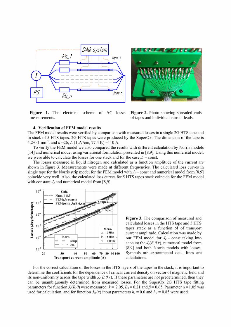
Figure 1. The electrical scheme of AC losses
measurements.
Figure 2. Photo showing spreaded ends
of tapes and individual current leads.
4. Verification of FEM model results
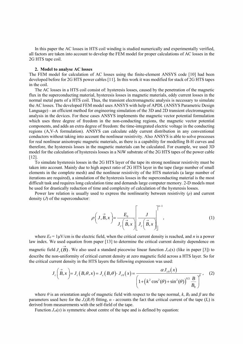
The FEM model results were verified by comparison with measured losses in a single 2G HTS tape and
in stack of 5 HTS tapes. 2G HTS tapes were produced by the SuperOx. The dimension of the tape is
4.2·0.1 mm2, and n ~26; Ic (1μV/cm, 77.4 K) ~110 A.
To verify the FEM model we also compared the results with different calculation by Norris models
[14] and numerical model using variational formulation presented in [8,9]. Using this numerical model,
we were able to calculate the losses for one stack and for the case Jc – const.
The losses measured in liquid nitrogen and calculated as a function amplitude of the current are
shown in figure 3. Measurements were made at different frequencies. The calculated loss curves in
single tape for the Norris strip model for the FEM model with Jc – const and numerical model from [8,9]
coincide very well. Also, the calculated loss curves for 5 HTS tapes stack coincide for the FEM model
with constant Jc and numerical model from [8,9].
Figure 3. The comparison of measured and
calculated losses in the HTS tape and 5 HTS
tapes stack as a function of of transport
current amplitude. Calculation was made by
our FEM model for Jc - const taking into
account the Jc(B,θ,x), numerical model from
[8,9] and both Norris models with losses.
Symbols are experimental data, lines are
calculations.
For the correct calculation of the losses in the HTS layers of the tapes in the stack, it is important to
determine the coefficients for the dependence of critical current density on vector of magnetic field and
its non-uniformity across the tape width Jc(B,θ,x). If these parameters are not predetermined, then they
can be unambiguously determined from measured losses. For the SuperOx 2G HTS tape fitting
parameters for function Jc(B,θ) were measured: k = 2.05, B0 = 0.21 and β = 0.65. Parameter α =1.05 was
used for calculation, and for function Jc0(x) input parameters hJ = 0.6 and hw = 0.85 were used.

From figure 3 one can see that the calculated losses curve coincide with experimental results, only if
dependence Jc(B,θ,x) is taken into account.
5. AC losses in stacks of 2G HTS tapes analysis
Stack of 15 2G HTS tapes and 3 stacks of 5 2G HTS tapes have been fabricated. 2G HTS tapes produced
also by the SuperOx with parameters: dimension - 3·0.1 mm2; n ~ 36; Ic (1μV/cm, 77.4 K) ~150 A.
Thickness of the tape insulation is 60 μm.
Measurements of losses were performed at different frequencies. There is no frequency dependence
of AC loss in the stacks which corresponds with the hysteresis nature of AC loss in all measurements.
In calculations of the losses the same parameters as in the section 4 for function Jc(B,θ) were used. For
function Jc0(x) input parameters hJ = 0.9 and hw = 0.85 were applied.
Figure 4 illustrates the measured and calculated losses. The losses per one tape and per meter in the
3 stacks of 5 tapes are shown as a function of the current amplitude. The same result is in figure 5 for
the 15 HTS tapes stack are shown. The measured current losses of the coil are in good agreement with
the computed data.
Figure 4. The comparison of losses measured and
calculated by the FEM model in the 3×5 HTS tapes
stacks as a function of the transport current
amplitude.
Figure 5. The comparison of losses measured
and calculated by the FEM model in the 15 HTS
tapes stack as a function of the transport current
amplitude.
Due to the implementation of the critical current density dependence on the vector magnetic field
and its non-uniformity across the tapes width Jc(B,θ,x) into our FEM model, the computed losses in the
stacks were in good agreement with the measured data.
The distribution of a total magnetic field for both models simulated at the moment when the peak
current equals 80 A, are shown in figure 6 and figure 7.
Figure 6. Magnetic field distribution in 3 stacks consisting of 5 tapes at the moment
when the instantaneous value of a transport current is 80A.

The distribution of a current density in the HTS layers of the stack consisting of 15 tapes, at the
moment when the peak current equals 80 A, are shown in figure 8.
Figure 7. Magnetic field distribution in the stack
consisting of 15 tapes at the moment when the
instantaneous value of a transport current is 80A.
Figure 8. The current density distribution in
the HTS layers of the stack consisting of 15
tapes at the moment when the instantaneous
value of a transport current is 80A.
6. AC losses in the HTS coils analysis
Two racetrack double pancake coils for electrical machine have been fabricated from 2G HTS tapes
produced by the SuperOx and AMSC [17] companies. In both coils the inner radius is 10 mm; the length
of straight part is 70 mm and total number of turns is 24.
6.1. The racetrack double pancake coil with the SuperOx tapes
SuperOx 2G HTS tape has had the following parameters: dimension without insulation 4.2·0.1 mm2 (the
insulation thickness is 15 μm); n ~ 30; Ic (1μV/cm, 77.4 K) ~ 150 A.
The AC losses per meter were calculated for two cross-sections of the racetrack coil: W1 - in the centre of the straight part in the Cartesian coordinate system and W2 in the centre of the coil end in the
cylindrical coordinate system with inner radius of the racetrack coil. The losses are Wcoil=L1·W1+L2·W2,
where L1 and L2 are lengths of tapes in the straight part and the coil end of the coil. For the function
Jc(B,θ) the same parameters were used in a calculation as in the section 4. For the function Jc0(x) the
input parameters hJ = 0.8 and hw = 0.85 were applied.
The measured and calculated by FEM model losses at three frequencies are compared in figure 9.
The measured current losses of the coil are in a good agreement with the computed data (Wcoil).
The distribution of a total magnetic field for two cross-sections of the racetrack coil simulated at the
moment when the peak current reaches 80 A, is shown in figure 10.
6.2. The racetrack double pancake coil with the AMSC tapes
AMSC 2G HTS tape has had the following parameters: dimensions without/with insulation are
4.8·0.21 mm2 and 4.95·0.36 mm2; n ~ 28; Ic (1μV/cm, 77.4 K) ~ 105 A. The AMSC 2G HTS tapes were
produced by the MOD/RABiTS™ process with use of NiW substrate that has a weak ferromagnetism.
The magnetism of the substrate affects the AC losses by two ways: the hysteresis behaviour of the
magnetic substrate generates hysteresis losses in the substrate itself; a high permeability of the substrate
can vary the magnetic field distribution around a HTS layer by increasing the magnetic field component
normal to it.
The AC losses per meter were also calculated for two cross-sections of the racetrack coil. In
calculation for this 2G HTS tape the following parameters for the function Jc(B,θ,x) were used: α = 1.02,
k=0.6, B0 = 0.45, β = 0.65, hJ = 1 and hw = 1.
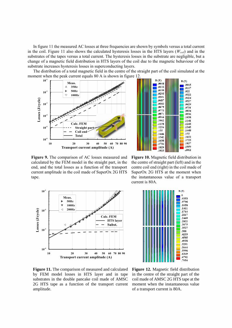
In figure 11 the measured AC losses at three frequencies are shown by symbols versus a total current
in the coil. Figure 11 also shows the calculated hysteresis losses in the HTS layers (Wcoil) and in the
substrates of the tapes versus a total current. The hysteresis losses in the substrate are negligible, but a
change of a magnetic field distribution in HTS layers of the coil due to the magnetic behaviour of the
substrate increases hysteresis losses in superconducting layers.
The distribution of a total magnetic field in the centre of the straight part of the coil simulated at the
moment when the peak current equals 80 A is shown in figure 12.
Figure 9. The comparison of AC losses measured and
calculated by the FEM model in the straight part, in the
end, and the total losses as a function of the transport
current amplitude in the coil made of SuperOx 2G HTS
tape.
Figure 10. Magnetic field distribution in
the centre of straight part (left) and in the
centre coil end (right) in the coil made of
SuperOx 2G HTS at the moment when
the instantaneous value of a transport
current is 80A.
Figure 11. The comparison of measured and calculated
by FEM model losses in HTS layer and in tape
substrates in the double pancake coil made of AMSC
2G HTS tape as a function of the transport current
amplitude.
Figure 12. Magnetic field distribution
in the centre of the straight part of the
coil made of AMSC 2G HTS tape at the
moment when the instantaneous value
of a transport current is 80A.

7. Conclusion
This paper presents our ability to perform measurements and engineering simulation of the transport
current AC losses in the stacks and coils made of 2G HTS tapes for electrical machines.
In order to simulate the AC losses, the ANSYS 2D FEM model was developed. This FEM model
was validated by comparing with the results obtained with use of other models, and then our FEM results
were compared with the measured AC losses in experimental stacks of different architecture. For the
correct calculation of the losses in the HTS layers of the tapes in the stack, it is important to determine
the coefficients for the Jc(B,θ,x) dependence of the critical current density on a vector magnetic field
and its non-uniformity across the tape width.
Fine experimental technique has been developed and implemented to measure AC losses in stacks
and coils for electrical machines.
Finally we simulated losses in double pancake coils of HTS electrical machines carrying the AC
transport current at liquid nitrogen working temperature and validated the computation results by
experimental data obtained for two type of double pancake coils made of SuperOx and AMSC 2G HTS
tapes.
Our FEM model can be used for a prediction of AC losses in any type of 2G HTS coils.
Acknowledgments
This work is supported by the Russian Scientific Foundation under Grant No.16-19-10563П.
References
[1] Sirois F and Grilli F 2015 Supercond. Sci. and Technol. 28 4 043002
[2] Grilli F. 2016 IEEE Trans. on Appl. Supercond. 26 3 0500408
[3] Grilli F, Pardo E, Stenvall A, Nguyen D, Yuan W and Gömöry F 2014 IEEE Trans. on Appl.
Supercond. 24 1 8200433
[4] Gu C, Qu T, Li X and Han Z 2013 IEEE Trans. Appl. Supercond. 23 2 8201708
[5] Hong Z, Yuan W, Ainslie M, Yan Y, Pei R and Coombs T 2011 IEEE Trans. Appl.
Supercond. 21 3 2466
[6] Quéval L, Zermeño V and Grilli F 2016 Supercond. Sci. Technol. 29 2 24007
[7] Prigozhin L and Sokolovsky V 2011 Supercond. Sci. Technol. 24 075012
[8] Pardo E, Souc J and Frolek L 2015 Supercond. Sci. Technol. 28 044003
[9] Bykovsky N, Uglietti D, Wesche R and Bruzzone P 2015 IEEE Trans. Appl.
Supercond. 25 4800304
[10] ANSYS Multiphysics, Release 15, ANSYS Inc.
[11] Zubko V, Fetisov S and Vysotsky V 2016 IEEE Trans. Appl. Supercond. 18 3 8202005
[12] Zubko V, Nosov A, Polyakova N, Fetisov S and Vysotsky V 2011 IEEE Trans. Appl.
Supercond. 21 3 988
[13] Zhang X, Zhong Z, Ruiz H, Geng J and Coombs T 2017 Supercond. Sci. Technol. 30 025010
[14] Norris W 1970 Journal of Physics D 3 489
[15] Zanegin S, Ivanov N, Shishov D, Shishov I, Kovalev K and Zubko V 2019 Journal of
Supercond. Novel Magnet. DOI: 10.1007/s10948-019-05226-1
Recommended