
Accelerated Life Testing (ALT)
Sarath Jayatilleka, BSc Eng, MS Eng, MBA, ASQ-CRE, Lean Sigma® Black Belt
Geoffrey Okogbaa, PhD
Professor, Department of Industrial & Management Systems Engineering
University of South Florida
Tampa, FL.
1 1
2
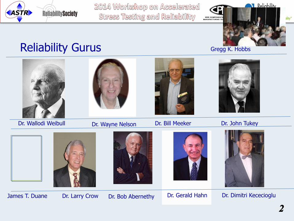
Reliability Gurus
Dr. John Tukey Dr. Wayne Nelson Dr. Bill Meeker
Dr. Gerald Hahn Dr. Bob Abernethy
Dr. Wallodi Weibull
Dr. Dimitri Kececioglu James T. Duane Dr. Larry Crow
Gregg K. Hobbs
Overview
1. Reliability Requirements and Decomposition
2. ALT Applications
3. Categories of ALT
4. ALT Models
5. Methodology (Weibull Analysis)
6. Test Strategies and Analysis
7. ALT and Reliability Growth
3
1. Reliability Requirement & Decomposition
4
• ALT is used in process of ensuring customer Reliability Requirements
• Good requirement writing practices need to apply to;
– Represent customer needs
– Avoid Scope Creep
– Robust across the product life (Cradle to Grave)
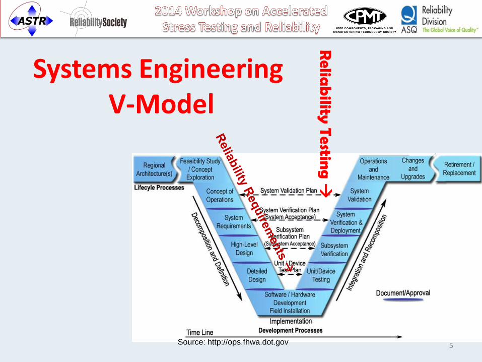
Systems Engineering V-Model
5 Source: http://ops.fhwa.dot.gov
Relia
bility Testin
g
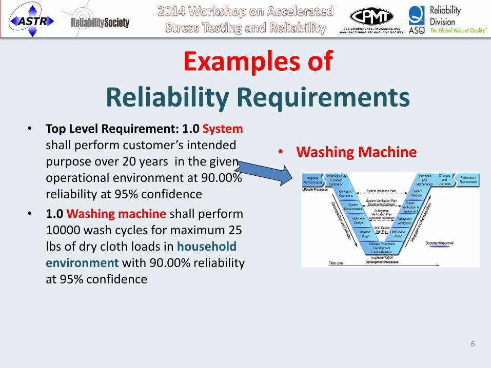
Examples of Reliability Requirements
• Top Level Requirement: 1.0 System shall perform customer’s intended purpose over 20 years in the given operational environment at 90.00% reliability at 95% confidence
• 1.0 Washing machine shall perform 10000 wash cycles for maximum 25 lbs of dry cloth loads in household environment with 90.00% reliability at 95% confidence
• Washing Machine
6
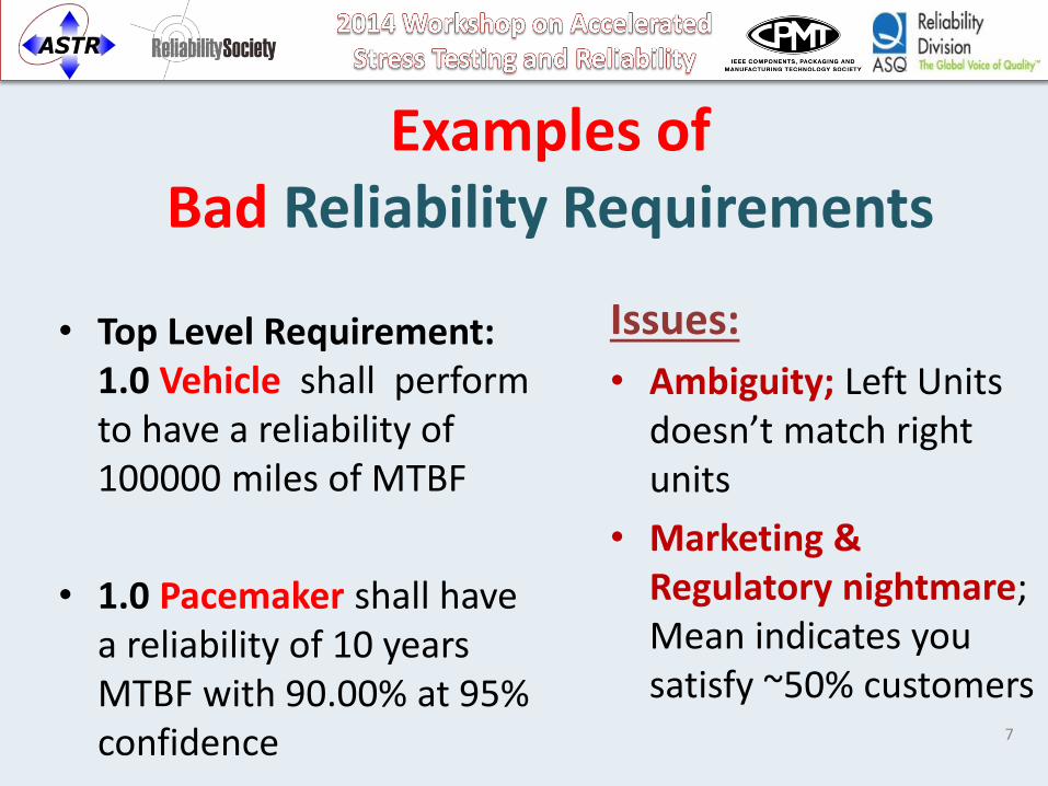
Examples of Bad Reliability Requirements
• Top Level Requirement: 1.0 Vehicle shall perform to have a reliability of 100000 miles of MTBF
• 1.0 Pacemaker shall have a reliability of 10 years MTBF with 90.00% at 95% confidence
7
Issues:
• Ambiguity; Left Units doesn’t match right units
• Marketing & Regulatory nightmare; Mean indicates you satisfy ~50% customers
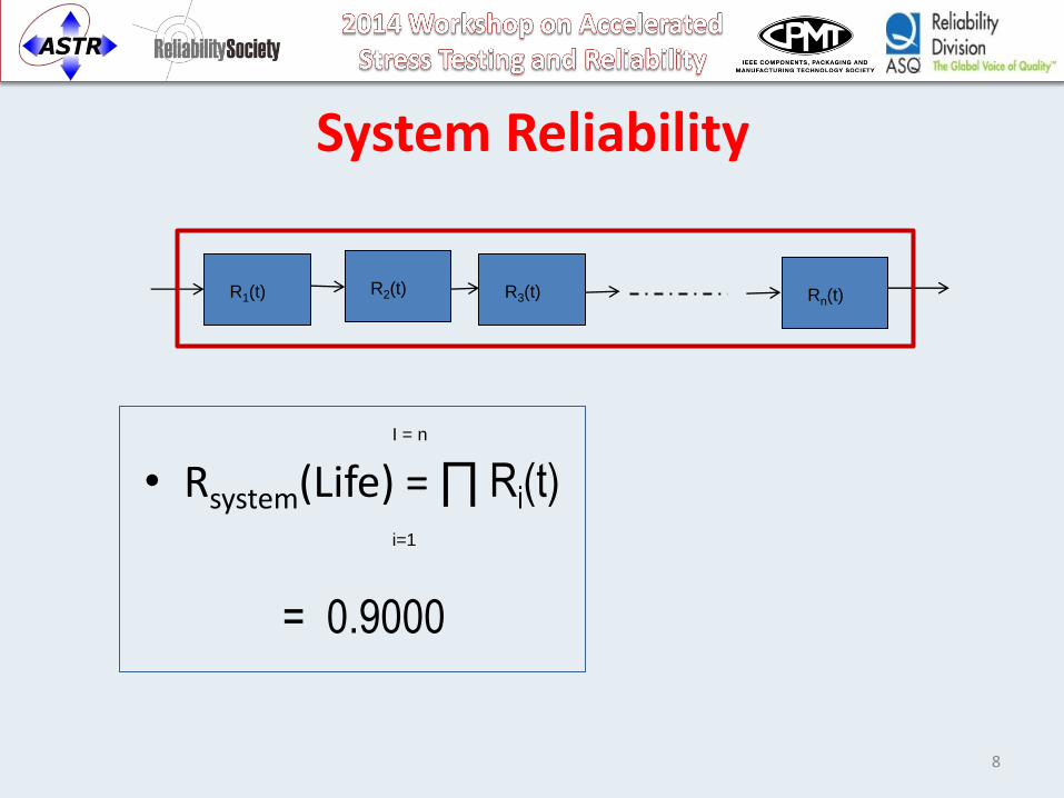
System Reliability
• Rsystem(Life) = ∏ Ri(t)
= 0.9000
8
R1(t)
R2(t)
R3(t)
Rn(t)
I = n
i=1
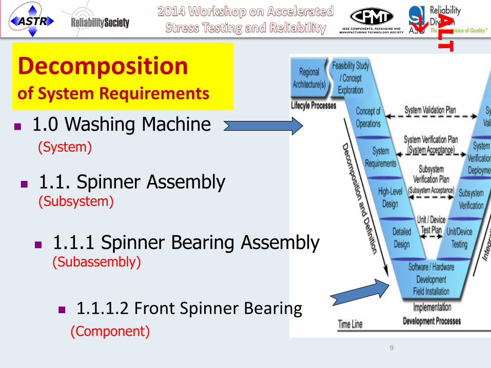
Decomposition of System Requirements
1.0 Washing Machine (System)
9
1.1. Spinner Assembly (Subsystem)
1.1.1 Spinner Bearing Assembly (Subassembly)
1.1.1.2 Front Spinner Bearing (Component)
ALT
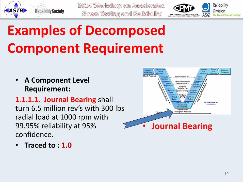
Examples of Decomposed Component Requirement
• A Component Level Requirement:
1.1.1.1. Journal Bearing shall turn 6.5 million rev’s with 300 lbs radial load at 1000 rpm with 99.95% reliability at 95% confidence.
• Traced to : 1.0
• Journal Bearing
10
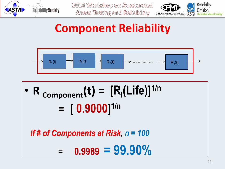
Component Reliability
• R Component(t) = [Ri(Life)]1/n
= [ 0.9000]1/n
If # of Components at Risk, n = 100
= 0.9989 = 99.90%
11
R1(t)
R2(t)
R3(t)
Rn(t)
2. ALT Applications
12
13
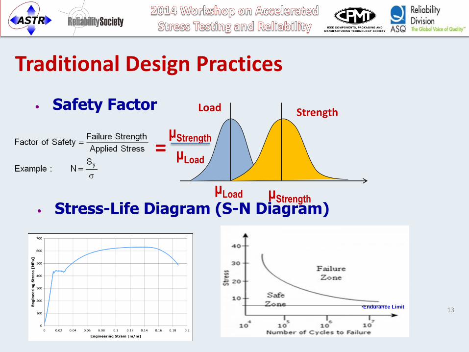
• Safety Factor
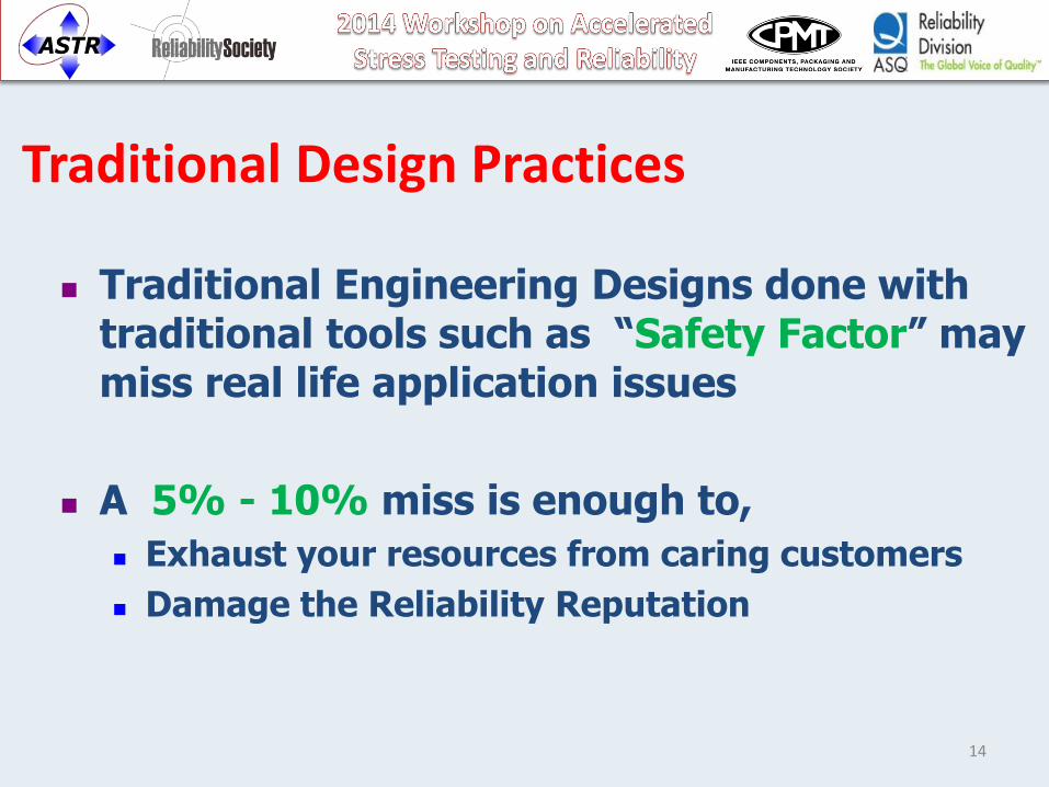
Traditional Design Practices
•Endurance Limit
• Stress-Life Diagram (S-N Diagram)
μLoad μStrength
Load Strength
μStrength
μLoad =
Traditional Design Practices
Traditional Engineering Designs done with traditional tools such as “Safety Factor” may miss real life application issues
A 5% - 10% miss is enough to,
Exhaust your resources from caring customers
Damage the Reliability Reputation
14

Factors Effecting Design Factor
Confidence
• How many will be produced?
• What manufacturing methods will be used?
• What are the consequences of failure? •Danger to people •Cost
• Size and weight important?
• What is the life of the component?
• Justify design expense?
• Temperature range.
• Exposure to electrical voltage or current.
• Susceptible to corrosion
• Is noise control important?
• Is vibration control important?
• Will the component be protected? •Guard •Housing
• Nature of the load considering all modes of operation:
• Startup, shutdown, normal operation, any foreseeable overloads
• Load characteristic • Static, repeated & reversed,
fluctuating, shock or impact
• Variations of loads over time.
• Magnitudes • Maximum, minimum, mean
Application
Environment Loads
• What kind of stress? • Direct tension or
compression • Direct shear • Bending • Torsional shear
• Application • Uniaxial • Biaxial • Triaxial
Types of Stresses
• Material properties
• Ultimate strength, yield strength, endurance strength,
• Ductility • Ductile: %E 5% • Brittle: %E < 5%
• Ductile materials are preferred for fatigue, shock or impact loads.
Material • Reliability of data for
• Loads • Material properties • Stress calculations
• How good is manufacturing quality control
• Will subsequent handling, use and environmental conditions affect the safety or life of the component?
15
16
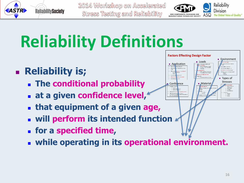
Reliability Definitions
Reliability is;
The conditional probability
at a given confidence level,
that equipment of a given age,
will perform its intended function
for a specified time,
while operating in its operational environment.
17
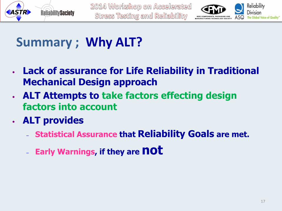
• Lack of assurance for Life Reliability in Traditional Mechanical Design approach
• ALT Attempts to take factors effecting design factors into account
• ALT provides
– Statistical Assurance that Reliability Goals are met.
– Early Warnings, if they are not
Summary ; Why ALT?
18
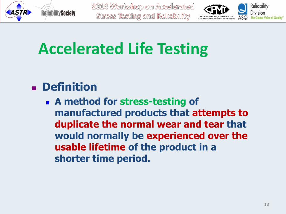
Accelerated Life Testing
Definition
A method for stress-testing of manufactured products that attempts to duplicate the normal wear and tear that would normally be experienced over the usable lifetime of the product in a shorter time period.
19
Accelerated Life Testing 1. Accelerate - cause (something) to happen sooner
– ac·cel·er·ate
– verb \-lə-ˌrāt\ : to move faster : to gain speed
– : to cause (something) to happen sooner or more quickly
2. Life - birth to death (Cradle to Grave!) – the period from birth to death – the period of duration, usefulness, or popularity of something <the
expected life of the batteries>
3. Testing – determine quality, or genuineness – noun – the means by which the presence, quality, or genuineness of
anything is determined; a means of trial. – the trial of the quality of something: to put to the test. – a particular process or method for trying or assessing.
20
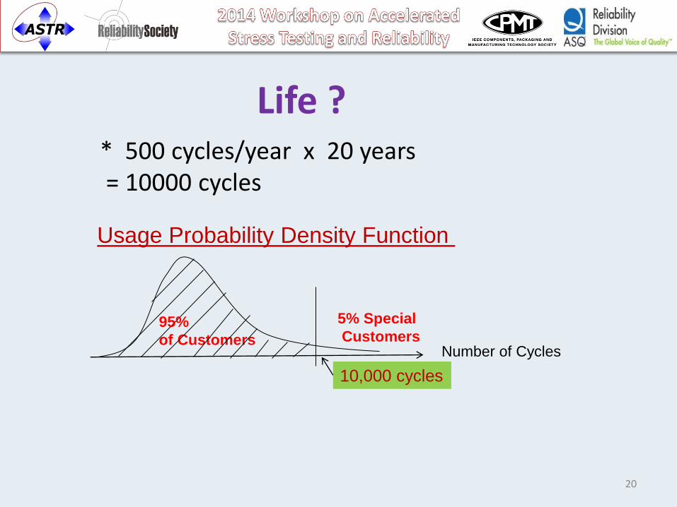
Life ? * 500 cycles/year x 20 years = 10000 cycles
95%
of Customers
10,000 cycles
Number of Cycles
Usage Probability Density Function
5% Special
Customers
21
Goals of ALT- Accelerated Life Testing
Most Important Goals of Up Front Product Life Testing (In-house or Beta Sites) & Data Analyses are
To gain information for Fundamental Improvements
Proactive Reliability Improvement before Product Release
22
HALT-Highly Accelerated Life Testing
A test in which stresses are applied to the product well beyond normal shipping, storage and in-use levels.
HALT is Scientific.
HALT has Statistical Differences with ALT
Advantages Quick Screening of Weak Products.
At Highly Stressed Levels, a few samples can be used. (Ex. Prototypes)
Compresses Design Time. Therefore, shortens the Design Iterations and Allow Mature Production.
23
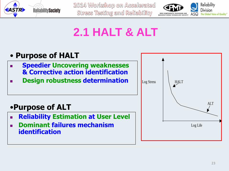
2.1 HALT & ALT
• Purpose of HALT
•Purpose of ALT
Speedier Uncovering weaknesses & Corrective action identification
Design robustness determination
Reliability Estimation at User Level
Dominant failures mechanism identification
Log Stress HALT
ALT
Log Life
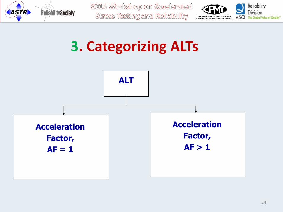
3. Categorizing ALTs
Acceleration
Factor,
AF = 1
ALT
Acceleration
Factor,
AF > 1
24
25
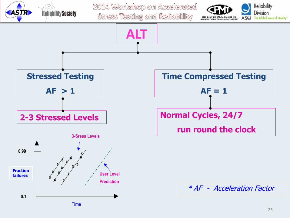
ALT
Stressed Testing
AF > 1
Time Compressed Testing
AF = 1
Normal Cycles, 24/7
run round the clock
2-3 Stressed Levels
* AF - Acceleration Factor
3-Sress Levels
0.99
User Level
Prediction
0.1
Time
Fraction failures
Acceleration Factor, AF = 1
User-Rate Acceleration
Many Products are not in Continuous Use.
So we Capitalize on them.
26
Acceleration Factor, AF = 1
User-Rate Acceleration
Advantages i) Results,
ii) Failure Modes,
iii) Sequence of Occurrences of Failure Modes are
Directly Correlated, therefore Analyses is easy
27
Acceleration Factor, AF = 1
User-Rate Acceleration
Disadvantages
Not applicable in every case.
Ex. Chemical Degradation
Corrosion in a Refrigerator-Door may not happen in a shorter time.
28
Acceleration Factor, AF > 1 - Case I
Exposing tests Units to more severe than normal Stresses. Ex.
Higher Temperature Higher Humidity Higher Vibration
To Accelerate Chemical/Physical Degradation
29
Acceleration Factor, AF > 1 - Case I
Accelerating Chemical/Physical Degradation Ex.
Weakening an Insulation of Motor Winding due to High Temperature and Moisture
Weakening the Lubricant in bearing with exposure to moisture and high Temperature
30
Acceleration Factor, AF > 1 - Case II
Product Stress Acceleration Load
Pressure
Ex of Results;
Wear, Fatigue Failures
31
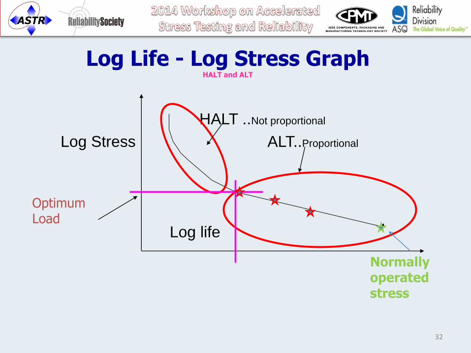
Log Life - Log Stress Graph
HALT and ALT
HALT ..Not proportional
Log Stress ALT..Proportional
Log life
Optimum Load
Normally operated stress
32
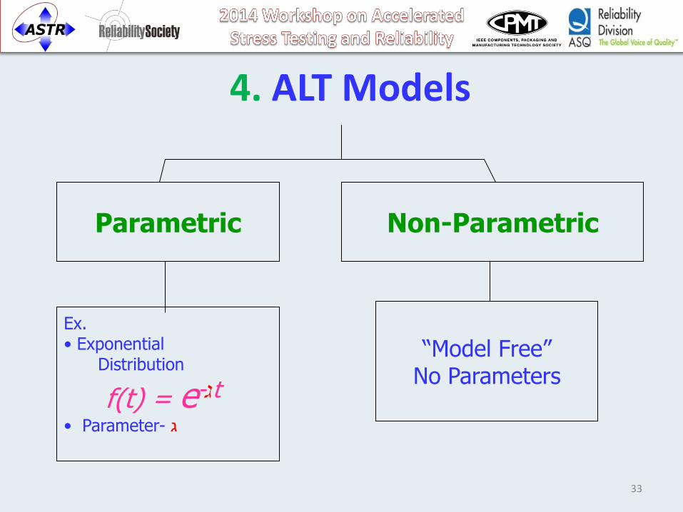
4. ALT Models
Parametric Non-Parametric
Ex. • Exponential Distribution
f(t) = e-גt
• Parameter- ג
“Model Free” No Parameters
33
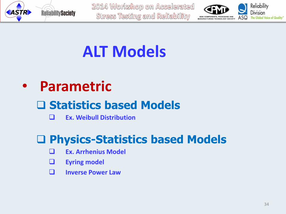
ALT Models
• Parametric Statistics based Models Ex. Weibull Distribution
Physics-Statistics based Models Ex. Arrhenius Model
Eyring model
Inverse Power Law
34
ALT Models
• Non-Parametric Statistics based Models
“Model Free” – Analyze as it is.
Ex. Proportional Hazard Rate
35
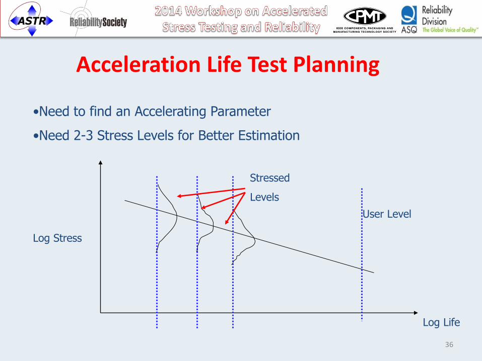
Acceleration Life Test Planning
Stressed
Levels
•Need to find an Accelerating Parameter
•Need 2-3 Stress Levels for Better Estimation
User Level
Log Life
Log Stress
36
37
5.
Methodology
Weibull Analysis
Reliability Plots
There are four important Reliability Plots.
If one of the four is known, rest can be found.
1. Probability Density Function - PDF, f(t)
2. Cum Distribution Function - CDF, F(t)
3. Reliability (Survival Function), R(t)
4. Bath-Tub Hazard Rate Function, h(t)
Next important plot is, 5) Cum Hazard function, H(t)
38
39
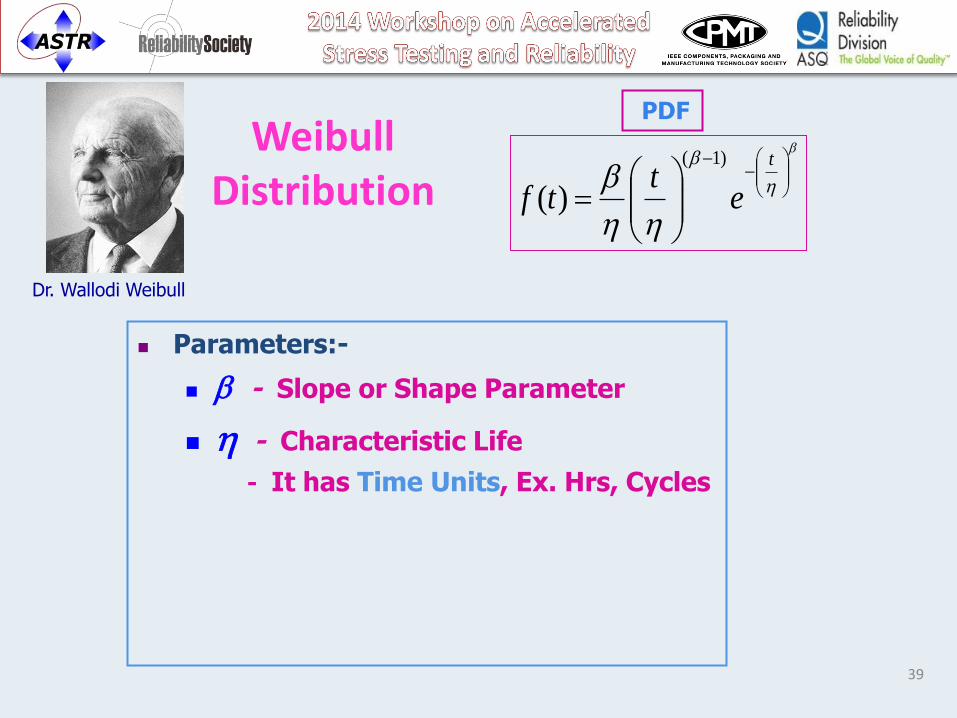
Weibull Distribution
Parameters:-
b - Slope or Shape Parameter
h - Characteristic Life
- It has Time Units, Ex. Hrs, Cycles
b
h
b
hh
b
t
et
tf
)1(
)(
Dr. Wallodi Weibull
40
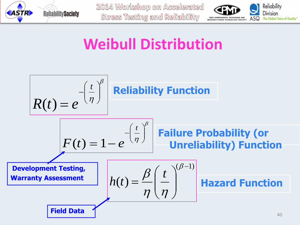
Weibull Distribution
Reliability Function b
h
t
etR )(b
h
t
etF 1)(
)1(
)(
b
hh
b tth
Failure Probability (or Unreliability) Function
Hazard Function
Development Testing,
Warranty Assessment
Field Data
41
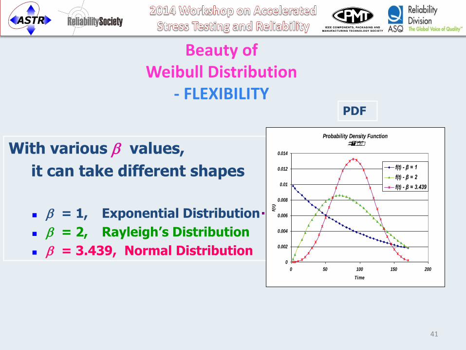
Beauty of Weibull Distribution
- FLEXIBILITY
With various b values,
it can take different shapes
b = 1, Exponential Distribution
b = 2, Rayleigh‟s Distribution
b = 3.439, Normal Distribution
Probability Density Function
h=100
0
0.002
0.004
0.006
0.008
0.01
0.012
0.014
0 50 100 150 200
Timef(
t)
f(t) - β = 1
f(t) - β = 2
f(t) - β = 3.439
42
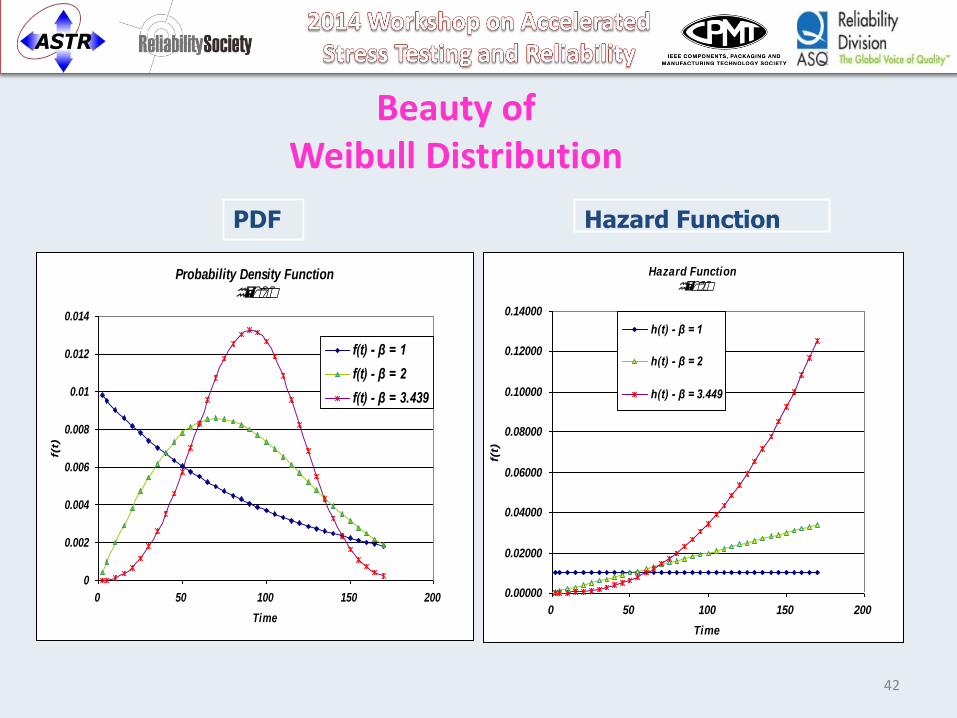
Beauty of Weibull Distribution
Probability Density Function
h=100
0
0.002
0.004
0.006
0.008
0.01
0.012
0.014
0 50 100 150 200
Time
f(t)
f(t) - β = 1
f(t) - β = 2
f(t) - β = 3.439
Hazard Function
h=100
0.00000
0.02000
0.04000
0.06000
0.08000
0.10000
0.12000
0.14000
0 50 100 150 200
Time
f(t)
h(t) - β = 1
h(t) - β = 2
h(t) - β = 3.449
Hazard Function PDF
43
6. Test Strategies and Analysis with
Weibull
44
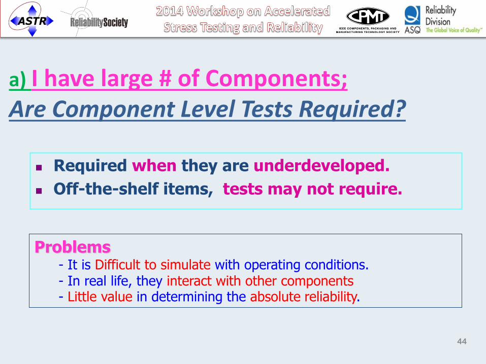
a) I have large # of Components; Are Component Level Tests Required?
Required when they are underdeveloped.
Off-the-shelf items, tests may not require.
Problems
- It is Difficult to simulate with operating conditions. - In real life, they interact with other components - Little value in determining the absolute reliability.
45
Solution: Test Subsystems ..!
Subsystem testing serves the purpose of
Subsystem Level Reliability Analysis
+ Component Level Reliability Analysis
Benefits. - Results are more relevant and accurate - Reduces the large # of component level testing.
46
Each failure mode has its own unique distributions.
If treated all as one, the result will be an unfit curve.
Right thing to do: „„Failure Mode-wise Reliability Analysis.‟‟
It is done by right censoring the data of other failure modes.
Benefits. - Focus on each failure mode, individually. - Find the impact on reliability growth, if fixed. - Justify resources allocation base on the impact.
b) Failure Mode-wise Reliability Analysis
47
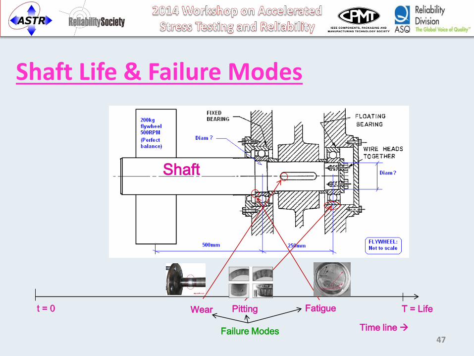
Shaft Life & Failure Modes
T = Life t = 0 Pitting Fatigue Wear
Shaft
Time line Failure Modes
48
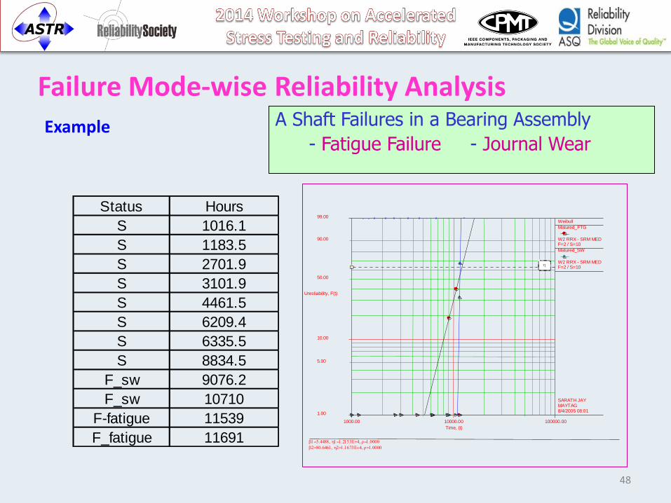
Failure Mode-wise Reliability Analysis Example
Status Hours
S 1016.1
S 1183.5
S 2701.9
S 3101.9
S 4461.5
S 6209.4
S 6335.5
S 8834.5
F_sw 9076.2
F_sw 10710
F-fatigue 11539
F_fatigue 11691
1000.00 100000.00 10000.00 1.00
5.00
10.00
50.00
90.00
99.00
h
Time, (t)
Unreliability, F(t)
8/4/2005 08:01 MAYTAG SARATH JAY
Weibull Matured_FTG W2 RRX - SRM MED F=2 / S=10
b h
Matured_SW W2 RRX - SRM MED F=2 / S=10
b h
A Shaft Failures in a Bearing Assembly
- Fatigue Failure - Journal Wear
49
c) Nearest Slope for the Improved “Zero Failure Design”
in Reliability Growth Monitoring
In PDP, when reliability improves, parts don‟t fail.
Improvements cause failures to delay.
The failure distribution‟s shape will remain unchanged.
Similar distributions carry same β - shape parameter.
Therefore, use the nearest slope for the β with zero failure
design.
50
1.00
5.00
10.00
50.00
90.00
99.90
1.00 10000.0010.00 100.00 1000.00Time Units
Unreliability,F(t)
2:53:01 PM10/1/2003MaytagSarath J
A
F=9 | S=0
b h
B
F=14 | S=0
b h
C
F=34 | S=2
b h
D
F=1 | S=14
b h
E
F=0 | S=14
b h
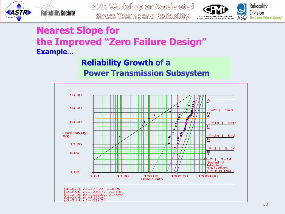
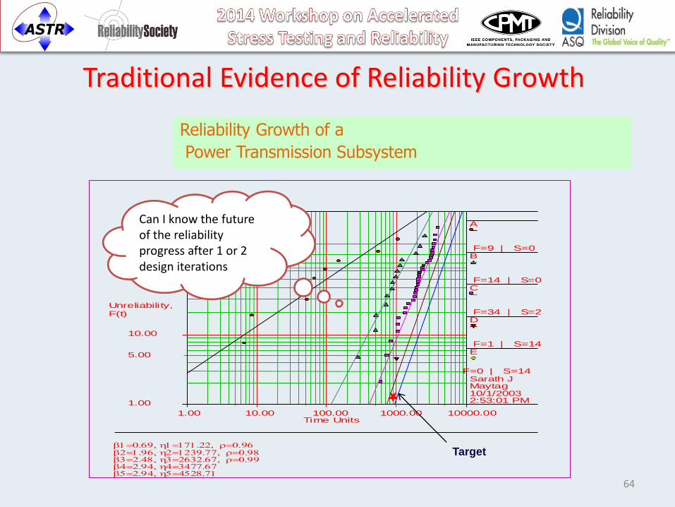
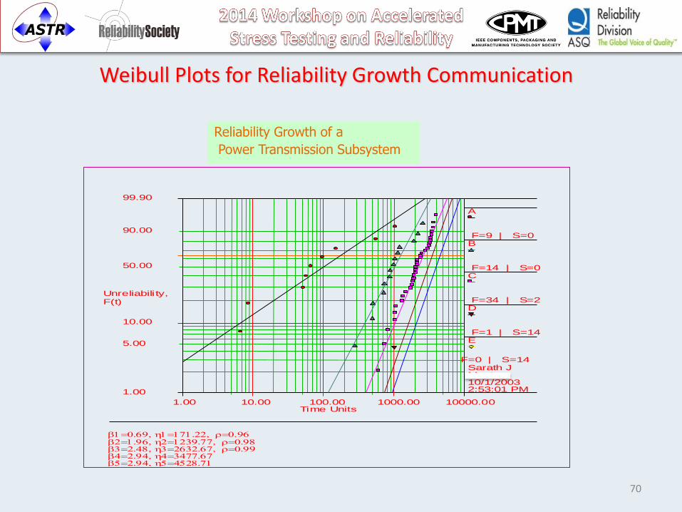
Reliability Growth of a
Power Transmission Subsystem
Nearest Slope for the Improved “Zero Failure Design” Example…
51
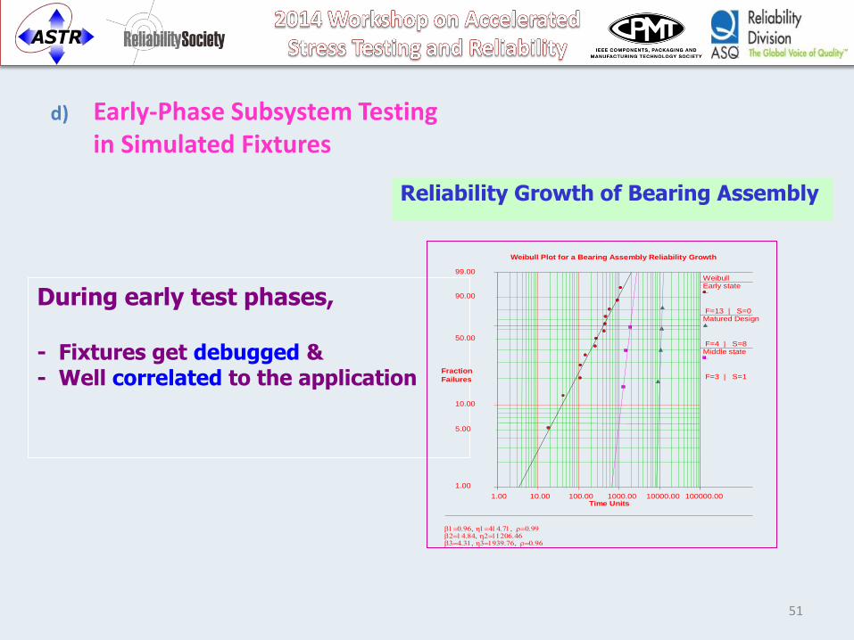
d) Early-Phase Subsystem Testing in Simulated Fixtures
During early test phases,
- Fixtures get debugged & - Well correlated to the application
Reliability Growth of Bearing Assembly
1.00
5.00
10.00
50.00
90.00
99.00
1.00 100000.0010.00 100.00 1000.00 10000.00
Weibull Plot for a Bearing Assembly Reliability Growth
Time Units
Fraction
Failures
WeibullEarly state
F=13 | S=0
b h
Matured Design
F=4 | S=8
b h
Middle state
F=3 | S=1
b h
52
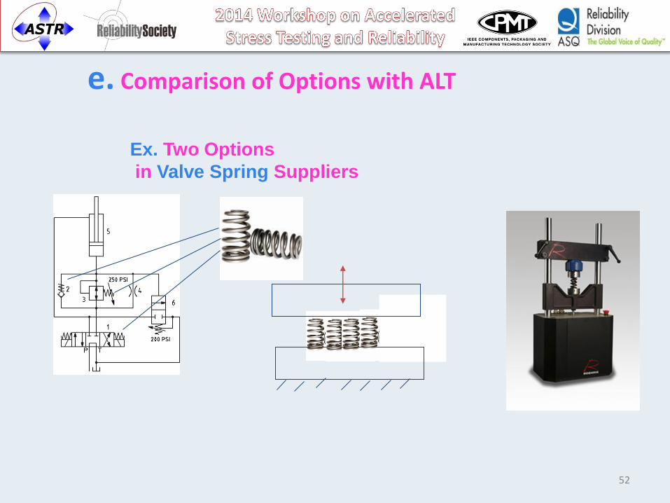
e. Comparison of Options with ALT
Ex. Two Options
in Valve Spring Suppliers
53
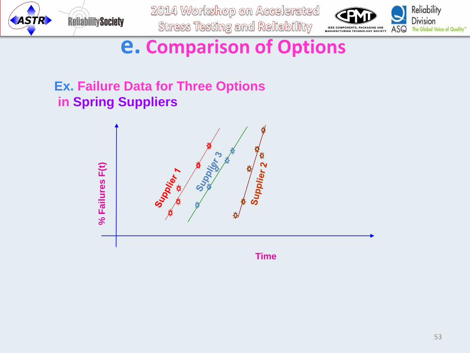
e. Comparison of Options
Ex. Failure Data for Three Options
in Spring Suppliers %
Fa
ilu
res
F(t
)
Time
54
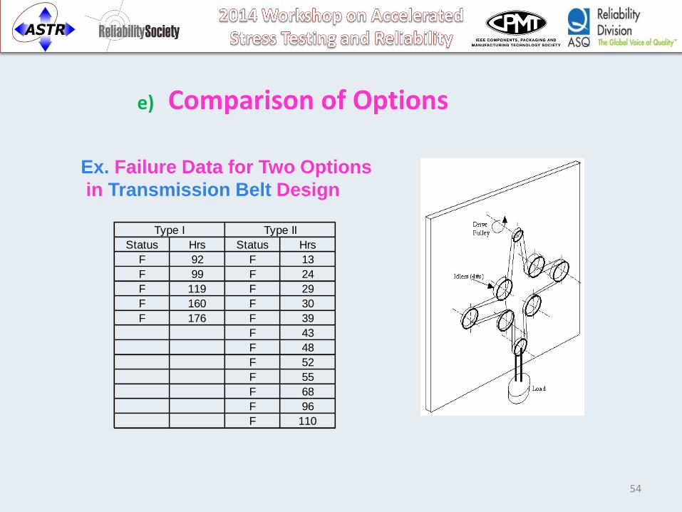
e) Comparison of Options
Status Hrs Status Hrs
F 92 F 13
F 99 F 24
F 119 F 29
F 160 F 30
F 176 F 39
F 43
F 48
F 52
F 55
F 68
F 96
F 110
Type I Type II
Ex. Failure Data for Two Options
in Transmission Belt Design
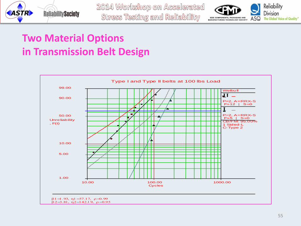
55
Two Material Options in Transmission Belt Design
1.00
5.00
10.00
50.00
90.00
99.00
10.00 1000.00100.00
Type I and Type II belts at 100 lbs Load
Cycles
Unreliability
, F(t)
Weibull
IIP=2, A=RRX-S F=12 | S=0
b h
IP=2, A=RRX-S F=5 | S=0
CB/FM: 95.00%
1 Sided-LC-Type 2
b h
56
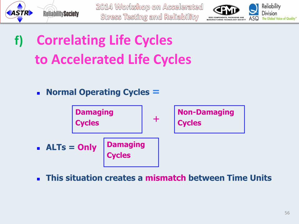
f) Correlating Life Cycles
to Accelerated Life Cycles
Normal Operating Cycles =
ALTs = Only
This situation creates a mismatch between Time Units
Damaging
Cycles
+
Non-Damaging
Cycles
Damaging
Cycles
57
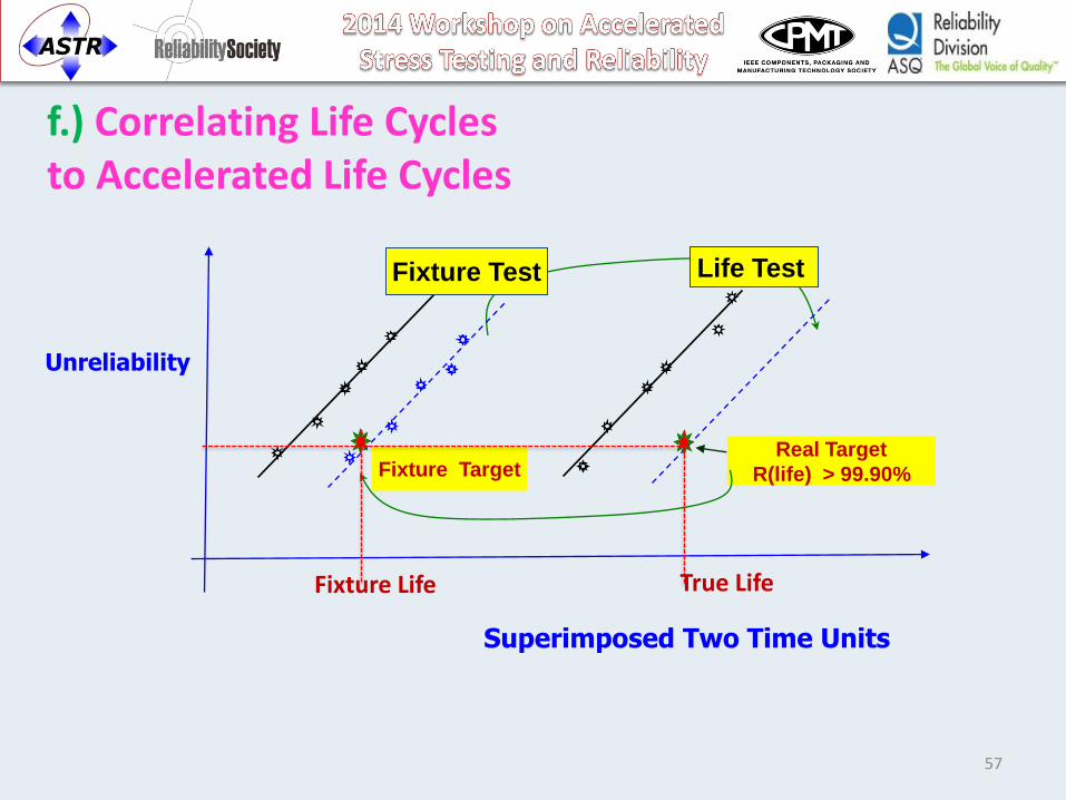
f.) Correlating Life Cycles to Accelerated Life Cycles
Superimposed Two Time Units
Fixture Test Life Test
Real Target
R(life) > 99.90% Fixture Target
Unreliability
True Life Fixture Life

58
Correlating Life Cycles to Accelerated Life Cycles
Example- A fatigue failure in a machine base
A late-life fatigue failure was discovered during time-compressed life testing.
A test fixture was made and reproduced the same failure in a very short time.
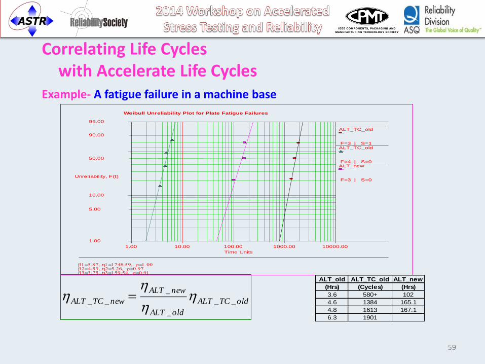
59
Correlating Life Cycles with Accelerate Life Cycles
Example- A fatigue failure in a machine base
1.00
5.00
10.00
50.00
90.00
99.00
1.00 10000.0010.00 100.00 1000.00
Weibull Unreliability Plot for Plate Fatigue Failures
Time Units
Unreliability, F(t)
ALT_TC_old
F=3 | S=1
b h
ALT_TC_old
F=4 | S=0
b h
ALT_new
F=3 | S=0
b h
ALT_old ALT_TC_old ALT_new
(Hrs) (Cycles) (Hrs)
3.6 580+ 102
4.6 1384 165.1
4.8 1613 167.1
6.3 1901
oldTCALT
oldALT
newALT
newTCALT __
_
_
__ hh
hh

7. ALT & Reliability Growth
60
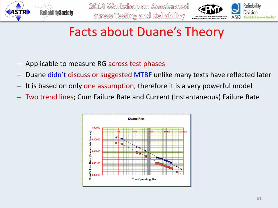
Facts about Duane’s Theory
– Applicable to measure RG across test phases
– Duane didn’t discuss or suggested MTBF unlike many texts have reflected later
– It is based on only one assumption, therefore it is a very powerful model
– Two trend lines; Cum Failure Rate and Current (Instantaneous) Failure Rate
61
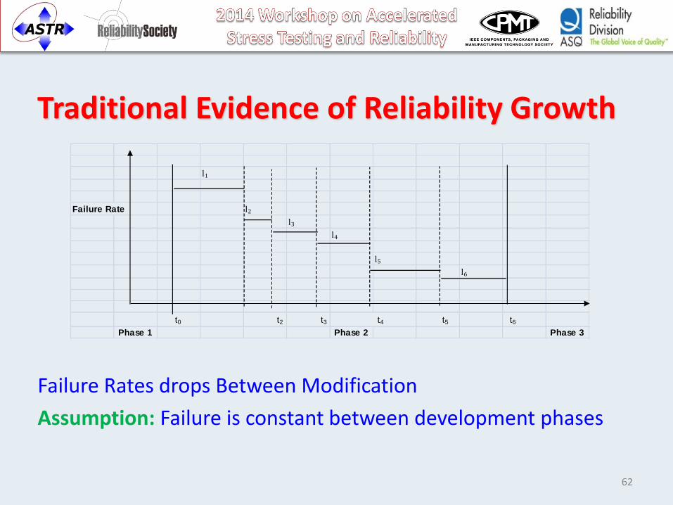
Traditional Evidence of Reliability Growth
Failure Rates drops Between Modification
Assumption: Failure is constant between development phases
l1
Failure Rate l2
l3
l4
l5
l6
t0 t1 t2 t3 t4 t5 t6
Phase 1 Phase 2 Phase 3
62
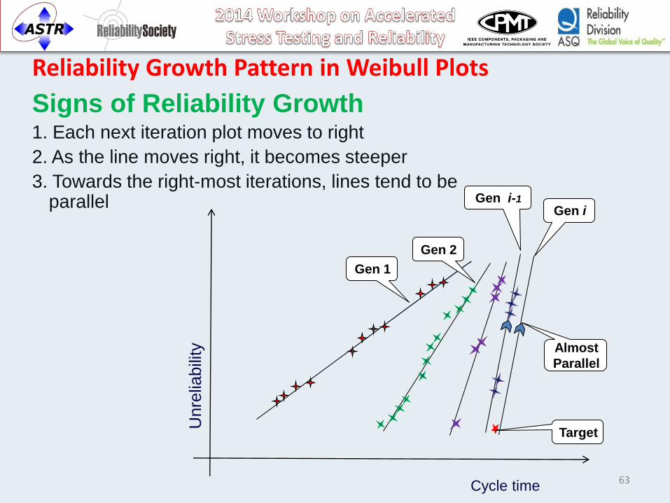
Reliability Growth Pattern in Weibull Plots
Unre
liabili
ty
Cycle time
Signs of Reliability Growth 1. Each next iteration plot moves to right
2. As the line moves right, it becomes steeper
3. Towards the right-most iterations, lines tend to be parallel
Gen 1
Gen 2
Gen i-1
Gen i
Almost
Parallel
Target
63
1.00
5.00
10.00
50.00
90.00
99.90
1.00 10000.0010.00 100.00 1000.00Time Units
Unreliability,F(t)
2:53:01 PM10/1/2003MaytagSarath J
A
F=9 | S=0
b h
B
F=14 | S=0
b h
C
F=34 | S=2
b h
D
F=1 | S=14
b h
E
F=0 | S=14
b h
Reliability Growth of a
Power Transmission Subsystem
Traditional Evidence of Reliability Growth
Can I know the future of the reliability progress after 1 or 2 design iterations
Target
64

Duane provided the Predictions from early learning
Base Assumption:
• Repeatable trends occur during development cycles.
I. These trends provide the basis for a learning curve
II. Extremely useful in; a) Monitoring the progress of reliability improvement
b) Predicting the duration and end result of such program
65
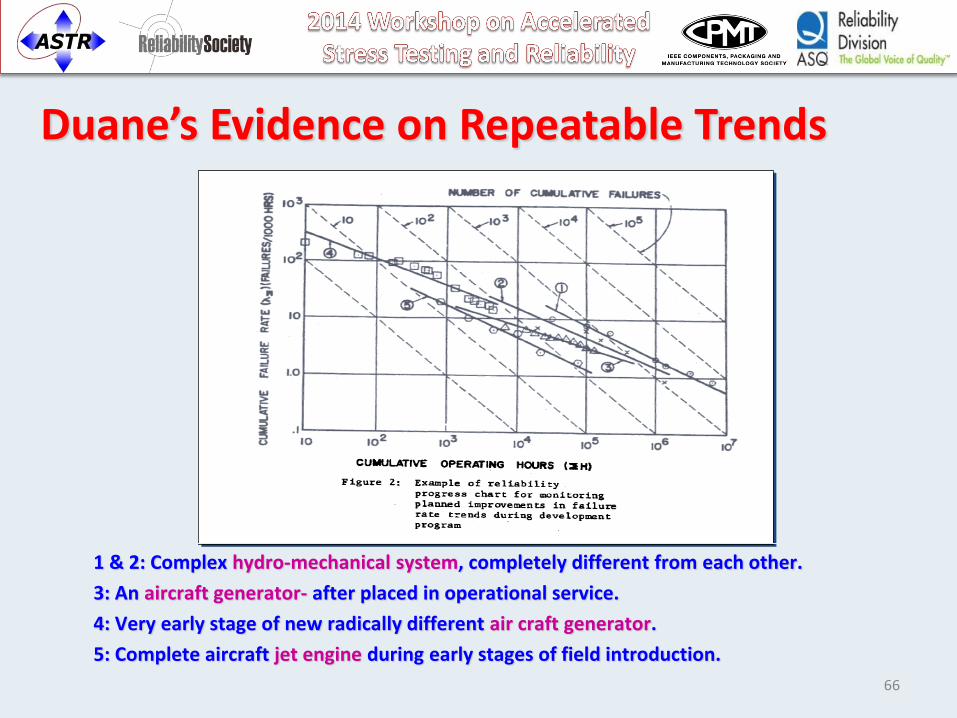
Duane’s Evidence on Repeatable Trends
1 & 2: Complex hydro-mechanical system, completely different from each other.
3: An aircraft generator- after placed in operational service.
4: Very early stage of new radically different air craft generator.
5: Complete aircraft jet engine during early stages of field introduction.
66
67
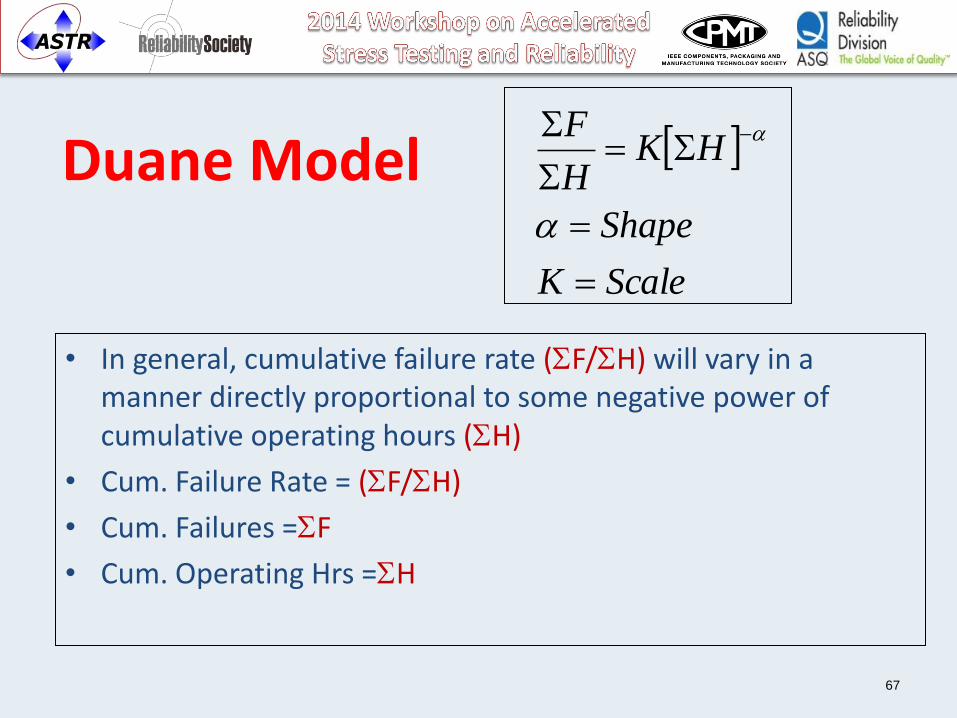
Duane Model
• In general, cumulative failure rate (SF/SH) will vary in a manner directly proportional to some negative power of cumulative operating hours (SH)
• Cum. Failure Rate = (SF/SH)
• Cum. Failures =SF
• Cum. Operating Hrs =SH
ScaleK
Shape
HKH
F
SS
S
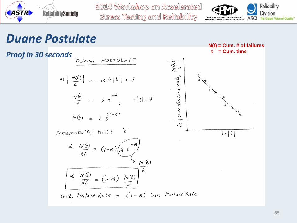
Duane Postulate Proof in 30 seconds
N(t) = Cum. # of failures
t = Cum. time
68
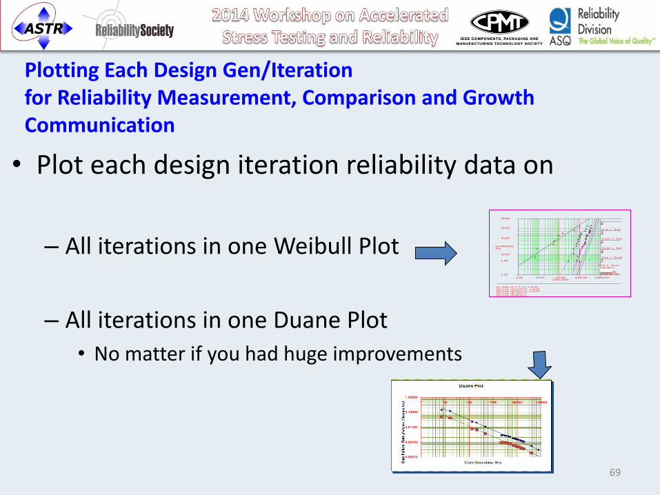
Plotting Each Design Gen/Iteration for Reliability Measurement, Comparison and Growth Communication
• Plot each design iteration reliability data on
– All iterations in one Weibull Plot
– All iterations in one Duane Plot
• No matter if you had huge improvements
1.00
5.00
10.00
50.00
90.00
99.90
1.00 10000.0010.00 100.00 1000.00Time Units
Unreliability,F(t)
2:53:01 PM10/1/2003MaytagSarath J
A
F=9 | S=0
b h
B
F=14 | S=0
b h
C
F=34 | S=2
b h
D
F=1 | S=14
b h
E
F=0 | S=14
b h
69
1.00
5.00
10.00
50.00
90.00
99.90
1.00 10000.0010.00 100.00 1000.00Time Units
Unreliability,F(t)
2:53:01 PM10/1/2003MaytagSarath J
A
F=9 | S=0
b h
B
F=14 | S=0
b h
C
F=34 | S=2
b h
D
F=1 | S=14
b h
E
F=0 | S=14
b h
Reliability Growth of a
Power Transmission Subsystem
Weibull Plots for Reliability Growth Communication
70

Duane Model Example for the Transmission
using individual data across Development Program
Y = -0.5947X - 0.6933 R2 = 0.9946
Overall slope
gives the vigor of
the program
Target
71
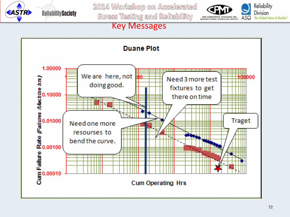
72
Key Messages
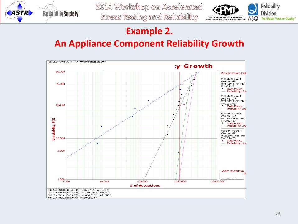
Example 2. An Appliance Component Reliability Growth
ReliaSoft Weibull++ 7 - www.ReliaSoft.com
Lid Lock Reliability Growth
Folio1\Phase 4: b h
Folio1\Phase 3: b h
Folio1\Phase 2: b h
Folio1\Phase 1: b h
# of Actuations
Unr
elia
bilit
y, F
(t)
1.000 10000.00010.000 100.000 1000.0001.000
5.000
10.000
50.000
90.000
99.000Probability-Weibull
Folio1\Phase 1Weibull-2PRRX SRM MED FMF=6/S=3
Data PointsProbability Line
Folio1\Phase 2Weibull-2PRRX SRM MED FMF=13/S=1
Data PointsProbability Line
Folio1\Phase 3Weibull-2PRRX SRM MED FMF=2/S=13
Data PointsProbability Line
Folio1\Phase 4Weibull-1PMLE SRM MED FMF=1/S=33
Data PointsProbability Line
Sarath jayatillekaBeckman Coulter Inc11/05/20103:59:07 PM
73
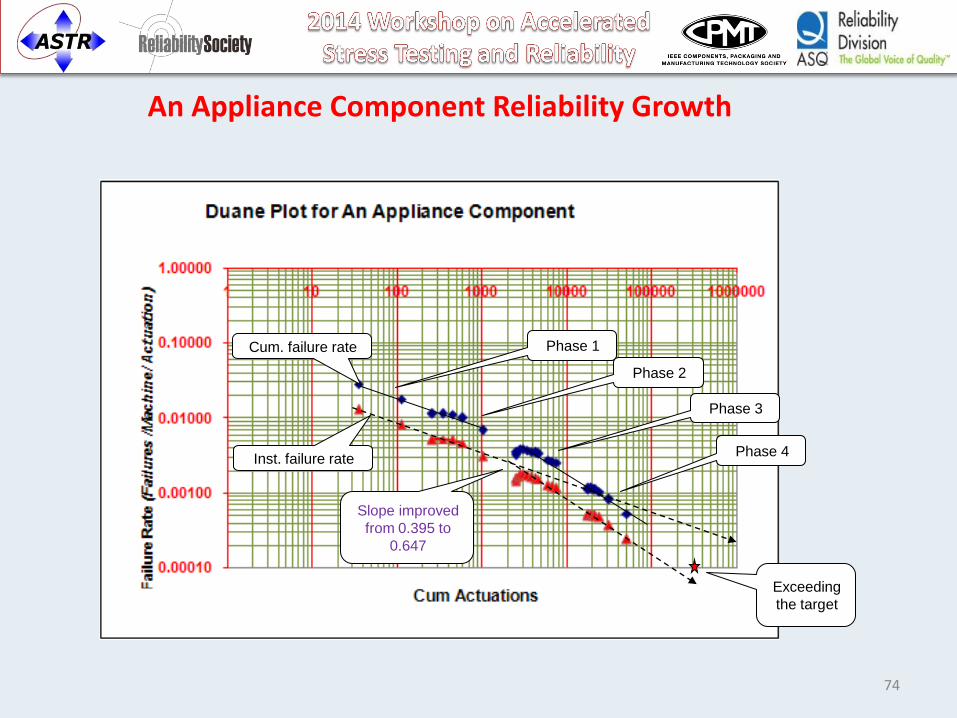
An Appliance Component Reliability Growth
Phase 1
Phase 3
Phase 4
Exceeding
the target
Phase 2
Slope improved
from 0.395 to
0.647
Cum. failure rate
Inst. failure rate
74
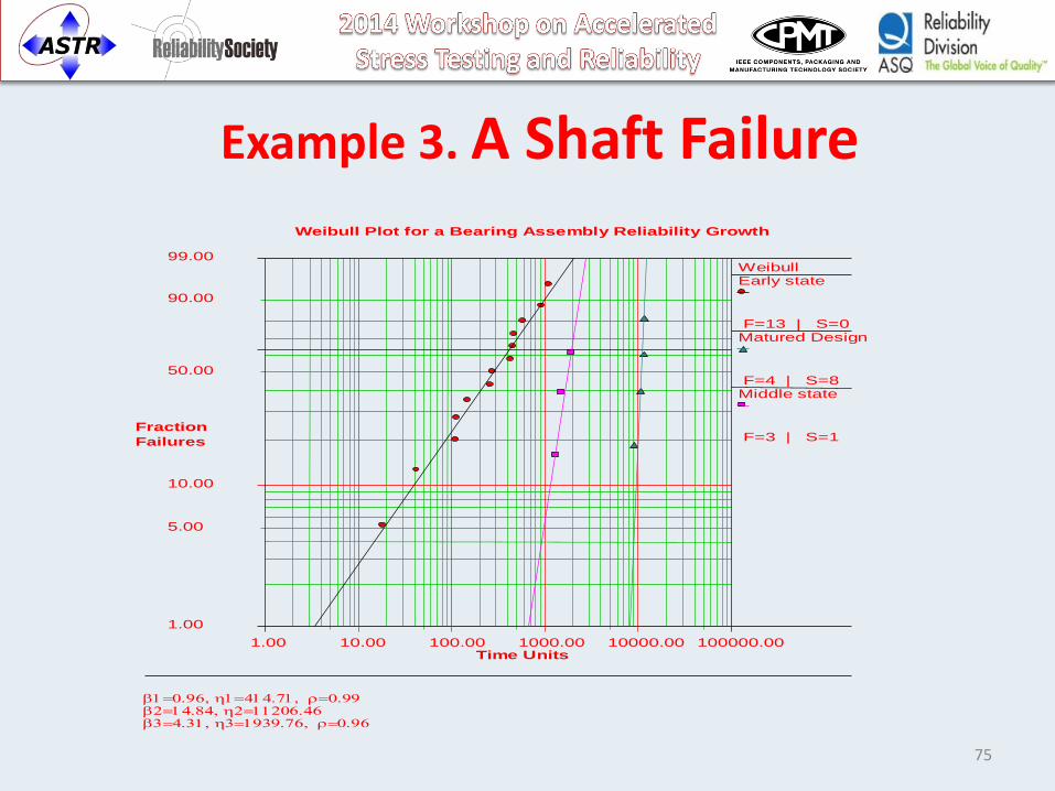
Example 3. A Shaft Failure
1.00
5.00
10.00
50.00
90.00
99.00
1.00 100000.0010.00 100.00 1000.00 10000.00
Weibull Plot for a Bearing Assembly Reliability Growth
Time Units
Fraction
Failures
WeibullEarly state
F=13 | S=0
b h
Matured Design
F=4 | S=8
b h
Middle state
F=3 | S=1
b h
75
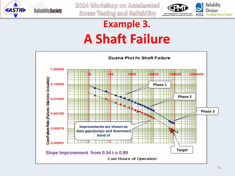
Example 3.
A Shaft Failure
Phase 1
Phase 2
Phase 3
Improvements are shown as
data gaps/jumps and downward
bend of
Target Slope Improvement from 0.54 t o 0.89
76

77
Thank You
Recommended