Accounting-Based Valuation Slides
James P. Sinclair
University of Connecticut
Spring 2015

Discussion
On July 31, 2009, Huron Consulting (Ticker: HURN) announced its intention to
restate their financial statements for fiscal years 2006, 2007, 2008, and Q1 2009. The
restatement pertained to non-cash acquisition-related charges (ironically, Huron is a
financial consulting firm offering advisory services in many areas, including
acquisitions). Upon hearing news of a pending restatement, trading volume in HURN
spiked and price plummeted, dropping nearly 70% in one day.
1. What factors may have prevented Huron’s auditors from detecting the
misstatement earlier?
2. What incentives did Huron’s managers have to misreport their financials? Be
specific.
3. Review Huron’s 2009 unadjusted 10-K. In retrospect, can you identify any
clues/red flags that a sophisticated user of financial statements may have been
able to identify prior to the restatement announcement?

Discussion
Valuation models, estimates, forecasts, and inputs vary widely across users. For example, two
distinct sources recently published their results attempting to value collegiate football
programs. Forbes valued the University of Texas Longhorns’ football team at $131 million.
Ryan Brewer, an Indiana University assistant professor of finance, valued the same team at
$972 million.
1. As best as you can, research the valuation methodologies used by each source. In your opinion, which
source (Forbes or Brewer) published the more accurate valuation? Are both sources way off the mark?
Are both sources close to the team’s intrinsic value? Defend your response.
2. What incentives to publish ‘accurate’ figures are present for each source? Can you identify any
potential biases that may influence either source to distort their findings?
3. Develop you own model for valuing collegiate football programs. What inputs would go into your
model? From where would you collect your data? In an ideal setting, what (perhaps currently
unavailable) data would be useful to you in deriving a value for this asset?

Discussion
Consider the following three events:
• On December 15, 2005, an ice storm caused power outages to 683,000 electrical customers in North
Carolina and South Carolina. Power was not fully restored until six days later. Fifty-seven (57) firms
were headquartered in the blackout area.
• On September 19, 2008, the SEC took ‘emergency action’ and temporarily banned investors from
short-selling over 750 financial companies. This ban effectively limited the ability of pessimistic
investors to borrow shares with the intention of selling them, then buy them back at some point in the
future (i.e., betting on the stock’s price to decline). This ban was lifted 19 days later, on October 8,
2008.
• On April 23, 2013, at 1:07pm, hackers hijacked the Associated Press Twitter account and posted the
following message: “Breaking: Two Explosions in the White House and Barack Obama is injured”. At
the time, the AP Twitter account had nearly two million followers. By 1:10pm (just three minutes
later), the hoax had been revealed as fraudulent.
1. What effect do you think each event had on stock prices? Why?
2. What effect do you think each event had on intrinsic values (for the affected firms)? Why?
3. Social media has become a powerful tool in making investment decisions; yet, recent attacks have called into
question its reliability. How can sophisticated investors (or managers) effectively employ social media in making
investment decisions without falling victim to misinformation or vicious hoaxes?
Framework for Financial Statement Analysis
The primary reason for performing financial statement
analysis is to facilitate an economic decision
Framework
1. Establish objectives
2. Collect data
3. Process data
4. Conduct analyses
5. Develop recommendations and communicate results
6. Review

Who uses Financial Statements?
• Investors
• Managers
• Customers
• Suppliers
• Creditors
• Government regulators
• Employee unions
• Public interest groups
Sources of Information
Firm
Annual report (including MD&A, Auditor’s report, financial statements, and notes)
Other SEC filings (e.g., 10-q, 8-k, 4)
Voluntary disclosures (e.g., management forecasts)
Investor Relations site
Price / Volume charts
Social media???
External
Ownership reports (e.g., 13f, NQ)
Analyst reports / recommendations
Business periodicals (i.e., newspapers, newsletters, magazines)
Investment advisory services (i.e., S&P, Moody’s)
Industry
Industry reports
Macro economy
Risk-free rate, treasury rates
Unemployment
GDP
Corporate Financial Reporting
• What are the most important measures reported to outsiders?
• What are the most important earnings benchmarks?
• Why meet earnings benchmarks?
• What happens if earnings benchmarks are missed?
• What actions may be taken near the end of the quarter to boost earnings?
• Are smooth earnings important? Why?
• Why disclose voluntary information?
• Why avoid disclosing voluntary information?
See Graham, J.R., Harvey, C.R., Rajgopal, S., 2005. The economic implications of corporate financial
reporting. Journal of Accounting and Economics 40, 3-73 for a nice discussion of these topics.

Accounting Today – Top 100 Firms
2011 2014

What do Valuation Professionals Evaluate?
• Asset retirement obligations
• Brand equity
• Business enterprises
• Copyrights
• Customer relationships
• Employment agreements
• Financial instruments
• Goodwill
• Intellectual property
• Patents
• Pensions
• Real Estate
• Securities
• Stock-based compensation
• Trademarks
• and more…
Transactions, tax reporting, financial reporting, litigation, etc.
What do Valuation Professionals Need to Know?
• Accounting
• Best practices in valuation
• Capital structure
• Corporate governance
• Economics
• Financial Statement Analysis
• Growth analysis
• Industry information
• Legal environment
• Management strategy
• Regulatory standards
• Statistics
• Taxes (federal, state, local)
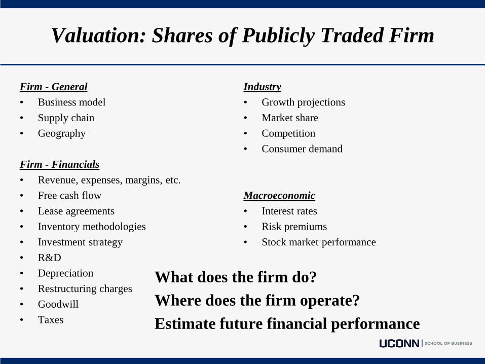
Valuation: Shares of Publicly Traded Firm
Firm - General
• Business model
• Supply chain
• Geography
Firm - Financials
• Revenue, expenses, margins, etc.
• Free cash flow
• Lease agreements
• Inventory methodologies
• Investment strategy
• R&D
• Depreciation
• Restructuring charges
• Goodwill
• Taxes
Industry
• Growth projections
• Market share
• Competition
• Consumer demand
Macroeconomic
• Interest rates
• Risk premiums
• Stock market performance
What does the firm do?
Where does the firm operate?
Estimate future financial performance

Simple Example
Firm A Firm B
$40 Stock Price $40
$10 Reported EPS $10
4x PE ratio 4x
Two nearly identical firms:
Consider the following scenarios:
1) Inventory valuation: Firm A uses FIFO; Firm B uses LIFO – costs are rising
2) Lease accounting: Firm B always includes bargain purchase option on leased
property; Firm A does not (assume no other capital lease conditions are met and
lease expense < depreciation)
3) Restructuring charges: Firm B took a one-time charge
4) Analyst estimates: EPS forecast for Firm A = $10.00; Firm B = $11.00
5) CEO characteristics: CEO for Firm A is in her last year and bonus is contingent on
meeting or beating analyst forecasts; CEO for Firm B is in early stages of career and
bonus is contingent on future growth
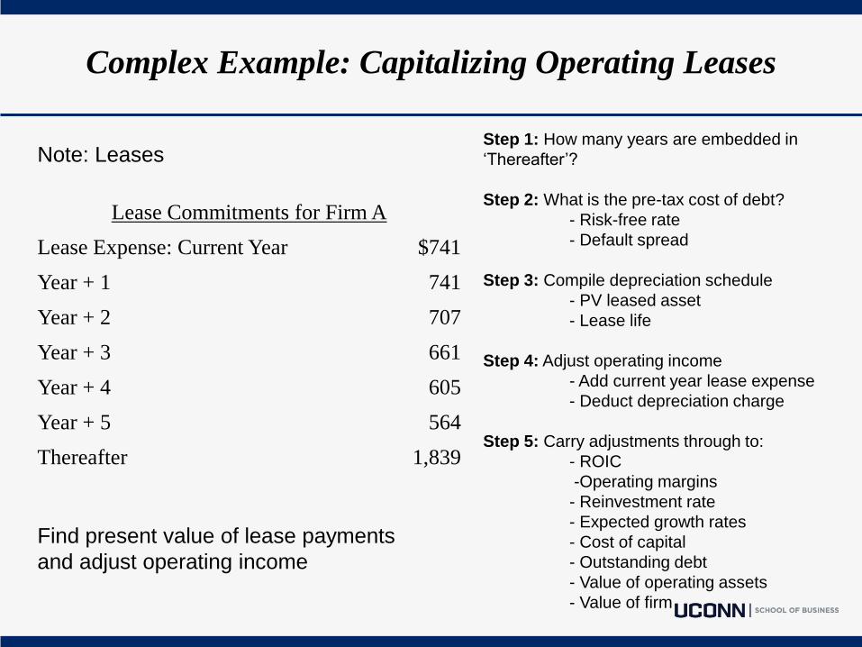
Complex Example: Capitalizing Operating Leases
Lease Commitments for Firm A
Lease Expense: Current Year $741
Year + 1 741
Year + 2 707
Year + 3 661
Year + 4 605
Year + 5 564
Thereafter 1,839
Note: Leases
Find present value of lease payments
and adjust operating income
Step 1: How many years are embedded in
‘Thereafter’?
Step 2: What is the pre-tax cost of debt?
- Risk-free rate
- Default spread
Step 3: Compile depreciation schedule
- PV leased asset
- Lease life
Step 4: Adjust operating income
- Add current year lease expense
- Deduct depreciation charge
Step 5: Carry adjustments through to:
- ROIC
-Operating margins
- Reinvestment rate
- Expected growth rates
- Cost of capital
- Outstanding debt
- Value of operating assets
- Value of firm

Market Efficiency
Why value a firm that already has a stock price?
Are markets efficient?
What factors must exist to consider a market to be ‘efficient’?

The Efficient Market Hypothesis (EMH)
In an efficient market, prices reflect all available information
Notice that the level / degree/ form of efficiency in a market depends upon two dimensions:
• The type of information incorporated into price
(what information is “available”)
• The speed with which new information is incorporated into price
(how fast information is “reflected”)

Why are we Interested in Market Efficiency?
• If market prices reflect only information of a particular type at a given date, then one can profit
by trading based on information relevant for pricing but not yet reflected in prices
• To assess the level of market efficiency we need to know the security’s value; which requires
knowing how assets are priced
• Joint-Test Problem in Empirical Tests of the EMH:
Market Efficiency per se is not testable because the question whether price reflects a given
piece of information always depends on the asset pricing model being used. It is always a
joint test of market efficiency and the pricing model.
• Despite the joint-test problem, tests of market efficiency (i.e., scientific search for inefficiencies)
improves our understanding of the behavior of returns across time and securities. It helps to
improve existing asset pricing models and the view and practices of financial market
professionals

Categories of Market Efficiency
Weak-Form Efficiency
• Price reflects all information contained in market trading data (past prices, volume, dividends,
interest rates, etc.).
Implication: Investors cannot use past prices to identify mispriced securities.
Note: Technical analysis refers to the practice of using past patterns in stock prices (and trades)
to identify future patterns in prices. This strategy is not profitable in a market which is at least
weak-form efficient.
Semi-Strong-Form Efficiency
• Price reflects all publicly available information.
Implication: Investors cannot use publicly available information to identify mispriced securities.
Note: Fundamental analysis refers to the practice of using financial statements, announcements,
and other publicly available information about firms to pick stocks. This strategy is not
profitable in a market which is at least semi-strong form efficient. If a market is semi-strong
form efficient, then it is also weak-form efficient since past prices and other past trading data are
publicly available
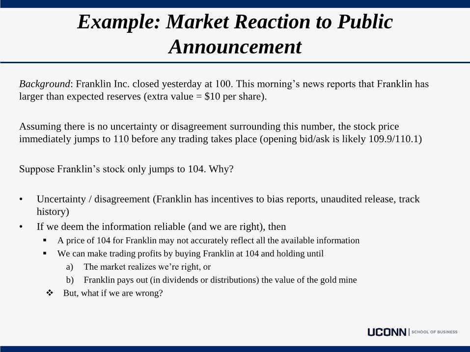
Example: Market Reaction to Public
Announcement
Background: Franklin Inc. closed yesterday at 100. This morning’s news reports that Franklin has
larger than expected reserves (extra value = $10 per share).
Assuming there is no uncertainty or disagreement surrounding this number, the stock price
immediately jumps to 110 before any trading takes place (opening bid/ask is likely 109.9/110.1)
Suppose Franklin’s stock only jumps to 104. Why?
• Uncertainty / disagreement (Franklin has incentives to bias reports, unaudited release, track
history)
• If we deem the information reliable (and we are right), then
A price of 104 for Franklin may not accurately reflect all the available information
We can make trading profits by buying Franklin at 104 and holding until
a) The market realizes we’re right, or
b) Franklin pays out (in dividends or distributions) the value of the gold mine
But, what if we are wrong?
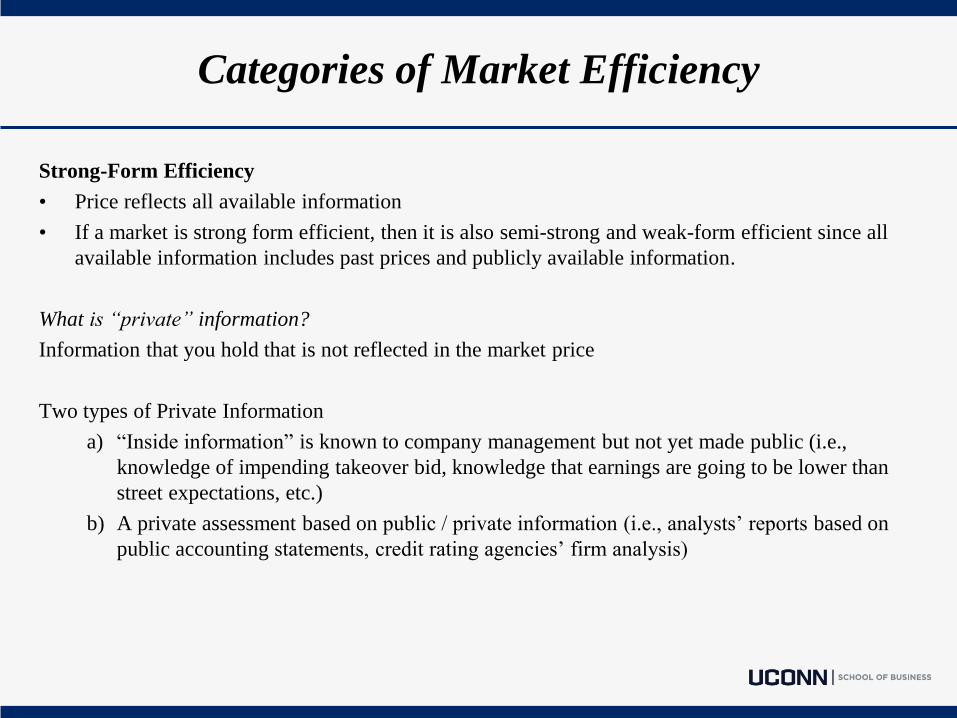
Categories of Market Efficiency
Strong-Form Efficiency
• Price reflects all available information
• If a market is strong form efficient, then it is also semi-strong and weak-form efficient since all
available information includes past prices and publicly available information.
What is “private” information?
Information that you hold that is not reflected in the market price
Two types of Private Information
a) “Inside information” is known to company management but not yet made public (i.e.,
knowledge of impending takeover bid, knowledge that earnings are going to be lower than
street expectations, etc.)
b) A private assessment based on public / private information (i.e., analysts’ reports based on
public accounting statements, credit rating agencies’ firm analysis)

Example
Private information can be impounded into the security price via reported trades
Background: Franklin Inc. closed yesterday at 100. Today’s opening bid/ask is 99.9/100.1. We
overhear two professors talking on the train: “Franklin has larger than expected reserves (extra value
= $10 per share).”
So, we begin to buy at the ask (100.1). Quotes are revised to 100 (bid)/100.2 (ask).
We buy more at 100.2. Quotes are again revised, and so on…
If we have the resources, we’ll stop buying only when the price reaches 110.
When price equals 110, the private information is fully reflected
Note that the market reaction is not driven directly by the private information, but instead by
trading activity.
Traders profit at the expense of other market participants.
Insider Trading
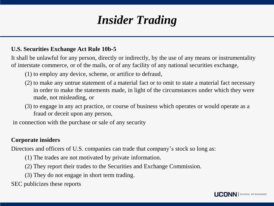
U.S. Securities Exchange Act Rule 10b-5
It shall be unlawful for any person, directly or indirectly, by the use of any means or instrumentality
of interstate commerce, or of the mails, or of any facility of any national securities exchange,
(1) to employ any device, scheme, or artifice to defraud,
(2) to make any untrue statement of a material fact or to omit to state a material fact necessary
in order to make the statements made, in light of the circumstances under which they were
made, not misleading, or
(3) to engage in any act practice, or course of business which operates or would operate as a
fraud or deceit upon any person,
in connection with the purchase or sale of any security
Corporate insiders
Directors and officers of U.S. companies can trade that company’s stock so long as:
(1) The trades are not motivated by private information.
(2) They report their trades to the Securities and Exchange Commission.
(3) They do not engage in short term trading.
SEC publicizes these reports

Five Steps to Discounted Cash Flow Valuation
Before you start, choose asset to value. Recognize and identify as many preconceived biases and
assumptions that may influence your valuation.
1. Estimate the discount rate(s) to use in the valuation
a. Cost of equity or cost of capital
b. Discount rates can vary over time
2. Estimate current earnings and cash flows
3. Estimate future earnings and cash flows
4. Estimate when the firm will reach stable growth; and what will the firm’s risk and cash flows
look like at that time
5. Choose the ‘right’ DCF model to value the asset

Discount Rate
Critical input in all discounted cash flow models
Discount rate should be consistent with both the riskiness and the type of cash flows being
discounted
• Cost of equity or cost of capital? (HINT: If using net income, use cost of equity)
• Which currency should I use?
• Nominal or real cash flows? (HINT: If using government bond rates or historical
growth rates, you are already using nominal flows)
Cost of Equity
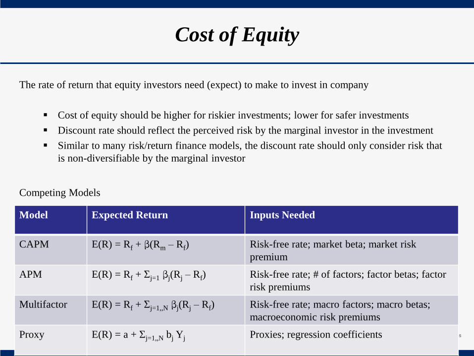
The rate of return that equity investors need (expect) to make to invest in company
Cost of equity should be higher for riskier investments; lower for safer investments
Discount rate should reflect the perceived risk by the marginal investor in the investment
Similar to many risk/return finance models, the discount rate should only consider risk that
is non-diversifiable by the marginal investor
Competing Models
Model Expected Return Inputs Needed
CAPM E(R) = Rf + (Rm – Rf) Risk-free rate; market beta; market risk
premium
APM E(R) = Rf + j=1 j(Rj – Rf) Risk-free rate; # of factors; factor betas; factor
risk premiums
Multifactor E(R) = Rf + j=1,,N j(Rj – Rf) Risk-free rate; macro factors; macro betas;
macroeconomic risk premiums
Proxy E(R) = a + j=1,,N bj Yj Proxies; regression coefficients

CAPM: Cost of Equity
Cost of Equity = Risk-free Rate + Equity Beta * (Equity Risk Premium)
In practice…
Risk-free rates: usually use government security rates
Risk premium: usually use historical risk premiums
Beta: usually estimated by regressing stock returns against market returns
But wait… each of these practices suffers from serious limitations

Risk-free Rate
• On a risk-free asset, the actual return is equal to the expected return.
NO variance around the expected return
• For an investment to be risk-free, it has to have
No default risk
No reinvestment risk
Considerations:
Time horizon
Not all government securities are risk-free (HINT: remove default risk)
US Treasury Rates
Local Currency Government Bond Rates
Country CDS spreads
Risk-free Rate
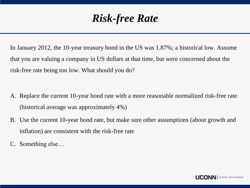
In January 2012, the 10-year treasury bond in the US was 1.87%; a historical low. Assume
that you are valuing a company in US dollars at that time, but were concerned about the
risk-free rate being too low. What should you do?
A. Replace the current 10-year bond rate with a more reasonable normalized risk-free rate
(historical average was approximately 4%)
B. Use the current 10-year bond rate, but make sure other assumptions (about growth and
inflation) are consistent with the risk-free rate
C. Something else…

Historical Risk Premium
• The historical risk premium is the difference between the realized annual return from investing in
stocks and the realized annual return from investing in a riskless security over a past time period.
Premiums are sensitive to:
• Time horizon (how far back should you go?)
• Rates (T-bill or T-bond?)
• Assumptions (Arithmetic average or geometric average?)
Some problems with using historical premiums:
Noisy estimates
Survivorship bias
Assume that next year turns out to be a terrible year for stocks. What would happen to the historical
risk premium if that occurs?
A. Go up
B. Go down
Country Risk Premium
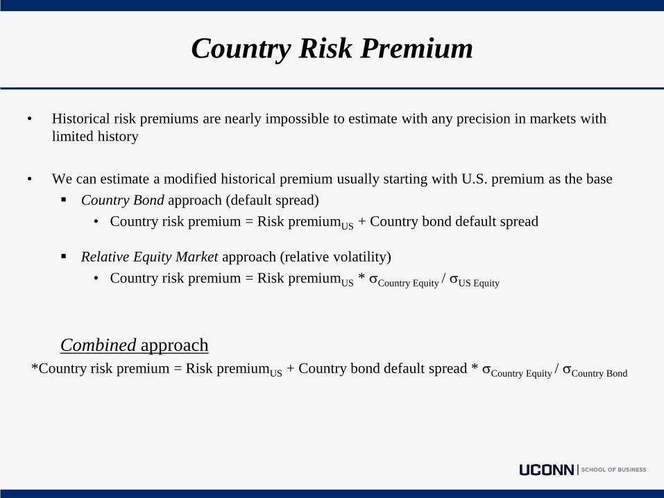
• Historical risk premiums are nearly impossible to estimate with any precision in markets with
limited history
• We can estimate a modified historical premium usually starting with U.S. premium as the base
Country Bond approach (default spread)
• Country risk premium = Risk premiumUS + Country bond default spread
Relative Equity Market approach (relative volatility)
• Country risk premium = Risk premiumUS * Country Equity / US Equity
Combined approach
*Country risk premium = Risk premiumUS + Country bond default spread * Country Equity / Country Bond

Country Risk Premium
Approach 1: Assume that every company in the country is equally exposed to country risk
E(Return) = Risk-free Rate + CRP + Beta (Mature ERP)
Approach 2: Assume that a company’s exposure to country risk is similar to its exposure to other
market risk
E(Return) = Risk-free Rate + Beta (Mature ERP + CRP)
Approach 3: Treat country risk as a separate risk factor and allow firms to have different exposures to
country risk
E(Return) = Risk-free Rate + Mature ERP + (CRP)
= % of revenues domesticallyfirm / % of revenues domesticallyavg firm
ERP = Equity risk premium
CRP = Country risk premium

Country Risk Premium: Example
Consider the following information for Firm B:
Beta: 1.07
US Risk-free rate: 4%
US market risk premium: 5%
Country risk premium (Portugal): 7.89%
Firm B gets 3% of its revenues from Portugal; 97% from US
Average Portuguese firm gets 11% of revenues from Portugal
Estimate Cost of Equity for Firm B.
E(Return) = 4% + 1.07 (5%) + 7.89% = 17.24% Approach 1
E(Return) = 4% + 1.07 (5%) + (0.03*7.89% + 0.97*0.0%) = 9.59% Approach 1a
E(Return) = 4% + 1.07 (5% + 7.89% )= 17.79% Approach 2
E(Return) = 4% + 1.07 (5% + (0.03*7.89% + 0.97*0.0%)) = 9.60% Approach 2a
E(Return) = 4% + 1.07 (5%) + 0.27*7.89% = 11.48% Approach 3

Estimating Beta
• Standard procedure: regress stock returns against market returns: Rj = a + b Rm
• The slope of the regression corresponds to the beta of the stock, thus measures the riskiness of the stock.
• Considerations:
Length of estimation period
Return interval
Benchmark
Economic conditions
• Some problems with this approach
High standard error
Reflects historical business mix; not current mix
Reflects firms’ average leverage over the period; not current capital structure
• Possible solutions
Modify regression beta by changing the index or by using company fundamentals
Estimate beta using std. dev. of stock returns or adjusted earnings
Estimate beta using bottom-up approach (business mix; financial leverage)
Use alternate (non-regression-based) measure of market risk

Estimating Beta: Yahoo! Finance example
Here is how you can calculate the beta provided by Yahoo! Finance:
1. Download monthly prices for your company and S&P 500 (Ticker: ^GSPC) for the past three
years (February 2012 – January 2015) from Yahoo! Finance (put them both in the same Excel
spreadsheet)
2. Calculate the monthly returns for your company and S&P 500 (use the Adjusted Close price and
use a simple return calculation (this month/last month – 1))
3. Use the ‘slope’ function to calculate Beta (use the monthly returns from your company for the
“known y’s” and the monthly returns from S&P 500 as the “known x’s”)
*You can also run a regression in Excel to get beta, along with other data. In Excel, go to options –
Add-Ins – Analysis ToolPak and click Go. Then in the Data tab, the button for Data Analysis should
appear. Click Data Analysis, and scroll to Regression. Input the same X and Y ranges, and you
should get the same beta coefficient as before.
** Alternatively, you can use the COVARIANCE.S formula and the VAR formula in Excel to
compute beta using the returns data for your company and a market index. Many resources are
available online to refresh your skills with using covariance and variance formulas.

Determinants of Beta
Product or Service
A firm’s beta depends upon the sensitivity of the demand for its products and services and
of its costs to macroeconomic factors that affect the overall market.
• Cyclical companies have higher betas than non-cyclical firms
• Firms which sell more discretionary products will have higher betas than firms that sell
less discretionary products
Operating Leverage
The greater the proportion of fixed costs in the cost structure of a business, the higher the
beta; because higher fixed costs increase your exposure to all risk (including market risk).
Financial Leverage
The more debt a firm takes on, the higher the beta; because debt creates a fixed cost (interest
expense) that increases exposure to market risk.
Equity Betas and Leverage
• Equity beta can be written as a function of the unlevered beta and the D/E ratio
L = u (1+((1-t)D/E))
where
L = Levered or Equity beta
u = Unlevered beta (Asset beta)
t = Corporate marginal tax rate
D = Market value of debt
E = Market value of equity

Bottom-up Beta
• The bottom up beta can be estimated by :
Taking a weighted (by sales or operating income) average of the unlevered betas of the
different businesses a firm is in.
j = 1,,k j [Operating Incomej / Operating IncomeFirm ]
(The unlevered beta of a business can be estimated by looking at other firms in the same business)
Lever up using the firm’s debt/equity ratio
levered = unlevered[1+ (1- tax rate) (Current Debt/Equity Ratio)]
• The bottom up beta will give you a better estimate of the true beta because:
It has lower standard error (SEaverage = SEfirm / √n)
It reflects the firm’s current business mix and financial leverage
It can be estimated for divisions and private firms.

Unlevering Beta: Example
Consider the following information for Firm A:
• Regression beta: 0.95
• Average D/E during regression period: 24.64%
• Marginal tax rate: 38%
Compute Firm A’s unlevered beta.
Unlevered A = Levered A / [1 + (1-tax rate)(Average D/E)]
Unlevered A = 0.95 / [1 + (1-38%)(24.64%)]
Unlevered A = 0.8241

Bottom-up Beta: Example
Consider the following information for Firm A:
Assume:
• marginal tax rate is 35%
• MV Equity = $33,401
• MV Debt = $8,143
Compute Firm A’s Levered Beta.
Unlevered A = (0.91 * 70.39%) + (0.80 * 29.61%) = 0.88
Market D/E ratio = 8,143 / 33,401 = 24.38%
Levered A = 0.88 * (1 + (1-.35) * (24.38%)) = 1.02
Segment Division Revenues EV / Sales Unlevered Beta Segment Weight
Media 12,411.72 2.43 0.91 70.39%
Consumer Products 6,784.76 1.87 0.80 29.61%
Cost of Debt
The cost of debt is the current rate at which you can borrow. It reflects both the default risk and the
level of interest rates in the market.
• Two widely used approaches to estimating cost of debt are:
Use the yield to maturity on a straight bond outstanding from the firm.
• Limitation: very few firms have long term straight bonds that are liquid and widely
traded
Use the rating for the firm and estimate a default spread based upon the rating.
• Limitation: different bonds from the same firm can have different ratings.
Hint: If a firm is not rated (or has multiple ratings), estimate a synthetic rating and the cost of debt
based upon that rating.
Synthetic rating could be estimated using the interest coverage ratio (EBIT / Interest Expenses);
but the relative importance of these ratios in estimating default risk has changed over time
Credit Ratings
Moody's states that “the purpose of ratings is to provide investors with a simple system of gradation by which future
relative creditworthiness of securities may be gauged.”
S&P states “A credit rating is Standard & Poor's opinion on the general creditworthiness of an obligor, or the
creditworthiness of an obligor with respect to a particular debt security or other financial obligation. Over the
years credit ratings have achieved wide investor acceptance as convenient tools for differentiating credit quality.”
Moody’s Ratings
Aaa Obligations rated Aaa are judged to be of the highest quality, with minimal credit risk.
Aa Obligations rated Aa are judged to be of high quality and are subject to very low credit risk.
A Obligations rated A are considered upper-medium grade and are subject to low credit risk.
Baa Obligations rated Baa are subject to moderate credit risk. They are considered medium-grade and as
such may possess certain speculative characteristics.
Ba Obligations rated Ba are judged to have speculative elements and are subject to substantial credit risk.
B Obligations rated B are considered speculative and are subject to high credit risk.
Caa Obligations rated Caa are judged to be of poor standing and are subject to very high credit risk.
Ca Obligations rated Ca are highly speculative and are likely in, or very near, default, with some prospect
of recovery of principal and interest.
C Obligations rated C are the lowest rated class of bonds and are typically in default, with little prospect
for recovery of principal or interest

Weighted Average Cost of Capital (WACC)
The weights used to compute the cost of capital should be the market value weights for debt and
equity.
• As a general rule, the debt that you should subtract from firm value to arrive at the value of
equity should be the same debt that you used to compute the cost of capital.
Example
• Cost of Equity = 5.10% + 0.96 (4%+1.59%) = 10.47%
• Cost of Debt = 5.10% + 0.75% +0.95%= 6.80%
Market Value of Equity = $739,217 (78.7%)
Market Value of Debt = $199,766 (21.3 %)
Cost of Capital = 10.47 % (.787) + 6.80% (1- .2449) (0.213)) = 9.33 %
Cost of Capital recap
Cost of Capital =
Cost of Equity (Equity/(Debt + Equity)) + Cost of Borrowing (1-t) (Debt/(Debt + Equity))
Cost of Equity= Risk-free Rate + Beta (Mature Market Premium) + Lambda (Country Risk Premium)
Cost of Debt = Pre-tax Cost of Debt * (1 – marginal tax rate)
Risk-free Rate: usually use government bond rates (adjusted for default risk)
Beta: can use slope from regression of historical prices (easy, but problematic); or could estimate bottom-up beta
Mature Market premium: US is typically considered a mature market; be careful relying on historical premiums
Lambda: sensitivity of firms’ revenues to country risk (% of revenues domesticallyfirm/ % of revenues domesticallyavgfirm)
Country Risk premium: Additional premium (beyond the mature market) added for country-specific risk
Pre-tax Cost of Debt: Risk-free Rate + Company Default Spread + Lambda(Country Default Spread)
Marginal tax rate: amount of tax paid on additional dollar of income (do NOT simply rely on effective tax rates)
Prospect Theory
Experiment 1:
Would you rather receive:
A. An 80% chance to win $4,000, 20% win nothing; or
B. A certain gain of $3,000
Experiment 2:
Would you rather receive:
C. An 80% chance to lose $4,000, 20% to lose nothing; or
D. A certain loss of $3,000
Experimental economists have often found most of people choose B over A; and C over D.
Implications:
• People seem to respond to perceived gains or losses rather than to their hypothetical final wealth
positions (as would be assumed by expected utility theory).
• There is a diminishing marginal sensitivity to changes, regardless of the sign of the changes; and
• Loss looms larger than gains.

Earnings Management
What is it?
“A gray area where the accounting is being perverted; where managers are cutting corners; and,
where earnings reports reflect the desires of management rather than the underlying financial
performance of the company.”
- Arthur Levitt, The “Numbers Game”, from speech given on September 28, 1998
“Earnings management occurs when managers use judgment in financial reporting and in
structuring transactions to alter financial reports to either mislead some stakeholders about the
underlying economic performance of the company to influence contractual outcomes that depend on
reported accounting numbers”
Healy and Wahlen, 1999
In many cases, earnings management is used to increase income in the current year at the expense of
income in future years; however, earnings management can also be used to decrease current earnings
in order to increase income in the future.
Income smoothing (sometimes considered a form of earnings management) is often defined as the
planned timing of revenues, expenses, gains and losses to smooth out bumps in earnings.

Earnings Management: Public Perception
• Earnings management has a negative effect on the quality of earnings if it distorts the
information in a way that it less useful for predicting future cash flows. The term ‘earnings
quality’ refers to the credibility of the earnings number reported. Earnings management reduces
the reliability of income.
• The investing public does not necessarily view minor earnings management as unethical, but in
fact as a common and necessary practice in the everyday business world. Oftentimes, it is only
when the impact of earnings management is great enough to adversely affect investment
decisions that earnings management is viewed negatively.
What is Earnings Quality?
• Earnings quality is largely contextual. Its definition often depends on the user
Standard setters
Auditors
Compensation committees
Debt-holders
Investors
Financial analysts
Most would agree that fraudulent reporting is of low quality

What is Earnings Quality?
Financial analyst objectives
Forecast earnings
Make stock recommendations
• Thus, earnings are of higher quality if they:
Are more predictable
• High persistence
• Few transitory components
• Less volatile
Are easier to forecast
Map into intrinsic value
• Current stock price
• Actual future cash flows
• Residual income

Earnings Quality
What affects earnings predictability across firms?
Stage of firms’ life cycle (steady state vs. growing / declining)
• Sources of competition for growing firms
• Transitory components and losses for declining firms
• Financial statement analysis
Quality of management’s forecasts and estimates
Accounting standards
Voluntary disclosures
Earnings Quality
Many companies struggle to meet earnings expectations. As a result, companies often engage in
activities that may reduce the quality of their earnings. Some of these activities are:
Adopting less conservative accounting practices
One-time transactions
Impairment charges
Restructuring charges
Pulling future earnings into present period
Recognizing past profits in current period
Adopting new accounting standards
‘Managing’ discretionary expenses
Under-reserving for the future (i.e., bad debt expense, warranty obligations)
Increased reliance on ‘non-core’ earnings
Lease structuring
M&A activity with inadequate disclosure
Rapid investment write-offs
Increased leverage
Earnings Quality
Many companies struggle to meet earnings expectations. As a result, companies often engage in activities that may
reduce the quality of their earnings. Some factors that may prompt managers to take actions that reduce the quality
of their earnings include:
External pressures
Equity market expectations
Analyst forecasts
Debt markets and contractual obligations
Competition
Emerging financial instruments
Limited attention / market ‘inefficiencies’
Internal factors
Potential mergers/acquisitions
Management compensation
Planning and budgets
Unlawful transactions
Personal factors
Bonuses
Promotions and job retention
Low regard for auditors
Leases
The principal advantages perceived by companies who enter into leases are:
Off-balance sheet financing: Firms are able to use assets in their business without showing
the related debt. Firms improve the utilization of their assets via leasing since they can add
capacity, as needed, a lot more easily by leasing rather than committing to own the assets.
No interest expense or depreciation: However, both of these are part of the “lease expense”
account that does run through the income statement.
Avoid certain risks of ownership: examples include technological obsolescence, physical
deterioration, etc. If one of these situations arises, the firm may terminate the lease, although
there may be a penalty involved.
Tax advantages: If the lessee is in a lower marginal tax bracket than the lessor, leasing is
advantageous to both parties. The lessor can take advantage of any accelerated depreciation
tax shields available to them and some of this benefit is usually passed on to the lessee in
reduced lease payments.

Leases
Operating leases are leases that fail all of the following four tests under Financial Accounting
Standard (FAS) No.13 (or more recent updates) and, therefore qualify for off-balance sheet
treatment:
• The lease transfers ownership of the asset to the lessee by the end of the lease term.
• The lease contains an option to purchase the leased property at a bargain price.
• The lease term is equal to or greater than 75% of the estimated useful life of the leased asset.
• The PV of the lease and other minimum lease payments equals or exceeds 90 percent of the fair
value of the leased asset.

Operating Leases
Operating income is often a key input in firm valuation models
Implicit assumption: operating expenses include only those expenses
designed to create revenue in the current period
Most analysts will capitalize operating leases back into the company’s financial
statements to get a more proper view of their true debt and related expenses – in
other words, as if the company bought the asset outright and took on debt to
finance it.

Capitalizing Leases
1. Take current year and next five years’ cash payments as given
2. Divide the ‘Thereafter’ amount by the year+5 amount to get the approximate number of years
left (at the year+5 level) of lease payments. Then, put that number of years (rounded up) worth of
constant payments into your PV computation.
3. Compute present value of lease payments (use the company’s approximate long-term borrowing
rate, matching the long-term nature of its assets).
4. Adjust financials
a) Add PV of lease payments to the long term asset section of the balance sheet as “Assets
Under Capitalized Leases”, and a like amount to the liabilities section as “Capitalized Lease
Obligations” (this now assumes that the company had purchased the assets with borrowed
money).
b) Reverse the existing Lease Expense entry currently on the books (note: lease expense may
be included in another expense category, such as SG&A, etc.)
c) Calculate the implied interest expense portion of the current year’s payment.
d) Use present value of lease payments to compute depreciation expense (straight-line method
is acceptable)
e) Adjusted NI = NI + Operating Lease Expenses – Imputed Interest Expense - Depreciation
Capitalizing Operating Leases
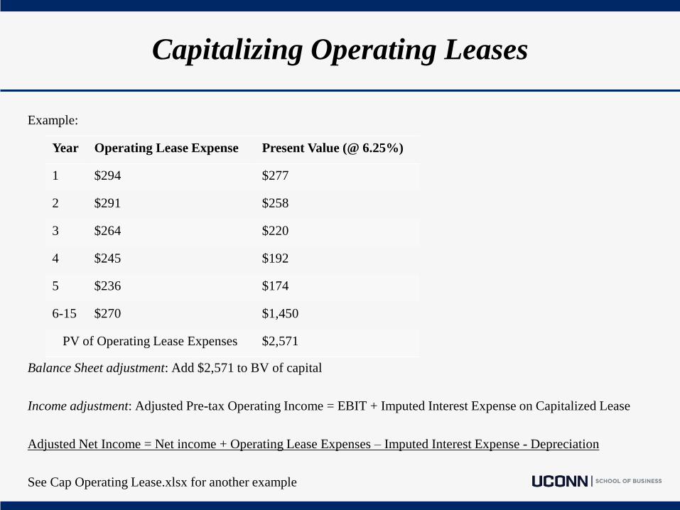
Example:
Balance Sheet adjustment: Add $2,571 to BV of capital
Income adjustment: Adjusted Pre-tax Operating Income = EBIT + Imputed Interest Expense on Capitalized Lease
Adjusted Net Income = Net income + Operating Lease Expenses – Imputed Interest Expense - Depreciation
See Cap Operating Lease.xlsx for another example
Year Operating Lease Expense Present Value (@ 6.25%)
1 $294 $277
2 $291 $258
3 $264 $220
4 $245 $192
5 $236 $174
6-15 $270 $1,450
PV of Operating Lease Expenses $2,571

Operating vs. Capital Leases
Operating Lease effect on net income (similar to interest payments)
After-tax Effect of Lease on Net Income = Lease Payment (1-t)
Capital Lease Example:
5-year capital lease
Lease payments $1 million / year
Firm’s cost of debt: 10%
Present Value of Lease Payments = $1m (PV of Annuity, 10%, 5 years) = $3,790,787
Year Lease
Payment
Imputed
Interest Expense Reduction in Lease Liability Lease Liability Depreciation Total Tax Deduction
1 $1,000,000 $379,079 $620,921 $3,169,865 $758,157 $1,137,236
2 $1,000,000 $316,987 $683,013 $2,486,852 $758,157 $1,075,144
3 $1,000,000 $248,685 $751,315 $1,735,537 $758,157 $1,006,843
4 $1,000,000 $173,554 $826,446 $909,091 $758,157 $931,711
5 $1,000,000 $90,909 $909,091 $0 $758,157 $849,066

Operating vs. Capital Leases
In general, when a lease is treated as an operating lease rather than a capital lease:
Operating income is lowered (effect on net income depends on lease horizon)
Debt and capital is understated
Return on equity (RoE) and return on capital (RoC) is higher

Pensions
Defined Benefit vs. Defined Contribution
In a Defined Benefit pension plan an employer or sponsor promises a
specified monthly benefit on retirement that is formulaically predetermined based
on the employee's earnings history, tenure of service and age. The employer
bears the risk of funding the plan. ERISA funding rules require plans to maintain
a pool of assets covering a portion of the projected benefit obligations.
Defined Contribution plans shift risk to the employees. Firms are not required to
set aside a pool of assets to meet future retirement benefits. Employees maintain
their own account balances.
Should earnings be adjusted to account for these plans?
See http://www.danemott.com/john-deere-adjust-pension-opebs/ for a discussion and detailed
analysis of how one research firm adjusts financial statements for defined benefit pension plans and
OPEBs. Also see DE pension adjustment.xlsx for additional guidance.

Research & Development expense
US GAAP requires R&D to be expensed in the current period, even though it is
designed to generate future growth.
Perhaps, it is more logical to treat it as capital expenditures

Capitalizing Research & Development expense
1. Determine the amortizable life of the R&D asset.
This depends on many factors, such as the length of time it takes to get a patent
approved, and the duration of a patent. You can look in the 10-K to look at some
of the assumptions your firm makes about the amortizable life of intangible assets,
and/or if they talk about the length of time it takes to get a patent.
2. Collect past R&D expense for each year, starting from the time that you first decide to
amortize the asset.
If you assume an amortizable life of ten years, you should get R&D expense
starting from ten years before, including the current year.
3. Sum the unamortized portion of R&D expense.
To make it simple, assume a straight line amortizable life for the asset. So, for the
R&D expense in 2005, only 1/10 would still be unamortized in 2014; only 2/10 of
2006 R&D expense would still be unamortized in 2014; and so on…
Capitalizing Research & Development expense
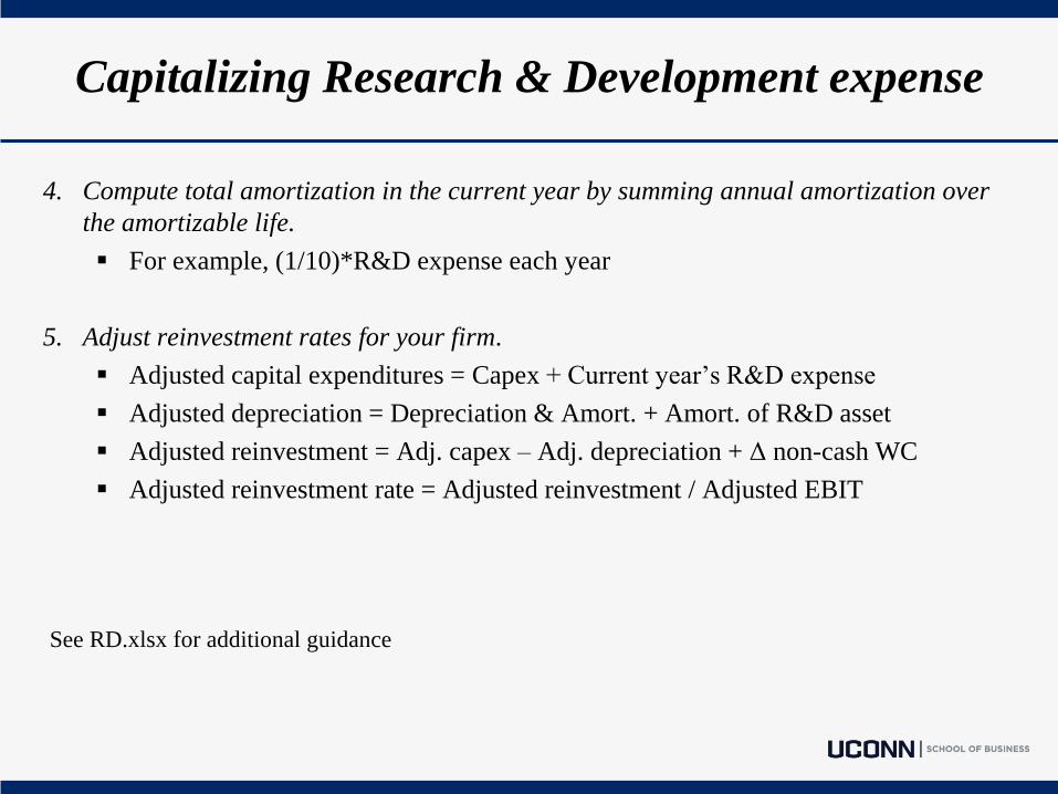
4. Compute total amortization in the current year by summing annual amortization over
the amortizable life.
For example, (1/10)*R&D expense each year
5. Adjust reinvestment rates for your firm.
Adjusted capital expenditures = Capex + Current year’s R&D expense
Adjusted depreciation = Depreciation & Amort. + Amort. of R&D asset
Adjusted reinvestment = Adj. capex – Adj. depreciation + Δ non-cash WC
Adjusted reinvestment rate = Adjusted reinvestment / Adjusted EBIT
See RD.xlsx for additional guidance
Capitalizing Research & Development expense
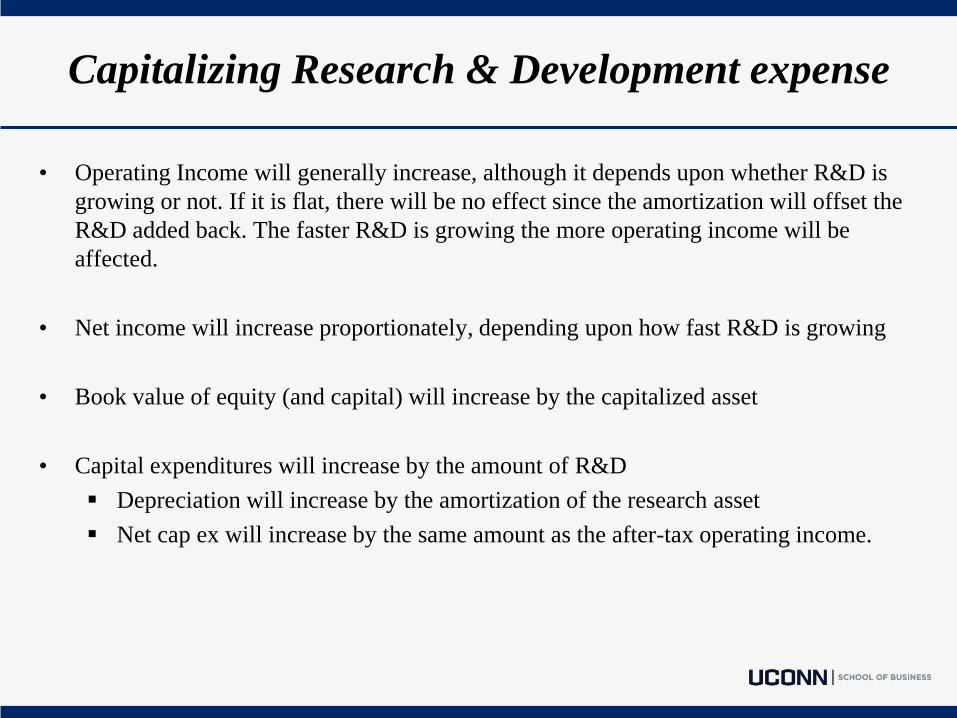
• Operating Income will generally increase, although it depends upon whether R&D is
growing or not. If it is flat, there will be no effect since the amortization will offset the
R&D added back. The faster R&D is growing the more operating income will be
affected.
• Net income will increase proportionately, depending upon how fast R&D is growing
• Book value of equity (and capital) will increase by the capitalized asset
• Capital expenditures will increase by the amount of R&D
Depreciation will increase by the amortization of the research asset
Net cap ex will increase by the same amount as the after-tax operating income.

Other Earnings Adjustment Concerns
• Debt Valuation Adjustments (FAS 159)
JP Morgan: $1.9 billion gain
• Gain allowed JP to ‘beat’ analyst forecasts
• Stock price still dropped by almost 5%
Bank of America: $6.2 billion gain
Morgan Stanley: $5.1 billion gain
Goldman Sachs: $450 million gain
Citigroup $1.7 billion gain
Merrill Lynch: $4 billion gain
• Excess Cash
• Discontinued Operations
• One-time gains / losses
• Changes in reserves

Net Capital expenditures
• Net capital expenditures = capital expenditures - depreciation
Depreciation may be considered a cash inflow that pays for some, or perhaps all,
capital expenditures.
• In general, net capex = f(growth, E(growth))
High growth firms are expected to have higher net capex than low growth firms.
• Net capex includes:
R&D expenses (after being capitalized)
• Adj. net capex = Net capex + current year’s R&D expense – Amort. of Research Asset
Acquisitions of other firms
• Adj. net capex = Net capex + Acquisitions of other firms - Amort. of such acquisitions
Note: firms do not necessarily do acquisition every year, therefore a normalized acquisition measure
should by employed. Acquisitions may be found in the Cash Flow statement.

Net Capital expenditures
Example (2014 Cisco Systems, Inc.)
Cap Expenditures (from statement of CF) $1,275
- Depreciation (from statement of CF) (2,432)
Net Cap Ex (1,157)
+ R & D expense (10-k) 6,294
- Amortization of R&D (own calculation) (1,818)
+ Acquisitions 3,181
Adjusted Net Capital Expenditures 6,500
Working Capital investments
• From an accounting perspective:
Working capital = current assets - current liabilities
• Current assets include inventory, cash, A/R, etc.
• Current liabilities include A/P, short-term debt, LT debt due within one year,
etc.
• From an economic (cash flow) perspective:
Working Capital = non-cash current assets - non-debt current liabilities
Note: Any investment of working capital ties up cash. Therefore, increases
(decreases) in working capital will reduce (increase) cash flows in that period.
When forecasting future growth, it is important to estimate the effects of such
growth on working capital needs, and to build these effects into forecasted cash
flows.

Working Capital investments
Why back out cash (and other marketable securities)?
The instruments are typically invested by firms in treasury bills, short term government
securities or commercial paper.
While the return on these investments may be lower than what the firm may make on its real
investments, they represent a fair return for riskless investments.
Unlike inventory, accounts receivable and other current assets, cash then earns a fair return
and should not be included in measures of working capital.
Are there exceptions to this rule? When valuing a firm that has to maintain a large cash
balance for day-to-day operations or a firm that operates in a market in a poorly developed
banking system, you could consider the cash needed for operations as a part of working
capital.
Why back out all interest bearing debt, short term debt, and the portion of long term debt that is due
in the current period from the current liabilities?
This debt will be considered when computing cost of capital and it would be inappropriate
to count it twice.
Working Capital investments
General principles
• Volatility
Changes in non-cash working capital from year to year tend to be volatile. A far
better forecast of future non-cash working capital needs can be estimated by
looking at non-cash working capital as a proportion of revenues
• Dealing with negative working capital
Some firms have negative non-cash working capital. While these firms certainly
can generate positive near-term future cash flows, assuming negative non-cash
working capital into perpetuity is not feasible. A better approach (when dealing
with firms with negative non-cash WC) would be to set non-cash working capital
needs to zero.

Dividends and Cash Flow to Equity
• Strictly speaking, the only cash flow investors receive from an equity investment in a publicly
traded firm is the dividend that will be paid on the stock.
• Managers set actual dividends paid
distributed dividends may be much lower than the potential dividends
managers are conservative and try to smooth out dividends
managers often hold on to cash to meet unforeseen future contingencies and investment
opportunities
Note: when actual dividends are less than potential dividends, using a model that focuses
only on dividends will understate the true value of equity in a firm.
Dividends and Cash Flow to Equity
What are potential dividends?
• The potential dividends of a firm are the cash flows left over after the firm has made any
“investments” it needs to make to create future growth and net debt repayments
Are earnings a good proxy for potential dividends?
• NO!!!
• Some analysts assume that the earnings of a firm represent its potential dividends. This cannot be
true for several reasons:
Earnings are NOT cash flows! Earnings contains both non-cash revenues and expenses
Even if earnings were cash flows, a firm that paid its earnings out as dividends would not be
investing in new assets and thus could not grow
Valuation models, where earnings are discounted back to the present, will misestimate the
value of the equity in the firm
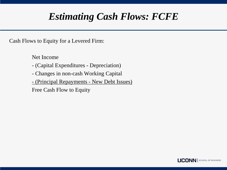
Estimating Cash Flows: FCFE
Cash Flows to Equity for a Levered Firm:
Net Income
- (Capital Expenditures - Depreciation)
- Changes in non-cash Working Capital
- (Principal Repayments - New Debt Issues)
Free Cash Flow to Equity
Estimating Cash Flows: FCFE
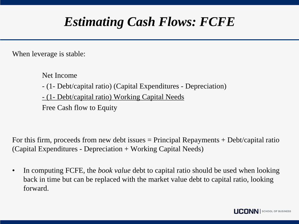
When leverage is stable:
Net Income
- (1- Debt/capital ratio) (Capital Expenditures - Depreciation)
- (1- Debt/capital ratio) Working Capital Needs
Free Cash flow to Equity
For this firm, proceeds from new debt issues = Principal Repayments + Debt/capital ratio
(Capital Expenditures - Depreciation + Working Capital Needs)
• In computing FCFE, the book value debt to capital ratio should be used when looking
back in time but can be replaced with the market value debt to capital ratio, looking
forward.

Estimating Cash Flows: FCFE
Example:
Consider the following per share information for TGI, Inc. for 2013:
EPS: $4.75
Investment in fixed capital: $1.20
Depreciation: $0.65
Investment in WC: $0.95
TGI is currently operating at target debt/capital ratio of 30%. Shareholders require a 14%
return on investment. Expected growth rate is 6%
What is the TGI’s FCFE?
$4.75
- (1- 30%) (1.20 – 0.65)
- (1- 30%) (0.95)
$3.70
What is the value of TGI’s stock?
Equity value per share = ($3.70 * 1.06) / (0.14 – 0.06)
Equity value per share = $65.37

Analyzing Cash Flow information
Cash flow from operations
• How strong is the firm’s internal cash flow generation? Is cash flow from operations positive? If it is negative,
why? Is it because the company is growing? Are operations unprofitable? Are there too many inefficiencies?
Short-term liquidity
• Does the company have the ability to meet its short-term financial obligations, such as interest payments, from
its operating cash flow? Can it continue to meet these obligations without reducing its operating flexibility?
Reinvestment
• How much cash did the company invest in growth? Are these investments consistent with its business strategy?
Did the company use internal cash flow to finance growth, or did it rely on external financing? Does the
company have excess cash flow after making capital investments? What plans does management have to
deploy free cash flow?
Dividends
• Did the company pay dividends from internal free cash flow? If the company had to rely on external financing
to pay dividends, is the company’s dividend policy sustainable?
Financing
• What type of external financing does the company rely on (i.e., equity, short-term debt, long-term debt)?
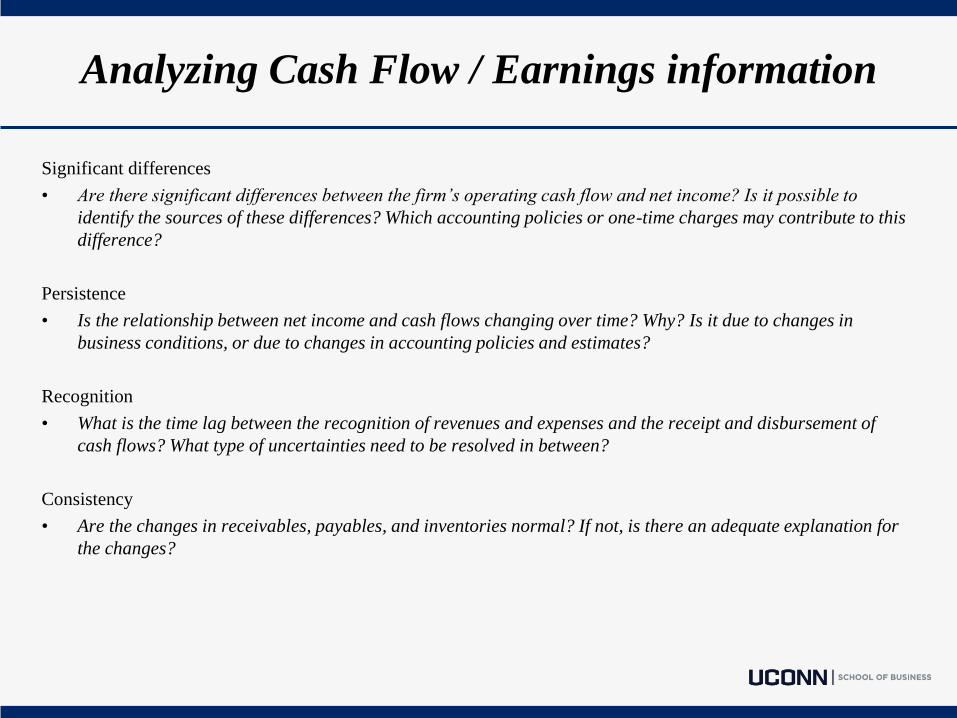
Analyzing Cash Flow / Earnings information
Significant differences
• Are there significant differences between the firm’s operating cash flow and net income? Is it possible to
identify the sources of these differences? Which accounting policies or one-time charges may contribute to this
difference?
Persistence
• Is the relationship between net income and cash flows changing over time? Why? Is it due to changes in
business conditions, or due to changes in accounting policies and estimates?
Recognition
• What is the time lag between the recognition of revenues and expenses and the receipt and disbursement of
cash flows? What type of uncertainties need to be resolved in between?
Consistency
• Are the changes in receivables, payables, and inventories normal? If not, is there an adequate explanation for
the changes?

Estimating Earnings Growth
1) Historical growth in EPS (typically a good starting point)
Regression analysis
Arithmetic vs. Geometric averages
Other Considerations:
Time period
Negative earnings in current period
Changes in firm size, capital structure, life cycle, etc.
Example:
Revenues Change % EBITDA Change % EBIT Change %
20x1 8,945 1,152 612
20x2 9,574 7.03% 1,352 17.36% 688 12.42%
20x3 10,310 7.69% 998 -26.18% 462 -32.85%
20x4 13,554 31.46% 1,012 1.40% 460 -0.43%
20x5 12,976 -4.26% 787 -22.23% 229 -50.22%
20x6 13,228 1.94% 1,480 88.06% 719 213.97%
Arithmetic Avg. 8.77% 11.68% 28.58%
Geometric Avg. 8.14% 5.14% 3.28%
Std. Dev. 13.56% 46.25% 106.60%
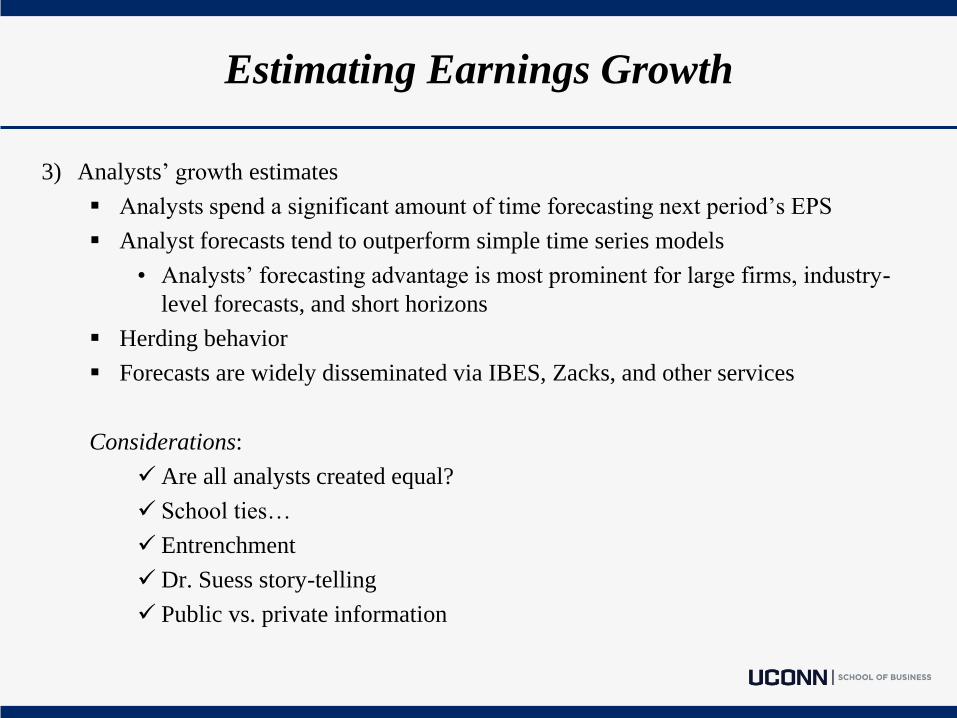
Estimating Earnings Growth
3) Analysts’ growth estimates
Analysts spend a significant amount of time forecasting next period’s EPS
Analyst forecasts tend to outperform simple time series models
• Analysts’ forecasting advantage is most prominent for large firms, industry-
level forecasts, and short horizons
Herding behavior
Forecasts are widely disseminated via IBES, Zacks, and other services
Considerations:
Are all analysts created equal?
School ties…
Entrenchment
Dr. Suess story-telling
Public vs. private information

Estimating Earnings Growth
2) Fundamental analysis
Reinvestment (is the firm investing in new projects?)
• Reinvestment rate (or retention ratio) = Retained earnings / Current earnings
Expected ROI
• ROI (or ROE) = Net income / Book value of equity
Simple example:
Investment in
Current Projects
x Current ROI = Current
Earnings
$100 x 12% = $12
Investment in
Current Projects
x Current ROI + Investment in
new projects
x ROI on new
projects
= Next period’s
earnings
$100 x 12% + $50 x 12% = $18

Estimating Earnings Growth
Growth Rate:
Investment in Current Projects x Δ ROI + New Projects x ROI = Δ Earnings
Investment in Current Projects * Current ROI Current Earnings
Using prior example:
$100 x 0% + $50 x 12% = $6 = 50%
$100 x 12% $12
Now assume that expansion into China will improve ROI to 13%. What is the new
expected growth rate?
$100 x 1% + $50 x 13% = $7.50 = 62.50%
$100 x 12% $12

Estimating Earnings Growth
When looking at growth in operating income:
Reinvestment Rate = (Net CapEx + Δ WC) / EBIT(1-t)
Return on Investment = ROC = EBIT(1-t) / (BV of debt + BV of equity)
gEBIT = (Net CapEx + Δ WC) / EBIT(1-t) * ROC = Reinvestment Rate * ROC
Note: For a given growth rate, firms’ net capex needs should be inversely proportional to
the quality of its investments.

Estimating Earnings Growth
ROE and leverage:
ROE = Return on capital + Debt/Equity (Return on capital – After-tax cost of debt)
Return on capital = EBITt (1-tax rate) / BV of capitalt-1
BV of capital = BV of debt + BV of equity
When looking at growth in net income:
Expected GrowthNet Income = Equity Reinvestment Rate * ROE
Equity Reinvestment Rate = (Net CapEx + Δ WC) (1 - Debt Ratio)/ Net Income
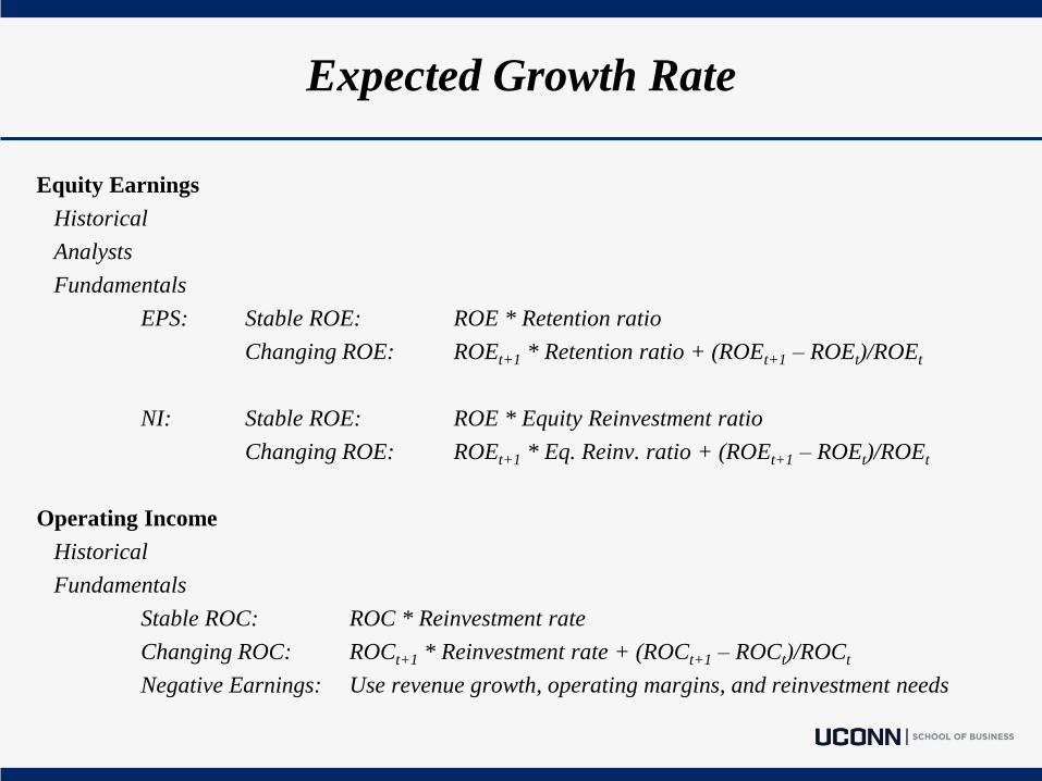
Expected Growth Rate
Equity Earnings
Historical
Analysts
Fundamentals
EPS: Stable ROE: ROE * Retention ratio
Changing ROE: ROEt+1 * Retention ratio + (ROEt+1 – ROEt)/ROEt
NI: Stable ROE: ROE * Equity Reinvestment ratio
Changing ROE: ROEt+1 * Eq. Reinv. ratio + (ROEt+1 – ROEt)/ROEt
Operating Income
Historical
Fundamentals
Stable ROC: ROC * Reinvestment rate
Changing ROC: ROCt+1 * Reinvestment rate + (ROCt+1 – ROCt)/ROCt
Negative Earnings: Use revenue growth, operating margins, and reinvestment needs

Estimating Earnings Growth
CA is still in its high-growth phase and has the following financial characteristics:
• Return on Assets = 25%
• Dividend Payout Ratio = 7%
• Debt/Equity Ratio = 10%
• Interest rate on Debt = 8.5%
• Corporate tax rate = 40%
It is expected to become a stable firm in ten years.
A. What is the expected growth rate (net income) for the high-growth phase?
0.93 (25% + 0.10 (25% - 8.50% * (1 - 0.4))) = 25.10%
Assume now that the industry averages for larger, more stable firms in the industry are as follows:
Industry Average: Return on Assets = 14%; Debt/Equity Ratio = 40%; Interest Rate on Debt = 7%;
Dividend Payout ratio = 50%
B. What would you expect the growth rate in the stable growth phase to be?
Expected Growth Rate = 0.5 (0.14 + 0.4 (0.14 - 0.07 * (1 - 0.4))) = 8.96%
Cash Valuation
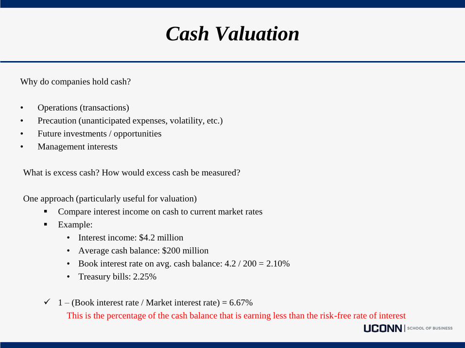
Why do companies hold cash?
• Operations (transactions)
• Precaution (unanticipated expenses, volatility, etc.)
• Future investments / opportunities
• Management interests
What is excess cash? How would excess cash be measured?
One approach (particularly useful for valuation)
Compare interest income on cash to current market rates
Example:
• Interest income: $4.2 million
• Average cash balance: $200 million
• Book interest rate on avg. cash balance: 4.2 / 200 = 2.10%
• Treasury bills: 2.25%
1 – (Book interest rate / Market interest rate) = 6.67%
This is the percentage of the cash balance that is earning less than the risk-free rate of interest

Cash Valuation
Cash is different from other assets:
No uncertainty surrounding its value; riskless
How do we value cash?
1) Estimate firm’s cash flows, as if firm had no cash
Adjusted EBIT = EBIT – Pre-tax interest income from cash and cash equivalents
Adjusted Net income = Net income – interest income (1-tax rate)
2) Estimate discount rate (assuming no cash)
Estimate cash balance as a percentage of firm value
Estimate weighted average unlevered beta
• Unlevered beta = Unlevered beta w/out cash (1-cash balance %) + 0 (cash balance %)
Compute new beta
• New beta = Unlevered beta w/out cash (1 + (1-tax rate) * (D/E)
Compute new cost of capital (use new beta for cost of equity)
3) Value firm (use adjusted cash flows and new discount rate)
Firm value = Value of assets + Cash
Value of Equity = Firm value – Value of debt

Cash Valuation – separate approach
Example:
MV Non-cash operating assets: $1,200 Cash: $ 200
Non-cash operating assets
Beta: 1.00
Expected return: $120 each year into perpetuity (no reinvestment, and no outstanding debt)
Cash is invested at risk-free rate: 4.5%
Market risk premium: 5.5%
Cost of equity for non-cash assets = 4.5% + 1 * 5.5% = 10%
Expected earnings from operating assets = $120
Value of non-cash assets = expected earnings / cost of equity for non-cash assets = 120 / 10% = $1,200
Value of equity = $1,200 + $200 = $1,400

Cash Valuation – consolidated approach
Example:
MV Non-cash operating assets: $1,200 Cash: $ 200
Non-cash operating assets
Beta: 1.00
Expected return: $120 each year into perpetuity (no reinvestment, and no outstanding debt)
Cash is invested at risk-free rate: 4.5%
Market risk premium: 5.5%
Beta = Betanon-cash * 1-Cash balance % + Betacash * Cash balance %
Beta = 1.00 * (1200/1400) + 0 * (200/1400) = 0.8571
Cost of equity = 4.5% + 0.8571 * 5.5% = 9.21%
Expected earnings = NI from operating assets + interest income from cash
Expected earnings = 120 + 4.5% * 200 = $129
Value of Equity = FCFE / Cost of equity = 129 / .0921 = $1,400
Note: If FCFE was discounted
at 10%, we would have valued
firm at $1,290. The entire
$110 difference in value
would be attributable to
discounting cash:
(4.5%*200) / 10% = $90
$200 - $90 = $110

Relative Valuation
In relative valuation, the value of an asset is compared to the values assessed by the market for
similar or comparable assets.
Therefore, to do relative valuation:
we need to identify comparable assets and obtain market values for these assets
convert market values into standardized values (price multiples)
compare multiples for the asset being analyzed to comparable asset
Note: be sure to control for any differences between the firms that might affect the
multiple

Relative Valuation
Prices can be standardized using variables such as earnings, cash flows, book value, revenues, etc.
Earnings Multiples
• Price/Earnings Ratio (PE) and variants (PEG and Relative PE)
• Value/EBIT; Value/EBITDA; Value/Cash Flow
Book Value Multiples
• Price/Book Value (PBV)
• Value/ Book Value of Assets; Value/Replacement Cost (Tobin’s Q)
Revenues
• Price/Sales per Share (PS)
• Value/Sales
Industry Specific Variables (Price/kwh, Beer share of throat, etc.)

Steps to Relative Valuation
1) Define the multiple
In practice, the same multiple can be defined in different ways by different users. When
comparing and using multiples, it is critical that we understand how multiples have been
estimated. Consider the example presented regarding analyst recommendations.
2) Present descriptive statistics on multiple
Oftentimes, people using multiples are unaware of its cross sectional distribution. It is
difficult to look at a number, without knowledge of its underlying distribution, and pass
judgment on whether it is too high or low.
3) Analyze the multiple
We must understand the fundamentals that drive each multiple, and the nature of the
relationship between the multiple and each variable.
4) Apply the multiple
Defining the comparable universe and controlling for differences is far more difficult in
practice than it is in theory.

Potential Pitfalls in Relative Valuation
1) Are both numerator and denominator consistently measured?
2) What should we do with outliers?
3) What should we do when multiple cannot be estimated for certain firms? Could this lead to bias?
4) Has the multiple changed over time?
5) What are the fundamentals that drive the relationship embedded in the multiple? Is the
relationship linear?
6) What are ‘comparable’ firms? Should firms be matched on size, capital structure, risk, growth,
industry, cash flows, etc.?
Accrual Example
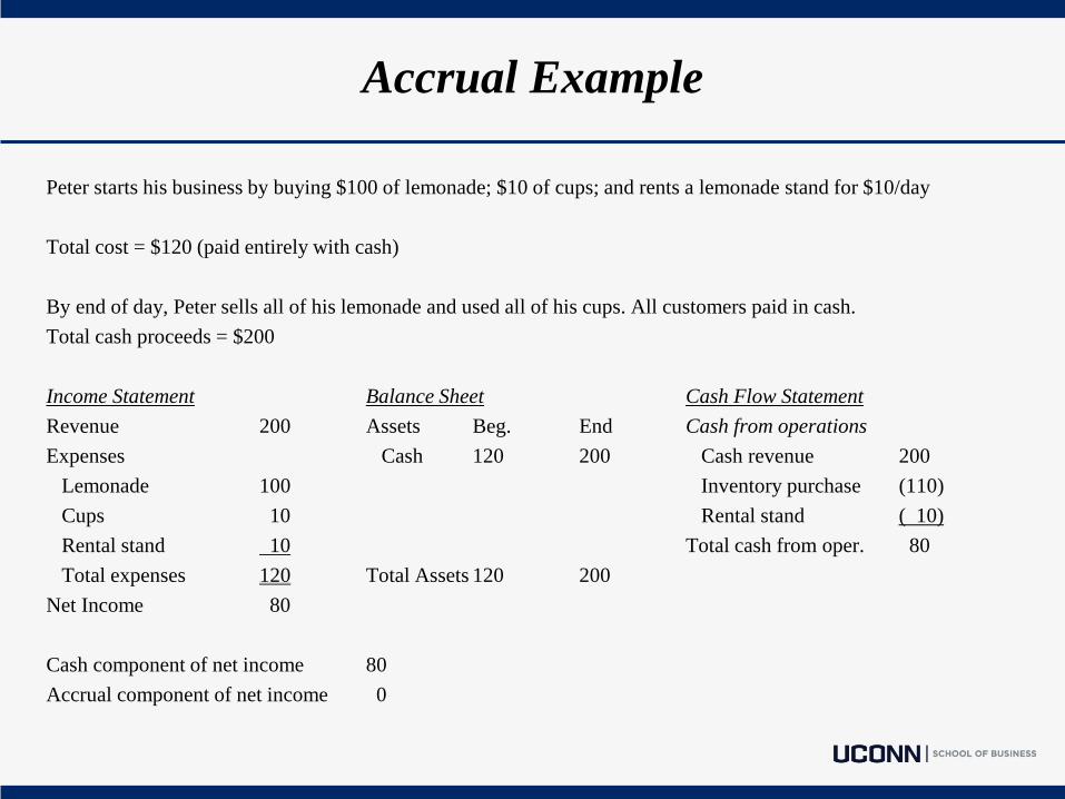
Peter starts his business by buying $100 of lemonade; $10 of cups; and rents a lemonade stand for $10/day
Total cost = $120 (paid entirely with cash)
By end of day, Peter sells all of his lemonade and used all of his cups. All customers paid in cash.
Total cash proceeds = $200
Income Statement Balance Sheet Cash Flow Statement
Revenue 200 Assets Beg. End Cash from operations
Expenses Cash 120 200 Cash revenue 200
Lemonade 100 Inventory purchase (110)
Cups 10 Rental stand ( 10)
Rental stand 10 Total cash from oper. 80
Total expenses 120 Total Assets 120 200
Net Income 80
Cash component of net income 80
Accrual component of net income 0

Accrual Example
Paul starts his business by buying $1,000 of lemonade; $100 of cups; and buys a lemonade stand for $1,000. He
expects the stand will be used for 100 days.
Total cost = $2,100 (paid entirely with cash)
By end of day, Peter sells 10% of his lemonade and used 10% of his cups. Peter generated $200 in revenue, but half
of his customers were short on cash and agreed to come back the next day to pay.
Income Statement Balance Sheet Cash Flow Statement
Revenue 200 Assets Beg. End Cash from operations
Expenses Cash 2,100 100 Cash revenue 100
Lemonade 100 A/R 100 Inventory purchase (1,100)
Cups 10 Inventory 990 Total cash from oper. (1,100)
Rental stand 10 PP&E 990 Cash from investing
Total expenses 120 Total Assets 2,100 2,180 Purchase of stand (1,000)
Net Income 80 Total change in cash (2,000)
Cash component of net income (2,000)
Accrual component of net income 2,080

Sloan (1996): Accrual Anomaly
Current Net Operating Assets = (Current Assets – Cash) – (Current Liabilities – Short-term debt – Income taxes/P)
Similar to our previous definition of non-cash working capital
Accruals = Current Net Operating Assets (End of this year) – Current Net Operating Assets (End of previous year)
Earnings = Accruals + Cash Flows
Basic proposition:
The accrual component of earnings is of lower quality than the cash flow component of earnings

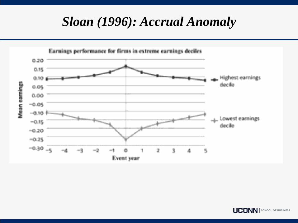
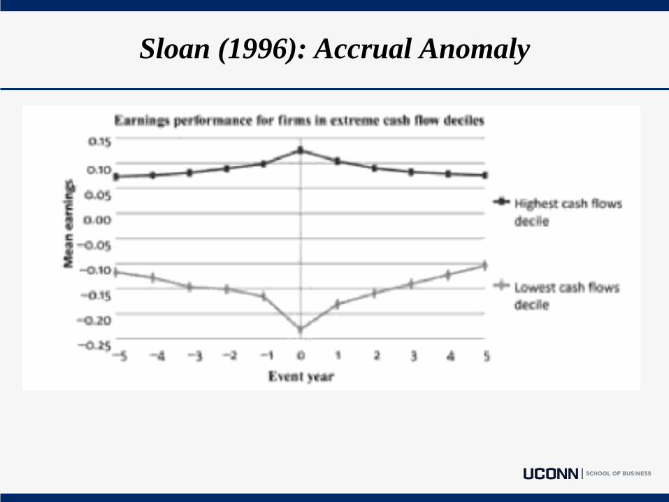
Sloan (1996): Accrual Anomaly
Large sample evidence
Event-time analysis
1. Compute earnings, accruals, and cash flows for a sample of firm-years from COMPUSTAT
2. Within each fiscal year, rank observations from lowest to highest based on earnings
3. Assign firm-years into deciles based on the rank of earnings,
decile 1: lowest-ranked 10%; decile 10: highest-ranked 10%
4. Compute the average level of earnings for firm-years in each decile
5. Track the average level of earnings for the corresponding set of firm-years in the surrounding 10 years (5 years
on either side of the ranking year)
6. Construct a plot of average earnings over the 11 years for the highest and lowest deciles
Sloan (1996): Accrual Anomaly

Sloan (1996): Accrual Anomaly
Sloan (1996): Accrual Anomaly
Sloan (1996): Accrual Anomaly
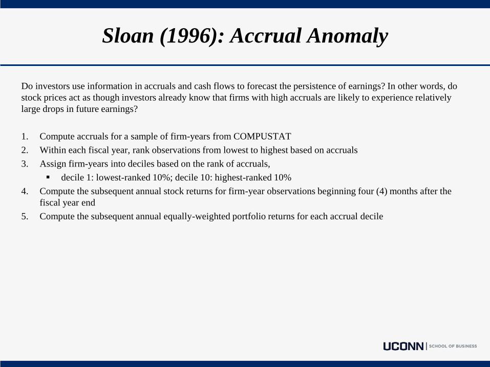
Do investors use information in accruals and cash flows to forecast the persistence of earnings? In other words, do
stock prices act as though investors already know that firms with high accruals are likely to experience relatively
large drops in future earnings?
1. Compute accruals for a sample of firm-years from COMPUSTAT
2. Within each fiscal year, rank observations from lowest to highest based on accruals
3. Assign firm-years into deciles based on the rank of accruals,
decile 1: lowest-ranked 10%; decile 10: highest-ranked 10%
4. Compute the subsequent annual stock returns for firm-year observations beginning four (4) months after the
fiscal year end
5. Compute the subsequent annual equally-weighted portfolio returns for each accrual decile
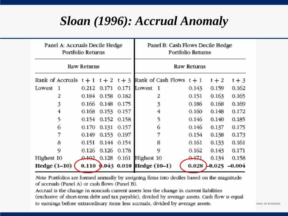
Sloan (1996): Accrual Anomaly

Sloan (1996): Accrual Anomaly
Note: Positive in 30 out of 38 years

Accrual Anomaly
Do sophisticated financial intermediaries (i.e., analysts, auditors, institutional investors) use
information in accruals?
Analysts
• Analysts are viewed as sophisticated interpreters of financial information
• Sell-side analysts appear to be largely oblivious to persistence of accruals
• Research has found that analyst earnings forecasts for firms with high accruals are far too optimistic
Auditors
• Auditors provide an opinion about whether firms’ earnings fairly present the results of their operations
• Research has found no evidence of a higher incidence of auditor qualifications or auditor changes in firms with
higher accruals
Institutional investors
• There is evidence that institutional investors do trade on the accrual anomaly, but the magnitude of trading (at
least 10 years ago) was relatively small
• Even though institutional investors dominate the corporate bond market, the accrual anomaly is also robust in
bond returns

Accrual Anomaly
Current net operating assets seems to be a limited definition of accruals. What happens when a
broader definition is applied?
• Using only current non-cash net operating assets: Hedge return is 13.3% per annum (sample specific)
• Using all non-cash net operating assets: Hedge return is 18% per annum (sample specific)
• Aggregating accruals over two years yields stronger results than using just one year
Where is the accrual anomaly the strongest?
• Research has found that inventory accruals exhibit the most robust relation with future stock returns
• ‘Discretionary’ accruals exhibit a stronger correlation with future returns than do ‘normal’ accruals

Accrual Anomaly
What future events drive the returns to the accrual anomaly?
• Extreme inventory accruals are more likely to experience extreme subsequent reversals
• High accrual firms are more likely to report negative special items over the next three (3) years
• High accrual firms are more likely to be targets of SEC enforcement actions
• When low accruals are driven by special items (i.e, write-offs and other unusual negative items), the low
accruals are less persistent – earnings will improve more quickly
Is the accrual anomaly robust in other countries?
• The accrual anomaly generates positive hedge returns in 85% of countries examined by prior research
• Appears stronger in common law (relative to code law) countries

Accrual Anomaly
Is the accrual anomaly still pervasive today? In other words, could I still make money on it?
• Yes and No
• The very simplistic approach taken by Sloan (1996) has been employed by a large number of hedge funds and
other institutional investors, so it has likely been arbitraged away.
• However, the basic premise of Sloan’s research still applies today.
• Fundamental analysis is likely to yield significant abnormal returns if applied in a robust, rigorous, novel
manner
• In Sloan’s day, investors appear to have been fixated on reported earnings (rather than earnings quality).
Today, although less naïve about the basic components of earnings, investors are still subject to behavioral
biases, information overload, limited attention, and other externalities that may prohibit high-quality
fundamental analysis.
Opportunities exist for successful trading strategies. You just have to be willing to put in the work and go find
them…

Hypothetical Situation
Assume you are the CEO of a Fortune 500 company.
Further assume that upon waking up on a Wednesday morning in November, you recognize that your firm’s stock
price is too high (overvalued)? What actions, if any, do you take given this piece of information?
Next, consider the same hypothetical situation as above, only this time your firm’s stock price is undervalued. What
actions, if any, do you take given this piece of information?

Net Stock Anomalies
Significant Corporate Events (financing policy decisions):
Initial Public Offerings (IPOs)
Seasoned Equity Offerings (SEOs)
Debt Issuances
Share Repurchases and Tender Offers
Dividend Initiation and Omissions
Private Equity Placement
Overall Net External Financing
Mergers and Acquisitions

Initial Public Offerings
IPOs tend to significantly underperform the market. Why?
Are investors too optimistic?
Were (pre-IPO) earnings managed upward?
• IPOs with lower quality earnings underperformed IPOs with higher quality earnings
What role to VCs (venture-capital) play in IPO firms’ subsequent performance?
• VC-backed IPOs outperform non-VC-backed IPOs
Market-Timing Hypothesis
• Periods of high equity share (of total volume of debt and equity issuances) are followed by low
returns. Managers may be able to time equity offerings during market peaks.
Note: IPOS tend to cluster during periods when firms seem to be able to raise money at favorable
prices. Even though this clustering may contribute to an ex post market peak, managers do not
necessarily have to forecast market movements ex ante.
Seasoned Equity Offerings
Firms issuing equity through an SEO experience negative future stock returns. Why?
Are opportunistic managers exploiting their firms’ overvaluation?
• In the year prior to the SEO, stock returns average +72% (according to Loughran and Ritter 1995)
Is overvaluation in this setting driven by earnings management?
SEOs affect overall firm risk
• Decreased leverage (following an equity issuance) reduces the firm’s systematic risk

Debt Issuances
Firms issuing debt (public or private) experience negative future stock returns. Why?
Effect is exacerbated among younger and smaller firms
Similar to equity issuances, debt equity offerings (convertible debt) may be a signal of overvaluation
Firms calling straight or convertible debt outperform their peers

Share Repurchases and Tender Offers
Open market share repurchases and self-tender offer announcements yield significant abnormal stock returns. Why?
Contrary to equity issuances, share repurchases may be a signal of undervaluation
• Alternatively, repurchases may be used to manager reported eps or avoid paying dividends
Repurchasing firms earn significant positive abnormal returns after the repurchase
• Effect is concentrated among small firms
Large firms experience positive abnormal returns before the repurchase (zero abnormal returns afterward)
Open market repurchases yield positive future returns
• Firms more likely to repurchase due to undervaluation earn significantly higher future returns

Dividend Initiation and Omissions
Similar to reporting a positive (negative) earnings surprise, firms with dividend initiations (omissions) experience
positive (negative) future returns. Why?
Stock price reaction is asymmetric
• Reaction is more extreme for omissions, relative to initiations
• Price continues to drift in same direction for up to three years
Past performance drives the dividend decision
• Dividend initiators significantly outperform the market in prior year
• Dividend omitters significantly underperform the market in prior year
Private Equity Placement
Following positive announcement period returns, firms that engage in private placement of equity experience
significant negative future returns. Why?
Underperformance is similar to the IPO and SEO setting
Investors may be overoptimistic about firms’ growth prospects
• Private placement firms tend to invest more than control groups
Unlike public offerings, private issues tend to follow periods of relatively poor operating performance

Overall Net External Financing
Net External Financing is a strong predictor of future stock returns. Why?
Net External Financing = Net cash received from sale or purchase of common and preferred stock – cash
dividends paid + net cash received from the issuance of or retirement of debt
Hedge portfolio going long in lowest decile (net repurchasers) and short in highest decile (net issuers)
yield significant abnormal returns
Net external financing is positively correlated with analyst optimism
• Overoptimism for debt issuances is restricted to short-term forecasts
• Overoptimism for equity issuances is also related to long-term earnings forecasts, growth, stock
recommendations, and target prices
Misvaluation Hypothesis
• Firms may time corporate financing activities to exploit temporary misvaluations of firms’
securities in capital markets
Note: Some research suggests that since financing and operating cash flows are negatively correlated, the net
external financing anomaly is simply a variation of the widely-accepted accrual anomaly (and consistent with
the overinvestment hypothesis).

Mergers and Acquisitions
Acquiring firms experience significant negative future returns. Why?
Acquiring firms experience unusually high stock price performance leading up to bid announcement.
• Poses research design issues when prior stock price movement and event are not independent of
each other
Cash tender offer yield positive future returns, whereas stock mergers generate significantly negative
abnormal returns
Performance Extrapolation Hypothesis
• Capital market over-extrapolates bidders’ past performance when valuing the deal
‘Interesting’ Research Findings
Carroll et al. (2002) show that admissions for heart attacks increased 25% during the 3-day period starting June
30, 1998, the day England lost to Argentina in a World Cup penalty shoot-out
Hirt et al. (1992) find that Indiana University college students estimate their own performance to be
significantly better after watching a win by their college basketball team than after watching a loss
Schweitzer et al. (1992) shows that assessments of both the probability of a 1990 war in Iraq and its potential
casualties were significantly lower among students rooting for the winning team of a televised American
football game than among fans of the losing team
Benos and Jochev (2013) find that companies whose names contain the words “America(n)” or “USA” earn
positive abnormal returns of about 6% per annum during World War II, the Korean War, and the War on
Terrorism
Arkes, Herren, and Isen (1988) find that sales of Ohio State lottery tickets increase in the days after a victory
by the Ohio State University football team
White (1989) documents that elimination from the U.S. National Football League playoffs leads to a significant
increase in homicides in the relevant cities following the games
Trovato (1998) also finds that suicides among Canadians rise significantly if the Montreal Canadians are
eliminated early from the Stanley Cup playoffs

‘Interesting’ Research Findings
Maymin (2012) compares the annual average beat variance of the songs in the U.S. Billboard Top 100 since its
inception in 1958 through 2007 to the standard deviation of returns of the S&P 500 for the same or the
subsequent year, and finds a significant negative correlation.
Excerpt from Abstract: In a field quasi-experiment 18–25-year-old women walking alone in the street were
approached by an attractive 20-year-old male confederate who solicited them for their phone numbers. The
women were solicited on days that were evaluated as being either sunny or cloudy but care was taken to control
for temperature and not to solicit participants when it rained. It was found that women agreed more often to the
confederate's courtship solicitation on the sunny days. Positive mood induction by the sun may explain such
results. - Nicolas Guéguen (2013)
Excerpt from Abstract: Superstitious beliefs persist if they are not exposed as untrue. This paper investigates
whether Chinese superstition that the number 4 is unlucky and number 8 is lucky affects the Singapore housing
market. We find that Singaporean Chinese are less likely to buy units and on floors with numbers ending in 4.
The prices of residential units with numbers ending in 4 exhibit a discount of 1.1% while those with numbers
ending in 8 exhibit a premium of 0.9%. Residents of lucky-numbered homes are no less likely to experience car
accidents as residents of unlucky-numbered homes, which suggest that equilibrium choices and prices are in
fact based on irrational beliefs. - Agarwal et.al (2014 WP)

Seasonal Anomalies
Significant Seasonal Anomalies detected in recent past:
January Effect
January Barometer
Sell in May and Go Away
Holiday effects
Day of week effects
Political effects
Turn of the month effects
Weather effects

January Effect
Small cap stocks outperform large caps in the month of January. Why?
Tax effects
Portfolio rebalancing
Disclosure
Bonus compensation

January Barometer
If stock market rises in January, it will continue the rise for the rest of the year.
71 Years (1940-2010)
44 years January up
38 years (86.4%) Rest of Year UP
6 years (13.6%) Rest of Year DOWN
27 years January down
14 years (51.9%) Rest of Year UP
13 years (48.1%) Rest of Year DOWN
Sell in May and Go Away
September and October historically have low stock returns
November- February historically have higher stock returns

Holiday Effects
Significant positive abnormal returns on pre-holiday days
Underperformance during Rosh Hashanah
Outperformance during Ramadan
Research: Frieder and Subrahmanyam (2004) find abnormally positive returns around Yom Kippur and St.
Patrick's Day and negative returns around Rosh Hashanah

Day of the Week Effects
Monday: Low returns (mostly during final two Mondays of the month)
Friday: High returns
Possibly driven by short sellers?
Tuesday – Friday: Stocks advance during first 45 minutes of trading
Monday: Stocks fall during first 45 minutes of trading
All days: Stocks advance near the end of the day
Political Effects
Returns are lower and volatility is higher when Congress is in session
Public opinion of Congress matters
Positive short-term returns following Republican victories
Negative short-term returns following Democrat victories
Higher stock returns during last two years of political campaign than during first two years
Small cap stocks perform better during Democratic administrations

Turn of the Month Effect
In general, stock have higher returns around the turn of the month (-1 - +3)
U.S. economy pays out money on t-1
Portfolio window dressing

Weather Effects
Sunshine is positively correlated with daily returns
Stock returns are lower on days around a full moon compared to days around a new moon

Sports Effects
Loss in World Cup (soccer) elimination games leads to next day abnormal returns of -49 bps
Similar negative effect for international cricket, rugby, and basketball games
Firms sponsoring successful NASCAR racing teams earn positive abnormal returns
National Football League (NFL) team’s losses leads to lower next-day returns for locally headquartered stocks
Recommended