ACCT 420: Logistic
Regression for Corporate
Fraud
Session 6
Dr. Richard M. Crowley
1

Front matter
2 . 1

▪ Theory:
▪ Economics
▪ Psychology
▪ Application:
▪ Predicting fraud contained
in annual reports
▪ Methodology:
▪ Logistic regression
▪ LASSO
Learning objectives
2 . 2

Datacamp
▪ Explore on your own
▪ No specific required class this week
2 . 3

Corporate/Securities Fraud
3 . 1
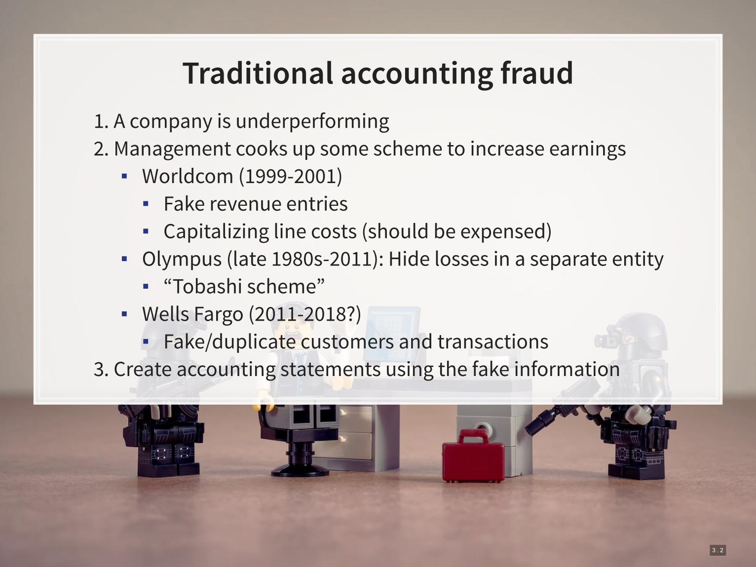
Traditional accounting fraud
1. A company is underperforming
2. Management cooks up some scheme to increase earnings
▪ Worldcom (1999-2001)
▪ Fake revenue entries
▪ Capitalizing line costs (should be expensed)
▪ Olympus (late 1980s-2011): Hide losses in a separate entity
▪ “Tobashi scheme”
▪ Wells Fargo (2011-2018?)
▪ Fake/duplicate customers and transactions
3. Create accounting statements using the fake information
3 . 2

Reversing it
1. A company is overperforming
2. Management cooks up a scheme to “save up” excess performance for
a rainy day
▪
▪ Cookie jar reserve, from secret payments by Intel, made up to
76% of quarterly income
▪
3. Recognize revenue/earnings when needed in the future to hit earnings
targets
Dell (2002-2007)
Brystol-Myers Squibb (2000-2001)
3 . 3

Other accounting fraud types
▪
▪ Options backdating
▪
▪ Using an auditor that isn’t registered
▪
▪ Releasing financial statements that were not reviewed by an auditor
▪
▪ Related party transactions (transferring funds to family members)
▪ Insufficient internal controls
▪ via Banamex
▪
Apple (2001)
Commerce Group Corp (2003)
Cardiff International (2017)
China North East Petroleum Holdings Limited
Citigroup (2008-2014)
Asia Pacific Breweries
3 . 4

Other accounting fraud types
▪
▪ Round-tripping: Transactions to inflate revenue that have no
substance
▪ Bribery
▪ : $55M USD in bribes to Brazilian officials
for contracts
▪ Baker Hughes ( , ): Payments to officials in Indonesia, and
possibly to Brazil and India (2001) and to officials in Angola,
Indonesia, Nigeria, Russia, and Uzbekistan (2007)
▪ : Fake the whole company, get funding from
insurance fraud, the�, credit card fraud, and fake contracts
▪ Also faked a real project to get a clean audit to take the company
public
Suprema Specialties (1998-2001)
Keppel O&M (2001-2014)
2001 2007
ZZZZ Best (1982-1987)
3 . 5

Other securities fraud types
▪ : Ponzi scheme
1. Get money from individuals for “investments”
2. Pretend as though the money was invested
3. Use new investors’ money to pay back anyone withdrawing their
money
▪
▪ Material misstatements
▪ Material omissions (FDA applications, didn’t pay payroll taxes)
▪
▪ Failed to file annual and quarterly reports
▪
▪ Aiding another company’s fraud (Take Two, by parking 2 video
games)
▪
▪ Misleading statements on Twitter
Bernard Madoff
Imaging Diagnostic Systems (2013)
Applied Wellness Corporation (2008)
Capitol Distributing LLC
Tesla (2018)
3 . 6

Some of the more interesting cases
▪
▪ Claimed it was developing processor microcode independently,
when it actually provided Intel’s microcode to it’s engineers
▪
▪ Sham sale-leaseback of a bar to a corporate officer
▪
▪ Not using mark-to-market accounting to fair value stuffed animal
inventories
▪
▪ Gold reserves were actually… dirt.
▪
▪ Employees created 1,280 fake memberships, sold them, and
retained all profits ($37.5M)
AMD (1992-1993)
Am-Pac International (1997)
CVS (2000)
Countryland Wellness Resorts, Inc. (1997-2000)
Keppel Club (2014)
3 . 7

What will we look at today?
Misstatements: Errors that affect firms’ accounting
statements or disclosures which were done seemingly
intentionally by management or other employees at the
firm.
3 . 8

How do misstatements come to light?
1. The company/management admits to it publicly
2. A government entity forces the company to disclose
▪ In more egregious cases, government agencies may disclose the
fraud publicly as well
3. Investors sue the firm, forcing disclosure
3 . 9
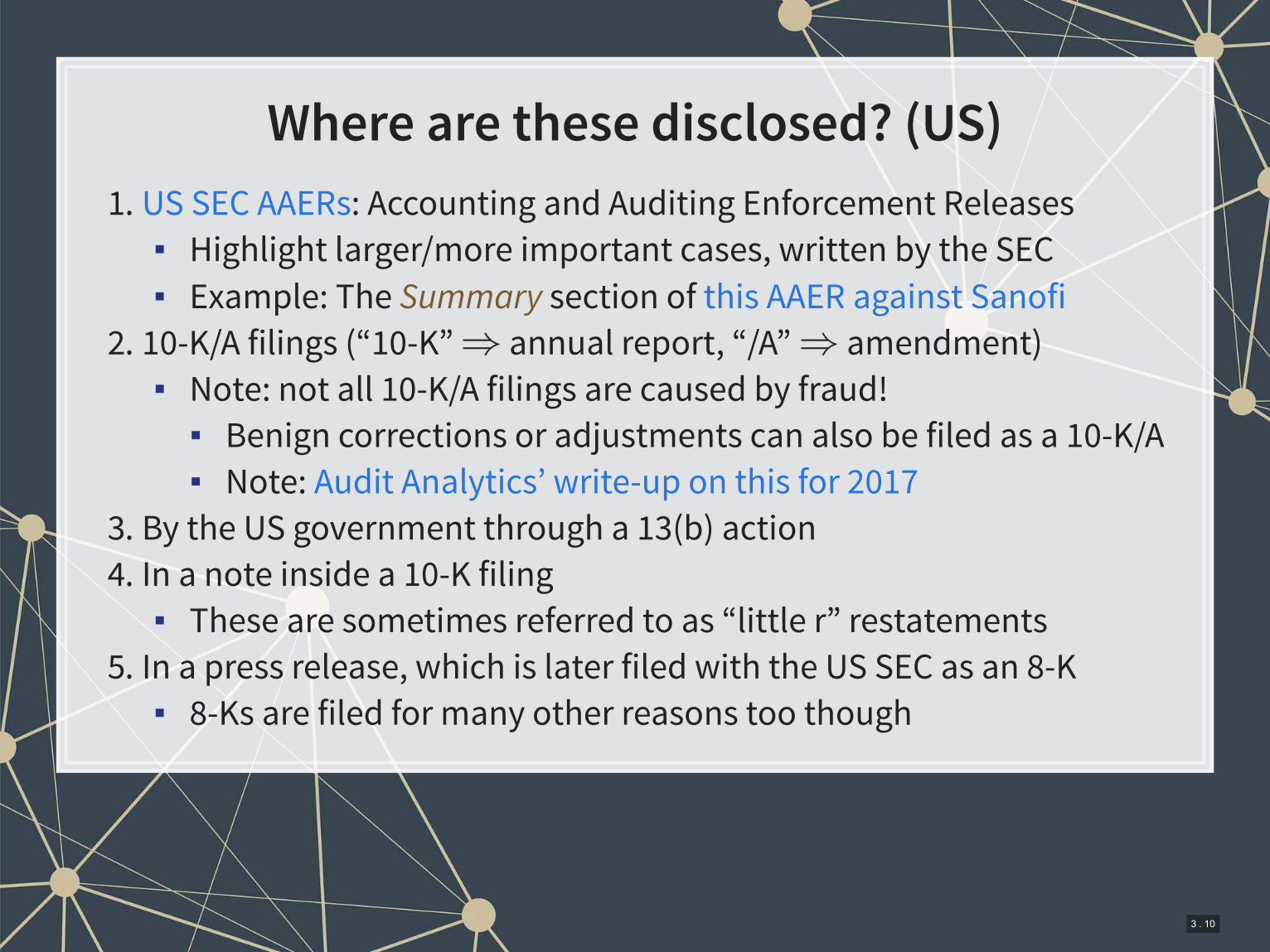
Where are these disclosed? (US)
1. : Accounting and Auditing Enforcement Releases
▪ Highlight larger/more important cases, written by the SEC
▪ Example: The Summary section of
2. 10-K/A filings (“10-K” annual report, “/A” amendment)
▪ Note: not all 10-K/A filings are caused by fraud!
▪ Benign corrections or adjustments can also be filed as a 10-K/A
▪ Note:
3. By the US government through a 13(b) action
4. In a note inside a 10-K filing
▪ These are sometimes referred to as “little r” restatements
5. In a press release, which is later filed with the US SEC as an 8-K
▪ 8-Ks are filed for many other reasons too though
US SEC AAERs
this AAER against Sanofi
Audit Analytics’ write-up on this for 2017
3 . 10

Where are we at?
▪ All of them are important to capture
▪ All of them affect accounting numbers differently
▪ None of the individual methods are frequent…
▪ We need to be careful here (or check multiple sources)
Fraud happens in many ways, for many reasons
It is disclosed in many places. All have subtly different
meanings and implications
This is a hard problem!
3 . 11

AAERs
▪ Today we will examine these AAERs
▪ Using a proprietary data set of >1,000 such releases
▪ To get a sense of the data we’re working with, read the Summary
section (starting on page 2) of this AAER against Sanofi
▪ rmc.link/420class7
Why did the SEC release this AAER regarding Sanofi?
3 . 12

Predicting Fraud
4 . 1

Main question
▪ This is a pure forensic analytics question
▪ “Major instance of misreporting” will be implemented using AAERs
How can we detect if a firm is involved in a major instance
of missreporting?
4 . 2

Approaches
▪ In these slides, I’ll walk through the primary detection methods since
the 1990s, up to currently used methods
▪ 1990s: Financials and financial ratios
▪ Follow up in 2011
▪ Late 2000s/early 2010s: Characteristics of firm’s disclosures
▪ mid 2010s: More holistic text-based measures of disclosures
▪ This will tie to next lesson where we will explore how to work with
text
All of these are discussed in a
– I will refer to the paper as BCE for short
Brown, Crowley and Elliott
(2019)
4 . 3

The data
▪ I have provided some preprocessed data, sanitized of AAER data
(which is partially public, partially proprietary)
▪ It contains 401 variables
▪ From Compustat, CRSP, and the SEC (which I personally collected)
▪ Many precalculated measures including:
▪ Firm characteristics, such as auditor type (bigNaudit,
midNaudit)
▪ Financial measures, such as total accruals (rsst_acc)
▪ Financial ratios, such as ROA (ni_at)
▪ Annual report characteristics, such as the mean sentence length
(sentlen_u)
▪ Machine learning based content analysis (everything with
Topic_ prepended)
Pulled from BCE’s working files
4 . 4

Training and Testing
▪ Already has testing and training set up in variable Test
▪ Training is annual reports released in 1999 through 2003
▪ Testing is annual reports released in 2004
What potential issues are there with our usual training and
testing strategy?
4 . 5

Censoring
▪ Censoring training data helps to emulate historical situations
▪ Build an algorithm using only the data that was available at the
time a decision would need to have been made
▪ Do not censor the testing data
▪ Testing emulates where we want to make an optimal choice in real
life
▪ We want to find frauds regardless of how well hidden they are!
4 . 6
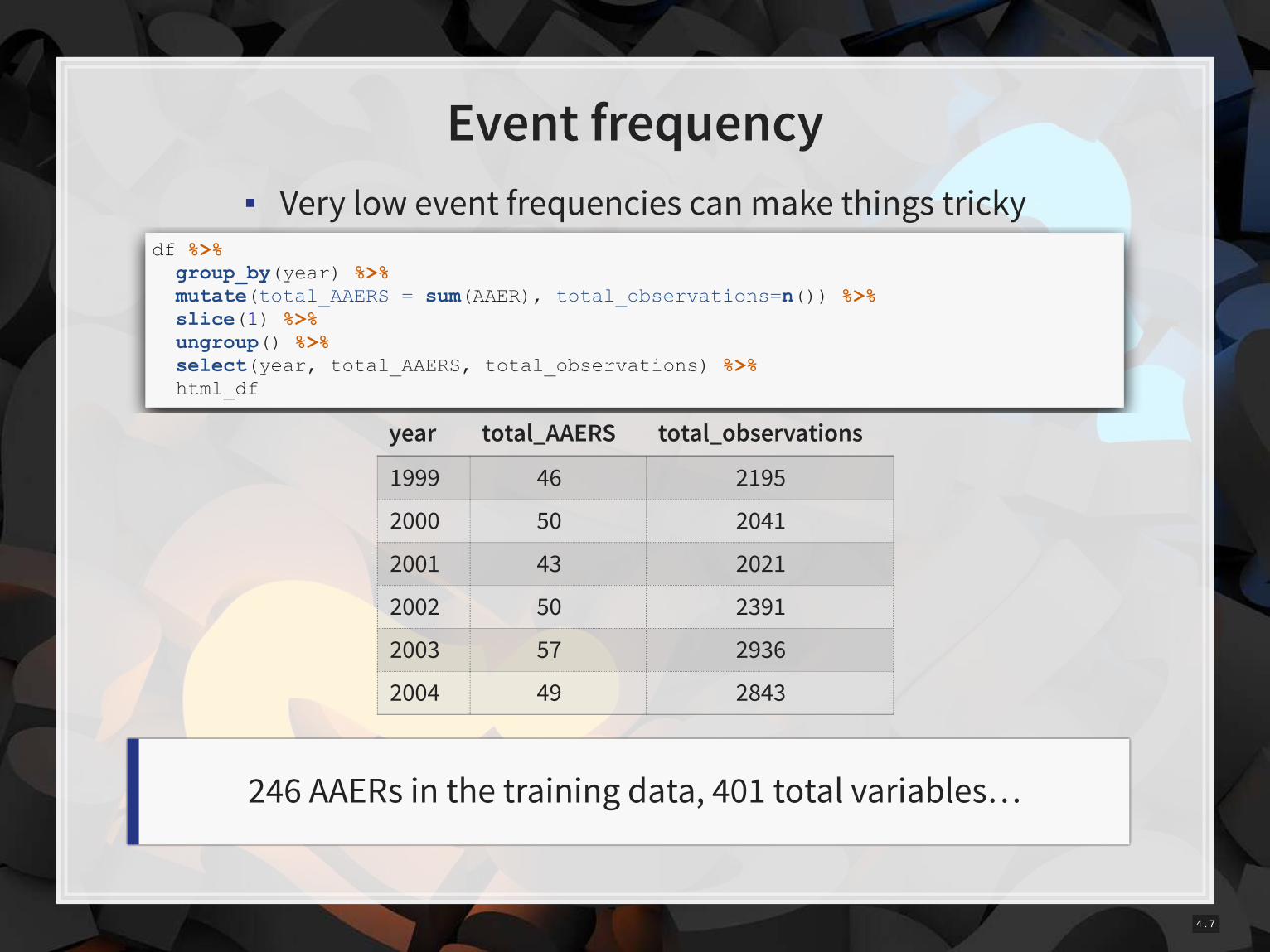
Event frequency
▪ Very low event frequencies can make things tricky
year total_AAERS total_observations
1999 46 2195
2000 50 2041
2001 43 2021
2002 50 2391
2003 57 2936
2004 49 2843
df %>% group_by(year) %>% mutate(total_AAERS = sum(AAER), total_observations=n()) %>% slice(1) %>% ungroup() %>% select(year, total_AAERS, total_observations) %>% html_df
246 AAERs in the training data, 401 total variables…
4 . 7

Dealing with infrequent events
▪ A few ways to handle this
1. Very careful model selection (keep it sufficiently simple)
2. Sophisticated degenerate variable identification criterion +
simulation to implement complex models that are just barely
simple enough
▪ The main method in BCE
3. Automated methodologies for pairing down models
▪ We’ll discuss using LASSO for this at the end of class
▪ Also implemented in BCE
4 . 8

1990s approach
5 . 1
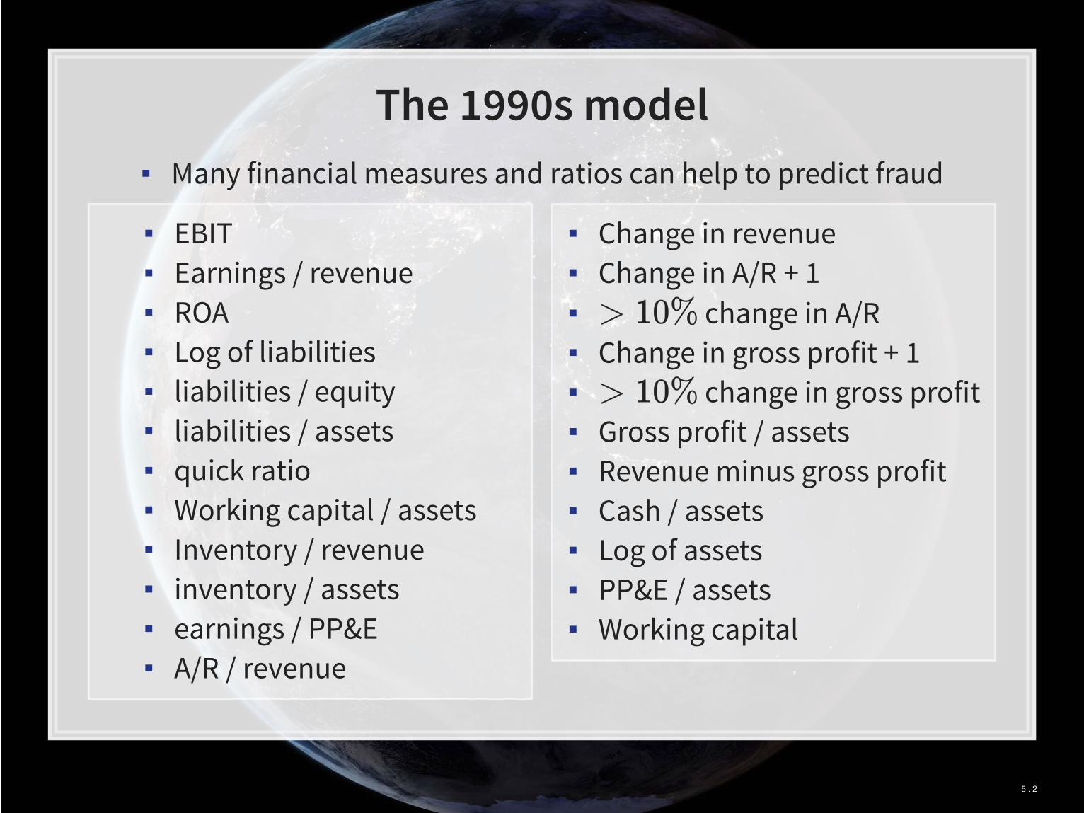
▪ EBIT
▪ Earnings / revenue
▪ ROA
▪ Log of liabilities
▪ liabilities / equity
▪ liabilities / assets
▪ quick ratio
▪ Working capital / assets
▪ Inventory / revenue
▪ inventory / assets
▪ earnings / PP&E
▪ A/R / revenue
▪ Change in revenue
▪ Change in A/R + 1
▪ change in A/R
▪ Change in gross profit + 1
▪ change in gross profit
▪ Gross profit / assets
▪ Revenue minus gross profit
▪ Cash / assets
▪ Log of assets
▪ PP&E / assets
▪ Working capital
The 1990s model
▪ Many financial measures and ratios can help to predict fraud
5 . 2

Approach
fit_1990s <- glm(AAER ~ ebit + ni_revt + ni_at + log_lt + ltl_at + lt_seq + lt_at + act_lct + aq_lct + wcap_at + invt_revt + invt_at + ni_ppent + rect_revt + revt_at + d_revt + b_rect + b_rect + r_gp + b_gp + gp_at + revt_m_gp + ch_at + log_at + ppent_at + wcap, data=df[df$Test==0,], family=binomial) summary(fit_1990s)
## ## Call: ## glm(formula = AAER ~ ebit + ni_revt + ni_at + log_lt + ltl_at + ## lt_seq + lt_at + act_lct + aq_lct + wcap_at + invt_revt + ## invt_at + ni_ppent + rect_revt + revt_at + d_revt + b_rect + ## b_rect + r_gp + b_gp + gp_at + revt_m_gp + ch_at + log_at + ## ppent_at + wcap, family = binomial, data = df[df$Test == ## 0, ]) ## ## Deviance Residuals: ## Min 1Q Median 3Q Max ## -1.1391 -0.2275 -0.1661 -0.1190 3.6236 ## ## Coefficients: ## Estimate Std. Error z value Pr(>|z|) ## (Intercept) -4.660e+00 8.336e-01 -5.591 2.26e-08 *** ## ebit -3.564e-04 1.094e-04 -3.257 0.00112 ** ## ni_revt 3.664e-02 3.058e-02 1.198 0.23084 ## ni_at -3.196e-01 2.325e-01 -1.374 0.16932 ## log_lt 1.494e-01 3.409e-01 0.438 0.66118 ## ltl at -2.306e-01 7.072e-01 -0.326 0.74438
5 . 3

ROC
## In sample AUC Out of sample AUC ## 0.7483132 0.7292981
5 . 4

The 2011 follow up
6 . 1

▪ Log of assets
▪ Total accruals
▪ % change in A/R
▪ % change in inventory
▪ % so� assets
▪ % change in sales from cash
▪ % change in ROA
▪ Indicator for stock/bond
issuance
▪ Indicator for operating leases
▪ BV equity / MV equity
▪ Lag of stock return minus
value weighted market return
▪ Below are BCE’s additions
▪ Indicator for mergers
▪ Indicator for Big N auditor
▪ Indicator for medium size
auditor
▪ Total financing raised
▪ Net amount of new capital
raised
▪ Indicator for restructuring
The 2011 model
Based on Dechow, Ge, Larson and Sloan (2011)
6 . 2

The model
fit_2011 <- glm(AAER ~ logtotasset + rsst_acc + chg_recv + chg_inv + soft_assets + pct_chg_cashsales + chg_roa + issuance + oplease_dum + book_mkt + lag_sdvol + merger + bigNaudit + midNaudit + cffin + exfin + restruct, data=df[df$Test==0,], family=binomial) summary(fit_2011)
## ## Call: ## glm(formula = AAER ~ logtotasset + rsst_acc + chg_recv + chg_inv + ## soft_assets + pct_chg_cashsales + chg_roa + issuance + oplease_dum + ## book_mkt + lag_sdvol + merger + bigNaudit + midNaudit + cffin + ## exfin + restruct, family = binomial, data = df[df$Test == ## 0, ]) ## ## Deviance Residuals: ## Min 1Q Median 3Q Max ## -0.8434 -0.2291 -0.1658 -0.1196 3.2614 ## ## Coefficients: ## Estimate Std. Error z value Pr(>|z|) ## (Intercept) -7.1474558 0.5337491 -13.391 < 2e-16 *** ## logtotasset 0.3214322 0.0355467 9.043 < 2e-16 *** ## rsst_acc -0.2190095 0.3009287 -0.728 0.4667 ## chg_recv 1.1020740 1.0590837 1.041 0.2981 ## chg_inv 0.0389504 1.2507142 0.031 0.9752 ## soft_assets 2.3094551 0.3325731 6.944 3.81e-12 *** ## pct chg cashsales -0.0006912 0.0108771 -0.064 0.9493
6 . 3
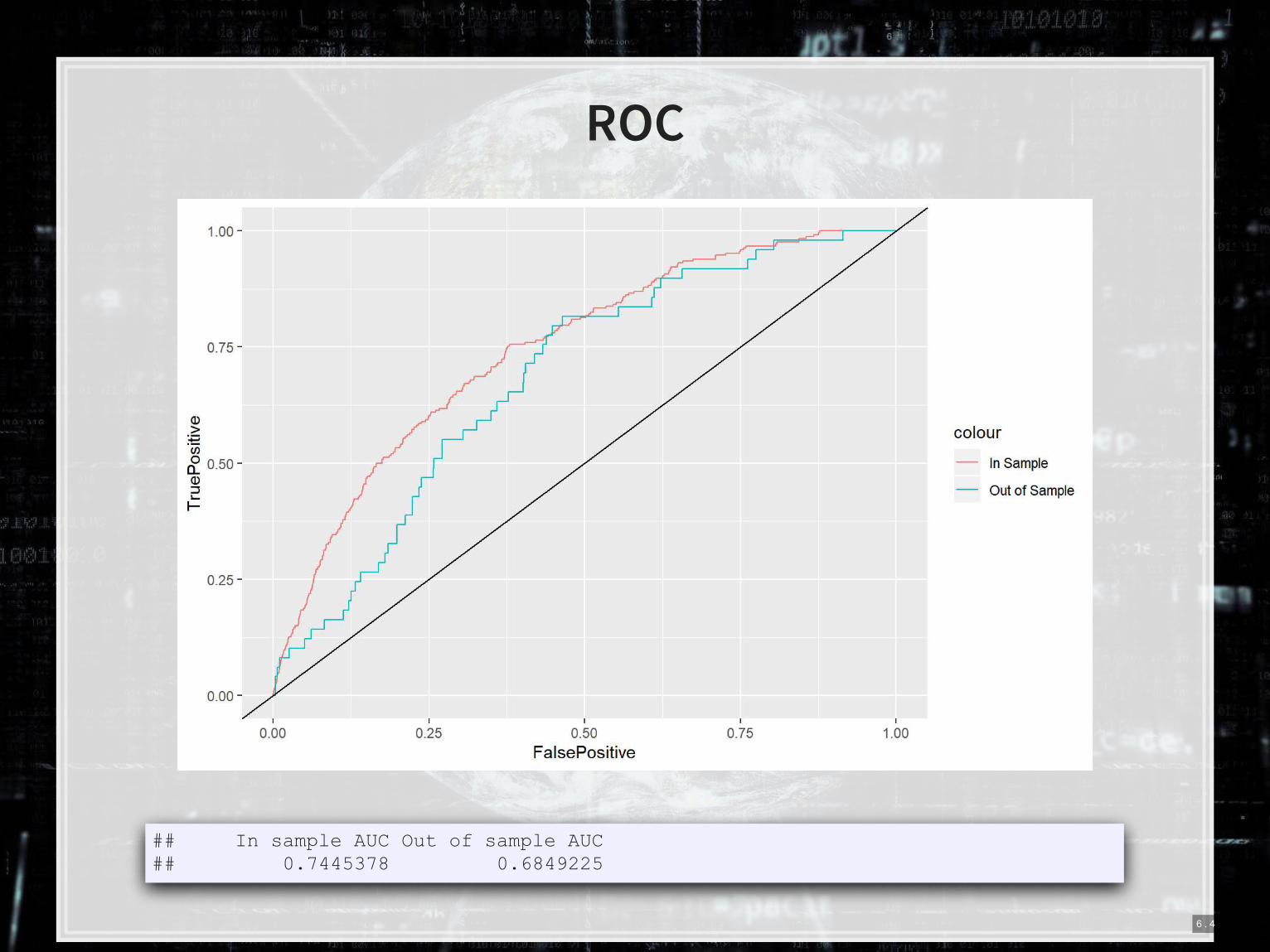
ROC
## In sample AUC Out of sample AUC ## 0.7445378 0.6849225
6 . 4

Late 2000s/early 2010s approach
7 . 1

▪ Log of # of bullet points + 1
▪ # of characters in file header
▪ # of excess newlines
▪ Amount of html tags
▪ Length of cleaned file,
characters
▪ Mean sentence length, words
▪ S.D. of word length
▪ S.D. of paragraph length
(sentences)
▪ Word choice variation
▪ Readability
▪ Coleman Liau Index
▪ Fog Index
▪ % active voice sentences
▪ % passive voice sentences
▪ # of all cap words
▪ # of !
▪ # of ?
The late 2000s/early 2010s model
From a variety of papers
7 . 2
Theory
▪ Generally pulled from the communications literature
▪ Sometimes ad hoc
▪ The main idea:
▪ Companies that are misreporting probably write their annual report
differently
7 . 3
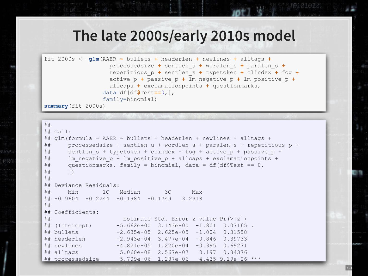
The late 2000s/early 2010s model
fit_2000s <- glm(AAER ~ bullets + headerlen + newlines + alltags + processedsize + sentlen_u + wordlen_s + paralen_s + repetitious_p + sentlen_s + typetoken + clindex + fog + active_p + passive_p + lm_negative_p + lm_positive_p + allcaps + exclamationpoints + questionmarks, data=df[df$Test==0,], family=binomial) summary(fit_2000s)
## ## Call: ## glm(formula = AAER ~ bullets + headerlen + newlines + alltags + ## processedsize + sentlen_u + wordlen_s + paralen_s + repetitious_p + ## sentlen_s + typetoken + clindex + fog + active_p + passive_p + ## lm_negative_p + lm_positive_p + allcaps + exclamationpoints + ## questionmarks, family = binomial, data = df[df$Test == 0, ## ]) ## ## Deviance Residuals: ## Min 1Q Median 3Q Max ## -0.9604 -0.2244 -0.1984 -0.1749 3.2318 ## ## Coefficients: ## Estimate Std. Error z value Pr(>|z|) ## (Intercept) -5.662e+00 3.143e+00 -1.801 0.07165 . ## bullets -2.635e-05 2.625e-05 -1.004 0.31558 ## headerlen -2.943e-04 3.477e-04 -0.846 0.39733 ## newlines -4.821e-05 1.220e-04 -0.395 0.69271 ## alltags 5.060e-08 2.567e-07 0.197 0.84376 ## processedsize 5.709e-06 1.287e-06 4.435 9.19e-06 ***
7 . 4
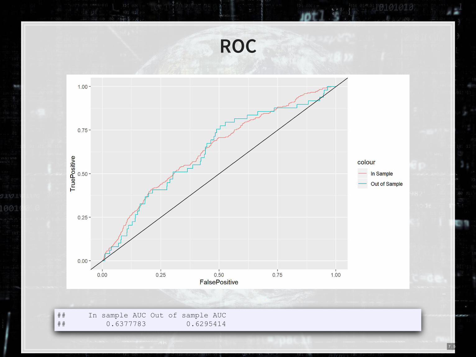
ROC
## In sample AUC Out of sample AUC ## 0.6377783 0.6295414
7 . 5

Combining the 2000s and 2011 models
▪ 2011 model: Parsimonious financial model
▪ 2000s model: Textual characteristics
Why is it appropriate to combine the 2011 model with the
2000s model?
7 . 6

The model
fit_2000f <- glm(AAER ~ logtotasset + rsst_acc + chg_recv + chg_inv + soft_assets + pct_chg_cashsales + chg_roa + issuance + oplease_dum + book_mkt + lag_sdvol + merger + bigNaudit + midNaudit + cffin + exfin + restruct + bullets + headerlen + newlines + alltags + processedsize + sentlen_u + wordlen_s + paralen_s + repetitious_p + sentlen_s + typetoken + clindex + fog + active_p + passive_p + lm_negative_p + lm_positive_p + allcaps + exclamationpoints + questionmarks, data=df[df$Test==0,], family=binomial) summary(fit_2000f)
## ## Call: ## glm(formula = AAER ~ logtotasset + rsst_acc + chg_recv + chg_inv + ## soft_assets + pct_chg_cashsales + chg_roa + issuance + oplease_dum + ## book_mkt + lag_sdvol + merger + bigNaudit + midNaudit + cffin + ## exfin + restruct + bullets + headerlen + newlines + alltags + ## processedsize + sentlen_u + wordlen_s + paralen_s + repetitious_p + ## sentlen_s + typetoken + clindex + fog + active_p + passive_p + ## lm_negative_p + lm_positive_p + allcaps + exclamationpoints + ## questionmarks, family = binomial, data = df[df$Test == 0, ## ]) ## ## Deviance Residuals: ## Min 1Q Median 3Q Max ## -0.9514 -0.2237 -0.1596 -0.1110 3.3882 ## ## Coefficients: ## Estimate Std. Error z value Pr(>|z|) ## (Intercept) -1.634e+00 3.415e+00 -0.479 0.63223 ## logtotasset 3.437e-01 3.921e-02 8.766 < 2e-16 ***
7 . 7

ROC
## In sample AUC Out of sample AUC ## 0.7664115 0.7147021
7 . 8

The BCE model
8 . 1
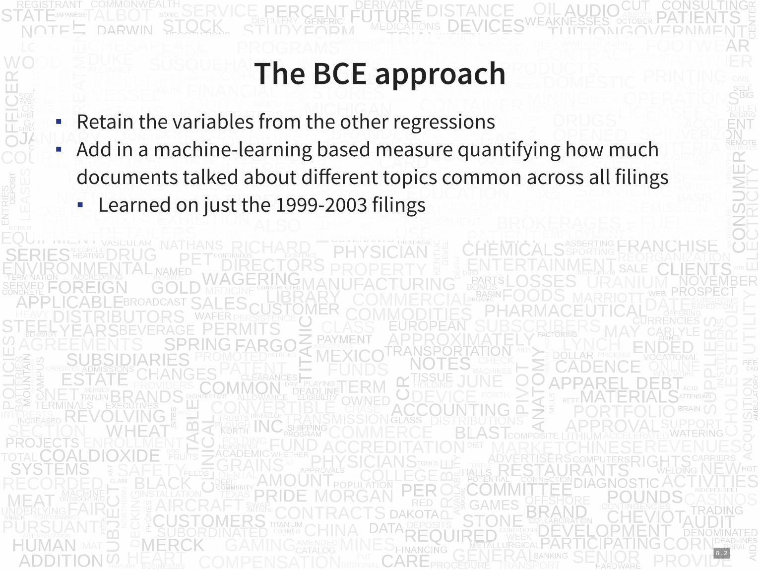
The BCE approach
▪ Retain the variables from the other regressions
▪ Add in a machine-learning based measure quantifying how much
documents talked about different topics common across all filings
▪ Learned on just the 1999-2003 filings
8 . 2

What the topics look like
8 . 3

Theory behind the BCE model
Why use document content?
8 . 4

The model
BCE_eq = as.formula(paste("AAER ~ logtotasset + rsst_acc + chg_recv + chg_inv + soft_assets + pct_chg_cashsales + chg_roa + issuance + oplease_dum + book_mkt + lag_sdvol + merger + bigNaudit + midNaudit + cffin + exfin + restruct + bullets + headerlen + newlines + alltags + processedsize + sentlen_u + wordlen_s + paralen_s + repetitious_p + sentlen_s + typetoken + clindex + fog + active_p + passive_p + lm_negative_p + lm_positive_p + allcaps + exclamationpoints + questionmarks + ", paste(paste0("Topic_",1:30,"_n_oI"), collapse=" + "), collapse="")) fit_BCE <- glm(BCE_eq, data=df[df$Test==0,], family=binomial) summary(fit_BCE)
## ## Call: ## glm(formula = BCE_eq, family = binomial, data = df[df$Test == ## 0, ]) ## ## Deviance Residuals: ## Min 1Q Median 3Q Max ## -1.0887 -0.2212 -0.1478 -0.0940 3.5401 ## ## Coefficients: ## Estimate Std. Error z value Pr(>|z|) ## (Intercept) -8.032e+00 3.872e+00 -2.074 0.03806 * ## logtotasset 3.879e-01 4.554e-02 8.519 < 2e-16 *** ## rsst_acc -1.938e-01 3.055e-01 -0.634 0.52593 ## chg_recv 8.581e-01 1.071e+00 0.801 0.42296 ## chg_inv -2.607e-01 1.223e+00 -0.213 0.83119 ## soft_assets 2.555e+00 3.796e-01 6.730 1.7e-11 *** ## pct_chg_cashsales -1.976e-03 6.997e-03 -0.282 0.77767
8 . 5
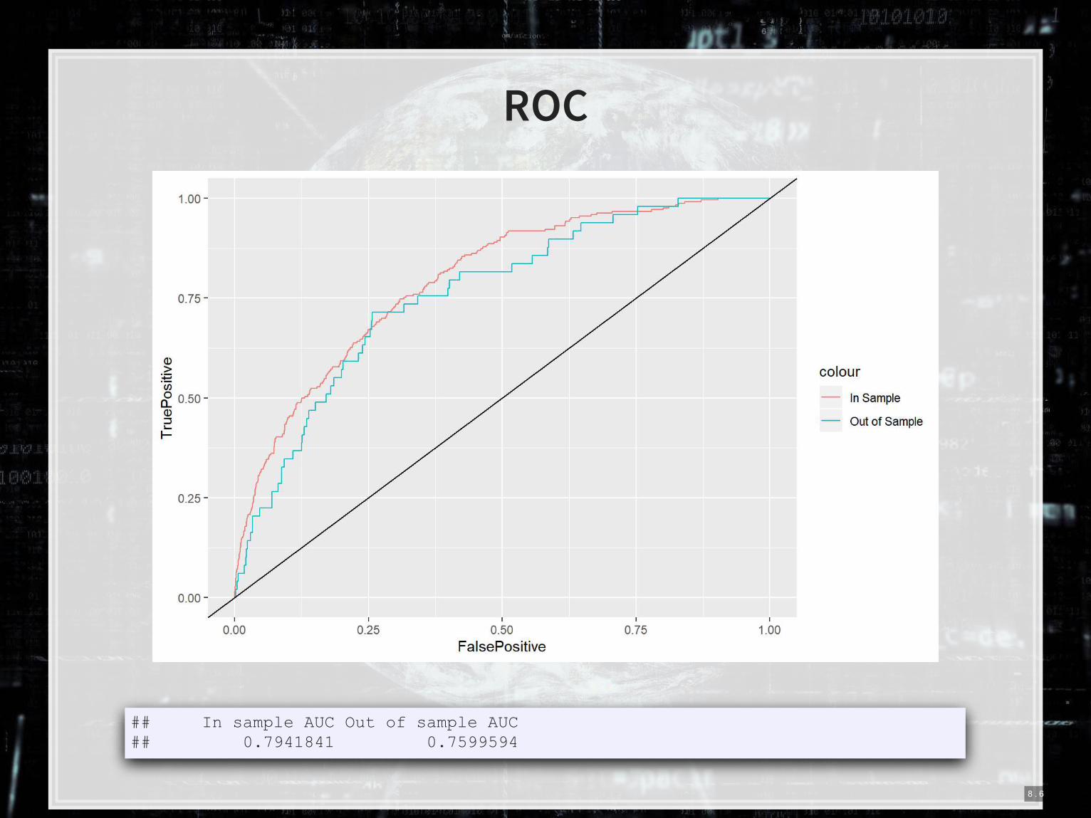
ROC
## In sample AUC Out of sample AUC ## 0.7941841 0.7599594
8 . 6
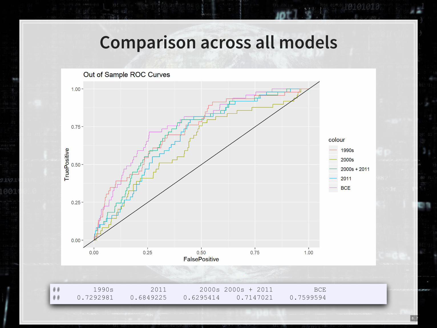
Comparison across all models
## 1990s 2011 2000s 2000s + 2011 BCE ## 0.7292981 0.6849225 0.6295414 0.7147021 0.7599594
8 . 7

Simplifying models with LASSO
9 . 1

What is LASSO?
▪ Least Absolute Shrinkage and Selection Operator
▪ Least absolute: uses an error term like
▪ Shrinkage: it will make coefficients smaller
▪ Less sensitive → less overfitting issues
▪ Selection: it will completely remove some variables
▪ Less variables → less overfitting issues
▪ Sometimes called regularization
▪ means 1 dimensional distance, i.e.,
▪ This is how we can, in theory, put more variables in our model than
data points
Great if you have way too many inputs in your model
9 . 2

▪ Add an additional penalty
term that is increasing in the
absolute value of each
▪ Incentivizes lower s,
shrinking them
▪ The selection is part is
explainable geometrically
How does it work?
9 . 3

Why use it?
1. We have a preference for simpler models
2. Some problems are naturally very complex
▪ Many linkages between different theoretical constructs
3. We don’t have a good judgment on what theories are better than
others for the problem
LASSO lets us implement all of our ideas, and then it
econometrically kicks out the ineffective ideas (model
selection)
9 . 4

Package for LASSO
▪
1. For all regression commands, they expect a y vector and an x matrix
instead of our usual y ~ x formula
▪ R has a helper function to convert a formula to a matrix:
model.matrix()
▪ Supply it the right hand side of the equation, starting with ~,
and your data
▪ It outputs the matrix x
▪ Alternatively, use as.matrix() on a data frame of your input
variables
2. It’s family argument should be specified in quotes, i.e., "binomial"
instead of binomial
glmnet
9 . 5

Ridge regression
▪ Similar to LASSO, but with an
penalty (Euclidean norm)
Elastic net regression
▪ Hybrid of LASSO and Ridge
▪ Below image by
What else can the package do?
Jared Lander
9 . 6

How to run a LASSO
▪ To run a simple LASSO model, use glmnet()
▪ Let’s LASSO the BCE model
▪ Note: the model selection can be more elegantly done using the
package,
library(glmnet) x <- model.matrix(BCE_eq, data=df[df$Test==0,])[,-1] # [,-1] to remove intercept y <- model.frame(BCE_eq, data=df[df$Test==0,])[,"AAER"] fit_LASSO <- glmnet(x=x, y=y, family = "binomial", alpha = 1 # Specifies LASSO. alpha = 0 is ridge )
useful see here for an example
9 . 7

Visualizing Lasso
plot(fit_LASSO)
9 . 8

What’s under the hood?
print(fit_LASSO)
## ## Call: glmnet(x = x, y = y, family = "binomial", alpha = 1) ## ## Df %Dev Lambda ## [1,] 0 1.312e-13 1.433e-02 ## [2,] 1 8.060e-03 1.305e-02 ## [3,] 1 1.461e-02 1.189e-02 ## [4,] 1 1.995e-02 1.084e-02 ## [5,] 2 2.471e-02 9.874e-03 ## [6,] 2 3.219e-02 8.997e-03 ## [7,] 2 3.845e-02 8.197e-03 ## [8,] 2 4.371e-02 7.469e-03 ## [9,] 2 4.813e-02 6.806e-03 ## [10,] 3 5.224e-02 6.201e-03 ## [11,] 3 5.591e-02 5.650e-03 ## [12,] 4 5.906e-02 5.148e-03 ## [13,] 4 6.249e-02 4.691e-03 ## [14,] 5 6.573e-02 4.274e-03 ## [15,] 7 6.894e-02 3.894e-03 ## [16,] 8 7.224e-02 3.548e-03 ## [17,] 10 7.522e-02 3.233e-03
9 . 9
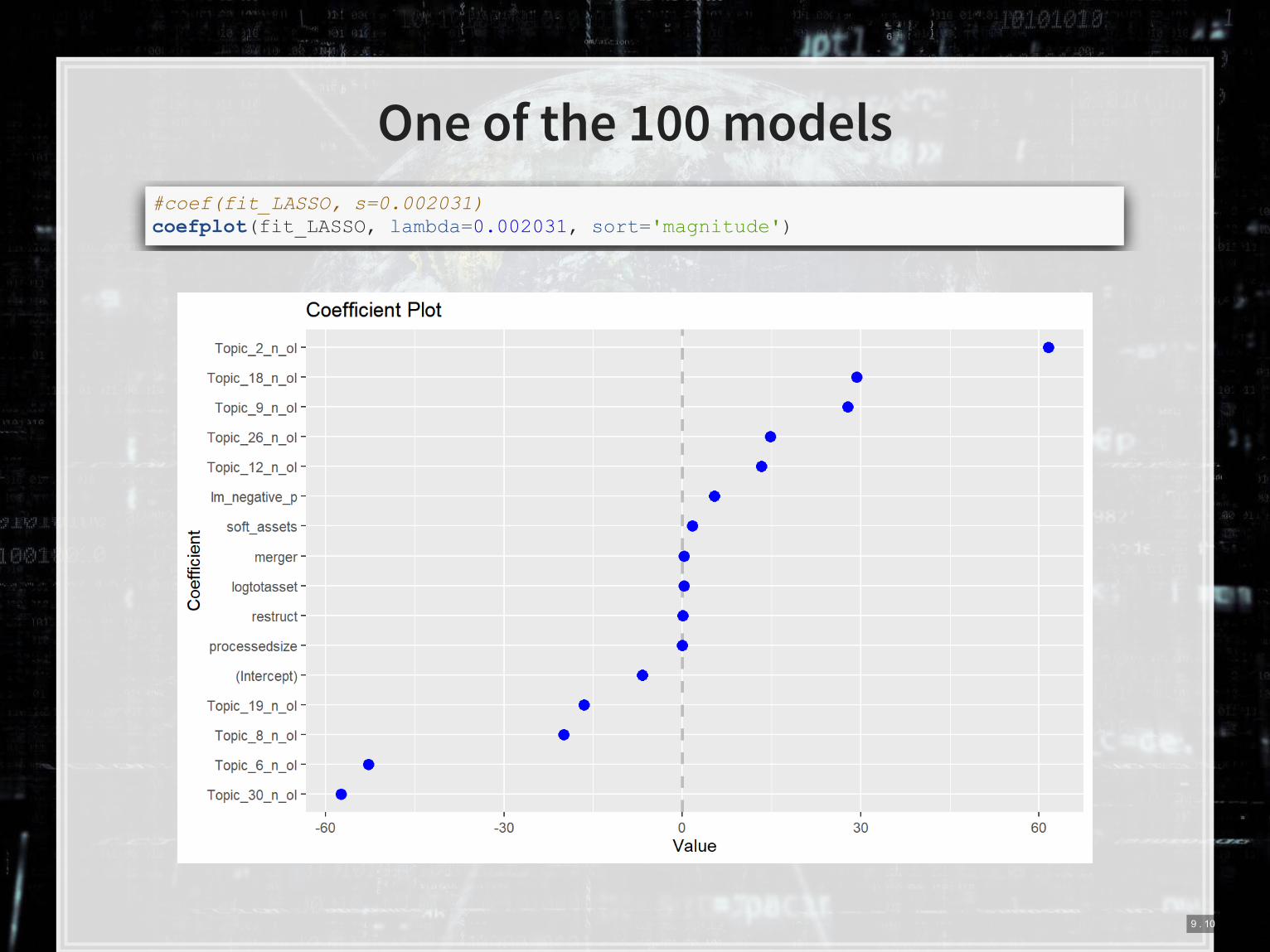
One of the 100 models
#coef(fit_LASSO, s=0.002031) coefplot(fit_LASSO, lambda=0.002031, sort='magnitude')
9 . 10
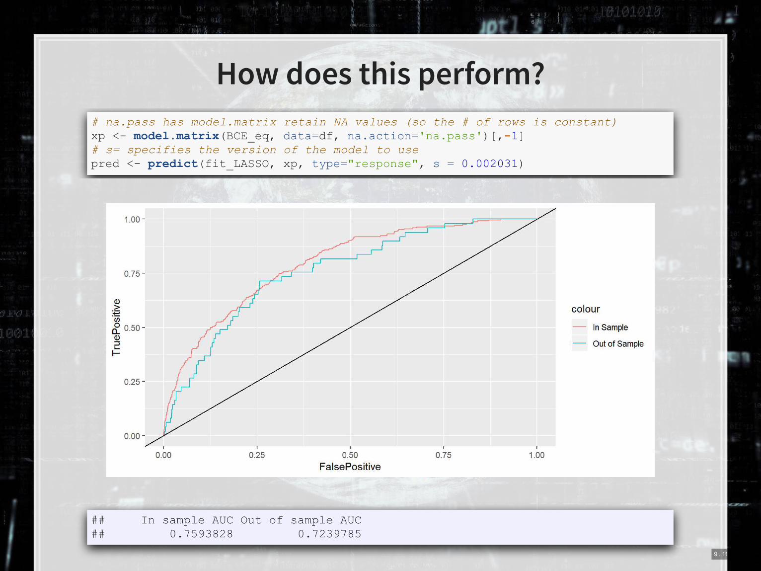
How does this perform?
# na.pass has model.matrix retain NA values (so the # of rows is constant) xp <- model.matrix(BCE_eq, data=df, na.action='na.pass')[,-1] # s= specifies the version of the model to use pred <- predict(fit_LASSO, xp, type="response", s = 0.002031)
## In sample AUC Out of sample AUC ## 0.7593828 0.7239785
9 . 11

Automating model selection
▪ LASSO seems nice, but picking between the 100 models is tough!
▪ It also contains a method of -fold cross validation (default, )
1. Randomly splits the data into groups
2. Runs the algorithm on 90% of the data ( groups)
3. Determines the best model
4. Repeat steps 2 and 3 more times
5. Uses the best overall model across all hold out samples
▪ It gives 2 model options:
▪ "lambda.min": The best performing model
▪ "lambda.1se": The simplest model within 1 standard error of
"lambda.min"
▪ This is the better choice if you are concerned about overfitting
9 . 12

Running a cross validated model
# Cross validation set.seed(697435) #for reproducibility cvfit = cv.glmnet(x=x, y=y,family = "binomial", alpha = 1, type.measure="auc")
plot(cvfit) cvfit$lambda.min
## [1] 0.001685798
cvfit$lambda.1se
## [1] 0.002684268
9 . 13
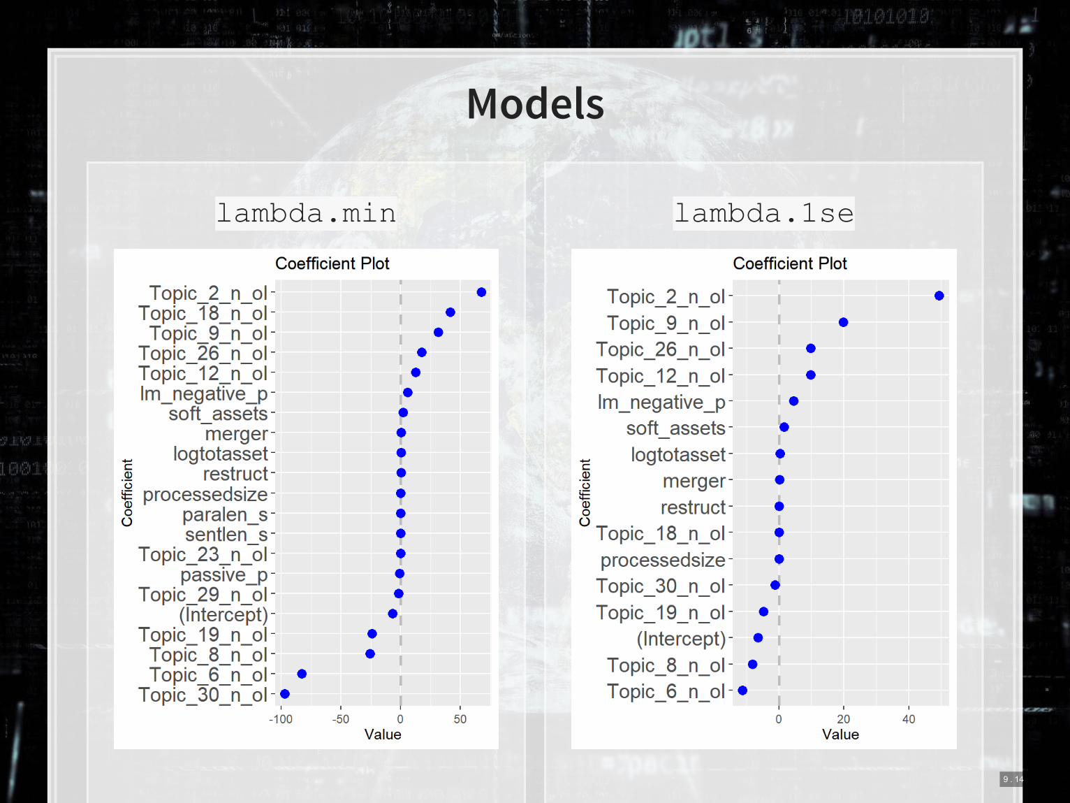
lambda.min lambda.1se
Models
9 . 14
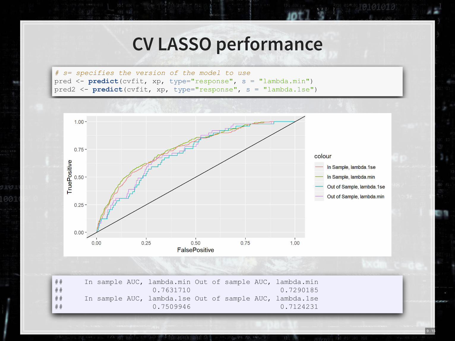
CV LASSO performance
# s= specifies the version of the model to use pred <- predict(cvfit, xp, type="response", s = "lambda.min") pred2 <- predict(cvfit, xp, type="response", s = "lambda.1se")
## In sample AUC, lambda.min Out of sample AUC, lambda.min ## 0.7631710 0.7290185 ## In sample AUC, lambda.1se Out of sample AUC, lambda.1se ## 0.7509946 0.7124231
9 . 15

Drawbacks of LASSO
1. No p-values on coefficients
▪ Simple solution – run the resulting model with
▪ Solution only if using family="gaussian":
▪ Run the lasso use the package
▪ m <- lars(x=x, y=y, type="lasso")
▪ Then test coefficients using the package
▪ covTest(m, x, y)
2. Generally worse in sample performance
3. Sometimes worse out of sample performance (short run)
▪ BUT: predictions will be more stable
glm()
lars
covTest
9 . 16

Wrap up
10 . 1

Predicting fraud
▪ What is the reason that this event or data would be useful for
prediction?
▪ I.e., how does it fit into your mental model?
▪ What if we were…
▪ Auditors?
▪ Internal auditors?
▪ Regulators?
▪ Investors?
What other data could we use to predict corporate fraud?
10 . 2

End matter
11 . 1

For next week
▪ Next week:
▪ Third assignment
▪ On binary prediction
▪ Finish by the end of next week
▪ Can be done in pairs
▪ Submit on eLearn
▪ Datacamp
▪ Practice a bit more to keep up to date
▪ Using R more will make it more natural
11 . 2

Homework 3
▪ Another question that has both forecasting and forensic flair to it
▪ Forensic: O�en these companies were doing something wrong for a
while in the past
▪ Forecasting: Predicting the actions of the firms’ investors
▪ Methods
▪ A simple logistic model from 1994
▪ A better logistic model from 2012
▪ A LASSO model including firms’ disclosure text
▪ [Optional] eXtreme Gradient Boosting (XGBoost)
Predicting class action lawsuits
11 . 3
Packages used for these slides
▪
▪
▪
▪
▪
▪
▪
▪
coefplot
glmnet
kableExtra
knitr
magrittr
revealjs
ROCR
tidyverse
11 . 4

LASSO using tidymodels
▪ There are many convenience packages in R to simplify workflows
▪ tidymodels is a collection of such packages
▪ helps process and prep data
▪ helps run models on many different backends
▪ Jared Lander gave a good talk on using tidy models,
, at DSSG
recipes
parsnip
We will use tidymodels to run a LASSO and an XGBoost
model for misreporting detection
Many ways To
Lasso
12 . 2

Data prep with recipes
library(recipes) library(parsnip) df <- read_csv("../../Data/Session_6.csv") BCEformula <- BCE_eq train <- df %>% filter(Test == 0) test <- df %>% filter(Test == 1) rec <- recipe(BCEformula, data = train) %>% step_zv(all_predictors()) %>% # Drop any variables with zero variance step_center(all_predictors()) %>% # Center all prediction variables step_scale(all_predictors()) %>% # Scale all prediction variables step_intercept() %>% # Add an intercept to the model step_num2factor(all_outcomes(), ordered = T, levels=c(0,1)) # Convert DV to fac prepped <- rec %>% prep(training=train)
12 . 3

Running a model with parsnip
# "bake" your recipe to get data ready train_baked <- bake(prepped, new_data = train) test_baked <- bake(prepped, new_data = test) # Run the model with parsnip train_model <- logistic_reg(mixture=1) %>% # mixture = 1 sets LASSO set_engine('glmnet') %>% fit(BCEformula, data = train_baked)
12 . 4

Visualizing ’s outputparsnip
# train_model$fit is the same as fit_LASSO earlier in the slides coefplot(train_model$fit, lambda=0.002031, sort='magnitude')
12 . 5

Plugging in to cross validation
▪ itself doesn’t properly support cross validation (yet)
▪ Already implemented in though, through vfold_cv()
▪ Very cumbersome to implement ourselves
▪ We can out our data and just use
parsnip
rsample
juice() cv.glmnet()rec <- recipe(BCEformula, data = train) %>% step_zv(all_predictors()) %>% # Drop any variables with zero variance step_center(all_predictors()) %>% # Center all prediction variables step_scale(all_predictors()) %>% # Scale all prediction variables step_intercept() # Add an intercept to the model prepped <- rec %>% prep(training=train) test_prepped <- rec %>% prep(training=test) # "Juice" your recipe to get data for other packages train_x <- juice(prepped, all_predictors(), composition = "dgCMatrix") train_y <- juice(prepped, all_outcomes(), composition = "matrix") test_x <- juice(test_prepped, all_predictors(), composition = "dgCMatrix") test_y <- juice(test_prepped, all_outcomes(), composition = "matrix")
12 . 6
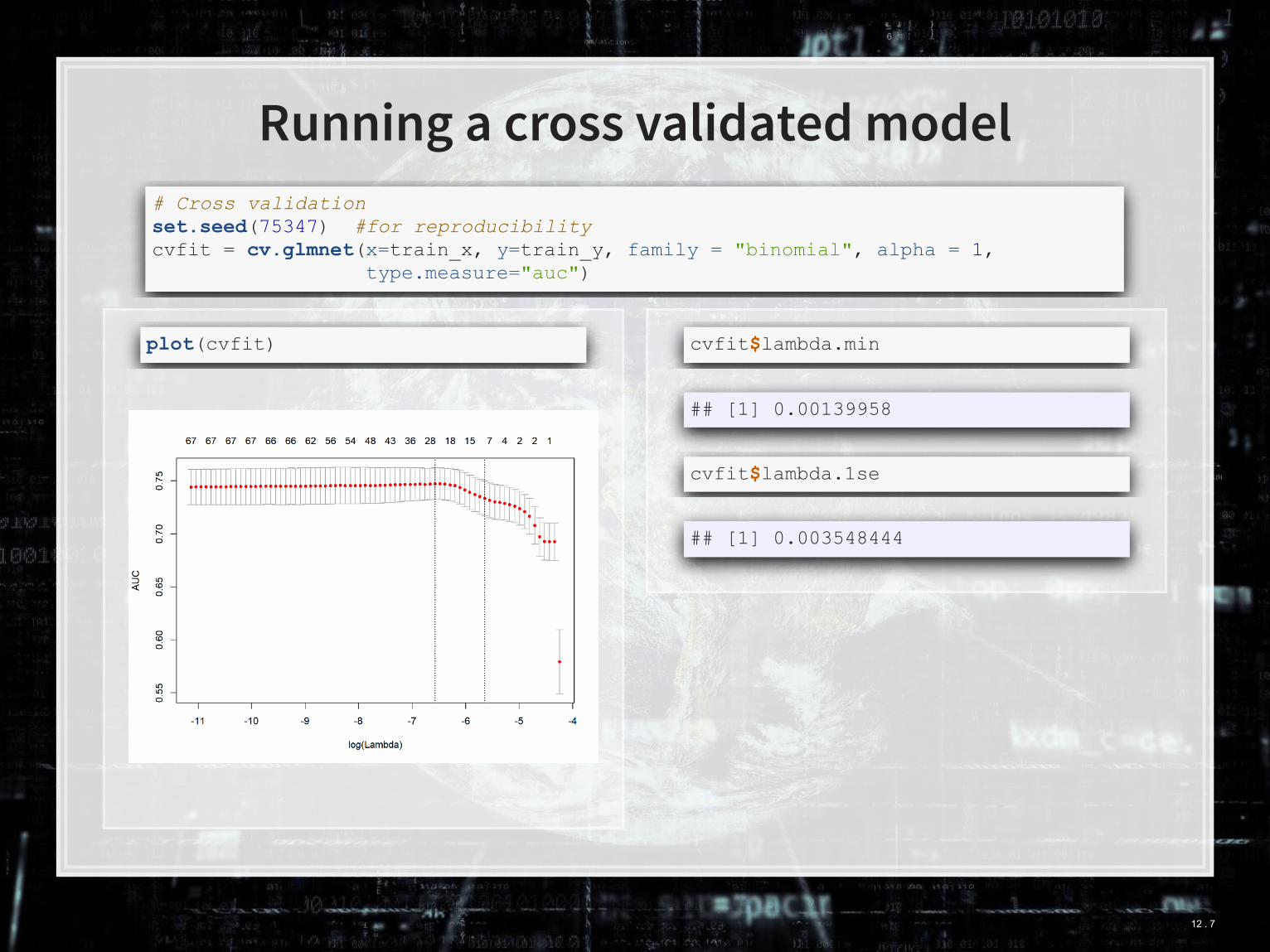
Running a cross validated model
# Cross validation set.seed(75347) #for reproducibility cvfit = cv.glmnet(x=train_x, y=train_y, family = "binomial", alpha = 1, type.measure="auc")
plot(cvfit) cvfit$lambda.min
## [1] 0.00139958
cvfit$lambda.1se
## [1] 0.003548444
12 . 7

lambda.min lambda.1se
Models
12 . 8

CV LASSO performance
## In sample AUC, lambda.min Out of sample AUC, lambda.min ## 0.7665463 0.7364834 ## In sample AUC, lambda.1se Out of sample AUC, lambda.1se ## 0.7417082 0.7028034
12 . 9

Packages used for these slides
▪
▪
▪
glmnet
parsnip
recipes
12 . 10
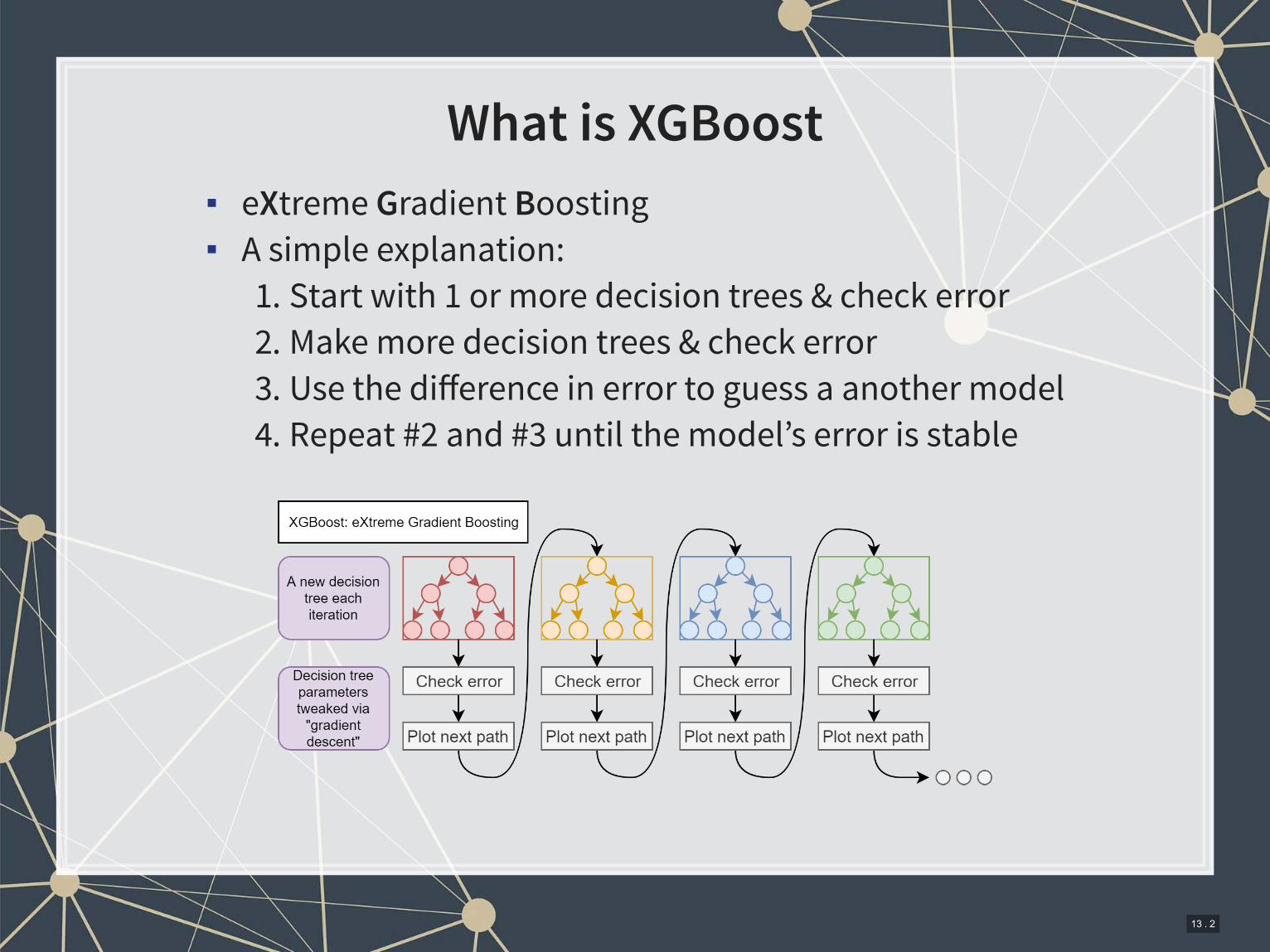
What is XGBoost
▪ eXtreme Gradient Boosting
▪ A simple explanation:
1. Start with 1 or more decision trees & check error
2. Make more decision trees & check error
3. Use the difference in error to guess a another model
4. Repeat #2 and #3 until the model’s error is stable
13 . 2

Data prep with recipes
library(recipes) library(parsnip) df <- read_csv("../../Data/Session_6.csv") BCEformula <- BCE_eq train <- df %>% filter(Test == 0) test <- df %>% filter(Test == 1) rec <- recipe(BCEformula, data = train) %>% step_zv(all_predictors()) %>% # Drop any variables with zero variance step_center(all_predictors()) %>% # Center all prediction variables step_scale(all_predictors()) %>% # Scale all prediction variables step_intercept() # Add an intercept to the model
# Juice our data prepped <- rec %>% prep(training=train) train_x <- juice(prepped, all_predictors(), composition = "dgCMatrix") train_y <- juice(prepped, all_outcomes(), composition = "matrix") test_prepped <- rec %>% prep(training=test) test_x <- juice(test_prepped, all_predictors(), composition = "dgCMatrix") test_y <- juice(test_prepped, all_outcomes(), composition = "matrix")
13 . 3

Running a cross validated model
# Cross validation set.seed(482342) #for reproducibilitylibrary(xgboost) # model setup params <- list(max_depth=10, eta=0.2, gamma=10, min_child_weight = 5, objective = "binary:logistic") # run the model xgbCV <- xgb.cv(params=params, data=train_x, label=train_y, nrounds=100, eval_metric="auc", nfold=10, stratified=TRUE)
## [1] train-auc:0.552507+0.080499 te## [2] train-auc:0.586947+0.087237 te## [3] train-auc:0.603035+0.084511 te## [4] train-auc:0.663903+0.057212 te## [5] train-auc:0.677173+0.064281 te## [6] train-auc:0.707156+0.026578 te## [7] train-auc:0.716727+0.025892 te## [8] train-auc:0.728506+0.026368 te## [9] train-auc:0.768085+0.025756 te
numTrees <- min( which( xgbCV$evaluation_log$test_auc_mea max(xgbCV$evaluation_log$test_auc_ ) ) fit4 <- xgboost(params=params, data = train_x, label = train_y, nrounds = numTrees, eval_metric="auc")
## [1] train-auc:0.500000 ## [2] train-auc:0.663489 ## [3] train-auc:0.663489 ## [4] train-auc:0.703386 ## [5] train-auc:0.703386 ## [6] train-auc:0.704123 ## [7] train-auc:0.727506 ## [8] train-auc:0.727506 ## [9] train-auc:0.727506 ## [10] train-auc:0.784639 ## [11] train-auc:0.818359 ## [12] train-auc:0.816647 ## [13] train-auc:0.851022 ## [14] train-auc:0.864434 ## [15] train-auc:0.877787 ## [16] train-auc:0.883615 ## [17] train-auc:0.885182
13 . 4
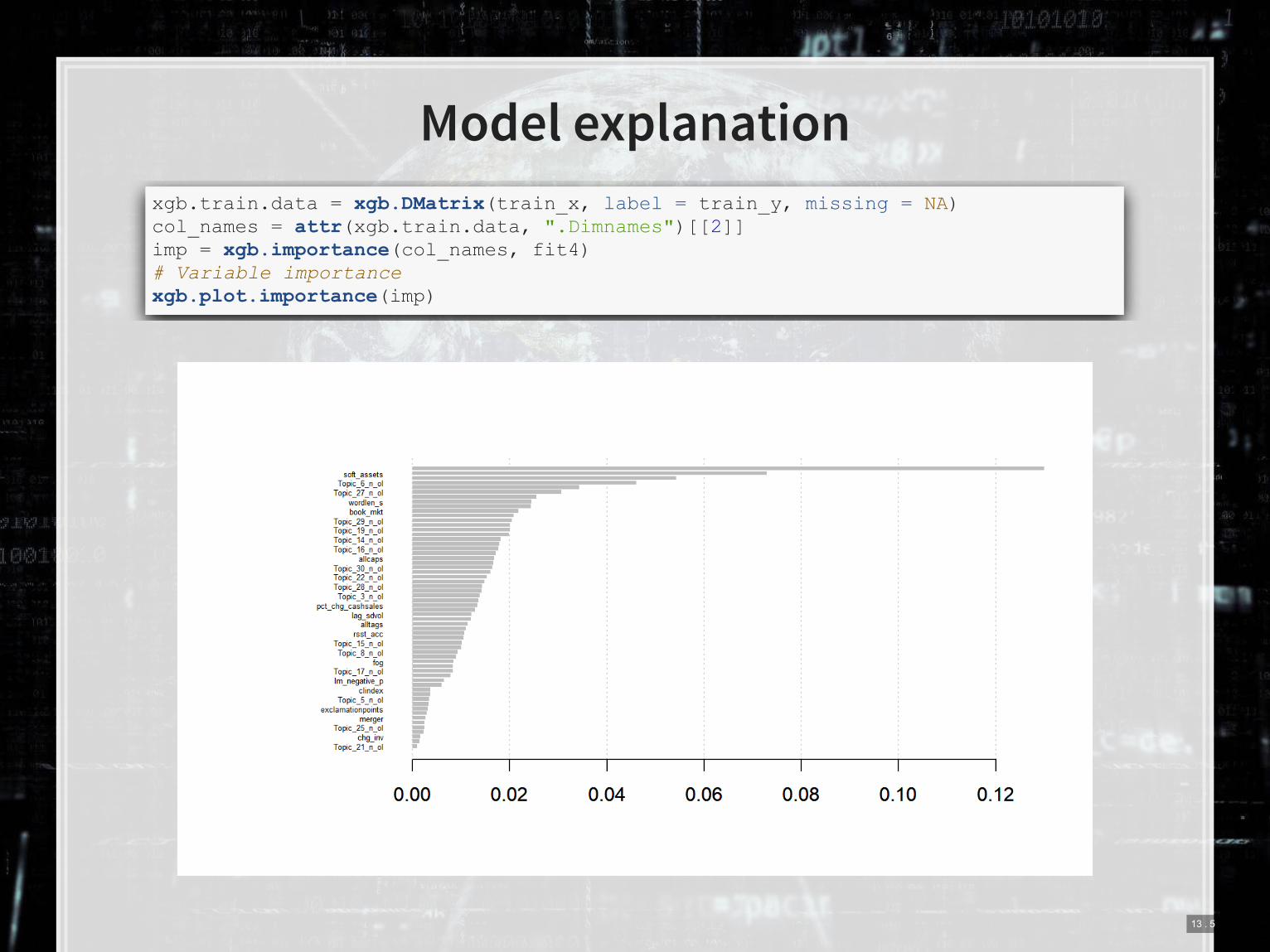
Model explanation
xgb.train.data = xgb.DMatrix(train_x, label = train_y, missing = NA) col_names = attr(xgb.train.data, ".Dimnames")[[2]] imp = xgb.importance(col_names, fit4) # Variable importance xgb.plot.importance(imp)
13 . 5

Model comparison
## 1990s 2011 2000s 2000s + 2011 ## 0.7292981 0.6849225 0.6295414 0.7147021 ## BCE LASSO, lambda.min XGBoost AUC ## 0.7599594 0.7364834 0.8083503
13 . 6

Packages used for these slides
▪
▪
▪
parsnip
recipes
xgboost
13 . 7
Recommended