Block Characterization, Modeling and STA
AccuCore Technical Training
Block Characterization, Modeling and STA
Goals
Provide a basic, usable knowledge of AccuCore. Users should gain a firm grasp of AccuCore’s: Technology Uses Application Hands-on experience
Beyond the Scope: Intricate and detailed techniques for applying AccuCore on all types of blocks (i.e. Shifter-array block versus a combinational ALU block).
- 2 -
Block Characterization, Modeling and STA
Syllabus
Introduction to AccuCore AccuCore Characterization Process AccuCore Basics Advanced Features – Characterization Lab 1 Lab 2 Lab 3 AccuCore STA Advanced Features – STA Lab 4 Summary
- 3 -
Block Characterization, Modeling and STA
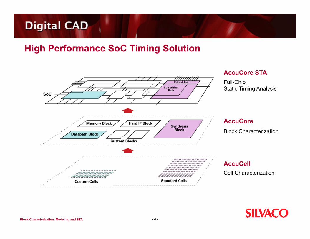
High Performance SoC Timing Solution
- 4 -
AccuCore STA Full-Chip Static Timing Analysis
AccuCore Block Characterization
AccuCell Cell Characterization
Block Characterization, Modeling and STA
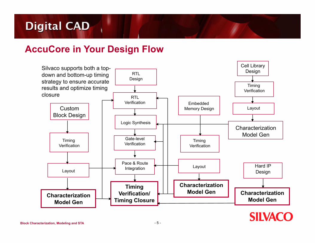
AccuCore in Your Design Flow
- 5 -
Silvaco supports both a top-down and bottom-up timing strategy to ensure accurate results and optimize timing closure
Custom Block Design
Timing Verification
Layout
Characterization Model Gen
Timing Verification/
Timing Closure
Pace & Route Integration
Gate-level Verification
Logic Synthesis
RTL Verification
RTL Design
Characterization Model Gen
Layout
Timing Verification
Embedded Memory Design
Characterization Model Gen
Hard IP Design
Characterization Model Gen
Layout
Timing Verification
Cell Library Design
Block Characterization, Modeling and STA
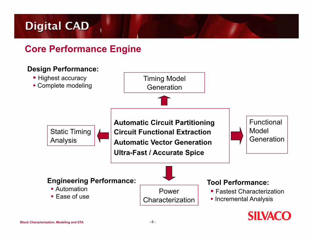
Core Performance Engine
- 6 -
Timing Model Generation
Automatic Circuit Partitioning Circuit Functional Extraction Automatic Vector Generation Ultra-Fast / Accurate Spice
Functional Model Generation
Static Timing Analysis
Power Characterization
Tool Performance: Fastest Characterization Incremental Analysis
Engineering Performance: Automation Ease of use
Design Performance: Highest accuracy Complete modeling
Block Characterization, Modeling and STA
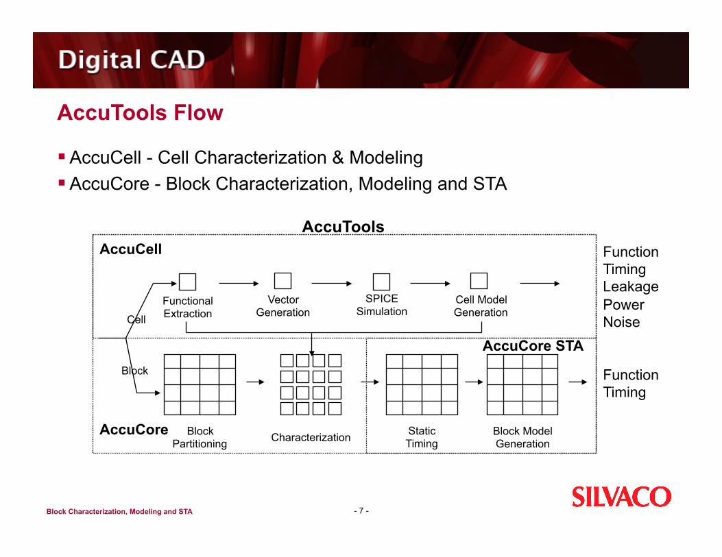
AccuTools Flow
AccuCell - Cell Characterization & Modeling AccuCore - Block Characterization, Modeling and STA
- 7 -
AccuTools
Function Timing
Functional Extraction
Vector Generation
SPICE Simulation
Cell Model Generation
Block Partitioning Characterization Static
Timing Block Model Generation
Cell
Block
Function Timing Leakage Power Noise
AccuCell
AccuCore
AccuCore STA
Block Characterization, Modeling and STA
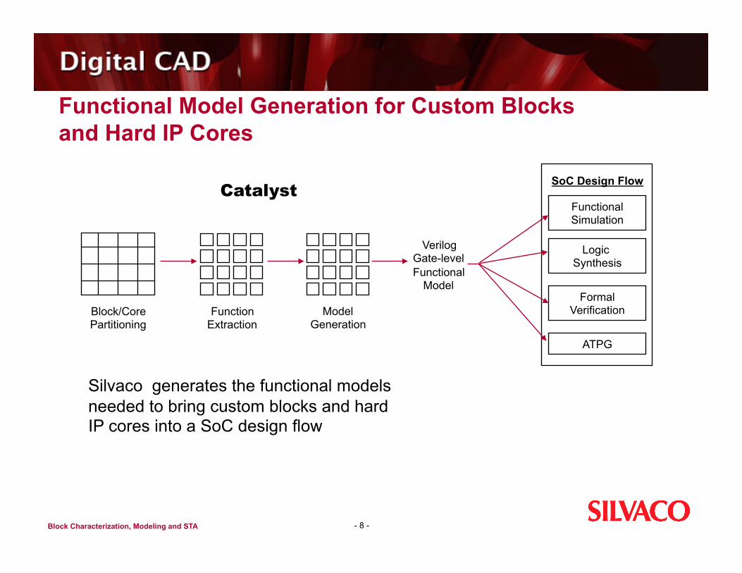
Functional Model Generation for Custom Blocks and Hard IP Cores
- 8 -
Catalyst
Block/Core Partitioning
Function Extraction
Model Generation
Verilog Gate-level Functional
Model
SoC Design Flow
Functional Simulation
Logic Synthesis
Formal Verification
ATPG
Silvaco generates the functional models needed to bring custom blocks and hard IP cores into a SoC design flow
Block Characterization, Modeling and STA
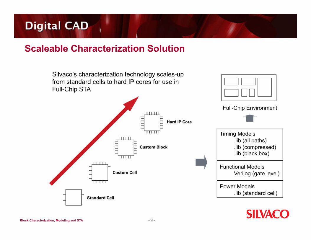
Scaleable Characterization Solution
- 9 -
Full-Chip Environment
Timing Models .lib (all paths) .lib (compressed) .lib (black box)
Functional Models Verilog (gate level)
Power Models .lib (standard cell)
Silvaco’s characterization technology scales-up from standard cells to hard IP cores for use in Full-Chip STA
Block Characterization, Modeling and STA
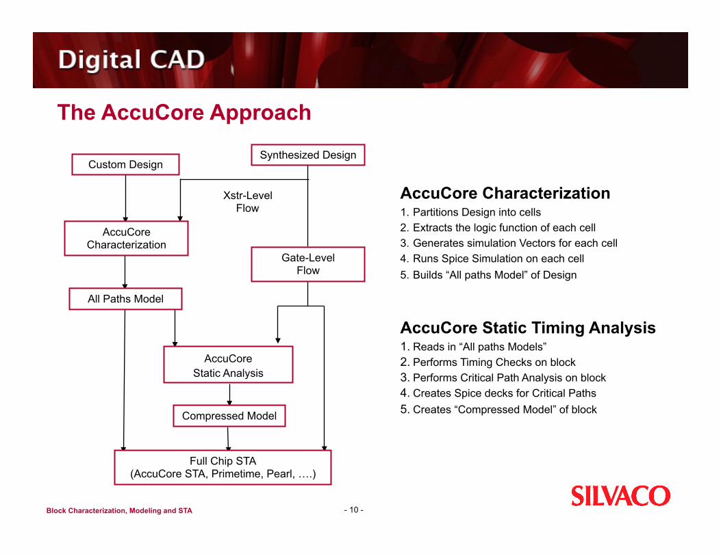
The AccuCore Approach
- 10 -
Xstr-Level Flow
Custom Design
AccuCore Characterization
All Paths Model
Full Chip STA (AccuCore STA, Primetime, Pearl, ….)
Synthesized Design
Gate-Level Flow
AccuCore Static Analysis
Compressed Model
AccuCore Characterization 1. Partitions Design into cells 2. Extracts the logic function of each cell 3. Generates simulation Vectors for each cell 4. Runs Spice Simulation on each cell 5. Builds “All paths Model” of Design
AccuCore Static Timing Analysis 1. Reads in “All paths Models” 2. Performs Timing Checks on block 3. Performs Critical Path Analysis on block 4. Creates Spice decks for Critical Paths 5. Creates “Compressed Model” of block
Block Characterization, Modeling and STA
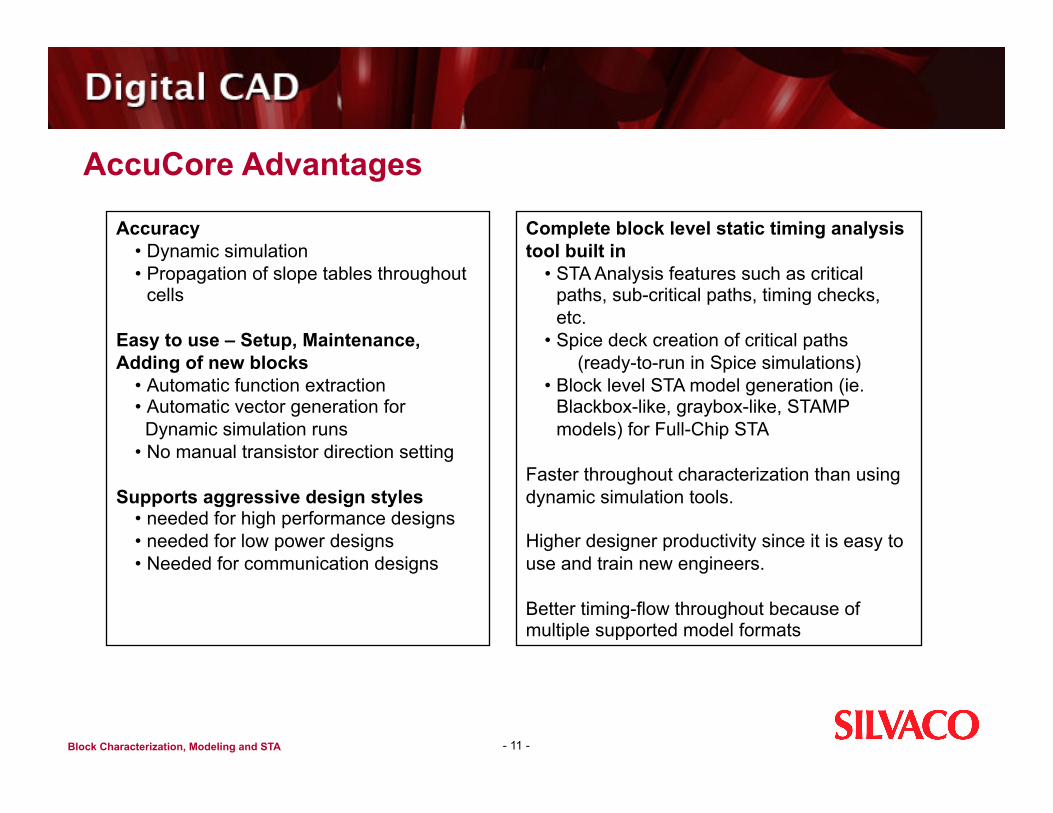
AccuCore Advantages
- 11 -
Accuracy • Dynamic simulation • Propagation of slope tables throughout
cells
Easy to use – Setup, Maintenance, Adding of new blocks
• Automatic function extraction • Automatic vector generation for Dynamic simulation runs • No manual transistor direction setting
Supports aggressive design styles • needed for high performance designs • needed for low power designs • Needed for communication designs
Complete block level static timing analysis tool built in
• STA Analysis features such as critical paths, sub-critical paths, timing checks, etc.
• Spice deck creation of critical paths (ready-to-run in Spice simulations)
• Block level STA model generation (ie. Blackbox-like, graybox-like, STAMP models) for Full-Chip STA
Faster throughout characterization than using dynamic simulation tools.
Higher designer productivity since it is easy to use and train new engineers.
Better timing-flow throughout because of multiple supported model formats
Block Characterization, Modeling and STA
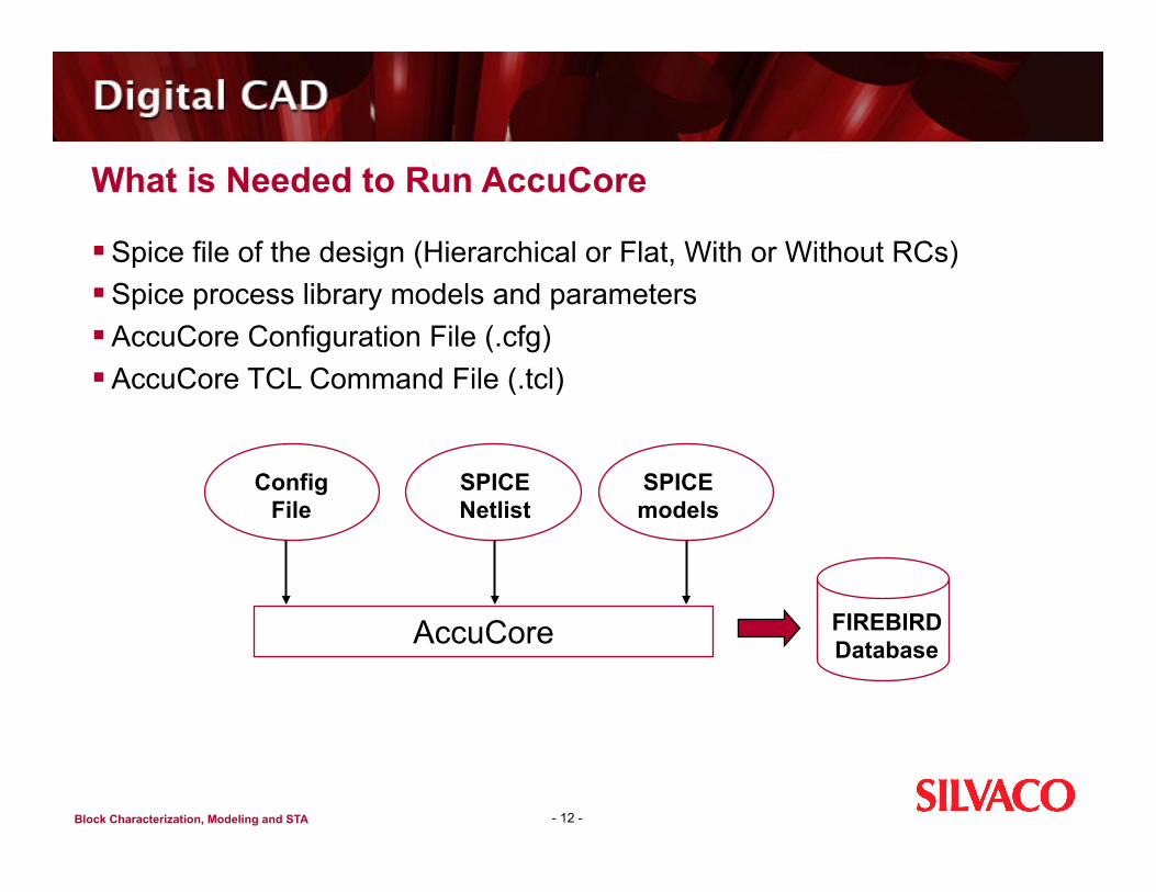
What is Needed to Run AccuCore
Spice file of the design (Hierarchical or Flat, With or Without RCs) Spice process library models and parameters AccuCore Configuration File (.cfg) AccuCore TCL Command File (.tcl)
- 12 -
Config File
SPICE Netlist
SPICE models
AccuCore FIREBIRD Database
Block Characterization, Modeling and STA
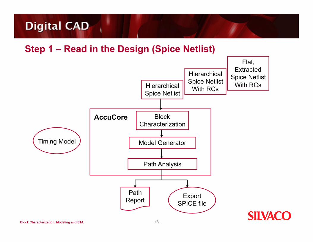
Step 1 – Read in the Design (Spice Netlist)
- 13 -
Flat, Extracted
Spice Netlist With RCs
Hierarchical Spice Netlist
With RCs Hierarchical Spice Netlist
AccuCore Block Characterization
Model Generator
Path Analysis
Export SPICE file
Path Report
Timing Model
Block Characterization, Modeling and STA
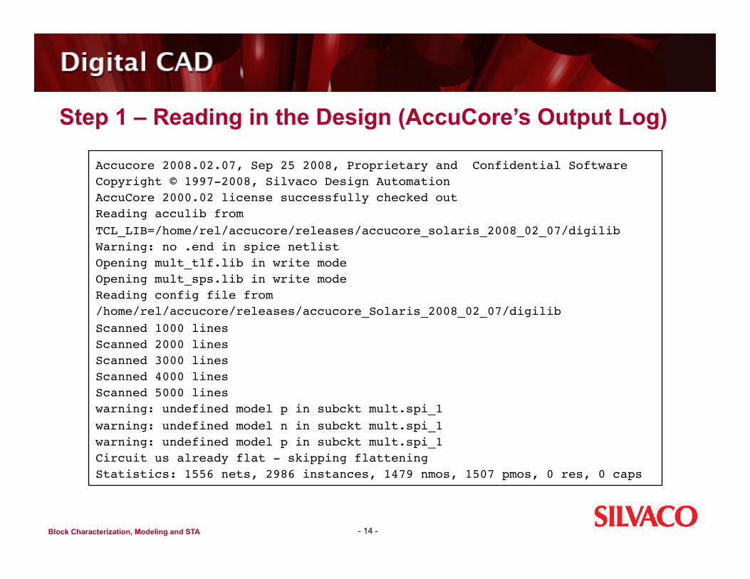
Step 1 – Reading in the Design (AccuCore’s Output Log)
- 14 -
Accucore 2008.02.07, Sep 25 2008, Proprietary and Confidential Software Copyright © 1997-2008, Silvaco Design Automation AccuCore 2000.02 license successfully checked out Reading acculib from TCL_LIB=/home/rel/accucore/releases/accucore_solaris_2008_02_07/digilib Warning: no .end in spice netlist Opening mult_tlf.lib in write mode Opening mult_sps.lib in write mode Reading config file from /home/rel/accucore/releases/accucore_Solaris_2008_02_07/digilib Scanned 1000 lines Scanned 2000 lines Scanned 3000 lines Scanned 4000 lines Scanned 5000 lines warning: undefined model p in subckt mult.spi_1 warning: undefined model n in subckt mult.spi_1 warning: undefined model p in subckt mult.spi_1 Circuit us already flat - skipping flattening Statistics: 1556 nets, 2986 instances, 1479 nmos, 1507 pmos, 0 res, 0 caps
Block Characterization, Modeling and STA
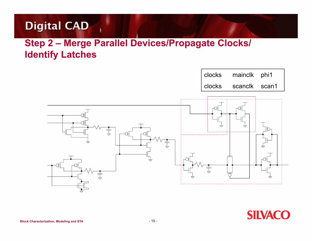
Step 2 – Merge Parallel Devices/Propagate Clocks/Identify Latches
- 15 -
clocks mainclk phi1
clocks scanclk scan1
Block Characterization, Modeling and STA
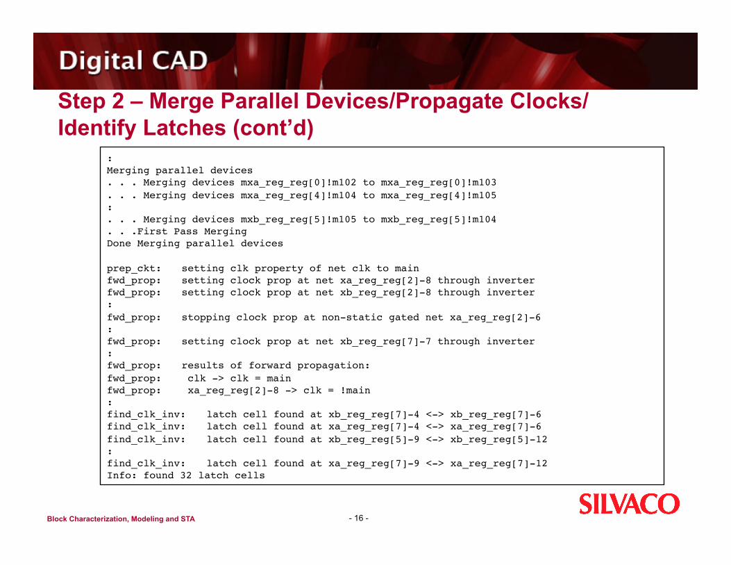
Step 2 – Merge Parallel Devices/Propagate Clocks/Identify Latches (cont’d)
- 16 -
: Merging parallel devices . . . Merging devices mxa_reg_reg[0]!m102 to mxa_reg_reg[0]!m103 . . . Merging devices mxa_reg_reg[4]!m104 to mxa_reg_reg[4]!m105 : . . . Merging devices mxb_reg_reg[5]!m105 to mxb_reg_reg[5]!m104 . . .First Pass Merging Done Merging parallel devices
prep_ckt: setting clk property of net clk to main fwd_prop: setting clock prop at net xa_reg_reg[2]-8 through inverter fwd_prop: setting clock prop at net xb_reg_reg[2]-8 through inverter : fwd_prop: stopping clock prop at non-static gated net xa_reg_reg[2]-6 : fwd_prop: setting clock prop at net xb_reg_reg[7]-7 through inverter : fwd_prop: results of forward propagation: fwd_prop: clk -> clk = main fwd_prop: xa_reg_reg[2]-8 -> clk = !main : find_clk_inv: latch cell found at xb_reg_reg[7]-4 <-> xb_reg_reg[7]-6 find_clk_inv: latch cell found at xa_reg_reg[7]-4 <-> xa_reg_reg[7]-6 find_clk_inv: latch cell found at xb_reg_reg[5]-9 <-> xb_reg_reg[5]-12 : find_clk_inv: latch cell found at xa_reg_reg[7]-9 <-> xa_reg_reg[7]-12 Info: found 32 latch cells
Block Characterization, Modeling and STA
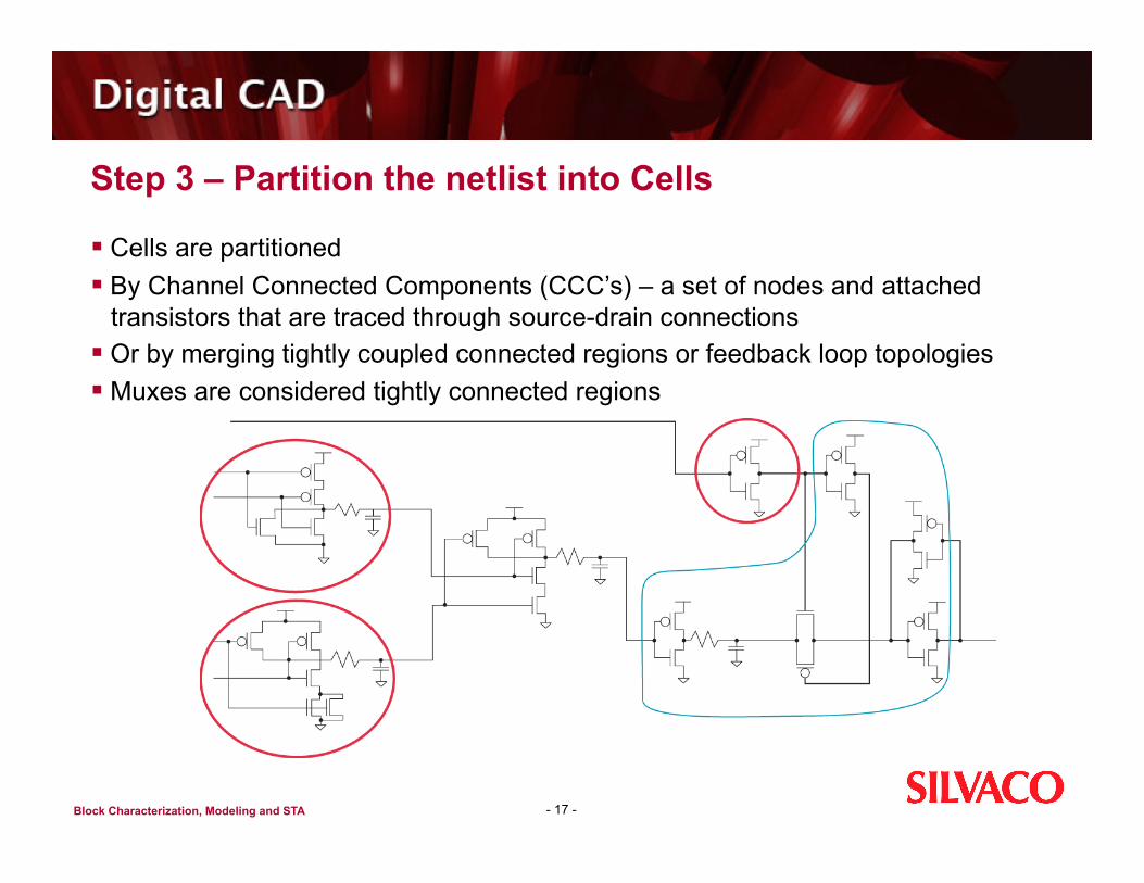
Step 3 – Partition the netlist into Cells
Cells are partitioned By Channel Connected Components (CCC’s) – a set of nodes and attached
transistors that are traced through source-drain connections Or by merging tightly coupled connected regions or feedback loop topologies Muxes are considered tightly connected regions
- 17 -
Block Characterization, Modeling and STA
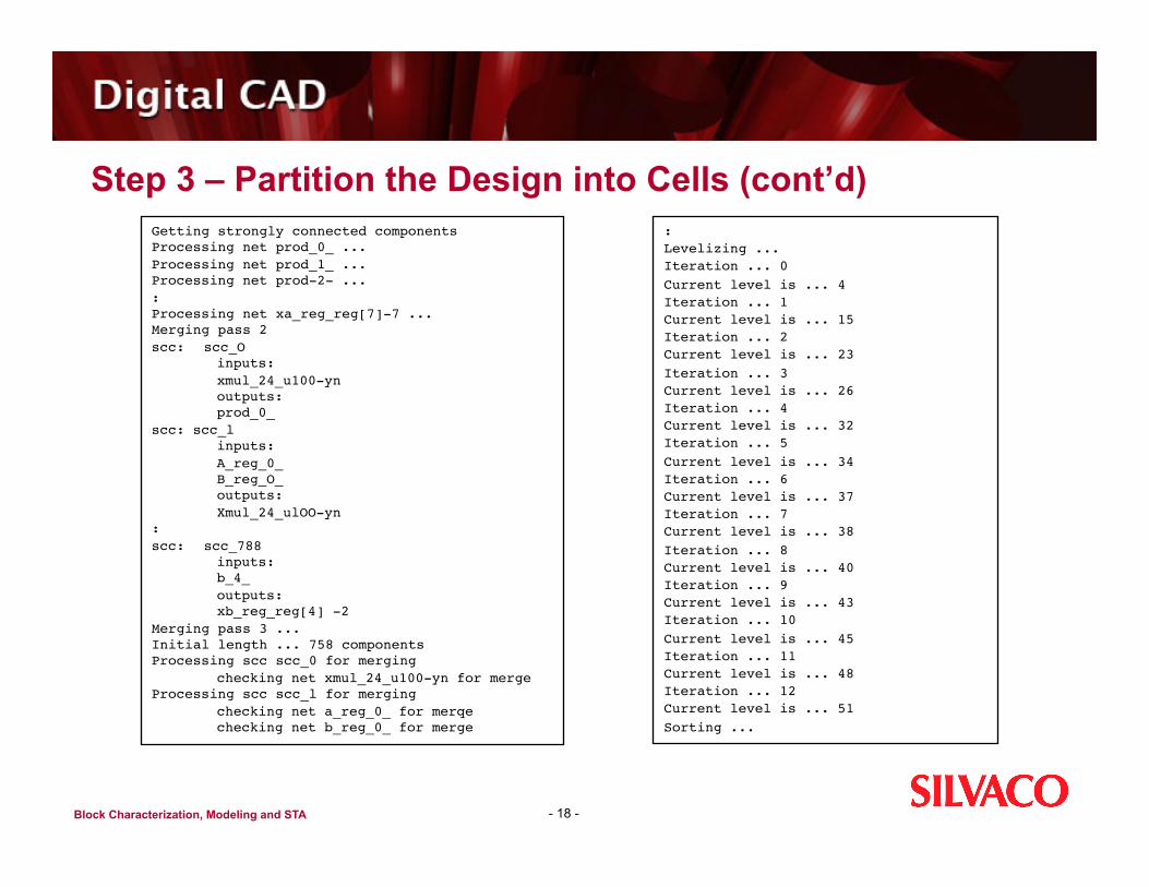
Step 3 – Partition the Design into Cells (cont’d)
- 18 -
Getting strongly connected components Processing net prod_0_ ... Processing net prod_1_ ... Processing net prod‑2‑ ... : Processing net xa_reg_reg[7]-7 ... Merging pass 2 scc: scc_O inputs: xmul_24_u100-yn outputs: prod_0_ scc: scc_l inputs: A_reg_0_ B_reg_O_ outputs: Xmul_24_ulOO-yn : scc: scc_788 inputs: b_4_ outputs: xb_reg_reg[4] ‑2 Merging pass 3 ... Initial length ... 758 components Processing scc scc_0 for merging checking net xmul_24_u100-yn for merge Processing scc scc_l for merging checking net a_reg_0_ for merqe checking net b_reg_0_ for merge
: Levelizing ... Iteration ... 0 Current level is ... 4 Iteration ... 1 Current level is ... 15 Iteration ... 2 Current level is ... 23 Iteration ... 3 Current level is ... 26 Iteration ... 4 Current level is ... 32 Iteration ... 5 Current level is ... 34 Iteration ... 6 Current level is ... 37 Iteration ... 7 Current level is ... 38 Iteration ... 8 Current level is ... 40 Iteration ... 9 Current level is ... 43 Iteration ... 10 Current level is ... 45 Iteration ... 11 Current level is ... 48 Iteration ... 12 Current level is ... 51 Sorting ...
Block Characterization, Modeling and STA
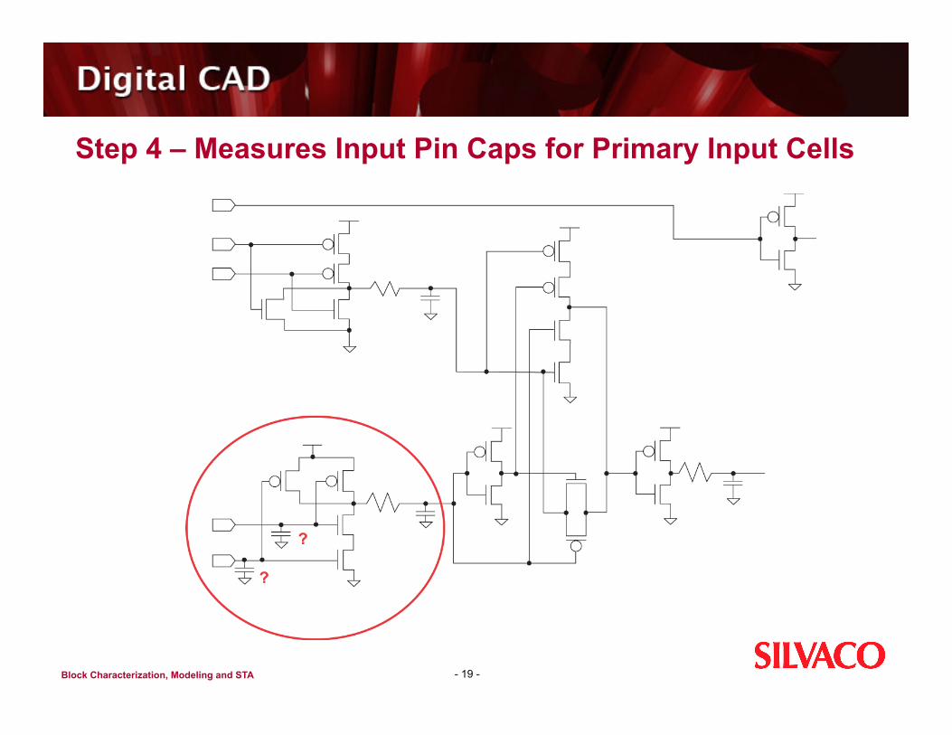
Step 4 – Measures Input Pin Caps for Primary Input Cells
- 19 -
Block Characterization, Modeling and STA
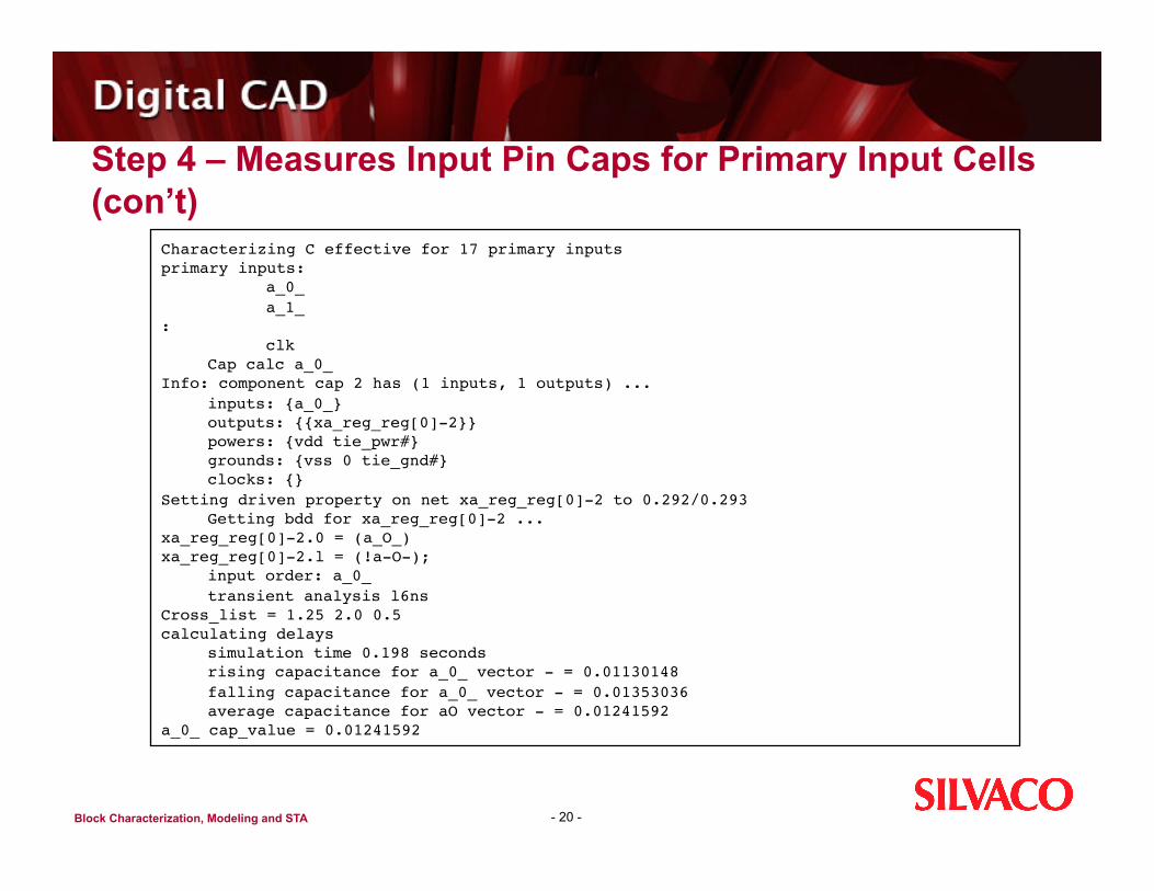
Step 4 – Measures Input Pin Caps for Primary Input Cells (con’t)
- 20 -
Characterizing C effective for 17 primary inputs primary inputs: a_0_ a_1_ : clk Cap calc a_0_ Info: component cap 2 has (1 inputs, 1 outputs) ... inputs: {a_0_} outputs: {{xa_reg_reg[0]-2}} powers: {vdd tie_pwr#} grounds: {vss 0 tie_gnd#} clocks: {} Setting driven property on net xa_reg_reg[0]-2 to 0.292/0.293 Getting bdd for xa_reg_reg[0]-2 ... xa_reg_reg[0]-2.0 = (a_O_) xa_reg_reg[0]-2.l = (!a‑O‑); input order: a_0_ transient analysis l6ns Cross_list = 1.25 2.0 0.5 calculating delays simulation time 0.198 seconds rising capacitance for a_0_ vector - = 0.01130148 falling capacitance for a_0_ vector - = 0.01353036 average capacitance for aO vector - = 0.01241592 a_0_ cap_value = 0.01241592
Block Characterization, Modeling and STA
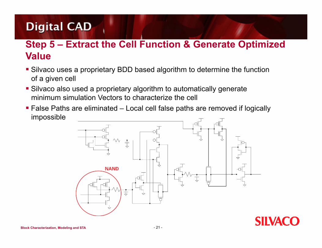
Step 5 – Extract the Cell Function & Generate Optimized Value Silvaco uses a proprietary BDD based algorithm to determine the function
of a given cell Silvaco also used a proprietary algorithm to automatically generate
minimum simulation Vectors to characterize the cell False Paths are eliminated – Local cell false paths are removed if logically
impossible
- 21 -
Block Characterization, Modeling and STA
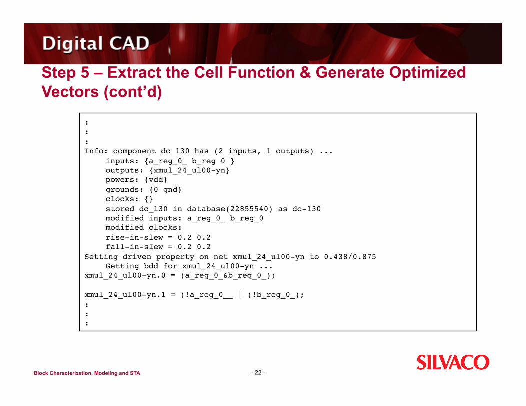
Step 5 – Extract the Cell Function & Generate Optimized Vectors (cont’d)
- 22 -
: : : Info: component dc 130 has (2 inputs, 1 outputs) ... inputs: {a_reg_0_ b_reg 0 } outputs: {xmul_24_ul00-yn} powers: {vdd} grounds: {0 gnd} clocks: {} stored dc_l30 in database(22855540) as dc‑130 modified inputs: a_reg_0_ b_reg_0 modified clocks: rise‑in‑slew = 0.2 0.2 fall‑in‑slew = 0.2 0.2 Setting driven property on net xmul_24_ul00-yn to 0.438/0.875 Getting bdd for xmul_24_ul00-yn ... xmul_24_ul00-yn.0 = (a_reg_0_&b_req_0_);
xmul_24_ul00-yn.1 = (!a_reg_0__ | (!b_reg_0_); : : :
Block Characterization, Modeling and STA
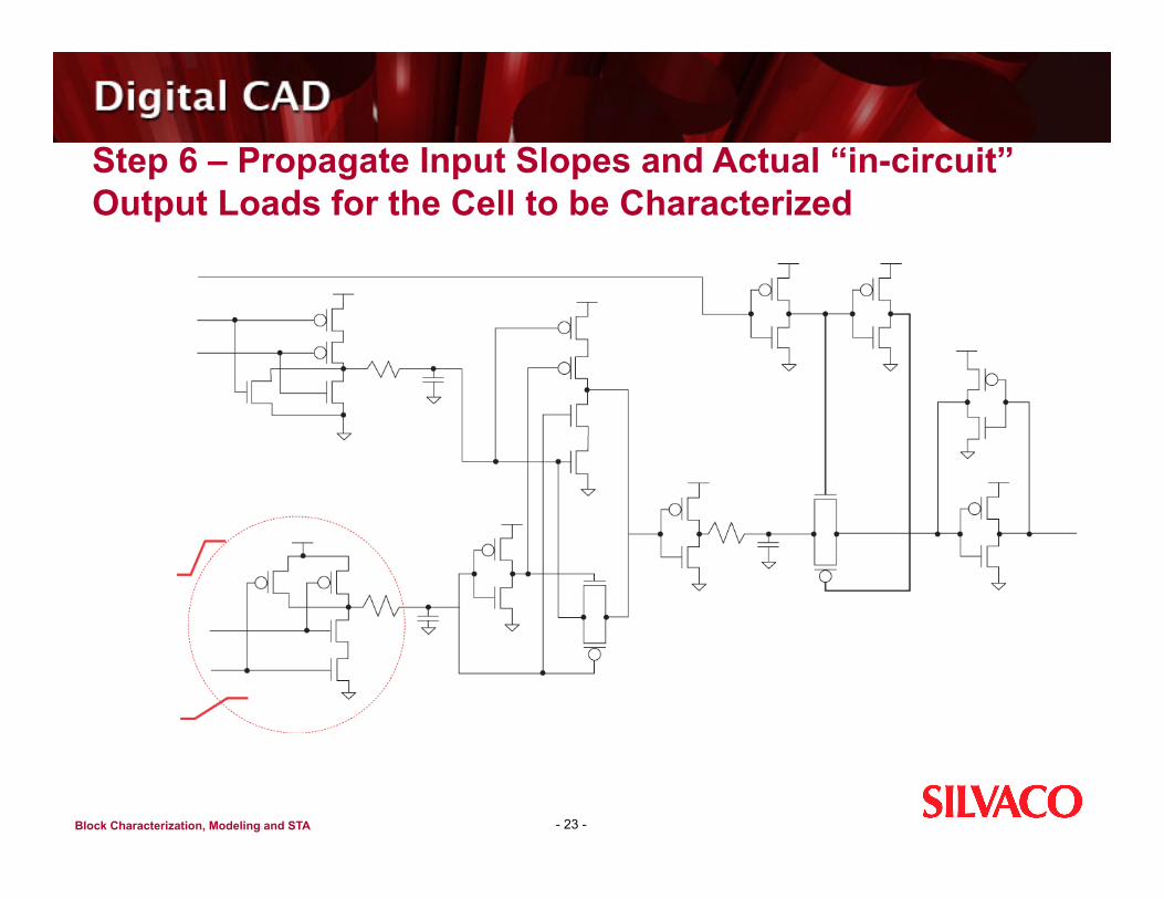
Step 6 – Propagate Input Slopes and Actual “in-circuit” Output Loads for the Cell to be Characterized
- 23 -
Block Characterization, Modeling and STA
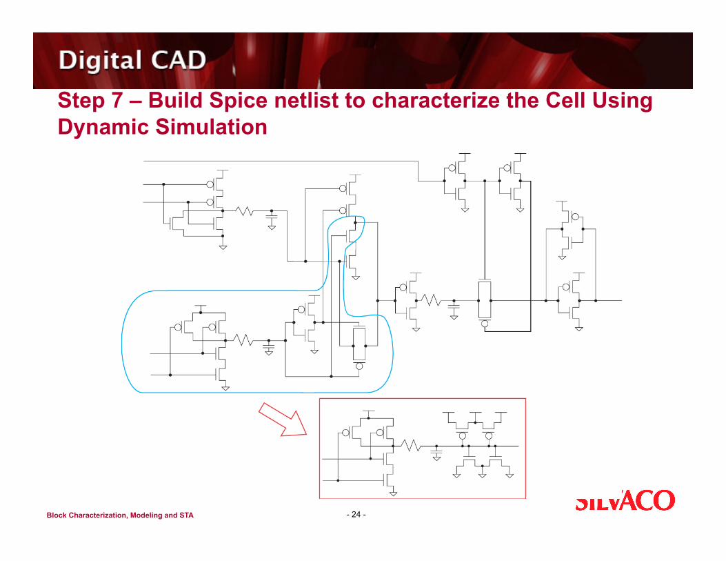
Step 7 – Build Spice netlist to characterize the Cell Using Dynamic Simulation
- 24 -
Block Characterization, Modeling and STA
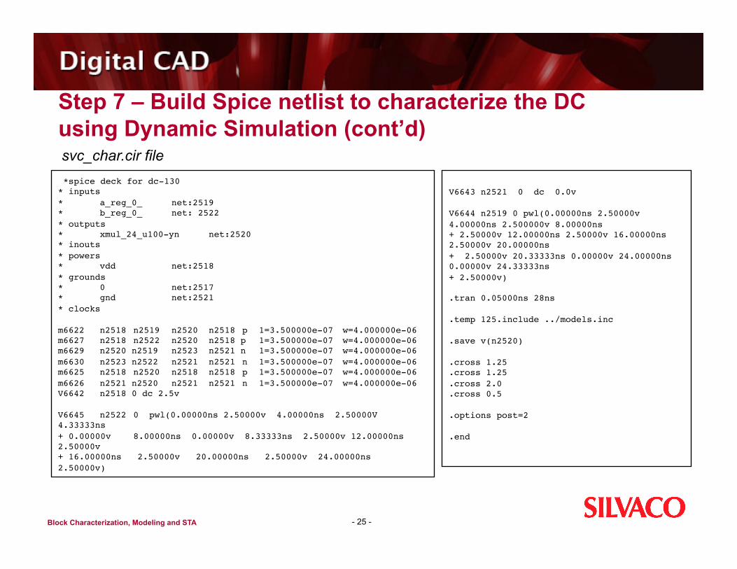
Step 7 – Build Spice netlist to characterize the DC using Dynamic Simulation (cont’d)
- 25 -
svc_char.cir file *spice deck for dc‑130 * inputs * a_reg_0_ net:2519 * b_reg_0_ net: 2522 * outputs * xmul_24_u100-yn net:2520 * inouts * powers * vdd net:2518 * grounds * 0 net:2517 * gnd net:2521 * clocks
m6622 n2518 n2519 n2520 n2518 p 1=3.500000e-07 w=4.000000e-06 m6627 n2518 n2522 n2520 n2518 p 1=3.500000e-07 w=4.000000e-06 m6629 n2520 n2519 n2523 n2521 n 1=3.500000e-07 w=4.000000e-06 m6630 n2523 n2522 n2521 n2521 n 1=3.500000e-07 w=4.000000e-06 m6625 n2518 n2520 n2518 n2518 p 1=3.500000e-07 w=4.000000e-06 m6626 n2521 n2520 n2521 n2521 n 1=3.500000e-07 w=4.000000e-06 V6642 n2518 0 dc 2.5v
V6645 n2522 0 pwl(0.00000ns 2.50000v 4.00000ns 2.50000V 4.33333ns + 0.00000v 8.00000ns 0.00000v 8.33333ns 2.50000v 12.00000ns 2.50000v + 16.00000ns 2.50000v 20.00000ns 2.50000v 24.00000ns 2.50000v)
V6643 n2521 0 dc 0.0v
V6644 n2519 0 pwl(0.00000ns 2.50000v 4.00000ns 2.500000v 8.00000ns + 2.50000v 12.00000ns 2.50000v 16.00000ns 2.50000v 20.00000ns + 2.50000v 20.33333ns 0.00000v 24.00000ns 0.00000v 24.33333ns + 2.50000v)
.tran 0.05000ns 28ns
.temp 125.include ../models.inc
.save v(n2520)
.cross 1.25
.cross 1.25
.cross 2.0
.cross 0.5
.options post=2
.end
Block Characterization, Modeling and STA
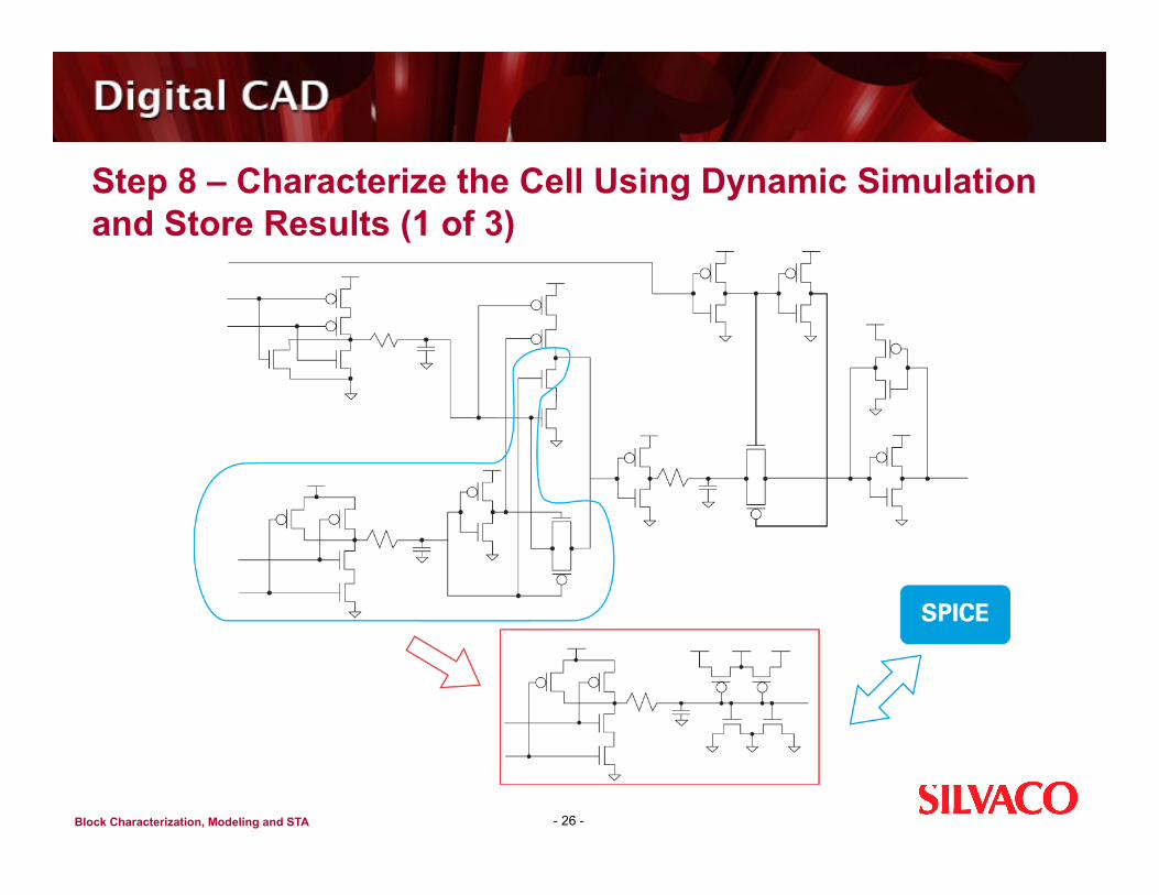
Step 8 – Characterize the Cell Using Dynamic Simulation and Store Results (1 of 3)
- 26 -
Block Characterization, Modeling and STA
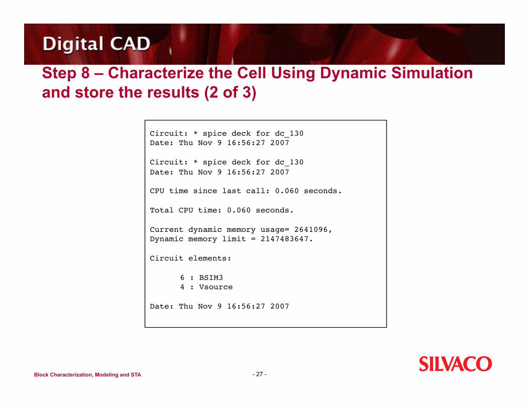
Step 8 – Characterize the Cell Using Dynamic Simulation and store the results (2 of 3)
- 27 -
Circuit: * spice deck for dc_130 Date: Thu Nov 9 16:56:27 2007
Circuit: * spice deck for dc_130 Date: Thu Nov 9 16:56:27 2007
CPU time since last call: 0.060 seconds.
Total CPU time: 0.060 seconds.
Current dynamic memory usage= 2641096, Dynamic memory limit = 2147483647.
Circuit elements:
6 : BSIM3 4 : Vsource
Date: Thu Nov 9 16:56:27 2007
Block Characterization, Modeling and STA
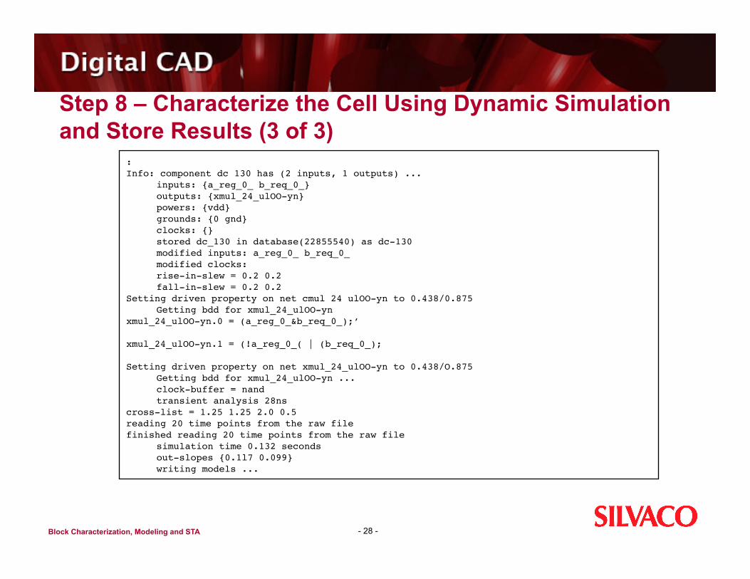
Step 8 – Characterize the Cell Using Dynamic Simulation and Store Results (3 of 3)
- 28 -
: Info: component dc 130 has (2 inputs, 1 outputs) ... inputs: {a_reg_0_ b_req_0_} outputs: {xmul_24_ulOO-yn} powers: {vdd} grounds: {0 gnd} clocks: {} stored dc_130 in database(22855540) as dc‑130 modified inputs: a_reg_0_ b_req_0_ modified clocks: rise‑in‑slew = 0.2 0.2 fall‑in‑slew = 0.2 0.2 Setting driven property on net cmul 24 ulOO‑yn to 0.438/0.875 Getting bdd for xmul_24_ulOO-yn xmul_24_ulOO-yn.0 = (a_reg_0_&b_req_0_);’
xmul_24_ulOO-yn.1 = (!a_reg_0_( | (b_req_0_);
Setting driven property on net xmul_24_ulOO-yn to 0.438/O.875 Getting bdd for xmul_24_ulOO-yn ... clock‑buffer = nand transient analysis 28ns cross‑list = 1.25 1.25 2.0 0.5 reading 20 time points from the raw file finished reading 20 time points from the raw file simulation time 0.132 seconds out‑slopes {0.1l7 0.099} writing models ...
Block Characterization, Modeling and STA
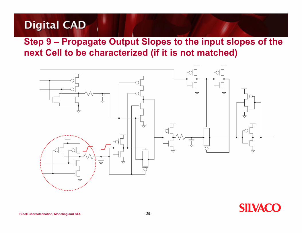
Step 9 – Propagate Output Slopes to the input slopes of the next Cell to be characterized (if it is not matched)
- 29 -
Block Characterization, Modeling and STA
AccuCore Characterization Process Summary
- 30 -
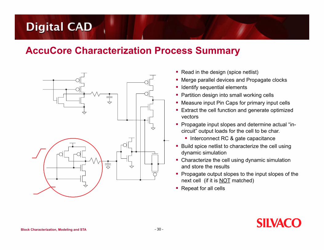
Read in the design (spice netlist) Merge parallel devices and Propagate clocks Identify sequential elements Partition design into small working cells Measure input Pin Caps for primary input cells Extract the cell function and generate optimized
vectors Propagate input slopes and determine actual “in-
circuit” output loads for the cell to be char. Interconnect RC & gate capacitance
Build spice netlist to characterize the cell using dynamic simulation
Characterize the cell using dynamic simulation and store the results
Propagate output slopes to the input slopes of the next cell (if it is NOT matched)
Repeat for all cells
Block Characterization, Modeling and STA
AccuCore “All Paths” Timing Model – Example: Liberty
- 31 -
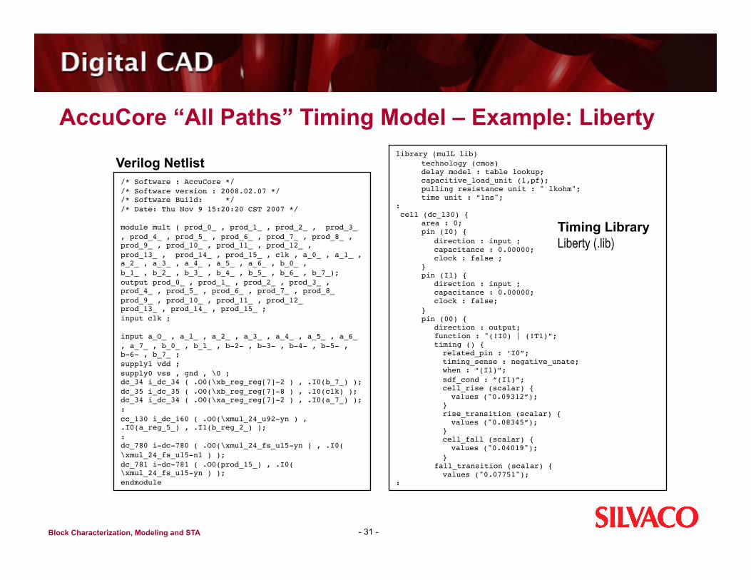
/* Software : AccuCore */ /* Software version : 2008.02.07 */ /* Software Build: */ /* Date: Thu Nov 9 15:20:20 CST 2007 */
module mult ( prod_0_ , prod_1_ , prod_2_ , prod_3_ , prod_4_ , prod_5_ , prod_6_ , prod_7_ , prod_8_ , prod_9_ , prod_10_ , prod_11_ , prod_12_ , prod_13_ , prod_14_ , prod_15_ , clk , a_0_ , a_1_ , a_2_ , a_3_ , a_4_ , a_5_ , a_6_ , b_0_ , b_1_ , b_2_ , b_3_ , b_4_ , b_5_ , b_6_ , b_7_); output prod_0_ , prod_1_ , prod_2_ , prod_3_ , prod_4_ , prod_5_ , prod_6_ , prod_7_ , prod_8_ prod_9_ , prod_10_ , prod_11_ , prod_12_ prod_13_ , prod_14_ , prod_15_ ; input clk ;
input a_O_ , a_l_ , a_2_ , a_3_ , a_4_ , a_5_ , a_6_ , a_7_ , b_0_ , b_l_ , b‑2‑ , b‑3‑ , b‑4‑ , b‑5‑ , b‑6‑ , b_7_ ; supplyl vdd ; supply0 vss , gnd , \0 ; dc_34 i_dc_34 ( .O0(\xb_reg_reg[7]-2 ) , .I0(b_7_) ); dc_35 i_dc_35 ( .O0(\xb_reg_reg[7]-8 ) , .I0(clk) ); dc_34 i_dc_34 ( .O0(\xa_reg_reg[7]-2 ) , .I0(a_7_) ); : cc_130 i_dc_160 ( .O0(\xmul_24_u92-yn ) , .I0(a_reg_5_) , .I1(b_reg_2_) ); : dc_780 i‑dc‑780 ( .O0(\xmul_24_fs_u15-yn ) , .I0( \xmul_24_fs_u15-n1 ) ); dc_781 i‑dc‑781 ( .O0(prod_15_) , .I0( \xmul_24_fs_u15-yn ) ); endmodule
library (mulL lib) technology (cmos) delay model : table lookup; capacitive_load_unit (1,pf); pulling resistance unit : " lkohm"; time unit : ”1ns"; : cell (dc_l30) { area : 0; pin (I0) { direction : input ; capacitance : 0.00000; clock : false ; } pin (I1) { direction : input ; capacitance : 0.00000; clock : false; } pin (00) { direction : output; function : "(!I0) | (!T1)”; timing () { related_pin : ‘I0”; timing_sense : negative_unate; when : “(I1)”; sdf_cond : “(I1)”; cell_rise (scalar) { values ("0.09312”); } rise_transition (scalar) { values ("0.08345”); } cell_fall (scalar) { values ("0.04019"); } fall_transition (scalar) { values ("0.07751"); :
Verilog Netlist
Timing Library Liberty (.lib)
Block Characterization, Modeling and STA
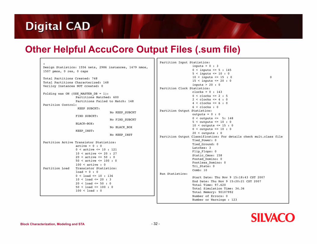
Other Helpful AccuCore Output Files (.sum file)
- 32 -
: Design Statistics: 1556 nets, 2986 instances, 1479 nmos, 1507 pmos, 0 res, 0 caps
Total Partitions Created: 748 Total Partitions Characterized: 148 Veriloy Instances NOT created: 0
Folding was ON (USE_MASTER_DB = 1): Partitions Matched: 600 Partitions Failed to Match: 148 Partition Control: KEEP SUBCKT: No KEEP_SUBCKT FIND SUBCKT: No FIND_SUBCKT BLACK‑BOX: No BLACK_BOX KEEP_INST: No KEEP_INST
Partition Active Transistor Statistics: active = 0 : 0 0 < active <= 10 : 121 10 < active <= 20 : 27 20 < active <= 50 : 0 50 < active <= 100 : 0 100 < active : 0 Partition Load Transistor Statistics: load = 0 : 0 0 < load <= 10 : 136 10 < load <= 20 : 3 20 < load <= 50 : 0 50 < load <= 100 : 0 100 < load : 0
Partition Input Statistics: inputs = 0 : 3 0 < inputs <= 5 : 145 5 < inputs <= 10 : 0 10 < inputs <= 15 : 0 0 15 < inputs <= 20 : 0 inputs > 20 : 0 Partition Clock Statistics: clocks = 0 : 143 0 < clocks <= 2 : 5 2 < clocks <= 4 : 0 4 < clocks <= 6 : 0 6 < clocks : 0 Partition Output Statistics: outputs = 0 : 0 0 < outputs <= 5: 148 5 < outputs <= 10 : 0 10 < outputs <= 15 : 0 0 < outputs <= 10 : 0 20 < outputs : 0 Partition Output Classification: For details check mult.class file Tied_Power: 0 Tied_Ground: 0 Latches: 3 Flip_Flops: 0 Static_Cmos: 158 Footed_Domino: 0 Footless_Domino: 0 Tri_State: 0 Comb: 10 Run Statistics: Start Date: Thu Nov 9 15:18:43 CST 2007 End Date: Thu Nov 9 15:20:21 CST 2007 Total Time: 97.620 Total Simulation Time: 34.36 Total Memory: 90107992 Number of Errors: 0 Number or Warnings : 123
Block Characterization, Modeling and STA
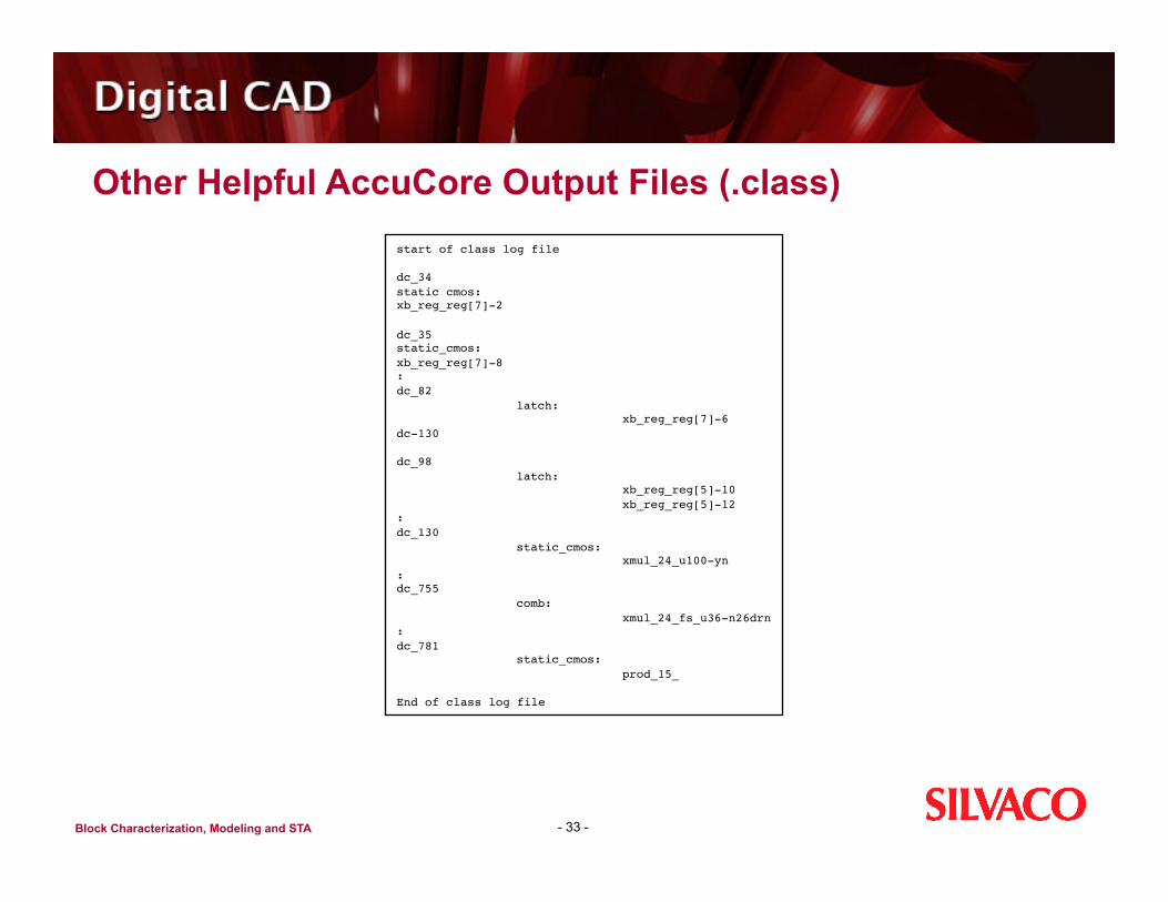
Other Helpful AccuCore Output Files (.class)
- 33 -
start of class log file
dc_34 static cmos: xb_reg_reg[7]-2
dc_35 static_cmos: xb_reg_reg[7]-8 : dc_82 latch: xb_reg_reg[7]-6 dc‑130
dc_98 latch: xb_reg_reg[5]-10 xb_reg_reg[5]-12 : dc_130 static_cmos: xmul_24_u100-yn : dc_755 comb: xmul_24_fs_u36-n26drn : dc_781 static_cmos: prod_15_
End of class log file
Block Characterization, Modeling and STA
AccuCore Basics
AccuCore Setup Running AccuCore AccuCore “All Paths” Timing Model
- 34 -
Block Characterization, Modeling and STA
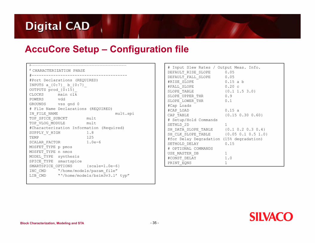
AccuCore Setup – Configuration file
- 35 -
#------------------------------------------------------------
# CHARACTERIZATION PHASE #---------------------------------------- #Port Declarations (REQUIRED) INPUTS a_{0:7}_ b_{0:7}_ OUTPUTS prod_{0:15}_ CLOCKS main clk POWERS vdd GROUNDS vss gnd 0 # File Name Declarations (REQUIRED) IN_FILE_NAME mult.spi TOP_SPICE_SUBCKT mult TOP_VLOG_MODULE mult #Characterization Information (Required) SUPPLY_V_HIGH 1.8 TEMP 125 SCALAR_FACTOR 1.0e-6 MOSFET_TYPE p pmos MOSFET_TYPE n nmos MODEL_TYPE synthesis SPICE_TYPE smartspice SMARTSPICE_OPTIONS {scale=1.0e-6} INC_CMD “/home/models/param_file” LIB_CMD “‘/home/models/bsim3v3.l’ typ”
# Input Slew Rates / Output Meas. Info. DEFAULT_RISE_SLOPE 0.05 DEFAULT_FALL_SLOPE 0.05 #RISE_SLOPE 0.15 a b #FALL_SLOPE 0.20 c SLOPE_TABLE {0.1 1.5 3.0} SLOPE_UPPER_THR 0.9 SLOPE_LOWER_THR 0.1 #Cap Loads #CAP_LOAD 0.15 a CAP_TABLE {0.15 0.30 0.60} # Setup/Hold Commands SETHLD_2D 1 SH_DATA_SLOPE_TABLE {0.1 0.2 0.3 0.4} SH_CLK_SLOPE_TABLE {0.05 0.1 0.5 1.0} #for Delay Degradation (15% degradation) SETHOLD_DELAY 0.15 # OPTIONAL COMMANDS USE_MASTER_DB 1 #CONST_DELAY 1.0 PRINT_EQNS 1
Block Characterization, Modeling and STA
AccuCore Setup – Configuration file (cont’d)
- 36 -
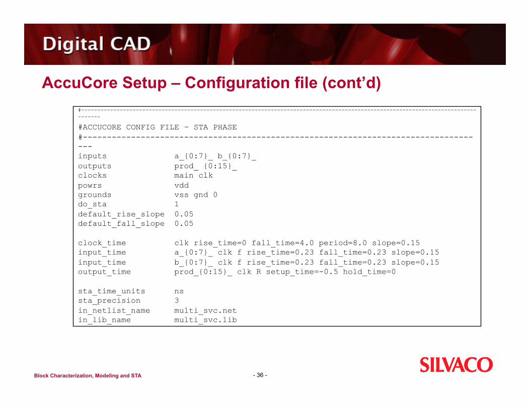
#----------------------------------------------------------------------------------------------------------------------------------
#ACCUCORE CONFIG FILE – STA PHASE #------------------------------------------------------------------------------------ inputs a_{0:7}_ b_{0:7}_ outputs prod_ {0:15}_ clocks main clk powrs vdd grounds vss gnd 0 do_sta 1 default_rise_slope 0.05 default_fall_slope 0.05
clock_time clk rise_time=0 fall_time=4.0 period=8.0 slope=0.15 input_time a_{0:7}_ clk f rise_time=0.23 fall_time=0.23 slope=0.15 input_time b_{0:7}_ clk f rise_time=0.23 fall_time=0.23 slope=0.15 output_time prod_{0:15}_ clk R setup_time=-0.5 hold_time=0
sta_time_units ns sta_precision 3 in_netlist_name multi_svc.net in_lib_name multi_svc.lib
Block Characterization, Modeling and STA
Running AccuCore
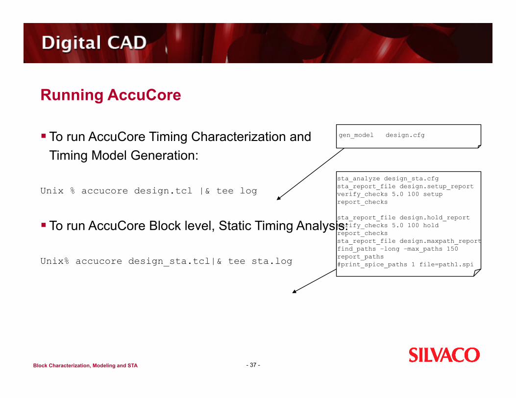
To run AccuCore Timing Characterization and Timing Model Generation:
Unix % accucore design.tcl |& tee log
To run AccuCore Block level, Static Timing Analysis: Unix% accucore design_sta.tcl|& tee sta.log
- 37 -
gen_model design.cfg
sta_analyze design_sta.cfg sta_report_file design.setup_report verify_checks 5.0 100 setup report_checks
sta_report_file design.hold_report verify_checks 5.0 100 hold report_checks sta_report_file design.maxpath_report find_paths –long –max_paths 150 report_paths #print_spice_paths 1 file=path1.spi
Block Characterization, Modeling and STA
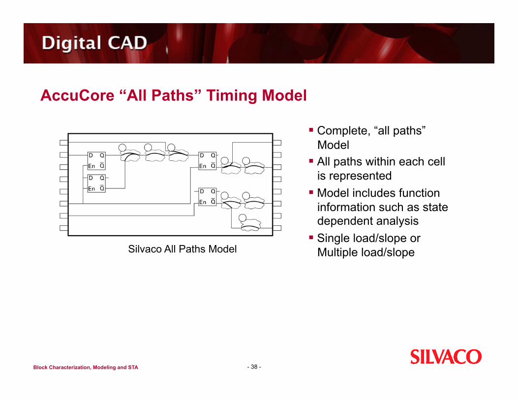
AccuCore “All Paths” Timing Model
Complete, “all paths” Model
All paths within each cell is represented
Model includes function information such as state dependent analysis
Single load/slope or Multiple load/slope
- 38 -
Silvaco All Paths Model
Block Characterization, Modeling and STA
AccuCore “All Paths” Timing Model
The model is made up of two files: 1. Verilog Netlist – contains all of the connectivity information for the
block 2. Timing Library – in Liberty “.lib Contains:
delays arc types input capacitance’s
- 39 -
Block Characterization, Modeling and STA
SmartSpice – Silvaco’s High-Performance. High-Accuracy Transistor Simulation Engine General-purpose, embedded, transistor simulation engine
100% compatible HSPICE and SPECTRE for all public models and netlist format
Performance AccuCore runs are typically 2X to 20X faster than industry standard
simulators Accuracy
Accurate the third decimal place with Industry Standard Simulators
- 40 -

LAB 1
Getting Started with AccuCore
Block Characterization, Modeling and STA
LAB 1 – Objectives
Setup a AccuCore run Run AccuCore to characterize a inverter chain circuit Familiarize yourself with AccuCore’s “all paths” model output
format
- 42 -
Block Characterization, Modeling and STA
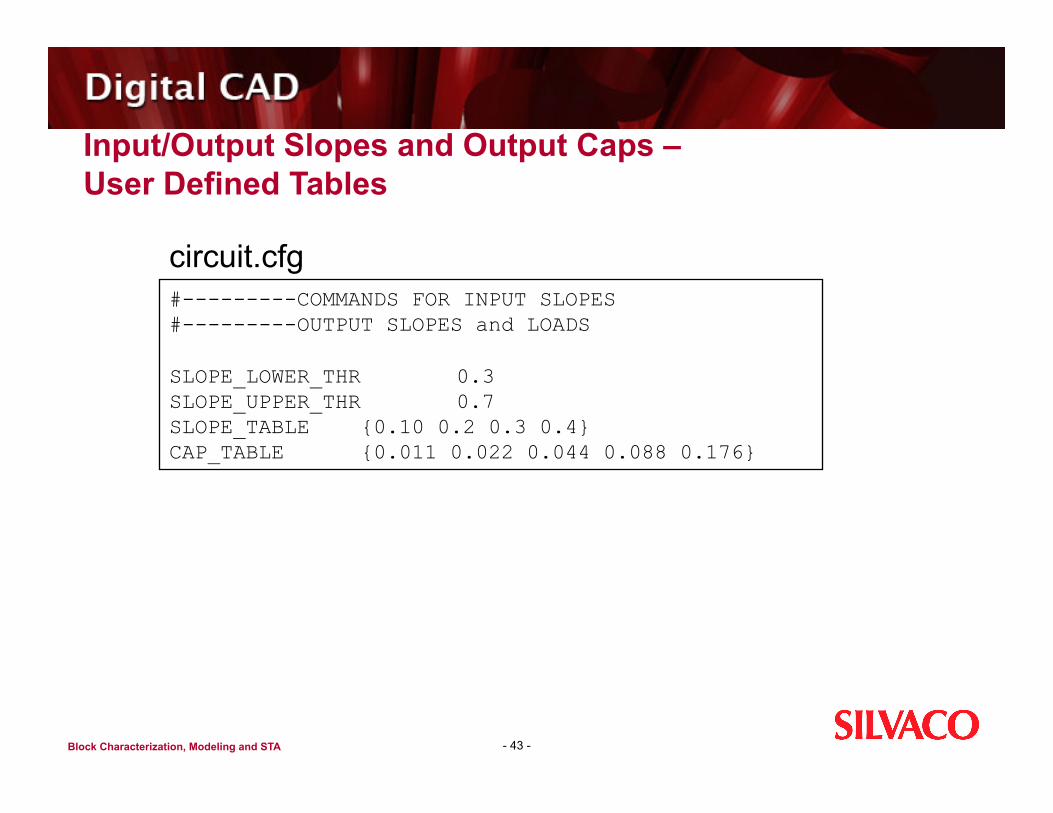
Input/Output Slopes and Output Caps – User Defined Tables
- 43 -
circuit.cfg #---------COMMANDS FOR INPUT SLOPES #---------OUTPUT SLOPES and LOADS
SLOPE_LOWER_THR 0.3 SLOPE_UPPER_THR 0.7 SLOPE_TABLE {0.10 0.2 0.3 0.4} CAP_TABLE {0.011 0.022 0.044 0.088 0.176}
Block Characterization, Modeling and STA
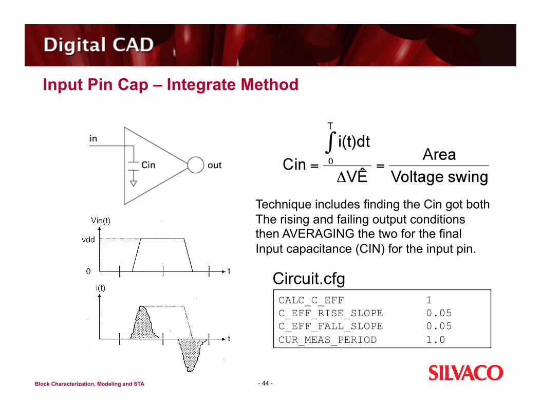
Input Pin Cap – Integrate Method
- 44 -
Circuit.cfg CALC_C_EFF 1 C_EFF_RISE_SLOPE 0.05 C_EFF_FALL_SLOPE 0.05 CUR_MEAS_PERIOD 1.0
Technique includes finding the Cin got both The rising and failing output conditions then AVERAGING the two for the final Input capacitance (CIN) for the input pin.
Block Characterization, Modeling and STA
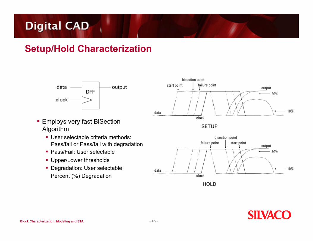
Setup/Hold Characterization
- 45 -
Employs very fast BiSection Algorithm User selectable criteria methods:
Pass/fail or Pass/fail with degradation Pass/Fail: User selectable Upper/Lower thresholds Degradation: User selectable Percent (%) Degradation
Block Characterization, Modeling and STA
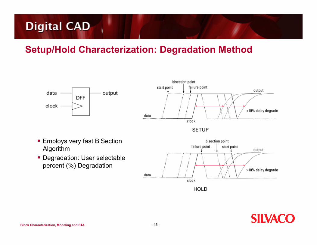
Setup/Hold Characterization: Degradation Method
- 46 -
Employs very fast BiSection Algorithm
Degradation: User selectable percent (%) Degradation
Block Characterization, Modeling and STA
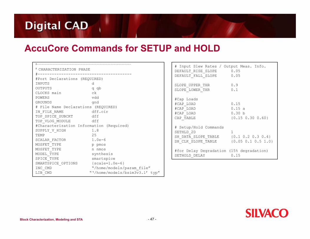
AccuCore Commands for SETUP and HOLD
- 47 -
#------------------------------------------------------------
# CHARACTERIZATION PHASE #---------------------------------------- #Port Declarations (REQUIRED) INPUTS d OUTPUTS q qb CLOCKS main ck POWERS vdd GROUNDS gnd # File Name Declarations (REQUIRED) IN_FILE_NAME dff.cir TOP_SPICE_SUBCKT dff TOP_VLOG_MODULE dff #Characterization Information (Required) SUPPLY_V_HIGH 1.8 TEMP 25 SCALAR_FACTOR 1.0e-6 MOSFET_TYPE p pmos MOSFET_TYPE n nmos MODEL_TYPE synthesis SPICE_TYPE smartspice SMARTSPICE_OPTIONS {scale=1.0e-6} INC_CMD “/home/models/param_file” LIB_CMD “‘/home/models/bsim3v3.l’ typ”
# Input Slew Rates / Output Meas. Info. DEFAULT_RISE_SLOPE 0.05 DEFAULT_FALL_SLOPE 0.05
SLOPE_UPPER_THR 0.9 SLOPE_LOWER_THR 0.1
#Cap Loads #CAP_LOAD 0.15 #CAP_LOAD 0.15 a #CAP_LOAD 0.30 b CAP_TABLE {0.15 0.30 0.60}
# Setup/Hold Commands SETHLD_2D 1 SH_DATA_SLOPE_TABLE {0.1 0.2 0.3 0.4} SH_CLK_SLOPE_TABLE {0.05 0.1 0.5 1.0}
#for Delay Degradation (15% degradation) SETHOLD_DELAY 0.15
Block Characterization, Modeling and STA
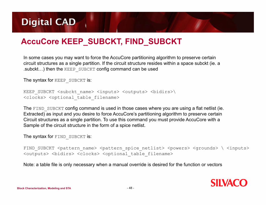
AccuCore KEEP_SUBCKT, FIND_SUBCKT
- 48 -
In some cases you may want to force the AccuCore partitioning algorithm to preserve certain circuit structures as a single partition. If the circuit structure resides within a space subckt (ie. a .subckt…) then the KEEP_SUBCKT config command can be used
The syntax for KEEP_SUBCKT is:
KEEP_SUBCKT <subckt_name> <inputs> <outputs> <bidirs>\ <clocks> <optional_table_filename>
The FIND_SUBCKT config command is used in those cases where you are using a flat netlist (ie. Extracted) as input and you desire to force AccuCore’s partitioning algorithm to preserve certain Circuit structures as a single partition. To use this command you must provide AccuCore with a Sample of the circuit structure in the form of a spice netlist.
The syntax for FIND_SUBCKT is:
FIND_SUBCKT <pattern_name> <pattern_spice_netlist> <powers> <grounds> \ <inputs> <outputs> <bidirs> <clocks> <optional_table_filename>
Note: a table file is only necessary when a manual override is desired for the function or vectors

LAB 2
- 49 -
Sequential Cells and Setup and Hold
Block Characterization, Modeling and STA
LAB 2 – Objectives
Setup AccuCore to characterize a latch circuit Run AccuCore using default setup/hold commands Run AccuCore using setup/hold Measurement commands Familiarize yourself with the equations extracted Familiarize yourself with the “all paths” model output for the latch
cell
- 50 -
LAB 3
- 51 -
KEEP_SUBCKT, FIND_SUBCKT, and Manual Overrides

Block Characterization, Modeling and STA
Lab 3 – Objectives
- 52 -
Setup AccuCore to characterize a circuit using KEEP_SUBCKT and FIND_SUBCKT
Create a Equation file (.eqn) for a circuit
Block Characterization, Modeling and STA
AccuCore Full Chip STA
Full Chip Static Gate Level Timing Analysis Hierarchical verilog design entry Multiple custom libraries in Silvaco format and synthesis libraries
Silvaco library has rich timing format and implemented in Tcl
DSPF and SDF interconnect parasitics back annotation To gate pins of asic blocks To gate pins or transistor ports of custom blocks
Different levels of timing abstraction Black box model Transparent Compressed and Interface Compressed Models Non transparent Interface Model
Block constraint generation To block boundary for Asic blocks To individual pins to custom blocks
Clock Skew Analysis - 53 -
Block Characterization, Modeling and STA
AccuCore Full Chip STA
Gate level – fast analysis Seemingly easy handles custom blocks
AccuCore STA is tightly integrated with AccuCore characterization Accuracy (in-context analysis) Reduction in false paths (over Xtr-level STA)
Incremental analysis with transistor data
- 54 -
Block Characterization, Modeling and STA
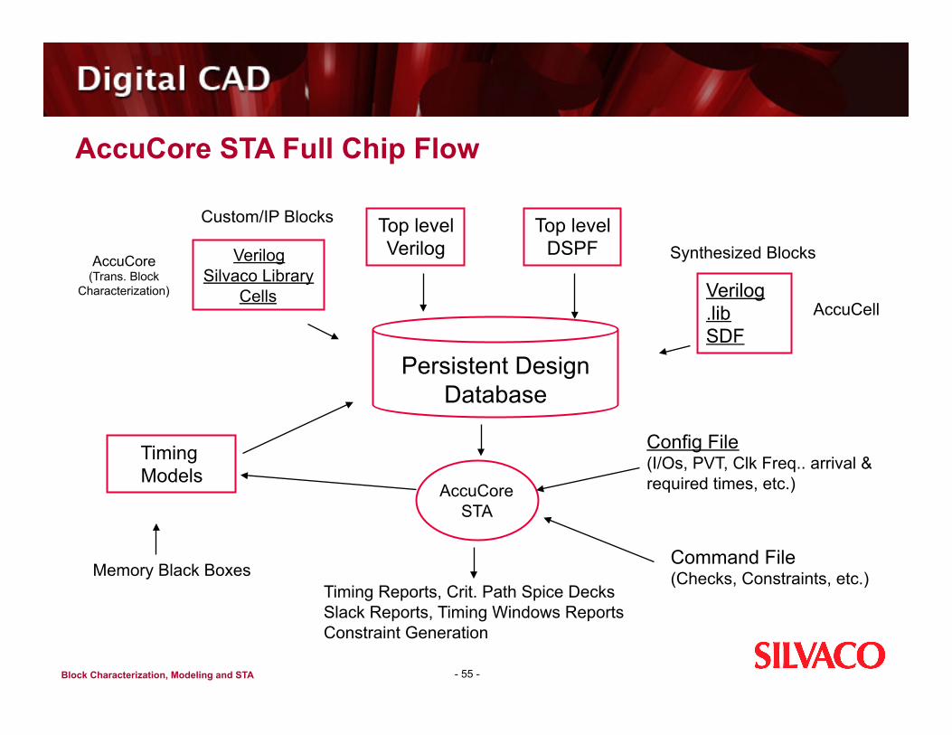
AccuCore STA Full Chip Flow
- 55 -
Custom/IP Blocks
Verilog Silvaco Library
Cells
Top level Verilog
Top level DSPF Synthesized Blocks
Verilog .lib SDF
AccuCore (Trans. Block
Characterization)
Persistent Design Database
Timing Models
AccuCore STA
Config File (I/Os, PVT, Clk Freq.. arrival & required times, etc.)
Command File (Checks, Constraints, etc.) Memory Black Boxes
Timing Reports, Crit. Path Spice Decks Slack Reports, Timing Windows Reports Constraint Generation
AccuCell
Block Characterization, Modeling and STA
AccuCore STA – Fast Paths and Looping
Fast Paths tracing algorithms Finds longest and shortest paths through the design Traces critical and subcritical paths separately
Slack Based Pruning Finds latch to latch paths Unlimited level of transparency Ability to filter similar paths
Advanced Looping algorithm Sequential loop analysis uses Depth First Search (DFS) if necessary Finds latch loop violations, clipping, latch depth violation Detection of combinational loops and scc’s
- 56 -
Block Characterization, Modeling and STA
AccuCore STA – Timing and Rules
Timing Verification: Verifies timing of flip-flop, complex latches, domino logic, dynamic
elements, muxes, and tristate elements Automatic gated-clock analysis, based on identified function Provides capability to perform data to data timing checks for arbitrary
nets in the design Rule based cycle path control
Default set of rules for synchronization Default set of rules for setup and hold checks Multi-cycle path specification
Default set of timing rules for domino circuits can be customized
- 57 -
Block Characterization, Modeling and STA
AccuCore STA – Options and Clock Specs
Has multiple options which help direct and limit paths search to area of interest Uses output function to propagate constants Elaborate path/arc/net blocking capabilities Advance capabilities to handle clock propagation
Clock specification and propagation Concept of reference clocks, primary clocks, derived clocks Rule based clock propagation uses information about cells and arcs
from the timing library User can stop or force clock propagation Different ways to handle clock choppers and clock generators
- 58 -

Block Characterization, Modeling and STA
AccuCore STA – Clocks and Busses
Automatic gated clock recognition Default timing checks Customized timing checks
Bus Contention Analysis Tristate capabilities
Data to data timing checks for arbitrary nets Handles designs with clocks of different frequency Any timing check can be customized, option to make sequential
element non-transparent Removal of common skew
- 59 -
Block Characterization, Modeling and STA
AccuCore STA - Reporting
Reporting Report of longest and shortest paths Timing check reports include clock path and data paths Separated internal and interface reporting Path based net slack report Global net based slack report provides worst arrival and required time
on the net Timing windows report with worst falling and rising arrival time on the
net Bus contention report
Reports are customizable
- 60 -
Block Characterization, Modeling and STA
AccuCore STA – Delay Calc
Delay calculation Support scalar; 1-dimensional and 2-dimensional tables of slope and
delay values as function of input slope and output load Support scalar; one-dimensional and 2-dimensional tables of setup and
hold values as function of clock slope and data slope Support conditional delays. Store multiple max and min delay records
with different vectors in Silvaco library Mode analysis
DSPF based delay calculation RC net is modeled as pairs of driver- receiver models Ceff based delay calculation algorithm
SDF interconnect delay annotation Wire delay model
- 61 -
Block Characterization, Modeling and STA
AccuCore STA – SPICE Decks and Debugging
Spice deck generation Generates spice deck of critical paths Generated spice deck of clock tree
Debugging capabilities Provides complete information about clock propagation and clock
waveforms, stopped clocks, converge clocks, etc. Provides miscellaneous netlist, library and analysis verification
commands Reports clock domain intersection, non tristate bus drivers, unknown
clock gating, latch groups. Accept consecutive configuration files within one run
- 62 -
Block Characterization, Modeling and STA
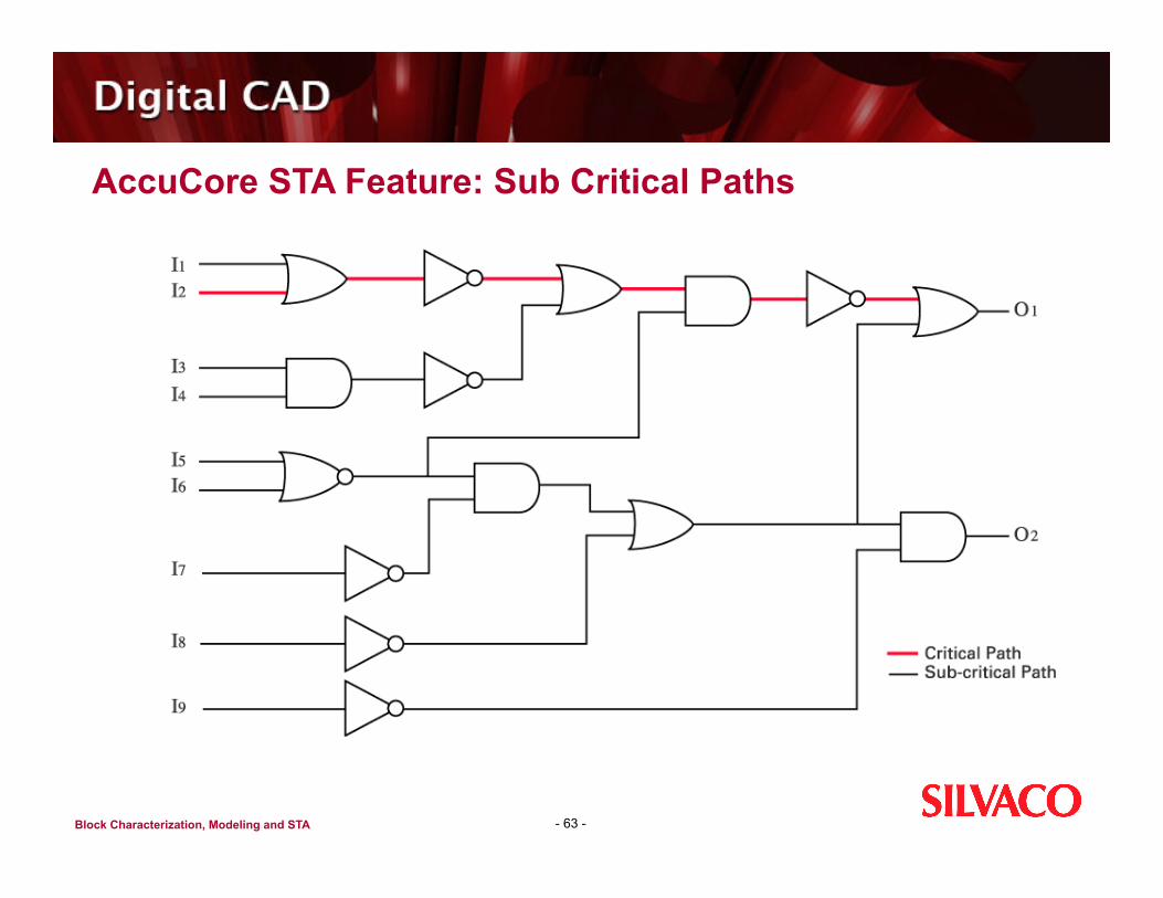
AccuCore STA Feature: Sub Critical Paths
- 63 -

LAB 4
STA Basics
Block Characterization, Modeling and STA
Lab 4 – Objectives
Use AccuCore to characterize a multiplier circuit Use AccuCore STA to perform Static Timing Analysis on a block
- 65 -
Block Characterization, Modeling and STA
STA Timing Modeling
Modeling capabilities Generates black box timing view of the design Generates compressed model timing view of the design hiding details
of combinatorial paths Propagates slope tables during compress model generation Generates interface models with the detailed view of interface logic Model verification option
- 66 -
Block Characterization, Modeling and STA
STA Clock Skew Analysis
Global Skew Global Skew can be specified as min/max clock waveforms Ability to adjust margin for gates controlled by primary or reference
clock Local Skew Ability to specify local skew relationship between clock nets. The
local skews property “getting propagated” starting from clock nets with skew along clock tree
During min analysis STA will propagate all paths to the timing checkpoints and account for the worst skew
During max analysis all path will be calculated using local skew at latch transparency points and the local skew will apply at setup check points
- 67 -

Block Characterization, Modeling and STA
STA Constraint Generation
Constraint generation for ASIC blocks and Custom blocks Min/max rise/fall arrival times and slopes at block inputs Min/max rise/fall required times and cload/ceff at block outputs Multiple input/output constraints for different reference clocks Constraints are generated to block pins for ASIC blocks Custom block constraints are generated to gate (transistor) pins For custom blocks transistor pin information is preserved for top level
DSPF back annotation Analysis support multiple input/output timing specs “per pin”
Slack allocation algorithms User controlled allocation to driver and receiver 100% allocation to driver and receiver)
- 68 -
Block Characterization, Modeling and STA
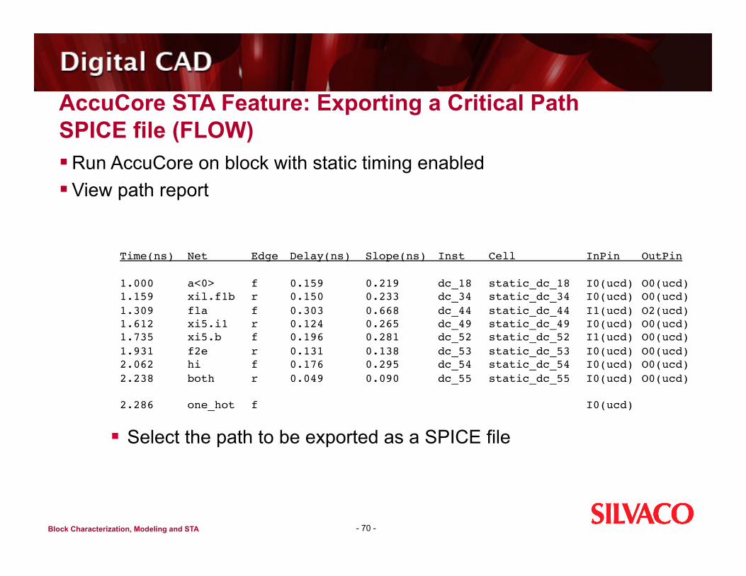
AccuCore STA Feature: Exporting a Critical Path Spice File
- 69 -
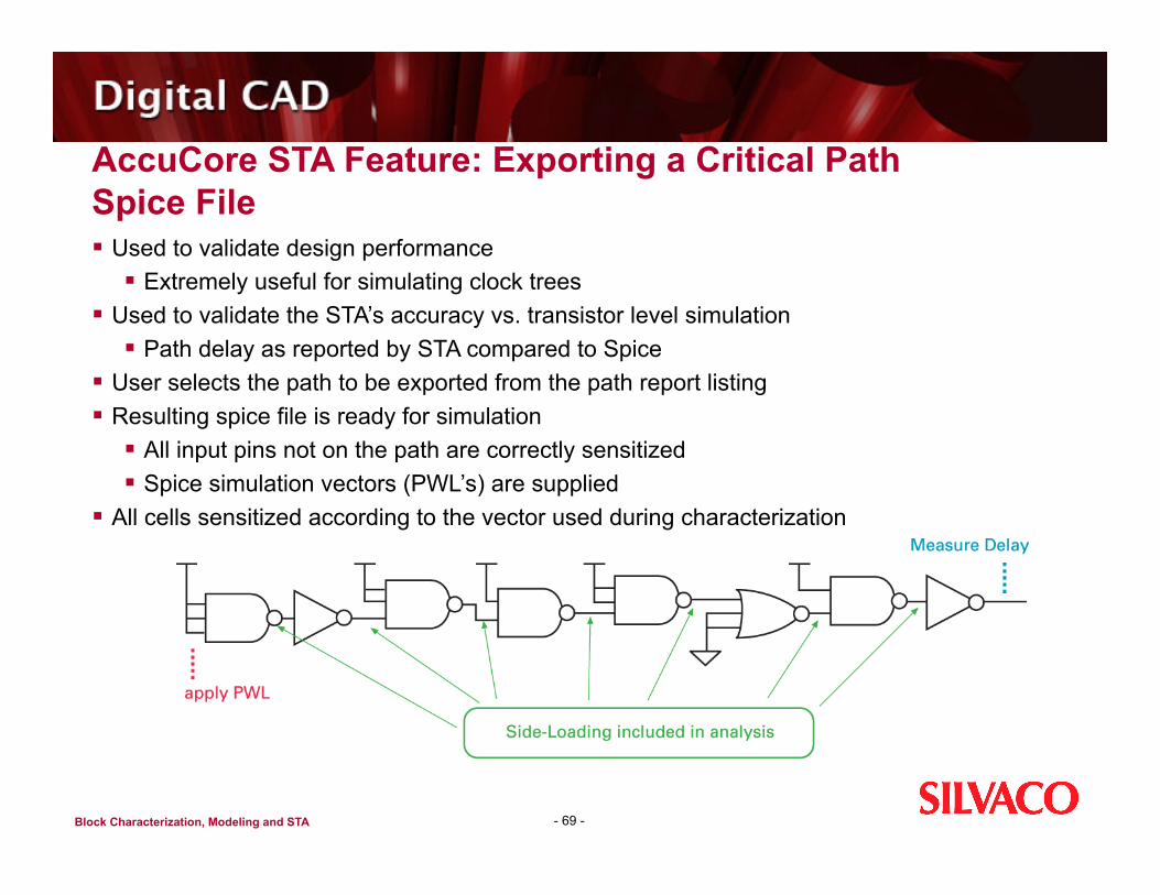
Used to validate design performance Extremely useful for simulating clock trees
Used to validate the STA’s accuracy vs. transistor level simulation Path delay as reported by STA compared to Spice
User selects the path to be exported from the path report listing Resulting spice file is ready for simulation
All input pins not on the path are correctly sensitized Spice simulation vectors (PWL’s) are supplied
All cells sensitized according to the vector used during characterization
Block Characterization, Modeling and STA
AccuCore STA Feature: Exporting a Critical Path SPICE file (FLOW) Run AccuCore on block with static timing enabled View path report
- 70 -
Select the path to be exported as a SPICE file
Time(ns) Net Edge Delay(ns) Slope(ns) Inst Cell InPin OutPin
1.000 a<0> f 0.159 0.219 dc_18 static_dc_18 I0(ucd) O0(ucd) 1.159 xil.f1b r 0.150 0.233 dc_34 static_dc_34 I0(ucd) O0(ucd) 1.309 fla f 0.303 0.668 dc_44 static_dc_44 I1(ucd) O2(ucd) 1.612 xi5.i1 r 0.124 0.265 dc_49 static_dc_49 I0(ucd) O0(ucd) 1.735 xi5.b f 0.196 0.281 dc_52 static_dc_52 I1(ucd) O0(ucd) 1.931 f2e r 0.131 0.138 dc_53 static_dc_53 I0(ucd) O0(ucd) 2.062 hi f 0.176 0.295 dc_54 static_dc_54 I0(ucd) O0(ucd) 2.238 both r 0.049 0.090 dc_55 static_dc_55 I0(ucd) O0(ucd)
2.286 one_hot f I0(ucd)
Block Characterization, Modeling and STA
AccuCore STA Feature: Exporting a Critical Path SPICE file (FLOW) (cont’d) Run AccuCore on block with static timing enabled View path report Select the path to be exported as a spice file
- 71 -
Block Characterization, Modeling and STA
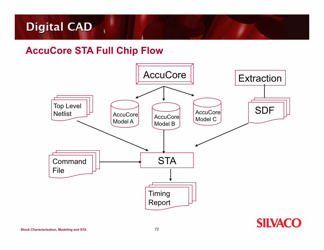
AccuCore STA Full Chip Flow
72
AccuCore
AccuCore Model C AccuCore
Model B AccuCore Model A
Top Level Netlist
Extraction
SDF
STA
Timing Report
Command File
Block Characterization, Modeling and STA
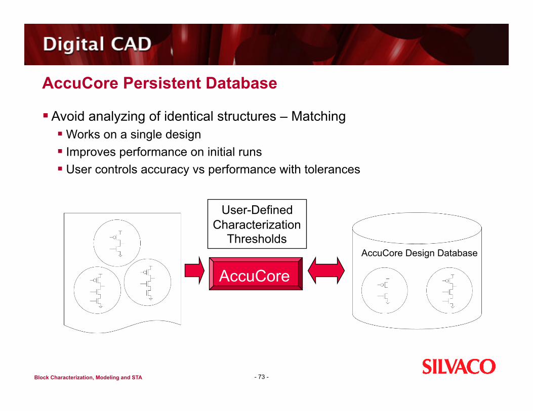
AccuCore Persistent Database
Avoid analyzing of identical structures – Matching Works on a single design Improves performance on initial runs User controls accuracy vs performance with tolerances
- 73 -
User-Defined Characterization
Thresholds AccuCore Design Database
AccuCore
Block Characterization, Modeling and STA
Summary
- 74 -
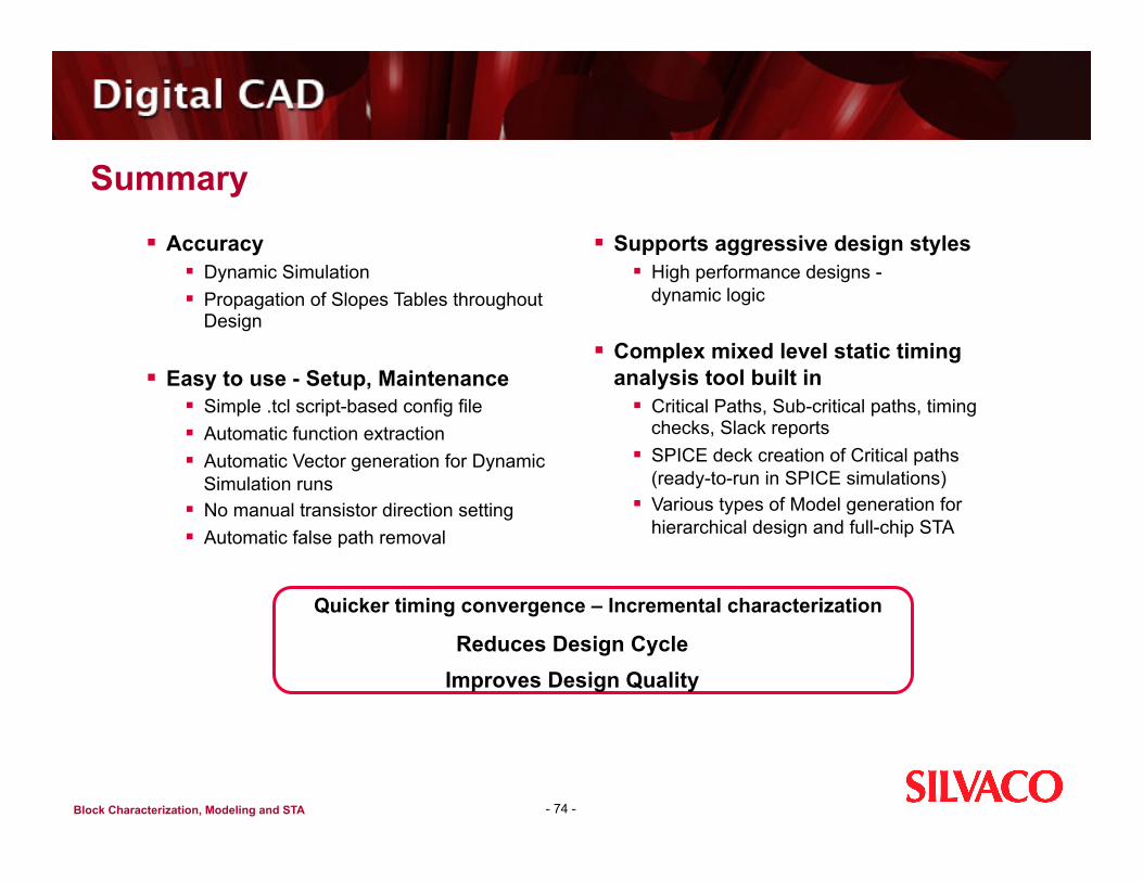
Quicker timing convergence – Incremental characterization
Reduces Design Cycle Improves Design Quality
Accuracy Dynamic Simulation Propagation of Slopes Tables throughout
Design
Easy to use - Setup, Maintenance Simple .tcl script-based config file Automatic function extraction Automatic Vector generation for Dynamic
Simulation runs No manual transistor direction setting Automatic false path removal
Supports aggressive design styles High performance designs -
dynamic logic
Complex mixed level static timing analysis tool built in Critical Paths, Sub-critical paths, timing
checks, Slack reports SPICE deck creation of Critical paths
(ready-to-run in SPICE simulations) Various types of Model generation for
hierarchical design and full-chip STA
Recommended