GEORGIA DOT RESEARCH PROJECT 10-20 FINAL REPORT
AIRPORT COSTS AND PRODUCTION TECHNOLOGY:
A TRANSLOG COST FUNCTION ANALYSIS WITH IMPLICATIONS FOR ECONOMIC DEVELOPMENT
OFFICE OF MATERIALS AND RESEARCH RESEARCH AND DEVELOPMENT BRANCH
ii
1.Report No.: FHWA-GA-11-1020
2. Government Accession No.:
3. Recipient's Catalog No.:
4. Title and Subtitle: Airport Costs and Production Technology: A Translog Cost Function Analysis with Implications for Economic Development
5. Report Date: December 2011
6. Performing Organization Code:
7. Author(s): Dr. Patrick McCarthy
8. Performing Organ. Report No.: 10-20
9. Performing Organization Name and Address: Georgia Institute of Technology School of Economics 221 Bobby Dodd Way, M/C 0615 Atlanta, GA 30332
10. Work Unit No.:
11. Contract or Grant No.: 0009929
12. Sponsoring Agency Name and Address: Georgia Department of Transportation Office of Materials & Research 15 Kennedy Drive Forest Park, GA 30297-2534
13. Type of Report and Period Covered: Final; August 2010 – July 2011
14. Sponsoring Agency Code:
15. Supplementary Notes: Prepared in cooperation with the U.S. Department of Transportation, Federal Highway Administration. 16. Abstract: Based upon 50 large and medium hub airports over a 13 year period, this research estimates one and two output translog models of airport short run operating costs. Output is passengers transported on non-stop segments and pounds of cargo shipped. The number of runways is a quasi-fixed factor of production. Statistical tests reject the null hypothesis that airport production technology is homothetic and homogeneous, exhibits constant returns to scale, or reflects a Cobb-Douglas production technology. From the analysis, airports operate under increasing returns to runway utilization and increasing ray economies of scale for the two-output model. Airport operating costs were 2% higher after the September 1, 2001 terrorist attacks. The input demand for general airport operations is price elastic, and Morishima substitution elasticities indicate that Personnel, Repair-Maintenance-Contractual services, and General Airport Operations are substitutes in production. For the one output passenger model, an exploratory analysis identifies a relationship between the average cost of airport operations and indicators of economic development. All else constant, a decrease in an airport’s real average operating costs is associated with increasing metropolitan employment, the number of establishments, and real gross metropolitan and state products.
17. Key Words: airport capacity, airport infrastructure, airport costs, economic development, panel data, runway, translog cost function, flexible form models
18. Distribution Statement: N/A
19. Security Classification: Unclassified
20. Security Classification (of this page): Unclassified
21. Number of Pages: 43
22. Price: N/A

AIRPORT COSTS AND PRODUCTION TECHNOLOGY:
A TRANSLOG COST FUNCTION ANALYSIS WITH IMPLICATIONS FOR ECONOMIC DEVELOPMENT
Patrick McCarthy School of Economics
Georgia Institute of Technology
FINAL REPORT
Submitted to
Georgia Department of Transportation Georgia Transportation Institute/University Transportation Center
December 2011
The contents of this report reflect the views of the authors who are responsible for the facts and the accuracy of the data presented herein. The contents do not necessarily reflect the official views or policies of the Georgia Department of Transportation or of the Federal Highway Administration. This report does not constitute a standard, specification, or regulation.

TABLE OF CONTENTS
List of Tables …………………………………………………………………………………...ii
Executive Summary …………………………………………………………………………….iii
I. Introduction …………………………………………………………..…………………..1
II. Review of Literature ………………………….…….……………………..……………...2
III. Empirical Methodology …………………………..………………..……………………..5
III.1 Translog Cost Function for Metropolitan Statistical Area (MSA) Airports……..……...5
III.2 Translog Cost Function – Estimation Considerations ……………………………….…7
IV. Data Sources and Descriptive Analysis ……. …….……………………………….…….9
V. Estimation Results ………………………………..………………………………..…....12
V.1 Preliminary Estimation …………………………………………………………………12
V.2 Final Estimation Results ……………………………………………………………..…14
V.2.1 Economies of Airport Runway Utilization ……………………….………………14
V.2.2 September 11, 2011 Terrorist Attacks ……………..……………………………..16
V.2.3 Demand and Substitution Elasticities …………………………………………….17
V.2.4 Average and Marginal Production Costs …………………………………………19
V.2.5 Atlanta’s Hartsfield-Jackson International Airport ………………..…………..…21
VI. Discussion and Potential Implications for Economic Development ……………………23
VII. Extensions ……………………………………………………………..…………….…..25
VII.1 Airport Operating Characteristics …………………………………………………….25
VII.2 Two Output Model with Non-Aero Operating Characteristics …………………....…30
VIII. Concluding Comments.……………………………………………………………….…36
IX. Acknowledgement.……………………………………………………………………...38
X. References….……………………………………………………………………………38
ii
LIST OF TABLES
Table 1 MSA Airport Output and Nominal Operating Costs, 1996-2008.……………………...11 Table 2 Input Price Indices (1996=100): Panel of 50 Airports, 1996-2008...……………….….12 . Table 3 Base Translog Model – Wald Specification Tests..…………………………………….13 Table 4 Translog Airport Cost Estimation Results, 1996-2008: Output – Passengers, No
Non-Aero Operating Characteristics.………………..…………………………………..15 Table 5 (a) Input Demand Elasticities.……..…………………………………………………....17 Table 5 (b) Morishima Elasticities of Substitution………………………………..…………….17 Table 6 Average and Marginal Cost: $ Million per Million Passengers..…………….…………19 Table 7 Average and Marginal Cost for Large and Medium Hub Airports, 1996-2008………...20 Table 8 Cost and Production Characteristics for Hartsfield-Jackson Atlanta International Airport.……………………………………………………………………..……….…..22 Table 9 Average Airport Operating Costs and Indicators of Economic Development, 1990-2008 …………………………………………………………………………….....24 Table 10 Average Airport Operating Costs and Gross Metropolitan Product, 2001-2008 ……..25 Table 11 Translog Airport Cost Estimation Results, 1996-2008: Output – Passengers, With Non-Aero Operating Characteristics …….……………………………….….......27 Table 12(a) Input Demand Elasticities with Non-Aero Operating Characteristics..…………….29 Table 12(b) Morishima Elasticities of Substitution with Non-Aero Operating Characteristics....29 Table 13 Average and Marginal Cost with Non-Aero Operating Characteristics: $ Million per
Million Passengers ….………………………………………………..………………….29 Table 14 Freight Shipped, 1996-2008..……..……..………………………….…………………30 Table 15 Translog Airport Cost Estimation Results, 1996-2008: Output – Passengers, Freight;
With Non-Aero Operating Characteristics..……………………………..………………33 Table 16 Two Output Model: Economies of Scale and Scope Measures …….………………...34 Table 17(a) Two Output Model: Input Demand Elasticities……………….….…………….…..34 Table 17(b) Two Output Model: Morishima Elasticities of Substitution…………….…………34 Table 18 Average and Marginal Cost: $ Million per Million Passengers, With Non-Aero Operating Characteristics.………………………………………………………………34
iii
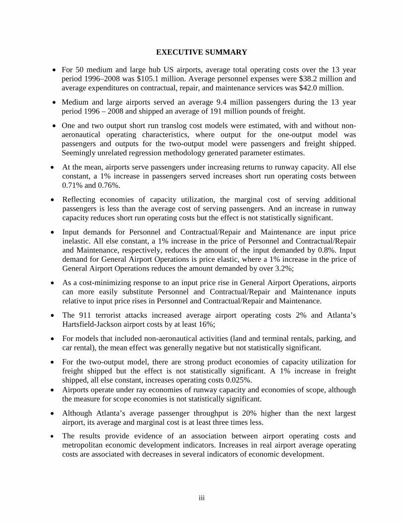
EXECUTIVE SUMMARY
• For 50 medium and large hub US airports, average total operating costs over the 13 year period 1996–2008 was $105.1 million. Average personnel expenses were $38.2 million and average expenditures on contractual, repair, and maintenance services was $42.0 million.
• Medium and large airports served an average 9.4 million passengers during the 13 year period 1996 – 2008 and shipped an average of 191 million pounds of freight.
• One and two output short run translog cost models were estimated, with and without non-aeronautical operating characteristics, where output for the one-output model was passengers and outputs for the two-output model were passengers and freight shipped. Seemingly unrelated regression methodology generated parameter estimates.
• At the mean, airports serve passengers under increasing returns to runway capacity. All else constant, a 1% increase in passengers served increases short run operating costs between 0.71% and 0.76%.
• Reflecting economies of capacity utilization, the marginal cost of serving additional passengers is less than the average cost of serving passengers. And an increase in runway capacity reduces short run operating costs but the effect is not statistically significant.
• Input demands for Personnel and Contractual/Repair and Maintenance are input price inelastic. All else constant, a 1% increase in the price of Personnel and Contractual/Repair and Maintenance, respectively, reduces the amount of the input demanded by 0.8%. Input demand for General Airport Operations is price elastic, where a 1% increase in the price of General Airport Operations reduces the amount demanded by over 3.2%;
• As a cost-minimizing response to an input price rise in General Airport Operations, airports can more easily substitute Personnel and Contractual/Repair and Maintenance inputs relative to input price rises in Personnel and Contractual/Repair and Maintenance.
• The 911 terrorist attacks increased average airport operating costs 2% and Atlanta’s Hartsfield-Jackson airport costs by at least 16%;
• For models that included non-aeronautical activities (land and terminal rentals, parking, and car rental), the mean effect was generally negative but not statistically significant.
• For the two-output model, there are strong product economies of capacity utilization for freight shipped but the effect is not statistically significant. A 1% increase in freight shipped, all else constant, increases operating costs 0.025%.
• Airports operate under ray economies of runway capacity and economies of scope, although the measure for scope economies is not statistically significant.
• Although Atlanta’s average passenger throughput is 20% higher than the next largest airport, its average and marginal cost is at least three times less.
• The results provide evidence of an association between airport operating costs and metropolitan economic development indicators. Increases in real airport average operating costs are associated with decreases in several indicators of economic development.
1
I. Introduction
Commercial air travel and air freight have grown substantially over the past fifteen years.
Between January 1995 and November 2009, passenger enplanements have increased 31.6% from
41.7 million to 54.9 million. At 572 million miles in November 2009, revenue freight miles have
increased 33.6% during the same period, a bit less than the 40.9% increase in revenue passenger
miles between January 1996 and November 2009.1 During this same period, the total number of
commercial airport runways constructed to support the traffic increased 3.3%. At airports with
significant activity where the infrastructure needs are the greatest, the number of runways
increased 14.8%.2 Without the necessary infrastructure to support the increasing demand for air
passenger travel and air freight, there will be continuing problems with system delays, airport
congestion, safety, and deteriorating services that airports provide.3 Airports are drivers of
economic development and there is an increasing literature on the positive effects that airports
have on metropolitan and, more broadly, regional economic development.
This study focuses on airports, their costs and productivity. Similar to any large
enterprise, airports manage a significant amount of resources in providing the necessary
infrastructure for air transport. By allocating its resources more efficiently, an airport reduces
time and out-of-pocket costs of individuals and businesses and provides an infrastructure for the
metropolitan area and region to strengthen its economic base and develop faster. This analysis
develops and estimates single and multiple output translog models for airport operating costs.
Translog models are flexible form models which allow one to test alternative hypotheses on
production technology, including homotheticity, homogeneity, returns to scale, and elasticity of
substitution.4 From the results, cost estimates are used to explore the relationship between airport
costs and metropolitan development.
1 Department of Transportation, Bureau of Transportation Statistics, http://www.bts.gov/data_and_statistics/ , 2011.
2 The Federal Aviation Administration identifies these as Operational Evolutionary Partnership (OEP) airports. The OEP 35 airports are commercial U.S. airports with significant activity. These airports serve major metropolitan areas and are hubs for airline operations. More than 70 % of passengers move through these airports. 3 Many factors enter the decision to increase runway capacity, including environmental concerns, whether there is sufficient space for a new runway, new technologies which help airports increase flows with existing capacity, and expected future demands. 4 Among the properties of homothetic functions, optimal input shares are independent of the level of output, the expansion path is linear, and the marginal rate of technical substitution is independent of the level of output. A production function is homogeneous when the scalar multiplication of all inputs increases output in some proportion to the scalar increase. A production function that is homogeneous of degree 1 exhibits constant returns to scale. Well behaved functions are positive, finite, twice continuously differentiable, strictly monotone and quasi-concave. By
2
II. Review of Literature
During the past two decades, there have been numerous studies on cost and production in
the transportation and public capital literatures using flexible form models, including Caves,
Christensen, and Swanson (1981), Deno (1988), Duffy-Deno and Eberts (1991), Keeler and Ying
(1988), Lynde and Richmond (1992), Morrison and Schwartz (1996). Among the more widely
used approaches are the translog and generalized Leontief cost functions.
Caves, Christensen, and Swanson (1981) develop and estimate multiproduct variable or
short run cost functions on a pooled cross section of railroad firms in the United States for 1955,
1963, and 1974. Using ton-miles of freight, average length of freight haul, passenger-miles and
average length of passenger trips as output indexes and labor, fuel, and equipment as input
indexes, the study estimates average annual rates of productivity growth at 2 % per year for the
sample period. The estimated elasticities of total cost with respect to the four outputs are
consistent with the hypothesis that the United States railroad systems operate with scale
economies.
Keeler and Ying (1988) analyze the effects of Federal-Aid highway infrastructure
investments on costs and productivity of U.S. firms in the motor freight transport industry.5
Based on a translog cost specification of regional trucking firms, the study finds that the rapid
growth of highway infrastructure that occurred between 1950 and 1973 produced a strong and
positive effect on productivity growth in trucking. Furthermore, the results support the position
that the benefits of these investments, narrowly defined as benefits to the trucking industry, fall
between one-third and one-half of the cost of the Federal Aid highway system over this period.
Using a translog specification, Deno (1988) analyzed the impact of public capital on
manufacturing firms’ variable input demands and output supplies.6 The study found that public
capital was an important factor in manufacturing input demand and output supplies. And in terms
of differential effects, Deno found that water public capital had the largest effect on growing
regions whereas highway capital had a larger effect on declining regions.
Duffy-Deno and Eberts (1991) estimates the effect of public capital stock on regional per
capita personal income using a two-stage-least-squares regression model. For a sample of
the principle of duality, well-behaved cost functions embody all of the economically relevant attributes of the underlying production technology (Varian, 2nd Edition, 1984). 5 Keeler and Ying, 1988, p. 69. 6 Rather than estimating a cost function, Deno (1988) estimated a translog profit function. Deno’s measure of public capital included roads and highways, sewers and sewage disposal and water and water treatment plants.
3
metropolitan areas, the study measures the quantity and quality of public capital stock using the
perpetual inventory technique. The authors find that public capital has a positive and significant
impact on per capita income, suggesting that investments in public capital enhances economic
development and, conversely, allowing public capital to deteriorate hinders metropolitan
development.
Lynde and Richmond (1992) use a translog cost function approach using annual
observations for the U.S. nonfinancial corporate sector from 1958 to 1989 to estimate the impact
of public capital (state and local and federal nonmilitary public capital) on the costs of
production in the private sector. The authors find support for the productivity of public capital
and find that public and private capital are complements rather than substitutes in production.
Morrison and Schwartz (1996) use a cost function framework to analyze the role of state
infrastructure, defined as publicly owned highway, water, or sewer material, on productivity
using a panel of the contiguous 48 states from 1970-1987. The measure of productivity growth
decomposes the traditional productivity growth "measure of our ignorance" into the impacts of
technical change, scale economies, fixity of private capital, and the availability of public
infrastructure capital.7 The authors estimate shadow values that reflect the potential cost savings
from a decline in variable inputs required to produce a given amount of output when
infrastructure investment occurs.8 The positive shadow value for public capital supports the
inference that the return to infrastructure investment is economically significant and suggests that
slowdowns in public infrastructure investment reduce productivity growth.
Brox and Fader (2005) examine the relationship between Canadian public infrastructure
and private output using a constant elasticity of substitution translog cost model. The study finds
that Canadian infrastructure, as measured by the accumulated stock of public infrastructure, is a
substitute for private capital and that during the period of the study, 1961-1997, economies of
scale characterized manufacturing costs.9
Although many of the above flexible form studies focus upon the development effects of
transportation and other forms of public capital, none of these analyze the effect of airport
infrastructure upon economic development. However, there are a number of studies that have
7 Morrison and Schwartz, 1996, p. 1100. 8 Morrison and Schwartz, 1996, p. 1095-1096. 9 Brox and Fader, 2005, p. 1254.

4
analyzed the impact that airport output has upon metropolitan development, using enplaned
passengers as a measure for airport output.
Goetz (1992) tests the hypothesis that the growth of air passenger travel affects the urban
system and its development. Based upon Census population and employment data for 1950,
1960, 1970, 1980, and 1987 for the 50 largest air passenger cities for each of these years, Goetz
finds that increases in per capita passenger flows are positively correlated with past and future
growth, consistent with the importance that air travel has for economic development. Hakfoort et
al. (2001) and Brueckner (2003) explore the impact that airports have upon metropolitan
employment. Using an input-output framework to trace the effects of an expansion of
Amsterdam’s Schiphol Airport on the Greater Amsterdam region from 1987 – 1998, Hakfoort et
al. find that a one job increase at Schiphol produces 1 job from indirect and induced effects,
producing 42,000 jobs in 1998. Exploring linkages between employment and air traffic in the
Chicago metropolitan area, Brueckner (2003) finds that a 1% increase in passenger enplanements
increases employment in service-related industries 0.1%. An important implication from
Brueckner’s analysis is that an airport expansion at Chicago’s O’Hare Airport would have strong
economic development effects, generating 185,000 service-related jobs.
Rather than looking only at enplanements, Green (2007) uses various measures of airport
passenger and cargo activity to analyze the effects of airports on population and employment
metropolitan growth between 1990 and 2000. Green finds that, after controlling a city’s taxes,
climate, industrial structure, human capital, commute time, and the impact that growth in
passenger activity has on population and employment growth (i.e. reverse causality), passenger
activity is a strong predictor of population and employment growth.
Two recent studies on airports have addressed questions of governance and airport
efficiency and network effects. Based upon a set of airports worldwide, Oum et al. (2007) uses a
stochastic frontier approach to analyze airport efficiency and implications this may have for
airport governance. Generally, the authors find that privatizing airports will enhance airport
efficiency, and by inference, economic development. An exception to this is mixed ownership
structures, with government majority, which the authors find to be less efficient than 100%
publicly owned airports. Oum et al. also found that there would be efficiency gains if the
management of an airport in a metropolitan area with multiple airports is privatized,
corporatized, or an independent airport authority in place of government management.
5
Cohen and Paul (2003) explore the extent to which changes in airport infrastructure have
network-associated development effects. Based upon a generalized Leontif empirical model and
using state level data for the manufacturing sector in the 48 continental United States from 1982
– 1996, the authors not only find that a state’s airport infrastructure investment lowers
manufacturing costs in an airport’s own state but also that other states’ airport infrastructures
lower manufacturing a state’s manufacturing costs.10 The authors attribute these benefits to
increases in air traffic and system reliability.
III. Empirical Methodology
Minimizing an airport’s operating costs subject to an output constraint generates an
airport cost function that provides insights on technical aspects of an airport’s production
function. In particular, a general specification for an airport’s variable or operating costs is:
Cit = C(qit; pitj ; kit, τ)
where, for airport i at time t, Cit is total operating costs, qit is an airport’s operational output, pitk
is the price of variable input j, kit is the level of fixed capital, and τ is the state of technology.
Inputs include such factors as labor, outsourced services, repairs and maintenance, and airport
capital. Depending upon specification for the empirical model, estimating this cost function can
provide information on scale economies, factor demands and their prices, and elasticities of
substitution. In addition, marginal and average costs of production are straightforward outputs
from the analysis.
III.1 Translog Cost Function for Metropolitan Statistical Area (MSA) Airports
A commonly employed flexible form cost function is the translog function whose general
form for total operating costs is
(2) ∑=
−+−+−+−+=J
jijitjjiitiitkiitqit ppkkqqVC
10 )ln(ln)ln(ln)ln(ln)ln(lnln βττββββ τ
10 The measure of other states’ airport infrastructure is a weighted average that accounts for passenger trips between the two states and the relative size of state level economic activity.

6
∑=
−−+−+−+J
jimitmijitjjmiitkkiitqq ppppkkqq
1
22 )ln)(lnln(ln2
1)ln(ln
2
1)ln(ln
2
1 βββ
)ln)(lnln(ln)ln(ln)ln(ln)ln(ln)ln(ln11
iitiqkiit
J
jijitjjkiit
J
jijitjjq kkqqkkppqqpp −−+−−+−−+ ∑∑
==
βββ
VCit is the airport’s total operating cost, qit is output, pitj (i = 1, … , J) is the price of the j th input,
kit is the level of quasi-fixed capital, and τit is the state of technology for airport i at time t,. τit
captures shifts in the cost function due to technological progress in the industry. The bar
indicates a variable’s mean value.
A well-behaved cost function with a quasi-fixed factor must satisfy several conditions:
(a) linear homogeneity in factor prices and (b) symmetry in factor prices, (c) monotonicity and
(d) concavity.11 The following restrictions ensure that the cost function satisfies these properties:
(3) ,1J
1jj∑ =β
=
0J
1j
J
1mjm
J
1jjm
J
1mjm ∑ =∑ β∑ =β∑ =β
= ===
∑ =β=
J
1jjq 0; ∑ =β
=
J
1jjm 0 ; ∑ =β
=τ
J
1jj 0.
The symmetry restriction requires that βij = βji. If the cost function satisfies monotonicity and
concavity, then input shares have positive signs at all observations and the matrix of substitution
elasticities is negative semidefinite for any combination of cost shares, respectively.12
The translog cost function imposes no a priori restrictions on input substitution
possibilities or scale economies. Further, differentiating the cost function with respect to factor
prices (Shephard, 1970) yields cost share equations Si’s for each of the j variable inputs. In
particular,
(4) )ln(ln)ln(ln)ln(ln2
1
1iitikiitiqijijt
n
jijii kkqqppS −+−+−+= ∑
=
ββββ
11 Christensen, Jorgenson, and Lau (1975) and Berndt and Wood (1975). A cost function is homogeneous of degree one in prices when prices and total costs move proportionately, all else equal. A cost function that is non-decreasing in factor prices satisfies monotonicity. 12 A symmetric matrix is negative semidefinite if all characteristic roots are nonpositive (Greene, 2000, p. 47).

7
Consistent with other analyses, Morishima partial substitution elasticities Mijσ provide measures
of substitution between factor inputs and specifically measures the impact on the input ratio from
a factor price increase as:13 :
(5) j
jijjij
Mij p
)x/xln(
∂∂=η−η=σ
where pj is the price of factor j (Chambers, 1988) and ηij is the elasticity of input i with respect
to price of input j.
In the presence of quasi-fixed and other factors of production that are difficult to adjust,
Caves et al. (2002) demonstrates that for the single output case, economies of capital stock
utilization (i.e. the returns to scale given the quasi-fixed factor) are:
(6) ECUit =
it
it
it
it
Q
VC
K
VC
ln
ln
ln
ln1
∂∂
∂∂−
= .)ln(ln)ln(ln)ln(ln(
)ln(ln)ln(ln)ln(ln1
ijitj
J
jjiitqkiitqqq
ijitj
J
jjiitqkiitkkk
ppkkqq
ppqqkk
−+−+−+
−+−+−+−
∑∑ββββ
ββββ
At mean values of production, input prices, and quasi-fixed capital, ECUit is (1/βq). Finally,
through the introduction of time variables, one can explore the effects of technological change on
costs.
III.2 Translog Cost Function – Estimation Considerations
For the translog model identified in equation (2), there are two sets of restrictions. First,
and summarized in equation (3), are restrictions to ensure that the cost function is well-behaved.
These restrictions are imposed on the model before estimation. Second, as a flexible functional
form, the translog model is a specification under which simpler models are nested. In particular,
we can test for homotheticity, homogeneity, Cobb-Douglas, and constant returns to scale:
a) If βlq = βeq = then the underlying production function is homothetic, i.e. the input ratio
is a function of the input price ratio;14
13
An alternative measure for substitution effects is the Allen-Uzawa measure which is a one factor-one price measure. Morishima’s measure is a two factor-one price measure which better reflects substitutability between inputs. Chamber (1988) demonstrates that Allen-Uzawa substitutes are Morishima substitutes but two factors may be Allen-Uzawa complements but Morishima substitutes. That is, in contrast to Allen-Uzawa, Morishima’s measure is not sign symmetric.

8
b) If a) is true and βqq = 0, then the underlying production function is homothetic and
homogeneous, i.e. if there is a proportionate (e.g. doubling) increase in all variable
inputs, then output increases by some power r of the proportionate increase;15
c) If a) and b) are true and βq = 1, then we have constant returns to scale;
d) If a) and b) are true and βle = βll = βee = 0, then the underlying production function is
Cobb-Douglas with elasticities of substitution equal to 1. In addition, if βq = 1, then
the Cobb-Douglas production technology also has constant returns to scale.
Because the data include a panel of 50 airports from 1996 – 2008, we also estimate a full set of
fixed effects, αi (i = 1, …., 49), where the constant term β0 is the reference airport, Florida’s
Tampa International Airport.
In order to increase the efficiency of the parameter estimates, the cost function (equation
2) and the share equations (equation 4) are estimated jointly as a system. In particular,
(7) ∑∑==
−+−+−+−++=J
jijitjjiiiitkiitq
iiit ppkkqqVC
1
34
10 )ln(ln)ln(ln)ln(ln)ln(lnln βττβββαβ τ
∑=
−−+−+−+J
jimitmijitjjmiitkkiitqq ppppkkqq
1
22 )ln)(lnln(ln2
1)ln(ln
2
1)ln(ln
2
1 βββ
)ln)(lnln(ln)ln(ln)ln(ln)ln(ln)ln(ln11
iitiitqkiit
J
jijitjjkiit
J
jijitjjq kkqqkkppqqpp −−+−−+−−+ ∑∑
==
βββ
JjkkqqppS iitkiitqijitj
J
jjii ,...,1)ln(ln)ln(ln)ln(ln
2
1
1
=−+−+−+= ∑=
ββββ
where αi (i = 1, …, 34) is the fixed effect for MSA i, J is the number of inputs, and the bar over a
variable reflects the temporal mean over cross section i. Technological progress τi for MSA i is
assumed to move with time so that τi = year for each cross section. Also, because the shares Si (i
= 1,…, J) sum to one, one input share must be dropped in order to identify the parameters. 14 The Cobb–Douglas production function is commonly used to represent the relationship of an output to inputs. It has the following form: y = ALαKβ, where y stands for total output, L is labor and K is capital. α and β measure the relative importance of labor and capital in production. Also, for homothetic production functions, slopes of the level curves (i.e. isoquants) are equal for any given input ratio and the dual cost function is separable in output and prices (Silberberg, 2nd Edition, 1990). 15
A further implication is that that the elasticity of cost function with respect to output is constant (Christensen and Greene, 1976).
9
Parameter estimates in a system of equations are invariant to the share equation dropped when
using maximum likelihood estimation procedures (Berndt (1991)).
IV. Data Sources and Descriptive Analysis
The measure of output for this analysis is the number of non-stop segment passengers
transported and is available from the Bureau of Transportation Statistics (BTS).16 Operating and
financial data for 1996 – 2008 are available from the Federal Aviation Administration (FAA)’s
Compliance Activity Tracking System (CATS, http://cats.airports.faa.gov, 2011) which includes
operating expenses. For this study, the cost analysis includes medium and large hub airports in
2011. The analysis included data on airport operating (i.e. short run) expenses and three airport
inputs: 1) personnel and benefits (p); contracting, maintenance, and repair (m), and airport
operations (e).17
Often in cost analyses, personnel expenses divided by the number of employees provides
an estimate of the (average) cost of labor. However, CATS does not request information on the
number of employees which requires an alternative measure for airport wage costs. At the MSA
level, there do not exist income or wage indices for airport personnel. Although there is income
information on airport personnel at the national level, the data series are incomplete for the
period 1996 – 2008.18 The procedure followed here was to use annual average pay information in
the Quarterly Census of Earnings and Wages. These data are not specific to airport personnel but
are specific to MSAs.19 These data were normalized to 1996, the first year of the data series.
16
Data were available from the BTS website, (http://www.transtats.bts.gov/Fields.asp?Table_ID=293), 2011. 17 Salaries and benefits are the salaries, wages, benefit and pension outlays for personnel that the airport employs. Contracting, maintenance, and repair includes supplies and materials, repairs and maintenance, and contractual services (including costs to commercial enterprise for diverse services that include management, financial, engineering, architectural, firefighting, and related). General airport operations include utilities and communication expenses, insurance costs and claims, small miscellaneous expenses, and other not reported elsewhere. For a definition of these categories, see U.S. DOT, FAA, Advisory Circular AC No: 150/5100-19C, April 19, 2004, Guide for Airport financial Reports Filed by Airport Sponsors. Repairs and maintenance and contractual services were combined because many airports reported $0 under repairs and maintenance but large costs under contractual services, suggesting that many repairs and maintenance activities, including runways, were subcontracted to third parties. These subcontracts fall under FAA’s Technical Support Services Contract in its Capital Investment Plan. Included among general airport operations were those categories of expenses that individually were relatively small. 18 An initial strategy was to obtain wage information from the Bureau of Labor Statistics, U.S. Department of Labor, Occupational Employment Statistics (www.bls.gov/oes), categories 48-49 (Transportation and Warehousing), 488 (Support Activities for Transportation), 4881 (Support Activities for Air Transportation)' and '48811' (Airport Operations). 19
Bureau of Labor Statistics, U.S. Department of Labor, Occupational Employment Statistics (http://www.bls.gov/cew/data.htm , 2011). Data for this analysis is NAICS based annual data, aggregate level 40 (Total MSA Covered).
10
MSA price indices for contracting, maintenance, and repair are not available but there exist
related series at the national level. Because this category reflects, among other activities, major
and minor repair activities, a price index for material and supply inputs to nonresidential building
construction was used to estimate prices for this category.20 In order to capture price differences
across metropolitan areas, the national index was multiplied by a MSA regional price index and
normalized to 1996.
A similar procedure was followed to obtain a price index for general airport operations.
For the period 1996-2008, a national price index for ‘Other Airport Operations, adjusted for
MSA price differences and normalized to 1996, was used to reflect prices for general airport
operations.21
Tables 1 and 2 provide descriptive statistics for airport cost categories and price indices
used for the cost analysis. Over the entire sample, an airport annually spends, on average, $38.2
million on personnel (36.4%), $42.0 million on maintenance and repair (40.0%, including
Contractual), and $24.9 million (23.7%) on general airport operations. As expected, the variation
in average expenses across time is smaller than the variation across airports. For example,
average variation in personnel expenses over the 13 year period (1996 – 2008) is $63.2 million in
comparison with $130.1 million average variation among the 50 airports.
For the full sample, airports on average transported 9.2 million passengers transported on
non-stop segments with a 7.2 million standard deviation. When summed over years, the standard
deviation across airports is 25.9 million passengers. California’s Burbank Bob Hope Airport
served the least and Atlanta served the largest number of passengers, averaging 2.56 and 35.9
million, respectively, over the 13 year period.
Reflecting airport operating characteristics of airports, Table 1 also presents revenues that
airports receive from its land and terminal facilities, parking, and rental cars. For the full sample,
airport physical facilities generated $5.7 million (7.5%), parking revenues were $30.9 million
(40.0%), and revenues from car rentals were $14.4 million (18.6%).
20
Bureau of Labor Statistics, U.S. Department of Labor, Consumer Price Index, CPI Databases, http://www.bls.gov/cpi/data.htm (series BBLD--, Material and supply inputs to nonresidential building construction). 21
Bureau of Labor Statistics, U.S. Department of Labor, Consumer Price Index, CPI Databases, http://www.bls.gov/cpi/data.htm , 2011 (series 488119P, Other airport operations as the primary activity, which includes operating airports and supporting airport operations. Price indices for series 48811 (Support Activities for Airport Operations) and 48811 (Airport Operations) were not available for 1996-2002.

11
Table 1
MSA Airport Output and Nominal Operating Costs, 1996-2008
Variable
# of Obser-vations Mean
Standard Deviation
Contractural Services/Repairs and Maintenance ($) 650 $42,002,127 62,204,985
General Airport Operations ($) 650 24,919,411 42,778,270
Personnel compensation and benefits ($) 650 38,233,191 38,340,527
Operating Expenses, Total ($) 650 105,154,729 106,049,390
Non Aero Operating Revenue, Land and Non-Terminal Facilities ($) 650 5,775,584 11,993,192
Non Aero Operating Revenue, Parking ($) 650 30,953,354 23,296,475
Non Aero Operating Revenue, Rental Cars ($) 650 14,393,518 10,739,802
Airport, Domestic Passengers by U.S. and Foreign Air Carriers 650 9,405,722 7,253,000
Contractural Services/Repairs and Maintenance ($) 650 $42,002,127 187,801,559
General Airport Operations ($) 50 24,919,411 138,649,596
Personnel compensation and benefits ($) 50 38,233,191130,107,858
Operating Expenses, Total ($) 50 105,154,729 363,494,817
Non Aero Operating Revenue, Land and Non-Terminal Facilities ($) 50 5,775,584 33,878,724
Non Aero Operating Revenue, Parking ($) 50 30,953,35476,569,509
Non Aero Operating Revenue, Rental Cars ($) 50 14,393,518 35,248,937
Airport, Domestic Passengers by U.S. and Foreign Air Carriers 50 9,405,722 25,907,585
Contractural Services/Repairs and Maintenance ($) 13$42,002,127 120,134,081
General Airport Operations ($) 13 24,919,411 45,567,868
Personnel compensation and benefits ($) 13 38,233,19163,247,402
Operating Expenses, Total ($) 13 105,154,729 175,979,018
Non Aero Operating Revenue, Land and Non-Terminal Facilities ($) 13 5,775,584 11,993,192
Non Aero Operating Revenue, Parking ($) 13 5,775,584 5,000,110
Non Aero Operating Revenue, Rental Cars ($) 13 30,953,354 55,706,131
Airport, Domestic Passengers by U.S. and Foreign Air Carriers 13 14,393,518 21,664,453
Group
Average over
Full Sample
Airports
Average over
Average over
Years
Source: Federal Aviation Administration Compliance Activity Tracking System (CATS, http://cats.airports.faa.gov, 2011)

12
Table 2
Input Price Indices (1996 = 100) Panel of 50 Airports, 1996 – 2008
Variable
# of Observ-ations Mean
Standard Deviation
Price Index, Contractural Services/Repairs and Maintenance 650 143 31Price Index, General Airport Operations 650 129 18Price Index, Personnel compensation and benefits 650 134 31Price Index, Contractural Services/Repairs and Maintenance 50 143 17Price Index, General Airport Operations 50 129 12Price Index, Personnel compensation and benefits 50 134 16Price Index, Contractural Services/Repairs and Maintenance 13 143 224Price Index, General Airport Operations 13 129 130Price Index, Personnel compensation and benefits 13 134 228
Average overAirports
Average overYears
GroupAverage over
Full Sample
Source: Federal Aviation Administration Compliance Activity Tracking System (CATS, http://cats.airports.faa.gov, 2011)
Table 2 reports price indices for the three inputs where each index equals 100 for 1996.
Over the entire sample, personnel expenses in MSAs have on average risen 29% in comparison
with a comparable 34% average increase in non-residential building materials and a 43% average
increase in airport operations. In contrast to airport expenses, the average variance in prices was
much higher across time than across airports (e.g. 228 vs. 16 standard deviation for personnel).
V. Estimation Results
V.1 Preliminary Estimation
Initially, the translog model in equation (8) was estimated with a time trend whose
coefficient was statistically insignificant. Also included in the preliminary model was an
interaction variable, the product of output and a dummy variable that equals 1 if the airport is
located in a MSA that has more than one commercial airport and 0 otherwise. This was
significant and included in the final model.
The model was re-specified with the following changes. A September 11, 2001 variable,
t911, replaced the time trend, where t911 = 0 if year < 2000 and equal to 1 if year > 2001. In
addition, in order to explore whether the September 11, 2001 terrorist attacks had a
disproportionate effect on Hartsfield-Jackson International Airport, t911 was interacted with a
new variable, ‘ATL’, which equals 1 for Hartsfield-Jackson International Airport and 0
13
otherwise. In addition, ‘ATL’ was interacted with the quasi-fixed capital variable, number of
runways, in order to explore whether there was also a differential effect of the number of
runways on airport operating expenses for Hartsfield-Jackson International Airport.
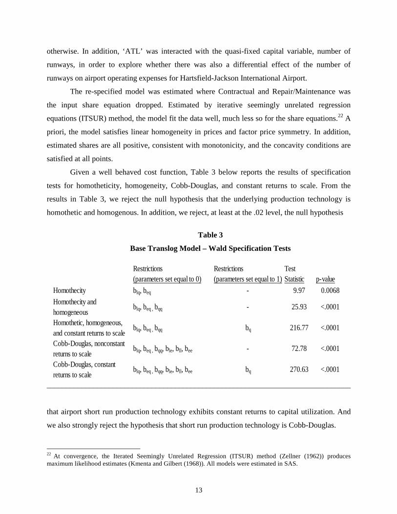
The re-specified model was estimated where Contractual and Repair/Maintenance was
the input share equation dropped. Estimated by iterative seemingly unrelated regression
equations (ITSUR) method, the model fit the data well, much less so for the share equations.22 A
priori, the model satisfies linear homogeneity in prices and factor price symmetry. In addition,
estimated shares are all positive, consistent with monotonicity, and the concavity conditions are
satisfied at all points.
Given a well behaved cost function, Table 3 below reports the results of specification
tests for homotheticity, homogeneity, Cobb-Douglas, and constant returns to scale. From the
results in Table 3, we reject the null hypothesis that the underlying production technology is
homothetic and homogenous. In addition, we reject, at least at the .02 level, the null hypothesis
Table 3
Base Translog Model – Wald Specification Tests
Restrictions Restrictions Test(parameters set equal to 0) (parameters set equal to 1)Statistic p-value
Homothecity blq, beq - 9.97 0.0068
Homothecity and homogeneous
blq, beq , bqq - 25.93 <.0001
Homothetic, homogeneous, and constant returns to scale
blq, beq , bqq bq 216.77 <.0001
Cobb-Douglas, nonconstant returns to scale
blq, beq , bqq, ble, bll, bee - 72.78 <.0001
Cobb-Douglas, constant returns to scale
blq, beq , bqq, ble, bll, bee bq 270.63 <.0001
______________________________________________________________________________
that airport short run production technology exhibits constant returns to capital utilization. And
we also strongly reject the hypothesis that short run production technology is Cobb-Douglas.
22 At convergence, the Iterated Seemingly Unrelated Regression (ITSUR) method (Zellner (1962)) produces maximum likelihood estimates (Kmenta and Gilbert (1968)). All models were estimated in SAS.
14
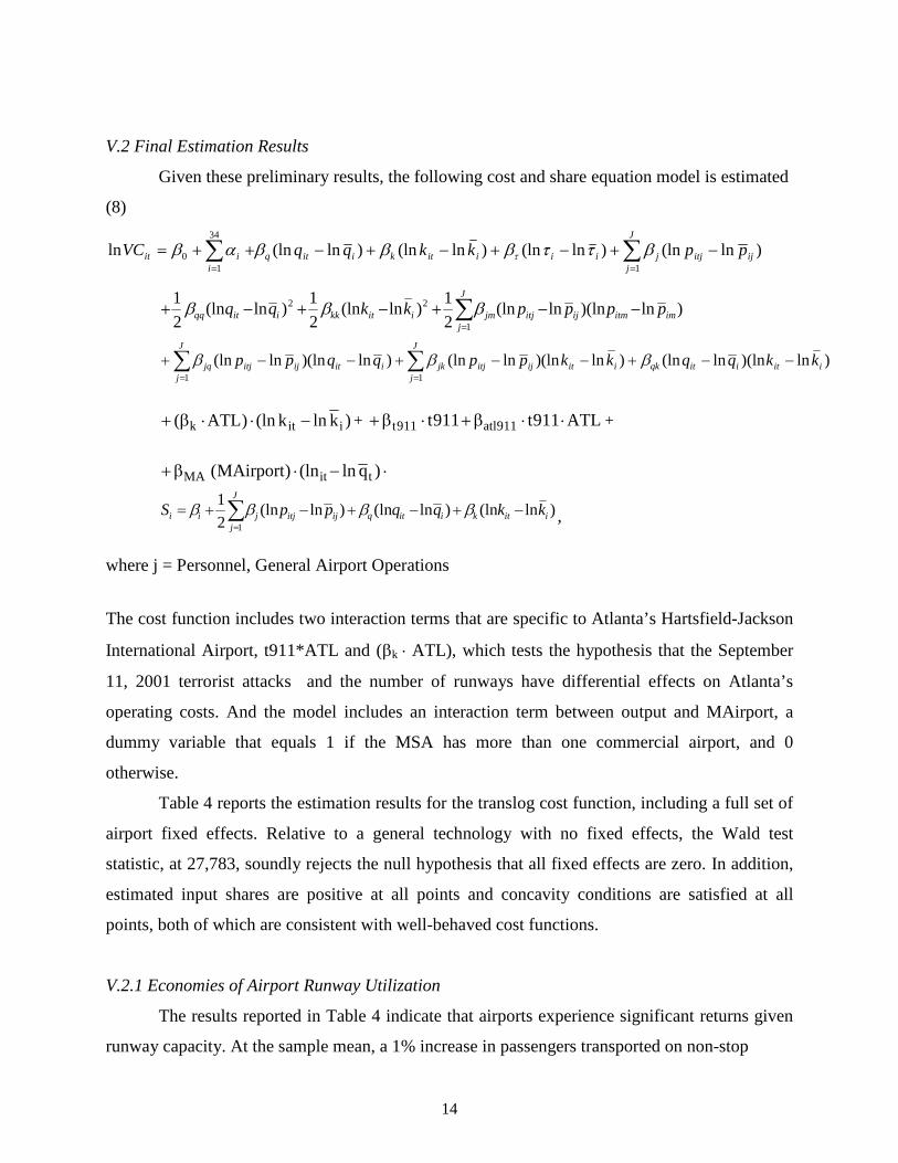
V.2 Final Estimation Results
Given these preliminary results, the following cost and share equation model is estimated
(8)
∑∑==
−+−+−+−++=J
jijitjjiiiitkiitq
iiit ppkkqqVC
1
34
10 )ln(ln)ln(ln)ln(ln)ln(lnln βττβββαβ τ
∑=
−−+−+−+J
jimitmijitjjmiitkkiitqq ppppkkqq
1
22 )ln)(lnln(ln2
1)ln(ln
2
1)ln(ln
2
1 βββ
)ln)(lnln(ln)ln(ln)ln(ln)ln(ln)ln(ln11
iitiitqkiit
J
jijitjjkiit
J
jijitjjq kkqqkkppqqpp −−+−−+−−+ ∑∑
==
βββ
)klnk(ln)ATL( iitk −⋅⋅β+ + ATL911t911t 911atl911t ⋅⋅β+⋅β+ +
⋅−⋅β+ )qln(ln)MAirport( titMA
)ln(ln)ln(ln)ln(ln2
1
1iitkiitqijitj
J
jjii kkqqppS −+−+−+= ∑
=
ββββ ,
where j = Personnel, General Airport Operations
The cost function includes two interaction terms that are specific to Atlanta’s Hartsfield-Jackson
International Airport, t911*ATL and (βk ⋅ ATL), which tests the hypothesis that the September
11, 2001 terrorist attacks and the number of runways have differential effects on Atlanta’s
operating costs. And the model includes an interaction term between output and MAirport, a
dummy variable that equals 1 if the MSA has more than one commercial airport, and 0
otherwise.
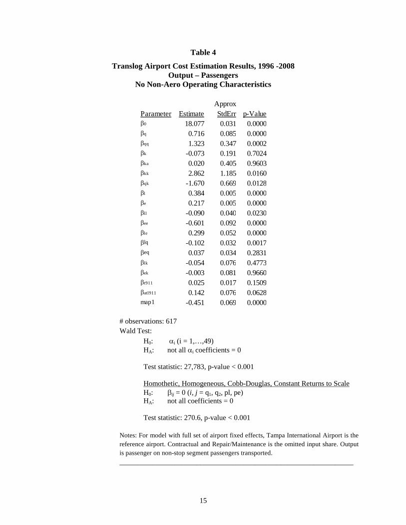
Table 4 reports the estimation results for the translog cost function, including a full set of
airport fixed effects. Relative to a general technology with no fixed effects, the Wald test
statistic, at 27,783, soundly rejects the null hypothesis that all fixed effects are zero. In addition,
estimated input shares are positive at all points and concavity conditions are satisfied at all
points, both of which are consistent with well-behaved cost functions.
V.2.1 Economies of Airport Runway Utilization
The results reported in Table 4 indicate that airports experience significant returns given
runway capacity. At the sample mean, a 1% increase in passengers transported on non-stop
15
Table 4
Translog Airport Cost Estimation Results, 1996 -2008 Output – Passengers
No Non-Aero Operating Characteristics
# observations: 617 Wald Test: H0: αi (i = 1,…,49)
HA: not all αi coefficients = 0 Test statistic: 27,783, p-value < 0.001
Homothetic, Homogeneous, Cobb-Douglas, Constant Returns to Scale H0: βij = 0 (i, j = q1, q2, pl, pe)
HA: not all coefficients = 0 Test statistic: 270.6, p-value < 0.001
Notes: For model with full set of airport fixed effects, Tampa International Airport is the reference airport. Contractual and Repair/Maintenance is the omitted input share. Output is passenger on non-stop segment passengers transported.
________________________________________________________________
ApproxParameter Estimate StdErr p-Valueβ0 18.077 0.031 0.0000βq 0.716 0.085 0.0000βqq 1.323 0.347 0.0002βk -0.073 0.191 0.7024βka 0.020 0.405 0.9603βkk 2.862 1.185 0.0160βqk -1.670 0.669 0.0128βl 0.384 0.005 0.0000βe 0.217 0.005 0.0000βll -0.090 0.040 0.0230βee -0.601 0.092 0.0000βle 0.299 0.052 0.0000βlq -0.102 0.032 0.0017βeq 0.037 0.034 0.2831βlk -0.054 0.076 0.4773βek -0.003 0.081 0.9660βt911 0.025 0.017 0.1509βatl911 0.142 0.076 0.0628map1 -0.451 0.069 0.0000
16
segments increases costs 0.72%. Alternatively, the inverse of βq, gives short run returns to
runway utilization at the sample mean, indicating that a proportionate increase in inputs increases
output 1.40%.23 However, there is quite a bit of variation in passengers (i.e. output) across
airports. For the entire sample, airports handled, on average, 9 million passengers with a 6.7
million standard deviation. Rather than evaluating at the mean, an alternative measure of returns
to runway utilization is to calculate each of these measures for each observation and then take the
average over all observations.24 This produces slightly higher returns equal to 1.64.
Disaggregating the sample by hub size found little difference in returns, 1.69 and 1.61 and for
medium and large hubs, respectively.
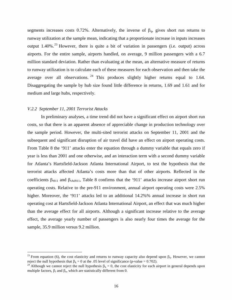
V.2.2 September 11, 2001 Terrorist Attacks
In preliminary analyses, a time trend did not have a significant effect on airport short run
costs, so that there is an apparent absence of appreciable change in production technology over
the sample period. However, the multi-sited terrorist attacks on September 11, 2001 and the
subsequent and significant disruption of air travel did have an effect on airport operating costs.
From Table 8 the ‘911’ attacks enter the equation through a dummy variable that equals zero if
year is less than 2001 and one otherwise, and an interaction term with a second dummy variable
for Atlanta’s Hartsfield-Jackson Atlanta International Airport, to test the hypothesis that the
terrorist attacks affected Atlanta’s costs more than that of other airports. Reflected in the
coefficients βt911 and βtAtl911, Table 8 confirms that the ‘911’ attacks increase airport short run
operating costs. Relative to the pre-911 environment, annual airport operating costs were 2.5%
higher. Moreover, the ‘911’ attacks led to an additional 14.2%% annual increase in short run
operating cost at Hartsfield-Jackson Atlanta International Airport, an effect that was much higher
than the average effect for all airports. Although a significant increase relative to the average
effect, the average yearly number of passengers is also nearly four times the average for the
sample, 35.9 million versus 9.2 million.
23 From equation (6), the cost elasticity and returns to runway capacity also depend upon βk. However, we cannot reject the null hypothesis that βk = 0 at the .05 level of significance (p-value = 0.702). 24 Although we cannot reject the null hypothesis βk = 0, the cost elasticity for each airport in general depends upon multiple factors, βl and βe, which are statistically different from 0.
17
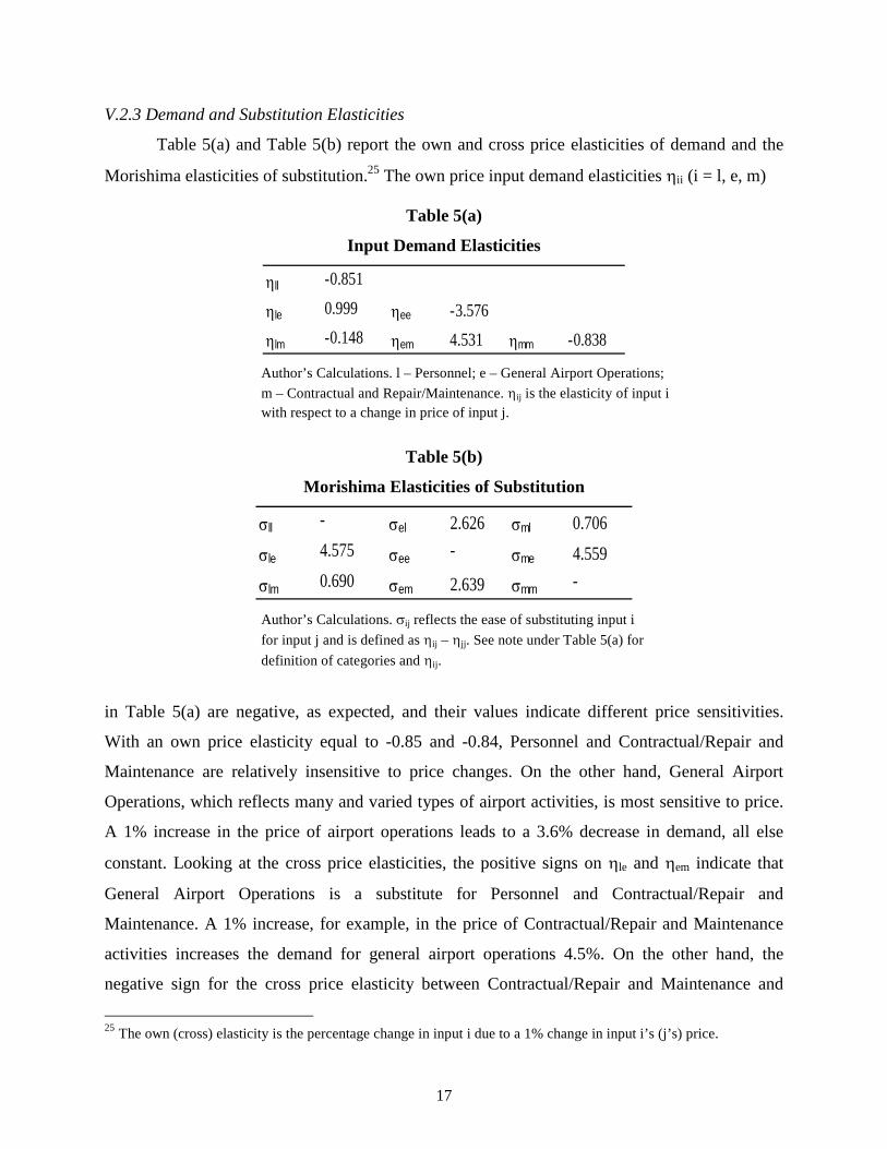
V.2.3 Demand and Substitution Elasticities
Table 5(a) and Table 5(b) report the own and cross price elasticities of demand and the
Morishima elasticities of substitution.25 The own price input demand elasticities ηii (i = l, e, m)
Table 5(a)
Input Demand Elasticities
ηll -0.851
ηle 0.999 ηee -3.576
ηlm -0.148 ηem 4.531 ηmm -0.838 Author’s Calculations. l – Personnel; e – General Airport Operations;
m – Contractual and Repair/Maintenance. ηij is the elasticity of input i with respect to a change in price of input j.
Table 5(b)
Morishima Elasticities of Substitution
σll - σel 2.626 σml 0.706
σle 4.575 σee - σme 4.559
σlm 0.690 σem 2.639 σmm -
Author’s Calculations. σij reflects the ease of substituting input i
for input j and is defined as ηij – ηjj. See note under Table 5(a) for
definition of categories and ηij .
in Table 5(a) are negative, as expected, and their values indicate different price sensitivities.
With an own price elasticity equal to -0.85 and -0.84, Personnel and Contractual/Repair and
Maintenance are relatively insensitive to price changes. On the other hand, General Airport
Operations, which reflects many and varied types of airport activities, is most sensitive to price.
A 1% increase in the price of airport operations leads to a 3.6% decrease in demand, all else
constant. Looking at the cross price elasticities, the positive signs on ηle and ηem indicate that
General Airport Operations is a substitute for Personnel and Contractual/Repair and
Maintenance. A 1% increase, for example, in the price of Contractual/Repair and Maintenance
activities increases the demand for general airport operations 4.5%. On the other hand, the
negative sign for the cross price elasticity between Contractual/Repair and Maintenance and
25 The own (cross) elasticity is the percentage change in input i due to a 1% change in input i’s (j’s) price.
18
Personnel indicates that the two inputs are complements but the low value indicates little
relationship between the two inputs.
Table 5(b) reports Morishima elasticities of substitution indicate the ease or difficulty in
substituting to serve airport passengers.26 If it is very difficult for an airport to substitute inputs,
then an increase in the price of one input will have little impact upon the input ratio and the
elasticity of substitution will be close to 0. On the other hand, if it is easy to substitute inputs,
then the elasticity of substitution will be a higher number, indicating that an airport can more
easily shift resources into another input when the price of one input increase.
With this in mind, suppose the price of labor increases 1%. From Table 5b, σel is 2.626
and σml is 0.706, which says that a 1% in the price of labor leads to a 2.6% increase in the
(General Operations/Personnel) input ratio and a 0.706% increase in the (Contractual Repair and
Maintenance/Personnel) input ratio. The 1% increase in the price of labor generates changes in
input use that ultimately lead to a higher increase in the (General Operations/Personnel) input
ratio (2.6%) than in the (Contractual Repair and Maintenance/Labor) input ratio (0.706%). The
effects of changes in the price of General Operations and in the price of Contractual and Repair
Maintenance are given in rows 2 and 3 of Table 5b and have similar interpretations.
Blackorby and Russell (1989) demonstrate that when the price of input i increases, the
relative share of input i increases if the Morishima elasticity of substitution is less than 1 and
decreases if greater than 1. From the calculated elasticities in Table 5(b), this implies that:
1. an increase in the price of labor increases the relative share of General Airport
operations and decreases the relative share of Contractual/Repair and Maintenance;
2. an increase in the price of airport operations increases the relative shares of Personnel
and Contractual/Repair and Maintenance, respectively;
3. an increase in the price of Contractual/Repair and Maintenance decreases the relative
share of and increases the relative share of General Airport Operations.
26 Blackorby and Russell (1989) demonstrate that the Allen-Uzawa measure neither reflects the ease of substitutability between inputs in production nor is informative about relative factor shares. In contrast, the Morishima measures are asymmetric, reflect ease of substitutability between inputs, and provide information on relative shares. Both measures are conditioned on compensated or constant output input demands. This is not a restrictive assumption when production technology is homothetic since elasticities and optimal output input ratios are independent of output (Blackorby, Primont, and Russell (2007)).
19
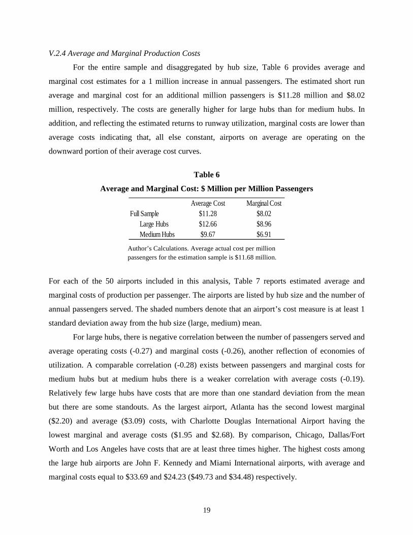
V.2.4 Average and Marginal Production Costs
For the entire sample and disaggregated by hub size, Table 6 provides average and
marginal cost estimates for a 1 million increase in annual passengers. The estimated short run
average and marginal cost for an additional million passengers is $11.28 million and $8.02
million, respectively. The costs are generally higher for large hubs than for medium hubs. In
addition, and reflecting the estimated returns to runway utilization, marginal costs are lower than
average costs indicating that, all else constant, airports on average are operating on the
downward portion of their average cost curves.
Table 6
Average and Marginal Cost: $ Million per Million Passengers
Average Cost Marginal CostFull Sample $11.28 $8.02
Large Hubs $12.66 $8.96Medium Hubs $9.67 $6.91
Author’s Calculations. Average actual cost per million passengers for the estimation sample is $11.68 million.
For each of the 50 airports included in this analysis, Table 7 reports estimated average and
marginal costs of production per passenger. The airports are listed by hub size and the number of
annual passengers served. The shaded numbers denote that an airport’s cost measure is at least 1
standard deviation away from the hub size (large, medium) mean.
For large hubs, there is negative correlation between the number of passengers served and
average operating costs (-0.27) and marginal costs (-0.26), another reflection of economies of
utilization. A comparable correlation (-0.28) exists between passengers and marginal costs for
medium hubs but at medium hubs there is a weaker correlation with average costs (-0.19).
Relatively few large hubs have costs that are more than one standard deviation from the mean
but there are some standouts. As the largest airport, Atlanta has the second lowest marginal
($2.20) and average ($3.09) costs, with Charlotte Douglas International Airport having the
lowest marginal and average costs ($1.95 and $2.68). By comparison, Chicago, Dallas/Fort
Worth and Los Angeles have costs that are at least three times higher. The highest costs among
the large hub airports are John F. Kennedy and Miami International airports, with average and
marginal costs equal to $33.69 and $24.23 ($49.73 and $34.48) respectively.

20
Table 7
Average and Marginal Cost for Large and Medium Hub Airports, 1996-2008
________________________________________________________________________________________
Authors’ calculations. For large hubs, the mean (standard deviation) for average and marginal cost is $12.7 ($9.6) and $8.9 ($6.8) respectively. For medium hubs, the mean (standard deviation) is $9.7 ($2.8) and $6.9 ($2.1) respectively. The shaded positive (negative) numbers indicate a cost measure is at least 1 standard deviation above (below) the sample mean.
Mean # Mean Mean Mean # Mean Average Mean MarginalAirport PAX Average Cost Marginal Cost Runways Cost per Runway Cost per RunwayHartsfield-Jackson International, ATL 35.85 3.09 2.20 4.23 0.73 0.52Chicago O'Hare International, ORD 29.45 11.72 8.34 6.08 1.92 1.38Dallas/Forth Worth International, DFW 25.37 10.85 7.76 7.00 1.55 1.11Los Angeles International, LAX 21.92 15.07 11.30 3.00 5.02 3.77Denver International, DEN 18.78 11.55 8.27 5.46 2.11 1.51Phoenix Sky Harbor International, PHX 18.28 5.83 4.22 2.69 2.20 1.68McCarran International, LAS 17.41 7.98 5.81 4.00 2.00 1.45Detroit Metro Wayne, DTW 15.50 12.43 8.85 7.00 1.78 1.26Minneapolis-St. Paul International, MSP 14.72 7.58 5.38 3.31 2.29 1.67Orlando International, MCO 13.60 8.37 5.98 3.46 2.42 1.76Seattle-Tacoma International, SEA 12.93 11.36 8.16 2.08 5.47 4.02Newark International, EWR 12.15 18.82 13.47 3.00 6.27 4.49Charlotte Douglas International, CLT 11.82 2.68 1.95 4.00 0.67 0.49Lambert St.Louis International, STL 11.28 7.55 3.51 5.23 1.42 0.71Philadelphia International, PHL 11.19 9.81 7.05 3.77 2.61 1.89Laguardia International, LGA 10.84 13.32 9.68 3.00 4.44 3.23General Edward Lawrence Logan, BOS 10.51 17.07 12.10 5.23 3.25 2.32Salt Lake City International, SLC 9.46 7.57 5.44 4.00 1.89 1.36Baltimore-Washington International, BWI 9.08 8.03 5.74 4.00 2.01 1.44John F. Kennedy International, JFK 8.94 33.69 24.23 4.00 8.42 6.06San Diego International, SAN 8.37 7.41 6.03 1.00 7.41 6.03Miami International, MIA 8.06 49.73 34.48 3.46 14.34 10.42Tampa International, TPA 7.84 9.29 6.77 3.00 3.10 2.26Fort Lauderdale/Hollywood International, FLL 7.49 6.68 4.47 3.00 2.23 1.49Ronald Reagan Washington National, DCA 7.47 14.01 10.22 4.00 3.50 2.55Washington Dulles International, IAD 7.44 9.78 6.40 5.00 1.96 1.28Chicago Midway International, MDW 6.74 20.45 14.12 3.08 6.65 4.61
Cincinnati/Northern Kentucky, CVG 8.52 7.04 4.57 3.31 2.11 1.46Pittsburgh International, PIT 7.19 10.38 5.83 4.00 2.59 1.46Portland International, PDX 6.43 9.98 7.21 3.00 3.33 2.40Kansas City International, MCI 5.87 8.79 6.25 3.00 2.93 2.08Cleveland-Hopkins International, CLE 5.45 9.61 6.55 4.58 2.09 1.48Memphis International, MEM 4.91 8.67 6.28 3.92 2.21 1.61Nashville International, BNA 4.65 8.88 6.44 4.00 2.22 1.61John Wayne Airport Orange County, SNA 4.57 8.76 7.44 3.00 2.92 2.48New Orleans International, MSY 4.55 6.88 4.59 3.00 2.29 1.53Sacramento Metro, SMF 4.36 12.53 9.15 2.00 6.26 4.58Raleigh-Durham International, RDU 4.15 6.93 4.98 3.00 2.31 1.66Indianapolis International, IND 3.78 14.73 10.70 3.00 4.91 3.57Dallas Love Field, DAL 3.70 4.92 3.45 3.00 1.64 1.15Austin-Bergstrom International, AUS 3.67 10.15 7.41 2.00 5.08 3.70San Antonio International, SAT 3.59 12.05 8.73 3.00 4.02 2.91Albuquerque International, ABQ 3.45 8.29 5.94 4.00 2.07 1.48Port Columbus International, CMH 3.26 13.94 9.99 2.00 6.97 4.99Bradley International Airport, BDL 3.08 9.49 6.84 3.00 3.16 2.28General Mitchell International, MKE 3.02 10.42 7.57 5.00 2.08 1.51Palm Beach International, PBI 2.98 8.40 6.12 3.00 2.80 2.04Southwest Florida International, RSW 2.83 15.02 10.78 1.00 15.02 10.78Jacksonville International, JAX 2.61 12.41 8.99 2.00 6.21 4.50Burbank Bob Hope , BUR 2.56 4.16 3.02 2.00 2.08 1.51
21
For medium hubs, the marginal cost for Cincinnati/Northern Kentucky ($5.57) is at
least one standard deviation below the mean for medium hubs. And Burbank Bob Hope
Airport has is a low cost provider ($3.02 marginal cost and $4.16 average cost) relative to the
mean. High cost medium hub airports whose average and marginal costs are well above the
medium hub mean include Sacramento is $12.53 and $9.15, Indianapolis is $14.73 and
$10.70, Port Columbus International is $13.94 and $9.99, and Southwest Florida
International is $15.02 and $10.78.
The last column in Table 7 normalizes per passenger marginal cost by runway. For large
hubs, Charlotte Douglas and Atlanta have the lowest average and marginal cost per runway,
whereas Miami has the largest average and marginal cost per runway. Among medium hubs,
Dallas Love Field has the lowest cost per runway, in comparison with Southwest Florida, which
has the highest average and marginal cost per runway.
V.2.5 Atlanta’s Hartsfield-Jackson International Airport
The previous analysis is focused upon costs and production technology for a 13 year
period for 50 large and medium hub airports. Atlanta’s Hartsfield-Jackson International Airport
is unique in this panel because of the significantly larger number of passengers served relative to
other MSAs with only one commercial airport. From a cost perspective, do Atlanta’s costs differ
significantly from other airports in the sample? Relative to the other airports included in this
study, Atlanta serves 21% more passengers than next busiest airport, Chicago’s O’Hare Airport.
Atlanta’s scale has potential cost implications that other airports face to a smaller degree.
The translog cost results reported in Table 4 confirmed this. Interacting a dummy variable for
Atlanta with the ‘911’ dummy variable and interacting an Atlanta dummy with the runway
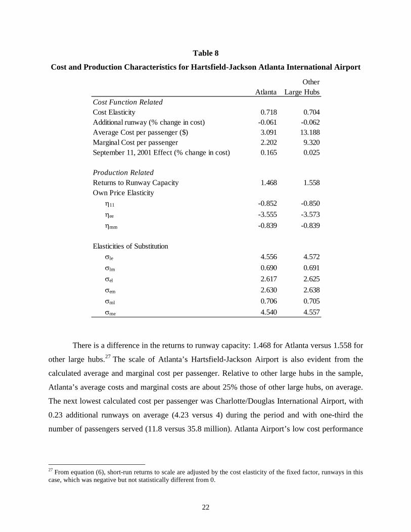
variable yield coefficients that are statistically significant at the 0.10 level. Table 8 summarizes
the cost and technological attributes for Atlanta’s Hartsfield-Jackson International Airport
relative to the other large hubs in the sample. There is virtually no difference between Atlanta
and the other large hubs in terms of input demand or factor substitution in serving airport
passengers and in the effect of an additional runway. The major differences between Atlanta and
the other large hubs center on average and marginal costs, returns to capacity, and on the ‘911’
attacks as noted above. The percentage effect of ‘911’ is more than 6 times larger relative to
other large hubs.
22
Table 8
Cost and Production Characteristics for Hartsfield-Jackson Atlanta International Airport
There is a difference in the returns to runway capacity: 1.468 for Atlanta versus 1.558 for
other large hubs.27 The scale of Atlanta’s Hartsfield-Jackson Airport is also evident from the
calculated average and marginal cost per passenger. Relative to other large hubs in the sample,
Atlanta’s average costs and marginal costs are about 25% those of other large hubs, on average.
The next lowest calculated cost per passenger was Charlotte/Douglas International Airport, with
0.23 additional runways on average (4.23 versus 4) during the period and with one-third the
number of passengers served (11.8 versus 35.8 million). Atlanta Airport’s low cost performance
27 From equation (6), short-run returns to scale are adjusted by the cost elasticity of the fixed factor, runways in this case, which was negative but not statistically different from 0.
OtherAtlanta Large Hubs
Cost Function RelatedCost Elasticity 0.718 0.704Additional runway (% change in cost) -0.061 -0.062Average Cost per passenger ($) 3.091 13.188Marginal Cost per passenger 2.202 9.320September 11, 2001 Effect (% change in cost) 0.165 0.025
Production RelatedReturns to Runway Capacity 1.468 1.558Own Price Elasticity
η11 -0.852 -0.850
ηee -3.555 -3.573
ηmm -0.839 -0.839
Elasticities of Substitutionσle 4.556 4.572
σlm 0.690 0.691
σel 2.617 2.625
σem 2.630 2.638
σml 0.706 0.705
σme 4.540 4.557

23
will likely show up in a variety of positive ways that complement Atlanta’s economic
development objectives.
VI. Discussion and Potential Implications for Economic Development
Past research on the economic development effects of airports typically explore linkages
that exist between various measures of airport output and measures of metropolitan development.
Exemplifying this approach, Goetz (1992) finds a positive correlation between per capita
passenger flows and measures of economic development growth.
From the estimated translog cost model, estimates of the average variable cost are easily
available, as reported in Table 7. With average cost estimates, one can explore whether a
relationship exists between real average costs and economic development indicators, including
real gross state product and real gross metropolitan product. The exploratory two-way fixed
effects regression model includes a separate interaction term to determine whether Atlanta
experienced any differential effects from the September 11, 2001 terrorist attacks.28
Table 9 presents the estimation results which indicate that increasing airport average
costs are related to economic development indicators. With the exception of real per capita
income, in which the effect is positive, a 1% increase in an airport’s real average cost of serving
passengers in MSAs with only one commercial airport is associated with a 0.30% reduction in
lower metropolitan employment and approximately a 0.35% decrease in metropolitan
establishments. Also consistent with the notion that an airport’s impact will have larger local
effects, Table 9 reports the finding that an increase in real average cost is associated with
reductions in real gross state product but the magnitude of the effect is lower than that that for
MSA indicators, -0.24%, versus -0.30%.
Also reported in Table 9 is an interaction term between Real Average Cost and whether
an airport is one of multiple airports in the MSA. Table 9 reports two findings. First, for each of
the economic indicators, the sign of the interaction term is positive. Second, the magnitude of the
effect is smaller than the direct effect, i.e. the effect on MSAs with one commercial airport. For
example, for airports located in a multiple airport MSA, such as Los Angeles and New York, a
28 Reported models are double-log specifications which performed better than alternative linear and other model specifications.

24
Table 9
Average Airport Operating Costs and Indicators of Economic Development, 1990 – 2008
Authors’ Calculations. All results are based on a panel of 50 large and medium hubs, 1996 – 2008. All models contain a constant term and 49 fixed effects (Tampa International Airport is the reference airport). All models are double log models estimated in SAS.
1% increase in average operating airport costs reduces metropolitan employment and the number
of establishments by 0.28% and 0.32%. Also, the ‘911-Atlanta’ interaction term identified a
positive and significant effect upon employment, the number of establishments, gross state
product for the Atlanta MSA but a decrease in real per capita income. This variable is likely
capturing more than the terrorist attacks in finding that, relative to other airports in the sample,
Atlanta experienced an increase in economic activity but not per capita incomes subsequent to
the attacks.
Building upon these results, Table 10 reports results for the relationship between real
average airport operating costs and gross metropolitan product (GMP) and its sub-categories,
which include Leisure and Hospitality, Profession and Business, Private Goods, Private Services,
Finance, and Government.
Similar to the results in Table 9, there is a negative correlation between real GMP and
real average airport cost, indicating that a 1% increase in real average cost lowers real GMP
0.31%. The effect is lower, 0.16%, for cost increases in MSAs with more than one commercial
airport.
Metropolitan Number of Real Gross Real PerExplanatory Variable Employment Establishments State Product Capita Income
Real Average Cost -0.305 -0.359 -0.244 0.029p-value <.0001 <.0001 <.0001 0.1861
Real Average Cost* 0.089 0.119 0.091 0.073Multiple Airport MSA 0.0254 0.0364 0.0221 0.0068
911 × Atlanta 0.082 0.103 0.028 -0.07129p-value 0.0004 0.0018 0.2214 <.0001
Dependent Variable

25
Table 10
Average Airport Operating Costs and Gross Metropolitan Product, 2001 – 2008
Authors’ Calculations. All results are based on a panel of 50 large and medium hubs, 2001 – 2008. All models contain a constant term and 49 fixed effects (Tampa International Airport is the reference airport). All models are double log models estimated in SAS.
Table 10 also indicates that the impact of an increase in real average costs is negatively
related to the six sub-categories of real GMP. The largest negative association (-0.464%) is for
Profession and Business and Finance and the smallest association (in absolute value) is for
Private Goods (-0.211%). However, for MSAs with more than one commercial airport, there are
distribution effects. In particular,
• the coefficients for the interaction term is negative for the Private Goods and
Government categories, reinforcing the direct effect of an increase in real average
cost on real GMP for these categories;
• the interaction coefficient for Leisure and Hospitality and Private Services is positive
but less than the direct effect which gives an overall negative relationship between
real average airport cost and real GMP for these sub-categories;
• the interaction coefficient for Profession and Business and Finance is positive and
greater than the direct effect which gives an overall positive relationship between real
average airport cost and real GMP for these sub-categories. This suggests that
concerns about reverse causality may be more serious for these sub-categories.
VII. Extensions
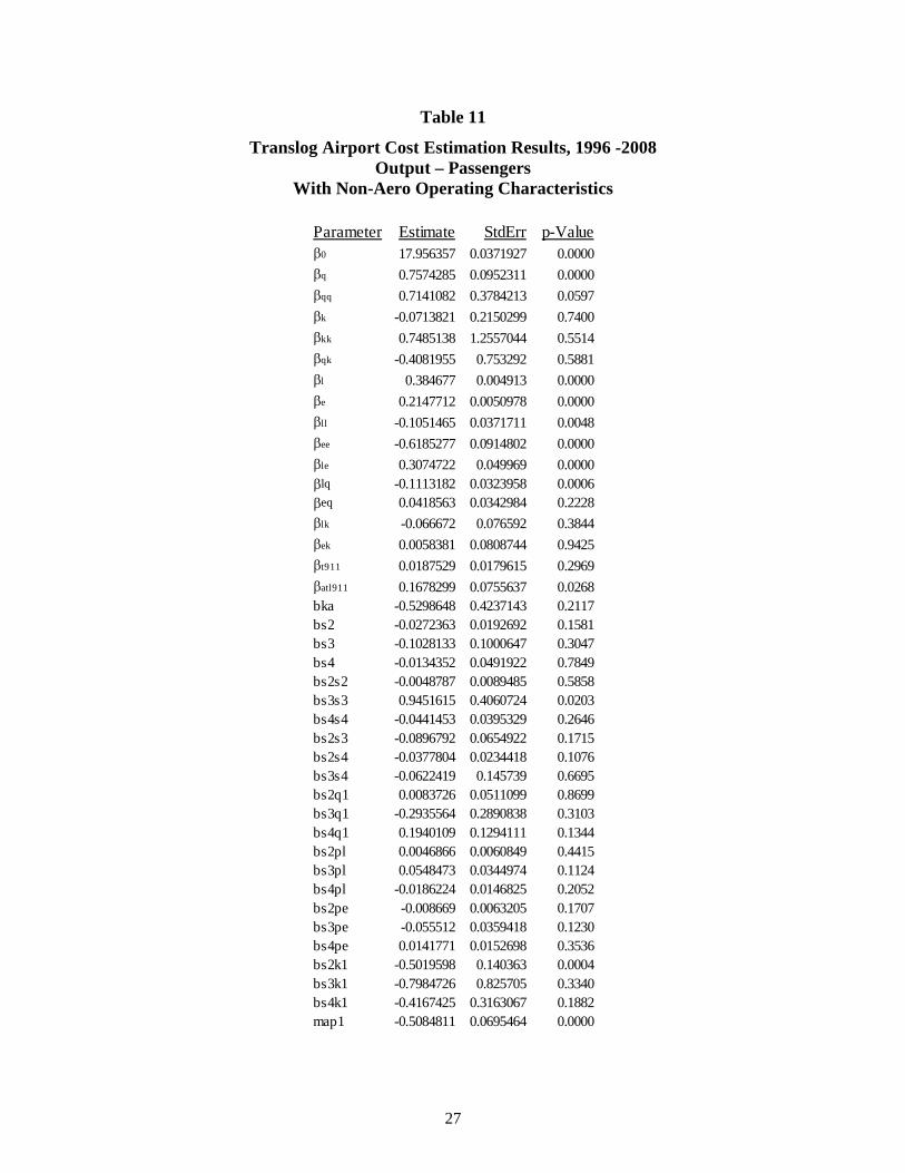
VII.1 Airport Operating Characteristics
Airports do not generate revenues solely from airline operations but also generate
revenues from complementary services and activities that airports provide to their customers.
Real Gross Real GMP Real GMP, Real GMP, Metropolitan Leisure and Profession and Real GMP, Private Real GMP, Real GMP,
Explanatory Variable Product (GMP) Hospitality Business Private Goods Services Finance Government
Real Average Cost -0.317 -0.259 -0.464 -0.211 -0.287 -0.464 -0.326p-value <.0001 <.0001 <.0001 0.0495 <.0001 <.0001 <.0001
Real Average Cost* 0.151 0.056 0.695 -0.174 0.211 0.695 -0.075Multiple Airport MSA 0.0251 0.4575 <.0001 0.2848 0.0010 <.0001 0.2890
Dependent Variable
26
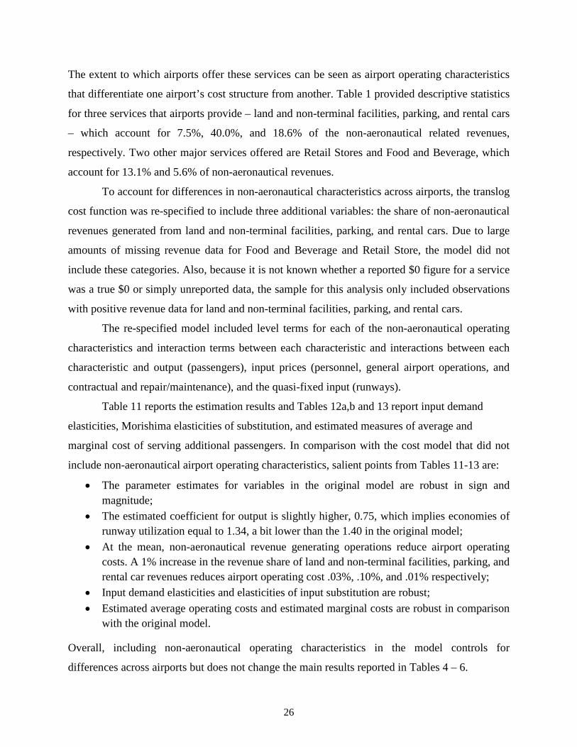
The extent to which airports offer these services can be seen as airport operating characteristics
that differentiate one airport’s cost structure from another. Table 1 provided descriptive statistics
for three services that airports provide – land and non-terminal facilities, parking, and rental cars
– which account for 7.5%, 40.0%, and 18.6% of the non-aeronautical related revenues,
respectively. Two other major services offered are Retail Stores and Food and Beverage, which
account for 13.1% and 5.6% of non-aeronautical revenues.
To account for differences in non-aeronautical characteristics across airports, the translog
cost function was re-specified to include three additional variables: the share of non-aeronautical
revenues generated from land and non-terminal facilities, parking, and rental cars. Due to large
amounts of missing revenue data for Food and Beverage and Retail Store, the model did not
include these categories. Also, because it is not known whether a reported $0 figure for a service
was a true $0 or simply unreported data, the sample for this analysis only included observations
with positive revenue data for land and non-terminal facilities, parking, and rental cars.
The re-specified model included level terms for each of the non-aeronautical operating
characteristics and interaction terms between each characteristic and interactions between each
characteristic and output (passengers), input prices (personnel, general airport operations, and
contractual and repair/maintenance), and the quasi-fixed input (runways).
Table 11 reports the estimation results and Tables 12a,b and 13 report input demand
elasticities, Morishima elasticities of substitution, and estimated measures of average and
marginal cost of serving additional passengers. In comparison with the cost model that did not
include non-aeronautical airport operating characteristics, salient points from Tables 11-13 are:
• The parameter estimates for variables in the original model are robust in sign and magnitude;
• The estimated coefficient for output is slightly higher, 0.75, which implies economies of runway utilization equal to 1.34, a bit lower than the 1.40 in the original model;
• At the mean, non-aeronautical revenue generating operations reduce airport operating costs. A 1% increase in the revenue share of land and non-terminal facilities, parking, and rental car revenues reduces airport operating cost .03%, .10%, and .01% respectively;
• Input demand elasticities and elasticities of input substitution are robust;
• Estimated average operating costs and estimated marginal costs are robust in comparison with the original model.
Overall, including non-aeronautical operating characteristics in the model controls for
differences across airports but does not change the main results reported in Tables 4 – 6.
27
Table 11
Translog Airport Cost Estimation Results, 1996 -2008 Output – Passengers
With Non-Aero Operating Characteristics
Parameter Estimate StdErr p-Valueβ0 17.956357 0.0371927 0.0000
βq 0.7574285 0.0952311 0.0000
βqq 0.7141082 0.3784213 0.0597
βk -0.0713821 0.2150299 0.7400
βkk 0.7485138 1.2557044 0.5514
βqk -0.4081955 0.753292 0.5881
βl 0.384677 0.004913 0.0000
βe 0.2147712 0.0050978 0.0000
βll -0.1051465 0.0371711 0.0048
βee -0.6185277 0.0914802 0.0000
βle 0.3074722 0.049969 0.0000βlq -0.1113182 0.0323958 0.0006βeq 0.0418563 0.0342984 0.2228
βlk -0.066672 0.076592 0.3844
βek 0.0058381 0.0808744 0.9425
βt911 0.0187529 0.0179615 0.2969
βatl911 0.1678299 0.0755637 0.0268bka -0.5298648 0.4237143 0.2117bs2 -0.0272363 0.0192692 0.1581bs3 -0.1028133 0.1000647 0.3047bs4 -0.0134352 0.0491922 0.7849bs2s2 -0.0048787 0.0089485 0.5858bs3s3 0.9451615 0.4060724 0.0203bs4s4 -0.0441453 0.0395329 0.2646bs2s3 -0.0896792 0.0654922 0.1715bs2s4 -0.0377804 0.0234418 0.1076bs3s4 -0.0622419 0.145739 0.6695bs2q1 0.0083726 0.0511099 0.8699bs3q1 -0.2935564 0.2890838 0.3103bs4q1 0.1940109 0.1294111 0.1344bs2pl 0.0046866 0.0060849 0.4415bs3pl 0.0548473 0.0344974 0.1124bs4pl -0.0186224 0.0146825 0.2052bs2pe -0.008669 0.0063205 0.1707bs3pe -0.055512 0.0359418 0.1230bs4pe 0.0141771 0.0152698 0.3536bs2k1 -0.5019598 0.140363 0.0004bs3k1 -0.7984726 0.825705 0.3340bs4k1 -0.4167425 0.3163067 0.1882map1 -0.5084811 0.0695464 0.0000

28
# observations: 617 Wald Test: H0: αi (i = 1,…,49)
HA: not all αi coefficients = 0 Test statistic: 25,890, p-value < 0.001
Homothetic, Homogeneous, Cobb-Douglas, Constant Returns to Scale
H0: βij = 0 (i, j = q1, q2, pl, pe) HA: not all coefficients = 0 Test statistic: 238.2, p-value < 0.001
Notes: For model with full set of airport fixed effects, Tampa International Airport is the reference airport. Contractual and Repair/Maintenance is the omitted input share. Output is passenger on non-stop segment passengers transported.
________________________________________

29
Table 12(a)
Input Demand Elasticities With Non-Aero Operating Characteristics
ηll -0.889
ηle 1.018 ηee -3.687
ηlm -0.129 ηem 4.663 ηmm -0.877 Author’s Calculations. l – Personnel; e – General Airport
Operations; m – Contractual and Repair/Maintenance. ηij is the elasticity of input with respect to a change in price of input j.
Table 12(b)
Morishima Elasticities of Substitution With Non-Aero Operating Characteristics
σll - σel 2.717 σml 0.763
σle 4.704 σee - σme 4.689
σlm 0.748 σem 2.735 σmm -
Author’s Calculations. l – Personnel; e – General Airport
Operations; m – Contractual and Repair/Maintenance. σij is the elasticity of substitution between inputs i and j due to a change in factor price j.
Table 13
Average and Marginal Cost With Non-Aero Operating Characteristics: $ Million per Million Passengers
Average CostMarginal Cost
Full Sample 11.37 8.53Large Hubs 12.76 9.58Medium Hubs 9.80 7.34
Author’s Calculations. Average actual cost per million passengers for the estimation sample is $11.68 million.
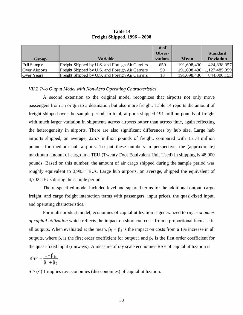
30
Table 14 Freight Shipped, 1996 – 2008
Variable
# of Obser-vations Mean
Standard Deviation
Freight Shipped by U.S. and Foreign Air Carriers 650 191,698,430 424,838,357Freight Shipped by U.S. and Foreign Air Carriers 50 191,698,4301,127,485,359Freight Shipped by U.S. and Foreign Air Carriers 13 191,698,430 844,000,153Over Years
Over Airports
GroupFull Sample
VII.2 Two Output Model with Non-Aero Operating Characteristics
A second extension to the original model recognizes that airports not only move
passengers from an origin to a destination but also more freight. Table 14 reports the amount of
freight shipped over the sample period. In total, airports shipped 191 million pounds of freight
with much larger variation in shipments across airports rather than across time, again reflecting
the heterogeneity in airports. There are also significant differences by hub size. Large hub
airports shipped, on average, 225.7 million pounds of freight, compared with 151.8 million
pounds for medium hub airports. To put these numbers in perspective, the (approximate)
maximum amount of cargo in a TEU (Twenty Foot Equivalent Unit Used) in shipping is 48,000
pounds. Based on this number, the amount of air cargo shipped during the sample period was
roughly equivalent to 3,993 TEUs. Large hub airports, on average, shipped the equivalent of
4,702 TEUs during the sample period.
The re-specified model included level and squared terms for the additional output, cargo
freight, and cargo freight interaction terms with passengers, input prices, the quasi-fixed input,
and operating characteristics.
For multi-product model, economies of capital utilization is generalized to ray economies
of capital utilization which reflects the impact on short-run costs from a proportional increase in
all outputs. When evaluated at the mean, β1 + β2 is the impact on costs from a 1% increase in all
outputs, where βi is the first order coefficient for output i and βk is the first order coefficient for
the quasi-fixed input (runways). A measure of ray scale economies RSE of capital utilization is
21
k1RSE β+β
β−=
S > (<) 1 implies ray economies (diseconomies) of capital utilization.

31
In providing air services to shippers and passengers, a question that arises is whether the
cost of providing air cargo and passenger service jointly is more or less costly than having
dedicated facilities to provide each service separately. More formally, given two outputs, q1 and
q2, economies (diseconomies) of scope are present if C(q1, q2) < (>) C(q1, 0) + C(0, q2), that is, if
the cost of joint production is less (more) than the cost of separate production.
A sufficient condition for economies of scope is weak cost complementarity, which exists
if an increase in one output lowers the marginal cost of a second output, that is, if 0qq
C
21
2
<∂∂
.
Panzar and Willig (1977) have shown that, at the sample mean, (β1β2 + β12) is an approximate
test of weak complementarity where β12 is the parameter of the interaction term.
Tables 15-18 report the parameter estimates, scale and scope economies, input and
substitution elasticities for the two output cost function model, and cost estimates. Important
findings from this model include:
• The output parameter estimate for passengers is positive and significant, reflecting passenger economies of capacity utilization. A 1% increase in passengers, all else constant, increases operating costs 0.72%;
• The output parameter estimate for freight is positive with potentially very strong freight economies of capacity utilization but the effect is not statistically significant. A 1% increase in freight shipped, all else constant, increases operating costs 0.25%;.
• The measure for ray economies of capital utilization is 1.57 which reflects production under positive economies. If all inputs are proportionately increased, passengers and freight will increase in greater proportion. Alternatively, from the cost elasticity, if passengers and freight shipped increase 1%, airport operating costs increase 0.74%, less than 1%;
• There is evidence of economies of scope, which implies that the cost joint production of passengers and cargo freight is less than the sum of separate facilities serving passengers and cargo freight, respectively, but the effect is not statistically significant;
• Estimates for input elasticity of substitution are robust relative to the single output model (with or without operating characteristics). The most sensitive substitutable input to changes in relative input prices is general airport operations;
• Input demand elasticities in the two product model were generally lower than in the single product model. In particular, for this model there is much less substitutability between ‘contractual and repair/maintenance’ inputs with personnel (from -0.148 in Table 5(a) to -0.051 in Table 17(a)) and general airport operations (from 4.531 in Table 5(a) to 1.652 in Table 17(a);

32
• The marginal cost of serving an additional passenger ranges between $1.71 and $1.75 per passenger and between $0.25 and $0.32 per pound of freight. These numbers are
33
Table 15
Translog Airport Cost Estimation Results, 1996 -2008 Output – Passengers, Freight;
With Non-Aero Operating Characteristics
ParameterEstimate p-Valueβ0 17.971 0.0000βq1 0.719 0.0000βq2 0.025 0.2275βq1q1 0.850 0.0433βq2q2 0.007 0.4031βq1q2 -0.060 0.3006βk -0.174 0.4836βkk 2.313 0.1083βq1K 0.422 0.6393βq2K -0.303 0.0525βpl 0.385 0.0000βpe 0.212 0.0000βlplpl -0.069 0.0935βlpepe -0.507 0.0000βplpe 0.243 0.0000βplq1 -0.109 0.0015βpeq1 0.063 0.0766βpeq2 0.002 0.7263βeq -0.014 0.0242βplk -0.056 0.4698βpek 0.020 0.8094βt911 0.019 0.3980βatl911 0.149 0.0408map1 -0.452 0.0000map2 -0.038 0.0173bka -0.418 0.0986βs2 -0.010 0.6460βs3 -0.041 0.7214βs4 0.036 0.5307βs2s2 -0.001 0.9020βs3s3 1.113 0.0222βs4s4 -0.016 0.7570βs2s3 -0.028 0.6885βs2s4 -0.052 0.0460βs3s4 0.005 0.9817
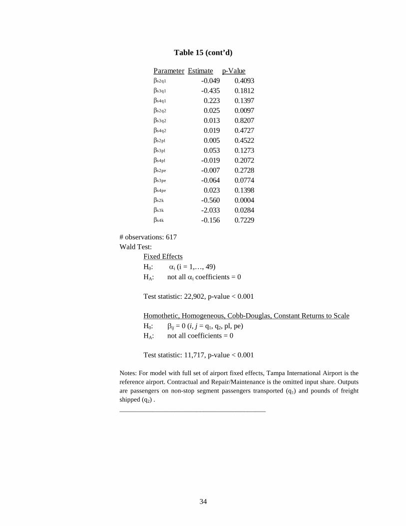
34
Table 15 (cont’d)
# observations: 617 Wald Test: Fixed Effects H0: αi (i = 1,…, 49)
HA: not all αi coefficients = 0 Test statistic: 22,902, p-value < 0.001
Homothetic, Homogeneous, Cobb-Douglas, Constant Returns to Scale H0: βij = 0 (i, j = q1, q2, pl, pe)
HA: not all coefficients = 0 Test statistic: 11,717, p-value < 0.001
Notes: For model with full set of airport fixed effects, Tampa International Airport is the reference airport. Contractual and Repair/Maintenance is the omitted input share. Outputs are passengers on non-stop segment passengers transported (q1) and pounds of freight shipped (q2) .
________________________________________
ParameterEstimate p-Valueβs2q1 -0.049 0.4093βs3q1 -0.435 0.1812βs4q1 0.223 0.1397βs2q2 0.025 0.0097βs3q2 0.013 0.8207βs4q2 0.019 0.4727βs2pl 0.005 0.4522βs3pl 0.053 0.1273βs4pl -0.019 0.2072βs2pe -0.007 0.2728βs3pe -0.064 0.0774βs4pe 0.023 0.1398βs2k -0.560 0.0004βs3k -2.033 0.0284βs4k -0.156 0.7229

35
Table 16 Two Output Model:
Economies of Scale and Scope Measures
Author’s Calculations.
Table 17(a)
Two Output Model: Input Demand Elasticities
ηll -0.795
ηle 0.846 ηee -3.187
ηlm -0.051 ηem 1.652 ηmm -0.822 Author’s Calculations.
Table 17(b)
Two Output Model: Morishima Elasticities of Substitution
σll - σel 2.335 σml 0.745
σle 4.037 σee - σme 4.063
σlm 0.771 σem 2.473 σmm -
Author’s Calculations.
Table 18 Average and Marginal Cost:
$ Million per Million Passengers, With Non-Aero Operating Characteristics
Author’s Calculations. Average actual cost per passenger and cost per pound of freight over the estimation sample is $11.68 and $2.33 respectively.
Measure Estimate p-ValueCost Elasticity 0.74 < .0000Economies of Capital Utilization 1.57 < .0000Economies of Scope -0.04 0.48
Passenger Freight Passenger FreightFull Sample 11.43 2.44 1.75 0.29
Large Hubs 12.77 2.38 1.71 0.32Medium Hubs 9.92 2.50 1.80 0.25
Average Cost Marginal Cost
36
• considerably lower than the average cost of product and reflect economies associated with capacity utilization.
The two product cost function model is a generally robust extension of the single output model
and provides additional insights into airport operating characteristics. Yet the very low output
coefficient associated with cargo freight calls for additional research to be sure that the model
appropriately captures airport cost and production characteristics and generates cost measures
that reflect airport operating environments.
VIII. Concluding Comments
Through their impacts upon regional, state, and national mobility, airports and their
associated activities can significantly benefit a metropolitan area’s economic development. Yet
relatively little is known about airport cost functions, their operational and production
characteristics.
This study’s measure of airport output is annual passengers served and cargo freight
shipped. Based upon a panel of 50 large and medium hub airports from 1996 – 2008, the
research for this paper develops and estimates flexible form translog airport operating cost
models, and this paper reports the results of three increasingly complex models: 1) one-output
(passengers) base model that does not account for non-aeronautical airport activities (e.g.
parking); 2) a one-output (passengers) model that does account for non-aeronautical airport
activities; and 3) a two-output (passengers and freight) model that accounts for non-aeronautical
airport activities. In each of these models, the number of runways is a quasi-fixed factor of
production.
The models generally fit the data well and lead to several findings that are common
across the three models:
• At the mean, airports serve passengers under increasing returns to runway capacity. All else constant, a 1% increase in passengers served increases short run operating costs between 0.71% and 0.76%;
• Reflecting economies of capacity utilization, the cost of serving additional passengers (i.e. marginal cost) is less than the average cost of serving passengers;
• An increase in runway capacity reduces short run operating costs but the effect is not statistically significant;
• Input demands for Personnel and Contractual/Repair and Maintenance are input price inelastic. All else constant, a 1% increase in the price of Personnel and
37
Contractual/Repair and Maintenance, respectively, reduces the amount of the input demanded by 0.8%;
• Input demand for General Airport Operations is input price elastic. All else constant, a 1% increase in the price of General Airport Operations reduces the amount demanded by over 3.2%;
• As a cost-minimizing response to an input price rise in General Airport Operations, airports can more easily substitute Personnel and Contractual/Repair and Maintenance inputs;
• As a cost-minimizing response to an input price rise in Personnel (Contractual/Repair and Maintenance), airports can less easily substitute Contractual/Repair Maintenance inputs (Personnel);
• The 911 terrorist attacks increased average airport operating costs 2% and Atlanta’s Hartsfield-Jackson airport costs by at least 16%;
• Airport operating costs for airports in MSA’s with more than one commercial airport (e.g. New York, Chicago, Los Angeles) were ½% lower for airports in MSAs with only one commercial airport;
• For models that included non-aeronautical activities at airports (land and terminal rentals, parking, and car rental), the mean effect was generally negative but statistically not significant.
Selected results from extensions to the base model include:
• Results from the one output model with non-aeronautical attributes were robust in comparison with the base model that did not include non-aeronautical attributes;
• For the two-output model, there are strong product economies of capacity utilization for freight shipped but the effect is not statistically significant. A 1% increase in freight shipped, all else constant, increases operating costs 0.025%.
• Airports operate under ray economies of runway capacity and economies of scope, although the measure for scope economies is not statistically significant.
How does Atlanta’s Hartsfield-Jackson airport compare with other large hubs? Although
Atlanta’s average passenger throughput is 20% higher than the next largest airport, its average
and marginal cost is at least three times less. Among the large hubs, only Charlotte Douglas
International airport, with one third the passengers in Atlanta, has lower costs. A further critical
difference between Atlanta and the other large hubs is that the 911 terrorist acts significantly
increased the airport’s operating costs.
The results also provide some evidence of an association between airport operating costs
and metropolitan economic development indicators. Increases in real airport operating costs are
associated with decreases in several indicators of economic development including real gross
38
metropolitan product. A 10% decrease in real airport operating costs, for example, is associated
with a 3.1% increase in real GMP. The results identify differential GMP effects depending upon
the sub-category of real GMP.
There are two major directions for future work in this area. First, more work is needed on
the metropolitan effects of airport operations. This analysis builds upon prior results, using a
smaller number of airports, and for the one output model provides consistent implications for
economic development. However, the relationship between economic development indicators
and real airport average costs largely disappeared in the two-output model.
A second and related direction is to conduct additional research on the two-output model.
Measures of marginal cost for passengers and freight were considerably lower than those
obtained in the one-output model. Additional work is required to assess this as well as the
economic development differences between this model and the one-output model.
IX. Acknowledgement
The Federal Aviation Administration (FAA), Contract No. DTFAWA-09-A-80021,
Georgia Department of Transportation, and the Georgia Transportation Institute-Universiyt
Transportation Center supported this research. Ms. Yuxi Xiao provided support for this project
as Graduate Research Assistant.
X. References
1. Brueckner, J. (2003) Airline Traffic and Urban Economic Development, Urban Studies 40, 1455-69.
2. Berndt, E. (1991). The Practice of Econometrics. Reading, MA: Addison-Wesley Publishing Company.
3. Brox, J.A. and C.A. Fader (2005) Infrastructure Investment and Canadian Manufacturing Productivity, Applied Economics, 37 1247-1256.
4. Caves, D.W., L., R. Christensen, and J. A. Swanson (1981) Productivity Growth, Scale of Economics, and Capacity Utilization in US Railroads, 1955-1974, American Economic Review 71(5), 994-1002.
5. Cohen, J. and C. Paul (2003) Airport Infrastructure Spillovers in a Network System, Journal of Urban Economics 54, 459-73.
6. Deno, K.T. (1988) The Effect of Public Capital on U.S. Manufacturing Activity: 1970 to 1978, Southern Economic Journal 55, 400-411.
7. Duffy-Deno, K.T. and R.W. Eberts (1991) Public Infrastructure and Regional Economic Development: A Simultaneous Equations Approach, Journal of Urban Economics 30, 329-343.
39
8. Goetz, A. (1992) Air Passenger Transportation and Growth in the U.S. Urban System, 1950-1987, Growth and Change, Spring, 217-238.
9. Green, R. (2007), Airports and Economic Development, Real Estate Economics V35, 91-112.
10. Hakfoort, J., J. Poot, and P. Rietveld (2001), The Regional Economic Impact of an Airport: The Case of Amsterdam Schiphol Airport, Regional Studies 35, 595-604.
11. Keeler, T.E. and J.S. Ying (1988), Measuring the Benefits of a Large Public Investment: the Case of the U.S. Federal-aid Highway System, Journal of Public Economics 36, 69-85.
12. Lynde, C. and J. Richmond (1992), The Role of Public Capital in Production, Review of Economics and Statistics 74, 34-44.
13. Morrison, C.J. and A.E. Schwartz (1996), State Infrastructure and Productive Performance, American Economic Review 86(5), 1095-1111.
14. Oum, T., J. Yan, and C. Yu (2007), Ownership Forms Matter for Airport Efficiency: A Stochastic Frontier Investigation of Worldwide Airports, Working Paper.
15. Panzar, J.C. and R.D. Willig (1977), Economies of Scale in Multi-Output Production, Quarterly Journal of Economics 91, 481-93.
16. Varian, H. (1984). Microeconomic Analysis (2nd Edition). New York: W.W. Norton.
Recommended