AN ABSTRACT OF THE THESIS OF
Mark J. Hauck for the degree of Master of Science in Forest Science presented on December 1, 2006. Title: Isotopic Composition of Respired CO2 in a Small Watershed: Development and Testing of an Automated Sampling System and Analysis of First Year Data Abstract approved:
Barbara J. Bond
Warming of the terrestrial biosphere due to the anthropogenic addition of carbon
dioxide to the earth’s atmosphere is becoming a major focus of scientific inquiry.
Predictions of the extent of this warming are hampered by uncertainty in the ability of the
earth’s ecosystems to counteract this effect by sequestering carbon dioxide by increases
in the mass of vegetation, soil storage, or storage in the Earth’s oceans. Measurement of
the carbon isotopic composition of respired CO2 (δ13CR-eco) is becoming increasingly
important to ecosystem studies because the information contained in this respiration can
be an indicator of ecosystem stress and productivity. This study was conducted as part of
a larger research project aimed at developing and testing the capacity for measuring
δ13CR-eco in a small, steeply-sloped watershed in western Oregon. The goals of this study
were: (1) to develop and test an automated system for sampling nocturnal air to be
analyzed in a laboratory for isotopic composition; (2) to collect samples of the

atmosphere from the nocturnal cold air drainage of a steeply sloped watershed in the HJ
Andrews Experimental Forest and bring those samples back to a laboratory to be
analyzed for CO2 concentration and carbon isotope composition; and (3) to conduct an
initial analysis of the relationship between δ13CR-eco for the first year of deployment and
two environmental forcing factors, soil moisture and atmospheric vapor pressure deficit
(VPD).
The automated system was designed during 2004 and 2005, tested in the
laboratory during the month of April 2005, debugged in the field between August 2004
and May 2005, and deployed during the period from late May, 2005 to November 2005.
The design objectives for the automated sampling system were: (1) light weight; (2)
portability; (3) high reliability; (4) fast dynamic response; (5) unattended operation; and
(6) the ability to capture, transport, and store samples over several days with no loss of
data integrity. The automated sampling system proved capable of collecting 15 samples
per sampling period and utilized a 16 loop stainless steel sample capture valve (Valcon
Instruments, 7806 Bobbitt Houston, TX 77055) for sample containment. The system was
designed for automated, labor free operation and uses a Campbell CR 10X datalogger
(Campbell Scientific, Inc, 815 West 1800 North, Logan Utah) for both data acquisition
and system control. This unique architecture was selected to enhance the ability of the
system to capture samples which could be analyzed simultaneously for both CO2
concentration and δ13C. The system was deployed in a steeply sloped watershed and
proved to have a combination of light weight (approximately 34 kg total weight) and
portability which allowed a wide range of field personnel to deploy the system without
undue physical stress. Some initial issues with electrical wiring, plumbing connections,

and control program bugs hampered early season performance, but once the system was
debugged, it functioned reliably throughout the remainder of the field season with a
minimum of operator input. Test results showed that the automated sampler had a
maximum sampling frequency of 0.043 hertz, could store air samples for up to 3 days
without detectable changes in either isotopic composition or CO2 concentration and
displayed greater precision than the hand sampling process it replaced. Using the
automated sampling system, sets of nocturnal cold air drainage samples were collected on
nine evenings in 2005. The 15 samples acquired for each of these nine evenings were
used to generate Keeling plots to determine a single value of the isotopic composition of
ecosystem respiration (δ13CR-eco) for each sampling date. The range of δ13CR-eco over the
season was 3.9 0/00 and the values of δ13CR-eco varied from -26.2 0/00 on July 13, 2005 to -
22.9 0/00 on September 14, 2005. This seasonal pattern of δ13CR-eco was consistent with a
forest under drought stress. Trends in ecosystem respiration over the growing season
were compared to corresponding measurements of the environmental variables of soil
moisture content and VPD. VPD ranged from 2.7 to 1758 Pa, but these patterns of VPD
were not significantly correlated to seasonal δ13CR-eco patterns over the study period. Soil
moisture content ranged between 7.2 % and 44.3% over the study period and soil
moisture content temporal patterns were highly correlated with rain events exceeding 4
mm. The soil moisture content pattern for the south-facing slope was significantly
correlated with the seasonal δ13CR-eco pattern, although other groupings of soil moisture
content were not.
The automated system designed for this project met all of its design objectives
and functioned adequately throughout the sampling period. The carbon isotope patterns

were consistent with a forest under drought stress and the soil moisture content of the
plots on the south-facing slopes of the watershed were significantly correlated to these
isotope patterns. The future of this system could be enhanced by making adjustments to
the supporting hardware, control program and operating procedure to enable larger
quantities of samples, more rapid sampling rates, and automated hardware diagnostics.

© Copyright by Mark J. Hauck December 1, 2006
All Rights Reserved

Isotopic Composition of Respired CO2 in a Small Watershed: Development and Testing
of an Automated Sampling System and Analysis of First Year Data
by
Mark J. Hauck
A THESIS
submitted to
Oregon State University
in partial fulfillment of the requirements for the
degree of
Master of Science
Presented December 1, 2006 Commencement June 2007

Master of Science thesis of Mark J. Hauck presented on December 1, 2006. APPROVED: Major Professor, representing Forest Science Head of the Department of Forest Science Dean of the Graduate School I understand that my thesis will become part of the permanent collection of Oregon State University libraries. My signature below authorizes release of my thesis to any reader upon request.
Mark J. Hauck, Author

CONTRIBUTION OF AUTHORS
Dr. Barbara Bond assisted with data analysis, thesis editing, and planning of the thesis
project. Dr. Thomas Pypker helped design, build, and test the automated sampling
system, assisted with data collection and analysis, and thesis editing. Dr. Elizabeth
Sulzman advised on general project issues and helped with data collection. Dr. Julia
Jones provided guidance in thesis preparation and insight on statistical issues and data
reduction. Zachary Kayler, Adam Kennedy, Aiden Padilla, Holly Barnard, Julian Licata,
and David Conklin helped with collecting data and providing encouragement and
feedback whenever needed.

TABLE OF CONTENTS
Page 1 INTRODUCTION…………………………………………………… 1 1.1 Introduction…………………………………………………. 1 1.2 References…………………………………………………… . 7 2 AN AUTOMATED SAMPLING SYSTEM FOR CAPTURING
AIR SAMPLES AT NIGHT IN REMOTE STEEPLY SLOPED, FORESTED WATERSHEDS…………………………………… 9
2.1 Abstract……………………………………………………….…. 9 2.2 Introduction……………………………………………………… 10 2.3 Background……………………………………………………… 13
2.4 Autosampler Design Issues…………………………………….. 18 2.5 System Description………………………………………………. 18
2.5 Autosampler Gas Path…………………………………………… 20 2.6 Autosampler Operation………………………………………….. 21 2.7 System Testing…………………………………………………… 23 2.8 Results……………………………………………………………. 26 2.9 Discussion………………………………………………………... 32 2.10 Conclusions…………………………………………………….. 36
2.11 Future Direction….………………………………………….…. 37 2.12 Acknowledgements and Credits………………………………… 38 2.13 Table 2.1………………………………………………….……… 39 2.14 Figures………………………………………………………..… 40 2.15 References……………………………………………………… 52 3 KEELING PLOT ANALYSIS AND ASSOCIATIONS WITH ENVIRONMENTAL VARIABLES……………..………………………. 54
3.1 Abstract………………………………………………………… 54 3.2 Introduction…………………………………………………….. … 55 3.3 Materials and Methods…………………………………….……… 58 3.4 Results……………………………………………………….……. 64 3.5 Discussion………………………………………….………..…….. 67 3.6 Conclusions………………………………………….……...……… 75 3.7 Acknowledgments and Credits………………….…………….…… 76 3.8 Figures………………………………………….……..…………… 77 3.9 References………………………………………………………… 88 4 SUMMARY AND CONCLUSIONS…………………………..…………. 92 BIBLIOGRAPY………………………………………………………….. 99


Chapter 1
ISOTOPIC COMPOSITION OF RESPIRED CO2 IN A SMALL
WATERSHED: DEVELOPMENT AND TESTING OF AN AUTOMATED SAMPLING SYSTEM AND ANALYSIS OF FIRST
YEAR DATA
Introduction:
The isotopic composition of forest ecosystem respiration (δ13CR-eco) potentially
contains a great deal of information about the metabolism of the plants inhabiting that
landscape. Although many studies have been carried out to illuminate the linkages
between ecosystem respiration and the environmental variables that influence this
metabolism (Bowling et al. 2002, Ehleringer et al. 1997), most have been aimed at sites
on flat ground, while relatively few have focused on ecosystems situated on steeply
sloped, complex terrain. While current techniques for data gathering and analysis are well
suited to flat sites with good access, the extension of these techniques to remote, steeply
sloped sites has not been advanced. Many of the world’s most productive forested
ecosystems reside on steeply sloped sites with poor access. New tools are necessary to
aid in the study of these ecosystems on complex sites. This thesis is part of a larger
project aimed at development of such tools. The goals of this thesis were: (1) to develop
and test an automated system for sampling nocturnal air to be analyzed in a laboratory for
isotopic composition; (2) to collect samples of the atmosphere from the nocturnal cold air
drainage of a steeply sloped watershed in the HJ Andrews Experimental Forest and bring
those samples back to a laboratory to be analyzed for CO2 concentration and carbon
isotope composition; and (3) to conduct an initial analysis of the relationship between

2 δ13CR for the first year of deployment and two environmental forcing factors, soil
moisture and atmospheric VPD.
The linkages between δ13CR-eco and plant physiological characteristics have been
well established (Farquhar et al., 1989, Flanagan et al., 1996). Photosynthetic
discrimination against the heavier stable carbon isotope (13C) is modulated by plant
physiological response to certain stresses, such as drought stress (Ehleringer and Cook,
1997), high salinity (Meinzer et al., 1994), lack of nutrients (Meinzer and Zhu, 1998), as
well as to high rates of assimilation (Ehleringer, 1993). Seasonal variations in isotopic
discrimination have also been reported (Buchman et al. 1997). Because the plant stores a
record of these stress states in the form of varying ratios of carbon isotopes in the sugars
fixed during photosynthesis, it is possible to relate plant tissues and plant respiration to
earlier states of stress. Furthermore, because there appears to be little or no fractionation
of isotopes of carbon after the initial photosynthetic fractionation (Lin and Ehleringer,
1997), CO2 that is respired from plants and plant ecosystems can “carry” an isotopic
signal that reflects the physiological status of plants at the point of fixation. Ekblad and
Hogberg (2001), for example, used isotopic respiration signals to demonstrate that there
was a time lag of 2 to 4 days between the time of carbon fixation and its subsequent
release from soils as respiration, with about 70% of the ecosystem respiration being
derived from those recently fixed carbon sources. This relationship has been shown to
hold in some subsequent studies of forest ecosystems (e.g., Bowling et al. 2002, Knohl,
2005) but not in others (e.g., McDowell et al. 2004).

3
In almost all previous studies of δ13CR-eco, sampling has been restricted to
relatively flat sites. This is because the analysis procedure used to determine δ13CR-eco
(described later in this thesis) requires a broad range of CO2 concentrations, and in all
previous studies this range of [CO2] has been obtained by collecting air samples through
a vertical concentration gradient that develops in still air at night on many flat sites. On
sloping sites, however, advective airflow patterns at night are likely to “break up” the
vertical gradients in CO2 concentration that are required for sampling and analyses to
determine δ13CR-eco. However, a pilot study carried out by Pypker et al. (2006, in press)
shows there is another possibility for sampling air to determine δ13CR in very steeply-
sloped areas. This study demonstrated that nocturnal cold-air drainage is a regular
occurrence in a small watershed in western Oregon. Furthermore, the concentration of
CO2 within this airflow increased substantially between dusk and pre-dawn. Thus, it is
possible in this watershed to obtain a sufficient range of [CO2] for determination of
δ13CR-eco by repetitive sampling over time rather than through a vertical gradient. The
results of Pypker et al. (2006) suggest an opportunity, for the first time, for intensive
studies of δ13CR-eco in a mountainous ecosystem.
Ecologists have developed several tools and techniques for gathering the air
samples for isotopic analysis of ecosystem respiration. Pioneering efforts in the field
include manual sampling of air in glass flasks of varying size (Ehleringer and Cook,
1997; Ometto et al., 2002; Pataki et al., 2003). These systems proved capable of
providing high quality samples but were vexed by demanding equally high quotients of
labor; workers typically need to work through the night to gather the necessary samples.

4 In order to address the issue of excessive, off-hours labor input, others (Shauer et al.,
2002; Theis et al., 2004) have developed automated sampling systems which also fill
glass flasks. These systems too have proved capable of providing high quality samples
and have addressed the labor issue handily. However, for operation in remote,
mountainous locations, these systems are too delicate due to the use of glass flasks and
too heavy to transport into these challenging sites. In addition, the large flasks are not
well suited to the Gas Bench system that is now commonly used as a front-end in isotope
ratio mass spectrometry.
A brand new technology involving tunable diode laser (TDL) systems may
eventually become the standard for all studies of isotopes in canopy air (Bowling et al.,
2003). This technology has several advantages. The analysis device is installed in situ
rather than in a laboratory. It is coupled to the sampling mechanism so that the analysis is
nearly instantaneous, avoiding the thorny transport issues associated with sampling being
separated from analysis, as in traditional flask sampled, mass spectrometer analyzed
systems. Another major advantage is that the system operates on a nearly continuous
stream of samples and thus produces data sets with large numbers of data points spanning
equally large time periods. However, TDL systems have some disadvantages associated
with them as well. At the current state of development, these systems are quite large and
heavy, making them difficult to transport to locations in rugged terrain. They also require
cryogenic cooling, which adds another level of complexity and cost. The power
requirements of a TDL system require either the use of a generator or access to line
power, both of which are prohibitive at remote sites. Given the above, although

5 tantalizing for their attributes, the disadvantages of current TDL systems make them
unsuitable at the current time for most ecosystem studies.
The attributes of a well-designed air sampling system for use in remote and
rugged locations are somewhat mutually exclusive. The ideal system would be highly
automated to preserve labor resources and prevent the fatigue associated with operator
attended all night sampling, yet be simple enough for troubleshooting and repair by a
wide range of field personnel with varying skill sets. It would be small and light, yet big
enough to be easily serviced when necessary. It would minimize power consumption to
conserve on that precious commodity that is difficult to come by in such locations, yet
have sufficient dynamic response necessary to capture samples in a rapidly changing
ecosystem. A well-designed system would be highly sensitive to changes in CO2
concentration so that the desired samples could be captured, yet rugged enough to survive
the rigors of the field conditions encountered. The system design and materials would
allow samples to be gathered and transported without introducing isotope fractionation so
as to provide high fidelity respiration data, yet not so exotic as to increase cost beyond an
acceptable limit. The system would be expandable to meet future needs and field
modifiable to adapt to changing or unanticipated conditions, yet it would be reliable so
that the stream of temporal data is not interrupted. Providing for all of these attributes
while avoiding the associated pitfalls requires making some hard choices about where to
expend resources.
This study was undertaken to address three major objectives. The first objective
was to develop an automated air sampling system to collect air samples for laboratory

6 analysis of the isotopic composition and the concentration of CO2. The second objective
was to determine, through Keeling plot analysis, the seasonal values for the isotopic
composition of ecosystem respired CO2 for a steeply sloped watershed in the HJ Andrews
research forest. The final objective was to establish whether or not relationships between
the isotopic ratio of the ecosystem respiration and the environmental variables of soil
moisture and VPD exist for this watershed. Chapter 2 of this thesis reports on the results
of the automated sampling system development while Chapter 3 presents the data that
were produced using the automated sampler as well as the analysis of those data.

7 References: Bowling DR, Sargent SD, Tanner BD, and Ehleringer JR, 2003, Tunable diode laser absorption spectroscopy for stable isotope studies of ecosystem-atmosphere CO2 exchange, Agricultural and Forest Meteorology., 118, 1-19.
Buchman N, Guehl, JM, Barigah TS, Ehleringer JR, 1997, Interseasonal comparison of CO2 concentrations, isotopic composition, and carbon dynamics in an Amazonian rainforest (French Giana), Oecologia, 110: 120-131
Ekblad A, Högberg P. 2001. Natural abundance of 13C in CO2 respired from forest soils reveals speed of link between tree photosynthesis and root respiration, Oecologia 127: 305-308 Ehleringer, JR, 1993. Variation in leaf carbon isotope discrimination in Encelia farinosa: implications for growth, competition, and drought survival, Oecologia, Volume 95, number 3
Ehleringer JR, Cook CS, 1997, Carbon and oxygen isotope rations of ecosystem respiration along an Oregon conifer transect, preliminary observations based upon small-flask sampling, Tree Physiology, 18, 513-519
Farquhar, G.D., Ehleringer, J.R., Hubick, K.T., 1989. Carbon isotope discrimination and photosynthesis. Annu. Rev. Physiol. Plant Mol. Biol., 40, 503-537
Flanagan, LB, J.R. Brooks, G.T. Varney, S.C. Berry, J.R. Ehleringer Carbon isotope discrimination during photosynthesis and the isotope ratio of respired CO2 in boreal forest ecosystems, Global Biogeochemical Cycles 96GB02345 Vol. 10 , No. 4 , p. 629
Knohl, A., Werner, R.A., Brand, W.A., Buchman, N., (2005), Short-term variations in δ
13C of ecosystem respiration reveals link between assimilation and respiration in a deciduous forest, Oecologia ,142: 70–82 Lin, G., Ehleringer, J.R., 1997, Carbon isotopic fractionation does not occur during dark respiration in C3 and C4 plants, Plant Physiology, Vol 114, Issue 1, 391-394
Meinzer, F.C., Z. Plaut, and N. Z. Saliendra, 1994, Carbon Isotope Discrimination, Gas Exchange, and Growth of Sugarcane Cultivars under Salinity, Plant Physiol. 1994 February; 104(2): 521–526
Meinzer, F.C, Zhu, J., 1998. Nitrogen Stress reduces efficiency of the C4CO2 in the concentrating system, and therefore the quantum yield, in Saccharum (sugarcane) species, Journal of Experimental Botany, Vol. 49, Number 324

8 Ometto JHB, Flanagan LB, Martinelli LA, Moreira MZ, Higuuchi N, Ehleringer JR, 2002, Carbon isotope discrimination in forest and pasture ecosystems of the Amazon Basin, Brazil, Gobal Biogeochemical Cycles, Vol. 16, No.4
Pataki DE, Ehleringer JR, Flanagan JB, Yakir D, Bowling DR, Still DJ, Buchman N, Kaplan JO, Berry JA, 2003, The application and interpretation of Keeling plots in terrestrial carbon cycle research, Global Biogeochemical Cycles, Vol 17, No.1
Pypker, T G, M H Unsworth, A C Mix, W Rugh, T Ocheltree, K Alstad and B J Bond (2006), Using nocturnal cold air drainage flow to monitor ecosystem processes in complex terrain: a pilot study on the carbon isotopic composition and advection of ecosystem respiration, in press
Schauer, AJ, Lai, CT, Bowling, DR, Ehleringer, JR, 2003, An automated sampler for collection of atmospheric trace gas samples for stable isotope analyses, Ag. And For. Meteorology (118), 113-124
Theis D, Saurer M, Blum H, Frossard E, Siegwolf TW, 2004, A portable automated system for trace gas sampling in the field and stable isotope analysis in the laboratory, Rapid Communications in Mass Spectrometry, Vol, 18, Issue 18, 2106-2112

9
Chapter 2
AN AUTOMATED SAMPLING SYSTEM FOR CAPTURING AIR SAMPLES AT NIGHT IN REMOTE STEEPLY SLOPED,
FORESTED WATERSHEDS
Abstract:
An automated sampling system was designed, built, tested and deployed in 2005
to collect samples of air for determination of the isotopic composition of ecosystem
respiration (δ13CR-eco). The design objectives for this automated system included light
weight, portability, reliability, fast dynamic response, unattended operation, and the
ability to capture, transport, and store samples over several days with no loss of data
integrity with respect to the critical measurement values of CO2 concentration and carbon
isotopic composition. The automated sampling system proved capable of collecting 15
samples per sampling period and utilized a 16 loop stainless steel sample capture valve
(Valcon Instruments, 7806 Bobbitt Houston, TX 77055) for sample containment. The
system was designed for automated, labor free operation and uses a Campbell CR 10X
datalogger (Campbell Scientific, Inc, 815 West 1800 North, Logan Utah) for both data
acquisition and system control. This unique architecture was selected to enhance the
ability of the system to capture samples, which could be analyzed simultaneously for both
CO2 concentration and δ13C. The system was deployed in a steeply sloped watershed and
proved to have a combination of light weight and portability which allowed a wide range
of field personnel to deploy the system without undue physical stress. Some initial issues
with electrical wiring, plumbing connections, and control program bugs hampered early
season performance, but once the system was debugged, it functioned reliably throughout

10 the remainder of the field season with a minimum of operator input. Test results showed
that the automated sampler had a maximum sampling frequency of 0.043 hertz, could
store air samples for up to 3 days without detectable changes in either isotopic
composition or CO2 concentration and displayed greater precision than the hand sampling
process it replaced. Using the automated sampling system, sets of nocturnal cold air
drainage samples were successfully collected on nine evenings in 2005, demonstrating
the capability of the automated system to perform as per design intent.
Introduction:
The carbon isotopic composition of forest ecosystem respiration (δ13CR-eco) is
potentially rich in information related to the health and vitality of plants inhabiting that
landscape (Flanagan et al., 1996; Flanagan et al. 1999; Fessenden et al. 2003,). There is
promise for using δ13CR-eco as a monitoring tool to evaluate ecosystem responses to
environmental variation over a range of time scales (Eckblad and Hogberg 2001;
Bowling et al. 2002). In order to capture this information efficiently and accurately, an
integrated system for field collection of samples, sample transport, and data analysis is
required. Over a two-year period, we developed such a system and methodically tested
alternate designs and procedures. This system provides an alternative sampling method
to the traditional flask samples that are frequently used to collect samples for Keeling plot
analysis (Ehleringer and Cook 1997; Shauer et al. 2003).
Charles Keeling (1958, 1961) developed a technique to identify the isotopic
composition of ecosystem-respired CO2 in samples of air collected in and above a plant

11 canopy. The Keeling method requires that samples be collected over a range of CO2
concentrations at night, when photosynthesis is not occurring. These samples are then
analyzed to determine their ratio of 13C to 12C (δ13C) and CO2 concentration. The carbon
isotopic ratio of ecosystem respiration (δ13CR-eco) is determined from this set of samples
collected over an evening using a graphical approach to solving a two end-member
mixing model (for an example of a Keeling plot, refer to Figure 2.11). To collect
samples for a single analysis (one data point), investigators have typically needed to
spend three to eight nighttime hours carefully monitoring natural fluctuations in CO2
concentrations, collecting samples in glass flasks until the required concentration range is
obtained (Ehleringer and Cook, 1997; Ometto et al., 2002; Pataki et al., 2003). The
samples are quickly returned to a laboratory for analysis to minimize the possibility of
fractionation due to slow diffusion into or out of the flask. This is a time-consuming and
expensive process, especially when the study site is remote or difficult to access.
The cumbersome method of hand collecting air samples has stimulated interest in
automating the sample collection process. Shauer et al. (2002) and Theis et al., (2004)
have developed automated sampling systems to fill gas flasks. Shauer’s automated
sampler uses a pump to move sample air through a manifold to a rotary valve. Glass
flasks with a 100ml volume are interfaced to this rotary valve. The sample gas is pumped
through one channel of the rotary valve and the valve is cycled when it is desired to
capture a sample. The valve is then sequenced to the next position and the cycle repeats
itself. Using such automated techniques allows researchers to capture samples without

12 committing field personnel to continuous duty, which minimizes the labor necessary to
get research data.
After samples are collected in the field, they are returned to the laboratory for
analysis of isotope composition. In the case of the glass flasks sampled by Shauer et al.
(2002), the samples were analyzed by withdrawing subject gases from the flasks with a
500 ml syringe and then injecting these gases into a continuous flow isotope ratio mass
spectrometer (Finnigan MAT 252 or DeltaS, Finnigan MAT, San Jose, CA), which is
preceded by a pre-condensing unit in series with a gas chromatograph column. This
process, although extremely accurate, is both time and labor intensive and is also very
costly. In order to automate the sample analysis process (thus lowering cost per sample),
many other investigators are currently using the Finnigan Gas Bench II front end for the
introduction of samples to the MAT 252 mass spectrometer. The Gas Bench II utilizes an
automated robotic arm fitted with a dual flow needle arrangement to extract samples from
vials and introduce them into the mass spectrometer. The samples are contained in glass
vials (exetainers) which are arranged in a rack. This rack is then visited sequentially by
the robotic arm and samples are introduced in that sequence to the mass spectrometer.
Thus, the data are ordered by the sequence of sample introduction and can be later
coordinated with the sample’s meta-data. The automated sampling system developed by
Schauer et al. (2002) was designed for glass flasks and this is not compatible with the
septa-topped exetainers commonly used with the Gas Bench II. For researchers who
endeavor to decrease labor expenses by automating both the sample collection and
sample analysis systems, this lack of compatibility presents a difficult dilemma.

13 The current project was initiated to develop and test an automated air sampling
system to be used as part of the HJ Andrews Airshed project. The Andrews Airshed
project started in 2002 as a pilot project to determine, among other things, if the δ13CR-eco
could be quantified in steeply sloped, forested watersheds (Pypker et al. in press). Isotope
analyses for this project were conducted in the laboratory of Dr. Alan Mix, using a Gas
Bench II system. Thus, the automated glass flask sampling system developed by Shauer
et al. (2002) was not considered a good option for this project. Instead, a new system,
which allowed automated transfer from the sample capture containers, was developed.
Background:
Several non-automated air sample collection techniques were tested during the
pilot phase of the Airshed Project (before this M.S. project was initiated). Each of these
techniques required an operator to monitor a field portable infrared gas analyzer, or
“IRGA” (LI-6252, LI-COR Inc., Lincoln, NE) in order to determine the appropriate
sample collection times. The overall objective in this decision process is to obtain
samples with the largest possible range of CO2 concentrations. During this phase of the
study, the field [CO2] measurements were used directly in Keeling plot analyses
(described in the introduction). Later, thanks to advances in laboratory analyses, the CO2
concentration was measured by the mass spectrometer concurrently with the isotopic
analysis. Because the CO2 concentration of the canopy air fluctuates rapidly, and the
infrared gas analyzer was necessarily in series with the sample collection tubes, there
could be significant differences between the measured CO2 concentration and the true

14 concentration of gas sampled in the vials. Thus, it was determined that a buffer volume
preceding the sample location was necessary to damp out these rapidly fluctuating CO2
signals.
To avoid contaminating the samples with operator respiration a “glove bag” was
used for filling the glass vials. The operator placed open vials and their caps in the bag,
which was “plumbed” to the airflow line. At a desired CO2 concentration, the operator
capped the vials by working through the plastic walls of the bag. Tests were performed
as part of the Airshed Pilot project to determine the best combination of glass vial and
septum for field sampling. It was determined that either butyl rubber or Kel-F septa
coupled to 20ml glass vials supported accurate data retrieval over time spans in excess of
24 hours and through altitude changes between sample point and analysis lab of about
500 feet (Pypker, private communication). The Gas Bench II uses a double-needle
sampling system to “sip” gas samples from vials that are capped with septa. The vials are
arranged on a grid, and the sampler is engineered to move automatically through this
grid. This is a very efficient sampling system, and it is conceptually appealing to use a
similar system to automate the collection of air samples in the field. However, the very
small hole left by a needle might result in a very minute leak, which could lead to
fractionation of isotopes in the sample. A series of tests were conducted as part of the
Airshed Pilot Project to evaluate this concern. It was discovered that, during
transportation, sample leakage from the punctured septa and associated isotopic
fractionation reduced sample fidelity. This problem was confounded when the punctured
vials were transported from the relatively high altitude of the field site to the lower

15 altitude of the laboratory. Tu et al. (2001) found similar results, with isotopic precision
decreasing by about 0.07 permil for each day that samples were stored in vials capped
with punctured septa.
The next attempt to automate the sample collection system employed the use of a
portable automated water collection system (ISCO 6712, Teledyne ISCO, Inc, 4700
Superior Street, Lincoln NE). The ISCO automated sampler uses a pump to circulate
water through the body of the sampler. When a signal from the controller indicates that a
sample should be taken, this flow is temporarily diverted to one of 99 sample vials. The
interface between these vials and the circulation system is from industry standard
needle/septa. It was thought that this device could be modified to circulate air rather than
water, which would provide the labor saving automation necessary to fill small glass vials
with air samples without the development effort necessary to design a customized
system. These vials could then be loaded into the sample tray of the Gas Bench II, where
the samples could be automatically extracted and analyzed. However, the ISCO design
did not prove to be a good candidate for use in collecting gases. There was concern that
the pumps might not move adequate volumes of air to keep the sample lines purged and
that these pumps might cause isotopic fractionation. Also, as stated earlier, piercing the
septa was shown to cause isotope fractionation. In the end, it was determined that too
much effort would have to be expended modifying the ISCO system to make it a practical
device for sample collection.
At this point in the project, attention turned to a completely different scheme for
automating sample collection that avoided the use of vials altogether. This new scheme

16 involved the use of a Valco 16 port sample collection valve (Valco E2SD16MWE,
Valcon Industries, INC, 7806 Bobbitt, Houston, TX). This valve is a specialized sample
collection valve used extensively in laboratory instruments such as mass spectrometers
and gas chromatographs. There are 16 sets of inlet and outlet ports, which are addressed
by a spring loaded indexing distribution hub. This hub seals each set of ports from the
rest of the system and opens one set at a time for sample collection. The sample passes
through the distribution hub to an inlet port. Connected between the inlet port and the
outlet port is a length of stainless steel tubing (or “loop”), which serves as the collection
volume. The sample is then passed through this tubing to the outlet port, back through the
distribution hub, and exits the collection system. When the electronic valve controller
receives a signal from the system controller to take a sample, the hub is indexed by an
electric stepper motor, isolating and sealing the particular set of inlet and outlet ports thus
trapping the sample in the loop. Sequential indexing of the distribution hub traps samples
in each set of the 15 loops, which comprise the valve. Dawson et al. (Rugh, private
communication) tested a similar sample collection scheme, but found that isotope
fractionation occurred during sample storage. However, our own initial tests showed no
indication of fractionation in the Valco valve collection. It is possible that there may have
been some residual organic cleaning compounds retained in the sample loops in the
Dawson et al. tests, which may have contributed to the fractionation signal observed. This
problem was avoided by flushing all sample loops for 48 hours with dry N2 prior to
starting fractionation testing and all subsequent field deployments.

17
Due to the highly negative impact on δ13CR-eco of large errors in measurement of
[CO2] (Zobitz et al., 2004), it was not considered adequate to rely on field measurements
of [CO2] recorded when samples were captured. The Oregon State University College of
Oceanic and Atmospheric Sciences Stabile Isotope Mass Spectrometry Facility
(OSU/COAS SIMSF) came up with a unique solution to increase the precision of
measurement of [CO2] by using the integral of the mass spectrometer voltage output
signal to determine [CO2]. This technique provided the advantage that the CO2
concentration and the isotopic signature for a particular measurement came from the
same gas volume.
The objective of this part of the thesis was to design and test an automated system
for collecting air samples based on the Valco valve to be used for isotope analyses. The
design objectives for this automated system included light weight, portability, reliability,
fast dynamic response, unattended operation, and the ability to capture, transport, and
store samples over several days with no loss of data integrity with respect to the critical
measurement values of CO2 concentration and carbon isotopic composition. Laboratory
and field testing, and their associated results, are presented. Discussion of the results and
recommendations for system improvements are also provided.

18 Autosampler Design Issues:
The design of the automated sampling system for the HJ Andrews Airshed Project
was guided by the need to provide air samples that accurately and precisely represented
the δ13CR-eco within the watershed. It was desired that the system operate automatically to
minimize labor, especially as this labor is required for sampling between 1800 and 0200
hours. The location of the pilot study sample site is somewhat remote and difficult to
access, so light weight and portability were also highly desired. Design and operation
simplicity was sought to increase the range of personnel able to deploy the system. As
this system was to be the model for future systems, which would be semi-permanently
installed to monitor ecosystem function, it was desired that this system be both flexible
and field modifiable so that it could easily be adapted to various locations.
As mentioned above, a Finnigan Gas Bench II front end was coupled to a
Finnigan Delta Plus MAT 252 mass spectrometer to analyze the air samples provided by
the automated sampling system. Typically, samples are collected in small glass vials, or
exetainers, for use on the Gas Bench II. The sample loops used in the Valco valve system
created some unique constraints on the Gas Bench system. These issues were addressed
by the laboratory technical staff, resulting in a custom interface between the sample
containment valve and the Gas Bench II inlet.
System Description:
The automated sampling system is contained in two separate enclosures, a
“Control Enclosure” and a “Sample Valve Enclosure” (Figure 2.1). Both enclosures were

19 constructed of 0.95cm marine grade plywood with overall dimensions of 61cm x 61cm x
61cm. Wood was chosen for the initial construction of the enclosures due to the ease of
field modification and low cost. As the design matures and final component choices are
made, a transition to electrical grade fiberglass enclosures would increase the durability
of the system and provide better protection of interior components.
Two enclosures were needed to separate the sample-trapping valve from the
system control components. The Sample Valve Enclosure contains the 16 port Valco
sample containment valve and its electronic controller. A 155 cm3 polycarbonate cylinder
filled with magnesium perchlorate is mounted to the outside of this enclosure and is used
to remove water from the sample stream before it enters the delicate internals of the
sample valve. All plumbing connections inside this box are 1/8” stainless steel tubing
with Swagelok fittings. The Control Enclosure contains a LI-COR 6252 infrared gas
analyzer (IRGA), a Campbell CR10X data logger (Campbell Scientific, Inc, 815 West
1800 North, Logan Utah), a six port Valco selector valve and its controller (Valcon
E2SD6MWE, Valcon Instruments, 7806 Bobbitt Houston, TX ), the sample and purge
pumps, the solenoid valves that isolate the calibration gases, and the miscellaneous
electrical connectors that are necessary to provide power and control signals to the
various devices. The Sample Valve Enclosure weighs 14.3 kg, while the Control
Enclosure weighs 20.6 kg. See Table 2.1 for a detailed list of the components, which
make up the automated sampling system.

20 Autosampler Gas Path:
The automated sampling system retrieves air samples drawn through three ¼ inch
diameter tubes that are affixed to an adjacent 37 m tower, allowing air intake from
heights of 3m, 10m, and 28m, respectively. Each of these separate tubes has a 5 micron
filter attached so that fine particulates and water droplets are removed from the air
stream. Each of these tubes enters a bulkhead fitting mounted to the Control Enclosure.
From the bulkhead fitting, 1/8” diameter nylon tubing carries the air sample to the Valco
6 port selector valve. The automated calibration gases enter the Control Enclosure in a
similar manner, running through separate solenoid valves on their route to the Valco
selector valve. The purge pump and the sample pump are also connected to the Valco
selector valve. The sample pump outlet exits the Control Enclosure through a bulkhead
fitting and connects to a 200cm3 water trap filled with magnesium perchlorate mounted to
the outside of the Sample Valve Enclosure. The outlet of the water trap is connected to
the 16 Port Valco Sample Valve through a bulkhead fitting, which is mounted to the
Sample Valve Enclosure. The output of the 16 Port Sample Valve exits the enclosure via
a bulkhead fitting and is connected to an infra-red gas analyzer (IRGA) (LI-6252, LI-
COR Inc., Lincoln, NE, USA) through a bulkhead fitting mounted to the Control
Enclosure. The output of the IRGA is exhausted to the exterior of the Control Enclosure
via another bulkhead fitting. The Campbell Data Logger, mounted inside the Control
Enclosure, receives input signals from the IRGA and sends output signals to the sample
pump, purge pump, Selector Valve, field calibration gas solenoids, and Sample Valve

21 based on the control sequence dictated by the Logger’s programming. See the schematic
diagram of the Automated Sampling System for details (Figure 2.1).
Autosampler Operation:
The Autosampler is connected to a CR10X Campbell data logger. The automated
functions of the sampling system are triggered by software written by another member of
our research team for the datalogger. This software is responsible for providing the
timing of the control signals, which activate the sample and purge pumps, selector valve,
and sample valve. Initially, the control program starts the system pumps and infrared gas
analyzer (IRGA) one hour before sunset so that the IRGA has a sufficient warm-up
period before sampling begins. During this warm-up period, a technician performs a leak
test of all of the connections of the automated sampler and the IRGA is manually
calibrated for CO2 measurements using three field calibration gases. One hour after
sunset, the control program triggers the system to begin taking samples. This typically
occurs around 9pm PST in the summer months and is intended to be coincident with the
onset of cold air drainage in the watershed. The program is parameterized by the
technician to achieve a minimum range of CO2 concentration (usually around 30ppm),
which it uses to establish set intervals of CO2 concentration for each height sampled. A
minimum of 5 minutes must pass between each sample cycle so that flushing of all
connection tubing between the sample introduction point on the tower and the sample
collection valve is assured. The air sample passes through the selector valve from the
tower tubing and is pumped by the sample pump through the water trap. From the water

22 trap, the air sample passes through the 16 Port Sample Valve and into the IRGA. The
IRGA sends a continuous CO2 concentration signal to the data logger. When a pre-
determined CO2 concentration value is achieved, the control program triggers the data
logger to signal the sample valve to index, trapping an air sample in one of its loops. The
pre-determined concentration value is a product of a calculation between two operator-
defined values in the control program. To arrive at this concentration, the desired CO2
range is divided by the number of samples at each height (the total number of samples
divided by the number of sample heights). The results of this calculation determine the
concentration that must be achieved before the sample can be collected. Once this pre-
determined concentration is achieved and the sample collection valve has indexed, the
logger then signals the selector valve to select a new height and the program repeats its
operation. A purge pump continuously purges the two tower tubes not being currently
sampled with the aim of keeping the air moving through those tubes fresh. After the loops
are filled the program progresses the system to an idle state, shutting off the pumps and
the IRGA. If all the loops are not filled by one hour before sunrise the system enters
“panic” mode. The system then sequentially fills the remaining loops regardless of the
CO2 concentration of the air. The program records the CO2 concentration (from the
IRGA) each time the Sample Valve is directed to obtain a sample, along with the time of
sample. The temperature of the interior of the Control Enclosure is also recorded to
monitor the operating temperature of the IRGA.

23 System Testing:
Testing of the automated sampling system was performed in both laboratory and
field situations to quantify the ability of the sampler to deliver high fidelity air samples.
All of the isotopic analyses for this project were performed at the OSU/COAS SIMSF
using the Finnegan MAT 252 Mass Spectrometer coupled with the automated Gas Bench
II sample introduction process. Shauer et al. (2003) performed extensive testing of
different materials of construction of their automated sampling system, looking for
isotope fractionation effects attributable to these materials. Their results indicated that
stainless steel tubing, Viton o-rings, and Valcon M grade (high density polyethelene) seal
interface materials performed well. We chose to use the materials recommended by
Shauer et al. (2003) and focused our testing on how the system performed with respect to
isotopic fractionation and leakage or diffusion of CO2 concentration. A series of
laboratory tests and field tests were conducted to determine: (1) the maximum time
samples could be retained in the system before they no longer represented the gases from
which the samples were produced; (2) the comparison of accuracy and precision of both
isotopic composition and CO2 concentration of the automated sampling system as
compared to hand sampling; (3) the system’s dynamic response; and (4) the integrity of
the system’s plumbing from week to week.
Storage Test
This test was performed in the laboratory by filling each loop of the Valco sample
storage valve (see illustration in Appendix B) with gas from a NOAA certified tank
(nominal CO2 concentration 959 ppm ±3.5ppm). This high [CO2] gas was chosen for the

24 test because it is markedly different from the ambient laboratory gas, which makes
detection of concentration changes more apparent. On each of five sequential days, three
loops were filled with gas. Each sample was taken after gas flowed through a loop at 50
± 1 ml/min for 5 minutes. The entire system was flushed with the same NOAA gas for 15
minutes prior to the test at a rate of 100 ± 1 ml/min prior to capturing samples to ensure
that no trace gases contaminated the samples. After filling three loops each day for five
days the samples were run on the MAT 252 Mass Spectrometer, with the most recently
filled loops run first.
Hand Sampling comparison to Automated Sampling
To compare the hand and automated sampling techniques we simultaneously
filled the automated sampler sample loops and glass exetainers with CO2 of known
concentration. Similar to the Storage Test outlined above, the automated sampling
system was flushed with the field calibration gas for 15 minutes prior to capturing
samples. Once the flush process was completed, gas was allowed to flow through the
automated sampling system. For each loop sampled, an exetainer glass vial was filled just
prior to capturing the loop sample by flushing the exetainer vial from the exhaust of the
automated system and then quickly attaching a cap, which contained an un-punctured
butyl rubber septa. This technique was similar to the one used in the field to capture hand
samples used in the pilot study (Pypker et al., in press).

25 Dynamic Response Test
The Dynamic Response test was performed in the field, with the automated
sampling system connected as it is during normal operation. This testing arrangement
provided realistic conditions for determining system dynamic response, including proper
length and orientation of air supply tubing, potential kinks and bends, and plugging of
inlet filters, all of which would be difficult to simulate in a laboratory setting. The
program that controls the automated sampler was modified from its field sampling form
to allow continuous operation with operator controlled valve switching. Measurements of
CO2 concentration stabilization time after switching heights were recorded for each of 4
different heights with 5 data points being taken per height. This stabilization time
represents the minimum amount of time the system must be allowed to flush for a
particular height before a sample can be captured and is an indication of how quickly the
system can respond to changes in CO2 concentration.
Weekly System Integrity Tests
During the field season, canopy gas samples were drawn each week. To be certain
that the air samples captured by the automated sampling system were not being
compromised during transport back from the field site to the laboratory, two of the
sample loops were filled with field calibration gas at the field sampling site. These loops
were filled at random with two different field calibration gases, each with different values
of CO2 concentration and isotopic ratios. The field calibration gas samples were analyzed
in the laboratory simultaneously with the rest of the field air samples. After laboratory

26 analysis of all of the samples, all of the loops were then flushed and re-filled in the
laboratory with the two field calibration gases used to fill the two loops in the field (half
the loops with one gas and half with the other). The resulting analysis of these laboratory-
filled loops provided a statistical basis for comparison of the weekly field filled loop
samples. Any large differences between the field filled loops and the laboratory filled
loops would trigger an internal investigation of the integrity of the loops or the field data.
Inspection of the standard deviation of the laboratory data would also indicate outliers,
which serve as a second check of loop integrity.
Results:
Storage Test
The mean values for δ13C of each of the timed storage samples up to 75 hours fell
within the 95% confidence interval for the NOAA gas tested, while the values for the 97-
hour samples fell just outside the same confidence interval (Figure 2.2). The CO2
concentration within the loops fell within the 95% confidence interval (within ± 7ppm) of
the NOAA gas used for the test for the entire five-day test period, although there was
some indication of a slight positive drift in [CO2] for the final two days (Figure 2.3). The
confidence interval for the NOAA gas was established by repeatedly analyzing samples
that had been flush/filled into exetainers. The 95% confidence interval values produced
by this flush/fill process are outside those provided by NOAA for the standard gas;
however, they represent a more realistic accounting of how well our mass spectrometer
can measure the concentration (or isotopic signature) of the gas in question. Thus, this is

27 a better test of the ability of the automated sampling system to retain these data over time.
In any event, it is instructive to realize that, for a given Keeling plot analysis the change
in the δ13CR-eco for a constant offset variation of ± 2ppm (the amount of variation of the
storage test values) would be about ± 0.09 0/00 (Figure 2.12). Given that the variation in
δ13CR-eco over a season is in the range of 3 0/00 and week to week changes can be as high
as 1.5 0/00, the 0.09 0/00 variation produced by this potential error in CO2 concentration is
relatively small.
Hand Sampling comparison to Automated Sampling
In all testing, whether the subject was isotopic information or CO2 concentration,
the precision of measurements from the automated sampler was consistently better than
that of the hand sampling process (Figures 2.4 to 2.7). The standard deviation of the δ13C
values varied between 0.039 to 0.093 and 0.077 to 0.3649 0/00 for the automated
sampling system and hand sampling process. The standard deviations of the CO2
concentration for the automated sampling system were 0.58 to 0.94 ppm while the
corresponding values for the hand sampling process were 1.94 to 8.63 ppm. Clearly, the
automated sampling system is capable of producing more consistent results than the hand
sampling process.
With respect to accuracy of the automated sampling system and the hand
sampling system, the picture was less clear. The results indicated that for the lower CO2
concentration samples tested, the accuracy of the hand sampling process was better for
both the isotopic signature and the CO2 concentration (Figures 2.4 and 2.5). The

28 difference between the hand sample process mean and the flush/fill sample mean was
0.27 ppm for CO2 concentration and 0.18 0/00 for δ13C while the corresponding values for
the difference between the automated sampler process mean and the flush/fill sample
mean were 7.24 ppm and -0.39 0/00, respectively. For the higher absolute CO2
concentration samples, the situation is reversed (Figures 2.6 and 2.7). For these samples,
the difference between the hand sample process mean and the flush/fill sample mean was
0.03 ppm for CO2 concentration and -1.97 0/00 for δ13C while the corresponding values
for the difference between the automated sampler process mean and the flush/fill sample
mean were 0.03 ppm and -0.05 0/00, respectively. These results are somewhat surprising
and non-intuitive. It is suspected that there may have been some errors associated with
either the experimental technique or the mass spectrometer analysis for this test. The
expected result, given that the precision of the automated sampler is clearly much higher
than that of the hand sampling system, would be that the accuracy of the automated
sampler would also be higher than that of the hand sampling process. This is especially
true when one realizes that the loops of the automated sampler are quite small in diameter
and thus don’t allow much (or any) mixing of the helium gas which pushes the sample
gas into the mass spectrometer, whereas the hand sampling process, using a concentric
needle apparatus, is quite likely to have helium diluting the sample. This dilution should
contribute to lower accuracy of the sample gas due to the drop in output voltage of the
mass spectrometer reading associated with the lower concentration, yet there is no
consistent indication that the automated sampler outperforms the hand sampling process
with respect to accuracy in this regard. Another possible explanation for this lower

29 accuracy at low concentrations is that the mass spectrometer has shown, in general,
poorer performance as the CO2 concentration drops. Again, since the output voltage of
the mass spectrometer is proportional to CO2 concentration and at concentrations below
about 350ppm this voltage signal is below 500mV (too low for stable results), it could be
that this experiment simply presents confirmation that 300ppm CO2 concentrations can’t
be accurately measured with a mass spectrometer unless a pre-conditioning stage is
employed. It is recommended that this test be repeated at the end of this field season to
establish the true increases in both accuracy and precision afforded by the automated
sampler over the hand sample process using higher CO2 concentration test gases.
Dynamic Response Test
Results of this test show that the system’s maximum response rate is about 0.043
Hz (or about one cycle every 23.5 seconds) with no tower tubing connected to the
sampler (corresponding to a zero height measurement) (Figure 2.8). As the tower tubing
length is increased, the dynamic response of the system decreases at a rate of about 0.001
Hz m-1 (the cycle time increases by 0.58 seconds per meter of tubing). The data indicate
that the resistance to air flow imposed by the small diameter internal passages of the
components of the automated sampler coupled with the large volume of the desiccant
chamber are responsible for most of the time necessary for the system to be flushed
between cycles, with the relatively large diameter tower tubing contributing little to
overall system air flow resistance. The apparent lack of linearity may be due to varying

30 resistances within each of the separate sampling tubes, various degrees of contamination
on the surface of the inlet filter or kinking of the tubing.
Weekly System Integrity Tests
On a weekly basis the isotopic signatures of the field calibration gases were
consistently within the confidence interval established in the laboratory, whereas CO2
concentrations were not (Figures 2.9 and 2.10). During the course of this field season, we
consistently had difficulty maintaining proper calibration of our CO2 concentration, due
in large part to lack of availability of a suitable NOAA standard gas. This situation
caused the lab to rely, temporarily, on using a de facto gas standard derived from a set of
ordinary, non-NOAA calibrated tanks that were calibrated using the same LI-COR 6252
that was used in the automated sampling system. These tanks were also used to fill two of
the sample loops during weekly sampling. The values for the CO2 concentration of these
field calibration gases were established on a weekly basis using the IRGA (LI-6252),
which was calibrated using a NOAA gas of known concentration (397.7 ±0.1 ppm). The
LI-COR 6252 , when working at peak capability, has a stated variance in output of ± 1
ppm (one standard deviation, as per the LI-COR 6252 specification manual). This value
shows up in the data for this experiment as the 95% confidence interval of the weekly
field calibration gas readings from the mass spectrometer and is in fair agreement with
those values (LI-COR 95% confidence interval ± 2 ppm, mass spectrometer weekly field
calibration gas laboratory readings 95% confidence interval ± 2.75 ppm). The purpose of
this test was to alert the operators and field personnel of any situations where the Valco

31 valve storage loops might be leaking or somehow damaged. The date DOY 249
(9/6/2005) is a good example of how these data might be used. On DOY 249, the isotopic
signatures of the field calibration gases were within the 95% confidence interval of the
ongoing laboratory results, but the CO2 concentration values for the field calibration
gases were significantly different from the values produce in the laboratory. This
situation, if properly illuminated, should raise concerns about either individual loop
integrity, the integrity of the entire automated sampling system, or the calibration of the
CO2 concentration of the mass spectrometer. For this case, there was no evidence to
suggest that either the individual loops were leaking or that the automated sampling
system had malfunctioned, leaving the conclusion that there were problems with the mass
spectrometer calibration. An ongoing graph depicting seasonal results along with the last
field results could work to alert those using the system that a problem exists. This is
analogous to a control chart used on automated production lines in industry and is a
standard practice at most manufacturing facilities. Although there would be some
overhead costs associated with setting up and maintaining such a practice, the effort
would be justified by the value of early detection of problematic situations. Unfortunately
for this data set, we were not able to maintain such a system and thus relied on the mass
spectrometer technician to spot such problems and to announce these issues to the group.
We were not always successful in catching problems, as witnessed by the number of field
calibration gas data points that are outside the 95% confidence interval for CO2
concentration. One goal of future work should be to devise and implement an early
problem detection control chart.

32
Discussion:
The automated sampling system designed and built for this project provided
significant advantages over previous methods of sample collection. The testing described
above, and the results of those tests, show that the automated sampling system provides
for storage of samples in the sample loops for at least three days without significant
change in [CO2] or δ13C. This is a clear advantage for researchers who endeavor to set up
such a system and then allow it to perform its function without supervision. With the
addition of a wireless interface and transmitter, the system could be made to collect data
independently and report back to the experimenter that the system is ready for retrieval. If
there were specific requirements of the dataset (say, a particular range of CO2
concentrations), the system could continue to produce and discard nightly samples until
this threshold had been reached. Once the threshold had been reached, the system could
then alert the researcher of the data capture. The ability to store the data for up to 3 days
is a significant advantage for the researcher at this point, allowing flexibility in
deployment of individuals to retrieve the samples for analysis. Also key is the ability of
the system to simply reset itself and take another set of samples after a sample event,
which again allows flexibility in achieving the desired, predetermined data thresholds.
Although the present system is not currently enabled for such operation, the addition of a
wireless interface, a transmitter, and some relatively minor programming changes would
allow such an operational scheme. The hand sampling method, which preceded this
automated system forced, at minimum, two field technicians to be present during

33 sampling for long hours under adverse conditions. Since the capture of samples under the
hand sampling system was subject to the particular operator’s skill and judgment,
significant variation could take place between data sets produced by different sets of field
technicians. The automated system does not suffer this weakness.
The results of the test comparing automated sampling to hand sampling clearly
show that the automated system has a much higher capability with respect to precision of
the dataset than that of the hand sampling process. The standard deviation of the δ13C
values varied between 0.04 to 0.09 0/00 for the automated sampling system while the
corresponding values for the hand sampling hand system were 0.08 to 0.36 0/00, which is
at minimum a two-fold increase in precision. The corresponding values for one standard
deviation of CO2 concentration were 0.58 to 0.94 ppm for the automated sampling system
and 1.94 to 8.63 for the hand sampling system, a nearly four-fold increase in precision for
the automated sampling system over the hand sampling system. Shauer et al. (1997)
report more precise values for CO2 concentration (0.2ppm) but less precision for the
isotope results (0.12 0/00) while Buchman et al. (1997) report the opposite (1ppm for CO2
concentration and 0.03 0/00 for δ13C). Both of these authors used glass flasks for sample
storage, which was not considered feasible given the objectives of our automated system.
In summary, the automated sampling system was from two to four times more precise
than the hand sampling system it replaced, was equal to or better than those of previous
automated systems, and supported the project goals of light weight and system
portability.

34
Although the accuracy of the datasets produced by the automated system appears
to only exceed that of the hand sampling process at higher CO2 concentrations, it is felt
that this result was probably in error. There is simply no reason to suspect that the value
of CO2 concentration should affect the ability of the automated sampler to accurately
reproduce the input data from either a field or laboratory test. Given that there were
significant CO2 concentration calibration issues experienced during the course of the field
season, it is likely that these results have been skewed by this variation. Unfortunately, at
the time of this writing the automated sampling system is in steady use during the current
field season and is thus not available for follow-up testing. This follow-up test should be
completed during the winter of this year when the equipment is not in use, but there is
high confidence on the part of the author that the system will prove to be at least as
accurate in data reproduction as that of the hand sampling process and will likely far
exceed that of the performance of the hand sampler. It should be noted that, by judicious
use of standard gases during the mass spectrometer analysis of the samples that the
accuracy of the results for field testing can be improved by making constant offset
adjustments in the field data to match the sample standards data. If it were to turn out in
subsequent testing that the accuracy of the automated sampling system was not adequate,
this situation could be remedied by the use of the data from the weekly field calibration
gas tests to provide the proper data offsets. Precision improvements, however, are not
impacted by manipulation of constant offsets and therefore can’t be improved by post-
analysis manipulation. For this reason, one of the most valuable advantages of the
automated sampling system over the hand sampling process is the increase in precision

35 the automated system provides. Neither Shauer et al. (1997) or Theis et al. (2004)
indicate any values for accuracy of their measurements of either δ13C or CO2
concentration, so a direct comparison of accuracy between this automated sampling
system and previous efforts is not currently possible.
The dynamic response test performed in the laboratory shows the automated
sampler can capture individual samples at a maximum rate of about 0.043 hertz, or about
23.5 seconds per sample. The time lag between each measurement is a function of the
volume of the fluid passages in the system, the flow rate of the fluids moving through the
system, and the amount of mixing which takes place between sample capture events. The
hand sampling process, due to the instability of readings of CO2 concentration produced
by the LI-COR and the response time of the operators who used that reading to determine
sample capture points, required that a large buffer volume be inserted in the fluid path to
stabilize these readings. This large buffer volume required that much longer periods of
time elapse between capturing samples (on the order of 5 minutes) to ensure that sample
mixing was not taking place and reducing the quality of individual samples. Clearly, the
automated system, which does not require a buffer volume, has a much higher capability
with respect to sample capture rate and is therefore much better equipped to respond to
environments where there is rapid fluctuation in sample content. The automated systems
described by Theis et al. (2004), Shauer et al. (1997) and Buchman et al. (1997) all use
large volume glass flasks (1/2 to 2 L) to store samples. Although no dynamic response
was reported for any of these systems, it is highly likely that their maximum sample
capture rate would be similar to the hand sampling system described thus far (about 5

36 minutes per sample). Although the current software program requires the automated
system to sample at a maximum rate of 5 minutes per cycle, the dynamic response test
results indicate that this time period could be significantly reduced, as low as 23.5
seconds per sample. This could be a significant advantage in certain environments or
where rapid sampling is desired, especially if the capability of the system to store higher
numbers of samples were increased in conjunction with this change. It was observed in
the field that that actual rate of fluctuation of CO2 concentration was both highly varied
and extremely rapid (with changes of 0.01ppm per second not uncommon). It is
suspected that these rapid changes were not based on biologically driven processes but
instead were more likely to be caused by atmospheric turbulence and the associated
mixing of the air stream. If it was desired to capture this turbulent change, a system
capable of rapid dynamic response would be desirable.
Conclusions:
The design, construction and testing of this automated sampling system was the
result of group effort aimed at increasing the quality of the data and reducing the required
labor to capture that data for the HJ Andrews Airshed Project. The system was to be
employed remotely in a steeply sloped watershed, requiring light weight, portability, and
rugged construction. It was desired to build a system that was simple to operate to
increase the range of personnel able to use the system effectively. The system needed to
be able to interface effectively to the Finnigan Gas Bench II IRMS, which is rapidly
becoming the new standard in gas measurement for isotopic analysis. It was also desired

37 to produce an automated system which could be the working model for future automated
systems which would be called upon to operate virtually independently of supervision,
having the capability to report back to researchers when it had collected samples of a
predetermined quality. The ability of the system to capture samples in a highly dynamic
environment was also sought. With regard to all of the above objectives, the automated
system which resulted from these efforts performed admirably.
Future Direction:
Although the precision improvements of the automated sampling system
described above over the hand sampling process being clearly demonstrated by
laboratory testing, some additional testing to confirm the capability of the system with
respect to dataset accuracy should be performed. It is strongly believed that the results of
this testing will confirm that the automated system is as highly accurate as it is precise.
Weekly datasets produced by this system for analysis over the course of the field
season included field calibration gases inserted in the field to verify the soundness of the
system and to help analyze system performance. It is recommended that a control chart
strategy, or a functional equivalent of the same, be implemented and tracked by both field
personnel and laboratory technicians to increase the ability of system problems to be
detected and rectified before too many questionable data are captured.
The system has proved capable of performing its intended function without
operator intervention. The system’s capacity to function independently could be
improved by increasing the number of samples the system can store, removing the 5

38 minute settling time forced between sample capture, adding wireless communication and
transmission capability, and field supply of calibration gases. Adding these components,
along with the control program modifications necessary to make them function
seamlessly, would extend the utility of the system to new environments.
Acknowledgements and Credits:
Tom Pypker and Bill Rugh were invaluable for their assistance in design,
construction and testing of the automated sampler. Tom spent many hours in the field
helping with both sample collection and system debugging as well as explaining various
aspects of the overall project, the effort for which I am eternally grateful. Bill did the
majority of the analysis of the mass spectrometer data, often working late nights and
weekends to complete the analysis on time. The concept for the project was born from the
work on the Pilot Project for the HJ Andrews Airshed Project under the direction of Dr.
Barbara Bond, along with Co-Principle Investigators Dr.’s Elizabeth Sulzman, Michael
Unsworth, and Alan Mix. General advice and assistance were given by Zachary Kayler,
Holly Barnard, and Nicole Czarnomski.

39
Table 2.1: Autosampler Materials of Construction List Item Qnty Description Manufactur
er Model
Gas Analyzer
1 Infrared Gas Analyzer; provides control signal of CO2 concentration to system controller
LI-COR LI-6252
Selector Valve
1 6 port Selector Valve; provides selectable path for multiple source air samples
Valcon E2SD6 MWE
Sample Valve
1 16 Port Sample Valve; provides sealed storage for air samples
Valcon E2SD1 6MWE
Data Logger
1 System Controller/Data Logger; provides control signals to various system components and stores critical data
Campbell Scientific
CR 10X
Water Trap
1 155 cm3 magnesium perchlorate cylinder which traps water to keep IRGA and Sample Valve free of contamination
Sample Pump
1 Air pump; motive force for moving air samples through system
Neuberger, Inc
UNMP50 -KNDC, 12vdc
Purge Pump
1 Air pump; motive force for keeping tower sample lines purged
Brailsford TD-42N, 12vdc
Solenoid Valve
2 Isolates field calibration gas cylinders from Selector Valve
Cole Parmer 625E
Inlet Filter 3 5 µm prefilters; removes fine contaminants and water drops from incoming air samples
Bulkhead Fitting
9 Stainless steel tubing fittings; interface between inside and outside of both enclosures
Swag-Lok
Nylon Tube
Various lengths
Connects bulkhead fittings of both Enclosures and interior air sample paths in Control Enclosure
Stainless Tube
Various Lengths
Connects Sample Valve to bulkhead fittings inside the Sample Valve Enclosure
Solid State Relays
6 Relays between control signals and high power requirement components
Crydom D1D07
Inverter 1 Converts 12vdc to 110vac for Valcon Valve controllers
Radio Shack 300W High Eff., Cat # 22-146

40
Figure 2.1: Autosampler System Diagram

41
Figure 2.2
Results from a storage test performed in the laboratory. Three loops of the Valco sample storage valve (see Appendix B, Autosampler System Diagram) were filled each day for 5 days with a NOAA certified gas (nominal CO2 concentration 958.9 ppm). After the final fill process, the contents of all of the loops were analyzed using the COAS mass spectrometer.
δ13C Storage in Automated Sampler
storage time, hours
0 20 40 60 80 100 120
δ13 C
, per
mil
-24.40
-24.35
-24.30
-24.25
-24.20
-24.15
Shaded area: mean NOAA test gas plus or minus 2 standard deviations (95% C.I.)

42
Figure 2.3
Results of a storage test performed in the laboratory. Three loops of the Valco sample storage valve (see Appendix B, Autosampler System Diagram) were filled each day for 5 days with a NOAA certified gas (nominal CO2 concentration 958.9 ppm). After the final fill process, the contents of the loops were analyzed for CO2 concentration and δ13C ratio. The contents of the loops filled last represent day 0, the CO2 concentration reported for that time period was adjusted to agree with the nominal value of the NOAA gas. All of the values for the other days were adjusted using the same offset required to bring the day 0 value to alignment with the NOAA standard.
[CO2] Storage in Automated Sampler
storage time, hours
0 20 40 60 80 100 120
[CO
2], p
pm
950
955
960
965
970Shaded Area: mean NOAA test gas plus or minus2 standard deviations (95% C.I.)

43
Figure 2.4
Comparison of the isotopic accuracy and precision of two sampling techniques (autosampler and hand sampling). The test used a reference gas to fill both the autosampler loops and the hand sampled exetainer glass vials. The “flush/fill” values represent the best technique available for determining the true value of δ13C ratio of the reference gas and thus are used in this instance as a standard of comparison (“truth”).
δ13C measurements for low CO2 concentration samples June 28, 2005
data source
autosampler hand sampler flush/fill samples
δ13C
, per
mil
-10.6
-10.5
-10.4
-10.3
-10.2
-10.1
-10.0
-9.9
-9.8

44
Figure 2.5
Comparison of the performance of the automated sampler to hand sampling for capture of CO2 concentration. The test uses a field calibration gas to fill both the autosampler loops and the hand sampled exetainer glass vials. The “flush/fill” values represent the best technique available for determining the true value of δ13C ratio and CO2 concentration for a given gas and thus are used in this instance as a standard of comparison (“truth”). As can be seen from the data above, the precision of the Automated Sampling System data is much better than that of the hand sampling technique, although it appears that the hand sampling output has higher accuracy.
CO2 concentration data for low CO2 concentration samples June 28th, 2005
data source
autosampler hand sampler flush/fill samples
[CO
2], p
pm
296
298
300
302
304
306
308

45
Figure 2.6
Comparison of the performance of the automated sampler to hand sampling for capture of δ13C ratio. The test uses a field calibration gas to fill both the autosampler loops and the hand sampled exetainer glass vials. The “flush/fill” values represent the best technique available for determining the true value of δ13C ratio and CO2 concentration for a given gas and thus are used in this instance as a standard of comparison (“truth”). As can be seen from the data above, both the precision and accuracy of the Automated Sampling System data is much better than that of the hand sampling technique.
δ13C measurements for high CO2 concentration samples June 28, 2005
data source
autosampler hand sampler flush/fill samples
δ13C
, per
mil
-40.5
-40.0
-39.5
-39.0
-38.5
-38.0
-37.5
-37.0

46
Figure 2.7
Comparison of the performance of the automated sampler to hand sampling for capture of CO2 concentration. The test uses a field calibration gas to fill both the autosampler loops and the hand sampled exetainer glass vials. The “flush/fill” values represent the best technique available for determining the true value of δ13C ratio and CO2 concentration for a given gas and thus are used in this instance as a standard of comparison (“truth”). From the above results, for this test the accuracy of both techniques was extremely high while the precision of the automated sampling system far exceeded that of the samples taken by hand.
CO2 concentration data for high CO2 concentration samples June 28th, 2005
data source
autosampler hand sampler flush/fill samples
[CO
2], p
pm
436
438
440
442
444
446
448
450
452
454
456
458
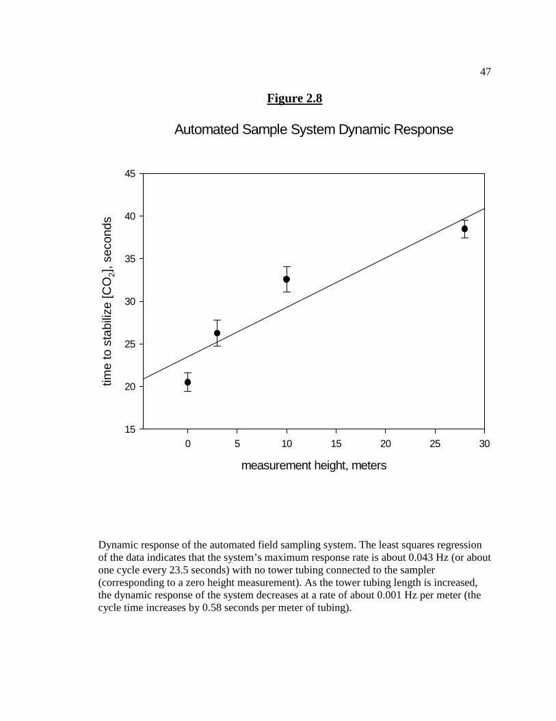
47
Figure 2.8
Automated Sample System Dynamic Response
measurement height, meters
0 5 10 15 20 25 30
time
to s
tabi
lize
[CO
2], s
econ
ds
15
20
25
30
35
40
45
Dynamic response of the automated field sampling system. The least squares regression of the data indicates that the system’s maximum response rate is about 0.043 Hz (or about one cycle every 23.5 seconds) with no tower tubing connected to the sampler (corresponding to a zero height measurement). As the tower tubing length is increased, the dynamic response of the system decreases at a rate of about 0.001 Hz per meter (the cycle time increases by 0.58 seconds per meter of tubing).

48
Figure 2.9
Differential δ13C values of the weekly field filled plumbing integrity test. Each week two separate gases which were used to field calibrate the automated sampler IRGA were stored in two loops of the sample collection valve. After the mass spectrometer analysis of all of the field samples were completed, ½ of the loops were refilled with each of these two gases. The results of the field filled loops were compared to the average of the lab filled loops of the same gas (the comparison is a differential value). The shaded portion of the graph represents the 95% confidence interval for the lab filled loops using the pooled standard deviation for these data throughout the season.
Weekly Span Gas Field Filled Trap Data for δ13C
DOY
180 200 220 240 260 280 300
δ13C
, pe
rmil
-3
-2
-1
0

49
Figure 2.10
Differential [CΟ2] values of the weekly field filled plumbing integrity test. Each week two separate calibration gases which were used to field calibrate the automated sampler IRGA were stored in two loops of the sample collection valve. After the mass spectrometer analysis of all of the field samples were completed, ½ of the loops were refilled with each of these two calibration gases. The results of the field filled loops were compared to the average of the lab filled loops of the same calibration gas (the comparison is a differential value). The shaded portion of the graph represents the 95% confidence interval for the lab filled loops using the pooled standard deviation for these data throughout the season.
Weekly Span Gas Field Filled Trap Data for CO2 Concentration
DOY
180 200 220 240 260 280 300
[CO
2], p
pm
-20
-10
0
10
20
30
40
50
60

50
Figure 2.11
Typical Keeling plot. Data from August 10, 2005.
Keeling Plot of Airshed Tower DataAugust 10, 2005
1/[CO2]
0.0021 0.0022 0.0023 0.0024 0.0025 0.0026 0.0027
δ13C
-12
-11
-10
-9
-8
-7Ordinary Least Squares Regression Resultsδ13Ceco = -28.64 + 7967.5 [CO2], r
2= 0.9518

51
Figure 2.12
Keeling plot variation with constant CO2 offset. A constant offset variation of the CO2 concentration of ± 2 ppm causes the value of δ13CR-eco to vary from -28.73 to -28.55 0/00, with the center value of -28.64 (corresponding to 0 offset).
Keeling plot variation with constant offset of CO2 concentration of +/- 2 ppm
1/[CO2]
0.0021 0.0022 0.0023 0.0024 0.0025 0.0026 0.0027
δ13C
-12
-11
-10
-9
-8
-7

52 References: Bowling, D.R., McDowell, N.G., Bond, B.J., Law, B.E., Ehleringer, J.R., 13C content of ecosystem respiration is linked to precipitation and vapor pressure deficit, Oecologia (2002), 131:113-124
Buchman N, Guehl, JM, Barigah TS, Ehleringer JR, 1997, Interseasonal comparison of CO2 concentrations, isotopic composition, and carbon dynamics in an Amazonian rainforest (French Giana), Oecologia, 110: 120-131
Ekblad A, Högberg P. 2001. Natural abundance of 13C in CO2 respired from forest soils reveals speed of link between tree photosynthesis and root respiration, Oecologia 127: 305-308
Ehleringer JR, Cook CS, 1997, Carbon and oxygen isotope rations of ecosystem respiration along an Oregon conifer transect, preliminary observations based upon small-flask sampling, Tree Physiology, 18, 513-519
Fessenden, JE, Ehleringer, JR, 2003, Temporal variation in δ13C of ecosystem respiration in the Pacific Northwest: links to moisture stress, Oecologia 136:129-136
Flanagan, LB, J.R. Brooks, G.T. Varney, S.C. Berry, J.R. Ehleringer Carbon isotope discrimination during photosynthesis and the isotope ratio of respired CO2 in boreal forest ecosystems, Global Biogeochemical Cycles 96GB02345 Vol. 10 , No. 4
Flanagan, L.B., Kubien, D.S., Ehleringer, J.R., 1999, Spatial and temporal variation in the carbon and oxygen stable isotope ratio of respired CO2 in a boreal forest ecosystem, Tellus B, Vol 51
Keeling CD, 1958, The concentration and isotopic abundances of atmospheric carbon dioxide in rural areas, Geochim Cosmochim Acta. 13: 322-334
Keeling CD, 1961, The concentration and isotopic abundance of carbon dioxide in rural and marine air, Geochim Cosmochim Acta. 24: 277-298
Miller JB, Tans PP, White JWC, Conway TJ, Vaughn BW, 2003, The atmospheric signal of terrestrial carbon isotopic discrimination and its implication for partitioning carbon fluxes, Tellus 55B, 197-206
Ometto JHB, Flanagan LB, Martinelli LA, Moreira MZ, Higuuchi N, Ehleringer JR, 2002, Carbon isotope discrimination in forest and pasture ecosystems of the Amazon Basin, Brazil, Gobal Biogeochemical Cycles, Vol. 16, No.4

53 Pataki DE, Ehleringer JR, Flanagan JB, Yakir D, Bowling DR, Still DJ, Buchman N, Kaplan JO, Berry JA, 2003, The application and interpretation of Keeling plots in terrestrial carbon cycle research, Global Biogeochemical Cycles, Vol 17, No.1
Schauer, AJ, Lai, CT, Bowling, DR, Ehleringer, JR, 2003, An automated sampler for collection of atmospheric trace gas samples for stable isotope analyses, Ag. And For. Meteorology (118), 113-124
Theis D, Saurer M, Blum H, Frossard E, Siegwolf TW, 2004, A portable automated system for trace gas sampling in the field and stable isotope analysis in the laboratory, Rapid Communications in Mass Spectrometry, Vol, 18, Issue 18, 2106-2112
Trolier M, White JWC, Tans PP, Masarie KA, Gemery PA, 1996, Monitoring the isotopic composition of atmospheric CO2: Measurements from the NOAA Global Air Sampling Network, J. Geophy. Res., Vol. 101, No. D20
Tu KP, Brooks PD, Dawson TE. 2001. Using septum-capped vials with continuous-flow isotope ratio mass spectrometric analysis of atmospheric CO2 for Keeling plot applications. Rapid Commun. Mass Spectrom.15:952–56
Zobitz JM, Keener JP, Bowling DR, 2004, Sensitivity analysis and quantification of uncertainty for isotopic mixing relationships in carbon cycle research, American Geophysical Union, Fall Meeting 2004, in press

54
Chapter 3
KEELING PLOT ANALYSIS AND ASSOCIATIONS WITH ENVIRONMENTAL VARIABLES
Abstract: Variation in the isotopic composition of ecosystem respiration (δ13CR-eco ) was
studied over the 2005 growing season at Watershed 1 of the HJ Andrews Experimental
Forest in western Oregon with the goal of understanding relationships between
environmental factors, especially atmospheric humidity and soil moisture, and δ13CR-eco.
The watershed has a pronounced nocturnal air drainage system, and concurrent
atmospheric studies have revealed that the air passing the tower at night contains a well-
mixed sample of respired CO2 from the entire 96 ha basin. Samples of air were collected
at night from various heights of a 37m tower erected at the base of the watershed on nine
occasions between July 13, 2005 and October 5, 2005.The automatic sampler collected
15 air samples for each sampling period, and the concentration and carbon isotope
composition of CO2 in these samples was determined in the COAS laboratory at Oregon
State University. δ13CR-eco was determined from these measurements using the Keeling
Plot approach. Instrumentation affixed to the tower continuously measured microclimatic
conditions during the study period; microclimate as well as soil moisture was also
continuously monitored along a transect of eight plots arrayed across the watershed.
Measured values of δ13CR-eco increased from -26.2 0/00 on 13th of July to -22.9 0/00 on 14th
of September. VPD, measured by instruments affixed to the tower and averaged over 24
hour periods, ranged from 2.7 to 1758 Pa, but VPD patterns were not correlated to

55 seasonal δ13CR-eco patterns over the study period. Soil volumetric water content ranged
between 7.2 % and 44.3% over the study period; the variation in soil volumetric water
content over the study period was highly correlated with rain events exceeding 4 mm.
Soil volumetric water content on south-facing slopes was significantly correlated (r = -
0.77, p < 0.01) with seasonal δ13CR-eco.
Introduction:
Ecosystem scientists have developed many methods and tools to study metabolic
processes of forested ecosystems on flat terrain. Remote sensing (Martin et al. 1997),
micrometeorology (Baldocchi 1997; Yakir et al. 2000; Baldocchi 2003), and flask
sampling of air (Buchmann et al. 1998; Bowling et al. 2001) have been used successfully
to uncover important ecosystem functions on flat land, but most of these techniques are
inadequate when addressing ecosystem processes for forests lying on mountainous
terrain. Micrometeorological techniques (eddy covariance) require a homogenous forest
where horizontal fluxes of mass and momentum sum to zero over short timescales. In
complex terrain, advection of air into the system via nighttime cold air drainage violates
this requirement, thereby introducing unacceptable levels of uncertainty (Black et al.
1996, Lavigne et al. 1997, Staebler and Fitzjarrald 2004). Due to the inherent difficulty in
studying forested systems in mountainous terrain, these systems are poorly represented in
the scientific literature. As some of the most productive ecosystems in the world lie on
such terrain (Harmon et al. 2004), the study of ecosystem metabolism and associated
environmental conditions are among today’s most important ecological problems
(Schimel et al. 2002).

56
Convection and advection account for much of the air movement in areas with
mountainous terrain. Disproportionate heating of air by radiative energy from sunlight at
the ridge of a mountain during the day causes that air to rise (convection), lowering local
pressure. Air from the valley flows into this low pressure zone and an up-valley wind
results. During the nighttime hours, radiative cooling of the surface of the slopes in this
terrain causes local air temperature to decrease, which increases that air’s density.
Gravity then drives this air down the slope, creating down slope winds. Air from above
the valley surface moves in (advection) to replace this lost air, setting up airflow patterns
that mimic stream flows. This airflow is strongest on cloudless nights, when radiative
losses are highest (Monteith and Unsworth 1990). This nighttime airflow pattern in
mountainous terrain has been termed “cold air drainage” (Fleagle 1950, Manins and
Sawford 1979, Mahrt and Larsen 1982, Whiteman 1990).
Nocturnal cold air drainage flows entrain any gases released by the vegetation and
soils on the slopes of the mountainous terrain. Of particular interest to ecosystem
scientists studying the carbon cycle in mountainous regions is the capture and transport of
respired CO2 from vegetation and soils. Environmental variables such as VPD,
temperature, and soil moisture have been linked to the isotopic composition of this
ecosystem respiration (Bowling et al. 2002, Barbour et al. 2005, Ekblad and Hogberg
2001). The isotopic composition of respired CO2 varies as a result of discrimination
against the heavier isotope of carbon by vegetation during photosynthesis (Farquhar et al.
1989, Ehleringer et al. 1992). As a result of this discrimination, the respiration of plants
and soils are depleted in 13C (Pataki et al. 2003), and this respiration appears to be
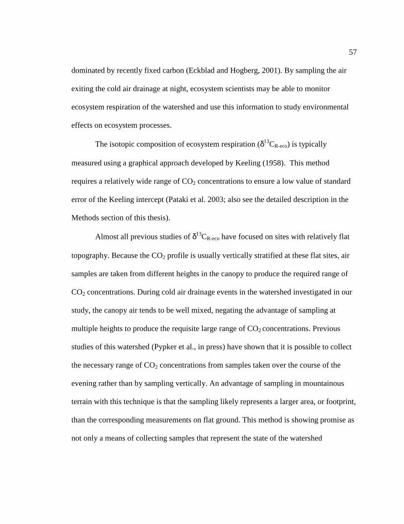
57 dominated by recently fixed carbon (Eckblad and Hogberg, 2001). By sampling the air
exiting the cold air drainage at night, ecosystem scientists may be able to monitor
ecosystem respiration of the watershed and use this information to study environmental
effects on ecosystem processes.
The isotopic composition of ecosystem respiration (δ13CR-eco) is typically
measured using a graphical approach developed by Keeling (1958). This method
requires a relatively wide range of CO2 concentrations to ensure a low value of standard
error of the Keeling intercept (Pataki et al. 2003; also see the detailed description in the
Methods section of this thesis).
Almost all previous studies of δ13CR-eco have focused on sites with relatively flat
topography. Because the CO2 profile is usually vertically stratified at these flat sites, air
samples are taken from different heights in the canopy to produce the required range of
CO2 concentrations. During cold air drainage events in the watershed investigated in our
study, the canopy air tends to be well mixed, negating the advantage of sampling at
multiple heights to produce the requisite large range of CO2 concentrations. Previous
studies of this watershed (Pypker et al., in press) have shown that it is possible to collect
the necessary range of CO2 concentrations from samples taken over the course of the
evening rather than by sampling vertically. An advantage of sampling in mountainous
terrain with this technique is that the sampling likely represents a larger area, or footprint,
than the corresponding measurements on flat ground. This method is showing promise as
not only a means of collecting samples that represent the state of the watershed

58 respiration signal, but as well a method to monitor ecosystem processes within a steeply
sloped watershed.
The goal of this study was to investigate the relationships between the isotopic
concentration of ecosystem respiration and two important environmental factors that
affect carbon isotope discrimination by plants: VPD and soil volumetric water content.
The specific objectives were to: (1) use an automated sampling system to produce weekly
samples of air for isotopic and CO2 concentration laboratory analysis; (2) determine
weekly values of δ13CR-eco from the results of these laboratory analyses; (3) attempt to
correlate this pattern of δ13CR-eco to the environmental variables of VPD and soil
volumetric water content.
Materials and Methods:
Study Site
All measurements were made in Watershed #1 (WS1) of the HJ Andrews
Experimental Forest in the western Cascades of central Oregon, USA (44.2 °N, 122.2
°W). This watershed covers 96 ha and was harvested in the late 1960s. Douglas-fir
(Psuedostuga menziessii) dominates this closed canopy forest, with secondary
components of bigleaf maple (Acer macrophyllum), red alder (Alnus rubra) and western
hemlock (Tsuga hererophylla). This site is typical of those in the western Cascades, with
wet, mild winters and warm, dry summers. The soils of this watershed are gravelly clay
loams (Swanson and James 1975). A 37m tower was erected at the base of this watershed
to serve as the focal point for collection of air samples and meteorological data. A

59 transect consisting of eight plots was installed across the watershed slightly upstream
from the tower and normal to the stream, which generally follows a northwesterly path.
The plots are identified by numbers; plots 501, 502, 504 and 505 are arrayed from the
ridge top to the lower slope of the southwest-facing side of the watershed and plots 507,
508, 510 and 512 are arrayed from the lower slope to the ridge top of the northwest
facing slope (the numbering system was established to correspond to nearby long-term
vegetation plots. The discontinuity in the numbers occurs because not all of the
vegetation plots have associated measurement plots). Soil volumetric water content, soil
temperature, and micrometeorological variables were measured at 15 minute intervals by
sensors located at these plots for correlation to seasonal values of δ13CR-eco. This transect
contained four plots on each slope face, which were distributed on each slope with
roughly equal differences in elevation. For the purposes of comparison of soil volumetric
water content to δ13CR-eco, these plots were grouped by sun exposure (i.e., aspect) as well
as by elevation. The sun exposure groupings were northwest- facing plots versus
southwest facing plots (hereafter simplified as simply “north-facing” and “south-facing”)
while the elevation groupings pitted the two highest plots on each slope against the two
lowest plots on each slope. The rationale for the sun exposure groupings is that there
should be differences in productivity and soil moisture content based on how much sun
exposure a tract of forest receives, while the rationale for elevation groupings is that there
should be differences between total water volume available for transpiration based on
elevation due to gravity drainage of soil moisture. These differences in productivity and
total water availability may manifest themselves in variation of vegetation respiration
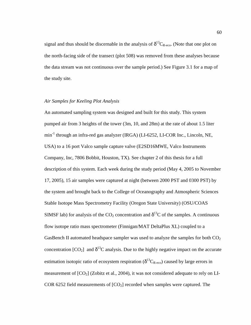
60 signal and thus should be discernable in the analysis of δ13CR-eco. (Note that one plot on
the north-facing side of the transect (plot 508) was removed from these analyses because
the data stream was not continuous over the sample period.) See Figure 3.1 for a map of
the study site.
Air Samples for Keeling Plot Analysis
An automated sampling system was designed and built for this study. This system
pumped air from 3 heights of the tower (3m, 10, and 28m) at the rate of about 1.5 liter
min-1 through an infra-red gas analyzer (IRGA) (LI-6252, LI-COR Inc., Lincoln, NE,
USA) to a 16 port Valco sample capture valve (E2SD16MWE, Valco Instruments
Company, Inc, 7806 Bobbit, Houston, TX). See chapter 2 of this thesis for a full
description of this system. Each week during the study period (May 4, 2005 to November
17, 2005), 15 air samples were captured at night (between 2000 PST and 0300 PST) by
the system and brought back to the College of Oceanography and Atmospheric Sciences
Stable Isotope Mass Spectrometry Facility (Oregon State University) (OSU/COAS
SIMSF lab) for analysis of the CO2 concentration and δ13C of the samples. A continuous
flow isotope ratio mass spectrometer (Finnigan/MAT DeltaPlus XL) coupled to a
GasBench II automated headspace sampler was used to analyze the samples for both CO2
concentration [CO2] and δ13C analysis. Due to the highly negative impact on the accurate
estimation isotopic ratio of ecosystem respiration (δ13CR-eco) caused by large errors in
measurement of [CO2] (Zobitz et al., 2004), it was not considered adequate to rely on LI-
COR 6252 field measurements of [CO2] recorded when samples were captured. The

61 OSU/COAS SIMSF lab came up with a unique solution to increase the accuracy of
measurement of [CO2] by using the integral of the mass spectrometer voltage output
versus time signal to determine [CO2].
Keeling Plot Analysis
The value of δ13CR-eco was determined from each set of weekly air samples using
a two end-member mixing model, or Keeling plot (Keeling 1958, 1961, Buchmann and
Ehleringer 1998, Flanagan and Ehleringer 1998). The Keeling method requires plotting
the δ13C value for each sample against the inverse of its CO2 concentration on a graph.
The y-axis intercept of a geometric mean regression for all air samples of a particular
sample period is the estimation of δ13CR-eco for that dataset. The geometric mean
regression technique has been chosen over ordinary least squares regression because it is
considered more accurate for cases in which there are errors in both the x and y variables
(Pataki et al. 2003). The standard errors of δ13CR-eco measurements were estimated using
the bootstrapping method (Chernick 1999) of standard error determination. Bootstrapping
is a technique which uses the original data from a set to build a large number of datasets
(in this case, 5000) by randomly re-sampling the original dataset. The Keeling plot
technique was then applied to each of these re-sampled datasets and a distribution of
intercepts was determined. The standard error of this distribution was then chosen as the
error bounds for that particular dataset’s intercept. These errors were then minimized by
successively applying a jackknife algorithm (Chernik 1999), which identifies and
removes the data point which has the most negative effect on the resulting standard error

62 and then recalculating the standard error based on the new dataset. Using the jackknife
technique, potential outliers were identified. These potential outliers were then subjected
to a set of criteria to determine whether or not they should be eliminated from the dataset.
The final datasets were constrained to have a minimum value of CO2 range and minimum
number of regression data points (20ppm and 8 data points, respectively) to make certain
that the results retained statistical significance (Pataki et al. 2003).
Vapor Pressure Deficit
The seasonal values of δ13CR-eco were compared to the vapor pressure deficit
(VPD) of the canopy air to determine if a correlation existed between these two variables.
VPD was calculated from air temperature measurements at 15 minute intervals using a
curve fitted to predict saturation vapor pressure from air temperature and then
multiplying the result by the value (1-Rh) (where Rh is the relative humidity of the
canopy air). Air temperature and relative humidity data for the canopy air were measured
using shielded probes (HMP45C, Vaisala, Helsinki, Finland) at the tower and at each of
the eight transect plots. Maximum and daily average VPD were determined from these 15
minute VPD compilations.
Soil Volumetric Water Content
Continuous soil moisture measurements were made at three depths (5cm, 30cm
and 100cm) at each of four locations in each of the eight transect sites using ECH20 soil
moisture probes (EC-10, Decagon Devices, Pullman WA). These instruments were

63 placed in service at different times during the sampling season, resulting in gaps in soil
moisture data for some plots. The data from these probes were stored as 15 minute
averages on a datalogger (CR 10x, Campbell Scientific Inc.). Some individual sensors
malfunctioned over the course of the sampling period and their data was removed from
the dataset. After the datasets were cleaned of the data from malfunctioning sensors, daily
average values for all depths were determined.
VPD and Soil Volumetric Water Content to Keeling Intercept Correlation Statistics
Relationships between seasonal δ13CR-eco patterns with both VPD and soil
volumetric water content were estimated using Pearson’s product-moment correlation
(Barbour et al. 2005, Bowling et al. 2002). The potential for temporal lag was also
explored (Bowling et al. 2002). The lag analysis was performed by offsetting the daily
averages of the independent variable (VPD or soil volumetric water content) to the
dependent variable (seasonal δ13CR-eco pattern) for the target number of days (between 0
days and 10 days for these analyses). For these analyses, it was assumed that the
dependent variable response would lag the independent variable change, so the offset
days all preceded the dependent variable patterns. The significance of the correlations
was determined using the method described by Helsel and Hirsch (1992). The Helsel and
Hirsch method of determining correlation significance compares the calculated value tr to
the corresponding value of t from a student’s t-test for the desired level of confidence in
the outcome (in this case, 95%) and the number of degrees of freedom using the equation:
tr = (r*(n-2)0.5)/((1-r2)0.5)

64
where r is the Pearson’s correlation coefficient and n is the number of data points
in the data set. This equation is then solved for the critical value of the Pearson’s
correlation coefficient which yields a tr equal to the desired t from the student’s t-test.
Values of r exceeding this critical value (or lower than the critical value, if the correlation
is negative) are considered significant.
Results: Carbon Isotopic Composition of CO2
The values of δ13CR-eco over the sampling period of this study ranged from -
26.83 to -22.960/00 (Figure 3.3), with standard errors ranging from 0.27 to 1.830/00. A
typical Keeling plot for one of the sample days (Figure 3.2) shows a high degree of
correlation (r2 = 0.997) between the δ13C values of the air and the inverse of the
associated CO2 measurements. The pattern of the isotopic composition of CO2 (Figure
3.3) shows a relatively flat response to the dry summer months, rising later in the season
when significant precipitation was recorded. Attempts to capture air samples earlier in
2005 (May and June) were unsuccessful because of automated sampling system failure.
After these collections were made, a closer investigation of the data revealed that samples
collected during the early evening were not representative of the watershed because the
canopy air did not become well-mixed until later in the evening. Therefore, individual
data points for these early-evening samples were removed from the datasets before the
Keeling analyses were conducted.

65 Correlations between VPD and δ13CR-eco
VPD was calculated from temperature and relative humidity data taken at all plots
along the transect (Figure 3.1) as well as at a height of 10m on the tower. Minimum and
maximum values of 15-min averages of VPD were 5.0 and 1672 Pa for the plot averages,
while the corresponding values for the tower were 2.7 and 1758 Pa. Patterns of VPD for
all plots were well correlated (Pearson correlation ranged from 0.98 to 1.0) with one
another, indicating that the average VPD of all plots accurately represented the variation
in VPD for the entire transect (Figure 3.4). A correlation of this average plot VPD with
that of the VPD measured at the tower also yields a high correlation (Pearson correlation
= 0.99), indicating that tower VPD can be used as accurate proxy for the VPD of the
transect (Figure 3.5). For simplicity in analysis, and justified by the high degree of
correlation between plots and plot average and Tower, only the Tower VPD values were
used to correlate to Keeling intercepts. This correlation of Keeling intercepts to Tower
VPD for 0 to 10 day lags yielded Pearson correlation coefficients between -0.49 and 0.11,
which were not significantly different from 0 using the Helsel and Hirsch significance
criteria (r = ± 0.58) (Figure 3.6).
Soil Volumetric Water Content Correlation
Average soil volumetric water content from the 30cm depth ranged from 7.2 % at
plot 507 on September 12, 2005, to 44.3% at plot 501 on November 15, 2005. The 30cm
depth was chosen for correlation to Keeling intercepts due to its dominance as the source
of water for forests composed of predominantly Douglas-fir (Brooks et al. 2006). A

66 comparison of plots by elevation showed a high correlation between soil volumetric
water content for upslope versus downslope plots (r = 0.90), with the higher elevation
plots (upslope) having an average of 6.3 ± 1.2 % (1 s.d.) higher soil volume than that of
the lower elevation (downslope) plots (Figure 3.7). A comparison of plots grouped by sun
exposure did not show a strong soil volumetric water content correlation (r = 0.58)
(Figure 3.8) , with south-facing plots having an average of 7.8 ± 3.7 % (1 s.d.) higher soil
volumetric water content than that of the north-facing plots. Both of these groupings
showed a strong correlation, with virtually no lag, to significant rainfall events (greater
than approximately 4mm, Pypker et al. 2005).
Soil volumetric water content on plots grouped by elevation was not significantly
correlated to Keeling intercepts (Helsel and Hirsch,1992). The values of correlation
ranged from -0.09 to -0.46 for upslope plots and -0.15 to -0.47 for downslope plots
(Figure 3.9). Soil volumetric water content on plots grouped by sun exposure showed a
significant correlation between Keeling intercepts and south-facing plot soil moisture
ranging from -0.77 to -0.69, but there was no significant correlation for north-facing plots
(r = -0.08 to 0.29). It was expected that the isotopic signature of the ecosystem
respiration would lag behind the soil moisture changes, but the data showed no
significant lag response (Figure 3.10). The lagged response of ecosystem respiration is
thought to be a consequence of the fact that about 70% of ecosystem respiration comes
from soil microbial respiration (Eckblad and Hogberg, 2001). The sugars which supply
fuel for these microbes are supplied by vegetation via phloem transport. There is a delay
between when the sugars are fixed in the leaves and when they are liberated from the soil

67 and become part of the ecosystem respiration signal because of: (1) the phloem transport
time; (2) the time it takes sugars to diffuse into the soil and reach the microbes; (3) the
time it takes for the microbes to digest and respire these sugars; and (4) the time it takes
the respiration to diffuse from the microbial source to the soil surface. All of these delay
times add in sequence to produce a lag between the soil moisture signal which produces
the change in isotopic composition of the sugars produced by assimilation due to stomatal
modulation and the time it takes this signal to reach the ecosystem as soil respiration.
Discussion:
The seasonal pattern of isotopic composition of ecosystem respiration observed in
this study is consistent with the patterns observed in other studies for forests of similar
vegetative compositions and climates (Bowling et al. 2002, Fessenden and Ehleringer
2003). During the initial stages of the growing season, while the soils of the forest are
still relatively moist, vegetation has adequate access to water. Accordingly, the vegetation
will respond by maintaining high levels of stomatal conductance to increase their rate of
carbon uptake. The ratio of carbon dioxide concentration in the leaf interior to that of the
atmosphere (ci/ca) remains relatively high in this situation, which promotes
discrimination against the heavier isotope of carbon (Farquhar et al. 1989). As the
summer progresses and precipitation drops, soils begin to dry out, limiting vegetation’s
access to water. In order to avoid cavitation and the associated damage to xylem cells,
trees begin to close their stomata, lowering stomatal conductance. This drop in
conductance decreases the ci/ca ratio, which reduces discrimination against the heavier

68 carbon isotope. As a result of this mechanism, as the season progresses and access to
moisture is reduced, the newly-fixed sugars should show an increase in the ratio of 13C to
12C. Recent studies have shown that a large amount of recently-fixed carbon may cycle
quickly through an ecosystem (Eckblad and Hogberg, 2001), with the result that the
isotopic composition of respired CO2 may be heavily influenced by recently-fixed sugars.
Thus, the pattern of change in isotopic composition of recently fixed sugars is visible in
the respiration signal, as observed in this study. In the early part of the summer, values of
δ13CR-eco were relatively depleted. As the soils began to dry out, δ13CR-eco became
enriched.
If the only component of ecosystem respiration were to come directly from the
use by vegetation of recently fixed sugars, the respiration isotopic composition signal
could be used as a direct proxy for the state of vegetative drought stress. However,
respiration from soils and vegetation may be fueled by stored carbon, such as starches or
other complex biochemicals, as well as newly-fixed carbon, and this mixed source may
confound the signal (Mortazavi et al. 2002, Buchman 1997). In soils, the partitioning of
respiration between heterotrophic and autotrophic components is a topic of intense study
(Chambers et al. 2004, Rochette et al. 1999, Bhupinderpal et al. 2003) and is a topic of
interest in the overall HJ Andrews Airshed project. The partitioning of respiration signals
is beyond the scope of this thesis, however.
Many studies have been aimed at connecting the seasonal pattern of Keeling
intercepts with drought stress variables such as VPD (Bowling et al. 2002, Sanford et al.
1986, Condon et al. 1992), soil volumetric water content (Fessenden et al. 2002) and

69 precipitation (Ometto et al. 2002, Pataki et al. 2003, Bowling et al. 2002). The results of
this study indicate that VPD was not significantly correlated with seasonal Keeling
intercepts, unlike results from many previous studies (Bowling et al. 2002). The
correlations between soil volumetric water content of south-facing plots and seasonal
Keeling intercepts were strong, but there were no significant correlations between the
isotopic values and soil volumetric water content of north-facing slopes. When soil
volumetric water content was grouped by elevation, no significant correlations were
found. Past research has found lags of between one and four days between VPD and δ13C
of CO2 respired by roots (Eckblad and Hogberg 2001) and five to ten days between VPD
and ecosystem respiration (Bowling et al. 2002), yet the data from this study do not show
significant lags between either VPD or soil volumetric water content and seasonal
Keeling plot intercepts.
The lack of correlation between VPD and seasonal Keeling intercepts may lie in
the timing of the sampling period. Although attempts were made to procure air samples
for respiration analysis in May and June of 2005, these data points were rejected due
either to equipment malfunction or lack of sufficient CO2 range. The physiological
connection between soil volumetric water content and VPD with respect to isotope
discrimination is rooted in how those variables affect stomatal function. During the early
part of the growing season, soil volumetric water content is relatively high, so that
vegetation’s access to a pool of water for transpiration is plentiful. During this period of
time, isotopic discrimination will be dictated by the rise and fall of VPD. As the growing
season progresses and soil moisture begins to decline due to the cumulative effects of
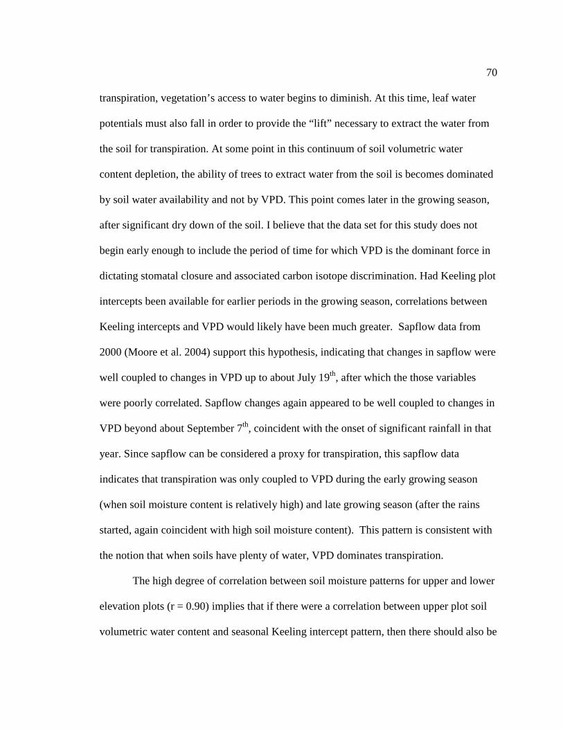
70 transpiration, vegetation’s access to water begins to diminish. At this time, leaf water
potentials must also fall in order to provide the “lift” necessary to extract the water from
the soil for transpiration. At some point in this continuum of soil volumetric water
content depletion, the ability of trees to extract water from the soil is becomes dominated
by soil water availability and not by VPD. This point comes later in the growing season,
after significant dry down of the soil. I believe that the data set for this study does not
begin early enough to include the period of time for which VPD is the dominant force in
dictating stomatal closure and associated carbon isotope discrimination. Had Keeling plot
intercepts been available for earlier periods in the growing season, correlations between
Keeling intercepts and VPD would likely have been much greater. Sapflow data from
2000 (Moore et al. 2004) support this hypothesis, indicating that changes in sapflow were
well coupled to changes in VPD up to about July 19th, after which the those variables
were poorly correlated. Sapflow changes again appeared to be well coupled to changes in
VPD beyond about September 7th, coincident with the onset of significant rainfall in that
year. Since sapflow can be considered a proxy for transpiration, this sapflow data
indicates that transpiration was only coupled to VPD during the early growing season
(when soil moisture content is relatively high) and late growing season (after the rains
started, again coincident with high soil moisture content). This pattern is consistent with
the notion that when soils have plenty of water, VPD dominates transpiration.
The high degree of correlation between soil moisture patterns for upper and lower
elevation plots (r = 0.90) implies that if there were a correlation between upper plot soil
volumetric water content and seasonal Keeling intercept pattern, then there should also be

71 a correlation between the lower plot soil volumetric water content and the seasonal
Keeling intercept pattern. The reverse is also true: if the lower elevations did not show a
correlation, then neither should the upper elevations. This was indeed the case- no
significant correlation was found for either upper or lower elevation plots and seasonal
Keeling intercepts. It is worth noting that grouping all soil moisture plots together for the
entire transect also produces no significant correlation with seasonal Keeling intercepts.
Indeed, the pattern of correlation over time lag was quite similar for upper elevation,
lower elevation, and all plots combined.
The correlation Keeling intercepts and the soil water content of south-facing plots
was significant, whereas the correlation for north-facing plots was not. It has been shown
by Pypker et al. (2006) that the nighttime air drainage from which these samples were
taken is well mixed, so stratification or preferential sampling of one side of the watershed
is not likely, yet the ecosystem respiration signal appears to be correlated with the south-
facing slope soil volumetric water content. I propose three hypotheses to explain this
finding. The first hypothesis pertains to airflow patterns. It is possible that air may enter
the watershed predominantly from the south face, flooding the basin with air from the
south side. If this were the case, then the ecosystem respiration signal from the north-
facing slope may not be making it down to the site of the tower and thus was not
represented in the air sampling conducted at the base of the watershed. However, this
hypothesis is not considered likely. The theory behind cold air drainage is that cooling at
the ground level causes surface air to increase in density, which then flows downhill due
to gravity, where it collects in the bottom of the watershed. Continued cooling of the

72 slopes above this pool of air in the bottom of the watershed causes further cold air
drainage off of the slope, pushing the collected air in the bottom out of the base of
watershed. The tower at the base of the watershed lies in this drainage path. Since the
flow of air is turbulent (Pypker et al. in press), the air in this drainage is well mixed. The
north slope of the watershed is shaded earlier in the day than the south-facing slope and
therefore should begin draining earlier. If there were to be an uneven representation of
one slope’s respiration signal over the other, this geographic layout should favor the north
slope, not the south slope.
The second hypothesis is that the volumetric water content of the south-facing
slope represents the overall state of the entire watershed better than that of the north-
facing slope. If this were true, then the respiration contributions of both slopes of the
watershed could be represented in the dataset, yet the correlation between δ13CR-eco and
north-facing slope soil moisture would be poor. Essentially, the soil volumetric water
content of the thin line of the transect is being used as a proxy for the entire surface area
of the watershed (or at least of the portion of the watershed contributing respiration to the
drainage, also termed the “footprint” of the watershed). It is impossible to say, given
current the dataset, whether or not the conditions of the plots on the south-facing slope
better represent the entire watershed “footprint” than the plots on the north-facing slope.
To test this hypothesis, a sampling of multiple locations in the watershed would need to
be compared to corresponding transect data to see determine what best represents the
entire watershed’s soil moisture signal. Such an endeavor is beyond the scope of this
paper.

73
The third hypothesis is that the north-facing slope of the watershed had
significantly lower respiration rates than the south-facing side due to greater moisture
stress (Zavitkowski et al. 1968; Burton et al. 1998). As a result of this reduction in
respiration rate, the north-facing slope would contribute less to the total amount of
respired CO2 captured in the samples collected at the tower. The patterns for soil
volumetric water content for the north-facing slope versus the south-facing slope lend
support to this argument. During the early part of the sampling period, the north-facing
slope soil moisture values were consistently nearly 12% lower than those of the south-
facing slope. Average soil depth (measured to the bottom of the B horizon) on the south-
facing slope was about 105cm, whereas the equivalent measurement for the north slope is
81cm (Padilla, private communication). Assuming that both slopes started the year with
similar water content (on a percentage basis), the larger volume of soil on the south-
facing slope would provide a larger pool of water for the vegetation on that slope to draw
from, compared to the north side with less soil volume. Assuming the vegetation on both
slopes would begin the growing season with ample soil water available and assuming
roughly equal distributions and size classes of vegetation, the slope with the smaller pool
of water available should reach drought stress conditions ahead of the slope with the
larger pool. The smaller soil volume of the north-facing slope and the lower soil
volumetric water content of that slope at the beginning of the sampling season lend
support to this hypothesis. Unfortunately, data for the early part of the growing season
(May and June 2005) was not available for this study. It may have been possible to
extract the data necessary to confirm this hypothesis by looking for declining values of

74 CO2 concentration as drought stress on the north-facing slope developed. As the north-
facing slope was heading into drought stress during this timeframe, the isotopic
composition of the north-facing slope air drainage would have reflected this transition.
Had this early data been available, this signal should have also been detectable, which
may have provided confirming evidence of this hypothesis. Streamflow data for WS-1
from the period 1997-2002 (Jones and Post, 2004) lend support to this hypothesis:
continuously declining streamflow starting in May and continuing until September
indicate that the watershed was drying out during this period. The loss of stream flow in
the dry months would be indicative of a general decline in soil moisture content, which
supports the hypothesis that respiration declined on the north-facing slope due to loss of
soil moisture and associated drought stress.
Other data that lend more direct support to the third hypothesis. For the current
year the value of foliar respiration for the south-facing plots averaged -7.8 µmolm-2s-1
whereas for the north-facing plots the corresponding value was -4.3 µmolm-2s-1 (Bond,
private communication) (figure 3.11). Soil respiration values for south-facing and north-
facing were -7.0 and -3.0 µmolm-2s-1, respectively (Kayler, private communication)
(figure 3.11). With respect to both foliar and soil respiration, the south-facing slope
respired at nearly twice the rate of the north-facing slope, again reinforcing the notion
that the respiration signal seen at the base of the watershed during the sample period was
dominated by respiration from the south-facing slopes.
Why would soil accumulation be lower in the north-facing slope? South-facing
slopes generally dry out earlier in the year than north-facing slopes, limiting vegetative

75 carbon assimilation and detritus production. As a general rule, this should favor soil
development and vegetation growth for north-facing slopes. However, differences in the
topography of individual sites may alter the outcome of these generalized mechanisms.
The average incline of the north-facing slope at the study site is about 93% whereas that
of the south slope is about 65% (Padilla, private communication). It is possible that this
difference in slope creates soil instability on the north-facing slopes, promoting slides and
soil movement towards the base of the watershed and is thus responsible for the north-
facing slope having less soil volume than the south-facing slope. There is a great deal of
blowdown and apparent soil instability on the north-facing slope, which also supports this
position.
Conclusions:
The pattern of isotopic composition of ecosystem respiration at WS-1 of the HJ
Andrews Experimental Forest from July to September 2005 is consistent with
expectations of a forest in the midst of drought stress. Contrary to results of many other
researchers, the seasonal Keeling intercept pattern did not correlate significantly to the
pattern of VPD during the sample period, but did correlate significantly to the patterns of
soil volumetric water content on the south-facing slope of the watershed. The lack of
correlation with VPD is likely due to the fact that the sampling period did not include the
early part of the growing season, where soil moisture is plentiful and VPD dominates
stomatal modulation. The correlation of Keeling intercept pattern with south-facing soil
moisture is likely due to the fact that soil volumetric water content on that face was

76 sufficient to allow the vegetation to continue to assimilate carbon and maintain higher
respiration rates in the later part of the season.
Acknowledgements and Credits:
Tom Pypker was immensely helpful in all aspects of this project, from design and
construction of the automated sampler to data acquisition and manuscript editing. This
project literally could not have been completed without his help. Advice and coaching on
field work techniques and assistance in data acquisition from Zach Kayler, Holly
Barnard, Claire Phillips, Julian Licata and Dave Conklin were greatly appreciated. Zac
Kayler, Aidan Padilla, and Barb Bond provided data to support hypotheses on soil depth.
My advisers Barb Bond, Elizabeth Sulzman, and Julia Jones provided education,
encouragement, and advice at critical junctures and were of great aid in the production of
this thesis.

77
Figure 3.1: HJ Andrews Watershed 1 Topographic Map
Topographic map of Watershed 1 at HJ Andrews Experimental Forest. The 37m tower at the base of the watershed and the 8 plots which make up the transect serve as the data collection points for the isotopic composition of ecosystem respiration, VPD, and soil moisture used as variables in this study. The 21.3m ridge tower has been used in subsequent studies to determine values of wind speed, wind direction, and isotopic composition of the air above the canopy.
37m tower
Transect- 4 plots per side 21.3m ridge
tower

78
Figure 3.2: Typical Keeling Plot
Keeling Plot of Airshed Tower DataAugust 10, 2005
1/[CO2]
0.00230 0.00235 0.00240 0.00245 0.00250 0.00255 0.00260 0.00265
δ13C
-10.5
-10.0
-9.5
-9.0
-8.5
-8.0
-7.5
Geometric Mean Regression Resultsδ13Ceco = -26.35 + 7069.13* [1/CO2], r
2= 0.9969
Typical Keeling plot for HJ Andrews Airshed project. This data is from August 10, 2005. Geometric mean regression analysis of the data for this date resulted in an intercept of -26.35 0/00.

79
Figure 3.3: Seasonal graph of Keeling intercepts
Keeling plot intercept graph for 2005 data from WS-1 of HJ Andrews Experimental Forest. DOY’s 315 and 236 were removed from the dataset because the air sample data was collected before the airshed drainage became well mixed. DOY 249 was removed because the data was corrupted by a malfunction of the collection storage valve. DOY 315 was removed because the CO2 range was too small to support a statistically valid intercept. The first trap sample was removed from each dataset because the sample timing was premature. For the 2005 growing season, the intercepts ranged between -26.83 and -22.960/00. Error bars represent +/- 1 standard error.
2005 Keeling Intercepts with Standard Error Bars
DOY
180 200 220 240 260 280 300
Kee
ling
Inte
rcep
ts, δ
13C
r-ec
o, p
erm
il
-30
-28
-26
-24
-22
-20

80
Figure 3.4: Seasonal values of VPD for all plots on transect
2005 VPDs for individual plots across transect in WS-1 of HJ Andrews Experimental Forest. Data for temperature and relative humidity at each plot were used to determine VPD. Note that the pattern for each plot is virtually identical, indicating that for the purposes of establishing correlations with isotopic composition of ecosystem respiration, any one plot could be used in place of the others without a change in the correlation statistics (Pearson correlation ranged from 0.98 to 1.0).
H J A n d r e w s 2 0 0 5 W S - 1 In d iv id u a l P lo t V a p o r P r e s s u re D e f ic i t
D a y o f Y e a r
2 2 0 2 4 0 2 6 0 2 8 0 3 0 0
VP
D, P
a
0
5 0 0
1 0 0 0
1 5 0 0
2 0 0 0
P lo t 5 0 1 P lo t 5 0 2 P lo t 5 0 4 P lo t 5 0 7 P lo t 5 0 8 P lo t 5 1 0 P lo t 5 1 2

81
Figure 3.5: Comparison of Tower VPD to Plot Average VPD
Comparison of VPD of tower with average of VPD of transect plots. The patterns are obviously highly correlated (Pearson’s correlation coefficient = 0.99)
H J Andrew s 2005 W S-1 VPD C om parison: Tower to P lo t Average
D ay of Year
180 200 220 240 260 280 300
VP
D, P
a
0
200
400
600
800
1000
1200
1400
1600
1800
2000
Tow er P lo t average

82
Figure 3.6: Keeling Intercepts correlated to Tower VPD
Growing season Keeling intercepts correlated to Tower VPD with temporal lag. The Pearson’s correlation coefficient for Keeling intercept was correlated to the corresponding values of Tower VPD, starting with a lag of 0 days and ending with a 10 day lag (Keeling intercept lag behind VPD, assuming that the isotopic response of the ecosystem respiration lagged behind the VPD which may have been responsible for the isotopic changes in respiration). Note that there are no values of the Pearson’s correlation coefficient which are significant after applying Helsel and Hirsch’s significance test.
K e e l in g I n te r c e p t s c o r r e la te d to v a p o r p r e s s u r e d e f ic i t
L a g , d a y s
0 2 4 6 8 1 0
Pea
rson
Cor
rela
tion
Coe
ffici
ent ,
r
- 0 .6
- 0 .4
- 0 .2
0 .0
0 .2
0 .4
0 .6
c o r r e la t io n s ig n i f ic a n c e = 0 .5 8 2 , w it h n = 9 , 9 5 % c o n f id e n c e
c o r r e la t io n s ig n i f ic a n c e = - 0 . 5 8 2 ,n = 9 , 9 5 % c o n f id e n c e

83
Figure 3.7: Comparison of Soil Moisture on upslope plots versus downslope plots
Comparison of soil moisture at plots on grouped by slope position. Soil moisture patterns for upslope and downslope plots show high degree of correlation with each other (Pearson correlation =0.90). Note response of soil moisture to larger precipitation inputs is immediate, whereas for small values of precipitation, no effect on soil moisture is obvious. This is probably due to the fact that the canopy did not saturate in the smaller precipitation events, thus effectively no rainfall reached the soil.
HJ Andrews 2005 WS-1 Soil Moisture: Plot Elevation Comparison
Day of Year
200 220 240 260 280
Soi
l Moi
stur
e, %
or Pre
cipi
tatio
n, m
m
0
10
20
30
40
Kee
ling
Inte
rcep
t, δ1
3 C, p
erm
il-28
-27
-26
-25
-24
-23
Upslope (Plots 501, 502, 510, 512)Downslope (Plots 504, 505, 507)PrecipitaionKeeling Intercepts

84 Figure 3.8: Comparison of Soil Moisture on north-facing to south-facing
plots
Comparison of soil moisture at plots on grouped by slope directional orientation. Soil moisture patterns for south-facing and north-facing plots show low degree of correlation with each other (Pearson correlation =0.58). Again, the same pattern of soil moisture changes with magnitude of precipitation events is seen.
HJ Andrews 2005 WS-1 Soil Moisture: Plot Direction Comparison
Day of Year
200 220 240 260 280
Soi
l Moi
stur
e, %
or
Pre
cipi
tatio
n, m
m
0
10
20
30
40
Kee
ling
Inte
rcep
ts, δ
13C
, per
mil
-28
-27
-26
-25
-24
-23
South facing averageNorth facing averagePrecipitationAverage of all PlotsKeeling Intercepts

85
Figure 3.9: Keeling intercept correlations to soil moisture for upslope and downslope plots
Keeling intercept correlated to soil moisture grouped by elevation. Note that there are no significant correlations for either upslope grouped plots or downslope grouped plots after applying the Helsel and Hirsch significance test.
Soil m oiture to Kee ling in tercept corre la tion (grouped by e levation)
Lag, days
0 2 4 6 8 10
Pea
rson
Cor
rela
tion
Coe
ffici
ent,
r
-0 .60
-0.40
-0.20
0.00
0.20
0.40
0.60
U pslope (P lo ts 501, 502, 510, 512)D ow nslope (P lo ts 504, 505, 507)
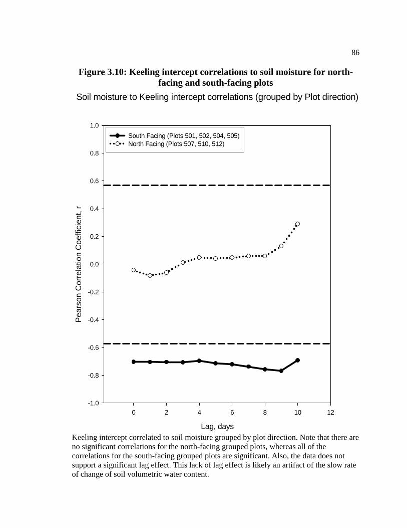
86
Figure 3.10: Keeling intercept correlations to soil moisture for north-facing and south-facing plots
Keeling intercept correlated to soil moisture grouped by plot direction. Note that there are no significant correlations for the north-facing grouped plots, whereas all of the correlations for the south-facing grouped plots are significant. Also, the data does not support a significant lag effect. This lack of lag effect is likely an artifact of the slow rate of change of soil volumetric water content.
Soil moisture to Keeling intercept correlations (grouped by Plot direction)
Lag, days
0 2 4 6 8 10 12
Pea
rson
Cor
rela
tion
Coe
ffici
ent,
r
-1.0
-0.8
-0.6
-0.4
-0.2
0.0
0.2
0.4
0.6
0.8
1.0
South Facing (Plots 501, 502, 504, 505)North Facing (Plots 507, 510, 512)

87
Figure 3.11: Table of soil depth and ecosystem respiration
Measurement
South Facing
North Facing
Soil Depth to bottom
of B Horizon
105cm
81cm
Foliar Respiration
-7.8 mmolm-2s-1
-4.2 mmolm-2s-1
Soil Respiration
-7.0 mmolm-2s-1
-3.0 mmolm-2s-1
Table of soil depth and ecosystem respiration values. These data were supplied by other members of the HJ Andrews Airshed Project team. The foliar respiration values are averages of 2006 measurements while the soil respiration measurements are averages of combined 2005 and 2006 values. The soils depth measurements were averaged from measurements made in 2005 from 4 soil pits dug at 2 sites per slope.

88 References: Baldocchi, D. 1997. Measuring and modeling carbon dioxide and water vapour exchange over a temperate broad-leaved forest during the 1995 summer drought. Plant, Cell and Environment 20:1108-1122. Baldocchi, D. 2003, Assessing the eddy covariance technique for evaluating carbon dioxide exchange rates of ecosystems: past, present, and future, Global Change Biology, Vol 9, Page 479 Barbour, M.M., Hunt, J.E, Dungan, R. J., Turnbull, M.H., Brailsford, G.W., Farquhar, G.D., Whitehead, D., Variation in the degree of coupling between d13C of phloem sap and ecosystem respiration in two mature Nothofagus forests, New Phytologist, Volume 166, Page 497, May 2005. Bhupinderpal-Singh, Nordgren A, Ottosson Lofvenius M, Hogberg MN, Mellander P-E, Hogberg P, 2003. Tree root and soil heterotrophic respiration as revealed by girdling of boreal Scots pine forest: extending observations beyond the first year, Plant, Cell, Environ., 26, 1287-1296 Black, T. A., G. d. Hartog, H. H. Neumann, P. D. Blanken, P. C. Yang, C. Russell, Z. Nesic, X. Lee, S. G. Chen, R. Staebler, and M. D. Novak. 1996. Annual cycles of water vapour and carbon dioxide fluxes in and above a boreal aspen forest. Global Change Biology 2:219-229. Bowling, D.R., McDowell, N.G., Bond, B.J., Law, B.E., Ehleringer, J.R., 13C content of ecosystem respiration is linked to precipitation and VPD, Oecologia (2002), 131:113-124. Brooks, J.R., Meinzer, F.C., Warren, J.M., Domec, J.C., Coulombe, R., 2006, Hydraulic redistribution in a Douglas-fir forest: lessons from system manipulations, Plant, Cell and Environment, (2006) 138-150 Bowling, D.R., Tans, P.P., Monson, R.K., 2001, Partitioning net ecosystem carbon exchange with isotopic fluxes of CO2, Global Change Biology, Vol 7, Page 127 Buchman, N., and J. A. Ehleringer. 1998, CO2 concentration profiles, and carbon and oxygen isotopes in C3 and C4 crop canopies, Agricultural and Forest Meteorology 89:45-58. Buchman, N, Kao, W, Ehleringer, J, 1997, Influence of stand structure on Carbon 13 of vegetation, soils and canopy air within deciduous and evergreen forests in Utah, United States, Oecologia, Vol 10, number 1

89 Burton, A.J., Pregitzer, K.S., Zogg, G.P., Zak, D.R., 1998, Drought reduces root respiration in sugar maple forests, Ecological Applications, Vol. 8, No.3 Condon, A.G., Richards, R.A., Farquhar, G.D., 1992,The effect of variation in soil water availability, vapour pressure deficit and nitrogen nutrition on carbon isotope discrimination in wheat, Australian Journal of Agricultural Research 43(5) 935 - 947 Chambers, J.Q., Tribuzy, E.S., Toledo, L.C., Crispm, BF,Higuchi, N., Dos Santos, J., Arau’jo, A.C., Kruijt, B., Nobre, A.D., trumbore, S.E., 2004, Respiration from a tropical forest ecosystem: Partitioning of sources and low carbon use efficiency, Ecological Applications, 14(4) Supplement 2004, 72-88 Chernick, M.R., Bootstrap methods: a practitioner’s guide, 1999, John Wiley & Sons. Ehleringer, J. R., A. E. Hall, and G. D. Farquhar. 1992. Stable isotopes and plant carbon- water relations. Academic Press, San Diego, CA. Eckblad A, Högberg P. 2001. Natural abundance of 13C in CO2 respired from forest soils reveals speed of link between tree photosynthesis and root respiration, Oecologia 127: 305-308 Farquhar, GD, Ehleringer, JR, Hubick, KT, 1989. Carbon isotope discrimination and photosynthesis. Annu. Rev. Physiol. Plant Mol. Biol., 40, 503-537 Flanagan, L. B., and J. A. Ehleringer. 1998. Ecosystem - atmosphere CO2 exchange: interpreting signals of change using stable isotope ratios, Trends in Ecology and Evolution 13:10-14. Fessenden, JE, Ehleringer, JR, 2003, Temporal variation in d13C of ecosystem respiration in the Pacific Northwest: links to moisture stress, Oecologia 136:129-136 Fleagle, R. G. 1950. A theory of air drainage. Journal of Meteorology 7:227-232. Gifford, R.M., 1994,The Global Carbon Cycle: a Viewpoint on the Missing Sink, Australian Journal of Plant Physiology 21(1) 1 – 15 Harmon, M. E., K. Bible, M. G. Ryan, D. C. Shaw, H. Chen, J. Klopatek, and X. Li. 2004. Production, respiration, and overall carbon balance in an old-growth Pseudotsuga-Tsuga forest ecosystem. Ecosystems 7:498-512. Helsel, D.R., and R.M. Hirsch, Statistical Methods in Water Resources, Elsevier, Science Publishers, Amsterdam, The Netherlands, 1992.

90 Jones, J.A. and Post, D.A., 2004, Seasonal and successional streamflow response to forest cutting and regrowth in the northwest and eastern United States, Water Resources Research, Vol. 40, W05203 Keeling, C. D. 1958. The concentration and isotopic abundances of atmospheric carbon dioxide in rural areas, Geochimica et Cosmochimica Acta 13:322-334. Manins, P. C., and B. L. Sawford. 1979. Katabatic winds: A field study. Quarterly Journal of the Meteorological Society 105:1011-1025. Martin, M.E., Aber, J.D., 1997, High Spectral Resolution Remote Sensing of Forest Canopy Lignin, Nitrogen, and Ecosystem Processes, Ecological Applications, Vol. 7, No. 2, pp. 431-443 Monteith, J. L., and M. H. Unsworth. 1990. Principles of Environmental Physics, 2nd edition. Edward Arnold, New York. Moore, G.W., Bond, B.J., Jones, J.A., Phillips, N., Meinzer, F.C., 2004, Structural and compositional controls on transpiration in 40 and 450-year-old riparian forests in western, Oregon, USA, Tree Physiology 24, 481-491 Lavigne, M. B., D. E. Anderson, M. G. Ryan, D. E. Anderson, D. D. Baldocchi, P. M. Crill, D. R. Fitzjarrald, M. L. Goulden, S. T. Gower, J. M. Massheder, J. H. McCaughey, M. Rayment, and R. G. Striegl. 1997. Comparing nocturnal eddy covariance measurements to estimates of ecosystem respiration made by scaling chamber measurements at six coniferous boreal sites. Journal of Geophysical Research 105:28977-28985. Mortazavi, B, Chanton, JP, 2002, Carbon isotopic discrimination and control of nighttime canopy d18C-CO2 in a pine forest in the southeastern United States, Global Biogeochemical Cycles, Vol. 16, No. 1 Ometto, J.P., Flanagan, L.B., Martinelli, L.A., Moreira, M.Z., Ehleringer, J.R., 2002, Carbon isotope discrimination in forest and pasture ecosystems of the Amazon Basin, Brazil, Global Biogeochemical Cycles, Vol.16, No. 4, 1109 Pataki, D. E., J. A. Ehleringer, L. B. Flanagan, D. Yakir, D. R. Bowling, C. Still, N. Buchmann, J. O. Kaplan, and J. A. Berry. 2003, The application and interpretation of Keeling plots in terrestrial carbon cycle research, Global Biogeochemical Cycles 17:1022. Pypker, T.G., Unsworth, M.H., Mix, A.C., Rugh, W., Ocheltree, T., Alstad, K., Bond, B.J., 2006, Using nocturnal cold air drainage flow to monitor ecosystem processes in

91 complex terrain: a pilot study on the carbon isotopic composition and advection of ecosystem respiration, in press (Ecol. Apps) Pypker, TG, Bond, BJ, Unsworth, MH, The role of epiphytes in the interception and evaporation of rainfall in old-growth Douglas-fir forests in the Pacific Northwest, Agricultural and Forest Meteorology 130 (2005) 113-129
Rochette, P., L.B. Flanagan, E.G. Gregorich. 1999. Separating soil respiration into plant and soil components using analyses of the natural abundance of carbon-13. Soil Science Society of America Journal 63: 1207-1213 Sanford A.P., Jarvis, P.F., 1986, Stomatal responses to humidity in selected confiers, Tree Physiol 2:89-103 Schimel, D. S., T. G. F. Kittel, S. W. Running, R. K. Monson, A. A. Turnipseed, and D. E. Anderson. 2002. Carbon sequestration studies in Western US mountains. EOS 83:445-448. Staebler, R. M., and D. R. Fitzjarrald. 2004. Observing subcanopy CO2 advection. Agricultural and Forest Meteorology 122:139-156. Swanson, F. J., and M. E. James. 1975. Geology and geomorphology of the H.J. Andrews Experimental Forest, Western cascades, Oregon. Pacific Northwest Forest and Range Experiment Station, Forest Service, U.S.D.A Research Paper PNW-188:1-14. Whiteman, C. D. 1990. Observations of thermally developed wind systems in mountainous terrain. Pages 5-42 in W. Blumen, editor. Atmospheric processes over complex terrain. American Meteorological Society, Boston. Yakir, D., Sternberg, L., 2000, The use of stabile isotopes to study ecosystem gas exchange, Oecologia,, Vol 123, No. 3 Zavitkowski, J., Ferrell, W.K, 1968, Effect of drought upon rates of photosynthesis, respiration, and transpiration of seedlings of two ecotype of Douglas-fir, Botanical Gazette, Vol. 129, No. 4 (Dec., 1968), pp. 346-350

92
Chapter 4
SUMMARY AND CONCLUSIONS
Warming of the terrestrial biosphere due to the anthropogenic addition of carbon
dioxide to the earth’s atmosphere is becoming a major focus of scientific inquiry.
Predictions of the extent of this warming are hampered by uncertainty in the ability of the
earth’s ecosystems to counteract this effect by sequestering carbon dioxide by increases
in the mass of vegetation. Measurement of the carbon isotopic composition of respired
CO2 (δ13CR-eco) is becoming increasingly important to ecosystem studies because the
information contained in this respiration is a good indicator of ecosystem stress and
productivity. This study was conducted as part of a larger research project aimed at
developing and testing the capacity for measuring δ13CR-eco in a small, steeply-sloped
watershed in western Oregon. The goals of this study were: (1) to develop and test an
automated system for sampling nocturnal air to be analyzed in a laboratory for isotopic
composition; (2) to collect samples of the atmosphere from the nocturnal cold air
drainage of a steeply sloped watershed in the HJ Andrews Experimental Forest and bring
those samples back to a laboratory to be analyzed for CO2 concentration and carbon
isotope composition; and (3) to conduct an initial analysis of the relationship between
δ13CR-eco for the first year of deployment and two environmental forcing factors, soil
moisture and atmospheric VPD.
The automated sampling system designed and built for this project provided
significant advantages over previous methods of sample collection. The design objectives
for this automated system included light weight, portability, reliability, fast dynamic

93 response, unattended operation, and the ability to capture, transport, and store samples
over several days with no loss of data integrity with respect to the critical measurement
values of CO2 concentration and carbon isotopic composition. The system was deployed
in rugged terrain on a weekly basis throughout the 2005 sampling system by a variety of
personnel, demonstrating its light weight and portability. With respect to maximum
sampling rate, the dynamic response testing of the automated sampling system provides
evidence that the system can exceed the performance of systems which use glass flasks to
contain samples and should be able to support rapid sampling in research situations
which demand such capability. For this capability to be fully exploited, some changes to
the control architecture would need to be implemented, but those changes are relatively
minor and could be accomplished without much difficulty. The system reliably operated
throughout the nighttime sampling period without technician intervention. Testing
showed that the system provides for storage of samples in the sample loops for at least
three days without significant change in [CO2] or δ13C. This is a clear advantage for
researchers who endeavor to set up such a system and then allow it to perform its
function without supervision. The automated system consistently outperformed the hand
sampling process it replaced and compared favorably with automated sampling systems
described by other researchers with respect to both accuracy and precision of the datasets
which were produced from the air samples collected. The automated system showed itself
to be reliable throughout the sampling season, as evidenced by the positive results of the
weekly system plumbing integrity tests. In conclusion, the system met all design
objectives and functioned as intended, providing a collection of air samples which were

94 successfully analyzed for carbon isotopic composition and carbon dioxide concentration
in the COAS Mass Spectrometer Laboratory.
Although the system met its design objectives and provided the basis for the
primary dataset for this project, there is room for improvement in this system. The system
would benefit from a further reduction in weight, making the system even more portable
and thus easier to deploy in remote and rugged locations. This could be accomplished by
reducing the size and changing the materials for both the sample valve enclosure and the
control enclosure. The Valco sample collection valve is capable of producing air samples
which accurately reflect the source, but this valve is not particularly well suited to the
harsh environment where it was deployed. This situation could be remedied by either
using a sample collection valve from a different manufacturer or by providing a more
robust enclosure for the current valve. No suitable replacement valve candidates have
been identified and providing a more robust enclosure is not a trivial undertaking due to
the need for accessability of the valve for laboratory analysis. Without design or
hardware changes in this area, the weekly integrity testing should be continued to make
certain the collected samples accurately reflect the source. With the addition of a wireless
interface and transmitter, the system could be made to collect data independently and
report back to the experimenter that the system is ready for retrieval. This feature could
enhance the ability of a research team to take samples in multiple remote locations with
minimal personnel requirements while ensuring data which meets pre-set requirements. A
further system enhancement would be a lightweight, portable power source. This feature
would decouple the sampling site from the requirement that a suitable source of power at

95 the site be available. Recent advances in hydrocarbon fuel cell technology may make this
enhancement possible in the near future.
The weekly data stream from this automated system was analyzed for carbon
isotope ratio and CO2 concentration be between May and November 2005. These data
were used to determine the value of the carbon isotopic composition of ecosystem
respiration (δ13CR-eco) using a two end member mixing model known as a Keeling plot.
These datasets were filtered to remove unsuitable data, resulting in a plot of seasonal
δ13CR-eco from July 13, 2005 to October 5, 2005. Comparison of this plot with those of
other studies show that the seasonal pattern of isotopic composition of ecosystem
respiration observed in this study is consistent with the patterns observed in other studies
for forests of similar vegetative compositions and climates. The isotopic pattern of
ecosystem respiration shows a trend toward heavier isotopes as the summer progresses
and the forest dries out. This pattern is consistent with a forest transitioning into a
drought stressed condition. As the rains began to return in the fall, the isotopic trend
returned to the lighter values, removing the drought stress condition.
The correlations between the seasonal pattern of δ13CR-eco and the environmental
forcing variables of VPD and soil volumetric water content provided interesting results.
VPD was not significantly correlated to seasonal Keeling intercepts, unlike results from
previous studies. The correlations between soil volumetric water content and seasonal
Keeling intercepts were strong for soil volumetric water content on transect plots facing
south, but there were no significant correlations with soil volumetric water content on
north-facing slopes. When soil volumetric water content was grouped by elevation, no
96 significant correlations were found. Past research has found lags of between 1 and 4 days
between VPD and root respiration changes in δ13C and 5-10 days between VPD and
δ13CR-eco, yet the data from this study do not show significant lags between either VPD or
soil volumetric water content and seasonal Keeling plot intercepts. The lack of
correlation between VPD and seasonal Keeling intercepts likely lies in the timing of the
sampling period. In the early part of the growing season when soil moisture is plentiful,
stomatal conductance is dominated by VPD. As the summer progresses and the soil
moisture declines, stomatal conductance is dictated by soil moisture content.
Unfortunately, the first Keeling intercepts of the 2005 season for this study did not occur
until mid July, when the forest was already showing signs of drought stress due to soil
moisture deficit. Had Keeling intercepts been available for earlier in the season, it is
likely that the correlation between VPD and Keeling intercepts would have been much
stronger. Data from the 2006 season reinforce this conjecture. The lack of correlation
between soil volumetric water content grouped by elevation and seasonal Keeling plot
intercepts is somewhat surprising and certainly non-intuitive. The patterns for soil
volumetric content for upper and lower elevation plots were very well correlated, which
implies that either both sets of data should be correlated to Keeling intercepts or neither
set of data should be correlated. It turns out that the later is true. The correlation between
south-facing plots soil volumetric water content and seasonal pattern of Keeling
intercepts is likely due to the fact that the soil on the south slope is retains a large pool of
water for vegetation to draw from. This larger pool allows the south-facing slope
vegetation to continue to assimilate carbon well into the year, with an associated high rate

97 of respiration. The north-facing slope does not enjoy this luxury of a large pool of water
and thus goes into drought stress earlier in the season, which reduces both its assimilation
and respiration rates. The carbon isotope respiration signal collected at the base of the
watershed was truncated in the early part of the 2005 season, when the respiration rate of
the north slope was most probably equal to that of the south slope. It is likely that the
north slope was simply not contributing much respiration to the isotope signal being
gathered at the base of the watershed during the study period and thus was under-
represented in the correlation. Anecdotal foliar and soil respiration information provided
by other researchers lend support to this hypothesis.
Although the seasonal pattern of Keeling intercepts provided by this project was
adequate in reaching the conclusions provided, there is room for improvement. A larger
number of data points for the seasonal pattern would help to lower the threshold of
correlation considered significant. For instance, increasing the number of Keeling
intercepts for the seasonal pattern from nine to 27 would reduce the threshold of
correlation significance from ± 0.58 to ± 0.32. Increasing the number of weekly samples
would also greatly improve the analysis if many of those samples could be produced
early in the growing season. As seen from the analysis associated with this study,
correlations of VPD and north-facing plots soil volumetric water content would likely
have been significant had there been early season Keeling intercepts to compare with
those variables.
Another aspect of the project worthy of consideration is the positions of the plots
for gathering the environmental forcing variable data and the amount of data generated. It

98 would have been very informative to have plots in multiple locations around the
watershed to verify the results obtained on the transect. Also, data on soil depth was
minimal, as was information on soil and foliar respiration. Although it is clear that there
are resource constraints which must be considered when addressing which data to pursue
and at what volume, for the purposes of this investigation it would have been advisable to
increase the efforts in these critical areas.
Aside from the insights gained from working on this project by the author, there
have been other valuable lessons learned. I started this project with virtually no
experience in ecosystem science. Although my background as an engineer provided me
with some of the analytical tools necessary to contribute to such a study, I was not
prepared for the level of complexity of these forest ecosystems. The process of producing
this thesis has been both difficult and humbling, and I consistently underestimated the
challenges of producing this document. All in all, I have gained new appreciation for the
difficulties faced by the scientists attempting to advance this important field and I hope to
be able to support them in their future endeavors.

99 Bibliography
Baldocchi, D. 1997. Measuring and modeling carbon dioxide and water vapour exchange over a temperate broad-leaved forest during the 1995 summer drought. Plant, Cell and Environment 20:1108-1122. Baldocchi, D. 2003, Assessing the eddy covariance technique for evaluating carbon dioxide exchange rates of ecosystems: past, present, and future, Global Change Biology, Vol 9, Page 479 Barbour, M.M., Hunt, J.E, Dungan, R. J., Turnbull, M.H., Brailsford, G.W., Farquhar, G.D., Whitehead, D., Variation in the degree of coupling between d13C of phloem sap and ecosystem respiration in two mature Nothofagus forests, New Phytologist, Volume 166, Page 497, May 2005. Bhupinderpal-Singh, Nordgren A, Ottosson Lofvenius M, Hogberg MN, Mellander P-E, Hogberg P, 2003. Tree root and soil heterotrophic respiration as revealed by girdling of boreal Scots pine forest: extending observations beyond the first year, Plant, Cell, Environ., 26, 1287-1296 Black, T. A., G. d. Hartog, H. H. Neumann, P. D. Blanken, P. C. Yang, C. Russell, Z. Nesic, X. Lee, S. G. Chen, R. Staebler, and M. D. Novak. 1996. Annual cycles of water vapour and carbon dioxide fluxes in and above a boreal aspen forest. Global Change Biology 2:219-229.
Bowling, D.R., McDowell, N.G., Bond, B.J., Law, B.E., Ehleringer, J.R., 2002, 13C content of ecosystem respiration is linked to precipitation and vapor pressure deficit, Oecologia (2002), 131:113-124 Bowling DR, Sargent SD, Tanner BD, and Ehleringer JR, 2003, Tunable diode laser absorption spectroscopy for stable isotope studies of ecosystem-atmosphere CO2 exchange, Agricultural and Forest Meteorology., 118, 1-19. Bowling, D.R., Tans, P.P., Monson, R.K., 2001, Partitioning net ecosystem carbon exchange with isotopic fluxes of CO2, Global Change Biology, Vol 7, Page 127 Brooks, J.R., Meinzer, F.C., Warren, J.M., Domec, J.C., Coulombe, R., 2006, Hydraulic redistribution in a Douglas-fir forest: lessons from system manipulations, Plant, Cell and Environment, (2006) 138-150 Buchman, N., and J. A. Ehleringer. 1998, CO2 concentration profiles, and carbon and oxygen isotopes in C3 and C4 crop canopies, Agricultural and Forest Meteorology 89:45-58.

100 Buchman, N, Kao, W, Ehleringer, J, 1997, Influence of stand structure on Carbon 13 of vegetation, soils and canopy air within deciduous and evergreen forests in Utah, United States, Oecologia, Vol 10, number 1 Buchman N, Guehl, JM, Barigah TS, Ehleringer JR, 1997, Interseasonal comparison of CO2 concentrations, isotopic composition, and carbon dynamics in an Amazonian rainforest (French Giana), Oecologia, 110: 120-131 Burton, A.J., Pregitzer, K.S., Zogg, G.P., Zak, D.R., 1998, Drought reduces root respiration in sugar maple forests, Ecological Applications, Vol. 8, No.3 Condon, A.G., Richards, R.A., Farquhar, G.D., 1992,The effect of variation in soil water availability, vapour pressure deficit and nitrogen nutrition on carbon isotope discrimination in wheat, Australian Journal of Agricultural Research 43(5) 935 - 947 Chambers, J.Q., Tribuzy, E.S., Toledo, L.C., Crispm, BF,Higuchi, N., Dos Santos, J., Arau’jo, A.C., Kruijt, B., Nobre, A.D., trumbore, S.E., 2004, Respiration from a tropical forest ecosystem: Partitioning of sources and low carbon use efficiency, Ecological Applications, 14(4) Supplement 2004, 72-88 Chernick, M.R., Bootstrap methods: a practitioner’s guide, 1999, John Wiley & Sons. Ekblad A, Högberg P. 2001. Natural abundance of 13C in CO2 respired from forest soils reveals speed of link between tree photosynthesis and root respiration, Oecologia 127: 305-308 Ehleringer, JR, 1993. Variation in leaf carbon isotope discrimination in Encelia farinosa: implications for growth, competition, and drought survival, Oecologia, Volume 95, number 3
Ehleringer JR, Cook CS, 1997, Carbon and oxygen isotope rations of ecosystem respiration along an Oregon conifer transect, preliminary observations based upon small-flask sampling, Tree Physiology, 18, 513-519
Ehleringer, J. R., A. E. Hall, and G. D. Farquhar. 1992. Stable isotopes and plant carbon- water relations. Academic Press, San Diego, CA. Farquhar, G.D., Ehleringer, J.R., Hubick, K.T., 1989. Carbon isotope discrimination and photosynthesis. Annu. Rev. Physiol. Plant Mol. Biol., 40, 503-537 Fessenden, JE, Ehleringer, JR, 2003, Temporal variation in δ13C of ecosystem respiration in the Pacific Northwest: links to moisture stress, Oecologia 136:129-136 Flanagan, L. B., and J. A. Ehleringer. 1998. Ecosystem - atmosphere CO2 exchange: interpreting signals of change using stable isotope ratios, Trends in Ecology and Evolution 13:10-14.
101
Flanagan, LB, J.R. Brooks, G.T. Varney, S.C. Berry, J.R. Ehleringer Carbon isotope discrimination during photosynthesis and the isotope ratio of respired CO2 in boreal forest ecosystems, Global Biogeochemical Cycles 96GB02345 Vol. 10 , No. 4 , p. 629
Flanagan, L.B., Kubien, D.S., Ehleringer, J.R., 1999, Spatial and temporal variation in the carbon and oxygen stable isotope ratio of respired CO2 in a boreal forest ecosystem, Tellus B, Vol 51, April 1999
Fleagle, R. G. 1950. A theory of air drainage. Journal of Meteorology 7:227-232. Gifford, R.M., 1994,The Global Carbon Cycle: a Viewpoint on the Missing Sink, Australian Journal of Plant Physiology 21(1) 1 – 15 Harmon, M. E., K. Bible, M. G. Ryan, D. C. Shaw, H. Chen, J. Klopatek, and X. Li. 2004. Production, respiration, and overall carbon balance in an old-growth Pseudotsuga-Tsuga forest ecosystem. Ecosystems 7:498-512. Helsel, D.R., and R.M. Hirsch, Statistical Methods in Water Resources, Elsevier, Science Publishers, Amsterdam, The Netherlands, 1992. Jones, J.A. and Post, D.A., 2004, Seasonal and successional streamflow response to forest cutting and regrowth in the northwest and eastern United States, Water Resources Research, Vol. 40, W05203
Keeling CD, 1958, The concentration and isotopic abundances of atmospheric carbon dioxide in rural areas, Geochim Cosmochim Acta. 13: 322-334.
Keeling CD, 1961, The concentration and isotopic abundance of carbon dioxide in rural and marine air, Geochim Cosmochim Acta. 24: 277-298.
Knohl, A., Werner, R.A., Brand, W.A., Buchman, N., (2005), Short-term variations in δ
13C of ecosystem respiration reveals link between assimilation and respiration in a deciduous forest, Oecologia ,142: 70–82 Lavigne, M. B., D. E. Anderson, M. G. Ryan, D. E. Anderson, D. D. Baldocchi, P. M. Crill, D. R. Fitzjarrald, M. L. Goulden, S. T. Gower, J. M. Massheder, J. H. McCaughey, M. Rayment, and R. G. Striegl. 1997. Comparing nocturnal eddy covariance measurements to estimates of ecosystem respiration made by scaling chamber measurements at six coniferous boreal sites. Journal of Geophysical Research 105:28977-28985. Lin, G., Ehleringer, J.R., 1997, Carbon isotopic fractionation does not occur during dark respiration in C3 and C4 plants, Plant Physiology, Vol 114, Issue 1, 391-394

102 Manins, P. C., and B. L. Sawford. 1979. Katabatic winds: A field study. Quarterly Journal of the Meteorological Society 105:1011-1025. Martin, M.E., Aber, J.D., 1997, High Spectral Resolution Remote Sensing of Forest Canopy Lignin, Nitrogen, and Ecosystem Processes, Ecological Applications, Vol. 7, No. 2, pp. 431-443
Meinzer, F.C., Z. Plaut, and N. Z. Saliendra, 1994, Carbon Isotope Discrimination, Gas Exchange, and Growth of Sugarcane Cultivars under Salinity, Plant Physiol. 1994 February; 104(2): 521–526
Meinzer, F.C, Zhu, J., 1998. Nitrogen Stress reduces efficiency of the C4CO2 in the concentrating system, and therefore the quantum yield, in Saccharum (sugarcane) species, Journal of Experimental Botany, Vol. 49, Number 324
Miller JB, Tans PP, White JWC, Conway TJ, Vaughn BW, 2003, The atmospheric signal of terrestrial carbon isotopic discrimination and its implication for partitioning carbon fluxes, Tellus 55B, 197-206
Monteith, J. L., and M. H. Unsworth. 1990. Principles of Environmental Physics, 2nd edition. Edward Arnold, New York. Moore, G.W., Bond, B.J., Jones, J.A., Phillips, N., Meinzer, F.C., 2004, Structural and compositional controls on transpiration in 40 and 450-year-old riparian forests in western, Oregon, USA, Tree Physiology 24, 481-491 Mortazavi, B, Chanton, JP, 2002, Carbon isotopic discrimination and control of nighttime canopy d18C-CO2 in a pine forest in the southeastern United States, Global Biogeochemical Cycles, Vol. 16, No. 1
Ometto JHB, Flanagan LB, Martinelli LA, Moreira MZ, Higuuchi N, Ehleringer JR, 2002, Carbon isotope discrimination in forest and pasture ecosystems of the Amazon Basin, Brazil, Global Biogeochemical Cycles, Vol. 16, No.4
Pataki DE, Ehleringer JR, Flanagan JB, Yakir D, Bowling DR, Still DJ, Buchman N, Kaplan JO, Berry JA, 2003, The application and interpretation of Keeling plots in terrestrial carbon cycle research, Global Biogeochemical Cycles, Vol 17, No.1
Pypker, T.G., Unsworth, M.H., Mix, A.C., Rugh, W., Ocheltree, T., Alstad, K., Bond, B.J., 2006, Using nocturnal cold air drainage flow to monitor ecosystem processes in complex terrain: a pilot study on the carbon isotopic composition and advection of ecosystem respiration, in press (Ecol. Apps)

103 Pypker, TG, Bond, BJ, Unsworth, MH, The role of epiphytes in the interception and evaporation of rainfall in old-growth Douglas-fir forests in the Pacific Northwest, Agricultural and Forest Meteorology 130 (2005) 113-129
Rochette, P., L.B. Flanagan, E.G. Gregorich. 1999. Separating soil respiration into plant and soil components using analyses of the natural abundance of carbon-13. Soil Science Society of America Journal 63: 1207-1213 Sanford A.P., Jarvis, P.F., 1986, Stomatal responses to humidity in selected conifers, Tree Physiol 2:89-103
Schauer, AJ, Lai, CT, Bowling, DR, Ehleringer, JR, 2003, An automated sampler for collection of atmospheric trace gas samples for stable isotope analyses, Ag. And For. Meteorology (118), 113-124
Schimel, D. S., T. G. F. Kittel, S. W. Running, R. K. Monson, A. A. Turnipseed, and D. E. Anderson. 2002. Carbon sequestration studies in Western US mountains. EOS 83:445-448. Staebler, R. M., and D. R. Fitzjarrald. 2004. Observing subcanopy CO2 advection. Agricultural and Forest Meteorology 122:139-156. Swanson, F. J., and M. E. James. 1975. Geology and geomorphology of the H.J. Andrews Experimental Forest, Western cascades, Oregon. Pacific Northwest Forest and Range Experiment Station, Forest Service, U.S.D.A Research Paper PNW-188:1-14. Theis D, Saurer M, Blum H, Frossard E, Siegwolf TW, 2004, A portable automated system for trace gas sampling in the field and stable isotope analysis in the laboratory, Rapid Communications in Mass Spectrometry, Vol, 18, Issue 18, 2106-2112
Trolier M, White JWC, Tans PP, Masarie KA, Gemery PA, 1996, Monitoring the isotopic composition of atmospheric CO2: Measurements from the NOAA Global Air Sampling Network, J. Geophy. Res., Vol. 101, No. D20
Tu KP, Brooks PD, Dawson TE. 2001. Using septum-capped vials with continuous-flow isotope ratio mass spectrometric analysis of atmospheric CO2 for Keeling plot applications. Rapid Commun. Mass Spectrom.15:952–56 Whiteman, C. D. 1990. Observations of thermally developed wind systems in mountainous terrain. Pages 5-42 in W. Blumen, editor. Atmospheric processes over complex terrain. American Meteorological Society, Boston. Yakir, D., Sternberg, L., 2000, The use of stabile isotopes to study ecosystem gas exchange, Oecologia,, Vol 123, No. 3

104 Zavitkowski, J., Ferrell, W.K, 1968, Effect of drought upon rates of photosynthesis, respiration, and transpiration of seedlings of two ecotype of Douglas-fir, Botanical Gazette, Vol. 129, No. 4 (Dec., 1968), pp. 346-350 Zobitz JM, Keener JP, Bowling DR, 2004, Sensitivity analysis and quantification of uncertainty for isotopic mixing relationships in carbon cycle research, American Geophysical Union, Fall Meeting 2004, in pres
Recommended


![ABSTRACT of Doctoral Thesis - pavelstransky.cz€¦ · ABSTRACT of Doctoral Thesis ... The thesis is based particularly on published references [I, II, VII, VIII]. This abstract begins](https://img.pdfslide.net/doc/110x75/5fbce8e8307fb30f38694377/abstract-of-doctoral-thesis-abstract-of-doctoral-thesis-the-thesis-is-based.jpg)