An Enhanced Received Signal Level Cellular Location Determination
Method via Maximum Likelihood and Kalman Filtering
Ioannis G. PapageorgiouCharalambos D. Charalambous
Christos Panayiotou
University of Cyprus
WCNC 2005, New Orleans, LA USA13-17 March 2005
Summary
• Problem statement– Drivers– Main obstacles
• Proposed solution– Advantages– Assumptions– Initial Estimate– Final Estimate
• Conclusions
Problem Statement I
• Accurately tracking a cell phone• Other key variables come into play
– Consistency– TTFF (Time To First Fix)– Cost (of course)– and more
• Main Drivers– Regulatory
• E-911, E-112 mandates
– Commercial
Problem Statement II
• Main Obstacles to Location Estimation– Non Line of Sight (NLoS) conditions– Multipath Propagation– Dynamicity of user and environment– Geometric Dilution of Precision
Proposed Solution I
• A two-step CLD method based on Maximum Likelihood and Kalman Filtering Estimation Techniques
• First step– RSL method in combination with MLE and
triangulation– RSL values from Network Measurement Reports
(NMR) are used– Time-invariant lognormal propagation model– Achieves a rough localization
Proposed Solution II
• Second and Final Step– Extended Kalman Filtering on instantaneous
field measurements is used– The 3D Aulin model used to account for
multipath propagation and NLoS conditions– The first-step estimate is incorporated to
initialize the filter– A high accuracy is achieved
Proposed Solution III
• Advantages– No hardware modifications are needed at the
network– Uses current standards and infrastructure
• Assumptions– Channel knowledge– Access to the instantaneous received signal
Initial Estimate I
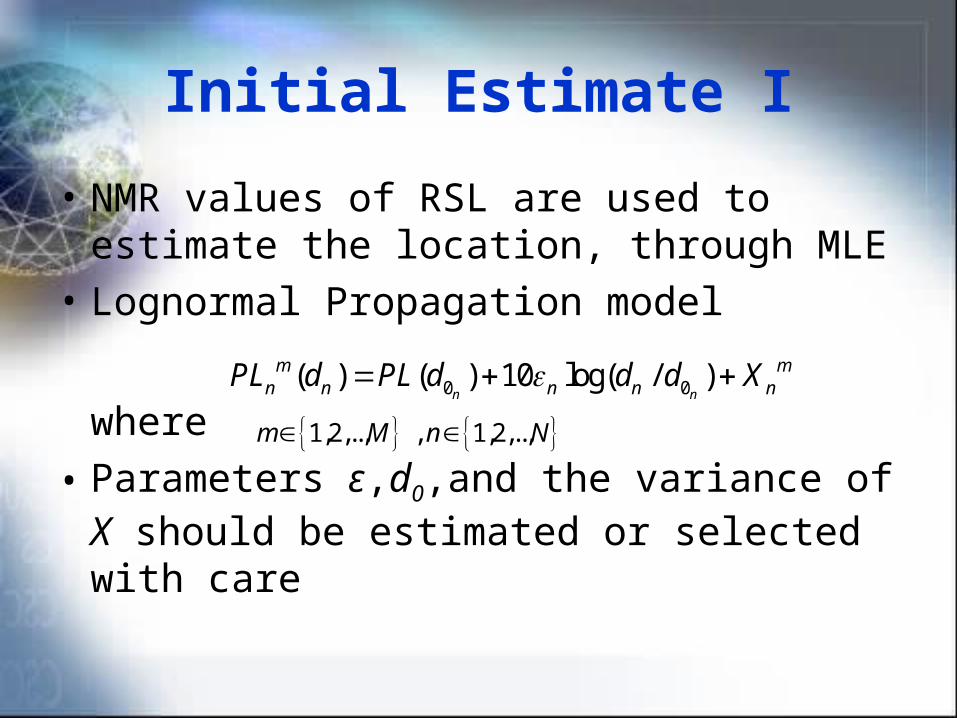
• NMR values of RSL are used to estimate the location, through MLE
• Lognormal Propagation model
where
• Parameters ε,d0,and the variance of X should be estimated or selected with care
0 0( ) ( ) 10 log( / )n n
m mn n n n nPL d PL d d d X
1,2,.., , 1,2,..,m M n N
Initial Estimate II
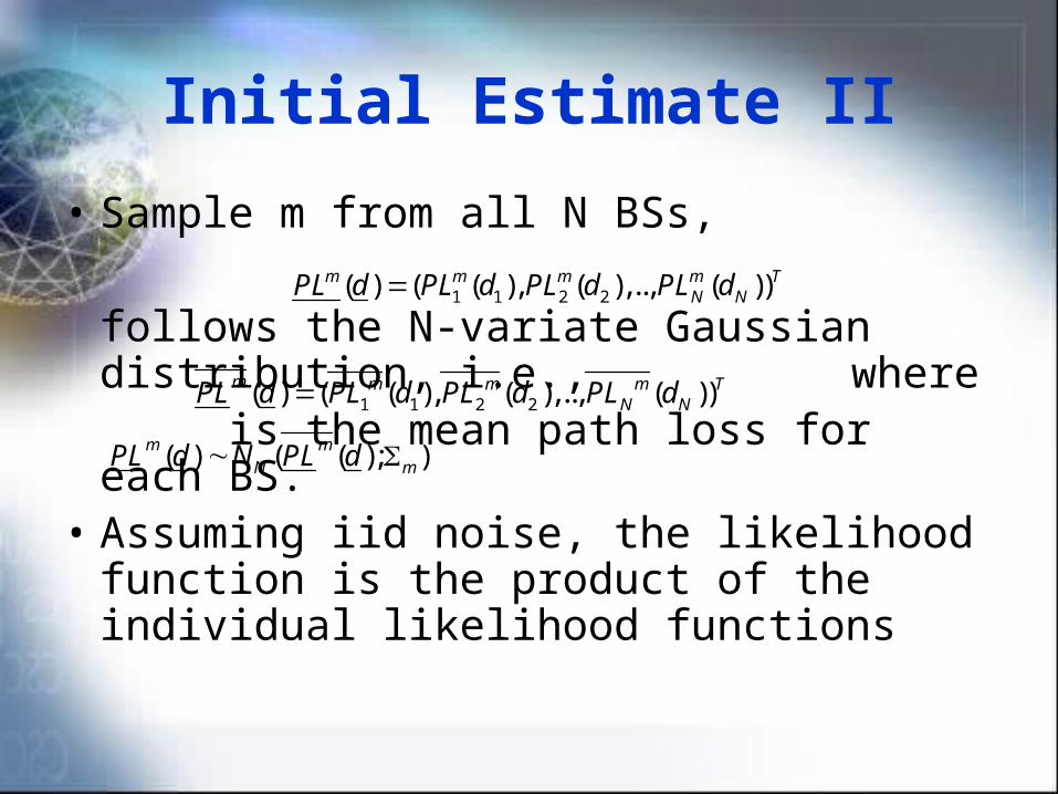
• Sample m from all N BSs,
follows the N-variate Gaussian distribution, i.e., where
is the mean path loss for each BS.
• Assuming iid noise, the likelihood function is the product of the individual likelihood functions
1 1 2 2( ) ( ( ), ( ),.., ( ))m m m m TN NPL d PL d PL d PL d
( ) ( ( ); )m mN mPL d N PL d
1 1 2 2( ) ( ( ), ( ),.., ( ))m m m m TN NPL d PL d PL d PL d
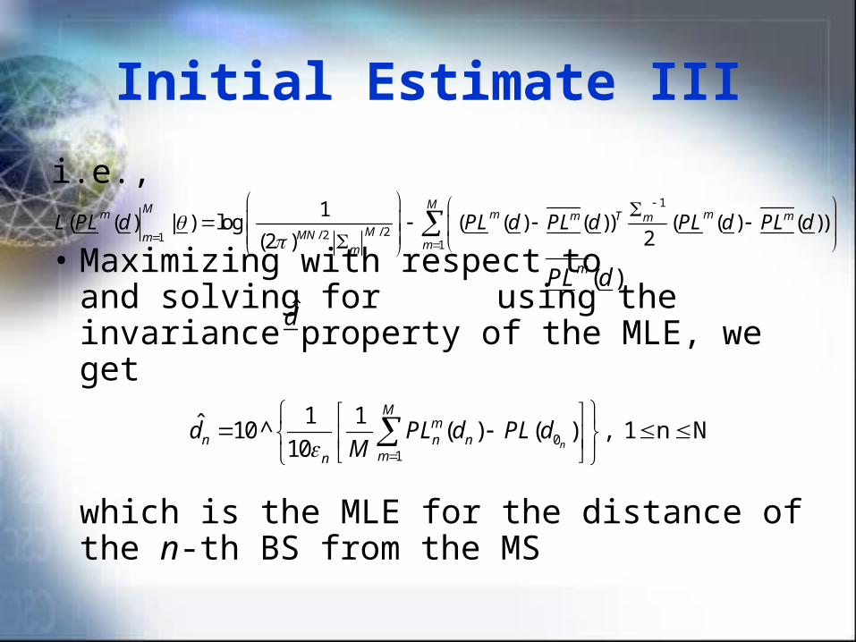
Initial Estimate III
i.e.,
• Maximizing with respect to and solving for using the invariance property of the MLE, we get
which is the MLE for the distance of the n-th BS from the MS
1
/ 2/ 211
1( ( ) | ) log ( ( ) ( )) ( ( ) ( ))
2(2 )
MMm m mm T mmMMNm
mm
L PL d PL d PL d PL d PL d
( )mPL d
d̂
01
1 1ˆ 10 ^ ( ) ( ) , 1 n N10 n
Mm
n n nmn
d PL d PL dM
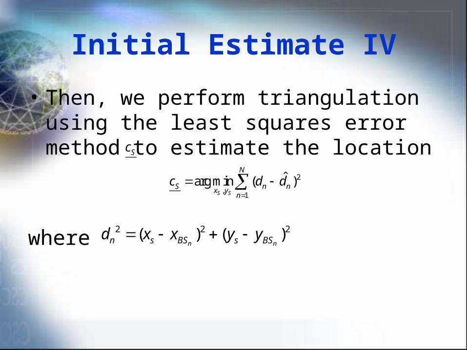
Initial Estimate IV
• Then, we perform triangulation using the least squares error method to estimate the location
where
Sc
2
,1
ˆarg min ( )S S
N
S n nx yn
c d d
2 2 2 ( ) ( )n nn s BS s BSd x x y y
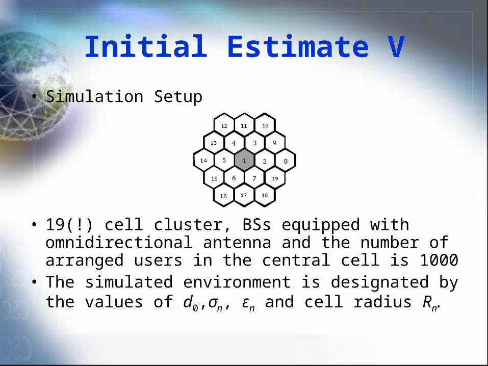
Initial Estimate V
• Simulation Setup
• 19(!) cell cluster, BSs equipped with omnidirectional antenna and the number of arranged users in the central cell is 1000
• The simulated environment is designated by the values of d0,σn, εn and cell radius Rn.
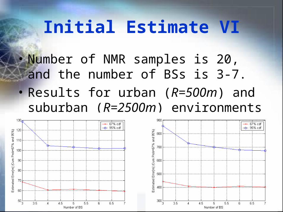
Initial Estimate VI
• Number of NMR samples is 20, and the number of BSs is 3-7.
• Results for urban (R=500m) and suburban (R=2500m) environments
Initial Estimate VII
• The FCC mandate is satisfied for urban environments only. Inconsistency of the method
• Main error source is triangulation. The error increases as the cell radius increases
• Failure as a stand-alone method BUT
• Localizes the problem
Final Estimate I
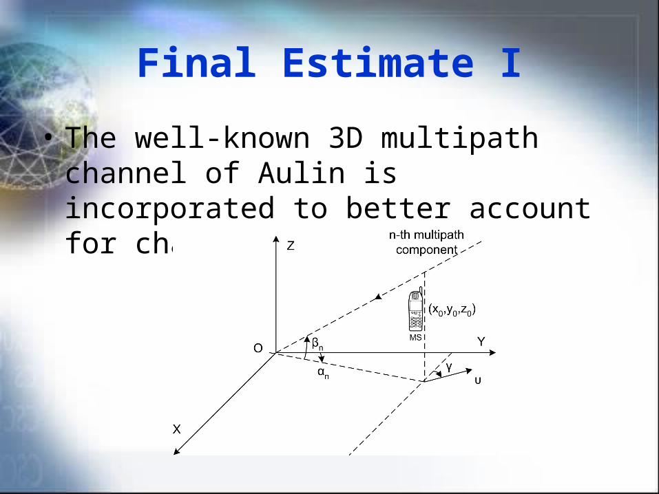
• The well-known 3D multipath channel of Aulin is incorporated to better account for channel impairments
Final Estimate II
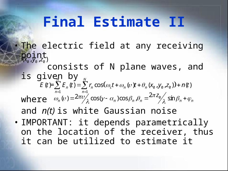
• The electric field at any receiving point consists of N plane waves, and is
given by
whereand n(t) is white Gaussian noise
• IMPORTANT: it depends parametrically on the location of the receiver, thus it can be utilized to estimate it
0 0 0( , , )x y z
0 0 01 1
( )= ( ) cos ( ) ( , , ) ( )N N
n n c n nn n
E t E t r t t x y z n t
022( ) cos( )cos , sinn n n n n nz
Final Estimate III
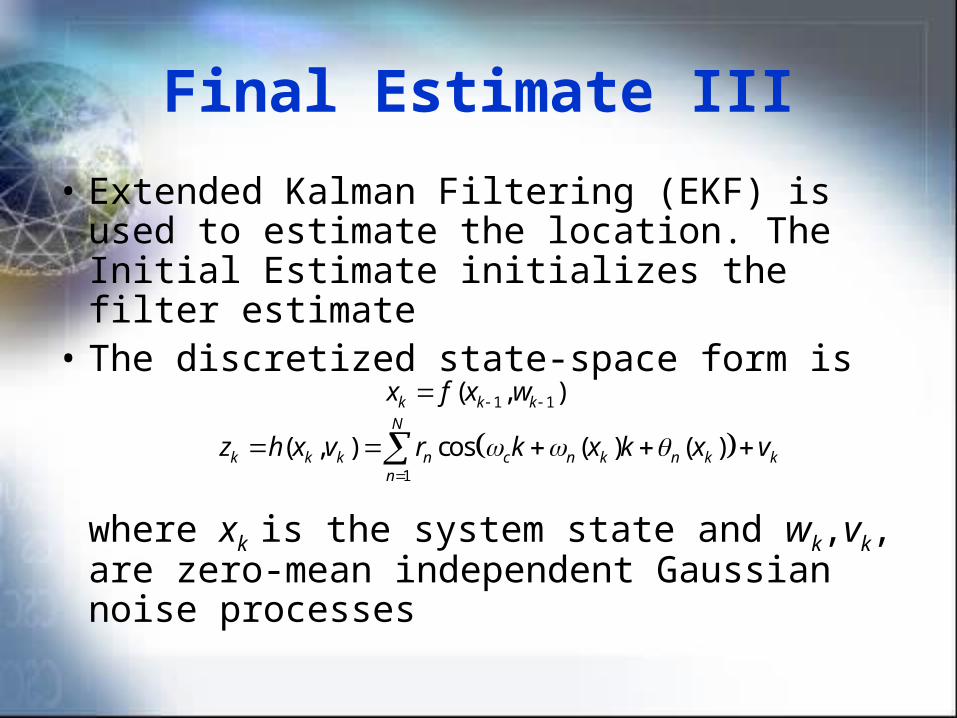
• Extended Kalman Filtering (EKF) is used to estimate the location. The Initial Estimate initializes the filter estimate
• The discretized state-space form is
where xk is the system state and wk,vk, are zero-mean independent Gaussian noise processes
1
( , ) cos ( ) ( )N
k k k n c n k n k kn
z h x v r k x k x v
1 1( , )k k kx f x w
Final Estimate IV
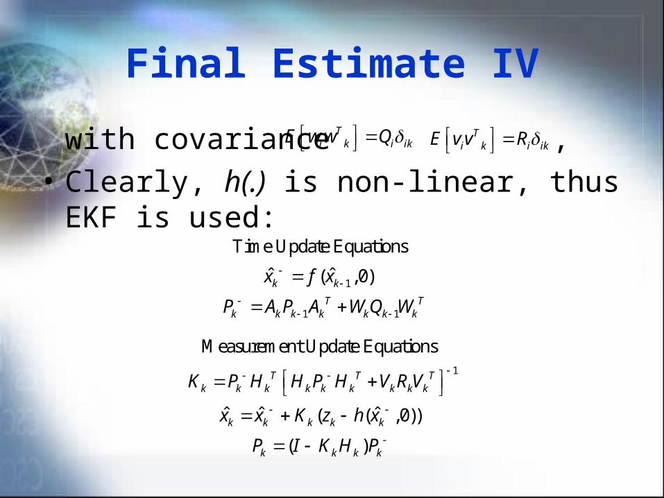
with covariance ,
• Clearly, h(.) is non-linear, thus EKF is used:
Ti k i ikE ww Q
Ti k i ikE v v R
1
1 1
Time Update Equations
ˆ ˆ ( ,0)
k k
T Tk k k k k k k
x f x
P A P A W Q W
1
Measurement Update Equations
ˆ ˆ ˆ ( ( ,0))
( )
T T Tk k k k k k k k k
k k k k k
k k k k
K P H H P H V R V
x x K z h x
P I K H P
Final Estimate V
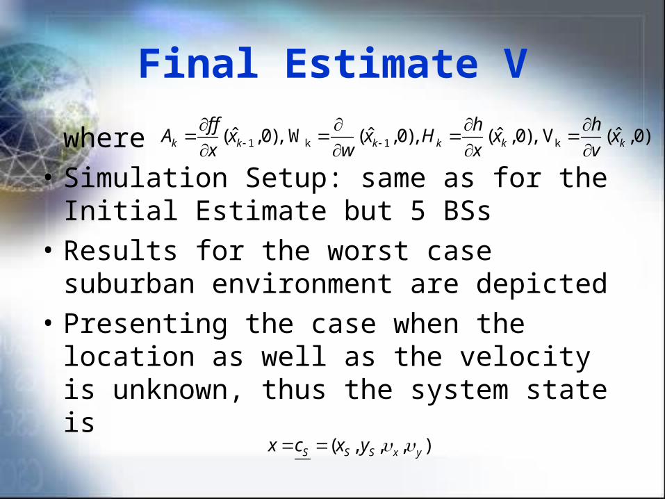
where
• Simulation Setup: same as for the Initial Estimate but 5 BSs
• Results for the worst case suburban environment are depicted
• Presenting the case when the location as well as the velocity is unknown, thus the system state is
1 k 1 kˆ ˆ ˆ ˆ( ,0), W ( ,0), ( ,0), V ( ,0)k k k k k k
f f h hA x x H x x
x w x v
( , , , )S S S x yx c x y
Final Estimate VI
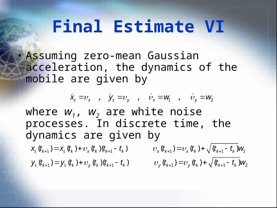
• Assuming zero-mean Gaussian acceleration, the dynamics of the mobile are given by
where w1, w2 are white noise processes. In discrete time, the dynamics are given by
1 2 , , , s x s y x yx y w w
1 1 1 1 1
1 1 1 1 2
( ) ( ) ( )( ) ( ) ( ) ( )
( ) ( ) ( )( ) ( ) ( ) ( )
s k s k x k k k x k x k k k
s k s k y k k k y k y k k k
x t x t t t t t t t t w
y t y t t t t t t t t w
Final Estimate VII
in which f(.) is a linear and A is a 4x4 identity matrix
• For urban areas we take with Rayleigh distributed attenuation. In urban and suburban areas we take N between 2-6 with Nakagami distributed attenuation
6N
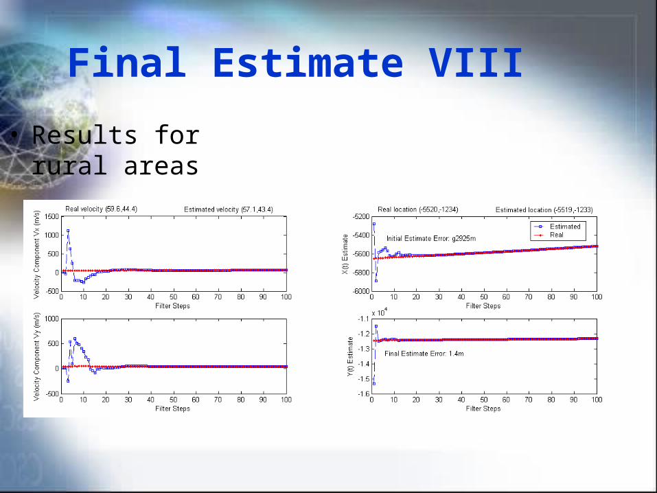
Final Estimate VIII
• Results for rural areas
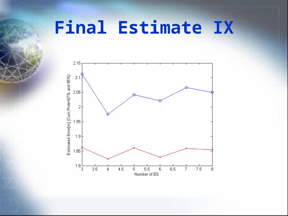
Final Estimate IX
Conclusions
• Triangulation is an obstacle for location estimation
• Stand-alone methods are not consistent
• The algorithmic part of a method is important for TTFF
• A method should be robust against channel knowledge
Recommended