An Insight Into Hydrocarbon Extraction From Shale:
Definitely Not A Geoscientist’s Bore Nor an Engineer’s Dream
Dr. Iain Bartholomew
Image from Norton et al, CSEG Recorder, 2011 (Progress Energy Resources)

Discussion outline
• Conventional versus unconventional
• Geology is the key to commerciality
• Breakthroughs in predicting the sweet-spots
• Enhancing production
• The North American shale story
• ….. and what about the UK?
2 Photos from: Hammes et al, AAPG Bulletin, 2011 (Bureau of Economic Geology)

Conventional v’s unconventional gas production
3
Typical gas recovered per well: 10 – 100
bcf
Typical production rate per well: 10 –
100 million scf/d
Typical gas recovered per well: 0.5 – 10
bcf
Typical production
rate per well: 1 – 10 million scf/d (30 day
IP rate) Data source: Drillinginfo
10 mmscf/d

• Typical dimensions - 1 to 3km horizontal length
- Down to 100m spacing
- 2 to 4km depth
- Up to 20 horizontal wells per pad
- Up to 40 frac stages per horizontal well
Shale exploitation
4 EIA 2012
Total website
National Energy Board, Canada 2009
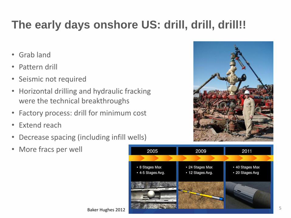
The early days onshore US: drill, drill, drill!!
• Grab land
• Pattern drill
• Seismic not required
• Horizontal drilling and hydraulic fracking were the technical breakthroughs
• Factory process: drill for minimum cost
• Extend reach
• Decrease spacing (including infill wells)
• More fracs per well
5 Baker Hughes 2012

Data from drillinginfo database
Huge variation in a single play: eg: Haynesville
Peak Gas Rate (mmscfpd/1,000ft, 30 Day Average) Average cumulative production per well (bcf)
• Peak gas rates range from 0 – 5 mmscfpd/1,000’
• Single wells produce 2.5 – 4.5 bcf during their life
6
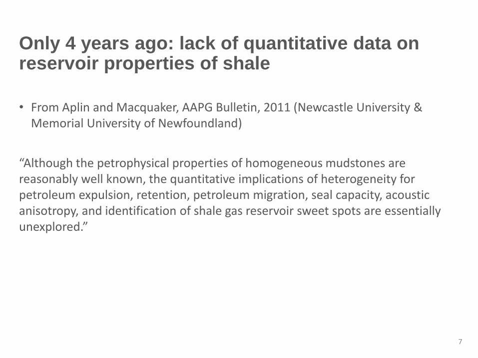
Only 4 years ago: lack of quantitative data on reservoir properties of shale
• From Aplin and Macquaker, AAPG Bulletin, 2011 (Newcastle University & Memorial University of Newfoundland)
“Although the petrophysical properties of homogeneous mudstones are reasonably well known, the quantitative implications of heterogeneity for petroleum expulsion, retention, petroleum migration, seal capacity, acoustic anisotropy, and identification of shale gas reservoir sweet spots are essentially unexplored.”
7

Geology is key to unconventional success
• Frackability
- Brittleness is good (quartz or calcite content)
- Clay is bad
- Fracture barriers (good or bad?)
- Natural fractures
• Hydrocarbon content and maturity
- High TOC good
- but high TOC is usually ductile rock (not good)
• Depth (> 5000 feet)
• Energy for production
- Pressure (small over-pressure is good)
• Structural complexity (simple is good)
- Understanding of regional stress important
• Regional geological understanding is essential
Photos from the Utica shale, Canada (A primer for understanding Canadian shale gas, National Energy Board, Canada, 2009)
8
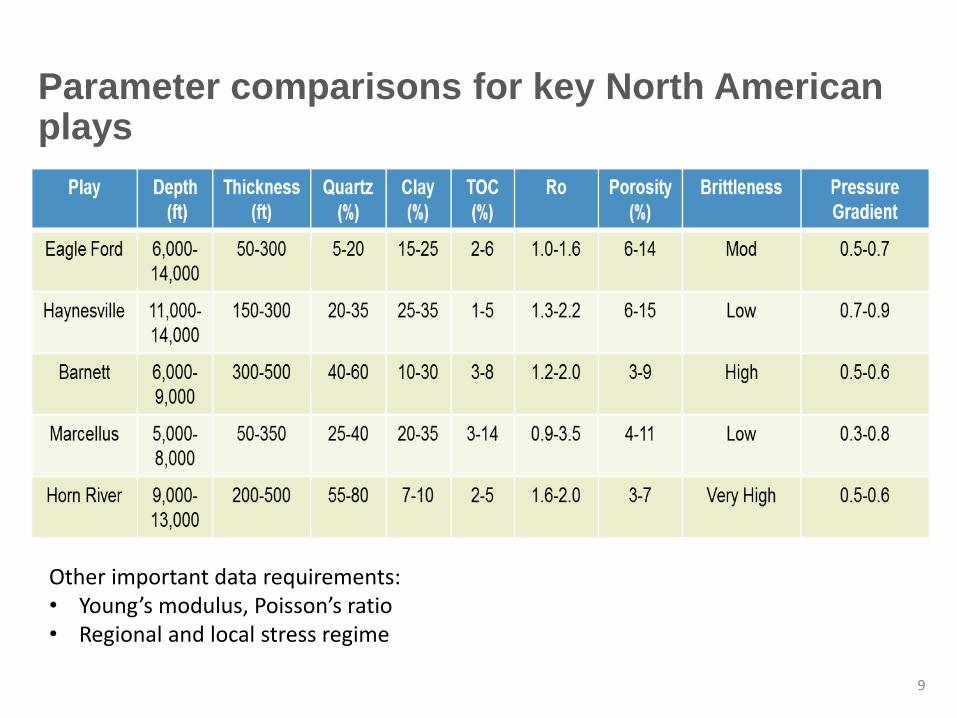
Parameter comparisons for key North American plays
9
Other important data requirements: • Young’s modulus, Poisson’s ratio • Regional and local stress regime

Mudstone diversity: key sedimentological considerations for source, seal, and reservoir properties in petroleum systems
10 From: Aplin and Macquaker, AAPG Bulletin, 2011 (Newcastle University & Memorial University of Newfoundland)
• Mineralogy
• Grain size
• Bioturbation
• Diagenetic changes (pre- and post-compaction)
- Including burial and uplift affects
• Depositional setting
- Suspension settling out from low-energy buoyant plumes
- But dispersed by a combination of waves, gravity-driven processes, and unidirectional currents driven variously by storms and tides
- Organised into packages that can be interpreted by sequence stratigraphy
Core slab of un-laminated
mudstone facies (arrow points to a bi-
valve)
Core slab of bioturbated mudstone facies with carbonate bioclasts
Photos from: Hammes et al, AAPG Bulletin, 2011 (Bureau of Economic Geology)
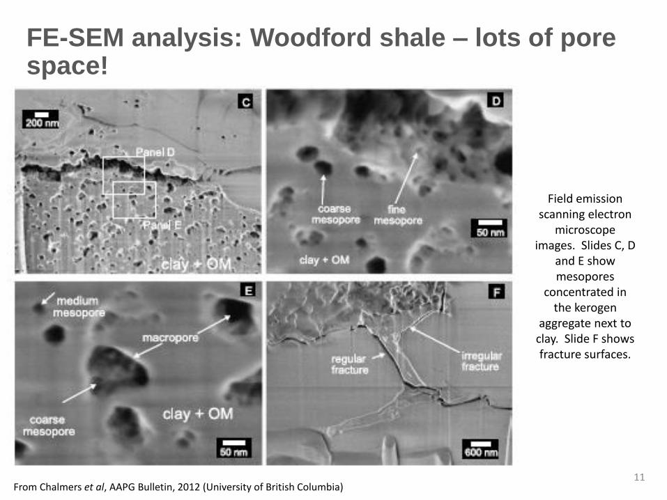
FE-SEM analysis: Woodford shale – lots of pore space!
11 From Chalmers et al, AAPG Bulletin, 2012 (University of British Columbia)
Field emission scanning electron
microscope images. Slides C, D
and E show mesopores
concentrated in the kerogen
aggregate next to clay. Slide F shows fracture surfaces.

Quantification of pore space in shale using nanometer-scale resolution imaging
12 From Curtis et al, AAPG Bulletin, 2012 (University of Oklahoma)
• Shales are quite different and their microstructures are highly variable and complex
• Understanding pore connectivity is key

Example of bioturbation enhancing reservoir quality
13 From: Bednarz and MacIlroy, AAPG Bulletin, 2012 (Memorial University of Newfoundland)
Core slab of bioturbated mudstone facies from Rosario Formation, Mexico (Mm =
mudstone matrix; Bc = burrow core composed of mineralogically altered clay
minerals; Bh = burrow halo composed of silt and sand grade minerals (mainly quartz).
3-D model of phycosiphoniform burrows from the Upper Cretaceous Rosario Formation, Mexico

Marcellus shale lithofacies modelling
14 From Wang and Carr, AAPG Bulletin, 2013 (West Virginia University)

Hybrid and stacked plays
• Hybrid plays contain organic rich shale intervals interbedded with gas charged silty layers.
• This is the case of the Montney formation in Western Canada, which contains a gradation of facies ranging from coastal sand to offshore shale and fine grained turbidites
• The deposition and preservation of organic matter in the sediments is a key element of the hydrocarbon system
15 From Pflug, NECA Conference, 2009 (TransCanada)
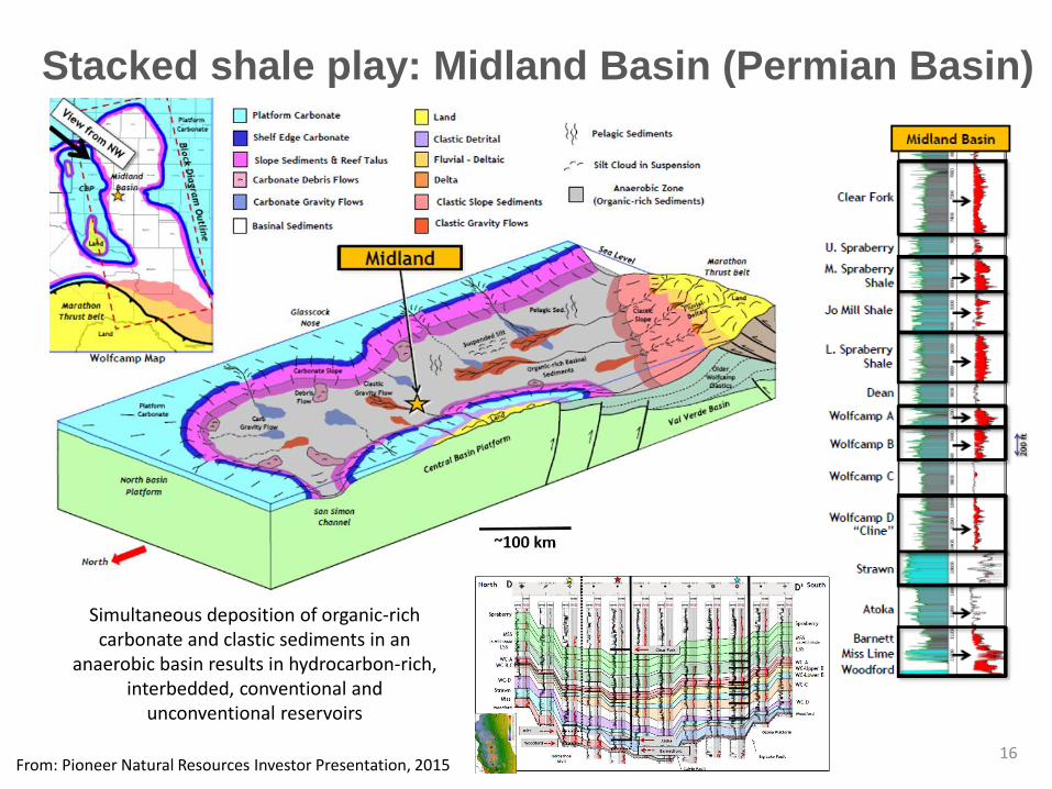
Stacked shale play: Midland Basin (Permian Basin)
16
Simultaneous deposition of organic-rich carbonate and clastic sediments in an
anaerobic basin results in hydrocarbon-rich, interbedded, conventional and
unconventional reservoirs
From: Pioneer Natural Resources Investor Presentation, 2015

Use of seismic data to predict reservoir quality in unconventional plays
• The two key properties derived from seismic for estimating ‘fracability’ are Young’s modulus and Poisson’s ratio
• Azimuthal inversion and AVO can be used to determine both the principal stresses and the differential horizontal stress ratio
• Faults and fracture identification from 3D volumes
• These data enable:
- Sweet spot identification
- Well location optimization
- Completions optimization
17 From Ouenes, CSEG Recorder, 2011 (Sigma3)
Niobrara shale, Teapot Dome, WY. Volumetric curvature map. Note: faulting changes to
folding where shale becomes more ductile.
2 km

Micro-seismic monitoring
18
Near-surface array design in the Horn River Basin. This array was used to monitor 253 fracking completions on a
10 well pad over a 90 day period.
From Snelling and Taylor, CSEG Recorder, 2013 (Microseismic Inc and Encana) and Norton et al, CSEG Recorder, 2011 (Progress Energy Resources)
Microseismic basic principle (vertical well)
Combined results from a 3 well fracking completion programme from Montney shale, Canada
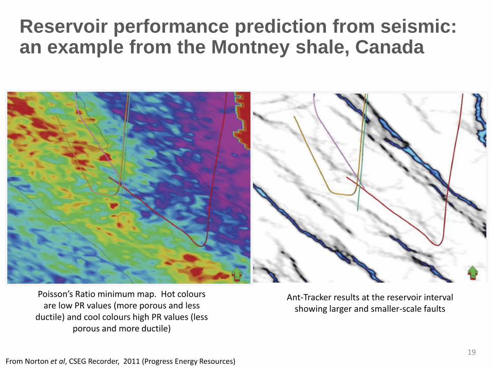
Reservoir performance prediction from seismic: an example from the Montney shale, Canada
19 From Norton et al, CSEG Recorder, 2011 (Progress Energy Resources)
Poisson’s Ratio minimum map. Hot colours are low PR values (more porous and less
ductile) and cool colours high PR values (less porous and more ductile)
Ant-Tracker results at the reservoir interval showing larger and smaller-scale faults

Reservoir performance prediction from seismic: micro-seismic data results from the Montney shale – evidence of fracture barriers
20 From Norton et al, CSEG Recorder, 2011 (Progress Energy Resources)
Map combining the PR minimum display with Ant-Tracker results at the reservoir interval, and the micro-seismic measurements from fracking (circle sizes
indicate magnitude of seismic event)

Better prediction of reservoir properties enables ‘informed’ production enhancement
• Infill Drilling
• Optimisation of well spacing
• Drilling longer laterals
• Offsets from existing laterals
• Optimising number of frac stages
• Simul fracs/Zipper fracs
• Refracs
• Managing drilling fluid chemistry
- avoid formation damage
- enhance brittleness and effectiveness of stimulation (including hydraulic fracturing)
21 Photos from American Oil & Gas Reporter, 2015

Unconventional oil and gas resources: the US story
22
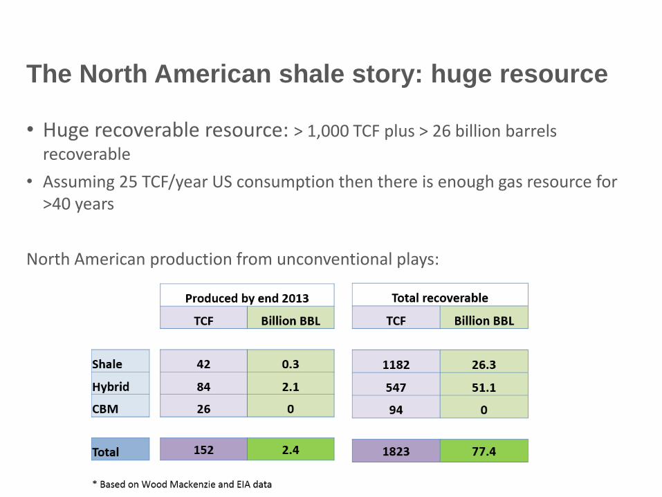
• Huge recoverable resource: > 1,000 TCF plus > 26 billion barrels
recoverable
• Assuming 25 TCF/year US consumption then there is enough gas resource for >40 years
North American production from unconventional plays:
The North American shale story: huge resource

The US shale story: its evolution
• Big tax incentives early on
- Federal Tax Section 29 nonconventional fuels production tax credit (on ‘tight’ wells drilled between 1980 – 1992)
• Lots of experimentation early on
- Antrim Shale: first development in 1965: 1,200 wells drilled in tax credit period (natural fractures)
3.3 TCF produced to date
- Barnett Shale: 275 vertical wells drilled in tax credit period. Slick water frac breakthrough in 1997. Horizontal development drilling starts in 2003. Experimentation continues in fracking
13 TCF produced to date
• Technological breakthroughs
- Horizontal drilling
- Hydraulic fracturing
24
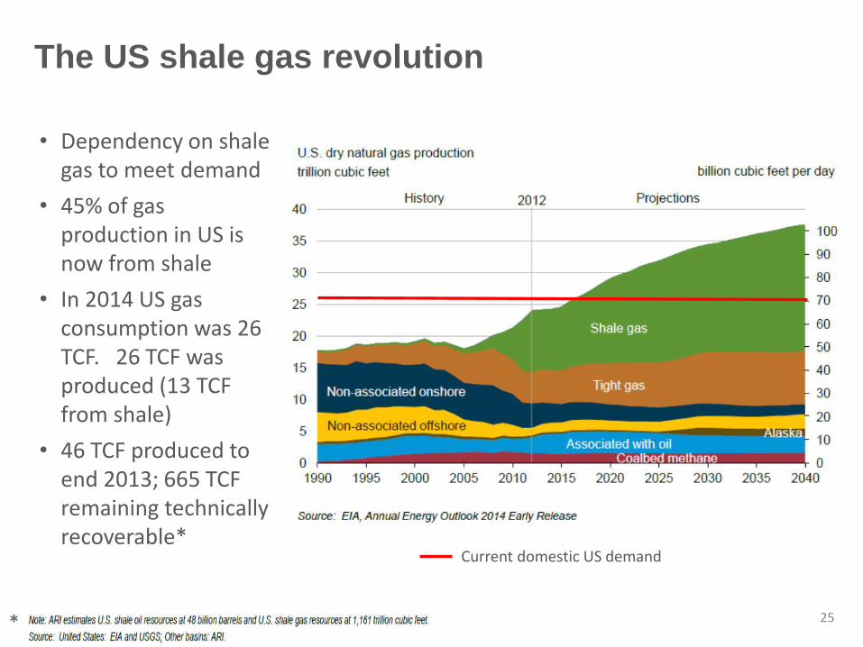
The US shale gas revolution
• Dependency on shale gas to meet demand
• 45% of gas production in US is now from shale
• In 2014 US gas consumption was 26 TCF. 26 TCF was produced (13 TCF from shale)
• 46 TCF produced to end 2013; 665 TCF remaining technically recoverable*
Current domestic US demand
25 *

…closely followed by oil from shale
26
• >50% of oil production in US is now from shale (~5.2 million barrels per day)
• In 2013 US oil consumption was 18.9 million barrels per day
• 58 billion barrels remaining technically recoverable*

US shale: scale of operations
• Huge scale of operation
- 1,700 land rigs in operation in US in early 2014: <1,000 in early 2015
- 36,000 wells drilled in 2013
- Over 30,000 wells are currently on production from shales
For oil on average each well produces 315 barrels oil per day
For gas on average each well produces 1.6 million standard cubic feet per day
• Very high level of drilling must continue in order to sustain production as individual wells only have 1- 5 year economic life
• Over 1 million wells required to produce unconventional resource in North America. 124,000 have already been drilled.
No. of horizontal wells drilled per year 1998 - 2012
~23,000 onshore
horizontal wells in
2013
27
Typical oil production from a single Bakken well

Where does it all come from?
• 64 key shale plays
• 28 are ‘pure shale’
• 36 are ‘hybrid’
• Huge variation in liquids content
28

0
20
40
60
80
100
120
140
160
180
200
TCFE
Ultimate recoverable reserves and produced reserves per play in Nth Am
Ultimately recoverable Produced to end 2013
Some plays have huge resources
Hybrid gas plays Liquid-rich shale plays Shale gas plays
Hybrid liquid-rich plays
425
Marcellus
Haynesville
Horn River
Eagle Ford
Duvernay
Cotton Valley
Montney
Bakken
Three Forks
Fayetteville
Liard
Barnett
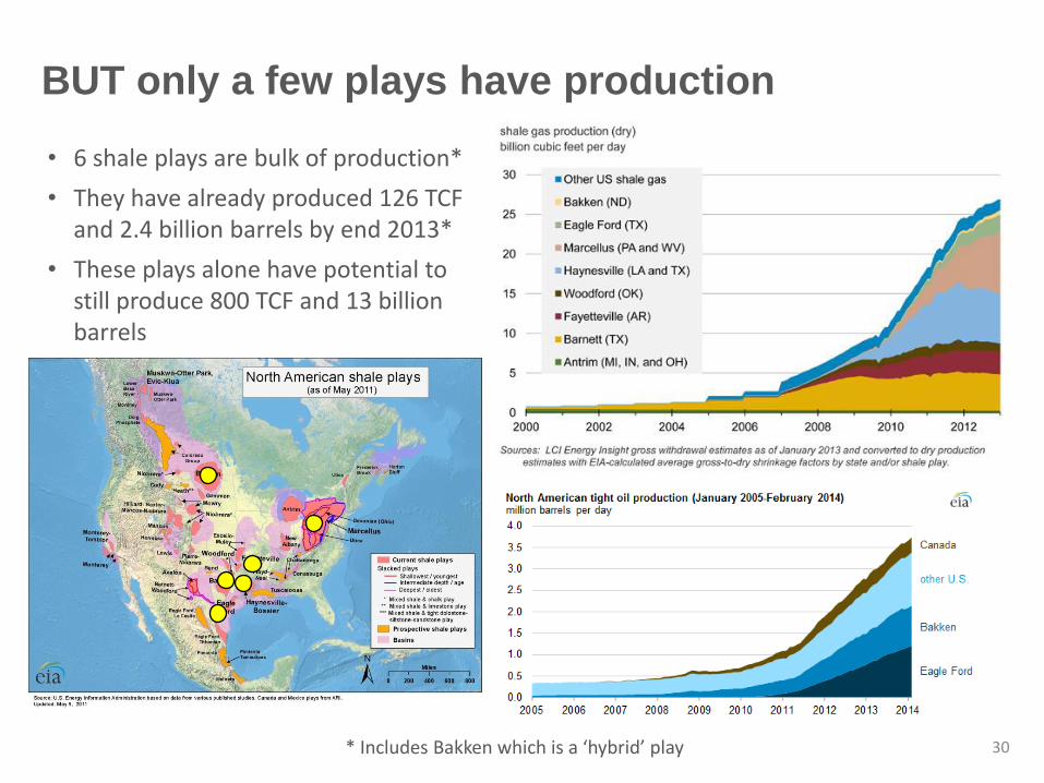
BUT only a few plays have production
• 6 shale plays are bulk of production*
• They have already produced 126 TCF and 2.4 billion barrels by end 2013*
• These plays alone have potential to still produce 800 TCF and 13 billion barrels
* Includes Bakken which is a ‘hybrid’ play 30
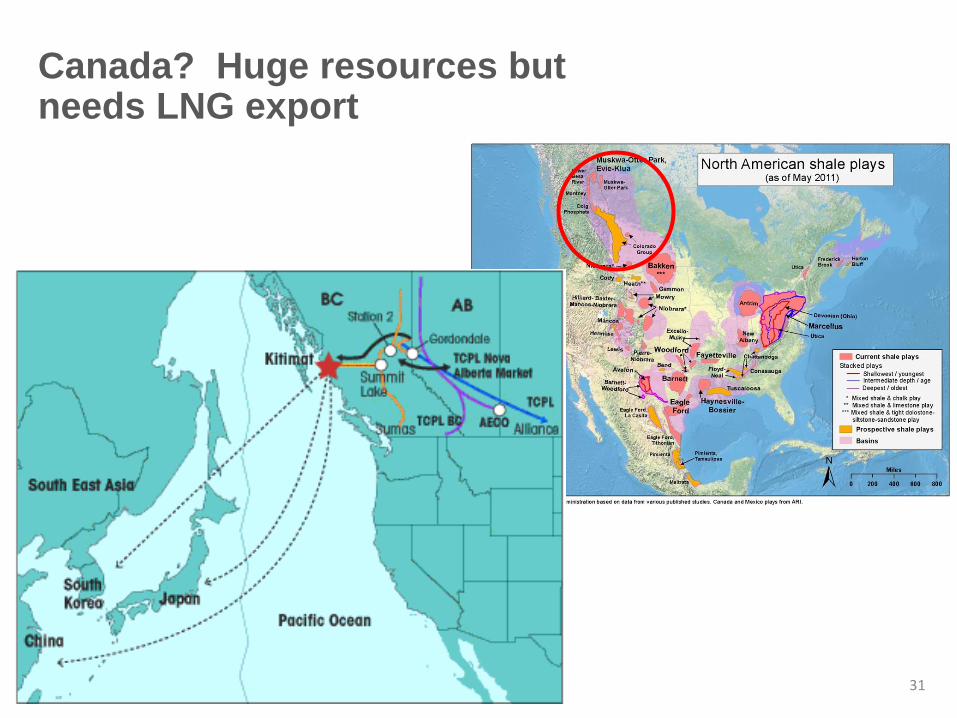
Canada? Huge resources but needs LNG export
31

Impact of the oil price crash
32

Oil price crash has materially impacted the number of active onshore drilling rigs
33
Baker Hughes
From Evercore ISI Investment Conference, 2015 (Pioneer Natural Resources)

Individual well productivity is enabling the industry to survive in a low price environment
34 From EIA, Drilling Productivity Report, May 2015

The UK Opportunity
35
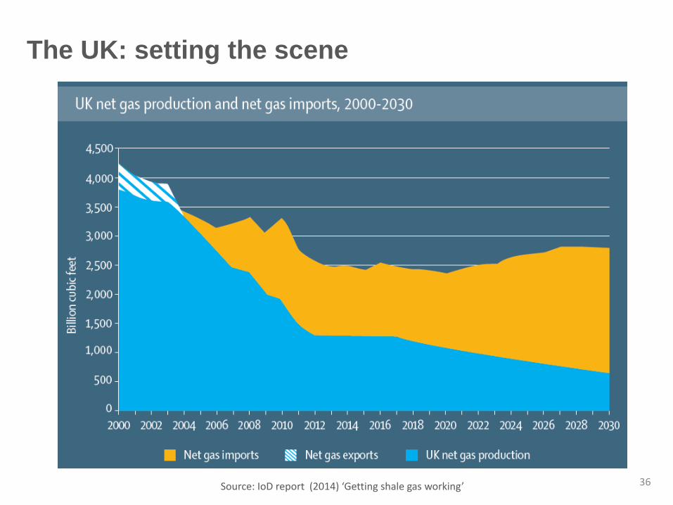
The UK: setting the scene
Source: IoD report (2014) ‘Getting shale gas working’ 36
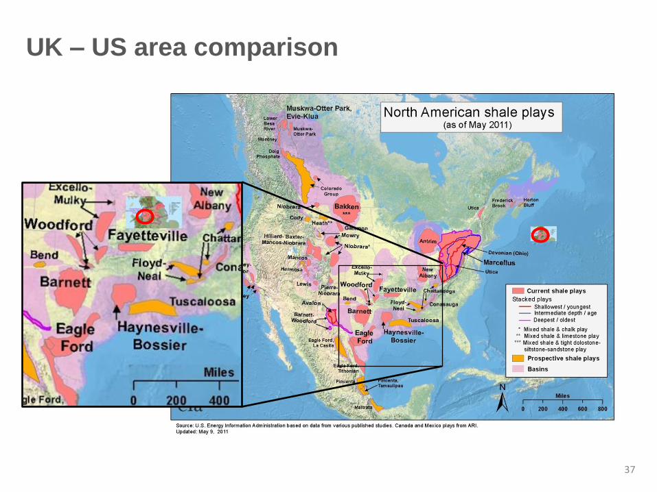
UK – US area comparison
37

UK: how do we compare?
• Very small areas compared to North America
• Structurally complex basins
• Much thicker shale sequences and therefore volumes could still be interesting
• BGS/DECC estimate ~1,300 TCF GIIP for Bowland (P50)
- BUT ??? recovery factor and commerciality
• In the UK we are still very much in the EXPLORATION stage – we will have to wait and see
• We can learn a huge amount from North America
From Andrews (2013) The Carboniferous Bowland Shale gas study: geology and resources estimation. BGS/DECC
38

39
ANY QUESTIONS?
Recommended


![Welcome [sites.nationalacademies.org] · Development of Unconventional Hydrocarbon Resources in the Appalachian Basin (DELS, ongoing) Health Impact Assessment of Shale Gas Extraction](https://img.pdfslide.net/doc/110x75/5fd6278f4d987d0e226382d5/welcome-sites-development-of-unconventional-hydrocarbon-resources-in-the-appalachian.jpg)