Our expertise is your advantage Company confidential
Analysis of Chilton Ionosonde Critical Frequency
Measurements During Solar Cycle 23 in the Context
of Midlatitude HF NVIS Frequency Predictions
(Use of T-Index with VOACAP)
Marcus C. Walden
HFIA Meeting, York, UK
6 September 2012
Our expertise is your advantage Company confidential
Overview of Presentation
• Introduction
• Motivation for this work
• MUF definitions
• HF propagation predictions
• Chilton ionosonde measurements
• Comparison methodology
• Results
• Summary
Our expertise is your advantage Company confidential
Introduction
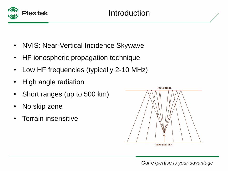
• NVIS: Near-Vertical Incidence Skywave
• HF ionospheric propagation technique
• Low HF frequencies (typically 2-10 MHz)
• High angle radiation
• Short ranges (up to 500 km)
• No skip zone
• Terrain insensitive
Our expertise is your advantage Company confidential
Motivation for this Work (1)
• Follow on from IET IRST 2009
– Relevance (and limitations) of extraordinary-wave (x-wave) in
NVIS propagation
– HF monthly-median prediction software (e.g. ASAPS, VOACAP)
considers x-wave for zero-distance MUF prediction
• Follow on from IET IRST 2012
– Chilton ionosonde critical frequency measurements
– ASAPS and VOACAP MUF predictions
– Upper and lower decile predictions
– Time period 1996-2010 (covering solar cycle 23)
Our expertise is your advantage Company confidential
Motivation for this Work (2)
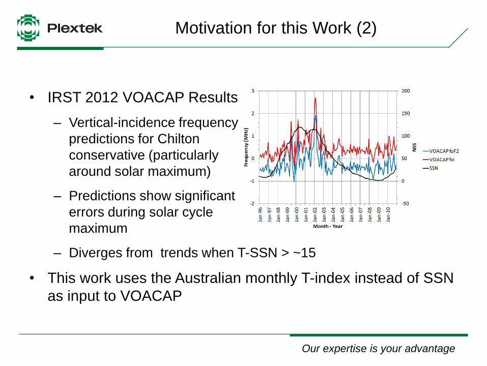
• IRST 2012 VOACAP Results
– Vertical-incidence frequency
predictions for Chilton
conservative (particularly
around solar maximum)
– Predictions show significant
errors during solar cycle
maximum
– Diverges from trends when T-SSN > ~15
• This work uses the Australian monthly T-index instead of SSN
as input to VOACAP
Our expertise is your advantage Company confidential
MUF Definitions (1)
• ITU-R Recommendation P.373-8
– Definitions of maximum and minimum transmission frequencies
• MUF – Maximum useable frequency
• Basic MUF
– Ionospheric refraction alone
• Operational MUF
– Considers system parameters
(e.g. transmit power, antenna gains, modulation, noise, etc.).
• Basic and operational MUF are median values
Our expertise is your advantage Company confidential
MUF Definitions (2)
• Optimum working frequency (OWF)
– Frequency exceeded by operational MUF during 90% of
specified period (usually a month)
• Highest probable frequency (HPF)
– Frequency exceeded by operational MUF during 10% of
specified period (usually a month)
• ITU-R Rec. P.373 places emphasis on ‘operational’
Our expertise is your advantage Company confidential
HF Prediction Software (1)
• ASAPS (Advanced Stand Alone Prediction System)
– Version 5.4
– GRAFEX predictions
– Monthly T-index (effective sunspot number)
Our expertise is your advantage Company confidential
HF Prediction Software (2)
• VOACAP (Voice of America Coverage Analysis Program)
– Version 09.1208
– Method 9 (HPF-MUF-FOT graph)
– International smoothed sunspot number (SSN)
• SSN is 12-month running mean value
• Recommended by George Lane for use with VOACAP
– Evaluate monthly T-index with VOACAP
Our expertise is your advantage Company confidential
HF Prediction Software (3)
• Global foF2 maps
– Sunspot numbers of 0 and 100
– Interpolation for different sunspot numbers
– IPS-own foF2 maps (ASAPS)
– CCIR coefficients (VOACAP)
• Predictions for median, upper and lower decile frequencies
– MUF, UD and OWF (ASAPS)
– MUF, HPF and FOT (VOACAP)
Our expertise is your advantage Company confidential
HF Prediction Software (4)
• ASAPS (GRAFEX) and VOACAP (Method 9) predictions
relate to basic MUF
– Not operational MUF
• Analysis presented here relates to basic MUF
• Knowledge of basic MUF does not guarantee successful link
– Link budget analysis required
Our expertise is your advantage Company confidential
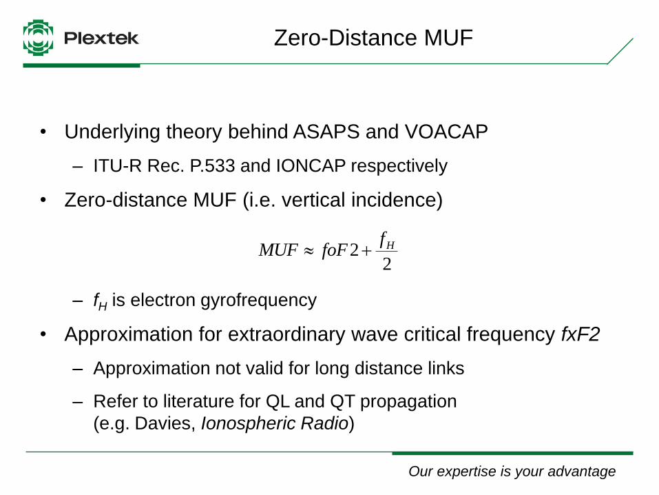
Zero-Distance MUF
• Underlying theory behind ASAPS and VOACAP
– ITU-R Rec. P.533 and IONCAP respectively
• Zero-distance MUF (i.e. vertical incidence)
– fH is electron gyrofrequency
• Approximation for extraordinary wave critical frequency fxF2
– Approximation not valid for long distance links
– Refer to literature for QL and QT propagation
(e.g. Davies, Ionospheric Radio)
22 HffoFMUF
Our expertise is your advantage Company confidential
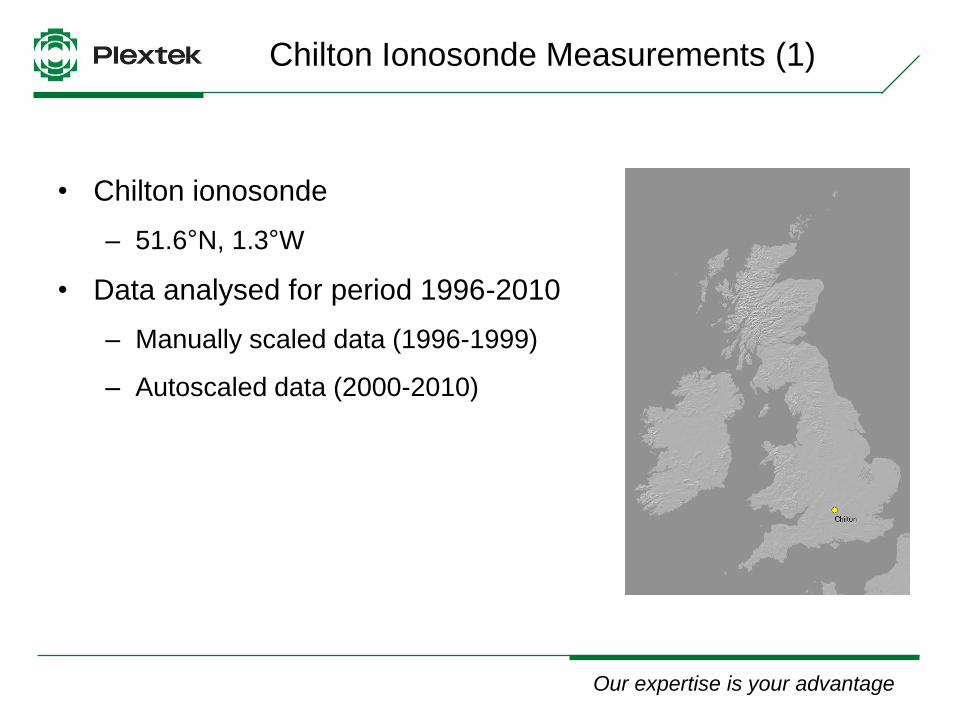
Chilton Ionosonde Measurements (1)
• Chilton ionosonde
– 51.6°N, 1.3°W
• Data analysed for period 1996-2010
– Manually scaled data (1996-1999)
– Autoscaled data (2000-2010)
Our expertise is your advantage Company confidential
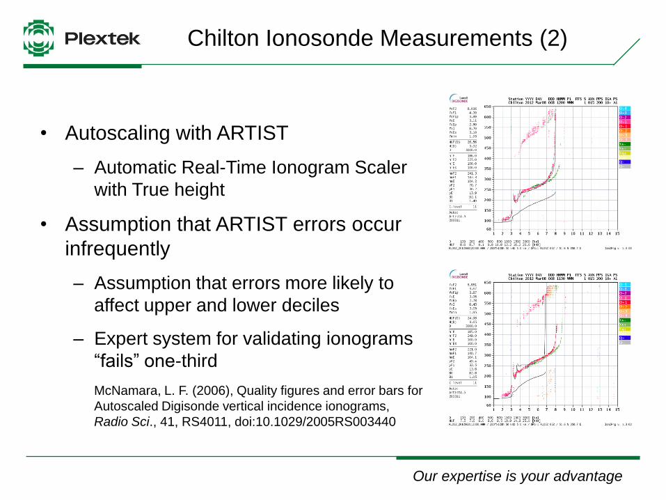
Chilton Ionosonde Measurements (2)
• Autoscaling with ARTIST
– Automatic Real-Time Ionogram Scaler
with True height
• Assumption that ARTIST errors occur
infrequently
– Assumption that errors more likely to
affect upper and lower deciles
– Expert system for validating ionograms
“fails” one-third
McNamara, L. F. (2006), Quality figures and error bars for
Autoscaled Digisonde vertical incidence ionograms,
Radio Sci., 41, RS4011, doi:10.1029/2005RS003440
Our expertise is your advantage Company confidential
Chilton Ionosonde Measurements (3)
• Critical frequency measurements
– foF2
– fxF2 (not a standard ionogram output parameter)
• Spread F Index, fxI
– Maximum F region frequency recorded
– Measure of spread F associated with overhead ionosphere
• When spread F is uncommon
– Median fxI equal to median fxF2
• For this analysis, fxI used in lieu of fxF2
Our expertise is your advantage Company confidential
Chilton Ionosonde Measurements (4)
• Sounding rates varied from 1996 to 2010
– Hourly in 1996
– Every 10 minutes in 2010
• Ionosonde measurements grouped according to timestamp
– Time rounded to nearest hour
– Comparison with ASAPS and VOACAP hourly predictions
• Calculated for each hour
– Median foF2 and median fxI
– Upper and lower decile values (10% and 90%) for foF2 and fxI
Our expertise is your advantage Company confidential
Comparison Methodology
• Measurements compared with predictions
– Median (MUF)
– Upper decile (UD/HPF)
– Lower decile (OWF/FOT)
• Matrix of differences for each hour of each month
– Mean and standard deviation
• Assess
– Diurnal variation
– Month-to-month variation
– Overall performance (1996-2010)
Our expertise is your advantage Company confidential
Comment on Results
• Conclusions from this work specific to Chilton
– More generally the UK
• ASAPS and VOACAP predictions depend on non-identical
global foF2 maps
• Absolute/relative prediction errors depend on geomagnetic
location
Our expertise is your advantage Company confidential
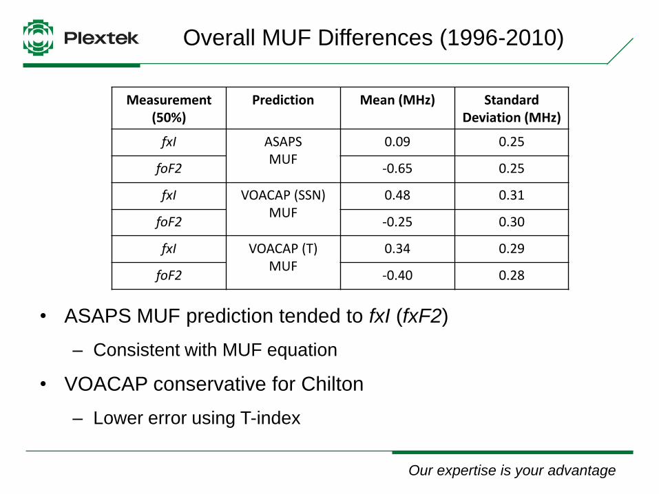
Overall MUF Differences (1996-2010)
• ASAPS MUF prediction tended to fxI (fxF2)
– Consistent with MUF equation
• VOACAP conservative for Chilton
– Lower error using T-index
Measurement (50%)
Prediction Mean (MHz) Standard Deviation (MHz)
fxI ASAPS MUF
0.09 0.25
foF2 -0.65 0.25
fxI VOACAP (SSN) MUF
0.48 0.31
foF2 -0.25 0.30
fxI VOACAP (T) MUF
0.34 0.29
foF2 -0.40 0.28
Our expertise is your advantage Company confidential
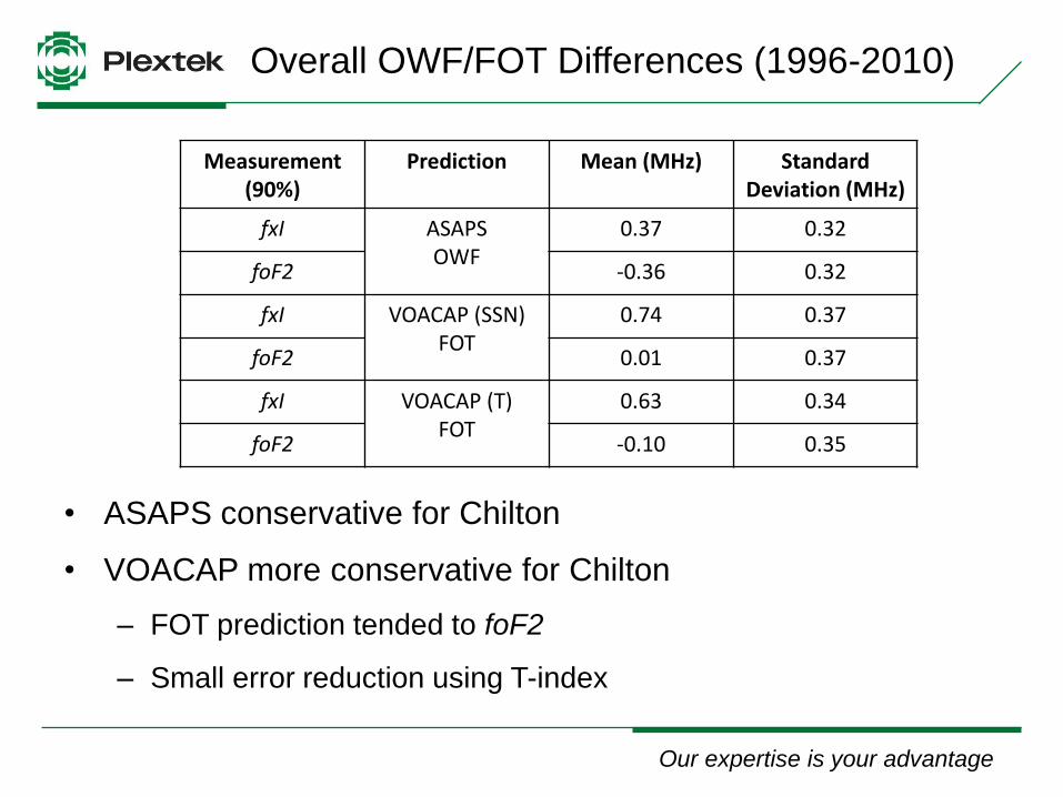
Overall OWF/FOT Differences (1996-2010)
• ASAPS conservative for Chilton
• VOACAP more conservative for Chilton
– FOT prediction tended to foF2
– Small error reduction using T-index
Measurement (90%)
Prediction Mean (MHz) Standard Deviation (MHz)
fxI ASAPS OWF
0.37 0.32
foF2 -0.36 0.32
fxI VOACAP (SSN) FOT
0.74 0.37
foF2 0.01 0.37
fxI VOACAP (T) FOT
0.63 0.34
foF2 -0.10 0.35
Our expertise is your advantage Company confidential
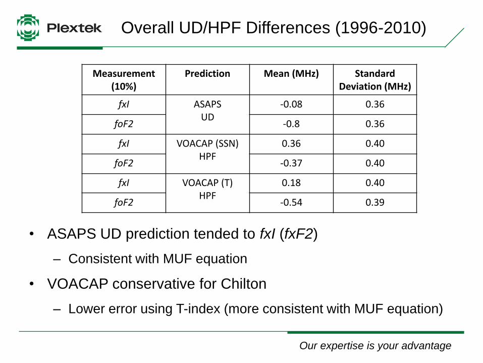
Overall UD/HPF Differences (1996-2010)
• ASAPS UD prediction tended to fxI (fxF2)
– Consistent with MUF equation
• VOACAP conservative for Chilton
– Lower error using T-index (more consistent with MUF equation)
Measurement (10%)
Prediction Mean (MHz) Standard Deviation (MHz)
fxI ASAPS UD
-0.08 0.36
foF2 -0.8 0.36
fxI VOACAP (SSN) HPF
0.36 0.40
foF2 -0.37 0.40
fxI VOACAP (T) HPF
0.18 0.40
foF2 -0.54 0.39
Our expertise is your advantage Company confidential
Results – ALE Frequency Planning
• ALE frequency planning (George Lane)
– Follow diurnal maximum observed frequency (MOF) variation
– Minimum frequency below lowest FOT/OWF
– Maximum frequency close to maximum HPF/UD
• ASAPS might be better than VOACAP for generating UK ALE
frequency scan lists
– Based on overall results
– VOACAP overall results show lower error using monthly T-index
• CAUTION – Still require full link budget analysis
Our expertise is your advantage Company confidential
Results – Monthly Variation (1)
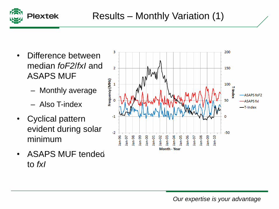
• Difference between
median foF2/fxI and
ASAPS MUF
– Monthly average
– Also T-index
• Cyclical pattern
evident during solar
minimum
• ASAPS MUF tended
to fxI
Our expertise is your advantage Company confidential
Results – Monthly Variation (2)
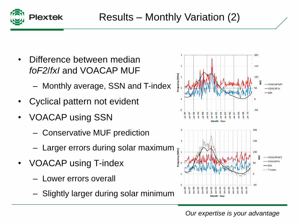
• Difference between median
foF2/fxI and VOACAP MUF
– Monthly average, SSN and T-index
• Cyclical pattern not evident
• VOACAP using SSN
– Conservative MUF prediction
– Larger errors during solar maximum
• VOACAP using T-index
– Lower errors overall
– Slightly larger during solar minimum
Our expertise is your advantage Company confidential
Results – Monthly Variation (3)
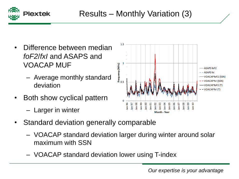
• Difference between median
foF2/fxI and ASAPS and
VOACAP MUF
– Average monthly standard
deviation
• Both show cyclical pattern
– Larger in winter
• Standard deviation generally comparable
– VOACAP standard deviation larger during winter around solar
maximum with SSN
– VOACAP standard deviation lower using T-index

Our expertise is your advantage Company confidential
Results – Monthly Variation (4)
• Cyclical pattern
– Difficulty predicting F2 region ‘winter anomaly’
• VOACAP solar maximum discrepancies
– ASAPS uses monthly T-index
– VOACAP uses SSN (12-month running mean)
– ‘Ersatz’ indices (e.g. T-index) outperform direct indices
(e.g. SSN)
– Sunspot number is only circumstantial index
i.e. no physical basis for direct relationship between sunspot
number and ionospheric response

Our expertise is your advantage Company confidential
Results – Variation over Year 2002 (1)
• Difference between
median fxI and ASAPS
MUF (2002)
• Large positive
differences day and night
during winter and early
spring
• Some months in 2002
show negative
differences during day
and night
Our expertise is your advantage Company confidential
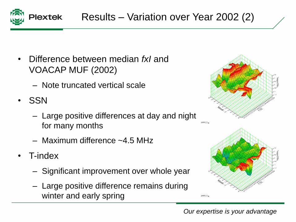
Results – Variation over Year 2002 (2)
• Difference between median fxI and
VOACAP MUF (2002)
– Note truncated vertical scale
• SSN
– Large positive differences at day and night
for many months
– Maximum difference ~4.5 MHz
• T-index
– Significant improvement over whole year
– Large positive difference remains during
winter and early spring
Our expertise is your advantage Company confidential
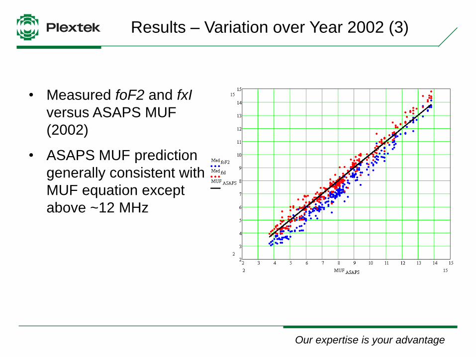
Results – Variation over Year 2002 (3)
• Measured foF2 and fxI
versus ASAPS MUF
(2002)
• ASAPS MUF prediction
generally consistent with
MUF equation except
above ~12 MHz
Our expertise is your advantage Company confidential
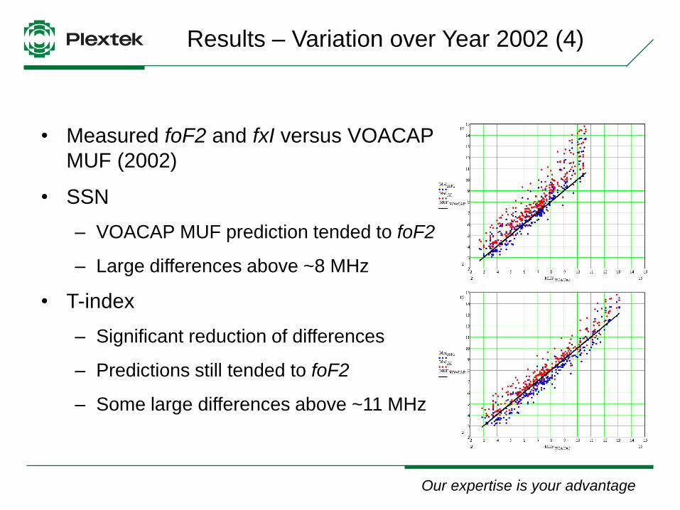
Results – Variation over Year 2002 (4)
• Measured foF2 and fxI versus VOACAP
MUF (2002)
• SSN
– VOACAP MUF prediction tended to foF2
– Large differences above ~8 MHz
• T-index
– Significant reduction of differences
– Predictions still tended to foF2
– Some large differences above ~11 MHz
Our expertise is your advantage Company confidential
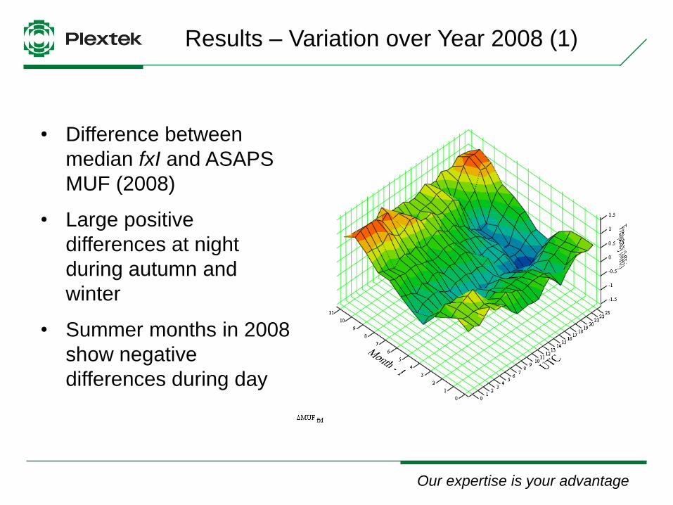
Results – Variation over Year 2008 (1)
• Difference between
median fxI and ASAPS
MUF (2008)
• Large positive
differences at night
during autumn and
winter
• Summer months in 2008
show negative
differences during day
Our expertise is your advantage Company confidential
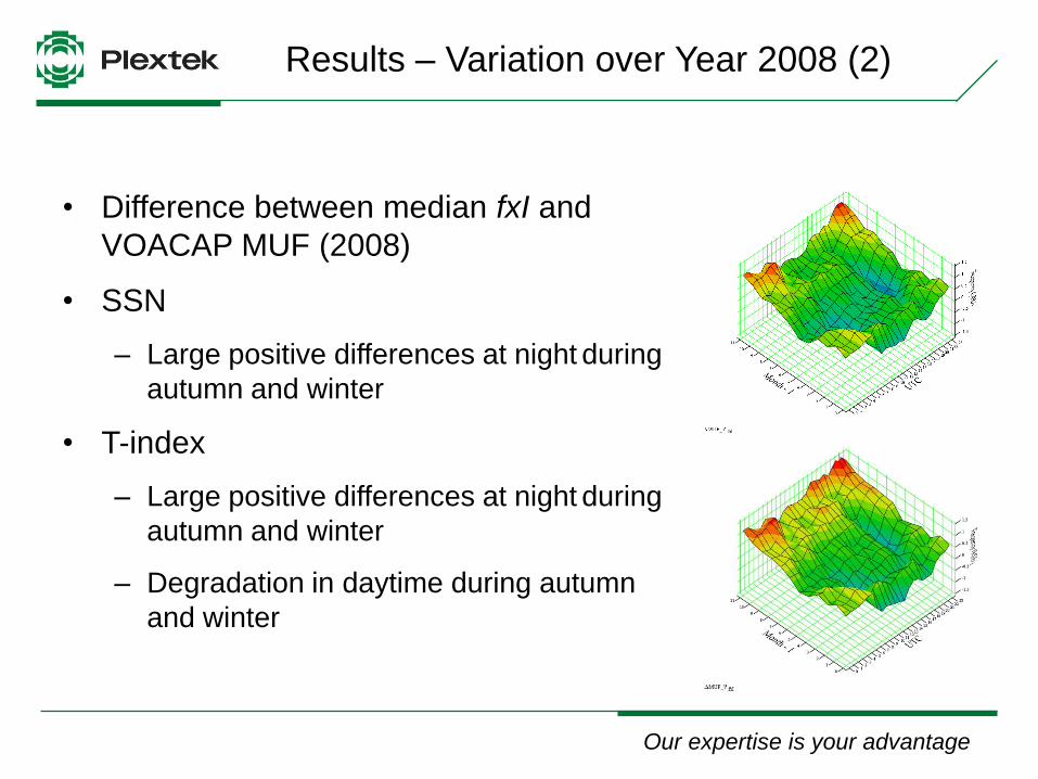
Results – Variation over Year 2008 (2)
• Difference between median fxI and
VOACAP MUF (2008)
• SSN
– Large positive differences at night during
autumn and winter
• T-index
– Large positive differences at night during
autumn and winter
– Degradation in daytime during autumn
and winter
Our expertise is your advantage Company confidential
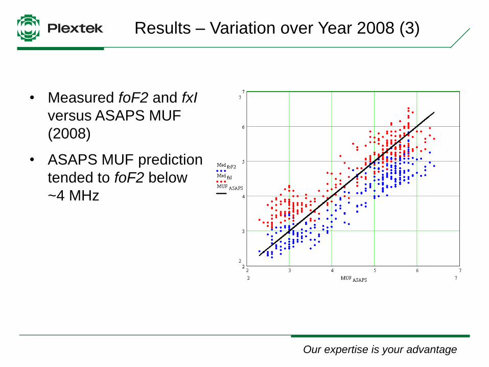
Results – Variation over Year 2008 (3)
• Measured foF2 and fxI
versus ASAPS MUF
(2008)
• ASAPS MUF prediction
tended to foF2 below
~4 MHz

Our expertise is your advantage Company confidential
Results – Variation over Year 2008 (4)
• Measured foF2 and fxI versus VOACAP
MUF (2008)
• Both SSN and T-index
– VOACAP MUF prediction tended to foF2
below ~4 MHz
• T-index
– Less consistent with MUF equation
Our expertise is your advantage Company confidential
Results – Variation over Year 2008 (5)
• Development of IONCAP
– George Lane
“There was very little data below 4 MHz but there was some for
short paths that did go down to 2 MHz.”
• IONCAP developers modelled a fit to these cases
– Understood to have given good results for NVIS situations
• Presumably, this also applies for REC533 and ASAPS
Our expertise is your advantage Company confidential
Results – Variation over Year 2008 (6)
• Errors in foF2 maps
• Errors due to ionogram autoscaling
– Chilton autoscaled foF2 measurements show positive errors at
LF
• Bamford, R. A., R. Stamper, and L. R. Cander (2008), A comparison
between the hourly autoscaled and manually scaled characteristics
from the Chilton ionosonde from 1996 to 2004, Radio Sci., 43,
RS1001, doi:10.1029/2005RS003401
• Spread F
– High-latitude spread F begins at ~40° geomagnetic latitude
– High-latitude spread F occurs mostly at night
Our expertise is your advantage Company confidential
Results – Solar Indices (1)
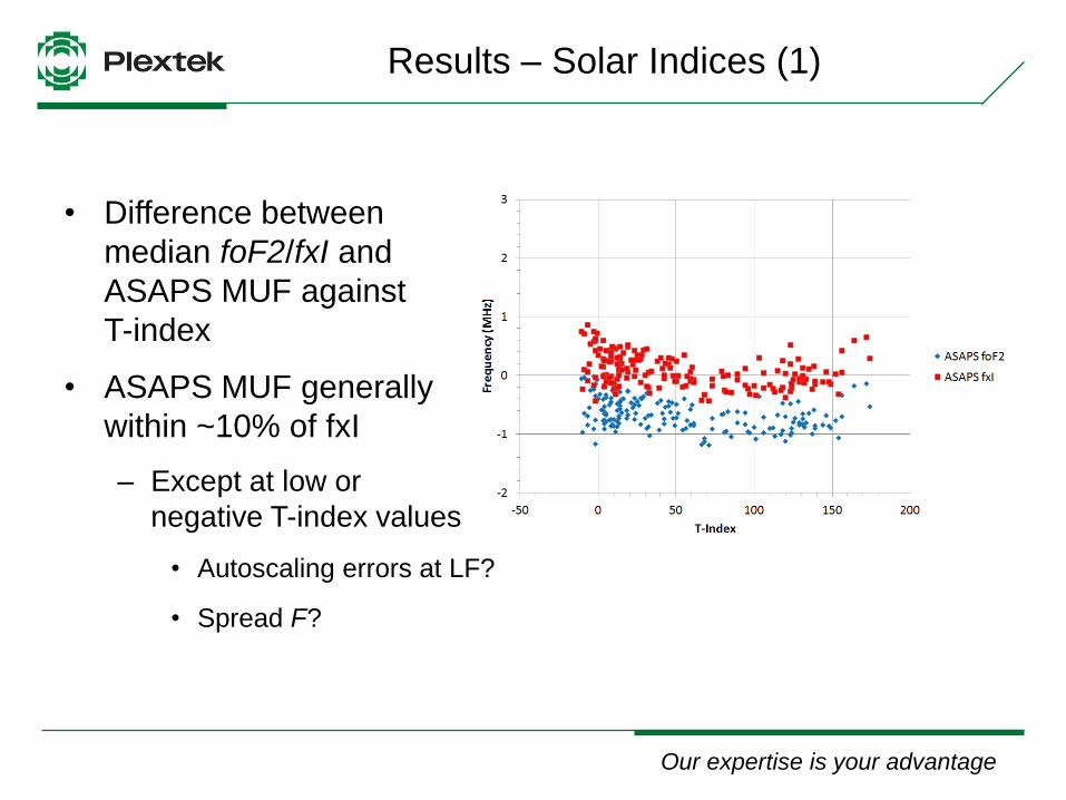
• Difference between
median foF2/fxI and
ASAPS MUF against
T-index
• ASAPS MUF generally
within ~10% of fxI
– Except at low or
negative T-index values
• Autoscaling errors at LF?
• Spread F?
Our expertise is your advantage Company confidential
Results – Solar Indices (2)
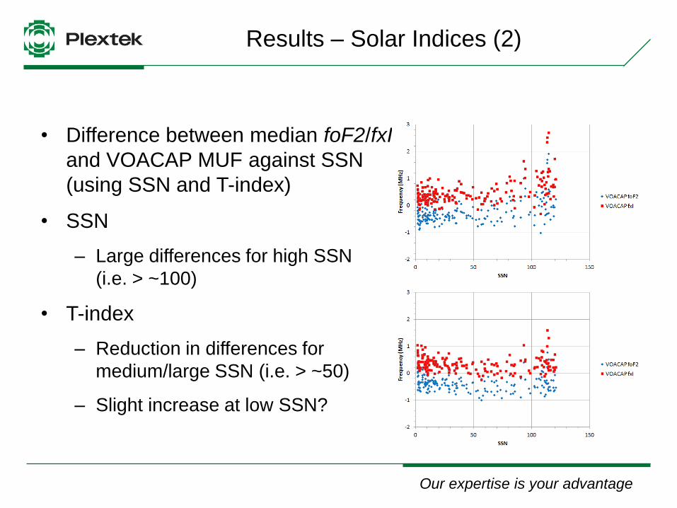
• Difference between median foF2/fxI
and VOACAP MUF against SSN
(using SSN and T-index)
• SSN
– Large differences for high SSN
(i.e. > ~100)
• T-index
– Reduction in differences for
medium/large SSN (i.e. > ~50)
– Slight increase at low SSN?

Our expertise is your advantage Company confidential
Results – Solar Indices (3)
• Difference between median foF2/fxI
and VOACAP MUF against T-SSN
• SSN
– VOACAP diverges from trends
when T-SSN > ~15
– Identifies periods when Chilton/UK
NVIS basic MUF predictions might
be inaccurate (or pessimistic)
• T-index
– Lower differences for T-SSN > 0
– Slight increase for T-SSN < 0?
Our expertise is your advantage Company confidential
Results – Solar Indices (4)
• VOACAP predictions might be inaccurate (or pessimistic) for
Chilton/UK NVIS basic MUF predictions when T-SSN > ~15
– Assumes real-time access to T-index
• Averaging of effective sunspot number?
• 5-day average “strikes a good balance” (John M. Goodman )
• IPS provide 7-day average
• During solar maximum
– Consider effective sunspot number instead of SSN in VOACAP
• During solar minimum
– Use SSN in VOACAP

Our expertise is your advantage Company confidential
Summary (1)
• Conclusions specific to Chilton (more generally the UK)
• For the period 1996-2010
– ASAPS basic MUF predictions generally agreed with Chilton fxI
measurements
– ASAPS MUF prediction consistent with zero-distance MUF
equation
– VOACAP predictions conservative (particularly around solar
maximum)
– Similar observations for upper decile (10%) predictions
– ASAPS and VOACAP lower decile (90%) predictions
conservative (VOACAP more so)
Our expertise is your advantage Company confidential
Summary (2)
• Below ~4 MHz during winter nights around solar minimum
– ASAPS and VOACAP MUF predictions tended towards foF2
– Contrary to underlying theory
– Autoscaling errors due to nighttime spread F?
• ASAPS errors increased at low or negative T-index values
– Autoscaling errors due to nighttime spread F?
• VOACAP errors
– Greatest at solar maximum using SSN
– Errors might be large when T-SSN exceeds ~15
– Errors reduced when using T-index
Our expertise is your advantage Company confidential
Acknowledgements
• UK Solar System Data Centre, RAL Space
– Allowing the use of Chilton ionosonde data
• George Lane
– Archiving a paper copy of the Nacaskul reference
(now available at the DTIC)
Recommended