ANALYSIS OF COLOUR DISPLAY CHARACTERISTICS
Behnam Bastani B.Sc Computing Science, Simon Fraser University, 2003
THESIS SUBMITTED IN PARTIAL FULFILLMENT OF THE REQUIREMENTS FOR THE DEGREE OF
MASTER OF SCIENCE
In the School of Computing Science
O Behnam Bastani, 2005
SIMON FRASER UNIVERSITY
Spring 2005
All rights reserved. This work may not be reproduced in whole or in part, by photocopy
or other means, without permission of the author.
APPROVAL
Name:
Degree:
Title of Thesis:
Behnam Bastani
Master of Science
ANALYSIS OF COLOUR DISPLAY CHARACTERISTICS
Examining Committee:
Chair: Dr. Greg Mori Assistant Professor of Computing Science
Dr. Brian Funt Senior Supervisor Professor of Computing Science
Date DefendedJApproved:
Dr. Ghassan Hamarneh Supervisor Assistant Professor of Computing Science
Dr. Tim Lee
Internal Examiner Adjunct Professor of Computing Science
Simon Fraser University
SIMON FRASER UNIVERSITY
PARTIAL COPYRIGHT LICENCE
The author, whose copyright is declared on the title page of this work, has granted to Simon Fraser University the right to lend this thesis, project or extended essay to users of the Simon Fraser University Library, and to make partial or single copies only for such users or in response to a request from the library of any other university, or other educational institution, on its own behalf or for one of its users.
The author has further granted permission to Simon Fraser University to keep or make a digital copy for use in its circulating collection.
The author has further agreed that permission for multiple copying of this work for scholarly purposes may be granted by either the author or the Dean of Graduate Studies.
It is understood that copying or publication of this work for financial gain shall not be allowed without the author's written permission.\
Permission for public performance, or limited permission for private scholarly use, of any multimedia materials forming part of this work, may have been granted by the author. This information may be found on the separately catalogued multimedia material and in the signed Partial Copyright Licence.
The original Partial Copynght Licence attesting to these terms, and signed by this author, may be found in the original bound copy of this work, retained in the Simon Fraser University Archive.
W. A. C. Bennett Library Simon Fraser University
Bumaby, BC, Canada

ABSTRACT
Predicting colours across multiple display devices requires implementation of
device characterization, gamut mapping, and perceptual models. This thesis studies
characteristics of CRT, LCD monitors and projectors. It compares existing models and
introduces a new model that improves existing calibration algorithms.
Gamut mapping assigns a mapping between two different colour spaces.
Previously, the focus of gamut mapping has been between monitor and printer, which
have relatively different gamut shape. Implementation and result of existing models are
compared and a new model is introduced that its output images are as good as the best
available models but runs in less time.
DLP projectors with a different technology require a more complex calibration
algorithm. A new approach for calibrating DLP projectors is introduced with a
significantly better performance on predicting RGB data given tristimulus values.
At the end, a new calibration method, using Support Vector Regression is
introduced.

DEDICATION
I dedicate this work to my awesome parents:
Bijan Bastani and Mahnaz Gheibi
for their time and support.

ACKNOWLEDGEMENTS
I would like to thank Brian Funt for his support and guidance in this thesis and
Ghassan Hamarneh for supervising me. My great friends, Roozbeh Ghaffari and Bill
Cressman, are my great friends that helped me a lot. At last, I would like to thank my
parents Bijan and Mahnaz for their constant support throughout my school time.

TABLE OF CONTENTS
.. Approval ............................................................................................................................ n ... Abstract ............................................................................................................................. 111
Dedication ....................................................................................................................... iv
Acknowledgements ............................................................................................................ v
............................................................................................................. Table of Contents vi ...
List of Figures ................................................................................................................. v ~ n
List of Tables ................................................................................................................. xii
List of Abbreviations ..................................................................................................... xiv
Chapter 1: Introduction .................................................................................................... 1
........................................................................................ Chapter 2: Display Calibration 5 .................................................................................. Calibration Introduction 5
................................................................................................ Data Collection 7 ................................................................................. Device Characteristics 1 2 ................................................................................. Implementation Details 17
3D LUT Model .......................................................................................... 17 Linear Model ............................................................................................. 17
.......................................................................................... Masking Model 22 Calibration Results ........................................................................................ 25
................................................................ Summary of the Calibration Study 29
Chapter 3: Optimal Device Calibration ......................................................................... 34 .................................................................................................. Introduction -34
.................................................. CIELAB Weighted Least Squares (LabLS) 35 ............................................................................... AE Minimization (DEM) 36 . . ......................................................................... Measurement Charactenstics 36
.......................................................................................................... Results -36 ...................................................... Summary of Optimal Device Calibration 38
Chapter 4: Gamut Mapping for Electronic Displays ................................................... 39 ........................................................................ 4.1 Gamut Mapping Introduction 39
......................................... 4.2 Characteristics of LCD and CRT Display Gamut 41 .............................................................................................. 4.2.1 Gamut Shape 41 . .
4.2.2 Predicting Out of Gamut ............................................................................ 45 4.2.3 Using Convex-Hull Algorithm to Predict Gamut Boundary ..................... 45
4.3 Known Device-dependant GMAs ................................................................. 46

.................................................................................. Methods of Mapping 47 ................................................................................ Direction of Mapping 50
Results of Device-based GMAs .................................................................... 53 ........................................................................... Clipping Implementation 53
................................. Non-linear Compression Mapping, Implementation 54 ............................... Combination of Linear Transformation and Clipping 58
.................................................................... Content Based Gamut Mapping 61 ...... Gamut Mapping to Preserve Spatial Luminance Variations: Bala [7] 63
Space Sensitive Colour Gamut Mapping: Kimmel ................................... 67 Summary of Gamut Mapping ........................................................................ 79
............................................................................................... Chapter 5: DLP Projector 82 ..................................................................... 5.1 DLP Technology. Introduction -82
5.2 DLP Projector Characteristic ......................................................................... 84 ........................................................................... 5.3 Calibrating DLP Projectors 86
............................................................... 5.3.1 Linear Model for DLP Projector 87 ................................................................. 5.3.2 Number of Channels Required -88
......................................... 5.3.3 Wyble's Model for DLP Projector Calibration 90 ........................................................................... 5.3.4 Modified Wyble Method 94
......................................................................................... 5.3.5 Masking Model -94 ............................................................................ 5.3.6 DLP Calibration Results 95
.................................................................. 5.3.7 Summary of DLP Calibration 101 .................................................................................. 5.4 DLP Projector Gamut 102
....................................................... Chapter 6: Lcd Projector Versus DLP Projector 107 ....................................................................................... 6.1 Temporal Stability 107
....................................................................... 6.2 Spatial Non-Uniformity [42] 109
Chapter 7: Device Calibration via Support Vector Regression ................................. 112 ................................................................................................. 7.1 Introduction 112
...................................................... 7.2 Applying SVR to Calibration Problem 1 4 ......................................................................................................... 7.3 Results 115
Chapter 8: Conclusion ................................................................................................... 117
Chapter 9: Contribution Summary .............................................................................. 120
Reference List ................................................................................................................. 122
vii

LIST OF FIGURES
Figure 2-1 : Percentage of the steady state luminance for white on the vertical axis versus the number of seconds since black was displayed on the horizontal axis. .............................................................................................. .9
Figure 2-2: Measurement Error (Log scale) versus integration time in milliseconds ................................................................ measured for four greys on CRTl 1 1
Figure 2-3: Channel Interaction. The horizontal axis represents the input value v ranging from 0 to 255 and the vertical axis represents the value of the channel interaction metric, CICOLOR(v,a,b). The black line shows a=b=255 and dashed lines show a=O,b=255 and a=255,b=0 ....................... 14
Figure 2-4
Figure 2-5
Figure 2-6
Figure 2-7
Figure 2-8
Figure 2-9
Chromaticity shift shown as intensity is increased plotted in xy space with x=X/(X+Y+Z) on the horizontal axis and y=Y/(X+Y+Z) on the vertical axis. When there is no chromaticity shift, all the dots of one colour lie on top of one another and therefore appear as a single dot. ......... 16
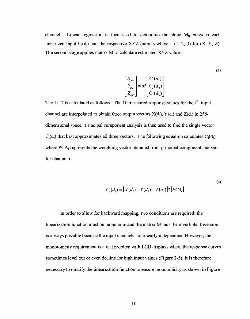
Luminance curves for red, green, and blue phosphor input (Horizontal .............................. axis: R, G or B value. Vertical axis: L from CIELAB) 19
Smoothing correction for non-monotonicity in the Z-response curve of the B channel for PR1. The vertical axis is the Z value reading and horizontal axis represents the digital counts for blue from 0 to 255 ............ 20
Mapping Error versus Training Data Size .................................................... 21
Backward Error distribution for each characterization model on each device. AE error value is shown on the horizontal axis and histogram counts are shown on the vertical axis. .......................................................... 3 1
Comparison of Outliers for the Backward model. Vertical axis and horizontal axes represent Y./(X+Y+Z) and X./(X+Y+Z) respectively. The AE error is plotted according to the legend of grey scales. The circular points represent outliers with AE greater than 1.5 times the average error. The majority of the high outlier errors for LUT model occur near the gamut boundaries. . The outliers for Linear Model are quite negligible compared to the other two models. .................................... 32
Figure 2- 10 Linearization failure for the black channel on PR1 ...................................... 33
Figure 4-1 Gamut shape of Displays in XYZ space ...................................................... 43
.................................................. Figure 4-2 Gamut shape of displays in L*a*b* space -44
viii
Figure 4-3
Figure 4-4
Figure 4-5
Figure 4-6
Figure 4-7
Figure 4-8
Figure 4-9
Figure 4- 10
Figure 4- 1 1
Figure 4- 12
Figure 4- 13
Figure 4- 14
Figure 4- 15
Gamut clipping and compression along a given direction. Target represent Target Gamut boundary and Source is the source (original) gamut boundary [ 1 31 . ..... . . . . . . . . . . . . . . . . . . . . . . . . . . . . . . . . . . . . . . . . . . . . . . . . . . . . . . . . . . . . . . . . . . . . . . . . . . . . . -49
Directions for gamut-mapping .. .... .. . .. .. .. ..... .. ... .. .. .. .. ... .. .. . . . . . . . . . . . . . 5 1
Straight Clipping between source gamut (CRTI) and target gamut (LCD 1) at hue -1 0-20 degrees .. .. ... .. .. .. . .. .. .. . .. .. .. .. ... .. .. .. .. . .... .. . . . .. .. .. .. .. .. . .. .. ..52
Node Clipping between source gamut (CRTI) and target gamut (LCD 1 ) at hue -10-20 degrees .. ....... .. .. ... .. ... .. .. ..... .. .. .. . .. .. .. .. .. .. .. .. . .. .. .. .. .. .. ... 52
Cusp Clipping between source gamut (CRTl) and target gamut (LCD]) at hue ~ 1 0 - 2 0 degrees.. .. .. .. .. ... .. .. .. .. .. ... .. .. . .. .. .. . .... .. .. . .. .. .. .. .. .. .. .. .. .. .. .. ... .. .. .. .. 5 3
Choosing pivots in CIELAB space (A common colour name) .................... 56
Scatter of colours in a hue slice. The cusp (colour with maximum chroma) is the point with largest chroma value. Horizontal and vertical axis represent chroma and lightness. ...................... , ..................................... 57
Straight Clipping Result between source gamut (CRTl) and target gamut (LCD 1 ) .. .. . .. . . . . . . . . . . . . . . . . . . . . . . . . . . . . . . . .. . . . . . . . . . . . . . . . . . . . . . . . . . . . . . . . . . . . . . . . . . . . . . . . . . . . . . .60
Transformation applied before clipping. Result is between source gamut (CRT 1) and target gamut (LCD 1 ) . . . . . . . . . . . . . . . .. . . . . . . . . . . . . . . . . . . . . . . . . . . . . . . . . . . . .6 1
Image gamut in CIELAB when its RGB channels are restricted to [50,150] range. Blue is the original gamut and red is the projected gamut. . . . . . . . . . . . . . . . . . . . . . . . . . . . . . . . . . . . . . . . . . . . . . . . . . . . . . . . . . . . . . . . . . . . . . . . . . . . . . . . . . . . . . . . . . . . . . . . . . . . . . . . . . . -62
General structure of Luminance-Preserving Gamut Mapping, Adapted from [7] ........................................................................................................ 64
A sample scene image that Bala's model does not improve the quality of output image over the Straight-clipping. ................................................. 66
Comparison between Straight Clipping and Bala's model. Mapping is between source gamut (CRTI) and target gamut (LCD1). .......................... 67
Figure 4- 16 Result from Kimmel model with large alpha value only. . .. .. .. .. .. .. .. .. .. ..... .. ..74
Figure 4- 17 Result from Kimmel model with small alpha value only.. .. .. .. .. .. .. .. .. .. .. . . . .... 75
Figure 4-1 8 Kimmel Result I: Kimmel model can recover clouds in the sky. ................ 76
Figure 4- 19 Kimmel Result 11: Flower .. .. .. .. .. ... .. .. ... .. .. ... .. .. ... .. .. .. ... .. .. .. .. .. .. .. .. .. ... . . .. .. .. .. ..77
Figure 4-20 Kimmel Result 111: ....................................................................................... 78
Figure 4-2 1 Kimmel Result IV: From Louvre Museum .................................................. 79
Figure 5-1 Channel Interaction for DLP projector. The horizontal axis represents the input value v ranging from 0 to 255 and the vertical axis represents the value of the channel interaction metric, CIcoLoR(v,a,b). The black line shows a=b=255 and dark and light dashed lines show a=O,b=255

Figure 5-2
Figure 5-3
Figure 5-4
Figure 5-5
Figure 5-6
Figure 5-7
Figure 5-8
Figure 5-9
Figure 5-10
Figure 5- 1 1
Figure 5- 12
Figure 5- 1 3
Figure 5- 14
Figure 6-1
and a=255,b=0 respectively. For instance, on Green Interaction, light ................... grey represents CI when R=255,B=O and G ramps from 0-255 85
Chromaticity shift for DLP projectors shown as intensity is increased plotted in xy space with x=Xl(X+Y+Z) on the horizontal axis and y=Y/(X+Y+Z) on the vertical axis. When there is no chromaticity shift, all the dots of one colour lie on top of one another and therefore appear as a single dot. R,G,B,C,M,Y,W represent ramps of Red, Green, Blue,
................................................. Cyan, Magenta, Yellow and White (~=g=b) 86
Linear Model Result on dlp-Toshiba projector. R and G are chromaticity channels represents r/(r+g+g) and g/(r+g+b respectively.
................................................... The vertical axes represents error in AE94. 88
White LUT for dlp-Toshiba. All three LUTs have similar shape ................ 91
The LUTs for the four channel of Wyble's model. ...................................... 92
Wyble Prediction Error in r/(r+g+b) and g/(r+g+b). The vertical axis represents AE94 error. Colours in the plot roughly represent their corresponding colours in RGB space. .......................................................... 96
Wyble Modified Prediction Error in r/(r+g+b) and g/(r+g+b). The vertical axis represent AE94 error. Colours in the plot roughly represent their corresponding colours in RGB space. .................................................. 97
Masking Model Error in r/(r+g+b) and g/(r+g+b). The vertical axis represent AE94 error. Colours in the plot roughly represent their corresponding colours in RGB space. .......................................................... 98
Distribution of Forward and backward error for Wyble Model. Left and right columns represent the forward and backward error distributions respectively. Top and bottom rows represent the dlp-Toshiba and dlp- Infocus displays. ....................................................................................... 1 00
Distribution of Forward and backward error for the Masking Model Left and right columns represent the forward and backward error distributions respectively. Top and bottom rows represent the dlp- Toshiba and dlp-Infocus displays. ............................................................. .10 1
Gamut shape of dlp-Infocus ....................................................................... 103
Gamut of dlp-Toshiba ............................................................................... .I03
dlp-Toshiba gamut in CIELAB colour space. ............................................ 104
Ramps of Red and Blue on the gamut when the other two channels are set to maximum. ......................................................................................... 105
Temporal Stability for 2 LCD and 2 DLP projectors. In the first 3 columns, changes in R, G and B channels are shown. Horizontal Access represents x/(x+y+z) and y/(x+y+z). Vertical access represents the data measurements. .............................................................................. 108
Figure 6-2 6-3 The 9 points of screen measured to verify Spatial Non-Uniformity. 'C', 'R', 'L', 'T' and 'B' stand for Centre, Right, Left, Top and bottom comers. RB, LB are Right-Bottom and LeftBottom locations. ............... 109
Figure 6-4 Spatial Non-Uniformity. The first column shows white measurements at 9 different locations on the screen for each display. Second column represents intensity (X+Y+Z) of white at each location. 'C', 'R', 'L', 'T' and 'B' stand for Centre, Right, Left, Top and bottom comers. RB, LB, RT and LT are Right-Bottom, LefLBottom, Right-Top and
.................................................................................. Left - Top locations. 1 10
Figure 7-1 SVR Error Insensitive Case. Data points outside the error range are ignored ........................................................................................................ 1 13
Figure 7-2 SVR Classification. SVR computes the closest point in convex hull of ............................................................................. the data from each class 1 14
LIST OF TABLES
Table 2- 1 :
Table 2-2
Table 2-3
Table 2-4
Table 2-5
Table 3 - 1
Table 4- 1 :
Table 4-2
Table 4-3
Table 4-4
Table 5-1
Table 5-2
Table 5-3
Table 5-4
Table 6- 1
Table 6-2
Device Summary ......................................................................................... 1 2
Forward mapping error: AE Mean (y ), standard deviation (o), and maximum.. ................................................................................................... .26
Backward Error AE Mean (y), standard deviation (o), and maximum. ....... 26
Percent Increase in Forward AE Error Due to Monotonicity Correction using Linear Model ..................................................................................... .2 7
Experimental cpu time and storage space relative to the time and space used by the Linear Model ............................................................................. 29
Calibration Error in CIELAB AE94 .............................................................. 37
Clipping comparison in AECIECAMO2. 1000 colours were used CRT I .................................................... (source gamut) and LCD1 (target gamut) 54
Effect of non-linear compression on gamut mapping between source gamut (CRT1) and target gamut (LCD]). This data is based on 1000 measured colour for each gamut. The change in gamut mapped colours is measured in AE ........................................................................................ .5 8
Difference between colours after TS-clipping is applied and before that. This data is based on 1000 measured colour for each gamut. The
................................... change in gamut mapped colours is measured in AE 59
Comparing CPU time for Kimmel model under different resolution level. Data is the average CPU time for the model to converge on
.......................................................................................... 600x800 image. ..74
DLP projectors used in this thesis ................................................................ 84
Scores for bases of PCA applied to each space. Scores are Residual Variance of each principal component. The scores can be used as an indication for the number bases required to sufficiently describe a space. .......................................................................................................... ..89
Forward Calibration Error in AE94 for DLP projectors based on 2277 points. .......................................................................................................... -95
Backward Error in AE94 ................................................................................ 99
Projector names used .................................................................................. 107
Error caused by spatial non-uniformity for projectors. .............................. 1 1 1
xii

Table 7-1 Four most common choices for Kernel function. d is the parameter to be set ........................................................................................................... 1 15
Table 7-2 Performance of SVR for Calibrating 9 displays. Error is measured in ........................................................................................................... AEg4 1 16
xiii
LIST OF ABBREVIATIONS
CRT
CMYK
DLP
GMA
GOG
LCD
LUT
OOG
PCA
RGB
SVR
Delta E is a measurement of distance in CIELABg4 space. A value of one indicates a just noticeable difference in colour.
Changes in CIECAM02 colour space. A value of one does not necessarily represent one noticeable change.
Cathode Ray Tube, a traditional type of display monitor which works by scanning a cathode ray from the back of the monitor across phosphors on the back side of the display screen
Cyan, Magenta, Yellow, Black. In some cases, K is used to represent the grey axis.
International Commission On Illumination L a* b* colour space. This is a perceptually uniform colour space, where a unit of distance anywhere in the space is intended to represent the same amount of perceptual difference.
Digital Light Processing, a new generation of projector technology designed by Texas Instruments.
Gamut Mapping Algorithm, an algorithm for mapping between different gamuts
Gain-Offset-Gamma, a term for a linear characterization model that assumes that the shape of the output curves is exponential, or "gamma" shaped.
Liquid Crystal Display. A digital flat-panel monitor.
Look Up Table
Out of Gamut. This term refers to a colour that can be produced on one device, but is outside the gamut of the target device.
Principal Component Analysis
Red, Green and Blue. These are the colours of the phosphors, or primaries, in both LCD and CRT displays
Support Vector Regression.
xiv

UCR Under-colour removal. A technique used in printing, in which an appropriate amount of black ink is used to replace overlapping quantities of magenta, cyan, and yellow in dark areas.
XYZ Used to refer to the CIE XYZ tristimulus space, where X and Z represent chroma and Y represents luminance.

CHAPTER 1: INTRODUCTION
Accurate colour management across multiple displays is an important problem.
Users are increasingly relying on digital displays for creating, viewing and presenting
colour media. Users with multi-panel displays would like to see colour consistency
across the displays, while conference speakers would like an accurate prediction of what
their slides will look like before they enter the auditorium.
To be able to predict colours across multiple electronic displays, implementation
of several concepts, including device characterization, gamut mapping, and perceptual
models is required.
This thesis starts with studying characteristics of CRT and LCD monitors and
projectors. Collecting data accurately is another important factor and some devices such
as CRT monitors tend to take a longer time to stabilize their tristimulus output. Later on,
several characterization models for LCD and CRT displays are studied. Device
characterization is establishing a mapping from digital input values di (i=R,G,B) to
tristimulus values such as XYZ. It is desired for a characterization model to be fast, use a
small amount of data and allow for backward conversion from tristimulus values to di.
Models need to be fast for real time application, i.e. previewing. Requiring small data
size, makes it easy to combine multiple devices' characterization data into one and have
it portable. Backward mapping is needed when the user wants to know what digital input
values (di) are needed to have desired tristimulus values.

Three well-known characterization models are implemented in this thesis that
support forward and backward mapping. The three models are 3D Look Up Table (LUT),
Masking Model and Linear Model. The 3D LUT model [ l ] holds two 3 dimensional
tables, one from forward mapping and one for backward mapping.
The Masking Model was introduced by Tamura et. al. [2]. This model applies the
concept of Under Colour Removal (UCR) to mask inputs from 3-dimensional RGB space
to 7-dimensional RGBCMYK space, then linearizes the inputs and combines them with a
technique similar to that used by the Linear Model.
The term Linear Model refers to the group of models (GOG [3], S-Curve [2], and
Polynomial [4] model) that estimate tristimulus response as a linear combination of pure
phosphor outputs. These models each start by linearizing the digital input response curves
with a specific nonlinear fbnction from which they draw their names. The Linear Model
has been widely used for CRT monitors but has been criticized for its assumption of
channel independence [2]. Channel independency is certainly an issue for LCD monitors
from an industry point of view. In this thesis, we will study whether this characteristic
exists when the end-user receives the displays. We will show a simple extension to the
Linear Model (Linear+) that guarantees correct mapping of an important colour (e.g.
white) without adding significant errors to other colours. This is simple substitution for
gamut mapping which is discussed next.
The gamut is the range of colours that a given device can produce. For a display,
the colour gamut is the set of colours that the display can produce. For an image, the
colour gamut is simply the set of all the colours found in it. In this thesis the gamut of
several displays are studied, including gamut boundary and gamut shape. A method for
explaining the gamut boundary is also explained which takes advantage of the displays
gamut shape.
Gamut mapping is an important problem in colour management, and has been one
of the most active areas of research in the Colour Imaging Conference series. The optimal
gamut mapping approach for a given case depends on input and output device gamuts,
image content, user intent and preference. Two major types of gamut mapping
algorithms, display based and content based, are studied in this thesis. Display based
gamut mapping algorithms are image independent and do not try to preserve the image
content. This type of gamut mapping algorithm is normally fast since most of the work
can be done before hand (such as defining the mapping) and the algorithm does not
change based on image content. Several display based gamut mapping methods are
implemented in this thesis including Cusp Clipping [5], Node clipping [6], Straight
Clipping [5] and Rotation -based clipping.
Content-based Gamut mapping algorithms try to preserve perceptual features of
an image by redefining the mapping based on a pixel's neighbouring colours. In general,
algorithms in this category include a refinement step after a device-based mapping is
applied. Two methods in this category are studied in this thesis. The work by
Balasubramanian [7] intends to reduce and adjust the trade-off between luminance and
chrominance preservation by incorporating the pixel neighbourhood into the mapping.
Kimmel [8] introduces a different approach for content-based gamut mapping. Kimmel's
method refines the mapped pixels using information related to Retinex. This method is
also linked to recent measures that attempt to combine spectral and spatial perceptual
measures. Kimmel shows that if the target device gamut is convex, the gamut mapping

problem leads to a quadratic programming formulation, which is guaranteed to have a
unique solution.
The last part of this thesis studies the DLP (Digital Light Processing) projector
technology. DLP projectors beside Red, Green and Blue components, include a fourth
component, White, for enhancing subjective display quality. The Linear Model, using a
3x3 matrix, cannot predict the tristimulus values of DLP projectors accurately because of
the fourth component [9]. In this thesis, a number of calibration methods are studied for
DLP projectors and a model similar to the Masking Model [2] is shown to perform the
best. The Gamut of DLP projector is also studied briefly and is shown that the gamut is
not necessarily convex.

CHAPTER 2: DISPLAY CALIBRATION
2.1 Calibration Introduction
Accurate colour management across multiple displays is an important problem.
Users are increasingly relying on digital displays for creating, viewing and presenting
colour imagery. Users with multi-panel displays would like to see colour consistency
across the displays, while conference speakers would like an accurate prediction of what
their slides will look like before they enter the auditorium. Of course, displays will have
been characterized and calibrated by the manufacturer; nonetheless the end user may well
wish to verify and improve upon the calibration. We present a study of techniques for
end-user calibration of CRT and LCD displays.
Predicting colours across multiple display devices requires implementation of
several concepts such as device characterization, gamut mapping, and perceptual models.
The focus of this thesis is device characterization by an end user, with the goal of
selecting an appropriate model for mapping digital input values di (i=R,G,B) to
tristimulus values such as XYZ. A good characterization model should be fast, use a
small amount of data, and allow for backward mapping from tristimulus to d,.
Backward mapping is useful when user is interested in finding RGB values that
result in a given XYZ values. For example in previewing, a user is interested in
previewing on a one display an image as it will appear on a second display. A backward
mapping is required for the preview display.
There are a several well-known characterization models that support both forward
and backward mapping, three of which were implemented in this experiment: a 3D
Lookup Table (LUT), a Linear Model and a Masking Model. The LUT method [I] uses a
3-dimensional table to associate a tristimulus triplet with every RGB combination and
vice versa. This method is simple to understand but difficult and cumbersome to
implement.
The term Linear Model refers to the group of models (GOG [3], S-Curve[2], and
Polynomial[4] model) that estimate tristimulus response as a linear combination of
primary colour outputs. These models each start by linearizing the digital input response
curves with a specific nonlinear function from which they draw their names. The Linear
Model has been widely used for CRT monitors but has been criticized for its assumption
of channel independence [2]. We will show a simple extension to the Linear Model
(Linear+) that guarantees correct mapping of an important colour (e.g., white) without
adding significant errors to other colours.
The third model implemented in this study is the Masking Model introduced by
Tamura, Tsumura and Miyake in 2002 [2]. This model applies the concept of Under
Colour Removal (UCR) to mask inputs fiom 3-dimensional RGB space to 7-dimensional
RGBCMYK space. It then linearizes the inputs and combines them with a technique
similar to that used by the Linear Model.
This thesis will discuss the implementation, benefits and pitfalls of each method
with respect to use on CRT and LCD display devices. In general, prediction errors will be
quantified terms of AE, as measured in 1994 CIE La*b* colour space. The first section of
the thesis deals with data collection. The next section reviews the characteristics of the

devices used in the study. Section Three discusses implementation details and
considerations for each of the characterization models. Section Four reviews the results
of the study.
2.2 Data Collection
All data used in this study was collected using a Photo Research Spectrascan 650
Spectroradiometer in a dark room with the spectroradiometer at a fixed distance,
perpendicular to the center of the display surface. Spectroradiometer is an instrument for
determining the radiant energy distribution in a spectrum combining the functions of a
spectrometer with those of a radiometer. Before beginning each test, the monitor settings
were re-set to the factory default, and the brightness was adjusted using a grey-scale
calibration pattern until all shades of grey were visible.
The data collection was performed automatically in large, randomized test suites.
We found that it is important to test the repeatability of the spectroradiometer with
respect to each monitor, and ensure that the test plan is sufficient to smooth out the
measurement errors. As a result, each RGB sample used in this study was derived from
of a total of 25 measurements taken in 5 randomly scheduled bursts of 5 measurements
each. This technique served to average out both long- and short-term variation. The size
and quantity of bursts were determined through empirical study.
An issue that arises when using an automated data collection system is phosphor
stabilization time. Figure 2- 1 shows the percentage of steady-state luminance for white
versus the number of seconds since a colour change from black. "Luminance," as used
here, is the L value in CIELABw space. Note that the LCD-based devices reach steady

state within less than 5 seconds, while the CRT devices take longer. However, the
amount of time required for the CRT devices (up to 10 seconds) was somewhat
surprising. The spike on CRT2 that occurs right after the colour change is unexpected as
well. In practice, we found that using a delay of 2500 ms between the display of a colour
and the start of measurement gave acceptable results.

Figure 2-1: Percentage of the steady state luminance for white on the vertical axis versus the number of seconds since black was displayed on the horizontal axis.
CRTl

An additional important setting related to data consistency is spectroradiometer
integration time. Integration time is the number of milliseconds the spectroradiometer's
shutter remains open during a measurement. The integration time needs to be adjusted as
a h c t i o n of the incoming signal. In general, CRT monitors require a longer integration
time because the display flashes with each beam scan. Figure 2-2 shows the result of an
integration time test on CRT1. Observe that shorter integration times result in more
unstable measurements. The monitor refresh rate used in this experiment is 75 Hz, which
equates to 13.3 ms per scan. Therefore, any integration time t will experience either
Lt113.31 or rtl13.31 scans depending on when the measurement window starts. For
example, if the integration time is 1 OOms, then measurements will either experience
seven or eight scans, leading to high variation. Conversely, a time of 400 ms will almost
always lead to 30 scans ( 400 I 13.33 = 30.00 ).

Figure 2-2: Measurement Error (Log scale) versus integration time in milliseconds measured for four greys on CRTl
Integration Time
The measurements in this study were taken with a default integration time of
400ms, which was doubled whenever a "low light" error was reported by the
spectroradiometer and halved when a "too much light" error was reported. Although this
technique resulted in acceptable error levels, an improvement would be to ensure that all
integration times are exact multiples of 13.3, so each measurement gets the same number
of scans.
Three suites of data were collected for each monitor: a 10x10x10 grid of evenly
spaced RGB values covering the entire 3D space, a similar 8 x 8 ~ 8 grid used for testing
and verification, and a "1 01x7" data set made up of 101 evenly spaced measurements for
each RGB and CMYK channel with the other inputs set to zero.
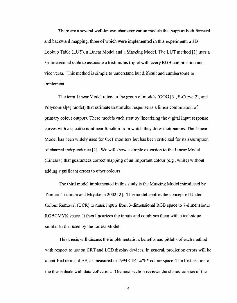
2.3 Device Characteristics
Seven devices were tested: two CRT monitors, three LCD monitors, and two LCD
projectors. A summary of these devices is given in Table 2- 1. One important issue in
characterizing a display is whether each channel's response is independent of the other
channels. In this study, channel interaction is calculated as follows.
In this equation, v represents the input value for the channel in question, a and b
are constant values for the other two channels, and L(r,g,b) represents the measured
luminance for a given digital input. The equations for CIGREEN and CIBLUE are similar.
This equation measures how much the luminance of a primary changes when the other
two channels are on. The overall interaction error for each device (Table 2-1) was
calculated as
Table 2-1: Device Summary
Name
CRTI
CRT2
LCD1
LCD2
LCD3
PRI
PR2
Description
Samsung Syncmaster 900NF
NEC Accusync 95F
IBM 9495
NEC 1700V
Samsung 171 N
Proxima LCD Desktop Projector 9250
Proxima LCD Ultralight LX
Interaction Mean
2.1%
1.5%
0.2%
2.2%
1.2%
0.2%
0.4%
Interaction Max
9.4%
4.9%
0.4%
4.1%
2.7%
0.5%
0.7%
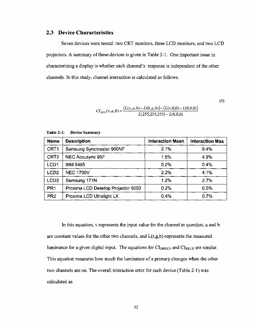
where N is the averaging factor = (XS+ 1 )*3.
From end-user point of view, three of the five LCD devices showed almost no
channel interaction; however, both CRT monitors exhibited significant channel
interaction (Figure 2-3). The interaction on the CRT monitors was generally subtractive
(leading to lower luminance) while on the LCD monitors it was either additive or
negligible.

Figure 2-3: Channel Interaction. The horizontal axis represents the input value v ranging from 0 to 255 and the vertical axis represents the value of the channel interaction metric, CICOLOR(v,a,b). The black Line shows a=b=255 and dashed lines show a=O,b=255 and
Red Green Blue
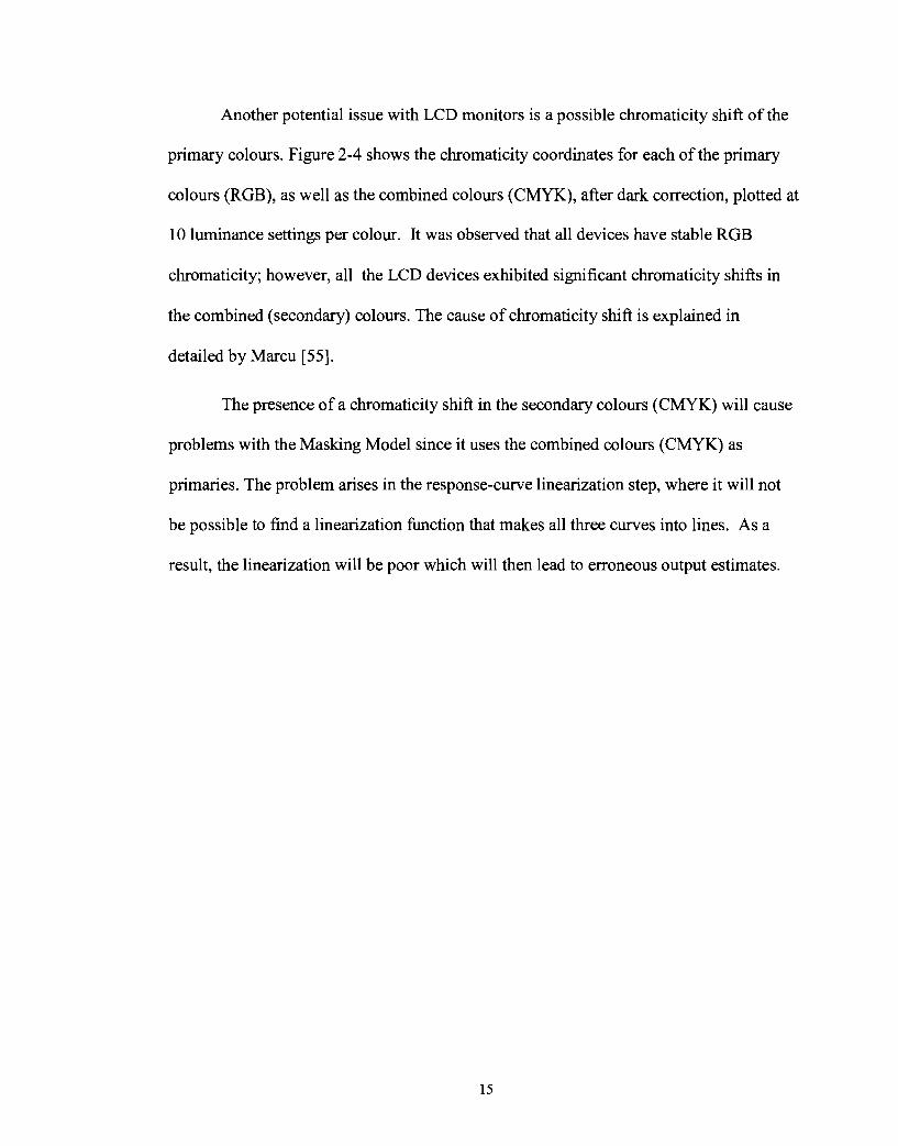
Another potential issue with LCD monitors is a possible chromaticity shift of the
primary colours. Figure 2-4 shows the chromaticity coordinates for each of the primary
colours (RGB), as well as the combined colours (CMYK), after dark correction, plotted at
10 luminance settings per colour. It was observed that all devices have stable RGB
chromaticity; however, all the LCD devices exhibited significant chromaticity shifts in
the combined (secondary) colours. The cause of chromaticity shift is explained in
detailed by Marcu [55] .
The presence of a chromaticity shift in the secondary colours (CMYK) will cause
problems with the Masking Model since it uses the combined colours (CMYK) as
primaries. The problem arises in the response-curve linearization step, where it will not
be possible to find a linearization function that makes all three curves into lines. As a
result, the linearization will be poor which will then lead to erroneous output estimates.

Figure 2-4 Chromaticity shift shown as intensity is increased plotted in xy space with x=X/(X+Y+Z) on the horizontal axis and y=Y/(X+Y+Z) on the vertical axis. When there is no chromaticity shift, all the dots of one colour lie on top of one another and therefore appear as a single dot.
CRTl

2.4 Implementation Details
All characterization methods start with black-level correction in which the measured
XYZ value of black (minimum output) for the device is subtracted fiom the measured
tristimulus value of each colour. This ensures that all devices have a common black point
of (0,0,0) in XYZ space. Fairchild et. al. discuss the importance of this step [50]. The
remaining steps for each characterization differ based on the method and are described
below.
2.4.1 3D LUT Model
The 3D LUT method was implemented with the intention of provic ding a standarc
against which to evaluate the other two models [I]. It is expensive both in time and space
(-10 MB for the lookup table) and is not well suited for reverse mapping. To create the
forward lookup table, the 1 Ox 1 Ox 10 training data is interpolated using 3D linear
interpolation to fill a 52x52~52 lookup table indexed by RGB values spaced 5 units apart.
At look-up time, 3D spline interpolation is used to look up intermediate values.
Inverting the lookup to index by XYZ requires interpolation of a sparse 3D data
set, which is non-trivial and an independent area of research [49]. The reverse lookup
was performed via tetrahedral interpolation into the original 10x1 0x1 0 data set.
Tetrahedral interpolation was chosen over a number of other methods primarily for its
speed and its ability to handle sparse, irregularly spaced data.
2.4.2 Linear Model
The Linear Model is a two-stage characterization process. In the first step, the raw
inputs di (i=l, 2, 3 for R, G, B) are linearized using a function Ci(di) fitted for each
channel. Linear regression is then used to determine the slope Mij between each
linearized input Ci(di) and the respective XYZ outputs where j=(l, 2, 3) for (X, Y, Z).
The second stage applies matrix M to calculate estimated XYZ values.
The LUT is calculated as follows. The 10 measured response values for the ith input
channel are interpolated to obtain three output vectors X(di), Y(di) and Z(di) in 256-
dimensional space. Principal component analysis is then used to find the single vector
Ci(di) that best approximates all three vectors. The following equation calculates Ci(di)
where PCAi represents the weighting vector obtained from principal component analysis
for channel i
In order to allow for backward mapping, two conditions are required: the
linearization function must be monotonic and the matrix M must be invertible. Inversion
is always possible because the input channels are linearly independent. However, the
monotonicity requirement is a real problem with LCD displays where the response curves
sometimes level out or even decline for high input values (Figure 2-5). It is therefore
necessary to modify the linearization function to ensure monotonicity as shown in Figure
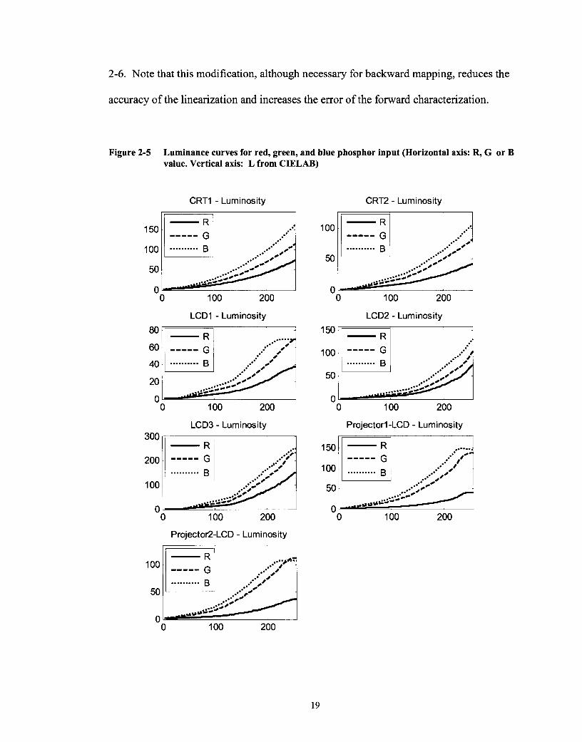
2-6. Note that this modification, although necessary for backward mapping, reduces the
accuracy of the linearization and increases the error of the forward characterization.
Figure 2-5 Luminance curves for red, green, and blue phosphor input (Horizontal axis: R, G or B value. Vertical axis: L from CIELAB)
CRTI - Luminosity
LCD1 - Luminosity
0 100 200
LCD3 - Luminosity 300 r , 1
Projector2-LCD - Luminosity I I I
CRT2 - Luminosity
rn f
LCD2 - Luminosity
m 1
Projector1 -LCD - Luminosity
0 100 200
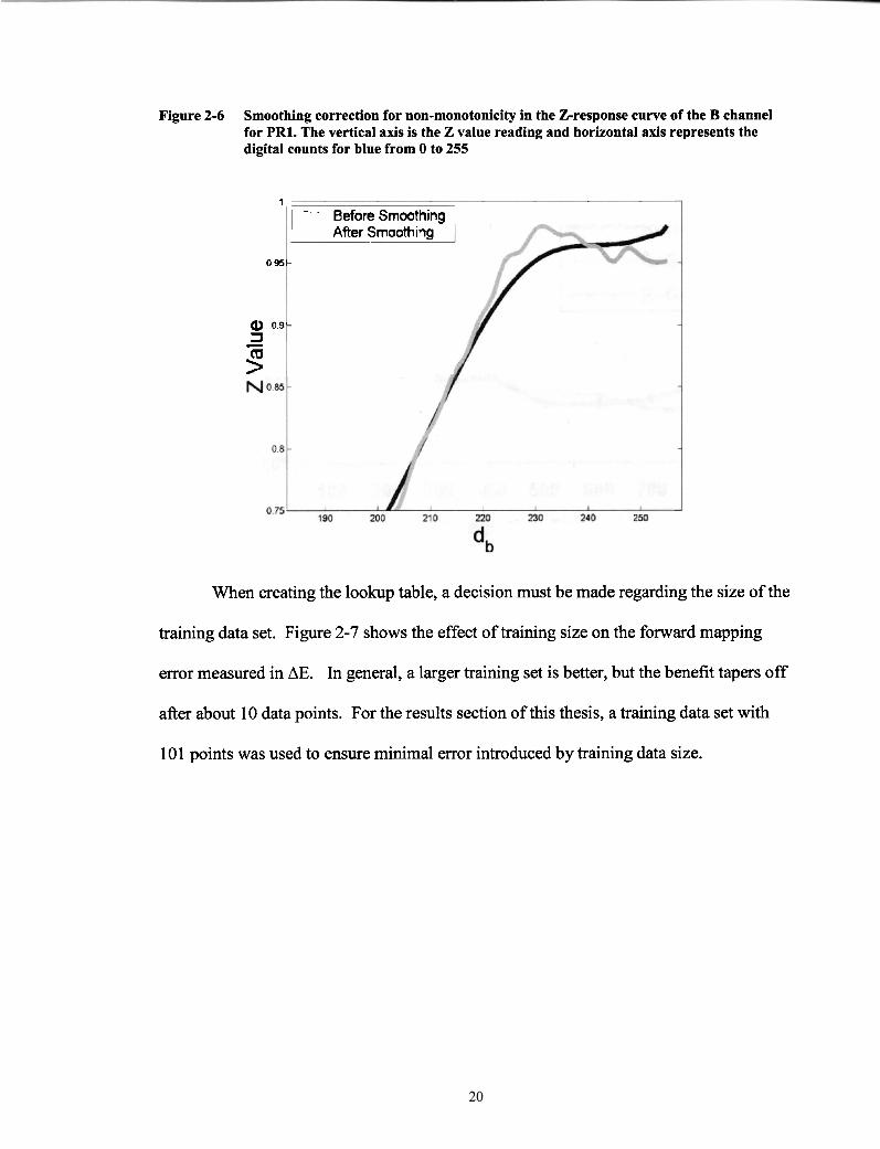
Figure 2-6 Smoothing correction for non-monotonicity in the Zresponse curve of the B channel for PR1. The vertical axis is the Z value reading and horizontal axis represents the digital counts for blue from 0 to 255
When creating the lookup table, a decision must be made regarding the size of the
training data set. Figure 2-7 shows the effect of training size on the forward mapping
error measured in AE. In general, a larger training set is better, but the benefit tapers off
after about 10 data points. For the results section of this thesis, a training data set with
101 points was used to ensure minimal error introduced by training data size.
1
095-
Q) 0 9 - 3 - P
- Before Smoothing After Smooth~ng 1

Figure 2-7 Mapping Error versus Training Data Size
Pebuv (LCD) - - AS Projector
The primary criticism of the Linear Model is that it assumes channel
independence. As we have seen above, this is not always a valid assumption - even for
CRT monitors. When there is channel interaction, the predicted output XYZ value for
colours that use more than one primary colour may not be accurate.
Predicting white and grey values correctly is crucial in colour calibration [51]. For
example, white is significant on computer-generated images such as presentation slides or
charts where there are large regions of pure white with no ambient lighting expected. We
observed that the Linear Model in general overestimates the luminance of white. There
are several approaches to addressing this issue. One technique , WPPPLS, imposes a
constraint so that the Linear Model emphasizes correct prediction of white [51].
A simple approach is to apply a diagonal transform to the slope matrix M based
on the measured and predicted values of pure white. The following formula shows the
conversion, where XMEASURED is the measured X value for white and XPRE~~CTED is the
predicted X value for white using the original slope matrix,.
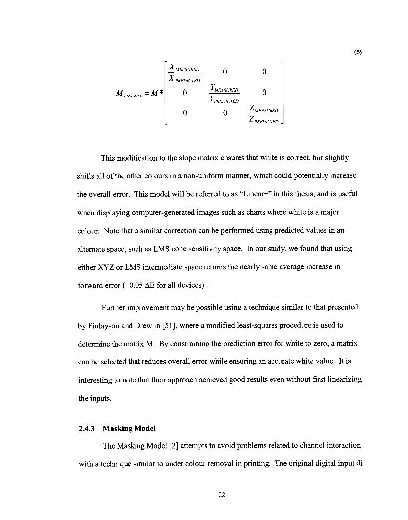
This modification to the slope matrix ensures that white is correct, but slightly
shifts all of the other colours in a non-uniform manner, which could potentially increase
the overall error. This model will be referred to as "Linear+" in this thesis, and is useful
when displaying computer-generated images such as charts where white is a major
colour. Note that a similar correction can be performed using predicted values in an
alternate space, such as LMS cone sensitivity space. In our study, we found that using
either XYZ or LMS intermediate space returns the nearly same average increase in
forward error (*0.05 AE for all devices) .
Further improvement may be possible using a technique similar to that presented
by Finlayson and Drew in [5 11, where a modified least-squares procedure is used to
determine the matrix M. By constraining the prediction error for white to zero, a matrix
can be selected that reduces overall error while ensuring an accurate white value. It is
interesting to note that their approach achieved good results even without first linearizing
the inputs.
2.4.3 Masking Model
The Masking Model [2] attempts to avoid problems related to channel interaction
with a technique similar to under colour removal in printing. The original digital input di
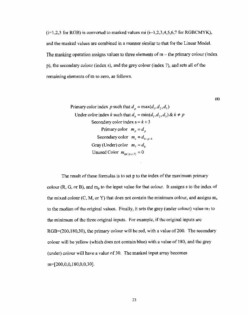
(i=1,2,3 for RGB) is converted to masked values mi (i=1,2,3,4,5,6,7 for RGBCMYK),
and the masked values are combined in a manner similar to that for the Linear Model.
The masking operation assigns values to three elements of m - the primary colour (index
p), the secondary colour (index s), and the grey colour (index 7), and sets all of the
remaining elements of m to zero, as follows.
Primary color index p such that d, = max(d, , d, , d, )
Under color index k such that d, = min(d, , d, , d,) & k # p
Secondary color index s = k + 3
Primary color m, = d,
Secondary color m, = d,-,-,
Gray (Under) color m, = d,
Unused Color m,,~p,s,7, = 0
The result of these formulas is to set p to the index of the maximum primary
colour (R, G, or B), and m, to the input value for that colour. It assigns s to the index of
the mixed colour (C, M, or Y) that does not contain the minimum colour, and assigns m,
to the median of the original values. Finally, it sets the grey (under colour) value m7 to
the minimum of the three original inputs. For example, if the original inputs are
RGB=(200,180,30), the primary colour will be red, with a value of 200. The secondary
colour will be yellow (which does not contain blue) with a value of 180, and the grey
(under) colour will have a value of 30. The masked input array becomes
m=[200,0,0,180,0,0,30].

Once the inputs have been converted into masked values mi, a linearization
function Ci(mi) for each input channel i is determined using the method described above
for the Linear Model. The slope matrix Mij for each input channel i and output channel j
is calculated as using PCA and linear regression, also as described for the Linear Model.
Finally, let the vector Pi represent the column of matrix M that contains the X, Y, and Z
slopes for input channel i. The transformation from masked input to XYZ output can
then be written as follows:
Here C,, C, and C7 represent the linearization functions for primary, secondary
and black component. The mi values are the values corresponding to each basis (primary,
secondary or black). The inverse mapping from XYZ to RGB is less obvious, and
requires knowledge of the primary and secondary colour indices p and s. There is no way
to know these values, so all six possible (p, s) combinations are tested (RM, RY, GC,
GY, BC, BM) and any combination that satisfies the following conditions will yield the
correct result.
2.5 Calibration Results
We calculated values of forward error AEFwD, round trip error AETRIP, and
backward error AEswD for 512 colours in an 8 x 8 ~ 8 evenly spaced grid of RGB inputs.
For each colour, we find three vertices in CIE L*a*b* space: the measured value for the
colour VM, the predicted value vp, and a round-trip value VRT. The round-trip value is
found by mapping backward and forward again fiom vp. These points form a triangle
with edges representing the forward, round-trip and backward error vectors. AEFWD is the
distance from VM to vp, AETR~P is the distance fiom vp to VRT, and AEswD is the distance
fiom VRT back to VM.
With respect to forward or backward error, we see that the 3D LUT is the most
accurate, followed by the Linear, Linear+ and Masking Models (Table 2-2, Table 2-3).
Note, however, that the Linear and Masking Models all have a round-trip error of zero,
while the 3D LUT has a non-zero round-trip error indicating an imperfect inversion. This
is not surprising considering the rounding error inherent in the sparse 3D interpolation
required to build the backward lookup table. The other interesting observation is that
Lin+ improved average forward error for CRTl which has higher CI than CRT2. This
data confirms that most of the error was due CI and a simple modification to the Linear
Model improves the overall performance.

Table 2-2 Forward mapping error: AE Mean (p ), standard deviation (a), and maximum.
I I LUT I Lin I Lin+ I Mask I
Average 1 0.8 1 5 6 ( 3.13 1 2.2 1 1.1 1 5.9 ( 2.5 1 1.3 1 6.8 1 4.0 1 2.1 1 10.3
CRTI
CRT2
LCD1
Table 2-3 Backward Error AE Mean (p), standard deviation (a), and maximum.
p
0.8
0.5
0.8
A comparison of backward error distributions (Figure 2-8) shows that the Linear
Model had the most compact distribution for each device, while the distribution for 3D
LUT tended to have a number of high-error outliers. The cause of these outliers becomes
PRI
PR2
Average
0
0.3
0.3
0.8
2.8
1.9
2.1
max
2.4
2.3
3.5
1.8
1.5
p
2.4
1.7
0.9
10.7
8.9
0
1.2
0.9
0.5
1.7
2.1
2.2
max
5.4
4.5
3.0
1.2
1.1
1.1
p
2.2
2.7
0.9
6.5
6.5
5.9
0
1.3
1.1
0.6
1.9
2.6
2.5
max
5.2
6.1
2.9
1.3
1.3
1.3
p
2.6
1.5
3.5
7.2
7.2
6.8
0
1.3
0.9
2.8
max
7.1
4.7
11.2
5.6
7.3
4.0
I
2.2
3.3
2.1
12.3
15.0
10.3

apparent when the error values are plotted by chromaticity (Figure 2-9). Observe that the
largest errors for the 3D LUT are often on or near the gamut boundary.
For the Linear Model, the highest errors are fairly well distributed across the
chromaticity space for all devices except the projectors, which have a distinct problem in
the blue region. This is most likely due to the non-monoticity exhibited by the projectors
in the blue output curves (Figure 2-5). As mentioned in the implementation section, the
monotonicity correction stage is a potential source of error for all devices. However, it
appears to be adding very little error for devices that do not have a monotonicity problem
(Table 2-4). The most notable increase in error was seen with the Projector 1, which also
had the most trouble with non-monotonicity.
Table 2-4 Percent Increase in Forward AE Error Due to Monotonicity Correction using Linear Model
I Uncorrected I Corrected [ % increase CRTl I 2.4 I 2.4 I 0.0%
Average I 2.2 I 2.2 I 2.3%
The average error for the Linear+ model was nearly the same as that for the
standard Linear Model. Recall that the goal of Linear+ is to guarantee that the predicted
white is correct, at the possible expense of other colours predictions. The results in Table
2-2 and Table 2-3 show little increase in overall error, which means a "perfect" white can

be achieved without much degradation in other colours. Informal visual comparisons
indicate that this model is often the best one to use for computer-generated graphics.
The Masking Model was expected to out-perform the Linear Model whenever
there was an issue with channel interaction. However, the model's best performance (on
CRT2) is only slightly better than that of the Linear Model. The primary pitfall of this
model is that it depends on constant-chromaticity "combined primaries" (CMYK). It is
clear from Figure 2-4 that this assumption fails for the LCD monitors and projectors. The
chromaticity shift causes the input the linearization step to fail. Figure 2- 10 shows an
example of an unsuccessful linearization for the black channel for PRl in the Masking
Model.
This explains why the performance of the Masking Model was better for the CRT
monitors than any of the other devices- the CRTs do not have the shifting chromaticity
problem. It is also interesting to note that on CRT2, the Linear+ algorithm introduced the
largest amount of error, indicating that the interaction present on this monitor is not well
suited for correction with non-uniform scaling.
With respect to efficiency, the Linear Model is the best. The Linear Model is
slightly faster than the Masking Model and nearly 20 times faster than the 3D LUT. The
Linear Model also requires less than half the storage space of the Masking Model, and
less than 11300th the storage space required for 3D LUT (Table 2-5).

2.6 Summary of the Calibration Study
Several display characterization models were implemented in this thesis: a 3D
LUT, a Linear Model, an extension to the Linear Model, and a Masking Model. These
characterization models were each tested on seven devices: two CRT Monitors, three
LCD monitors and two LCD projectors. The devices are characterized from and end user
perspective in which the devices are treated as black boxes with no knowledge or control
over their internal workings.
Table 2-5 Experimental cpu time and storage space relative to the time and space used by the Linear Model
In characterizing the devices, two issues that were of particular importance were
phosphor stabilization time and spectroradiometer integration time (Figure 2-1, Figure
2-2). We found that the phosphor stabilization time on the CRT monitors can take up to
10 seconds. In practice, a delay time of 2500 ms between colour display and
measurement resulted in acceptable error levels. With respect to integration time, we
propose that measurements on CRT monitors be taken with integration times that are
multiples of the display scan rate. In addition, we observed that a training set of 10 data
points per axis was sufficient for an accurate Linear Model for each of our 7 displays.
(Figure 2-7).
Linear
Masking
3D LUT
Although recent thesiss have indicated that the Linear Model is not applicable to
LCD panels [2], it worked well for the LCD display tested in this experiment.
Furthermore, the channel interaction problem was more pronounced on the CRT monitors
Time
1 .O
1.2
17.0
Space
1 .O
2.3
333.4

than on several of the LCD displays. The fact that we did not find channel interaction
with the LCD's we tested does not mean that it is not present in LCD panels themselves.
We tested completed LCD displays which include electronics specifically designed to
mitigate the effects of channel interaction. Nonetheless, from an end-user point of view,
channel interaction did not pose a problem. The primary issue with the LCD displays was
the fact that the response curves for the three input channels were dissimilar, leading to
chromaticity shift of combined colours (CMYK). This problem affected the Masking
Model but not the Linear Model.
Despite these issues of linearization and channel interaction, all three models
yielded a level of error that on average has a mean of less than 4 AE and a worst case less
than 15 AE. The 3D LUT model was slightly more accurate than the other models, but it
is too cumbersome for actual use. The Linear Model was the most efficient, with
accuracy nearly as good as to the 3D LUT. The primary drawback of the Linear Model is
that it can be adversely affected by channel interaction. A slight modification to the
Linear Model is presented in the Linear+ model that uses a simple white-point correction
technique to ensure correct prediction of white. Our results indicate the Linear+ model is
able to guarantee white-point accuracy with minimal degradation for other colours.
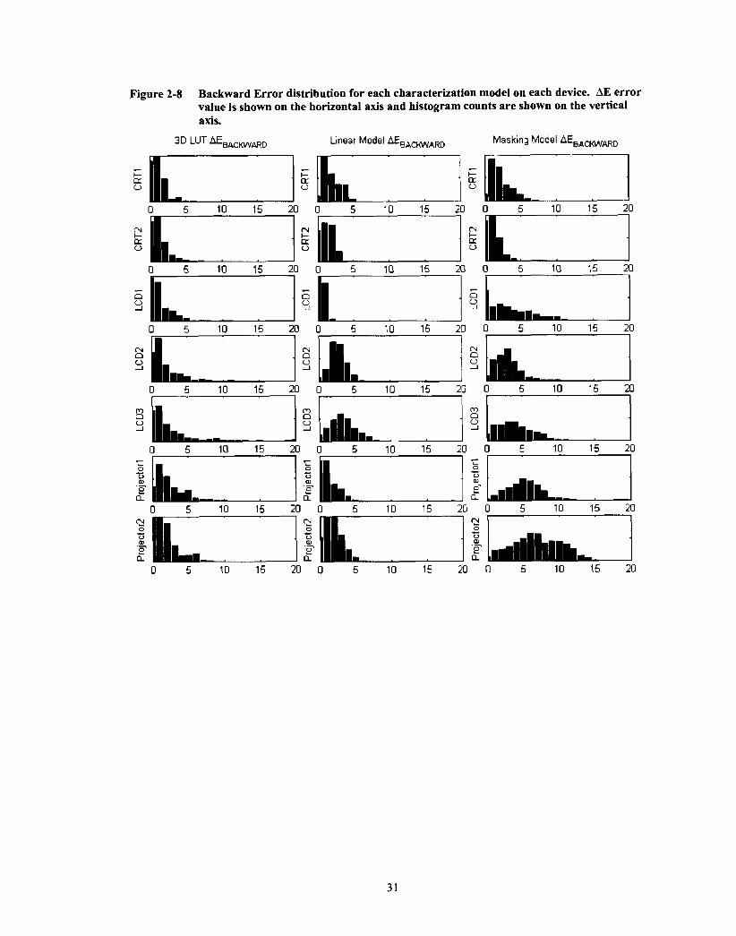
Figure 2-8 Backward Error distribution for each characterization model on each device. AE error value is shown on the horizontal axis and histogram counts are shown on the vertical axis.
Linear Model AEBACKWARD Masking Model AEBACWARD

Figure 2-9 Comparison of Outliers for the Backward model. Vertical axis and horizontd axes represent YJ(X+Y+Z) and M/(X+Y+Z) respectively. The AE error is plotted according to the legend of grey scales. The circular points represent outliers with AE greater than 1.5 times the average error. The majority of the high outlier errors for LUT model occur near the gamut boundaries.. The outliers for Linear Model are quite negligible compared to the other two models.
3D LUT Linear Model Masking Model

Figure 2-10 Linearization failure for the black channel on PR1
0.2 0.4 0.6 0.8 1
Linearized M Channel Input

CHAPTER 3: OPTIMAL DEVICE CALIBRATION
3.1 Introduction
In this section, we try to study whether the traditional Device Calibration used for
electronic display can be improved. As was explained earlier, a forward Linear Model is
based on a 3-by-3 linear transformation matrix M mapping data from (linearized) RGB to
XYZ. A typical approach for generating the matrix M is by applying least squares
between linearized RGB and measured XYZ [5 11 or using principal component analysis
(Section 2.4.2). Although these two methods for calculating M work well, they both
suffer from the fact that they try to minimize error in XYZ space, which is perceptually
non-uniform.
In this chapter we propose two methods for calculating M which is based on more
directly optimizing the error measure in CIELAB. The first approach (LabLS) extends
the least-square model (ULS) by applying weights to the model. Weights represent
importance of a colour in CIELAB space (the space that is important to us).
The second method is based on optimizing the AE error directly using the Nelder-
Mead simplex algorithm [56]. Unfortunately, the Nelder-Mead algorithm (not to be
confused with the linear programming simplex algorithm) finds a local minimum and
does not guarantee a globally optimal solution. However, by using the results of the
LabLS method as the starting condition, we have found experimentally that it converges
reliably to excellent solutions. This method will be referred to as DEM since it is based
on a AEg4 minimization.
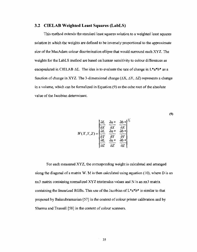
3.2 CIELAB Weighted Least Squares (LabLS)
This method extends the standard least squares solution to a weighted least squares
solution in which the weights are defined to be inversely proportional to the approximate
size of the MacAdam colour discrimination ellipse that would surround each XYZ. The
weights for the LabLS method are based on human sensitivity to colour differences as
encapsulated in CIELAB AE. The idea is to evaluate the rate of change in L*a*b* as a
h c t i o n of change in XYZ. The 3-dimensional change (AX, AY, AZ) represents a change
in a volume, which can be formalized in Equation (9) as the cube root of the absolute
value of the Jacobian determinant.
For each measured XYZ, the corresponding weight is calculated and arranged
along the diagonal of a matrix W. M is then calculated using equation (lo), where D is an
11x3 matrix containing normalized XYZ tristimulus values and N is an 11x3 matrix
containing the linearized RGBs. This use of the Jacobian of L*a*b* is similar to that
proposed by Balasubrarnanian [57] in the context of colour printer calibration and by
Sharma and Trussell [58] in the context of colour scanners.

3.3 AE Minimization (DEM)
Nedler-Mead simplex [56] search is a directed search method for multi-
dimensional non-linear regression. This search can be used to optimize the 9 parameters
in matrix M so that the calibration error is minimized. In this thesis we used the Matlab
function fininserach to find the 9 values in matrix M, however any local-search algorithm
can be used.
The solution depends on the starting conditions. It is shown below that the
Nedler-Mead simplex search outperforms other models when it starts with an initial
solution found by LabLS.
3.4 Measurement Characteristics
We used the measurements for the 7 displays mentioned in Table 2-1 that was
originally used to compare Linear Model and Masking Model performance.
Similarly, all three RGB channels are linearized respect to XYZ values.
3.5 Results
The ULS, LabLS and DEM methods of computing the RGB-to-XYZ
transformation matrix, M, were applied to the same 1000 measured colours as in Chapter
2. All these values are used after they are linearized and normalized with respect to the
white of the display. In each case, the resulting M is evaluated by using it to map the
1000 RGB inputs to XYZ and measuring the difference between the predicted and
measured values. The difference is calculated in terms of the average AE94 error
measures.
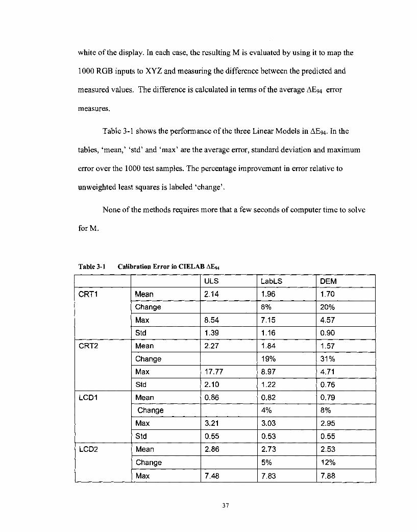
Table 3-1 shows the performance of the three Linear Models in AE94. In the
tables, 'mean,' 'std' and 'max' are the average error, standard deviation and maximum
error over the 1000 test samples. The percentage improvement in error relative to
unweighted least squares is labeled 'change'.
None of the methods requires more that a few seconds of computer time to solve
for M.
Table 3-1 Calibration Error in CIELAB AEg4

Mean 1 3.65 1 3.28 1 3.10 I Std
Change I 1 10% 1 15% I
ULS
1.44
Std 1 1.26 1 1.27 1 1.55 I
Max
Std
Mean
Change
Mean 1 1.98 1 1.91 1 1.88 I
LabLS
1.41
Change I 1 4% 1 5% I
DEM
1.39
7.25
1.43
1.73
Max 1 6.29 1 7.91 1 9.11 I
8.42
1.44
1.54
11%
Comparing Table 3-1 with Table 2-2 shows that there is no advantage between
9.45
1.67
1.46
16%
Std
calculating the matrix M using Least Squares (ULS) or using coefficient of PCA (Section
2.4.2), and both LabLS and DEM have improvements over the old two methods.
1.13 1 1.16
3.6 Summary of Optimal Device Calibration
The performance of a 3x3 linear colour calibration model can be improved by optimizing
for the transformation matrix in spaces other than XYZ. One alternative (DEM) is to
minimize directly in CIELAB space, but this involves nonlinear optimization. Another
alternative (LabLS) is to optimize using weighted least squares regression in a CIELAB-
weighted version of XYZ. Experiments in calibrating with 7 different displays show that
both methods significantly reduce calibration errors as measured in terms of average and
maximum AE94 error.
1.27

CHAPTER 4: GAMUT MAPPING FOR ELECTRONIC DISPLAYS
4.1 Gamut Mapping Introduction
A gamut is the range of colours that can be formed by all combinations of a given
set of light sources or colourants of a colour reproduction system. The human eye can
perceive a wide gamut of colours within the full range of the visible spectrum, including
detail in very bright light and deep shadows. Reflected light, ink impurities, and paper
absorption, all limit a conventionally printed image colour gamut [I 11. Similar effect
happen on monitors and projectors as each display can produce a limited range of
colours. Similarly, we can define a gamut for an image, which is the set of all the colours
found in it. In this thesis, we focus on the gamut of electronic display and more
specifically on the CRT and LCD displays.
In order to be able to preview one display's output on another display, we need to
find a way to overcome the difference between gamuts of displays. The source gamut is
the gamut of a display or an image that is desired to be mapped. The target gamut, on the
other hand, is the gamut of the display that the image is intended to be viewed on. The
Gamut Mapping Algorithm (GMA) try to find a mapping between the two gamuts. A
GMA should allow for different rendering intents (e.g. accuracy, pleasant, retinex
reproduction).
Most GMAs are based on the assumption that the design of the optimal technique
involves combination of image attributes such as contrast, luminance detail, vividness,

and smoothness. The followings are the general measurement factors and goals for a
GMA identified by Jan Morovic [ 131 and MacDonald [ 151.
Preserve the Grey Axis of the image for maximum luminance contrast.
Minimize the hue shift. Most of the display-based GMAs are designed to
preserve the hue angle by allowing changes in saturation or luminance.
Increase in saturation is preferred. Even though the saturation might be
limited after the gamuts are mapped, at least the available potential
saturations should be used.
There are two general gamut mapping algorithms [7 ] . The first category is solely
device dependent, where gamut mapping is a fimction of input and output device gamut
and the algorithm is independent of image content. The majority of gamut mapping
algorithms fall in this category [13]. In this approach, the gamut mapping is a point-wise
operation from an input point to an output point in an appropriate (usually perceptual) 3D
colour space. One of the fundamental problems with such point-wise operation is that it
does not take important spatial neighbourhood effects in an image into account. We refer
to this type of GMA as device-based GMA.
The second category of gamut mapping algorithms, content-based GMA,
considers spatial characteristics in addition to colour characteristics of the image. Using
these algorithms, two pixels of the same colour in an image can map to different colours
in the output image, depending on the spatial characteristics in the neighbourhood of the
pixels.
The majority of the study on GMAs is between monitors and printers that have a
very different gamut shape. In this thesis, we specifically focus on gamut mapping
between electronic displays. We show improvements that we can make to existing GMAs
by considering common characteristics between gamut of electronic displays.
This section starts by studying the properties of LCD and CRT gamuts. Methods
for determining gamut boundary and finding OOG are explained. The next part starts
with a detailed introduction to different types of device-based GMA. We introduce an
algorithm for fitting most of the source gamut inside the target gamut before any device-
based mapping is applied to bring the remaining OOG colours inside gamut. This
algorithms is based on the similar shape of the gamut of displays and tries to preserve the
hue angle for each colour. At the end, performance of this new algorithm is compared to
other existing algorithms, including some content-based GMAs that take longer CPU
time.
4.2 Characteristics of LCD and CRT Display Gamut
4.2.1 Gamut Shape
Electronic displays such as LCD and CRT displays have an additive gamut
compared to a printer's gamut which has a subtractive gamut. Additive means that their
gamuts are created by adding lights; whereas for printers, the gamut is created by
reducing reflectance light from the paper. In Color.org [14] website there is a visual
comparison between CRT monitor gamut shape and a 4-ink inkjet printer. It is obvious
that these two devices, monitor and printer, have different shape, one is quite convex and
the other one has concavities in multiple places.

Out of 7 displays shown in Table 2-1 that we studied in this thesis, we observed
that all of them have a convex shape gamut with very similar shape. In general, it is
expected that these devices will have a convex gamut since their colour space is
generated in an additive form by combining three different lights (R, G, B). Figure 4-1
and Figure 4-2 show 1500 colours measured inside each of these gamuts in XYZ and
CIELAB colour space.

Figure 4-1 Gamut shape of Displays in XYZ space
C RTI

Figure 4-2 Gamut shape of displays in L*a*b* space
CRTl CRT'2 ,..'I.._ . . . . . ::. _ . . . . . . . . . . . . . . . . . . . . . . . . . . . ..... . . . .
joo-.." : . . . .
.... .... * .: -P
' . _ .. . I : . . . 100 100
a* -100 0 L* a* - 1 0 0 0 L*

From these two figures we can see that all the devices that we tested have a
convex gamut shape. In this thesis we try to take advantage of this property of display
gamut for mapping colours and predicting the gamut boundary.
4.2.2 Predicting Out of Gamut
Predicting the gamut boundary, and as a result finding OOGs, is quite challenging
when a gamut is concave. However, as it was shown earlier, we can assume that LCD
and CRT gamuts are convex. Knowing this property simplifies the prediction of the
gamut boundary and finding OOGs. The simplest approach to calculate a convex surface
is by finding the convex hull of the set of given points, in this case measured XYZ or
L*a*b* values. The convex hull of a data set in n-dimensional space is defined as the
smallest convex region that contains the data set [2 11. In our case, since we are working
with a three-dimensional data-set (XYZ or L*a*b*), the facets that make up the convex
hull are triangles.
References [22] and [23] have detailed information on the convex-hull algorithm.
In this thesis we use a convex-hull implementation provided by Matlab.
4.2.3 Using Convex-Hull Algorithm to Predict Gamut Boundary
We can tessellate the surface of convex hull into triangles. Each triangle
represents a plane in 3D colour space. A plane in a 3-dimensional space is represented by
aX + bY + cZ - K = 0'. Now if we substitute a point (Xo, YO, Zo) into the formula, three
things can happen. The equation aXo + bYo + cZo - K can equal to zero meaning the
' Similar situation applies to L*a*b* values in CIELAB colour space.
point is on the plane. If the point is outside the plane, then the equation will be less or
greater than zero, depending on which side of the plane the point is.
This simple idea can be used to find whether a point, PA is outside the hull. If the
sign of one of the plane equations for convex hull boundary evaluated at a point, PA, is
different than the sign of the same plane evaluated on a point inside gamut, Pf, then the
PA is out of gamut.
If we have N triangles, and thus N plane equations, the time complexity of this
algorithm to find out if a colour is inlout of gamut is O(N). In general for the displays in
this thesis, we only needed under 250 triangles to represent the gamut surface. This
means that the algorithm can be quite fast.
4.3 Known Device-dependant GMAs
Device-dependant GMAs clip out OOG on or inside the target gamut boundary.
Their difference lies in how and where these points are clipped and whether inside-gamut
colours are changed. Sometimes, there is more than one name refemng to the same GMA
and for clarity, we use the terms introduced by CIE [14].
In this section, we start by looking at different methods of mapping. We introduce
an extension to the clipping algorithms and in the next section, we compare the
performance of all the device-based mapping. Evaluating GMA performance requires
visual comparison and for this thesis we did not run a human study. The models were
evaluated by the graduate student, Behnam Bastani. In most cases the difference is quite
noticeable. Some of the images are provided later in this section for the reader.
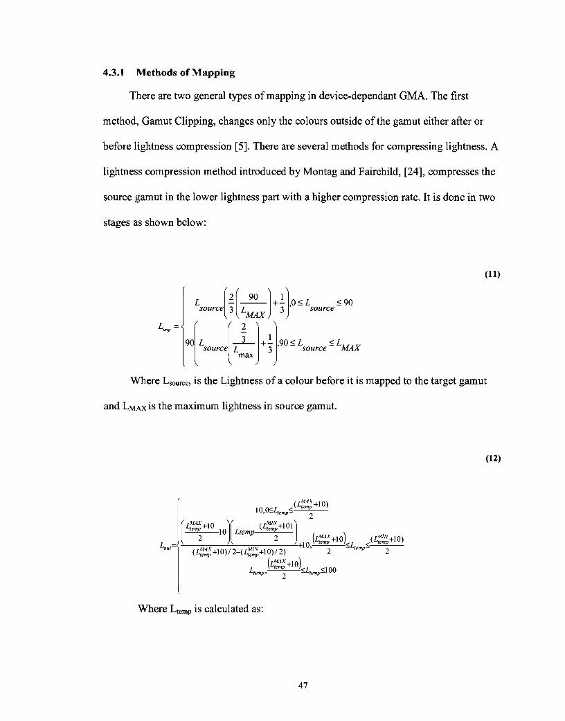
4.3.1 Methods of Mapping
There are two general types of mapping in device-dependant GMA. The first
method, Gamut Clipping, changes only the colours outside of the gamut either after or
before lightness compression [5]. There are several methods for compressing lightness. A
lightness compression method introduced by Montag and Fairchild, [24], compresses the
source gamut in the lower lightness part with a higher compression rate. It is done in two
stages as shown below:
Where L,,,,, is the Lightness of a colour before it is mapped to the target gamut
and LMAX is the maximum lightness in source gamut.
Where L,,,, is calculated as:

Lo,, is the original colour mapped to the target gamut. In this thesis we use a
gamma shape compression for lightness which results in an output image that has a
smoother lightness than the above piece-wise linear compression method.
After lightness adjustment, clipping methods clip the Chroma of colours that are
outside of the target gamuts in three general directions until the colour is on the target
gamut surface. One major drawback of clipping methods is that while they maintain most
of the image saturation, clipping can cuase loss of gradation in an image because some of
the colours are mapped to the same point [ 2 5 ] .
Gamut Compression is the second approach for device-dependant GMAs which
changes all the colours in source gamut. It compresses the source gamut until most of its
colours fit inside target gamut space. This method is mainly used when there is a big
difference between the two gamuts (e.g. monitor and printer gamuts). There are 3 general
compression methods:
Linear compression: All the colours, including inside gamut colours are
scaled so that all the data are within the target gamut. This method
maintains the gradations in the image, but it can sometimes cause an
objectionable decrease in saturation.
Non-linear compression: This algorithm applies a polynomial function for
scaling the colours. This method tries to compress the colours closer to the

source gamut boundary with a larger factor [26] . By compressing some of
the inside gamut colours, this method reduces the loss in saturation while it
retains the advantage of reproducing accurately most of the common gamut
colours [B].
Piece-wise linear compression: Non-linear compression is slow to
implement since every colour compresses differently. Piece-wise linear
compression tries to mimic non-linear behaviour by breaking the target
gamut into different layers. Colours in the gamut have a different linear
compression depending on which layer of target gamut they fall into.
In general, if source and target gamuts are similar the preferred technique is the
clipping method. If the number of OOGs is large, a linear or non-linear compression is
preferred. Figure 4-3 compares behaviour of the above methods.
Figure 4-3 Gamut clipping and compression along a given direction. Target represent Target Gamut boundary and Source is the source (original) gamut boundary [13]

Some techniques design a different non-linear compression method depending on
image contents. For instance, if the saturated OOGs contain high frequency components,
a different degree of compression is used compared to when those colours only have
gradual change with low frequency components [25]. This is the motivation for having
image-based (content-based) gamut mapping. Nakauchi et a1 [27] proposed a technique
that improves the display-based mappings by applying a spatial convolution filter to an
image. This technique is later improved by Kimmel et a1 [8] which will be discussed in
Content Based Gamut Mapping section.
4.3.2 Direction of Mapping
When the type of clipping is set, the next step is to decide in what direction the
mapping should be applied. There are three general directions that are mainly used in the
literature [5], [13]:
Straight Direction: The chroma of a colour is reduced by keeping its hue
and lightness constant until the colours lies on the target gamut surface.
Node Direction: The chroma is clipped towards a single centre-of-gravity.
The most common centre-of-gravity is lightness = 50. Colours are clipped
in the direction towards lightness = 50 while keeping hue constant.
Cusp Direction: The lightness and chroma of a colour are changed towards
lightness of maximum chroma (cusp) in a given hue angle.
Figure 4-4 shows Straight, Node and Cusp directions for mapping.

Figure 4-4 Directions for gamut-mapping
Figure 4-5, Figure 4-6 and Figure 4-7 show the behaviour of colour gamut with
hue angle =lo-20 degrees for the Straight, Node and Cusp clipping from CRTl as the
source gamut onto LCD1 as the target gamut. The blue arrows show the direction of
mapping and green dots represents the colour gamut data after mapping to target gamut
space. Colours that are already inside target gamut do not move.
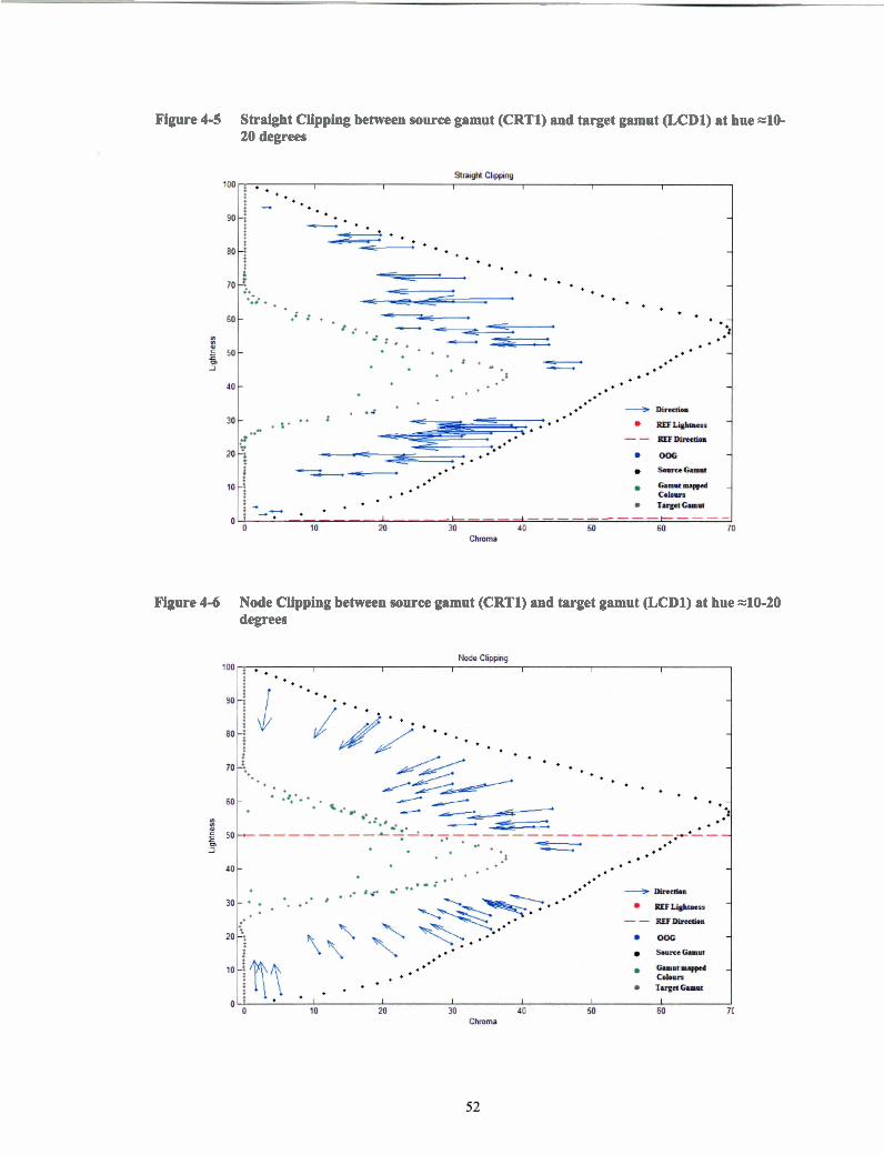
Figure 4-5 Straight Clipping between source gamut (CRTl) and target gamut (LCD1) at hue ~ 1 0 - 20 degrees
Figure 4-6 Node Clipping between source gamut (CRTl) and target gamut (LCD1) at hue 40-20 degrees
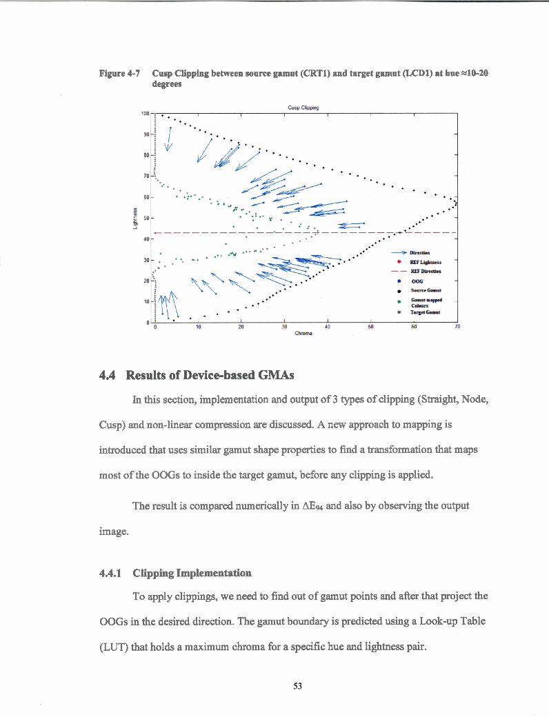
Figure 4-7 Cusp Clipping between source gamut (CRT1) and target gamut (LCD1) at hue =lo-20 degrees
4.4 Results of Devicebased GMAs
In this section, implementation and output of 3 types of clipping (Straight, Node,
Cusp) and non-linear compression are discussed. A new approach to mapping is
introduced that uses similar gamut shape properties to find a transformation that maps
most of the OOGs to inside the target gamut, before any clipping is applied.
The result is compared numerically in AEg4 and also by observing the output
image.
4.4.1 Clipping Implementation
To apply clippings, we need to find out of gamut points and after that project the
OOGs in the desired direction. The gamut boundary is predicted using a Look-up Table
(LUT) that holds a maximum chroma for a specific hue and lightness pair.
To clip a colour, its hue angle and lightness is used to grab the proper LUT. This
LUT is calculated ahead of time using Convex hull idea explained earlier. Depending on
the direction of mapping, we grab the desired maximum chroma from LUT. Table 4-1
compares the results of the three different mapping directions in AEg4 on 1000 colours
between CRT 1 as source gamut and LCD 1 as target gamut.
Table 4-1: Clipping comparison in AECIECAMOZ. 1000 colours were used CRTl (source gamut) and LCD1 (target gamut)
This table shows that all three directions have similar numerical results. However,
visibly comparing Straight clipping versus the other two clipping algorithms shows that
Straight clipping preserves contrast of the image better than the other two mappings, and
it has more desirable outputs than the other two GMA.
Max AEg4
Mean AEg4
4.4.2 Non-linear Compression Mapping, Implementation
Compression mapping is more time complex than general clipping methods. In
this mapping algorithm, generally one or more polynomial functions are introduced to
map colours from source gamut to the target. More precisely, in Clipping methods, only
the outside gamut colours would get mapped and the remaining colours stay unchanged.
Non-linear compression not only forces the OOG colours to map on or inside the target
gamut, but also forces the colours inside gamut to move as well. The idea is to preserve
some of the contrast that might have been lost because of clipping only OOG colours.
Straight Clipping
15.8
5.7
Node Clipping
21.9
5.4
Cusp Clipping
18.8
5.9

In this mapping algorithm, we need to define a mapping between some reference
colours between source and target gamut. Other colours are mapped using an
interpolation. We use 3D spline interpolation to calculate mapped colours. Spline is used
mainly because it can result in a smoother output image.
There are several options for selecting the pivots (reference colours). One
approach is to map the colours between displays using their naming in digital values
(RGB). For instance, a maximum yellow in DeviceA and Devicee can be defined as
tristimulus values corresponding to R=255,G=255,B=O. The benefit of using this
approach is that we have many more variables to work with and optimally we have a
better precision in mapping two devices' gamuts. The major drawback is that due to non-
similarity of relation between digital inputs and tristimulus value it is quite possible that
full yellow has tristimulus values smaller than a yellow colour with lower R and G
values. This issue was discussed in more detail in Section 2.3.
The other choice is to use corners of a device gamut in CIELAB space to
represent a colour. Looking at the Figure 4-8 we can see that some specific colours are
obvious. The two colours that have similar representations in all 7 displays are maximum
blue and green inside each gamut. Maximum blue can be defined as a colour with the
lowest b* and a* that has largest L* values in CIELAB. Similarly the maximum green
colour is the colour inside each gamut with the highest L* and b* values and lowest a*.
Other colours such as maximum red are much harder to be defined accurately. The main
drawback of this approach is not having enough reference points to use for mapping.
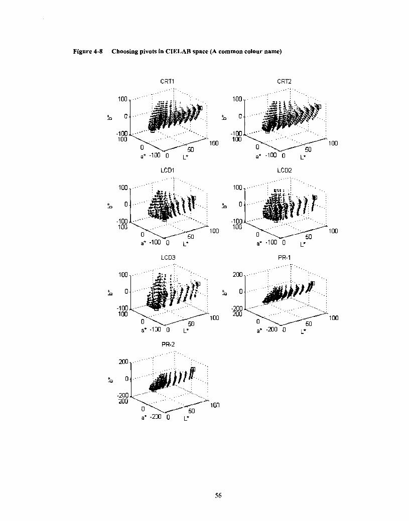
Figure 4-8 Choosing pivots in CIELAB space (A common colour name)

The next approach is to look at each hue slice and use the cusp of each hue slice
as a reference colour (pivot). All devices including printers, monitors and projectors are
known to have a cusp when looking at hue slice that has around 10 degrees range. Figure
4-9 shows the gamut of CRTl for hue slice between 10-20 degrees. To find cusps
accurately, the gamut space needs to be sampled in detail. We used the Linear Model to
populate the gamut and looked at each hue slice to find the cusps. To preserve grey axis,
grey colour (X=Y=Z in XYZ space) is added to the list of reference colours.
Figure 4-9 Scatter of colours in a hue slice. The cusp (colour with maximum chroma) is the. point with largest chroma value. Horizontal and vertical axis represent chroma and lightness.
CRTl
& o b 60 70 80 90 l o o 110 Chroma
Once pivots are chosen, a 3D spline interpolation is applied to interpolate any
other colours respect to the pivot points. After interpolation, it is possible to have some
colours left outside the target gamut. Straight clipping is done to bring the remaining

OOGs inside the target gamut. Table 4-2 shows the numerical result of this non-linear
method.
Table 4-2 Effect of non-linear compression on gamut mapping between source gamut (CRT1) and target gamut (LCD1). This data is based on 1000 measured colour for each gamut. The change in gamut mapped colours is measured in AE
/ Mean AE
A drawback of non-linear compression is that the quality of the model depends on
so many variables, including type of compression and choice of reference colours used.
These settings may need to be different depending on the image gamut [13].
The major problem with non-linear compression is that it requires more CPU time
to operate. This GMA generally take longer CPU time than clipping methods, which
makes it a non-feasible approach for applications that require real-time mapping.
4.4.3 Combination of Linear Transformation and Clipping
Looking at Figure 4-2 shows that CRT and LCD displays both have similar gamut
shape. In this section, we show that transforming the source gamut linearly to fit on the
target gamut can improve the quality of the image significantly. This mapping algorithm
takes advantage of the non-linear compression algorithm but uses less CPU time overall.
Reference colours are chosen as discussed in 4.4.2 and least-squares is used to find the
best mapping between the source and target gamut. Straight clipping is used on the
remaining OOGs similar to the last step of the non-linear compression. We refer to this
GMA as TS-Clipping (Transformed+Straight Clipping).
Table 4-3 Difference between colours after TS-clipping is applied and before that. This data is based on 1000 measured colour for each gamut. The change in gamut mapped colours is measured in AE
Figure 4-10 and Figure 4-1 1 are the result of straight clipping and transformation
applied before straight clipping. These figures are provided for a general judgment. For
formal evaluation, we used the exact environment setting with two monitors beside each
other. Figure 4- 10 shows that the child face has lost reasonable contrast whereas TS-
Clipping in Figure 4-1 1 was able to preserve the overall contrast in the image.
TS-Clipping
Visual comparison of the above GMAs showed us that TS-clipping has a better
visual output than the other device-based GMA. Another advantage of this algorithm is
that after transformation, there are fewer OOGs lefi and as a result the Straight Clipping
part of the model is faster.
Mean AE
7.1
Max AE
2 1

Figure 4-10 Straight Clipping Result between source gamut (CRT1) and target gamut (LCD1)

Figure 4-11 Transformation applied before clipping. Result is between source gamut (CRT1) and target gamut (LCD1)
.; .:
4.5 Content Based Gamut Mapping , , . Most of the classical gaput mapping methods involve a pixel by pixel mapping,
devicedependent r I mapping. These methods ignore the spatial characteristics of images. In , , f ,- . ., 8 ' , , , --7
this section, we analyze two major algorithms to address this issue. These models are
computationally more complex and their performance greatly depends on input image
content.
Since it is hard to compare the performance of content-based models numerically,
we include output images. Test images are evaluated in two different methods. One set of

test cases is designed by constraining a display gamut in sRGB space. sRGB is used as
RGB so that results are independent of device characteristics and we can evaluate the
output on any display. The sRGB channels are restricted to [5O, 1501 range in this thesis
unless specified otherwise. Figure 4-12 shows effect of constraining gamut on an image.
Figure 4-12 Image gamut in CIELAB when its RGB channels are is the original gamut and red is the projected gamut.
restricted
-
range. Blue
The drawback of this model is that the gamut is built artificially and some of the
characteristics of the gamut of the displays might be lost.
For accuracy, these models are evaluated again using two monitors gamuts. The
main advantage of using the artificial gamuts is that these gamuts allow us to compared
the performance of the models in cases where the gamuts are significantly different from
each other.

4.5.1 Gamut Mapping to Preserve Spatial Luminance Variations: Bala [7]
The intuition behind this model is to recover the loss in luminance contrast after a
GMA is applied. The main use of this model is in computer-generated images. Computer
generated images are characterstized as being mainly a combination of very smooth
patterns and some sharp edges. An example that Bala's model can be used is for an image
on a CRT monitor that has black text on a blue background. The text is easily
distinguished against the background. However, if out-of-gamut colours were clipped on
the target display (on the gamut of the display used for previewing), the gamut at darker
colour becomes narrower than it should be. Applying Straight clipping results in CRT
blue being mapped to a much darker blue in the output device. As a result, much of the
luminance distinction is lost between text and background.
The general algorithm has three main parts. The first step applies a straight
compression mapping (typically straight clipping) that preserves Lightness and Hue. Next
the luminance of a pixel is adjusted if the luminance loss in one pixel is much greater
than the neighbouring pixels. In this algorithm, luminance refers to the Y component of
XYZ space.
The last section looks at the adjusted colours and if they are not in gamut, they are
clipped. However, this time the emphasize is not to preserve lightness. Figure 4-1 3 shows
the general structure of this mapping.

Figure 4-13 General structure of Luminance-Preserving Gamut Mapping, Adapted from [7]
4.5.1.1 Bala Algorithm, in Detail
The overall performance of this algorithm depends on the filter type and the final
GMA. The extent and spatial footprint of the enhancement depends directly on the
characteristics of the high-pass filter F. Bala uses the following simple linear filter:
Where S is the NxN neighbourhood around pixeli. The filter size, N, plays an
important role in the final output and its optimal size depends on the type of image. For
images with soft or noisy edges, e.g. scene image or scanned images, a large filter size is
required. Images that have sharp edges and relatively low noise, e.g. computer generated
images, need a smaller filter size. We should note that applying a large filter size to
images with sharp edges can cause halo effects.
Bala uses a simple approach for choosing the filter size. Filters have two types:
large area and small area filters with N=15 and N=3 respectively. For each region the
difference in Y between a pixel and its close neighbours is calculated (N=3), if the
difference is high, a small area filter is used. Otherwise, it is either a smooth plain pattern
or scanned pictorial image. A second difference is calculated, this time considering more
neighbouring pixels (N=15). If the difference is high, compared to smaller area
difference, a large area filter is used; otherwise, the image is like a smooth plain pattern
and small (N=3) area filter is required.
However, we should mention that the two filter sizes are generalized for the
printer gamut on plain thesis. For monitors we found that images such as scenes with
smooth but many edges required a filter size of Nz20. Computer generated images are
categorized into two parts. Text images, where multiple sharp edges are present and
graphs with few sharp edges on a plain and a very smooth background.
Text is a special case where we need to have good resolution in the horizontal
direction to differentiate between letters while there are normally larger gaps between
text lines. Therefore, text requires very small filter size on horizontal direction (N=3) and
large size for vertical direction (N=9). With text, we are specifically talking about text in
a document. Text for a document title that has a relatively larger font is categorized as
second type of computer generated images (graphs). Graphs are treated differently and
use a square shape filter of size (N=3).
4.5.1.2 Bala's Algorithm Results
Scene images such as the one in Figure 4- 14 require a much more flexible filter to
hl ly recover edges and not add noise. We observed that Bala's model does not improve
the final result of a Straight Clipping and in some cases it even reduces the quality of
images that have detailed edges but most of them are smooth transitions.

Figure 4-14 A sample scene image that Bala's model does not improve the quality of output image over the Stright-cliaaine.
Figure 4-1 5 shows the effect of Bala's algorithm on a constrained image gamut to
RGB range of [5O,l5O] as was discussed in Section 4.5.2. The image in Figure 4-1 5
includes graphs and text. An interesting result can be found in the upper two squares,
which have lost their original hue, but have recovered their luminance contrast wing
Bala's model. The other interesting observation is that in computer generated images,
luminance plays a more important role in representing the content than hue. When
reading a text document or looking at a graph, it is more important for us to be able to
distinguish lines or characters from each other than knowing the colour of a line or text.
With text, we mean normal size text (font 12 for monitors). For current implementation,
user needs to specify that the given image should be manipulated as text for gamut
mapping.

Figure 4-15 Comparison between Straight Clipping and Bala's model. Mapping is between source gamut (CRT1) and target gamut (LCD1).
4.5.2 Space Sensitive Colour Gamut Mapping: Kimmel
Kimrnel et al. [8] proposed a new measurement for spatial variation. Bala[7]
measured variation in luminance as a measure for changes in spatial information.
Kimmel's method on the other hand is related to a recent measurement proposed for
Retinex.

Kimmel found that gamut mapping is similar to a quadratic programming
formulation and the GMA is guaranteed to have a solution if the target gamut is convex.
In Section 4.5.2.2 we briefly explain quadratic programming and its features.
Kimmel's approach is quite similar to the work done by McCann [45]. McCann's
method tries to preserve the spatial gradient at all scales when the mapping is performed.
McCann tries to preserve the magnitude of the gradient from the original image while
projecting onto the target gamut. The idea for this algorithm is quite similar to Bala's
work presented in section 4.5.1. The main advantage of McCann's algorithm compared to
existing models that work with magnitude of gradient to preserve spatial information is
that it uses less CPU time and memory to run. However, the algorithm may suffer from
halo artifacts near sharp edges. Bala avoided halo effects in his work by customizing the
filter size.
Kimmel wants to benefit from McCann's result while avoiding the halo effect.
Similar to Bala's idea, he introduces a flexible threshold on adjusting edge values. The
other interesting property of Kimmel's approach is being dependent on an objective
function rather than experimentally-defined variables. More specifically, as mentioned by
Kimmel, the previous GMAs are indeed successful in preserving image gradients;
however, they are based mainly on heuristics and know-how [8]. Because of that, it is
hard to discuss their general properties such as convergence, choice of parameters, and
possible improvements.
In this section we look at Kimmel's model in detail and after that the performance
of this algorithm is analyzed.

4.5.2.1 Kimmel Algorithm, in Detail
Nakauchi et a1 in [27] defined a measure for image difference using human
contrast sensitivity functions, which was later improved by Kimmel. In Nakauchi's
model, contrast sensitivity is a linear combination of three spatial band pass filters HI , H2
and H3 in spatial frequency domain.
Nakauchi introduces the following penalty function based on the human contrast
sensitivity filters.
L a With the constraint that image data {u , u , ub} are within the target gamut (a).
R and * represent the image domain and convolution operator respectively. In short, the
above formula measures the difference of each channel between the original and mapped
image in CIELAB space. Convolving these differences and the filters, HI represents
differences observed by the human eye between an image and its mapped version (u and
w).
We can view h2 and h3 as smoothing operators that are shifted. These two
operators approximate smoothed derivative operation. Equation (14) can be re-written as:

An interesting observation is that the first part of the above equation corresponds
to the S-CIELAB perceptual measure, while the other two parts capture the image
variations at two selected scales that were determined by human perception models. The
only drawback of this model is that the spatial filters require a large support and are
generally slow when implementated [8].
Kimmel gives an alternative view of the problem with an efficient numerical
solution. D= g*(u-IQ) is used as a measure of image variation, where g is a normalized
Gaussian kernel with zero mean and a small variance. When the deviation gets larger, this
moddel accounts for possible perceptual feature differences, such as texture, by applying
difference of gradient. Combining these two factors together and getting its first variation
respect to the following formula is derived:
Please refer to [8] for a detailed derivation. To understand the formula, let us to
look at the effect of individual parts of the formula. Div stands for divergence and
represents the rate at which "density" exits a given region of space, in this case CIELAB
[46]. By measuring the net flux of content passing through a surface surrounding the
region of space, it is therefore immediately possible to say how the density of the interior
has changed. In physics, this fundamental is referred to as "principle of continuity."
V on the other hand represents the increase or decrease in the rate of change.
Therefore, g * ( a . div(Vg * (u - u, )) represents whether at a location in the image, the
rate of change in the contrast sensitivity is different from the neighbouring pixels. If at

location (ij) we are gaining contrast sensitivity that is different from the neighbouring
values and this difference does not correspond to an existing edge in the original image
LQ, then we need to update the clipped value, u.
4.5.2.2 Quadratic Programming and Gamut Mapping,
Quadratic programming problems involve minimizing a multivariate quadratic
fbnction subject to linear equality and inequality constraints [47]. In Kimmel's method,
since the penalty function presented in equation (14) is quadratic and the constraint
(checking to exist in target gamut) is linear (binary), the overall problem can be
represented as quadratic programming. If the target gamut is convex, the derivative
(equation (16) ) is guaranteed to have unique local minimum, which is the optimum
solution.
4.5.2.3 Implementation Details
If we substitute D as
In (1 6), we get the following minimization formula with the constraint that
the clipped image has to stay within the target gamut:
If a is zero, (1 8) approximates S-CIELAB model, as it represent the
changes in the spatial information (2nd derivative simulation of the difference). By
adjusting values of a we get a model that is closer to perceptual measures. Some of these
measurements are defined by Nakauchi in [27].
(1 8) can be iteratively applied to the difference (u-Q), to update the
mapping. At each iteration, we need to validate whether the updated values are within the
target gamut. Kimmel model converges if the target gamut is convex, meaning the above
difference approaches zero.
Equation (1 8) has two variables that play an important role in the quality of
mapped image. z is a symbol of convergence speed. Higher z value (z -.I) makes the
model converge sooner but a lower quality. In this thesis, we found z = .0011 was a good
choice for balancing image quality and CPU time.
The second variable, a, the weighs importance of preserving spatial features. The
solution with small a value has smaller contrast at areas with small details, but adds no
halo effect. On the other hand, a large a value, preserves the small details, but at the
expense of strong halo effects. Section 4.5.2.4 has some results from small and large a
values. Figure 4-16 and Figure 4-17 show the results of model for a=20 and a=l. It
shows that a large a value can cause halo effects and small a values may result in an
output with low contrast.

Kimmel suggests applying the model two times with two different a values and
then combining results using a weighted model. Weight for the small a should be larger
(close to 1) near strong edges and smaller in smooth parts of the image, in order to avoid
any halo effects. In this thesis we use the equation below to calculate the weight for small
a.
We realized for gamut mapping between monitors and projectors a small a=l and
large a=20 is a good choice.
To speed up the convergence, we can apply the model in multi-resolution and use
values found from the lower resolution steps. The process starts by reducing the image
resolution exponentially in multiple step. At each step, Kirnrnel's model is applied to the
reduced mapped and original image. The difference between final mapped image and
starting mapped image is applied to update the starting mapped image at the next higher
resolution. This process continues until we get to the starting (original) resolution. The
update done at each step, speeds up the convergence process.
4.5.2.4 Kimmel Algorithm, Result
The test images are generated as mentioned earlier by constraining the device
gamut sRGB to [40,150] range. CPU time is the main issue with Kimrnel model. Table
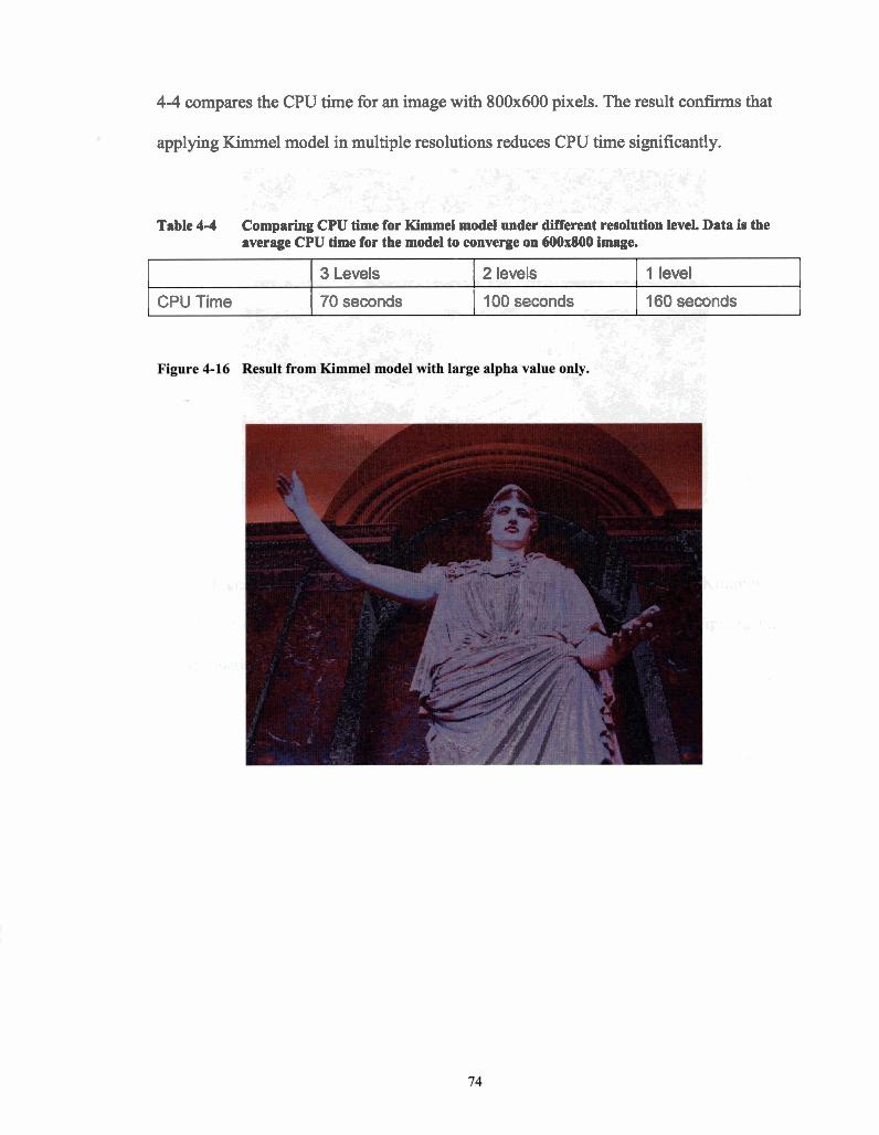
4-4 compares the CPU time for an image with 800x600 pixels. The result confirms that
applying Kimmel model in multiple resolutions reduces CPU time significantly.
Table 4-4 Comparing CPU time for KimmeI model under different resolution level Data is the average CPU time for the model to converge on 600x800 image.
r I 3 L ~ V ~ I S I 2 levels I I level I I CPU Time 1 70 seconds 1 100 seconds 1 160 seconds I

Figure 4-17 Result from Kimmel model with small alpha value only.
Figure 4- 1 8, Figure 4- 19, Figure 4-20 and Figure 4-2 1 show result of Kimmel
model with two levels of a value. The result is compared to combined cusp clipping and
transformation. The original image is provided as well.

Figure 4-18 Kimmel Result I: Kimmel model can recover clouds in the sky.
Original Clipped only
- Kimmel Model

Figure 4-19 Kimmel Result II: Flower
Original
3mmel Model

Figure 4 3 0 Kimmel Result ILL
Original
Kimmel Model
Clipped only

Figure 4-21 Kimmel Result IV: From Louvre Museum
Original
Kimmel Model
4.6 Summary of Gamut Mapping
In this section, we studied gamut mapping between electronic displays.
Previously, the focus of gamut mapping was between monitors and printers, which have a
very different gamut characteristics. We used similar shape gamut property to reduce the
CPU time required for the model and improve quality of existing GMAs.

Two general gamut mapping algorithms, device based and content based, were
discussed in this section. Device based algorithms generally require less time. We
showed that transforming gamuts in XYZ space to fit most of the OOGs inside gamut,
improved the quality of the output image. This linear transformation addresses goals of
non-linear compression and run much faster than non-Linear Models. Applying this
transformation, reduces CPU time required for clipping algorithms as well. This is
because the number of OOGs reduced after the transformation and thus less mapping is
required.
The last part of this section studied two approaches for content-based gamut
mapping. A model to preserve spatial luminance was discussed. This model has the
advantage of requiring less CPU time compared to the other content-based GMAs.
However, the algorithm is useful for computer generated images in which preserving
luminance is quite important. Text is a special case of computer generate images, and
having a rectangular filter compared to square filters for other image type, can improve
the model result.
Kimmel introduced a variation to content-based gamut mapping that is closely
related to a recent variational framework for Retinex. The advantage of his model to
existing models that tried the same idea is speed. He uses an approximation to the
perceptual difference between the original image and mapped one by calculating
smoothed image deviation. In the thesis, it was shown that gamut mapping is a quadratic
programming and if the target gamut is convex, Kimmel approach guarantees
convergence. This is a good approach, since we found that LCD and CRT displays have a
convex gamut. To avoid halo effects in the mapped image, output of two levels of a
values (small and large) were combined. In the locations with higher image variation and
strong edge, large a has a higher weight compared to small a and vice versa. To speed up
the model, the algorithm was repeated in a multi-resolution fashion and updates from the
lower resolution were used as the initial solution for the next higher resolution.
We observed that outputs from this model are better than the other ones
mentioned in this thesis, at the cost of longer CPU time. The other drawback of this
model is having too many variables whose optimal values depend on image type. These
factors are Gaussian mask size, Gaussian variance and z.
Combining a linear transformation with straight clipping has a performance that is
comparable to the Kimrnel model. This is quite important, since our model is a real-time
algorithm and can be used for applications such as remote surgeries, where people need
to preview the result in real time.

CHAPTER 5: DLP PROJECTOR
5.1 DLP Technology, Introduction
Digital Light processingTM (DLP) was designed in 1996 by Texas Instrument.
Today, DLP-based projectors are found in such diverse applications as mobile (ultra-
portable), conference room, video wall, home theatre, and large-venue.
DLP projectors are based on Digital Micromirror ~ e v i c e ~ ~ (DMD) that was
introduced in 1996 by Texas Instruments [35]. The DMD consists of an array of movable
micro-mirrors fbnctionally mounted over a tray, CMOS SRAM [34]. Each mirror is
independently controllable and is used to control reflection of light on a specific pixel.
These mirrors are controlled by loading data into the memory cell located below the
mirror. Many DLP projectors have a colour wheel with 4 different filters (Red, Green,
Blue and White). Recently, there are new modifications to DLP technology that includes
more than 4 colour filter. Some DLP technologies for Digital Cinema only include three
colours (Red, Green and Blue). This is mainly done to avoid flickering effect in fast
moving frames [39]. However, in this thesis we only consider characteristics of DLP
projectors with 4 primary colours. These DLP projectors have a white channel in addition
to RGB channels to enhance mid-to high image frequencies. The algorithm for applying
the white filter was published by Texas Instruments in 1998. The white filter is added in
3 fixed amounts. At each transition point, the RGB values are modified to maintain a

smooth luminance ramp without hue shifts [30]. Some of the interesting characteristics of
DLP projectors are as follows [34] and [38]:
Except for the AID conversion at the front end, all the data processing and
display in DLP displays are digital.
DMD display resolution is fixed by the number of mirrors on the DMD.
This effect combined with the 1 : 1 aspect ratio of pixels necessitates re-
sampling of input video formats to fit on the DMD array with constant
number of mirrors.
To generate different shades of grey, mirrors can tilt 10 degrees towards lights,
ON state, or 10 degrees away from light, OFF state [36]. For instance, when the mirror
switches OFF more than ON, it reflects a darker grey pixel. Colour is added by placing a
light filter (colour wheel) between light source and DMD panel. When it spins, it causes
red, green and blue light to fall sequentially on a DMD micro mirror. For example, a
purple pixel is created by tilting a mirror towards light source when blue and red light
falls on it and letting green light to go through (not reflected). Because DMD mirrors can
work binary by allowing light to get reflected or pass through, they have a better dark
value and less light leaking when R=G=B=O.
Another advantage of DLP projectors over LCD displays is their small or non-
existent image lag. Image lag has been a major limitation of LCD-based video projectors.
Because of the response time of the liquid crystal molecules to the applied fields and the
relaxation times when the fields are removed, some of the image from one frame carries
over into the next, which gives rise to image lag [34].

5.2 DLP Projector Characteristic
In this section, we briefly check over some of the DLP projector characteristics.
The two DLP projectors used in this thesis are as follows:
Table 5-1 DLP projectors used in this thesis
These DLP projectors, similar to the CRT displays, exhibited significant channel
dlp-Toshiba
dlp-lnfocus
interaction (Figure 5-1). This interaction is calculated using equation (2) introduced in
Toshiba TDP-5 DLP Projector
lnfocus DLP LP1 Projector
Section 2.3. The interesting observation is that when each primary is ramped from 0-255
while the other two channels are set to 255, the primary has a higher intensity than when
either of the other two channels is set to zero. This is because of the additive effect of the
white filter. The other interesting observation is that in both devices in all their 3
channels, the white filter is added around 1 15 digital count of a primary when the other
two primaries are set to 255. (e.g. R=115, G=B=255).

Figure 5-1 Channel Interaction for DLP projector. The horizontal axis represents the input value v ranging from 0 to 255 and the vertical axis represents the value of the channel interaction metric, ClcoLoR(v,a,b). The black line shows a=b=255 and dark and light dashed lines show a=O,b=255 and a=255,b=0 respectively. For instance, on Green Interaction, light grey represents CI when R=255,B=0 and G ramps from 0-255.
Another potential issue that was considered for LCD and CRT displays is having
a possible chromaticity shift. Figure 5-2 shows the chromaticity coordinates for each of
the primary colours (RGB), as well as the combined colours (CMYK), after dark
correction, plotted at 10 luminance settings per colour. Both DLP projectors have stable
RGB chromaticity. Interestingly, Magenta and Yellow have stable chromaticity while
Cyan shifts towards green as it ramps to 255. This behaviour can be explained by looking
at Figure 5- 1, which shows that Green and Blue have different channel interaction (CI)
depending on which channel is set to 255 (i.e. a=255,b=0 or a=O,b=255). Cyan shifts
towards Green, since Green has high CI when R=O,B=255 while Blue has low CI in this
setting.

Figure 5-2 Chromaticity shift for DLP projectors shown as intensity is increased plotted in xy space with x=X/(X+Y+Z) on the horizontal axis and y=Y/(X+Y+Z) on the vertical axis. When there is no chromaticity shift, all the dots of one colour lie on top of one another and therefore appear as a single dot. R,G,B,C,M,Y,W represent ramps of Red, Green, Blue, Cyan, ~ a i k n t a , Yellow and White (r=g=b)
dlp-toshiba
Channel Interaction (CI) in white is explained by additive effect of the white
filter. The Next section discusses effect of the white filter on the existing calibration
models.
5.3 Calibrating DLP Projectors
An end-user, as opposed to the manufacture, may well wish to characterize and
calibrate a DLP projector in order to control accurately the colours displayed. The end-
user's task is complicated by the fact that the precise internal workings of the projector
are unknown. In this section we study methods for end-user colour calibration of 4-wheel
DLP projectors.
As was mentioned earlier, the white filter in 4 channel DLP projectors is added in
3 fixed amounts to enhance mid and higher frequencies. Because the white filter simply
adds another additive component to the already existing RGB channels, it is possible that

a 3x4 matrix can characterize tristimulus values. The amount of white added depends on
the summed luminance of RGB channels and the target expected luminance. The logic
for the model is published, but since there are parameters that are calibrated for each
projector separately, the end-user cannot use the logics published by Texas Instruments to
predict the output of DLP projectors accurately.
Stone in [lo] mentions the idea of using 4 channels for calibrating DLP displays,
but the calculations for the white LUT is not specified. In this section, we first look at
basic Linear Model and its results when applied to DLP projectors. Then results of a
model introduced by Wyble [64] and a modification to his model are discussed and they
are compared to the performance of the Masking Model [2].
5.3.1 Linear Model for DLP Projector
The Linear Model was implemented as explained in section 2.4.2. This model was
not expected to perform accurately because of the white filter. Interestingly, this
model performed quite accurate, in predicting tristimulus values for low-to mid
brightness colours(Figure 5-3).

Figure 5-3 Linear Model Result on dlp-Toshiba projector. R and G are chromaticity channels represents r/(r+g+g) and g/(r+g+b respectively. The vertical axeu represents error in &.
DLP calibration compare
53.2 Number of Channels Required
As was mentioned earlier, it was suggested that extending the Linear Model to
have 4 channels rather than one should perform accurately for DLP projectors. However,
the challenging part is to design the 4 channels so that the model can predict the white
factor accurately.
Principal Component Analysis (PCA) is used to find the number of base required
to represent the space accurately. We define the space as the combination of linearized
channels and tristimulus values. For instance the scores of the base for PCA applied to a
model that gives R',G',B', W out of RGB, represents the importance of each basis to
represent the space [R' ,G',B ' ,W,X,Y ,Z].
One way to derive 4 channels is to define W=min(R,G,B), B'=B-W, G'=G-W and
B'=B-W. Note that W in this case is similar to K in masking model. For consistency with
the Wyble model we use W instead of K in this chapter. Table 5-2 shows the scores for
this space. Looking at this space (R'G'B'W), it is obvious that 4 basis is not enough to
explain all the data in the space created by R'G'B'WXYZ. A similar effect is seen for
RGB (Linear Model).
The other method to represent 4 bases is to use RGB as the new basis and add
W=min(R,G,B). The third row of Table 5-2 shows that in this new space, 4 bases should
be sufficient to define the whole space and thus provide a model to accurately predict
XYZ from RGBW. This model was first introduced by Wyble [64] and will be discussed
further in the next section.
The last space considered is created using the Masking Model. Implementation of
this model was discussed earlier in Section 2.4.3. This model can be inverted to predict
RGB given XYZ values. As shown in the last row of Table 5-2, the 7 bases should be
sufficient for deriving an accurate calibration model for DLP projectors.
Table 5-2 Scores for bases of PCA applied to each space. Scores are Residual Variance of each principal component. The scores can be used as an indication for the number bases required to sufficiently describe a space.
Number of Basis Vectors
RGB
R'G'B'W
RGBW
R'G'B'C' M'Y'W
B1
51
60
1.5
1.5
82
9.1
9.6
.3
.3
B3
4.9
7.1
.3
.3
B4
2.7
3.5
.2
. I 7
B6
.04
1.7
.OO
.OO
B5
.ll
2.5
.OO
.OO
B7
- .7
.OO
.OO
B8
- - -
.OO
5.3.3 Wyble's Model for DLP Projector Calibration
Wyble [64] uses RGBW basis vectors to calibrate DLP projectors. He also
introduces a method for predicting RGB values given XYZ data. R,G,B and W are
derived using rLUT, gLUT, bLUT and wLUT. R, G, and B LUTs are normalized values
of the X, Y, and Z values respectively, of the red, green and blue ramps. The white LUT
must account for that part of the colour that exceeds what the combined RGB channels
would produce. Y values of ramps of grey minus the Y values of the red, green, and blue
ramps for are used to create wLUT. Figure 5-4 shows that wLUT with respect to X,Y,
and Z are very similar to each other.
Figure 5-5 shows the jLUTi, where j€(R,G,B}, i€{X,Y,Z}. This figure shows that
having a combination of the three LUTi for each channel is not important since all the
LUTs for each channel are quite similar. rLUTz seems to behave differently and it is
because values of this LUT is quite small and normalizing the LUT puts emphasize on
variations due to possible noise in measurement.

Figure 5-4 White LUT for dlp-Toshiba. All three LUTs have similar shape

Figure 5-5 The LUTs for the four channel of Wyble's model. *
-0.5 1 I I I I I
0 50 100 150 200 250 300 Ramps of Red
Ramps of Green Three bLUT
"0 50 100 150 200 250 300 Ramps of Blue
Three WLUT
0 50 100 150 200 250 300 Ramps of White

After the RGB values are linearized and the R'G'B'W are derived, a 3x4 matrix M3x4 is
used to transform linearized values to XYZ space. Wyble defines M3x4 as follows:
In (20) X,Y, and Z are measured tristimulus values and the subscript R,G,B,W are for
maximum digital values for red, green, blue and white. The super-script C shows that all
the values are used after black-correction ( XYZ values for R=G=B=O is removed).
The backward model is quite complicated. Theoretical RGB values, RGBtho,, is
calculated by applying the inverse matrix of the left most three columns of M3x4 to the
input XYZ. Let us call this matrix M2. The calculated RGB values are theoretical since
they can have values greater than 255. This is because the effect of the white filter is not
taken to account yet. To remove the white filter effect, three look up tables, wLUTj, are
created for each red, green and blue channels separately. The following steps are used to
create wLUT,:
Forr=Oto255
Calculate XYZ values of digital count (r,255,255) using forward model
Calculate RGBth, by apply M2 to the corresponding XYZ values
The wLUTr uses Rth, as the index and r as the output
The white-filter effect is calculated as follows:
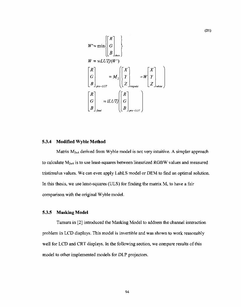
5.3.4 Modified Wyble Method
Matrix M3x4 derived from Wyble model is not very intuitive. A simpler approach
to calculate M3x4 is to use least-squares between linearized RGBW values and measured
tristimulus values. We can even apply LabLS model or DEM to find an optimal solution.
In this thesis, we use least-squares (ULS) for finding the matrix M, to have a fair
comparison with the original Wyble model.
5.3.5 Masking Model
Tarnura in [2] introduced the Masking Model to address the channel interaction
problem in LCD displays. This model is invertible and was shown to work reasonably
well for LCD and CRT displays. In the following section, we compare results of this
model to other implemented models for DLP projectors.

5.3.6 DLP Calibration Results
In this section, we compare the forward and backward error in AEg4 similar to
what was done in Chapter 2. The results are based on 2277 measurements. Each points
was measured 5 times and repeated 3 times throughout the whole measurement.
Table 5-3 shows the forward error for 5 models discussed earlier. R'G'B'W was
shown earlier that is not expected to perform accurately since the PCA of its space
required more than 4 channels. Modified Wyble is the small change to derive
transformation matrix. This table shows that Modified Wyble and Masking Model
perform very accurate and since Modified Wyble uses a smaller matrix transformation, it
may be desirable.
Table 5-3 Forward Calibration Error in AE94 for DLP projectors based on 2277 points.
Dlp-Toshiba
Dlp-lnfocus
It is also interesting to consider points that each model failed on predicting them.
Figure 5-6 shows that Wyble model performed poorly, mainly for bright colours. The
model was not successful in removing the white filter completely.
Std
Mean
Max
Std
Mean
Max
4.69
Linear
7.4983
16.67
3.24
9.08
19.7
4.54
Wyble
3.27
11.57
3.42
4.18
12.00
.453
Modified Wyble
1.04
3.44
.63
.814
3.34
4.0354
R'G'B'W
3.16
1 1.82
1.97
5.42
21.75
.998
Masking
1.01
3.53
.774 -
.871
3.376

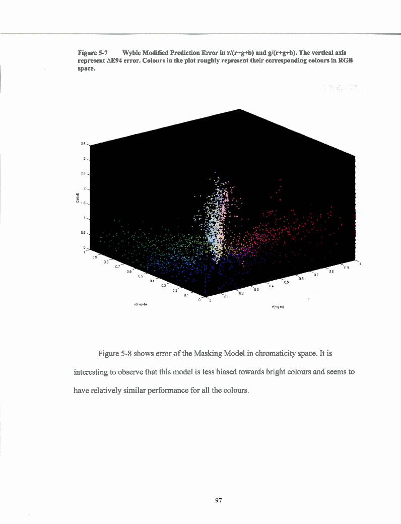
Figure 5-7 Wyble Modified Rediction Error in r/(r+g+b) and g/(rkg+b). The vertical asis represent AE94 error. Colours in the plot roughly represent their corresponding colours h RGB space.
Figure 5-8 shows error of the Masking Model in chromaticity space. It is
interesting to observe that this model is less biased towards bright colours and seems to
have relatively similar performance for all the colours.

Figure 5-8 Masking Model Error in r/(r+g+b) and gl(r+g+b). The vertical axis represent AE94 error. Colours in the plot roughly represent their corresponding colours in RGB space.
DeileE prediction using RGBCMYK method
Comparing the backward error is more interesting. As shown in Table 5-4 The
Masking Model outperforms Wyble in the backward direction. Backward error is
calculated by predicting RGB values for a given XYZ input and the applying the forward
model to predict the XYZ of the RGBbackward. The difference between the input and
predicted XYZ is used to calculate AEg4 and the error is adjusted by subtracting data fiom
forward model. Modified Wyble Modified is used to calculate XYZ output of RGBbhd
for Wyble Model.

Figure 5-9 and Figure 5-1 0 represent error distribution of the two model for
forward and backward prediction.
Table 5-4 Backward Error in AEY4
Dlp-Toshiba
Dlp-lnfocus
Mean
Max
Std
Mean
Max
Std
Wyble
2.12
9.53
6.05
4.14
26.12
5.73
Masking
.354
4.45
.584
.3264
2.75
.346

Figure 5-9 Distribution of Forward and backward error for Wyble Model. Left and right columns represent the forward and backward error distributions respectively. Top and bottom rows represent the dlp-Toshiba and dlp-Infocus displays.

Figure 5-10 Distribution of Forward and backward error for the Masking Model Left and right columns represent the forward and backward error distributions respectively. Top and bottom rows represent the dlp-Toshiba and dlp-Infocus displays.
From the above results, we can conclude that both the Modified Wyble and
Masking Models are accurate in predicting XYZ, while the Masking Model is the best
choice for going backward.
5.3.7 Summary of DLP Calibration
We compared possible spaces in which DLP calibration could be applied and we
found that the RGBW and RGBCMYK spaces derived from RGB space can predict
tristimulus values well. Wyble introduced a model that uses a 3x4 matrix to predict XYZ

values. A simple modification to his model can improve forward prediction accurracy.
The Masking Model has similar error performance to the modified Wyble model in
forward prediction (RGB to XYZ). However, we found that the Masking Model is not
biased towards non-bright colours; whereas, the Wyble Model has really good
performance for dark colours but its performance gets worse as the colours have a higher
RGB value. Going backward, the Masking Model performs better than Wyble model in
predicting RGB values.
5.4 DLP Projector Gamut
In this section, we study the gamut of DLP projectors and consider which GMAs
discussed earlier are the best choices for DLP displays. Figure 5-1 1 and Figure 5-12
represent the gamut shape of the two projector in XYZ space. These two figures show
that DLP projectors clearly have a concave gamut. The white-filter effect can be assumed
as the main reason for causing the concavity in DLP gamut. Interestingly, the projectors
have a very similar looking gamut.

Figure 5-11 Gamut shape of dlp-Infocus Infocus DLP Gamut in xyz space . I .
1
Figure 5-12 Gamut of dlp-Toshiba
-
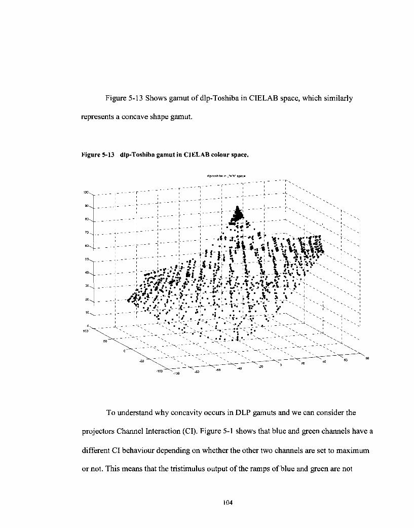
Figure 5-13 Shows gamut of dlp-Toshiba in CIELAB space, which similarly
represents a concave shape gamut.
Figure 5-13 dlp-Toshiba gamut in CIELAB colour space.
dlp-tosh~bs ~n L.seb'opece
To understand why concavity occurs in DLP gamuts and we can consider the
projectors Channel Interaction (CI). Figure 5-1 shows that blue and green channels have a
different CI behaviour depending on whether the other two channels are set to maximum
or not. This means that the tristimulus output of the ramps of blue and green are not

completely additive effect of the 3 primaries (red, green and blue lights), and there are
some additional factors (in this case the white filter) that makes them behave differently.
Since the red channel has a consistent CI, mostly increasing, independent of the other two
channel settings, we can expect that the gamut boundary created by the ramps of red
channel to have a convex shape. On the other hand, we should expect concavity on parts
of the gamut with ramps of blue and green, since some artificial factor made their channel
interaction to behave differently. This effect is shown in Figure 5-14, where the red and
blue dots represent ramps of Red and Blue, respectively, while the other two channels are -
set to maximum.
Figure 5-14 Ramps of Red and Blue on the gamut when the other two channels are set to maximum.
This figure shows that on the part with ramps of red, the gamut is quite convex
compared to the part with blue ramps.
This is an interesting observation since it allows us to predict possible locations in
the gamut that are likely to be concave. Extending this idea to the printer technology can
be quite useful especially since studying printer gamuts with 7 or more inks is quite
challenging.
For printers, concavity can occur because of the ink-interaction and the ink-
separation. Ink separation tells what ink combination to put down for a given RGB value.
By studying the CI of RGB input values, we may be able to predict concavities that occur
because of the ink-separation. Being able to remove these concavities can allow for
expansion of the gamut and predicting the gamut boundary more accurately.

CHAPTER 6: LCD PROJECTOR VERSUS DLP PROJECTOR
In this section, we compare some of the characteristics of LCD and DLP
projectors. In particular, two of the main projectors characteristics are Temporal Stability
and Spatial Non-Uniformity. In this study, two LCD and two DLP projectors were used.
Table 6-1 shows the projector names used in this study.
Table 6-1 Projector names used I 1 I
Name
PR1
PR2
6.1 Temporal Stability
Temporal Stability indicates the amount of time it takes for the projector bulb to
stabilize after it is turned on [42]. Full Red, Green and Blue were measured every 5
seconds for 45 minutes starting from the time that the projector was turned on. To
improve the quality of the data, we made sure that before each test, projectors had been
turned off for at least 5 hours for the bulbs to cool down. Figure 6-1 shows that Green
and Blue channels have a big shift in their chromaticity as the LCD bulb warms up. On
Description
Proxima LCD Desktop Projector 9250
Proxima LCD Ultralight LX
dlp-Toshiba
dlp-Infocus
Toshiba TDP-5 DLP Projector
Infocus DLP LP 1 Projector

the other hand, DLP projectors seem to have stable chromaticity fiom the very beginning,
when they are first turned on.
Figure 6-1 Temporal Stability for 2 LCD and 2 DLP projectors. In the first 3 columns, changes in R, G and B channels are shown. Horizontal Access represents d(x+y+z) and y/(x+y+z). Vertical access represents the data measurements.
pR2 PR? PR2 Intensity
dipinfocus Intensity
apt- '+t@=f- - dlptmhiba Intensity

6.2 Spatial Non-Uniformity [42]
The spatial non-uniformity was considered by displaying a full white image and
measuring the tristimulus values at 9 corner positions on the screen. Figure 6-2 shows
the 9 comers of the screen that were measured.
Figure 6-2 6-3 The 9 points of screen measured to verify Spatial Non-Uniformity. 'C', 'R', 'L', 'T' and 'B' stand for Centre, Right, Left, Top and bottom corners. RB, LB are Right-Bottom and Left-Bottom locations.

Figure 6-4 Spatial Non-Uniformity. The first column shows white measurements at 9 different locations on the screen for each display. Second column represents intensity (X+Y+Z) of white at each location. 'C', 'R', 'L', 'T' and 'B' stand for Centre, Right, Left, Top and bottom corners. RB, LB, RT and LT are Right-Bottom, Left-Bottom, Right-Top and Left-Top locations.
PRt
dlp-infocus
N
t oo
dlptoshiba
PR1 lntensity 350 1
PR2 lntensity
RBk
dlpinfocus lntensity
3 0 0 ~ Bk
dlptoshiba lntensity
LBl

Table 6-2 shows the error in AEg4 caused by Spatial Non-Uniformity in projectors. It
shows that DLP and LCD projectors have a very similar Spatial Non-uniformity.
Table 6-2 Error caused by spatial non-uniformity for projectors.
Mean AEg4
DLP Projector
LCD Projector
Max AEg4 Std AEg4
10.09
7.99
20.67
19.15
7.62
6.31

CHAPTER 7:DEVICE CALIBRATION VIA SUPPORT VECTOR REGRESSION
7.1 Introduction
The problem with the previous models for calibrating the CRT, LCD or DLP
displays is that the user needs to know some details about the internal structure of the
device. For instance, the user needs to know about the effect of the white filter in DLP
technology to approach the models such as Masking or Wyble models.
In this section, we present a new approach based on training to calibrate displays.
In this approach, users do not need to have any internal information about the internal
technology of displays.
Vapnk's Theory of Support Vector Machine ([60][61]) has been applied to a wide
variety of problems [63] including the recent application on Estimating Illumination
Chromaticity by Funt and Xiong [59].
There are several advantages for using SVR over existing statisticalltraining
models. SVR is known to perform better than other models (e.g. Neural Network) on
sparse data set and it can achieve global optimum rather than locally optimum solution.
Given a set of input and corresponding output values, SVR tries to assign a
relationship (function) between the data by applying regression. This function can be
used for prediction, including data that was not included in training set. This model is
quite similar to Neural Network with the difference that Neural Network stops at a local
optimum solution; whereas, SVR achieves a global optimum. SVR, similar to the Neural

Network feedback loop, requires a loss function to calculate estimation error. If the
original problem is non-linear, the kernel trick can be applied to reformulated the
problem in terms of a kernel function.
SVR tries to ignore the points that are out of its prediction range. It uses E values as
to represent the range of its prediction. Figure 7-1 illustrates the &-insensitive for points
that fall out of the maximum error range.
Figure 7-1 SVR Error Insensitive Case. Data points outside the error range are ignored
E (maximum error allowed)
\
Error off the road is counted. Since it is larger than E, then it is ignored
A geometric representation of SVR is given by Bi and Bennet [65]. If training data
set are linearly separable, SVR classifies the data by finding the separation plane with the
maximum hard margin between classes. Figure 7-2 shows a geometric representation of

the SVR. It shows that when SVR is applied to a set of points, it finds the closest point in
convex hull of the data from each class.
Figure 7-2 SVR Classification. SVR computes the closest point in convex hull of the data from each class
I)'
7.2 Applying SVR to Calibration Problem
RGB values were used as input values and L*, a*, b* separately as output data.
Euclidean distance between estimated points and original input values is used as an error
measurement function.
SVR performance is known to depend on the insensitivity parameter, E, and the
choice of kernel function used to associate data points. The four most common kernel
functions are shown in Table 7-1.

Table 7-1 Four most common choices for Kernel function. d is the parameter to be set
I Name I Equation I I Linear I K(xixj) = (xi)Txj I I Polynomial I K(xixj) = [(xi)Txj+l]d I I Radial Basis Function (RBF) I K(xixj) . ed 11 xi-xiI12 I
For calibrating our display we experimented with Polynomial and RBF type
functions. Sigrnoid was not used because it could not classify the data accurately and it is
not defined for some specific d values. The kernel choice and parameter setting (cost
value and d) were set by choosing 200 data points out of 1000 possible values randomly
for 20 times. C value ranged from [.I-81 and d values ranged from [.01-.5] and [I-81 for
RBF and Polynomial kernel respectively. Nedler-Mead Simplex search with multiple
random initialization point was used to find an optimum setting.
Sigmoid
7.3 Results
Below are the results for apply SVR model to predict tristimulus values. 300
colours were chosen randomly out of 2277 measured data point for training purpose. The
model was evaluated on the 2277 colours including training data. However, it was found
that the SVR performs similarly for CRT and LCD display characterization, if only
tristimulus values of ramps of red, green and blue are used. Interestingly, for some
displays, the performance is better than DEM model.
K(xixj) = tanh[(xi)Txj+d]
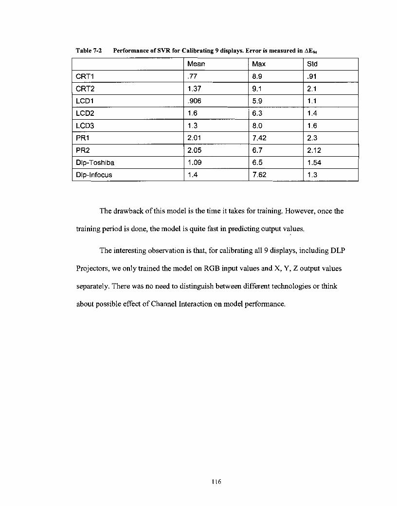
Table 7-2 Performance of SVR for Calibrating 9 displays. Error is measured in AE94
I I Mean I Max 1 Std I
I I I
Dlp-Toshiba 1 1.09 1 6.5 1 1.54
CRT2
LCD I
The drawback of this model is the time it takes for training. However, once the
training period is done, the model is quite fast in predicting output values.
The interesting observation is that, for calibrating all 9 displays, including DLP
Projectors, we only trained the model on RGB input values and X, Y, Z output values
separately. There was no need to distinguish between different technologies or think
about possible effect of Channel Interaction on model performance.
1.37
.906
9.1
5.9
2.1
1 . I

CHAPTER 8:CONCLUSION
An end-user may well wish to analyze and predict behaviour of electronic
displays without knowing about having knowledge to internal structure of the devices.
The focus of this thesis is to address this need and study possible improvements we can
give to already existing models.
Characteristics of CRT and LCD monitors and projectors were studied. It was
shown that LCD displays do not have significant Channel Interaction once the displays
are made for end-user. Some characteristics such as longer than normal time to stabilize
colour output on CRT monitors were pointed out. A good measurement model for the
displays was discussed. Implementation of 3 calibration models, 3D LUT, Masking
Model and Linear Model were studied. Linear Model has better performance on both
CRT and LCD technologies since the channel interaction and chromaticity shift is
removed for end-users. A simple extension to Linear Model (Linear+) can improve white
balancing.
Two new algorithms were introduced that try to optimize existing calibration
models by considering the importance of the colours in a space that matters to us. These
two models (LabLS and DEM) were shown to improve calibration for CRT and LCD
displays by around 10%.
Gamut mapping is another important factor since more and more people are
viewing documents and images on electronic displays. In applications such as remote
surgery, users need to be able to view important features of an image even if they are
viewing the objects on different types of display Some of these applications require a real
time mapping. In this thesis, we specifically considered gamut mapping between
electronic displays (CRT and LCD displays). Implementation of device-based and
content-based gamut mapping were discussed. The performance of 4 different device-
based Gamut Mapping algorithms was compared and it was shown that numerically
these algorithms tend to have similar performance. However, visual comparison showed
that Straight Clipping performs better than other device-based GMAs, by preserving
contrast rather than colourfulness in an image. Implementation and performance of a
model intended preserve Spatial Luminance in an image was discussed and we observed
that this model does not improve quality of device-based GMAs on scene images. This
model can be a good choice for computer generated images and a simple modification to
the model was shown to improve the output of images with text.
Kimmel introduced a mathematical approach to gamut mapping algorithms that
guarantees finding an optimum solution if the target gamut is convex. We observed that
this model can recover most of the lost spatial information in an image because of
applying other GMAs at the cost of much longer CPU time.
We introduce a model that takes advantage of similar gamut shapes of CRT and
LCD displays to have output quality similar to content-based GMAs and at the same
time require CPU time as low as device-based GMAs. This model uses a transformation
based on reference colours in LCH space and applied Straight Clipping to remaining Out-
of-gamut colours. It also can take less CPU time compared to fast device-based GMAs by
trying to fit most of source gamut inside the target gamut in a linear transformation.

New projector technology (DLP) has the fourth channel (white) added to the
existing ones that increases image luminance. We showed that the best space to have
calibration is derived spaces with 4 or 7 bases from RGB channels. A basic modification
to the Wyble Model was shown to improve the forward prediction significantly.
Applying the Masking Model with 7 bases has similar accuracy in predicting XYZ values
given digital input data. However, in the backward direction (XYZ to RGB) we observed
that applying Masking Model has a much better accuracy than the Wyble model. Thus,
using this 7 bases model improves overall calibration result for DLP projectors.
Other characteristics of DLP projectors such as Channel Interaction and
Chromaticity shift were studied. We showed that using behaviour of Channel Interaction
on each channel we can predict places that gamut can have concavity. It is an interesting
observation and applying it to printer models can improve gamut of printers, especially
ink-jet printers with large number of inks (7 or more).
In the last part of the thesis, a new model using Support Vector Regression was
introduced for colour calibration of electronic displays including DLP projectors.
Interestingly, by using SVR user does not need to know weather 3 or more bases are
needed to predict XYZ values accurately. SVR can prediction 3 functions that predict X,
Y and Z output values given RGB input data. The other observation was that this model
can in some cases outperform that LabLS and DEM model.

CHAPTER 9: CONTRIBUTION SUMMARY
The first part of this thesis on display characterization represents a joint effort
involving both myself and Bill Cressman. This work is published in a conference paper at
CGIV2004 and a journal paper CR&A. The characterization models were implemented
in Matlab, and were largely a joint effort. Module ownership was roughly divided such
that Mr. Cressman primarily developed the 3D LUT and backward Masking Model
engines, while I developed the Linear Model and the forward part of Masking Model
engines. With respect to data analysis and model testing, Mr. Cressman focused on
analysing measurement error and the effects of channel interaction. I focused on possible
reasons behind channel interaction and studying the effects of chromaticity shift.
Optimal Colour Calibration was a joint work between my supervisor, Dr. Funt,
Mr. Roozbeh Ghaffari and myself. Dr. Funt and I focused on LabLS model and Mr.
Ghaffari studied the DEM model.
In the gamut mapping section, I studied the most popular mapping algorithms in
this field. I specifically did not try to introduce any new GMA for mainly two reasons.
First, measuring the performance of a GMA is greatly influenced by: the test-image
content, which type of GMA application is used and the viewing condition. Thus it is
generally quite hard to decide whether one mapping is better than other available
mappings. The other reason is based on TC8 Committee decision to standardize GMAs
so that there are a few world-wide known algorithms [14].
DLP Calibration is completely my own work, which started by studying
characteristics of DLP projectors and introducing a model that improves existing
algorithms.
In the DLP calibration section I extended the idea from paper by Dr. Funt and Mr.
Xiong [59]. Mr. Xiong helped me with the initial understanding of the model.

REFERENCE LIST
R. Balasubramanian, "Reducing the Cost of Lookup Table Based Colour Transformations", Colour Imaging Conference vol44, no.4; 1999 p. 32 1-327
N. Tamura, N. Tsurnura, Y. Miyake, "Masking Model for accurate colourimetric characterization of LCD" Proc. IS&T/SID 10th Colour Imaging Conference 2002 p. 3 12-3 16.
S. R. Bums, "Methods for Characterizing CRT displays", Displays, vol 16, Issue 4, 1996, p. 173-1 82
IEC 61966-4: Multimedia system and equipment: Colour measurement and management. Part 4: Equipment Using
E. D. Montag and M. D. Fairchild , "Gamut mapping: Evaluation of chroma clipping techniques for three destination gamuts." IS&T/SID Sixth Colour Imaging Conference, Scottsdale, 1 998, p. 57-6 1.
G.J. Braun and M.D. Fairchild, "Gamut Mapping for Pictorial Images." TAGA Proceedings, 1999, p. 645-660.
R. Balasubramanian, R. deQerioz, R. Eschbach and W. Wu, "Gamut Mapping to preserve spatial luminance variation'. Journal of Imaging Science and Technology, vol. 45, no. 5 2001
R. Kirnmel, D. Shaked, M. Elad, I. Sobel, "Space Sensitive Colour Gamut Mapping: A Variational Approach." HPL-2000-50,2002
G. Hurnphreys, I. Buck, M. Eldridge, P. Hanrahan, "Distributed Rendering for Scalable Displays," IEEE, Supercomputing, 2000
M. Stone, "Color Balancing Experimental Projection Displays", IS&T Ninth Color Imaging Conference, 2001,342-347.
Schmidt. Schmidt's Glossary of Terms, cited November 2004, http://www.schmidt.com/WorkWith/displayItems/displayGlossary.cfm?l=c
J. Morovic, "To Develop a Universal Gamut Mapping Algorithm, Phd Thesis, University of Derby, 1998
J. Morovic, M. Lou, "The fundamental of Gamut Mapping: A Survey", Journal oflmaging Science and Technology, vol. 45, no. 3,2001
Morovic, J., CIE Division 8, cited November 2004, http://www.colour.or~tc8- 031 -
McDonald, L.W., Gamut Mapping in Perceptual Color Space, Proceeding lSt IS&T/SID Color Imaging Conference. Springfield, VA, 1993, 193- 196

P. Hung and R.S. Berm, "Determination of Constant Hue Loci for a CRT Gamut and Their Predictions Using Color Appearance Spaces", Color Research and Application, vol. 20, no. 5, 1995, p. 285-295
F. Ebner, M.D. Fairchild, "Finding Constant Hue Surfaces in Color Space", Proceedings of SPIE, Color Imaging: Device-Independent Color, vol. 3300- 16, pp. 107-1 17, 1998
J.J. McCann "Color Gamut Measurments and Mapping: The Role of Color Spaces", Proceedings of SPIE Electronic Imaging Conferene, vol. 3648, pp. 68-82, 1999
G.J. Braun, and M.D. Fairchild, "Gamut Mapping for Pictorial Images, TAGA Proceedings", pp. 645-660 1999
CIE 13 1-1 998, "The CIE 1997 Interim Colour Appearance Model" CIECAM97s" (1 998)
Mathworks, Matlab Help, Cited: November 2004, http://www.mathworks.com
C. B. Barber, D.P. Dobkin, and H. T. Huhdanpaa, "The Quickhull Algorithm for Convex Hulls", ACM Transactions on Mathematical Software, vol. 22, no. 4, pp. 469-483, 1996.
Geometry Algorithms, Convex-hull of a 2D Point Set or Polygon, cited November 2004, http://geometryalgorithms.com~Archive/algorithm 01 09/algorithm 01 09.htm
R. S. Gentile, E. Walowitt and J. P. Allebach, "A comparison of techniques for color gamut mismatch compensation", Journal of Imaging Technology., vol. 16, pp. 176-181, 1990.
N. Katoh and M. Ito, "Applying Non-linear Compression to the Three- dimensional Gamut Mapping" ,The Journal of Imaging Science and Technology JulyIAugust, vol. 44, no. 4; pp. 328-333, 1999
E. D. Montag and M. D. Fairchild, "Psychophysical evaluation of gamut mapping techniques using simple rendered images and artificial gamut boundaries, " in Proc. IEEE Trans. Image, pp. 977-989, 1997
S. Nakauchi, S. Hatanaka, and S. Usui, "Color gamut mapping by optimizing perceptual image quality, " in Proc. IS&T/SID Color Imaging Conference., pp. 6347,1996
C.J Li, M.R. Luo, R. W .G. Hunt, N. Moroney, M.D. Fairchild, and T. Newman, 'The performance of CIECAM02", IS&T/SID CIC 10, Scottsdale, pp. 28-32 2002.
M. Fairchild, "Color Appearance Models: CIECAM02 and beyond", tutorial notes, IS&T/SID 12th Color Imaging Conference, 2004
M.C. Stone, "Color and Appearance Issues for Tiled Display", IEEE Computer Graphics and Applications, vol. 21, issue 5, pp. 58-66,2001

CIE, CIE Division 8, cited November 2004, http://www.colour.orp/tc8- 03ltest imag;es.html,
M. Melgosa, R. Huertas, A. Yebra and M. M. Perez, "Are chroma tolerances dependent on hue-angle?", Color Research and Application, vol. 29, issue 6, pp. 420-427,2004
Berns, RIT Research Lab, Cited November 2004, http://www.cis.rit.edulmcsl/research/hueLUTs.shtml
Vishal Markandey, Todd Clatanoff, Greg Pettitt, Video Processor D L P ~ ~ Display Systems Online Technical Report, available at: whitepapers.zdnet.co.uk
L. J. Hornbeck, "A Digital Light Processing update status and future applications", Proceedings of SPIE, vol. 3634, pp. 158- 170, 1999
Sharp, Sharp Display, Cited November, http://www.sle.shar~.co.uk~research/3d/Proiection.htm
DLP, dlp new design, cited November, http://www.dlp.com/about dlp/about dlp FAOs technolony.asp?bhcp=l
G. Marcu, "Color in Electronic Display", IS&T/SID Tutorial Note, Scottsdale, 2004
C. Poynton, B. Walker, J. Pines, J. Goldstone, "Color Appearance Issues in Digital Cinema Exhibition", IS&T/SID Tutorial Note, Scottsdale, 2004
G. Humphreys, I. Buck, M. Eldridge, P. Hanrahan, "Distributed Rendering for Scalable Displays", IEEE Supercomputing no. 30,2000
M. Stone, "Color Balancing Experimental Projection Displays", IS&T Ninth Color Imaging Conference pp. 342-347,200 1
L. Seime, J.Y. Hardeberg: "Characterisation of LCD and DLP Projection Displays". Color Imaging Conference. pp.277-282,2002
OLED Tutorial, Wave, Cited November 2004, http://www.wave- report.com/tutorials/oled.htm
OLED Specification, peripheral, Cited November 2004, peripherals.about.com/cs/monitors/alaa102003a.htm
J. J. McCann, "Lessons Learned from Mondrian Applied to Real Images and Color Gamuts", Proceedings of the IS&T/SID Seventh Color Imaging Conference, pp 1 -8, 1999.
Divergence, mathworks, Cited November 2004, http://mathworld.wolfram.com/Diveraence.html
Quadratic Programming, Mathworks, cited November 2004, http://www.mathworks.com/products/optimization/description5.html

W.W. Hager, Y. Krylyuk, "Graph Partitioning and Continuous Quadratic Programming", SIAM Journal on Discrete Mathematics, , vol. 12, issue 4, pp 500-523, 1999
Amidror I., "Scattered data interpolation methods for electronic imaging systems: a survey", J Electronic Imaging vol. 1 1.2, pp. 157- 176,2002
M.D. Fairchild, D.R. Wyble, "Colorimetric Characterization of the Apple Studio Display (Flat Panel LCD)." Munsell Color Science Laboratory Technical Report, 1 998, http://www.cis.rit.edu/mcsl/research~PDFs/LCD.pdf
Finlayson G.D., Drew M.S., White-Point Preserving Color Correction, Proc. IS&T/SID 5th Color Imaging Conference: Color, Science, Systems and Applications, pp.258-261, Nov. 1997
J.E. Gibson, M.D. Fairchild, Colorimetric Characterization of Three Computer Displays (LCD and CRT), Munsell Color Science Laboratory Technical Report, 2000, , htt~://www.cis.rit.edu/mcsl/research~PDFslGibsonFairchild.~df Y. Kwak, LW. MacDonald, "Accurate Prediction of Colors on Liquid Crystal Displays", Proc. IS&T/SID 9th Color Imaging Conference 355-359,2001
Y. Yoshida and Y. Yamamoto , "Color Calibration of LCDs". Proc. IS&T/SID 10th Color Imaging Conference pp. 305-3 1 1, 2002
G. Marcu, "Tracking Correction for TFT-LCDs", Proc. IS&T/SID Tenth color imaging conference, pp. 272-276,2002
Lagarias, J.C., Reeds, J. A., Wright, M. H. and Wright, P. E., "Convergence Properties of the Nelder-Mead Simplex Method in Low Dimensions," SIAM Journal of Optimization, vol. 9 Number 1, pp. 1 12-1 47, 1998.
Balasubramanian, R., Color Transformations for Printer Color Correction, Second Color Imaging Conference: Color, Science, Systems and Applications, IS&T/SID, pp.62-65, Nov. 1994.
G. Sharma, and J.H. Trussell, "Figures of merit for color scanners," IEEE Trans. Image Processing, vol. 6, No. 7, pp.990-1001, July 1997.
B. Funt, and W. Xiong, "Estimating Illumination Chromaticity via Support Vector Regression", 1 2th Color Imaging Conference: IS&T/SID, pp. 47-52, Nov. 2004
A. Smola and B. Scholkopf. "A tutorial on support vector regression." Statistics and Computing, 2003
V. Kecman, "Learning and Soft Computing", MIT, Cambridge, 2001, pg. 12 1 - 193
A. Chodorowski,T. Gustavsson and U. Mattson, "Support Vector Machine for Oral Lesion Classification," Proceedings of 2002 IEEE International Symposium on Biomedical Imaging, pp. 173 - 176,2002

[63] Yoonkyung Lee and Cheol-Koo Lee, "Classification of Multiple Cancer Types by Multicategory Support Vector Machines using Gene Expression Data Bioinfonnatics," Bioinfomatics 19(9) 2003 pgl132-1139
[64] D., Wyble, M., Rosen, Color Management of DL2 Projectors, Proc. IS&T/SID 12" Color Imaging Conference 2004,228-232
[65] Bi, J., and Bennet, K., "A Geometric Approach to Support Vector Regression", to appear in Neurocomputing Journal, 2003
Recommended