Analyzing categorical data with complete or missing responses usingthe Catdata package
Frederico Z. Poleto ([email protected]), Julio M. Singer ([email protected])Instituto de Matematica e Estatıstica, Universidade de Sao Paulo,
Caixa Postal 66281, Sao Paulo, SP, 05311-970, Brazil
and Carlos Daniel Paulino ([email protected])Instituto Superior Tecnico, Universidade Tecnica de Lisboa, Portugal
http://www.poleto.com/missing.html
September 23rd, 2007
Abstract
The objective of this document is to introduce the reader to the functions of the Catdata packageand to show how they may be used to perform analyses of categorical data with missing or completeresponses.
Contents
1 Introduction 2
2 Getting started 2
3 Input of the categorical data 4
4 Inferences for saturated models 10
4.1 ML inferences under MAR and MCAR assumptions . . . . . . . . . . . . . . . . . . . . . 11
4.2 WLS inferences under MCAR assumption . . . . . . . . . . . . . . . . . . . . . . . . . . . 16
5 Inferences for nonsaturated models 18
5.1 ML inferences on linear and log-linear models under MAR and MCAR assumptions . . . 18
5.2 WLS inferences on functional linear models under MAR, MCAR and MNAR assumptions 27
1

1 Introduction
The Catdata package is a collection of computational routines written in the R language (R Develop-
ment Core Team, 2006) for the analysis of categorical data with complete or missing responses under a
product-multinomial scenario. Assuming an ignorable missing data mechanism (Little and Rubin, 2002),
linear and log-linear models may be fitted via maximum likelihood (ML). Weighted least squares (WLS)
methodology may as well be used to fit more general functional linear models if a missing completely at
random (MCAR) mechanism is assumed. The package also allows a hybrid approach, where any miss-
ingness process is fitted by ML in a first step, and the estimated marginal probabilities of categorization
(θ) and their covariance matrix (Vθ) are used in a second stage to fit the model via WLS, in the spirit
of functional asymptotic regression methodology described by Imrey, Koch, Stokes et al. (1981, 1982)
for complete data. The required computations are automatically conducted when missing at random
(MAR) or MCAR mechanisms are considered. For missing not at random (MNAR) mechanisms, the
first step must be programmed by the user, by means of one of the built-in optimization functions in the
R software. The model formulation and usage of the functions are similar to GENCAT (Landis, Stanish,
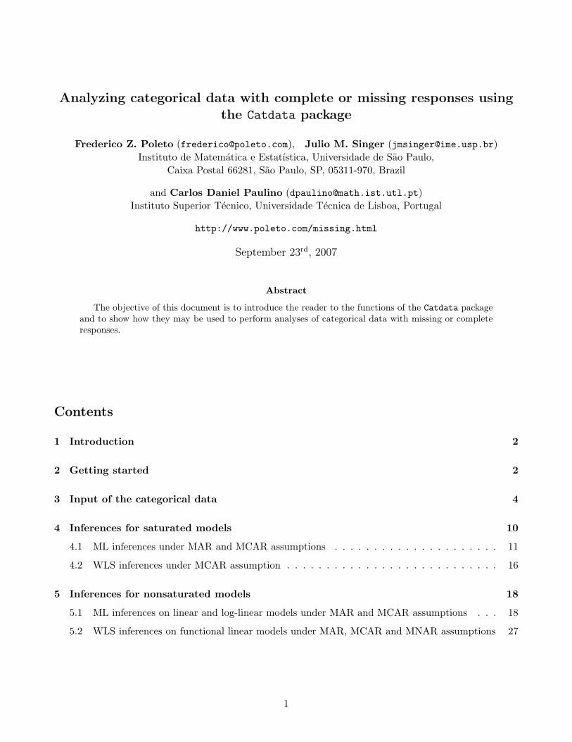
Freeman and Koch, 1976) or SAS’ PROC CATMOD. Figure 1 shows an outline of the analyses that may
be conducted by the library of functions.
The underlying theory is described in Poleto, Singer and Paulino (2007). We strongly recommend to
download this technical report from http://www.poleto.com/missing.html. It describes the statistical
theory, the notation, the examples, and also the models that will be analyzed.
In Section 2, we explain how to load Catdata and we give a brief overview of the functions included.
In Section 3, we show how to input the categorical data and the missingness patterns. In Sections 4
and 5, we illustrate the analysis of saturated and nonsaturated models for the marginal probabilities of
categorization.
2 Getting started
We intend to document all the functions and submit them as a contributed package to The Compre-
hensive R Archive Network (http://cran.r-project.org). In the meantime, the source code for the
functions may be loaded inside R using the command source("http://www.poleto.com/Catdata.r").
It is also possible to download the file from this site and load it using the source() command, specifying
where the file was saved and its label.
We describe, briefly, each of the functions:
• readCatdata() inputs the categorical data; it accommodates complete or missing data;
2
Possibleinputs:
Completedata
?> =<89 :;Observeddata and
missingnesspatterns
?> =<
89 :;
ttttttttttttt
θ and Vθ
(e.g., under aMNAR mechanism)
?> =<89 :;
Missingnessmechanism: MAR/. -,() *+ MCAR/. -,() *+
rrrrrrrrrrrrrrrrr
Inference onsaturated
models for θ:ML/. -,() *+
UUUUUUUUUUUUUUUUUUUUUUUUUUUUUUUUUUU WLS/. -,() *+
LLLLLLLLLLLLLLLLLL
Inference onnonsaturatedmodels for θ:
ML/. -,() *+
NNNNNNNNNNNNNNNN WLS/. -,() *+
Models: linear/. -,() *+ log-linear76 5401 23
qqqqqqqqqqqfunctional linear/. -,() *+
Goodness-of-fittests:
Likelihood ratio,Pearson, Waldand Neyman
?> =<89 :;
JJJJJJJJJJJJJ
Wald/. -,() *+
sssssssssssssssssss
Hypothesistests for theparameters:
Wald/. -,() *+
Figure 1: Analyses that can be conducted by the library of functions
• satMarML() generates the ML inference for saturated models under the MAR and MCAR mecha-
nisms based in a readCatdata() object; thus it can only be used in the context of missing data;
• satMcarWLS() generates the WLS inference for saturated models under the MCAR mechanism
based in a readCatdata() object; thus it can only be used in the context of missing data;
• linML() fits linear models by ML based in a readCatdata() object for complete data, or satMarML()
object for missing data;
• loglinML() fits log-linear models by ML based in a readCatdata() object for complete data, or
satMarML() object for missing data;
• funlinWLS() fits functional linear models by WLS based in a readCatdata() object for complete
data, satMarML() or satMcarWLS() objects for missing data, or based in estimates of the proba-
bilities of categorization and its consistent estimated covariance matrix obtained, for example, by
3
one of the built-in nonlinear optimization functions of R under any missingness mechanism or even
other kinds of models for the categorization probabilities;
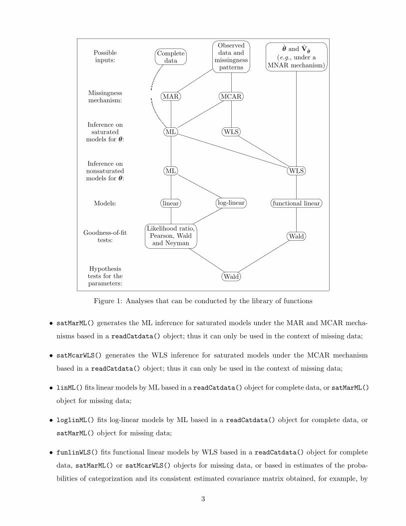
• waldTest() performs Wald tests in linML(), loglinML() and funlinWLS() objects, when the
models are expressed as freedom equations (Koch, Imrey, Singer, Atkinson and Stokes, 1985).
Figure 2 depicts the hierarchy of the usage of the functions.
readCatdata()missing data
completedata
nonlinearoptimization
functions
__ _ _ _ _ ����
����
_ _ _ _ __
satMarML() satMcarWLS()
linML() loglinML() funlinWLS()
waldTest()
Figure 2: Hierarchy of usage of the functions
3 Input of the categorical data
The categorical data input is accomplished with the function readCatdata(). The unique argument
to be informed in the case of complete data is TF, where the user must specify the table of frequencies.
TF may receive a vector, representing only one population (it assumes a multinomial distribution), or a
matrix, with each row representing one subpopulation (it assumes a product-multinomial distribution).
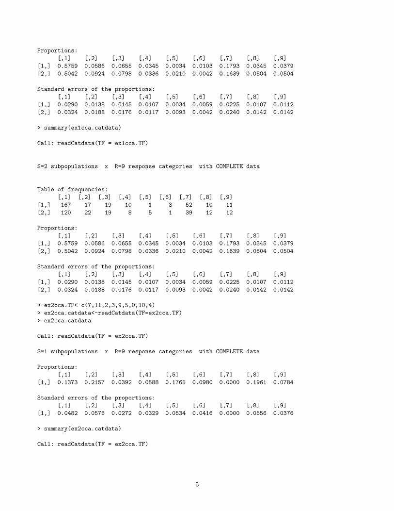
For instance, let us first disregard the missing data of the Examples 1 and 2 of Poleto et al. (2007) and
read only the complete data.
> ex1cca.TF<-rbind(c(167,17,19,10,1,3,52,10,11),+ c(120,22,19, 8,5,1,39,12,12))> ex1cca.catdata<-readCatdata(TF=ex1cca.TF)> ex1cca.catdata
Call: readCatdata(TF = ex1cca.TF)
S=2 subpopulations x R=9 response categories with COMPLETE data
4
Proportions:[,1] [,2] [,3] [,4] [,5] [,6] [,7] [,8] [,9]
[1,] 0.5759 0.0586 0.0655 0.0345 0.0034 0.0103 0.1793 0.0345 0.0379[2,] 0.5042 0.0924 0.0798 0.0336 0.0210 0.0042 0.1639 0.0504 0.0504
Standard errors of the proportions:[,1] [,2] [,3] [,4] [,5] [,6] [,7] [,8] [,9]
[1,] 0.0290 0.0138 0.0145 0.0107 0.0034 0.0059 0.0225 0.0107 0.0112[2,] 0.0324 0.0188 0.0176 0.0117 0.0093 0.0042 0.0240 0.0142 0.0142
> summary(ex1cca.catdata)
Call: readCatdata(TF = ex1cca.TF)
S=2 subpopulations x R=9 response categories with COMPLETE data
Table of frequencies:[,1] [,2] [,3] [,4] [,5] [,6] [,7] [,8] [,9]
[1,] 167 17 19 10 1 3 52 10 11[2,] 120 22 19 8 5 1 39 12 12
Proportions:[,1] [,2] [,3] [,4] [,5] [,6] [,7] [,8] [,9]
[1,] 0.5759 0.0586 0.0655 0.0345 0.0034 0.0103 0.1793 0.0345 0.0379[2,] 0.5042 0.0924 0.0798 0.0336 0.0210 0.0042 0.1639 0.0504 0.0504
Standard errors of the proportions:[,1] [,2] [,3] [,4] [,5] [,6] [,7] [,8] [,9]
[1,] 0.0290 0.0138 0.0145 0.0107 0.0034 0.0059 0.0225 0.0107 0.0112[2,] 0.0324 0.0188 0.0176 0.0117 0.0093 0.0042 0.0240 0.0142 0.0142
> ex2cca.TF<-c(7,11,2,3,9,5,0,10,4)> ex2cca.catdata<-readCatdata(TF=ex2cca.TF)> ex2cca.catdata
Call: readCatdata(TF = ex2cca.TF)
S=1 subpopulations x R=9 response categories with COMPLETE data
Proportions:[,1] [,2] [,3] [,4] [,5] [,6] [,7] [,8] [,9]
[1,] 0.1373 0.2157 0.0392 0.0588 0.1765 0.0980 0.0000 0.1961 0.0784
Standard errors of the proportions:[,1] [,2] [,3] [,4] [,5] [,6] [,7] [,8] [,9]
[1,] 0.0482 0.0576 0.0272 0.0329 0.0534 0.0416 0.0000 0.0556 0.0376
> summary(ex2cca.catdata)
Call: readCatdata(TF = ex2cca.TF)
5
S=1 subpopulations x R=9 response categories with COMPLETE data
Table of frequencies:[1] 7 11 2 3 9 5 0 10 4
Proportions:[,1] [,2] [,3] [,4] [,5] [,6] [,7] [,8] [,9]
[1,] 0.1373 0.2157 0.0392 0.0588 0.1765 0.0980 0.0000 0.1961 0.0784
Standard errors of the proportions:[,1] [,2] [,3] [,4] [,5] [,6] [,7] [,8] [,9]
[1,] 0.0482 0.0576 0.0272 0.0329 0.0534 0.0416 0.0000 0.0556 0.0376
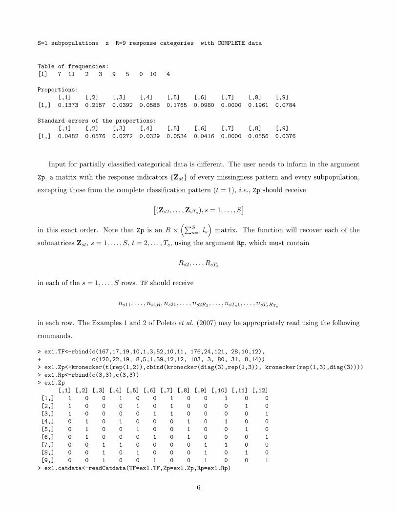
Input for partially classified categorical data is different. The user needs to inform in the argument
Zp, a matrix with the response indicators {Zst} of every missingness pattern and every subpopulation,
excepting those from the complete classification pattern (t = 1), i.e., Zp should receive
[(Zs2, . . . ,ZsTs), s = 1, . . . , S
]in this exact order. Note that Zp is an R ×
(∑Ss=1 ls
)matrix. The function will recover each of the
submatrices Zst, s = 1, . . . , S, t = 2, . . . , Ts, using the argument Rp, which must contain
Rs2, . . . , RsTs
in each of the s = 1, . . . , S rows. TF should receive
ns11, . . . , ns1R, ns21, . . . , ns2R2 , . . . , nsTs1, . . . , nsTsRTs
in each row. The Examples 1 and 2 of Poleto et al. (2007) may be appropriately read using the following
commands.
> ex1.TF<-rbind(c(167,17,19,10,1,3,52,10,11, 176,24,121, 28,10,12),+ c(120,22,19, 8,5,1,39,12,12, 103, 3, 80, 31, 8,14))> ex1.Zp<-kronecker(t(rep(1,2)),cbind(kronecker(diag(3),rep(1,3)), kronecker(rep(1,3),diag(3))))> ex1.Rp<-rbind(c(3,3),c(3,3))> ex1.Zp
[,1] [,2] [,3] [,4] [,5] [,6] [,7] [,8] [,9] [,10] [,11] [,12][1,] 1 0 0 1 0 0 1 0 0 1 0 0[2,] 1 0 0 0 1 0 1 0 0 0 1 0[3,] 1 0 0 0 0 1 1 0 0 0 0 1[4,] 0 1 0 1 0 0 0 1 0 1 0 0[5,] 0 1 0 0 1 0 0 1 0 0 1 0[6,] 0 1 0 0 0 1 0 1 0 0 0 1[7,] 0 0 1 1 0 0 0 0 1 1 0 0[8,] 0 0 1 0 1 0 0 0 1 0 1 0[9,] 0 0 1 0 0 1 0 0 1 0 0 1> ex1.catdata<-readCatdata(TF=ex1.TF,Zp=ex1.Zp,Rp=ex1.Rp)
6
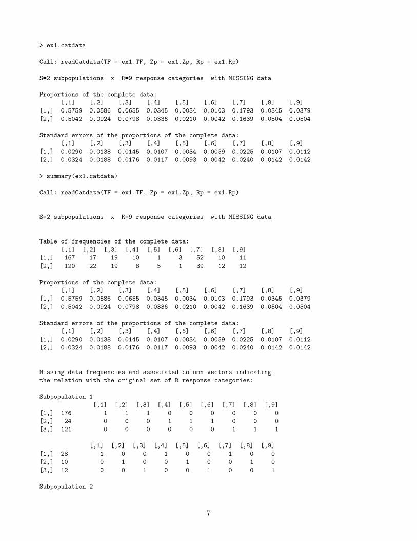
> ex1.catdata
Call: readCatdata(TF = ex1.TF, Zp = ex1.Zp, Rp = ex1.Rp)
S=2 subpopulations x R=9 response categories with MISSING data
Proportions of the complete data:[,1] [,2] [,3] [,4] [,5] [,6] [,7] [,8] [,9]
[1,] 0.5759 0.0586 0.0655 0.0345 0.0034 0.0103 0.1793 0.0345 0.0379[2,] 0.5042 0.0924 0.0798 0.0336 0.0210 0.0042 0.1639 0.0504 0.0504
Standard errors of the proportions of the complete data:[,1] [,2] [,3] [,4] [,5] [,6] [,7] [,8] [,9]
[1,] 0.0290 0.0138 0.0145 0.0107 0.0034 0.0059 0.0225 0.0107 0.0112[2,] 0.0324 0.0188 0.0176 0.0117 0.0093 0.0042 0.0240 0.0142 0.0142
> summary(ex1.catdata)
Call: readCatdata(TF = ex1.TF, Zp = ex1.Zp, Rp = ex1.Rp)
S=2 subpopulations x R=9 response categories with MISSING data
Table of frequencies of the complete data:[,1] [,2] [,3] [,4] [,5] [,6] [,7] [,8] [,9]
[1,] 167 17 19 10 1 3 52 10 11[2,] 120 22 19 8 5 1 39 12 12
Proportions of the complete data:[,1] [,2] [,3] [,4] [,5] [,6] [,7] [,8] [,9]
[1,] 0.5759 0.0586 0.0655 0.0345 0.0034 0.0103 0.1793 0.0345 0.0379[2,] 0.5042 0.0924 0.0798 0.0336 0.0210 0.0042 0.1639 0.0504 0.0504
Standard errors of the proportions of the complete data:[,1] [,2] [,3] [,4] [,5] [,6] [,7] [,8] [,9]
[1,] 0.0290 0.0138 0.0145 0.0107 0.0034 0.0059 0.0225 0.0107 0.0112[2,] 0.0324 0.0188 0.0176 0.0117 0.0093 0.0042 0.0240 0.0142 0.0142
Missing data frequencies and associated column vectors indicatingthe relation with the original set of R response categories:
Subpopulation 1[,1] [,2] [,3] [,4] [,5] [,6] [,7] [,8] [,9]
[1,] 176 1 1 1 0 0 0 0 0 0[2,] 24 0 0 0 1 1 1 0 0 0[3,] 121 0 0 0 0 0 0 1 1 1
[,1] [,2] [,3] [,4] [,5] [,6] [,7] [,8] [,9][1,] 28 1 0 0 1 0 0 1 0 0[2,] 10 0 1 0 0 1 0 0 1 0[3,] 12 0 0 1 0 0 1 0 0 1
Subpopulation 2
7
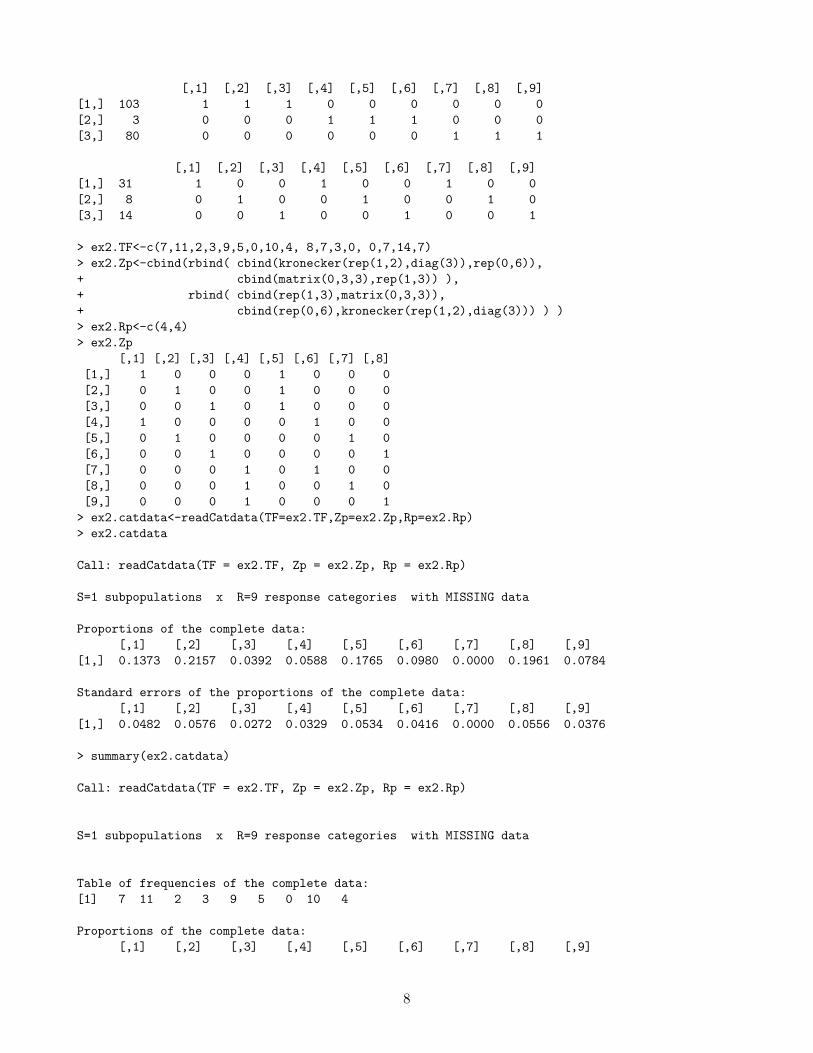
[,1] [,2] [,3] [,4] [,5] [,6] [,7] [,8] [,9][1,] 103 1 1 1 0 0 0 0 0 0[2,] 3 0 0 0 1 1 1 0 0 0[3,] 80 0 0 0 0 0 0 1 1 1
[,1] [,2] [,3] [,4] [,5] [,6] [,7] [,8] [,9][1,] 31 1 0 0 1 0 0 1 0 0[2,] 8 0 1 0 0 1 0 0 1 0[3,] 14 0 0 1 0 0 1 0 0 1
> ex2.TF<-c(7,11,2,3,9,5,0,10,4, 8,7,3,0, 0,7,14,7)> ex2.Zp<-cbind(rbind( cbind(kronecker(rep(1,2),diag(3)),rep(0,6)),+ cbind(matrix(0,3,3),rep(1,3)) ),+ rbind( cbind(rep(1,3),matrix(0,3,3)),+ cbind(rep(0,6),kronecker(rep(1,2),diag(3))) ) )> ex2.Rp<-c(4,4)> ex2.Zp
[,1] [,2] [,3] [,4] [,5] [,6] [,7] [,8][1,] 1 0 0 0 1 0 0 0[2,] 0 1 0 0 1 0 0 0[3,] 0 0 1 0 1 0 0 0[4,] 1 0 0 0 0 1 0 0[5,] 0 1 0 0 0 0 1 0[6,] 0 0 1 0 0 0 0 1[7,] 0 0 0 1 0 1 0 0[8,] 0 0 0 1 0 0 1 0[9,] 0 0 0 1 0 0 0 1> ex2.catdata<-readCatdata(TF=ex2.TF,Zp=ex2.Zp,Rp=ex2.Rp)> ex2.catdata
Call: readCatdata(TF = ex2.TF, Zp = ex2.Zp, Rp = ex2.Rp)
S=1 subpopulations x R=9 response categories with MISSING data
Proportions of the complete data:[,1] [,2] [,3] [,4] [,5] [,6] [,7] [,8] [,9]
[1,] 0.1373 0.2157 0.0392 0.0588 0.1765 0.0980 0.0000 0.1961 0.0784
Standard errors of the proportions of the complete data:[,1] [,2] [,3] [,4] [,5] [,6] [,7] [,8] [,9]
[1,] 0.0482 0.0576 0.0272 0.0329 0.0534 0.0416 0.0000 0.0556 0.0376
> summary(ex2.catdata)
Call: readCatdata(TF = ex2.TF, Zp = ex2.Zp, Rp = ex2.Rp)
S=1 subpopulations x R=9 response categories with MISSING data
Table of frequencies of the complete data:[1] 7 11 2 3 9 5 0 10 4
Proportions of the complete data:[,1] [,2] [,3] [,4] [,5] [,6] [,7] [,8] [,9]
8
[1,] 0.1373 0.2157 0.0392 0.0588 0.1765 0.0980 0.0000 0.1961 0.0784
Standard errors of the proportions of the complete data:[,1] [,2] [,3] [,4] [,5] [,6] [,7] [,8] [,9]
[1,] 0.0482 0.0576 0.0272 0.0329 0.0534 0.0416 0.0000 0.0556 0.0376
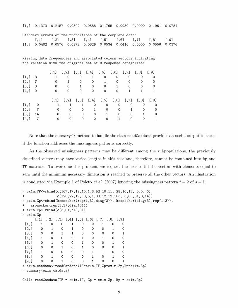
Missing data frequencies and associated column vectors indicatingthe relation with the original set of R response categories:
[,1] [,2] [,3] [,4] [,5] [,6] [,7] [,8] [,9][1,] 8 1 0 0 1 0 0 0 0 0[2,] 7 0 1 0 0 1 0 0 0 0[3,] 3 0 0 1 0 0 1 0 0 0[4,] 0 0 0 0 0 0 0 1 1 1
[,1] [,2] [,3] [,4] [,5] [,6] [,7] [,8] [,9][1,] 0 1 1 1 0 0 0 0 0 0[2,] 7 0 0 0 1 0 0 1 0 0[3,] 14 0 0 0 0 1 0 0 1 0[4,] 7 0 0 0 0 0 1 0 0 1
Note that the summary() method to handle the class readCatdata provides an useful output to check
if the function addresses the missingness patterns correctly.
As the observed missingness patterns may be different among the subpopulations, the previously
described vectors may have varied lengths in this case and, therefore, cannot be combined into Rp and
TF matrices. To overcome this problem, we request the user to fill the vectors with elements equal to
zero until the minimum necessary dimension is reached to preserve all the other vectors. An illustration
is conducted via Example 1 of Poleto et al. (2007) ignoring the missingness pattern t = 2 of s = 1.
> ex1m.TF<-rbind(c(167,17,19,10,1,3,52,10,11, 28,10,12, 0,0, 0),+ c(120,22,19, 8,5,1,39,12,12,103, 3,80,31,8,14))> ex1m.Zp<-cbind(kronecker(rep(1,3),diag(3)), kronecker(diag(3),rep(1,3)),+ kronecker(rep(1,3),diag(3)))> ex1m.Rp<-rbind(c(3,0),c(3,3))> ex1m.Zp
[,1] [,2] [,3] [,4] [,5] [,6] [,7] [,8] [,9][1,] 1 0 0 1 0 0 1 0 0[2,] 0 1 0 1 0 0 0 1 0[3,] 0 0 1 1 0 0 0 0 1[4,] 1 0 0 0 1 0 1 0 0[5,] 0 1 0 0 1 0 0 1 0[6,] 0 0 1 0 1 0 0 0 1[7,] 1 0 0 0 0 1 1 0 0[8,] 0 1 0 0 0 1 0 1 0[9,] 0 0 1 0 0 1 0 0 1> ex1m.catdata<-readCatdata(TF=ex1m.TF,Zp=ex1m.Zp,Rp=ex1m.Rp)> summary(ex1m.catdata)
Call: readCatdata(TF = ex1m.TF, Zp = ex1m.Zp, Rp = ex1m.Rp)
9
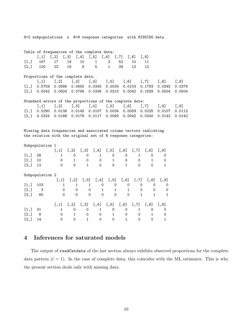
S=2 subpopulations x R=9 response categories with MISSING data
Table of frequencies of the complete data:[,1] [,2] [,3] [,4] [,5] [,6] [,7] [,8] [,9]
[1,] 167 17 19 10 1 3 52 10 11[2,] 120 22 19 8 5 1 39 12 12
Proportions of the complete data:[,1] [,2] [,3] [,4] [,5] [,6] [,7] [,8] [,9]
[1,] 0.5759 0.0586 0.0655 0.0345 0.0034 0.0103 0.1793 0.0345 0.0379[2,] 0.5042 0.0924 0.0798 0.0336 0.0210 0.0042 0.1639 0.0504 0.0504
Standard errors of the proportions of the complete data:[,1] [,2] [,3] [,4] [,5] [,6] [,7] [,8] [,9]
[1,] 0.0290 0.0138 0.0145 0.0107 0.0034 0.0059 0.0225 0.0107 0.0112[2,] 0.0324 0.0188 0.0176 0.0117 0.0093 0.0042 0.0240 0.0142 0.0142
Missing data frequencies and associated column vectors indicatingthe relation with the original set of R response categories:
Subpopulation 1[,1] [,2] [,3] [,4] [,5] [,6] [,7] [,8] [,9]
[1,] 28 1 0 0 1 0 0 1 0 0[2,] 10 0 1 0 0 1 0 0 1 0[3,] 12 0 0 1 0 0 1 0 0 1
Subpopulation 2[,1] [,2] [,3] [,4] [,5] [,6] [,7] [,8] [,9]
[1,] 103 1 1 1 0 0 0 0 0 0[2,] 3 0 0 0 1 1 1 0 0 0[3,] 80 0 0 0 0 0 0 1 1 1
[,1] [,2] [,3] [,4] [,5] [,6] [,7] [,8] [,9][1,] 31 1 0 0 1 0 0 1 0 0[2,] 8 0 1 0 0 1 0 0 1 0[3,] 14 0 0 1 0 0 1 0 0 1
4 Inferences for saturated models
The output of readCatdata of the last section always exhibits observed proportions for the complete
data pattern (t = 1). In the case of complete data, this coincides with the ML estimates. This is why
the present section deals only with missing data.
10
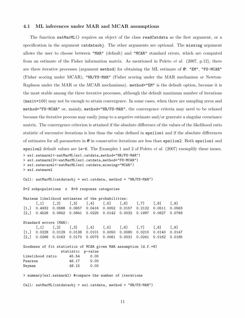
4.1 ML inferences under MAR and MCAR assumptions
The function satMarML() requires an object of the class readCatdata as the first argument, or a
specification in the argument catdataobj. The other arguments are optional. The missing argument
allows the user to choose between "MAR" (default) and "MCAR" standard errors, which are computed
from an estimate of the Fisher information matrix. As mentioned in Poleto et al. (2007, p.12), there
are three iterative processes (argument method) for obtaining the ML estimate of θ: "EM", "FS-MCAR"
(Fisher scoring under MCAR), "NR/FS-MAR" (Fisher scoring under the MAR mechanism or Newton-
Raphson under the MAR or the MCAR mechanisms). method="EM" is the default option, because it is
the most stable among the three iterative processes, although the default maximum number of iterations
(maxit=100) may not be enough to attain convergence. In some cases, when there are sampling zeros and
method="FS-MCAR" or, mainly, method="NR/FS-MAR", the convergence criteria may need to be relaxed
because the iterative process may easily jump to a negative estimate and/or generate a singular covariance
matrix. The convergence criterion is attained if the absolute difference of the values of the likelihood ratio
statistic of successive iterations is less than the value defined in epsilon1 and if the absolute differences
of estimates for all parameters in θ in consecutive iterations are less than epsilon2. Both epsilon1 and
epsilon2 default values are 1e-6. The Examples 1 and 2 of Poleto et al. (2007) exemplify these issues.> ex1.satmarml<-satMarML(ex1.catdata,method="NR/FS-MAR")> ex1.satmarml2<-satMarML(ex1.catdata,method="FS-MCAR")> ex1.satmcarml<-satMarML(ex1.catdata,missing="MCAR")> ex1.satmarml
Call: satMarML(catdataobj = ex1.catdata, method = "NR/FS-MAR")
S=2 subpopulations x R=9 response categories
Maximum likelihood estimates of the probabilities:[,1] [,2] [,3] [,4] [,5] [,6] [,7] [,8] [,9]
[1,] 0.4932 0.0588 0.0657 0.0416 0.0052 0.0157 0.2122 0.0511 0.0563[2,] 0.4526 0.0842 0.0841 0.0225 0.0142 0.0032 0.1997 0.0627 0.0769
Standard errors (MAR):[,1] [,2] [,3] [,4] [,5] [,6] [,7] [,8] [,9]
[1,] 0.0228 0.0129 0.0136 0.0101 0.0050 0.0080 0.0210 0.0140 0.0147[2,] 0.0266 0.0163 0.0170 0.0075 0.0061 0.0031 0.0241 0.0162 0.0185
Goodness of fit statistics of MCAR given MAR assumption (d.f.=8)statistic p-value
Likelihood ratio 45.54 0.00Pearson 46.17 0.00Neyman 48.15 0.00
> summary(ex1.satmarml) #compare the number of iterations
Call: satMarML(catdataobj = ex1.catdata, method = "NR/FS-MAR")
11
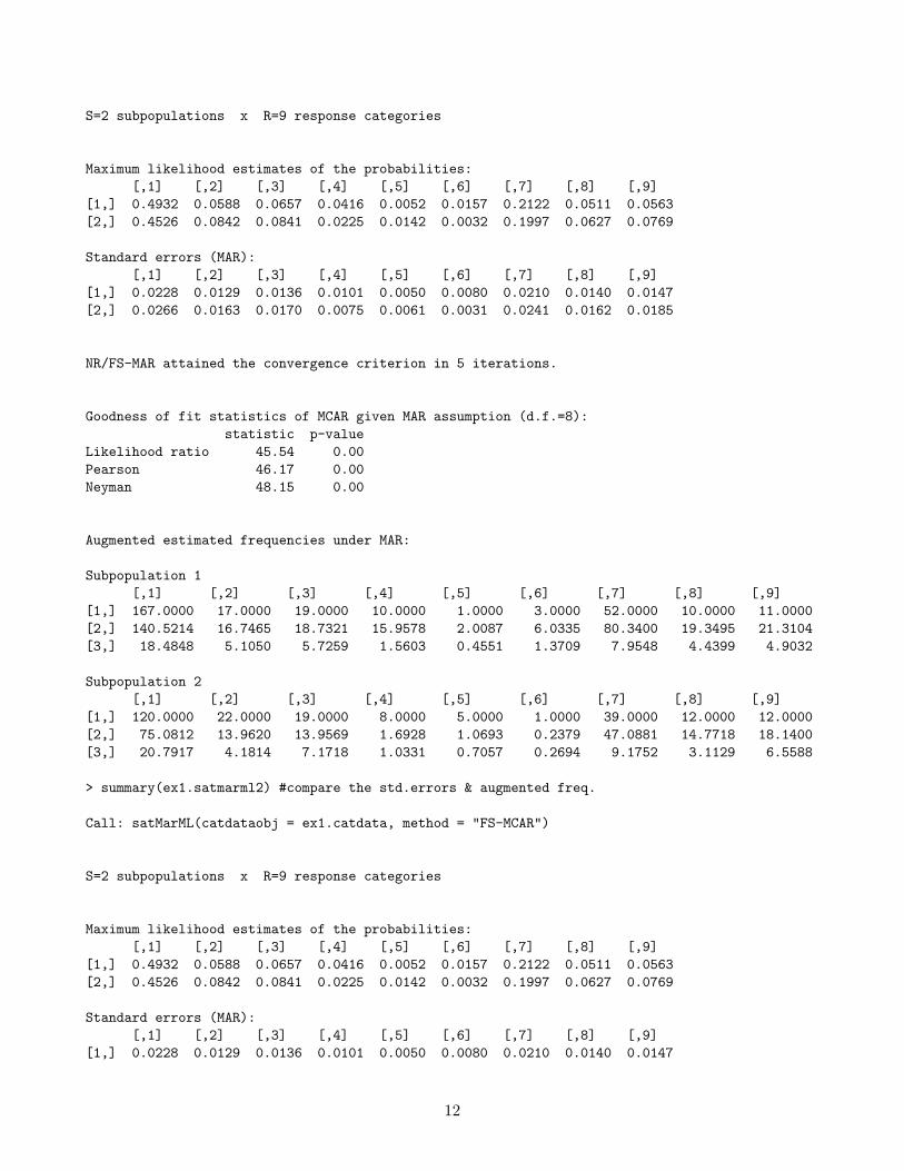
S=2 subpopulations x R=9 response categories
Maximum likelihood estimates of the probabilities:[,1] [,2] [,3] [,4] [,5] [,6] [,7] [,8] [,9]
[1,] 0.4932 0.0588 0.0657 0.0416 0.0052 0.0157 0.2122 0.0511 0.0563[2,] 0.4526 0.0842 0.0841 0.0225 0.0142 0.0032 0.1997 0.0627 0.0769
Standard errors (MAR):[,1] [,2] [,3] [,4] [,5] [,6] [,7] [,8] [,9]
[1,] 0.0228 0.0129 0.0136 0.0101 0.0050 0.0080 0.0210 0.0140 0.0147[2,] 0.0266 0.0163 0.0170 0.0075 0.0061 0.0031 0.0241 0.0162 0.0185
NR/FS-MAR attained the convergence criterion in 5 iterations.
Goodness of fit statistics of MCAR given MAR assumption (d.f.=8):statistic p-value
Likelihood ratio 45.54 0.00Pearson 46.17 0.00Neyman 48.15 0.00
Augmented estimated frequencies under MAR:
Subpopulation 1[,1] [,2] [,3] [,4] [,5] [,6] [,7] [,8] [,9]
[1,] 167.0000 17.0000 19.0000 10.0000 1.0000 3.0000 52.0000 10.0000 11.0000[2,] 140.5214 16.7465 18.7321 15.9578 2.0087 6.0335 80.3400 19.3495 21.3104[3,] 18.4848 5.1050 5.7259 1.5603 0.4551 1.3709 7.9548 4.4399 4.9032
Subpopulation 2[,1] [,2] [,3] [,4] [,5] [,6] [,7] [,8] [,9]
[1,] 120.0000 22.0000 19.0000 8.0000 5.0000 1.0000 39.0000 12.0000 12.0000[2,] 75.0812 13.9620 13.9569 1.6928 1.0693 0.2379 47.0881 14.7718 18.1400[3,] 20.7917 4.1814 7.1718 1.0331 0.7057 0.2694 9.1752 3.1129 6.5588
> summary(ex1.satmarml2) #compare the std.errors & augmented freq.
Call: satMarML(catdataobj = ex1.catdata, method = "FS-MCAR")
S=2 subpopulations x R=9 response categories
Maximum likelihood estimates of the probabilities:[,1] [,2] [,3] [,4] [,5] [,6] [,7] [,8] [,9]
[1,] 0.4932 0.0588 0.0657 0.0416 0.0052 0.0157 0.2122 0.0511 0.0563[2,] 0.4526 0.0842 0.0841 0.0225 0.0142 0.0032 0.1997 0.0627 0.0769
Standard errors (MAR):[,1] [,2] [,3] [,4] [,5] [,6] [,7] [,8] [,9]
[1,] 0.0228 0.0129 0.0136 0.0101 0.0050 0.0080 0.0210 0.0140 0.0147
12
[2,] 0.0266 0.0163 0.0170 0.0075 0.0061 0.0031 0.0241 0.0162 0.0185
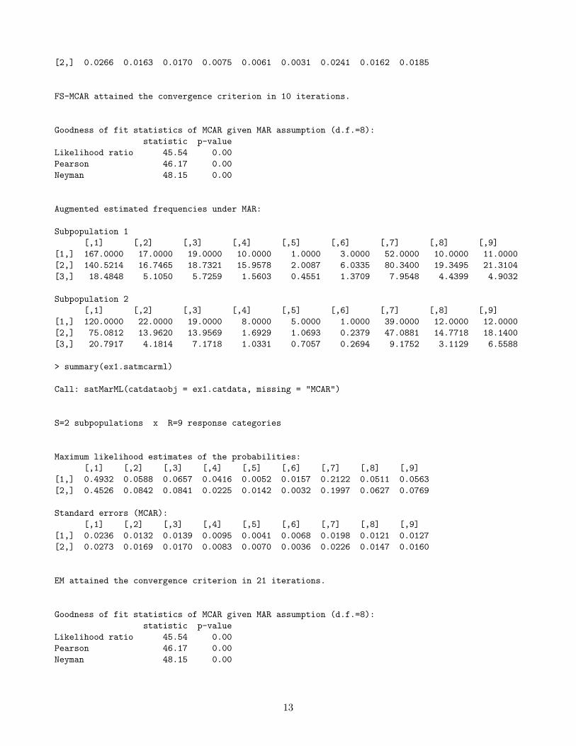
FS-MCAR attained the convergence criterion in 10 iterations.
Goodness of fit statistics of MCAR given MAR assumption (d.f.=8):statistic p-value
Likelihood ratio 45.54 0.00Pearson 46.17 0.00Neyman 48.15 0.00
Augmented estimated frequencies under MAR:
Subpopulation 1[,1] [,2] [,3] [,4] [,5] [,6] [,7] [,8] [,9]
[1,] 167.0000 17.0000 19.0000 10.0000 1.0000 3.0000 52.0000 10.0000 11.0000[2,] 140.5214 16.7465 18.7321 15.9578 2.0087 6.0335 80.3400 19.3495 21.3104[3,] 18.4848 5.1050 5.7259 1.5603 0.4551 1.3709 7.9548 4.4399 4.9032
Subpopulation 2[,1] [,2] [,3] [,4] [,5] [,6] [,7] [,8] [,9]
[1,] 120.0000 22.0000 19.0000 8.0000 5.0000 1.0000 39.0000 12.0000 12.0000[2,] 75.0812 13.9620 13.9569 1.6929 1.0693 0.2379 47.0881 14.7718 18.1400[3,] 20.7917 4.1814 7.1718 1.0331 0.7057 0.2694 9.1752 3.1129 6.5588
> summary(ex1.satmcarml)
Call: satMarML(catdataobj = ex1.catdata, missing = "MCAR")
S=2 subpopulations x R=9 response categories
Maximum likelihood estimates of the probabilities:[,1] [,2] [,3] [,4] [,5] [,6] [,7] [,8] [,9]
[1,] 0.4932 0.0588 0.0657 0.0416 0.0052 0.0157 0.2122 0.0511 0.0563[2,] 0.4526 0.0842 0.0841 0.0225 0.0142 0.0032 0.1997 0.0627 0.0769
Standard errors (MCAR):[,1] [,2] [,3] [,4] [,5] [,6] [,7] [,8] [,9]
[1,] 0.0236 0.0132 0.0139 0.0095 0.0041 0.0068 0.0198 0.0121 0.0127[2,] 0.0273 0.0169 0.0170 0.0083 0.0070 0.0036 0.0226 0.0147 0.0160
EM attained the convergence criterion in 21 iterations.
Goodness of fit statistics of MCAR given MAR assumption (d.f.=8):statistic p-value
Likelihood ratio 45.54 0.00Pearson 46.17 0.00Neyman 48.15 0.00
13
Augmented estimated frequencies under MCAR:
Subpopulation 1[,1] [,2] [,3] [,4] [,5] [,6] [,7] [,8] [,9]
[1,] 143.028 17.045 19.066 12.073 1.520 4.565 61.552 14.824 16.326[2,] 158.317 18.867 21.105 13.364 1.682 5.053 68.132 16.409 18.072[3,] 24.660 2.939 3.287 2.082 0.262 0.787 10.612 2.556 2.815
Subpopulation 2[,1] [,2] [,3] [,4] [,5] [,6] [,7] [,8] [,9]
[1,] 107.7101 20.0296 20.0223 5.3517 3.3804 0.7521 47.5319 14.9110 18.3109[2,] 84.1768 15.6534 15.6477 4.1824 2.6418 0.5877 37.1468 11.6532 14.3102[3,] 23.9859 4.4604 4.4587 1.1918 0.7528 0.1675 10.5848 3.3205 4.0776
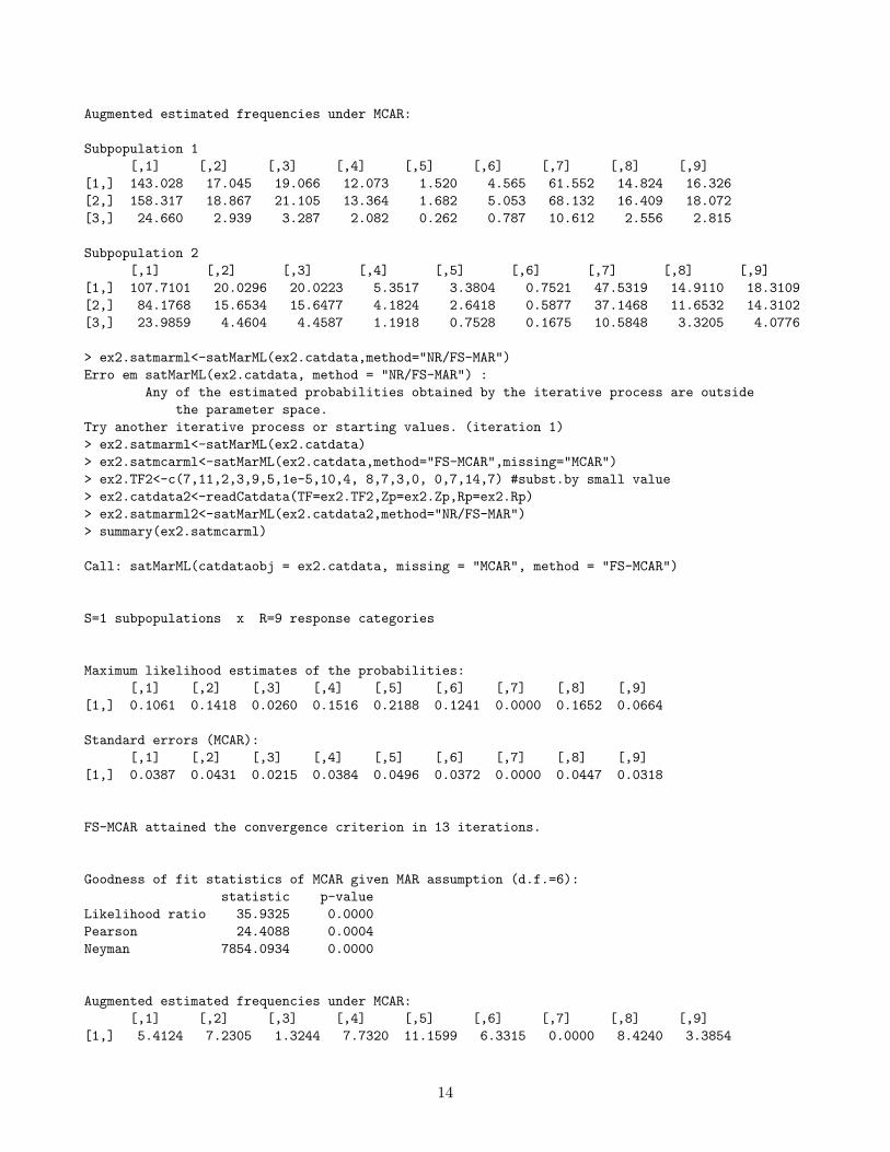
> ex2.satmarml<-satMarML(ex2.catdata,method="NR/FS-MAR")Erro em satMarML(ex2.catdata, method = "NR/FS-MAR") :
Any of the estimated probabilities obtained by the iterative process are outsidethe parameter space.
Try another iterative process or starting values. (iteration 1)> ex2.satmarml<-satMarML(ex2.catdata)> ex2.satmcarml<-satMarML(ex2.catdata,method="FS-MCAR",missing="MCAR")> ex2.TF2<-c(7,11,2,3,9,5,1e-5,10,4, 8,7,3,0, 0,7,14,7) #subst.by small value> ex2.catdata2<-readCatdata(TF=ex2.TF2,Zp=ex2.Zp,Rp=ex2.Rp)> ex2.satmarml2<-satMarML(ex2.catdata2,method="NR/FS-MAR")> summary(ex2.satmcarml)
Call: satMarML(catdataobj = ex2.catdata, missing = "MCAR", method = "FS-MCAR")
S=1 subpopulations x R=9 response categories
Maximum likelihood estimates of the probabilities:[,1] [,2] [,3] [,4] [,5] [,6] [,7] [,8] [,9]
[1,] 0.1061 0.1418 0.0260 0.1516 0.2188 0.1241 0.0000 0.1652 0.0664
Standard errors (MCAR):[,1] [,2] [,3] [,4] [,5] [,6] [,7] [,8] [,9]
[1,] 0.0387 0.0431 0.0215 0.0384 0.0496 0.0372 0.0000 0.0447 0.0318
FS-MCAR attained the convergence criterion in 13 iterations.
Goodness of fit statistics of MCAR given MAR assumption (d.f.=6):statistic p-value
Likelihood ratio 35.9325 0.0000Pearson 24.4088 0.0004Neyman 7854.0934 0.0000
Augmented estimated frequencies under MCAR:[,1] [,2] [,3] [,4] [,5] [,6] [,7] [,8] [,9]
[1,] 5.4124 7.2305 1.3244 7.7320 11.1599 6.3315 0.0000 8.4240 3.3854
14
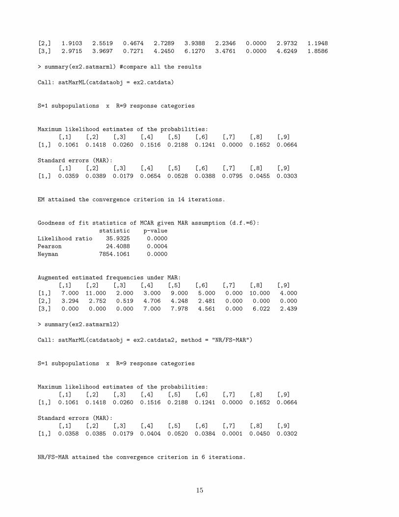
[2,] 1.9103 2.5519 0.4674 2.7289 3.9388 2.2346 0.0000 2.9732 1.1948[3,] 2.9715 3.9697 0.7271 4.2450 6.1270 3.4761 0.0000 4.6249 1.8586
> summary(ex2.satmarml) #compare all the results
Call: satMarML(catdataobj = ex2.catdata)
S=1 subpopulations x R=9 response categories
Maximum likelihood estimates of the probabilities:[,1] [,2] [,3] [,4] [,5] [,6] [,7] [,8] [,9]
[1,] 0.1061 0.1418 0.0260 0.1516 0.2188 0.1241 0.0000 0.1652 0.0664
Standard errors (MAR):[,1] [,2] [,3] [,4] [,5] [,6] [,7] [,8] [,9]
[1,] 0.0359 0.0389 0.0179 0.0654 0.0528 0.0388 0.0795 0.0455 0.0303
EM attained the convergence criterion in 14 iterations.
Goodness of fit statistics of MCAR given MAR assumption (d.f.=6):statistic p-value
Likelihood ratio 35.9325 0.0000Pearson 24.4088 0.0004Neyman 7854.1061 0.0000
Augmented estimated frequencies under MAR:[,1] [,2] [,3] [,4] [,5] [,6] [,7] [,8] [,9]
[1,] 7.000 11.000 2.000 3.000 9.000 5.000 0.000 10.000 4.000[2,] 3.294 2.752 0.519 4.706 4.248 2.481 0.000 0.000 0.000[3,] 0.000 0.000 0.000 7.000 7.978 4.561 0.000 6.022 2.439
> summary(ex2.satmarml2)
Call: satMarML(catdataobj = ex2.catdata2, method = "NR/FS-MAR")
S=1 subpopulations x R=9 response categories
Maximum likelihood estimates of the probabilities:[,1] [,2] [,3] [,4] [,5] [,6] [,7] [,8] [,9]
[1,] 0.1061 0.1418 0.0260 0.1516 0.2188 0.1241 0.0000 0.1652 0.0664
Standard errors (MAR):[,1] [,2] [,3] [,4] [,5] [,6] [,7] [,8] [,9]
[1,] 0.0358 0.0385 0.0179 0.0404 0.0520 0.0384 0.0001 0.0450 0.0302
NR/FS-MAR attained the convergence criterion in 6 iterations.
15
Goodness of fit statistics of MCAR given MAR assumption (d.f.=6):statistic p-value
Likelihood ratio 35.9325 0.0000Pearson 24.4088 0.0004Neyman 7854.0962 0.0000
Augmented estimated frequencies under MAR:[,1] [,2] [,3] [,4] [,5] [,6] [,7] [,8] [,9]
[1,] 7.000 11.000 2.000 3.000 9.000 5.000 0.000 10.000 4.000[2,] 3.294 2.752 0.519 4.706 4.248 2.481 0.000 0.000 0.000[3,] 0.000 0.000 0.000 7.000 7.978 4.561 0.000 6.022 2.439
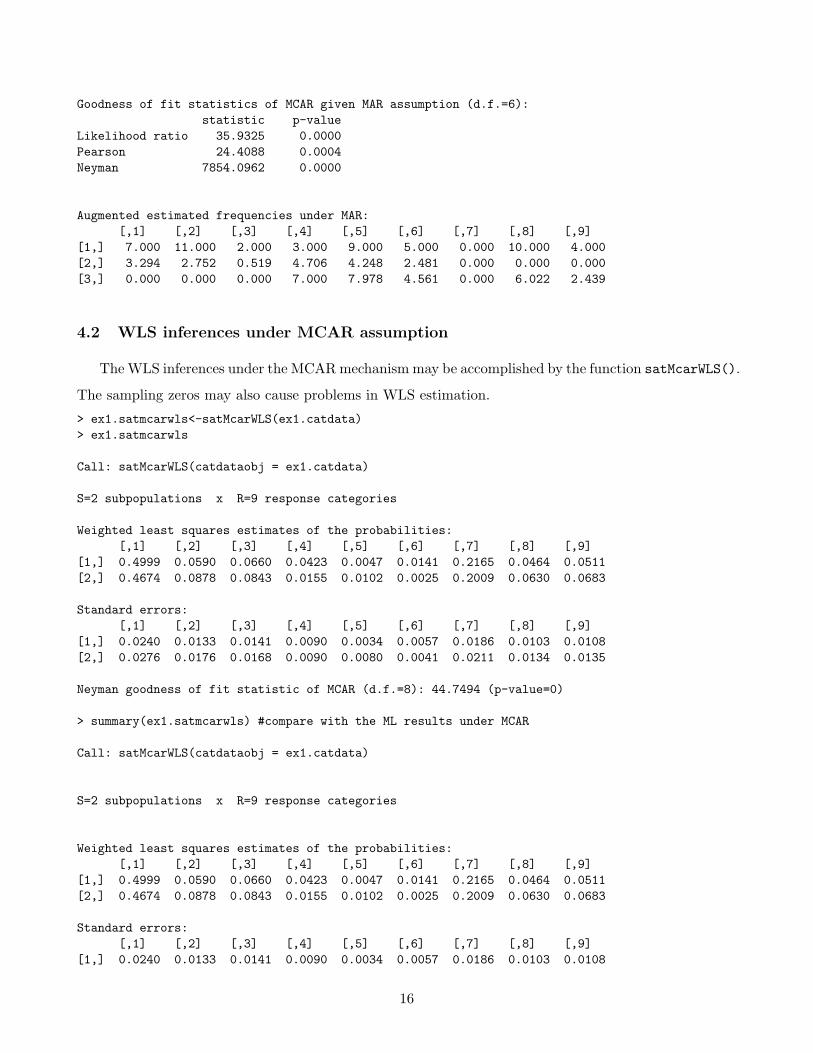
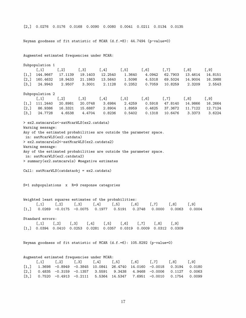
4.2 WLS inferences under MCAR assumption
The WLS inferences under the MCAR mechanism may be accomplished by the function satMcarWLS().
The sampling zeros may also cause problems in WLS estimation.
> ex1.satmcarwls<-satMcarWLS(ex1.catdata)> ex1.satmcarwls
Call: satMcarWLS(catdataobj = ex1.catdata)
S=2 subpopulations x R=9 response categories
Weighted least squares estimates of the probabilities:[,1] [,2] [,3] [,4] [,5] [,6] [,7] [,8] [,9]
[1,] 0.4999 0.0590 0.0660 0.0423 0.0047 0.0141 0.2165 0.0464 0.0511[2,] 0.4674 0.0878 0.0843 0.0155 0.0102 0.0025 0.2009 0.0630 0.0683
Standard errors:[,1] [,2] [,3] [,4] [,5] [,6] [,7] [,8] [,9]
[1,] 0.0240 0.0133 0.0141 0.0090 0.0034 0.0057 0.0186 0.0103 0.0108[2,] 0.0276 0.0176 0.0168 0.0090 0.0080 0.0041 0.0211 0.0134 0.0135
Neyman goodness of fit statistic of MCAR (d.f.=8): 44.7494 (p-value=0)
> summary(ex1.satmcarwls) #compare with the ML results under MCAR
Call: satMcarWLS(catdataobj = ex1.catdata)
S=2 subpopulations x R=9 response categories
Weighted least squares estimates of the probabilities:[,1] [,2] [,3] [,4] [,5] [,6] [,7] [,8] [,9]
[1,] 0.4999 0.0590 0.0660 0.0423 0.0047 0.0141 0.2165 0.0464 0.0511[2,] 0.4674 0.0878 0.0843 0.0155 0.0102 0.0025 0.2009 0.0630 0.0683
Standard errors:[,1] [,2] [,3] [,4] [,5] [,6] [,7] [,8] [,9]
[1,] 0.0240 0.0133 0.0141 0.0090 0.0034 0.0057 0.0186 0.0103 0.0108
16
[2,] 0.0276 0.0176 0.0168 0.0090 0.0080 0.0041 0.0211 0.0134 0.0135
Neyman goodness of fit statistic of MCAR (d.f.=8): 44.7494 (p-value=0)
Augmented estimated frequencies under MCAR:
Subpopulation 1[,1] [,2] [,3] [,4] [,5] [,6] [,7] [,8] [,9]
[1,] 144.9667 17.1139 19.1403 12.2540 1.3640 4.0942 62.7903 13.4614 14.8151[2,] 160.4632 18.9433 21.1863 13.5640 1.5098 4.5318 69.5024 14.9004 16.3988[3,] 24.9943 2.9507 3.3001 2.1128 0.2352 0.7059 10.8259 2.3209 2.5543
Subpopulation 2[,1] [,2] [,3] [,4] [,5] [,6] [,7] [,8] [,9]
[1,] 111.2440 20.8981 20.0748 3.6984 2.4259 0.5918 47.8140 14.9866 16.2664[2,] 86.9386 16.3321 15.6887 2.8904 1.8959 0.4625 37.3672 11.7122 12.7124[3,] 24.7728 4.6538 4.4704 0.8236 0.5402 0.1318 10.6476 3.3373 3.6224
> ex2.satmcarwls<-satMcarWLS(ex2.catdata)Warning message:Any of the estimated probabilities are outside the parameter space.in: satMcarWLS(ex2.catdata)> ex2.satmcarwls2<-satMcarWLS(ex2.catdata2)Warning message:Any of the estimated probabilities are outside the parameter space.in: satMcarWLS(ex2.catdata2)> summary(ex2.satmcarwls) #negative estimates
Call: satMcarWLS(catdataobj = ex2.catdata)
S=1 subpopulations x R=9 response categories
Weighted least squares estimates of the probabilities:[,1] [,2] [,3] [,4] [,5] [,6] [,7] [,8] [,9]
[1,] 0.0269 -0.0175 -0.0075 0.1977 0.5191 0.2748 0.0000 0.0063 0.0004
Standard errors:[,1] [,2] [,3] [,4] [,5] [,6] [,7] [,8] [,9]
[1,] 0.0394 0.0410 0.0253 0.0281 0.0357 0.0319 0.0009 0.0312 0.0309
Neyman goodness of fit statistic of MCAR (d.f.=6): 105.8292 (p-value=0)
Augmented estimated frequencies under MCAR:[,1] [,2] [,3] [,4] [,5] [,6] [,7] [,8] [,9]
[1,] 1.3698 -0.8949 -0.3845 10.0841 26.4740 14.0160 -0.0018 0.3194 0.0180[2,] 0.4835 -0.3159 -0.1357 3.5591 9.3438 4.9468 -0.0006 0.1127 0.0063[3,] 0.7520 -0.4913 -0.2111 5.5364 14.5347 7.6951 -0.0010 0.1754 0.0099
17
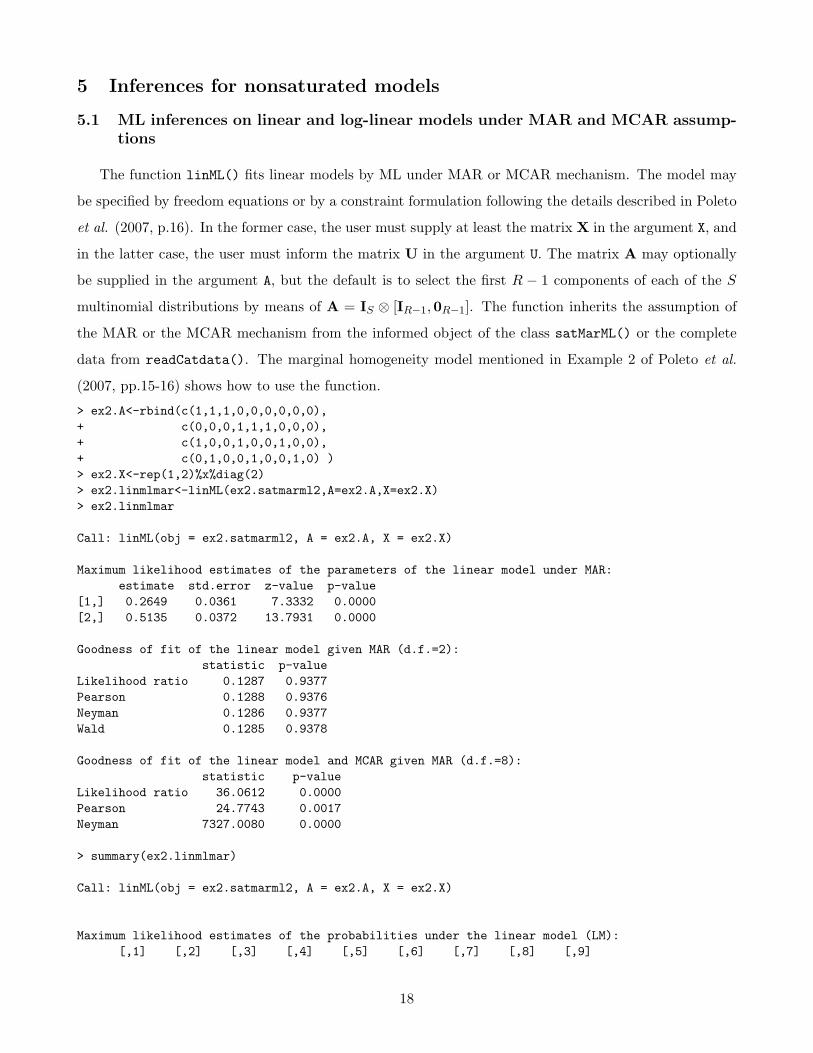
5 Inferences for nonsaturated models
5.1 ML inferences on linear and log-linear models under MAR and MCAR assump-tions
The function linML() fits linear models by ML under MAR or MCAR mechanism. The model may
be specified by freedom equations or by a constraint formulation following the details described in Poleto
et al. (2007, p.16). In the former case, the user must supply at least the matrix X in the argument X, and
in the latter case, the user must inform the matrix U in the argument U. The matrix A may optionally
be supplied in the argument A, but the default is to select the first R − 1 components of each of the S
multinomial distributions by means of A = IS ⊗ [IR−1,0R−1]. The function inherits the assumption of
the MAR or the MCAR mechanism from the informed object of the class satMarML() or the complete
data from readCatdata(). The marginal homogeneity model mentioned in Example 2 of Poleto et al.
(2007, pp.15-16) shows how to use the function.
> ex2.A<-rbind(c(1,1,1,0,0,0,0,0,0),+ c(0,0,0,1,1,1,0,0,0),+ c(1,0,0,1,0,0,1,0,0),+ c(0,1,0,0,1,0,0,1,0) )> ex2.X<-rep(1,2)%x%diag(2)> ex2.linmlmar<-linML(ex2.satmarml2,A=ex2.A,X=ex2.X)> ex2.linmlmar
Call: linML(obj = ex2.satmarml2, A = ex2.A, X = ex2.X)
Maximum likelihood estimates of the parameters of the linear model under MAR:estimate std.error z-value p-value
[1,] 0.2649 0.0361 7.3332 0.0000[2,] 0.5135 0.0372 13.7931 0.0000
Goodness of fit of the linear model given MAR (d.f.=2):statistic p-value
Likelihood ratio 0.1287 0.9377Pearson 0.1288 0.9376Neyman 0.1286 0.9377Wald 0.1285 0.9378
Goodness of fit of the linear model and MCAR given MAR (d.f.=8):statistic p-value
Likelihood ratio 36.0612 0.0000Pearson 24.7743 0.0017Neyman 7327.0080 0.0000
> summary(ex2.linmlmar)
Call: linML(obj = ex2.satmarml2, A = ex2.A, X = ex2.X)
Maximum likelihood estimates of the probabilities under the linear model (LM):[,1] [,2] [,3] [,4] [,5] [,6] [,7] [,8] [,9]
18
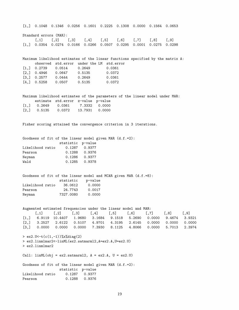
[1,] 0.1048 0.1346 0.0256 0.1601 0.2225 0.1308 0.0000 0.1564 0.0653
Standard errors (MAR):[,1] [,2] [,3] [,4] [,5] [,6] [,7] [,8] [,9]
[1,] 0.0354 0.0274 0.0166 0.0266 0.0507 0.0295 0.0001 0.0275 0.0298
Maximum likelihood estimates of the linear functions specified by the matrix A:observed std.error under the LM std.error
[1,] 0.2739 0.0514 0.2649 0.0361[2,] 0.4946 0.0647 0.5135 0.0372[3,] 0.2577 0.0444 0.2649 0.0361[4,] 0.5258 0.0507 0.5135 0.0372
Maximum likelihood estimates of the parameters of the linear model under MAR:estimate std.error z-value p-value
[1,] 0.2649 0.0361 7.3332 0.0000[2,] 0.5135 0.0372 13.7931 0.0000
Fisher scoring attained the convergence criterion in 3 iterations.
Goodness of fit of the linear model given MAR (d.f.=2):statistic p-value
Likelihood ratio 0.1287 0.9377Pearson 0.1288 0.9376Neyman 0.1286 0.9377Wald 0.1285 0.9378
Goodness of fit of the linear model and MCAR given MAR (d.f.=8):statistic p-value
Likelihood ratio 36.0612 0.0000Pearson 24.7743 0.0017Neyman 7327.0080 0.0000
Augmented estimated frequencies under the linear model and MAR:[,1] [,2] [,3] [,4] [,5] [,6] [,7] [,8] [,9]
[1,] 6.9119 10.4407 1.9680 3.1684 9.1518 5.2690 0.0000 9.4674 3.9321[2,] 3.2527 2.6122 0.5107 4.9701 4.3195 2.6145 0.0000 0.0000 0.0000[3,] 0.0000 0.0000 0.0000 7.3930 8.1125 4.8066 0.0000 5.7013 2.3974
> ex2.U<-t(c(1,-1))%x%diag(2)> ex2.linmlmar2<-linML(ex2.satmarml2,A=ex2.A,U=ex2.U)> ex2.linmlmar2
Call: linML(obj = ex2.satmarml2, A = ex2.A, U = ex2.U)
Goodness of fit of the linear model given MAR (d.f.=2):statistic p-value
Likelihood ratio 0.1287 0.9377Pearson 0.1288 0.9376
19
Neyman 0.1286 0.9377Wald 0.1285 0.9378
Goodness of fit of the linear model and MCAR given MAR (d.f.=8):statistic p-value
Likelihood ratio 36.0612 0.0000Pearson 24.7743 0.0017Neyman 7327.0080 0.0000
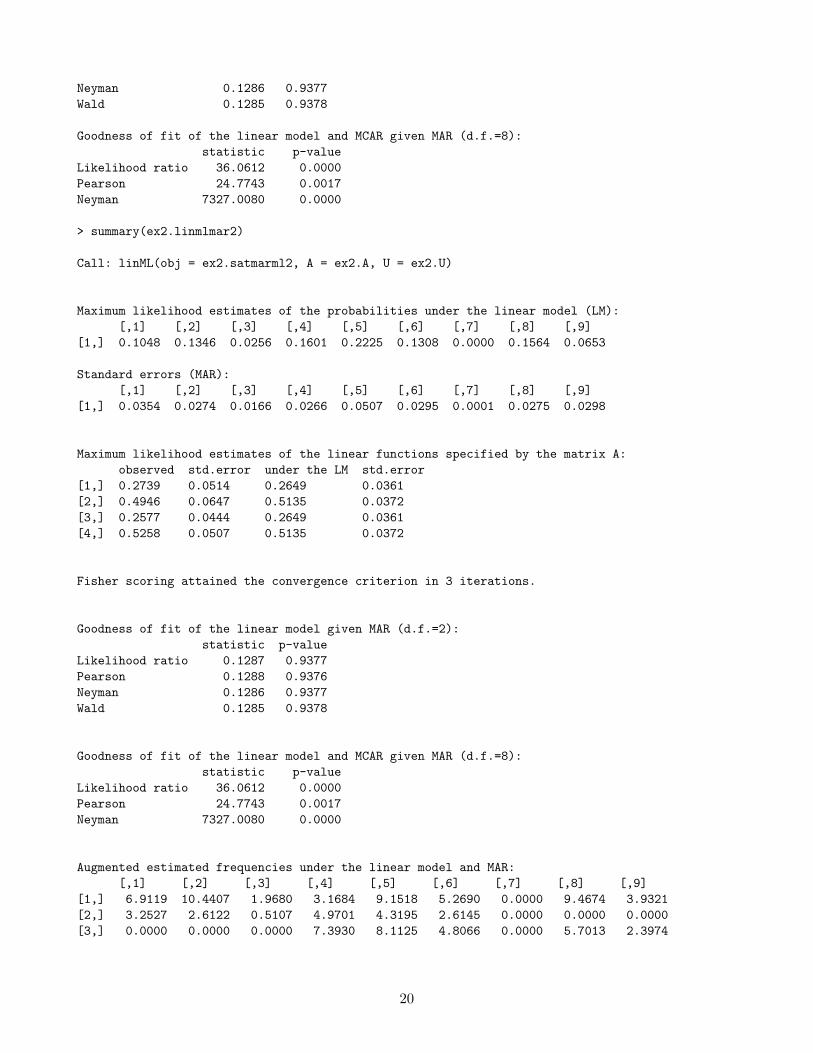
> summary(ex2.linmlmar2)
Call: linML(obj = ex2.satmarml2, A = ex2.A, U = ex2.U)
Maximum likelihood estimates of the probabilities under the linear model (LM):[,1] [,2] [,3] [,4] [,5] [,6] [,7] [,8] [,9]
[1,] 0.1048 0.1346 0.0256 0.1601 0.2225 0.1308 0.0000 0.1564 0.0653
Standard errors (MAR):[,1] [,2] [,3] [,4] [,5] [,6] [,7] [,8] [,9]
[1,] 0.0354 0.0274 0.0166 0.0266 0.0507 0.0295 0.0001 0.0275 0.0298
Maximum likelihood estimates of the linear functions specified by the matrix A:observed std.error under the LM std.error
[1,] 0.2739 0.0514 0.2649 0.0361[2,] 0.4946 0.0647 0.5135 0.0372[3,] 0.2577 0.0444 0.2649 0.0361[4,] 0.5258 0.0507 0.5135 0.0372
Fisher scoring attained the convergence criterion in 3 iterations.
Goodness of fit of the linear model given MAR (d.f.=2):statistic p-value
Likelihood ratio 0.1287 0.9377Pearson 0.1288 0.9376Neyman 0.1286 0.9377Wald 0.1285 0.9378
Goodness of fit of the linear model and MCAR given MAR (d.f.=8):statistic p-value
Likelihood ratio 36.0612 0.0000Pearson 24.7743 0.0017Neyman 7327.0080 0.0000
Augmented estimated frequencies under the linear model and MAR:[,1] [,2] [,3] [,4] [,5] [,6] [,7] [,8] [,9]
[1,] 6.9119 10.4407 1.9680 3.1684 9.1518 5.2690 0.0000 9.4674 3.9321[2,] 3.2527 2.6122 0.5107 4.9701 4.3195 2.6145 0.0000 0.0000 0.0000[3,] 0.0000 0.0000 0.0000 7.3930 8.1125 4.8066 0.0000 5.7013 2.3974
20
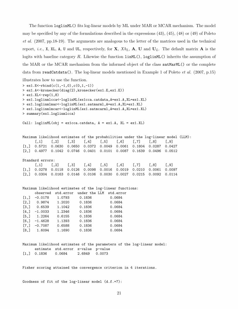
The function loglinML() fits log-linear models by ML under MAR or MCAR mechanism. The model
may be specified by any of the formulations described in the expressions (43), (45), (48) or (49) of Poleto
et al. (2007, pp.18-19). The arguments are analogous to the letter of the matrices used in the technical
report, i.e., X, XL, A, U and UL, respectively, for X, XbL, A, U and UL. The default matrix A is the
logits with baseline category R. Likewise the function linML(), loglinML() inherits the assumption of
the MAR or the MCAR mechanism from the informed object of the class satMarML() or the complete
data from readCatdata(). The log-linear models mentioned in Example 1 of Poleto et al. (2007, p.15)
illustrates how to use the function.> ex1.E<-rbind(c(1,-1,0),c(0,1,-1))> ex1.A<-kronecker(diag(2),kronecker(ex1.E,ex1.E))> ex1.XL<-rep(1,8)> ex1.loglinmlcca<-loglinML(ex1cca.catdata,A=ex1.A,XL=ex1.XL)> ex1.loglinmlmar<-loglinML(ex1.satmarml,A=ex1.A,XL=ex1.XL)> ex1.loglinmlmcar<-loglinML(ex1.satmcarml,A=ex1.A,XL=ex1.XL)> summary(ex1.loglinmlcca)
Call: loglinML(obj = ex1cca.catdata, A = ex1.A, XL = ex1.XL)
Maximum likelihood estimates of the probabilities under the log-linear model (LLM):[,1] [,2] [,3] [,4] [,5] [,6] [,7] [,8] [,9]
[1,] 0.5721 0.0630 0.0650 0.0372 0.0049 0.0061 0.1804 0.0287 0.0427[2,] 0.4977 0.1042 0.0746 0.0401 0.0101 0.0087 0.1639 0.0496 0.0512
Standard errors:[,1] [,2] [,3] [,4] [,5] [,6] [,7] [,8] [,9]
[1,] 0.0278 0.0118 0.0126 0.0098 0.0016 0.0019 0.0210 0.0061 0.0097[2,] 0.0304 0.0163 0.0146 0.0106 0.0030 0.0027 0.0215 0.0092 0.0114
Maximum likelihood estimates of the log-linear functions:observed std.error under the LLM std.error
[1,] -0.0178 1.0793 0.1836 0.0684[2,] 0.9874 1.2020 0.1836 0.0684[3,] 0.6539 1.1042 0.1836 0.0684[4,] -1.0033 1.2346 0.1836 0.0684[5,] 1.2264 0.6155 0.1836 0.0684[6,] -1.4628 1.1393 0.1836 0.0684[7,] -0.7087 0.6588 0.1836 0.0684[8,] 1.6094 1.1690 0.1836 0.0684
Maximum likelihood estimates of the parameters of the log-linear model:estimate std.error z-value p-value
[1,] 0.1836 0.0684 2.6849 0.0073
Fisher scoring attained the convergence criterion in 4 iterations.
Goodness of fit of the log-linear model (d.f.=7):
21
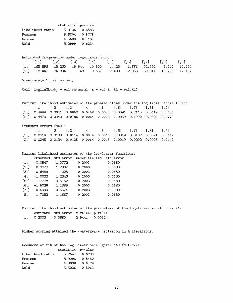
statistic p-valueLikelihood ratio 5.0136 0.6583Pearson 5.6804 0.5775Neyman 4.5583 0.7137Wald 5.2999 0.6234
Estimated frequencies under log-linear model:[,1] [,2] [,3] [,4] [,5] [,6] [,7] [,8] [,9]
[1,] 165.896 18.260 18.844 10.800 1.428 1.771 52.304 8.312 12.384[2,] 118.447 24.804 17.749 9.537 2.400 2.063 39.017 11.796 12.187
> summary(ex1.loglinmlmar)
Call: loglinML(obj = ex1.satmarml, A = ex1.A, XL = ex1.XL)
Maximum likelihood estimates of the probabilities under the log-linear model (LLM):[,1] [,2] [,3] [,4] [,5] [,6] [,7] [,8] [,9]
[1,] 0.4888 0.0641 0.0652 0.0458 0.0073 0.0091 0.2140 0.0419 0.0636[2,] 0.4479 0.0940 0.0786 0.0264 0.0068 0.0069 0.1992 0.0624 0.0778
Standard errors (MAR):[,1] [,2] [,3] [,4] [,5] [,6] [,7] [,8] [,9]
[1,] 0.0214 0.0103 0.0114 0.0074 0.0016 0.0019 0.0182 0.0071 0.0119[2,] 0.0245 0.0134 0.0135 0.0064 0.0018 0.0019 0.0202 0.0095 0.0140
Maximum likelihood estimates of the log-linear functions:observed std.error under the LLM std.error
[1,] 0.0547 1.0772 0.2003 0.0680[2,] 0.9878 1.2007 0.2003 0.0680[3,] 0.6489 1.1028 0.2003 0.0680[4,] -1.0033 1.2346 0.2003 0.0680[5,] 1.2228 0.6152 0.2003 0.0680[6,] -1.5026 1.1389 0.2003 0.0680[7,] -0.6999 0.6574 0.2003 0.0680[8,] 1.7083 1.1667 0.2003 0.0680
Maximum likelihood estimates of the parameters of the log-linear model under MAR:estimate std.error z-value p-value
[1,] 0.2003 0.0680 2.9441 0.0032
Fisher scoring attained the convergence criterion in 4 iterations.
Goodness of fit of the log-linear model given MAR (d.f.=7):statistic p-value
Likelihood ratio 5.2547 0.6289Pearson 5.9298 0.5480Neyman 4.8938 0.6729Wald 5.5236 0.5963
22
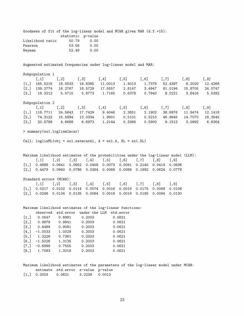
Goodness of fit of the log-linear model and MCAR given MAR (d.f.=15):statistic p-value
Likelihood ratio 50.79 0.00Pearson 53.56 0.00Neyman 52.49 0.00
Augmented estimated frequencies under log-linear model and MAR:
Subpopulation 1[,1] [,2] [,3] [,4] [,5] [,6] [,7] [,8] [,9]
[1,] 165.5216 18.5533 18.8385 11.0013 1.4013 1.7376 52.4397 8.2020 12.4268[2,] 139.2774 18.2767 18.5729 17.5557 2.8147 3.4947 81.0194 15.8705 24.0747[3,] 18.3212 5.5715 5.6773 1.7165 0.6378 0.7940 8.0221 3.6416 5.5392
Subpopulation 2[,1] [,2] [,3] [,4] [,5] [,6] [,7] [,8] [,9]
[1,] 118.7711 24.5643 17.7429 9.4046 2.3851 2.1902 38.8976 11.9474 12.1418[2,] 74.3122 15.5894 13.0334 1.9901 0.5101 0.5210 46.9645 14.7070 18.3545[3,] 20.5788 4.6688 6.6973 1.2144 0.3366 0.5900 9.1512 3.0992 6.6364
> summary(ex1.loglinmlmcar)
Call: loglinML(obj = ex1.satmcarml, A = ex1.A, XL = ex1.XL)
Maximum likelihood estimates of the probabilities under the log-linear model (LLM):[,1] [,2] [,3] [,4] [,5] [,6] [,7] [,8] [,9]
[1,] 0.4888 0.0641 0.0652 0.0458 0.0073 0.0091 0.2140 0.0419 0.0636[2,] 0.4479 0.0940 0.0786 0.0264 0.0068 0.0069 0.1992 0.0624 0.0778
Standard errors (MCAR):[,1] [,2] [,3] [,4] [,5] [,6] [,7] [,8] [,9]
[1,] 0.0217 0.0102 0.0114 0.0074 0.0016 0.0019 0.0175 0.0069 0.0108[2,] 0.0248 0.0134 0.0135 0.0064 0.0018 0.0019 0.0195 0.0094 0.0130
Maximum likelihood estimates of the log-linear functions:observed std.error under the LLM std.error
[1,] 0.0547 0.8981 0.2003 0.0621[2,] 0.9878 0.9941 0.2003 0.0621[3,] 0.6489 0.9081 0.2003 0.0621[4,] -1.0033 1.0029 0.2003 0.0621[5,] 1.2228 0.7361 0.2003 0.0621[6,] -1.5026 1.3135 0.2003 0.0621[7,] -0.6999 0.7555 0.2003 0.0621[8,] 1.7083 1.3218 0.2003 0.0621
Maximum likelihood estimates of the parameters of the log-linear model under MCAR:estimate std.error z-value p-value
[1,] 0.2003 0.0621 3.2239 0.0013
23
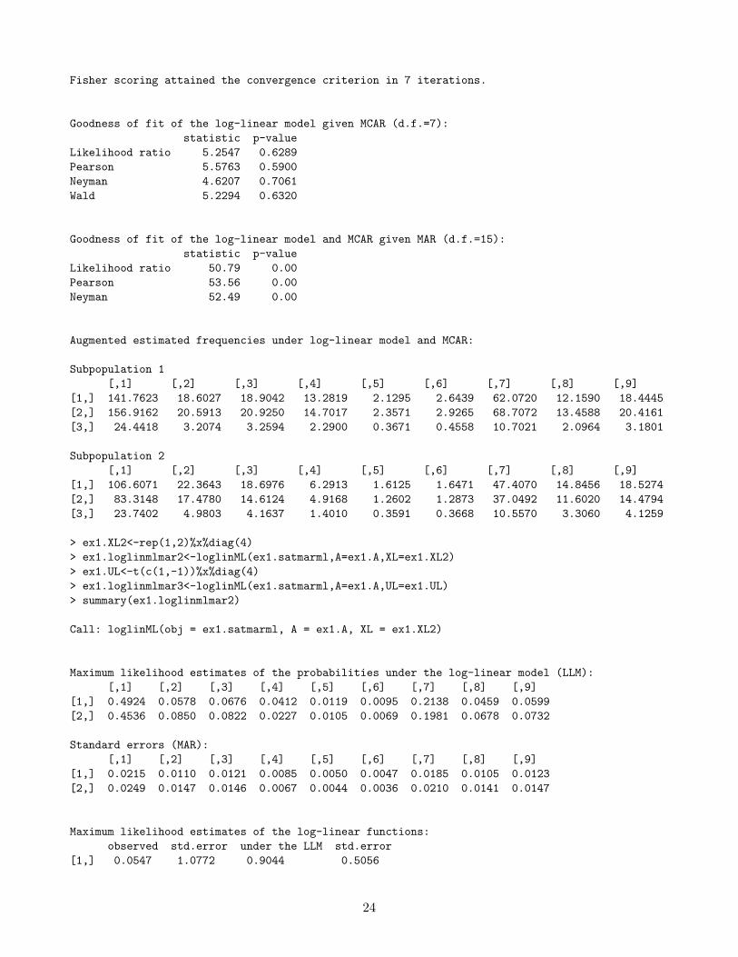
Fisher scoring attained the convergence criterion in 7 iterations.
Goodness of fit of the log-linear model given MCAR (d.f.=7):statistic p-value
Likelihood ratio 5.2547 0.6289Pearson 5.5763 0.5900Neyman 4.6207 0.7061Wald 5.2294 0.6320
Goodness of fit of the log-linear model and MCAR given MAR (d.f.=15):statistic p-value
Likelihood ratio 50.79 0.00Pearson 53.56 0.00Neyman 52.49 0.00
Augmented estimated frequencies under log-linear model and MCAR:
Subpopulation 1[,1] [,2] [,3] [,4] [,5] [,6] [,7] [,8] [,9]
[1,] 141.7623 18.6027 18.9042 13.2819 2.1295 2.6439 62.0720 12.1590 18.4445[2,] 156.9162 20.5913 20.9250 14.7017 2.3571 2.9265 68.7072 13.4588 20.4161[3,] 24.4418 3.2074 3.2594 2.2900 0.3671 0.4558 10.7021 2.0964 3.1801
Subpopulation 2[,1] [,2] [,3] [,4] [,5] [,6] [,7] [,8] [,9]
[1,] 106.6071 22.3643 18.6976 6.2913 1.6125 1.6471 47.4070 14.8456 18.5274[2,] 83.3148 17.4780 14.6124 4.9168 1.2602 1.2873 37.0492 11.6020 14.4794[3,] 23.7402 4.9803 4.1637 1.4010 0.3591 0.3668 10.5570 3.3060 4.1259
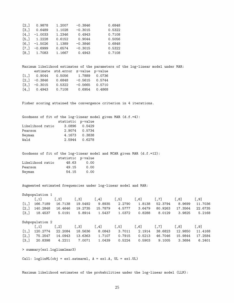
> ex1.XL2<-rep(1,2)%x%diag(4)> ex1.loglinmlmar2<-loglinML(ex1.satmarml,A=ex1.A,XL=ex1.XL2)> ex1.UL<-t(c(1,-1))%x%diag(4)> ex1.loglinmlmar3<-loglinML(ex1.satmarml,A=ex1.A,UL=ex1.UL)> summary(ex1.loglinmlmar2)
Call: loglinML(obj = ex1.satmarml, A = ex1.A, XL = ex1.XL2)
Maximum likelihood estimates of the probabilities under the log-linear model (LLM):[,1] [,2] [,3] [,4] [,5] [,6] [,7] [,8] [,9]
[1,] 0.4924 0.0578 0.0676 0.0412 0.0119 0.0095 0.2138 0.0459 0.0599[2,] 0.4536 0.0850 0.0822 0.0227 0.0105 0.0069 0.1981 0.0678 0.0732
Standard errors (MAR):[,1] [,2] [,3] [,4] [,5] [,6] [,7] [,8] [,9]
[1,] 0.0215 0.0110 0.0121 0.0085 0.0050 0.0047 0.0185 0.0105 0.0123[2,] 0.0249 0.0147 0.0146 0.0067 0.0044 0.0036 0.0210 0.0141 0.0147
Maximum likelihood estimates of the log-linear functions:observed std.error under the LLM std.error
[1,] 0.0547 1.0772 0.9044 0.5056
24
[2,] 0.9878 1.2007 -0.3846 0.6848[3,] 0.6489 1.1028 -0.3015 0.5322[4,] -1.0033 1.2346 0.4943 0.7108[5,] 1.2228 0.6152 0.9044 0.5056[6,] -1.5026 1.1389 -0.3846 0.6848[7,] -0.6999 0.6574 -0.3015 0.5322[8,] 1.7083 1.1667 0.4943 0.7108
Maximum likelihood estimates of the parameters of the log-linear model under MAR:estimate std.error z-value p-value
[1,] 0.9044 0.5056 1.7889 0.0736[2,] -0.3846 0.6848 -0.5615 0.5744[3,] -0.3015 0.5322 -0.5665 0.5710[4,] 0.4943 0.7108 0.6954 0.4868
Fisher scoring attained the convergence criterion in 4 iterations.
Goodness of fit of the log-linear model given MAR (d.f.=4):statistic p-value
Likelihood ratio 3.0896 0.5429Pearson 2.9074 0.5734Neyman 4.1673 0.3838Wald 2.5944 0.6278
Goodness of fit of the log-linear model and MCAR given MAR (d.f.=12):statistic p-value
Likelihood ratio 48.63 0.00Pearson 49.15 0.00Neyman 54.15 0.00
Augmented estimated frequencies under log-linear model and MAR:
Subpopulation 1[,1] [,2] [,3] [,4] [,5] [,6] [,7] [,8] [,9]
[1,] 166.7189 16.7138 19.5492 9.8935 2.2790 1.8138 52.3794 8.9699 11.7036[2,] 140.2848 16.4646 19.2735 15.7879 4.5777 3.6479 80.9263 17.3564 22.6735[3,] 18.4537 5.0191 5.8914 1.5437 1.0372 0.8288 8.0129 3.9825 5.2168
Subpopulation 2[,1] [,2] [,3] [,4] [,5] [,6] [,7] [,8] [,9]
[1,] 120.2774 22.2084 18.5636 8.0843 3.7011 2.1914 38.6823 12.9850 11.4168[2,] 75.2547 14.0943 13.6363 1.7107 0.7915 0.5213 46.7046 15.9844 17.2584[3,] 20.8398 4.2211 7.0071 1.0439 0.5224 0.5903 9.1005 3.3684 6.2401
> summary(ex1.loglinmlmar3)
Call: loglinML(obj = ex1.satmarml, A = ex1.A, UL = ex1.UL)
Maximum likelihood estimates of the probabilities under the log-linear model (LLM):
25
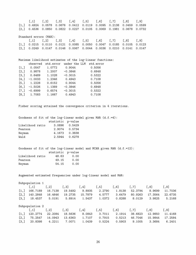
[,1] [,2] [,3] [,4] [,5] [,6] [,7] [,8] [,9][1,] 0.4924 0.0578 0.0676 0.0412 0.0119 0.0095 0.2138 0.0459 0.0599[2,] 0.4536 0.0850 0.0822 0.0227 0.0105 0.0069 0.1981 0.0678 0.0732
Standard errors (MAR):[,1] [,2] [,3] [,4] [,5] [,6] [,7] [,8] [,9]
[1,] 0.0215 0.0110 0.0121 0.0085 0.0050 0.0047 0.0185 0.0105 0.0123[2,] 0.0249 0.0147 0.0146 0.0067 0.0044 0.0036 0.0210 0.0141 0.0147
Maximum likelihood estimates of the log-linear functions:observed std.error under the LLM std.error
[1,] 0.0547 1.0772 0.9044 0.5056[2,] 0.9878 1.2007 -0.3846 0.6848[3,] 0.6489 1.1028 -0.3015 0.5322[4,] -1.0033 1.2346 0.4943 0.7108[5,] 1.2228 0.6152 0.9044 0.5056[6,] -1.5026 1.1389 -0.3846 0.6848[7,] -0.6999 0.6574 -0.3015 0.5322[8,] 1.7083 1.1667 0.4943 0.7108
Fisher scoring attained the convergence criterion in 4 iterations.
Goodness of fit of the log-linear model given MAR (d.f.=4):statistic p-value
Likelihood ratio 3.0896 0.5429Pearson 2.9074 0.5734Neyman 4.1673 0.3838Wald 2.5944 0.6278
Goodness of fit of the log-linear model and MCAR given MAR (d.f.=12):statistic p-value
Likelihood ratio 48.63 0.00Pearson 49.15 0.00Neyman 54.15 0.00
Augmented estimated frequencies under log-linear model and MAR:
Subpopulation 1[,1] [,2] [,3] [,4] [,5] [,6] [,7] [,8] [,9]
[1,] 166.7189 16.7138 19.5492 9.8935 2.2790 1.8138 52.3794 8.9699 11.7036[2,] 140.2848 16.4646 19.2735 15.7879 4.5777 3.6479 80.9263 17.3564 22.6735[3,] 18.4537 5.0191 5.8914 1.5437 1.0372 0.8288 8.0129 3.9825 5.2168
Subpopulation 2[,1] [,2] [,3] [,4] [,5] [,6] [,7] [,8] [,9]
[1,] 120.2774 22.2084 18.5636 8.0843 3.7011 2.1914 38.6823 12.9850 11.4168[2,] 75.2547 14.0943 13.6363 1.7107 0.7915 0.5213 46.7046 15.9844 17.2584[3,] 20.8398 4.2211 7.0071 1.0439 0.5224 0.5903 9.1005 3.3684 6.2401
26
Both linML() and loglinML() functions accept the arguments maxit, epsilon1 and epsilon2, as
described in Section 4.1
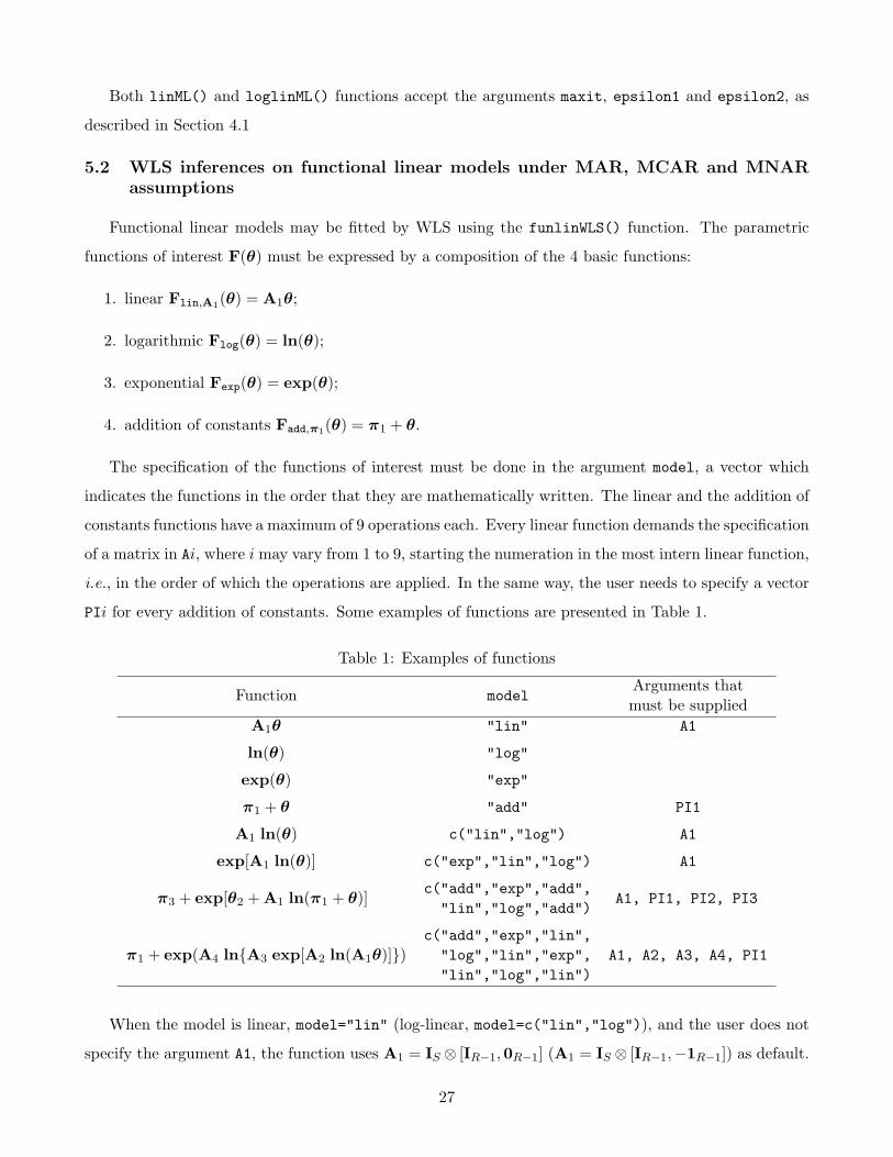
5.2 WLS inferences on functional linear models under MAR, MCAR and MNARassumptions
Functional linear models may be fitted by WLS using the funlinWLS() function. The parametric
functions of interest F(θ) must be expressed by a composition of the 4 basic functions:
1. linear Flin,A1(θ) = A1θ;
2. logarithmic Flog(θ) = ln(θ);
3. exponential Fexp(θ) = exp(θ);
4. addition of constants Fadd,π1(θ) = π1 + θ.
The specification of the functions of interest must be done in the argument model, a vector which
indicates the functions in the order that they are mathematically written. The linear and the addition of
constants functions have a maximum of 9 operations each. Every linear function demands the specification
of a matrix in Ai, where i may vary from 1 to 9, starting the numeration in the most intern linear function,
i.e., in the order of which the operations are applied. In the same way, the user needs to specify a vector
PIi for every addition of constants. Some examples of functions are presented in Table 1.
Table 1: Examples of functions
Function modelArguments thatmust be supplied
A1θ "lin" A1
ln(θ) "log"
exp(θ) "exp"
π1 + θ "add" PI1
A1 ln(θ) c("lin","log") A1
exp[A1 ln(θ)] c("exp","lin","log") A1
π3 + exp[θ2 + A1 ln(π1 + θ)]c("add","exp","add",
A1, PI1, PI2, PI3"lin","log","add")
c("add","exp","lin",π1 + exp(A4 ln{A3 exp[A2 ln(A1θ)]}) "log","lin","exp", A1, A2, A3, A4, PI1
"lin","log","lin")
When the model is linear, model="lin" (log-linear, model=c("lin","log")), and the user does not
specify the argument A1, the function uses A1 = IS ⊗ [IR−1,0R−1] (A1 = IS ⊗ [IR−1,−1R−1]) as default.
27
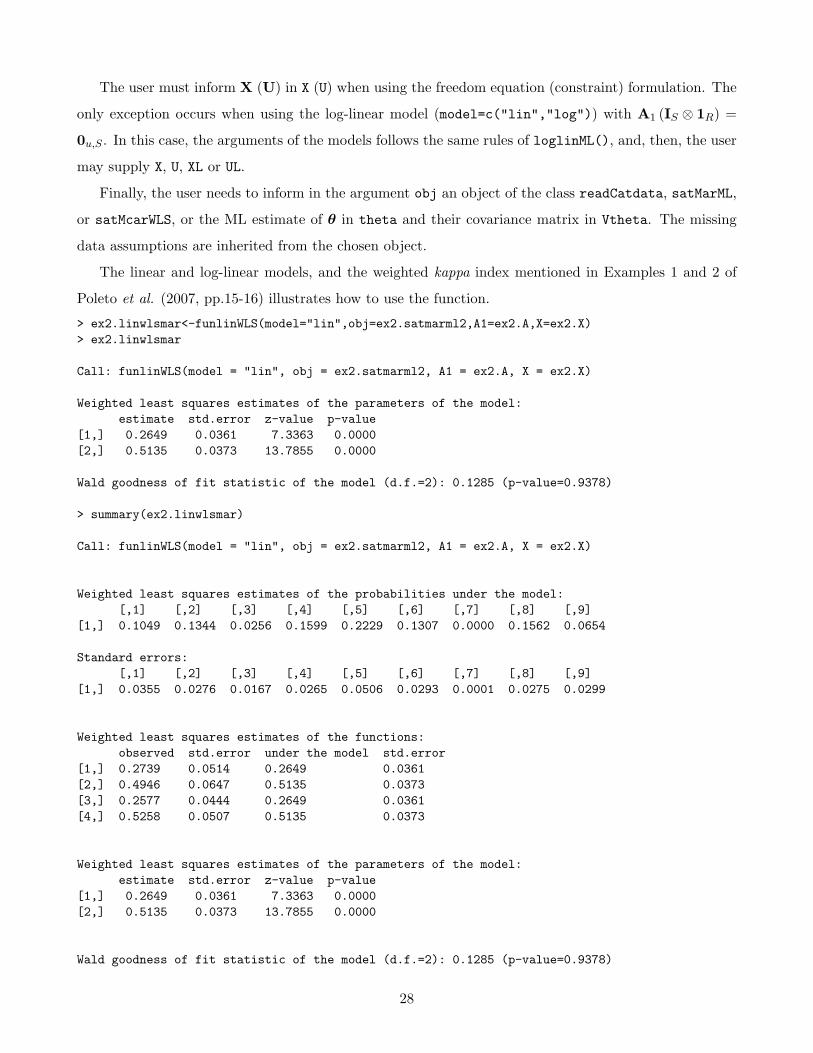
The user must inform X (U) in X (U) when using the freedom equation (constraint) formulation. The
only exception occurs when using the log-linear model (model=c("lin","log")) with A1 (IS ⊗ 1R) =
0u,S . In this case, the arguments of the models follows the same rules of loglinML(), and, then, the user
may supply X, U, XL or UL.
Finally, the user needs to inform in the argument obj an object of the class readCatdata, satMarML,
or satMcarWLS, or the ML estimate of θ in theta and their covariance matrix in Vtheta. The missing
data assumptions are inherited from the chosen object.
The linear and log-linear models, and the weighted kappa index mentioned in Examples 1 and 2 of
Poleto et al. (2007, pp.15-16) illustrates how to use the function.
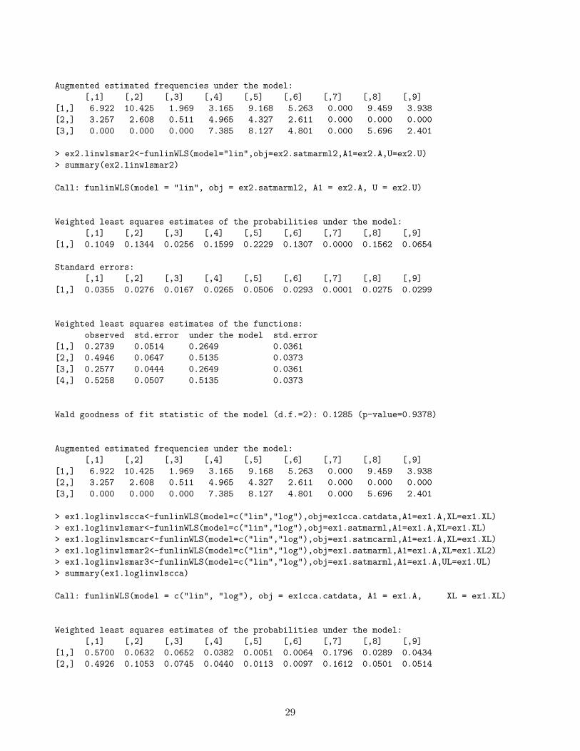
> ex2.linwlsmar<-funlinWLS(model="lin",obj=ex2.satmarml2,A1=ex2.A,X=ex2.X)> ex2.linwlsmar
Call: funlinWLS(model = "lin", obj = ex2.satmarml2, A1 = ex2.A, X = ex2.X)
Weighted least squares estimates of the parameters of the model:estimate std.error z-value p-value
[1,] 0.2649 0.0361 7.3363 0.0000[2,] 0.5135 0.0373 13.7855 0.0000
Wald goodness of fit statistic of the model (d.f.=2): 0.1285 (p-value=0.9378)
> summary(ex2.linwlsmar)
Call: funlinWLS(model = "lin", obj = ex2.satmarml2, A1 = ex2.A, X = ex2.X)
Weighted least squares estimates of the probabilities under the model:[,1] [,2] [,3] [,4] [,5] [,6] [,7] [,8] [,9]
[1,] 0.1049 0.1344 0.0256 0.1599 0.2229 0.1307 0.0000 0.1562 0.0654
Standard errors:[,1] [,2] [,3] [,4] [,5] [,6] [,7] [,8] [,9]
[1,] 0.0355 0.0276 0.0167 0.0265 0.0506 0.0293 0.0001 0.0275 0.0299
Weighted least squares estimates of the functions:observed std.error under the model std.error
[1,] 0.2739 0.0514 0.2649 0.0361[2,] 0.4946 0.0647 0.5135 0.0373[3,] 0.2577 0.0444 0.2649 0.0361[4,] 0.5258 0.0507 0.5135 0.0373
Weighted least squares estimates of the parameters of the model:estimate std.error z-value p-value
[1,] 0.2649 0.0361 7.3363 0.0000[2,] 0.5135 0.0373 13.7855 0.0000
Wald goodness of fit statistic of the model (d.f.=2): 0.1285 (p-value=0.9378)
28
Augmented estimated frequencies under the model:[,1] [,2] [,3] [,4] [,5] [,6] [,7] [,8] [,9]
[1,] 6.922 10.425 1.969 3.165 9.168 5.263 0.000 9.459 3.938[2,] 3.257 2.608 0.511 4.965 4.327 2.611 0.000 0.000 0.000[3,] 0.000 0.000 0.000 7.385 8.127 4.801 0.000 5.696 2.401
> ex2.linwlsmar2<-funlinWLS(model="lin",obj=ex2.satmarml2,A1=ex2.A,U=ex2.U)> summary(ex2.linwlsmar2)
Call: funlinWLS(model = "lin", obj = ex2.satmarml2, A1 = ex2.A, U = ex2.U)
Weighted least squares estimates of the probabilities under the model:[,1] [,2] [,3] [,4] [,5] [,6] [,7] [,8] [,9]
[1,] 0.1049 0.1344 0.0256 0.1599 0.2229 0.1307 0.0000 0.1562 0.0654
Standard errors:[,1] [,2] [,3] [,4] [,5] [,6] [,7] [,8] [,9]
[1,] 0.0355 0.0276 0.0167 0.0265 0.0506 0.0293 0.0001 0.0275 0.0299
Weighted least squares estimates of the functions:observed std.error under the model std.error
[1,] 0.2739 0.0514 0.2649 0.0361[2,] 0.4946 0.0647 0.5135 0.0373[3,] 0.2577 0.0444 0.2649 0.0361[4,] 0.5258 0.0507 0.5135 0.0373
Wald goodness of fit statistic of the model (d.f.=2): 0.1285 (p-value=0.9378)
Augmented estimated frequencies under the model:[,1] [,2] [,3] [,4] [,5] [,6] [,7] [,8] [,9]
[1,] 6.922 10.425 1.969 3.165 9.168 5.263 0.000 9.459 3.938[2,] 3.257 2.608 0.511 4.965 4.327 2.611 0.000 0.000 0.000[3,] 0.000 0.000 0.000 7.385 8.127 4.801 0.000 5.696 2.401
> ex1.loglinwlscca<-funlinWLS(model=c("lin","log"),obj=ex1cca.catdata,A1=ex1.A,XL=ex1.XL)> ex1.loglinwlsmar<-funlinWLS(model=c("lin","log"),obj=ex1.satmarml,A1=ex1.A,XL=ex1.XL)> ex1.loglinwlsmcar<-funlinWLS(model=c("lin","log"),obj=ex1.satmcarml,A1=ex1.A,XL=ex1.XL)> ex1.loglinwlsmar2<-funlinWLS(model=c("lin","log"),obj=ex1.satmarml,A1=ex1.A,XL=ex1.XL2)> ex1.loglinwlsmar3<-funlinWLS(model=c("lin","log"),obj=ex1.satmarml,A1=ex1.A,UL=ex1.UL)> summary(ex1.loglinwlscca)
Call: funlinWLS(model = c("lin", "log"), obj = ex1cca.catdata, A1 = ex1.A, XL = ex1.XL)
Weighted least squares estimates of the probabilities under the model:[,1] [,2] [,3] [,4] [,5] [,6] [,7] [,8] [,9]
[1,] 0.5700 0.0632 0.0652 0.0382 0.0051 0.0064 0.1796 0.0289 0.0434[2,] 0.4926 0.1053 0.0745 0.0440 0.0113 0.0097 0.1612 0.0501 0.0514
29
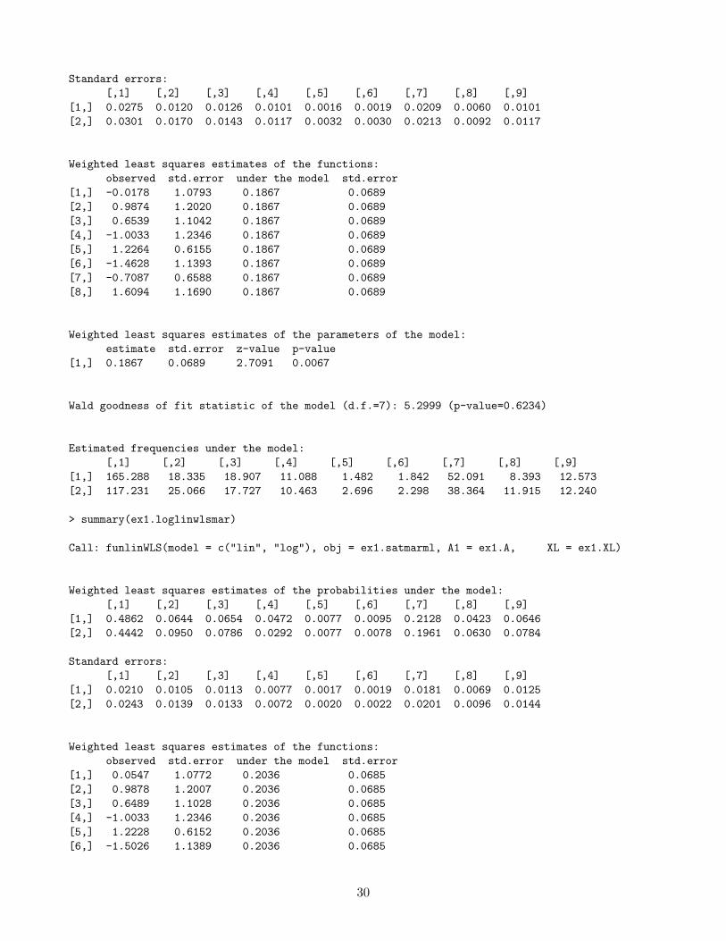
Standard errors:[,1] [,2] [,3] [,4] [,5] [,6] [,7] [,8] [,9]
[1,] 0.0275 0.0120 0.0126 0.0101 0.0016 0.0019 0.0209 0.0060 0.0101[2,] 0.0301 0.0170 0.0143 0.0117 0.0032 0.0030 0.0213 0.0092 0.0117
Weighted least squares estimates of the functions:observed std.error under the model std.error
[1,] -0.0178 1.0793 0.1867 0.0689[2,] 0.9874 1.2020 0.1867 0.0689[3,] 0.6539 1.1042 0.1867 0.0689[4,] -1.0033 1.2346 0.1867 0.0689[5,] 1.2264 0.6155 0.1867 0.0689[6,] -1.4628 1.1393 0.1867 0.0689[7,] -0.7087 0.6588 0.1867 0.0689[8,] 1.6094 1.1690 0.1867 0.0689
Weighted least squares estimates of the parameters of the model:estimate std.error z-value p-value
[1,] 0.1867 0.0689 2.7091 0.0067
Wald goodness of fit statistic of the model (d.f.=7): 5.2999 (p-value=0.6234)
Estimated frequencies under the model:[,1] [,2] [,3] [,4] [,5] [,6] [,7] [,8] [,9]
[1,] 165.288 18.335 18.907 11.088 1.482 1.842 52.091 8.393 12.573[2,] 117.231 25.066 17.727 10.463 2.696 2.298 38.364 11.915 12.240
> summary(ex1.loglinwlsmar)
Call: funlinWLS(model = c("lin", "log"), obj = ex1.satmarml, A1 = ex1.A, XL = ex1.XL)
Weighted least squares estimates of the probabilities under the model:[,1] [,2] [,3] [,4] [,5] [,6] [,7] [,8] [,9]
[1,] 0.4862 0.0644 0.0654 0.0472 0.0077 0.0095 0.2128 0.0423 0.0646[2,] 0.4442 0.0950 0.0786 0.0292 0.0077 0.0078 0.1961 0.0630 0.0784
Standard errors:[,1] [,2] [,3] [,4] [,5] [,6] [,7] [,8] [,9]
[1,] 0.0210 0.0105 0.0113 0.0077 0.0017 0.0019 0.0181 0.0069 0.0125[2,] 0.0243 0.0139 0.0133 0.0072 0.0020 0.0022 0.0201 0.0096 0.0144
Weighted least squares estimates of the functions:observed std.error under the model std.error
[1,] 0.0547 1.0772 0.2036 0.0685[2,] 0.9878 1.2007 0.2036 0.0685[3,] 0.6489 1.1028 0.2036 0.0685[4,] -1.0033 1.2346 0.2036 0.0685[5,] 1.2228 0.6152 0.2036 0.0685[6,] -1.5026 1.1389 0.2036 0.0685
30

[7,] -0.6999 0.6574 0.2036 0.0685[8,] 1.7083 1.1667 0.2036 0.0685
Weighted least squares estimates of the parameters of the model:estimate std.error z-value p-value
[1,] 0.2036 0.0685 2.9709 0.0030
Wald goodness of fit statistic of the model (d.f.=7): 5.5236 (p-value=0.5963)
Augmented estimated frequencies under the model:
Subpopulation 1[,1] [,2] [,3] [,4] [,5] [,6] [,7] [,8] [,9]
[1,] 164.6298 18.6214 18.8879 11.3292 1.4610 1.8158 52.1307 8.2828 12.6198[2,] 138.5269 18.3437 18.6216 18.0789 2.9347 3.6520 80.5420 16.0269 24.4484[3,] 18.2225 5.5919 5.6922 1.7677 0.6650 0.8298 7.9748 3.6775 5.6252
Subpopulation 2[,1] [,2] [,3] [,4] [,5] [,6] [,7] [,8] [,9]
[1,] 117.7836 24.8266 17.7620 10.3893 2.6942 2.4587 38.3002 12.0691 12.2301[2,] 73.6944 15.7559 13.0475 2.1984 0.5762 0.5849 46.2432 14.8569 18.4879[3,] 20.4077 4.7187 6.7045 1.3416 0.3803 0.6623 9.0106 3.1308 6.6846
> summary(ex1.loglinwlsmcar)
Call: funlinWLS(model = c("lin", "log"), obj = ex1.satmcarml, A1 = ex1.A, XL = ex1.XL)
Weighted least squares estimates of the probabilities under the model:[,1] [,2] [,3] [,4] [,5] [,6] [,7] [,8] [,9]
[1,] 0.4842 0.0656 0.0658 0.0474 0.0078 0.0096 0.2128 0.0428 0.0639[2,] 0.4449 0.0936 0.0794 0.0293 0.0075 0.0078 0.1976 0.0618 0.0780
Standard errors:[,1] [,2] [,3] [,4] [,5] [,6] [,7] [,8] [,9]
[1,] 0.0213 0.0106 0.0114 0.0077 0.0017 0.0019 0.0175 0.0068 0.0113[2,] 0.0245 0.0138 0.0134 0.0072 0.0019 0.0022 0.0195 0.0093 0.0132
Weighted least squares estimates of the functions:observed std.error under the model std.error
[1,] 0.0547 0.8981 0.1983 0.0624[2,] 0.9878 0.9941 0.1983 0.0624[3,] 0.6489 0.9081 0.1983 0.0624[4,] -1.0033 1.0029 0.1983 0.0624[5,] 1.2228 0.7361 0.1983 0.0624[6,] -1.5026 1.3135 0.1983 0.0624[7,] -0.6999 0.7555 0.1983 0.0624[8,] 1.7083 1.3218 0.1983 0.0624
Weighted least squares estimates of the parameters of the model:
31
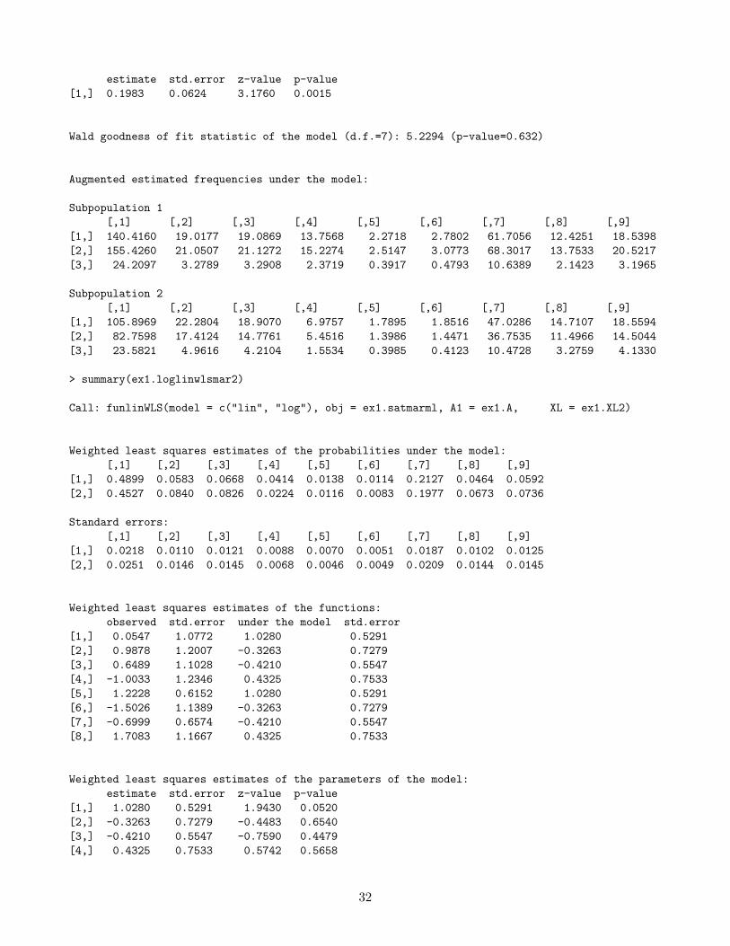
estimate std.error z-value p-value[1,] 0.1983 0.0624 3.1760 0.0015
Wald goodness of fit statistic of the model (d.f.=7): 5.2294 (p-value=0.632)
Augmented estimated frequencies under the model:
Subpopulation 1[,1] [,2] [,3] [,4] [,5] [,6] [,7] [,8] [,9]
[1,] 140.4160 19.0177 19.0869 13.7568 2.2718 2.7802 61.7056 12.4251 18.5398[2,] 155.4260 21.0507 21.1272 15.2274 2.5147 3.0773 68.3017 13.7533 20.5217[3,] 24.2097 3.2789 3.2908 2.3719 0.3917 0.4793 10.6389 2.1423 3.1965
Subpopulation 2[,1] [,2] [,3] [,4] [,5] [,6] [,7] [,8] [,9]
[1,] 105.8969 22.2804 18.9070 6.9757 1.7895 1.8516 47.0286 14.7107 18.5594[2,] 82.7598 17.4124 14.7761 5.4516 1.3986 1.4471 36.7535 11.4966 14.5044[3,] 23.5821 4.9616 4.2104 1.5534 0.3985 0.4123 10.4728 3.2759 4.1330
> summary(ex1.loglinwlsmar2)
Call: funlinWLS(model = c("lin", "log"), obj = ex1.satmarml, A1 = ex1.A, XL = ex1.XL2)
Weighted least squares estimates of the probabilities under the model:[,1] [,2] [,3] [,4] [,5] [,6] [,7] [,8] [,9]
[1,] 0.4899 0.0583 0.0668 0.0414 0.0138 0.0114 0.2127 0.0464 0.0592[2,] 0.4527 0.0840 0.0826 0.0224 0.0116 0.0083 0.1977 0.0673 0.0736
Standard errors:[,1] [,2] [,3] [,4] [,5] [,6] [,7] [,8] [,9]
[1,] 0.0218 0.0110 0.0121 0.0088 0.0070 0.0051 0.0187 0.0102 0.0125[2,] 0.0251 0.0146 0.0145 0.0068 0.0046 0.0049 0.0209 0.0144 0.0145
Weighted least squares estimates of the functions:observed std.error under the model std.error
[1,] 0.0547 1.0772 1.0280 0.5291[2,] 0.9878 1.2007 -0.3263 0.7279[3,] 0.6489 1.1028 -0.4210 0.5547[4,] -1.0033 1.2346 0.4325 0.7533[5,] 1.2228 0.6152 1.0280 0.5291[6,] -1.5026 1.1389 -0.3263 0.7279[7,] -0.6999 0.6574 -0.4210 0.5547[8,] 1.7083 1.1667 0.4325 0.7533
Weighted least squares estimates of the parameters of the model:estimate std.error z-value p-value
[1,] 1.0280 0.5291 1.9430 0.0520[2,] -0.3263 0.7279 -0.4483 0.6540[3,] -0.4210 0.5547 -0.7590 0.4479[4,] 0.4325 0.7533 0.5742 0.5658
32
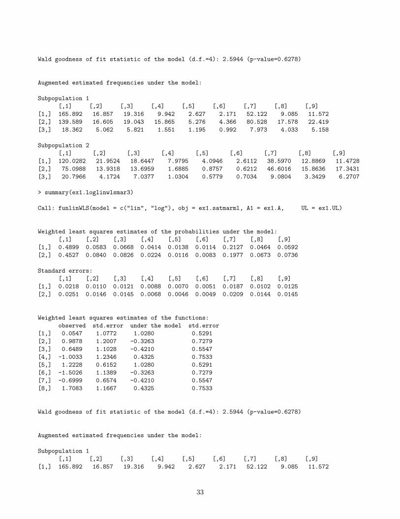
Wald goodness of fit statistic of the model (d.f.=4): 2.5944 (p-value=0.6278)
Augmented estimated frequencies under the model:
Subpopulation 1[,1] [,2] [,3] [,4] [,5] [,6] [,7] [,8] [,9]
[1,] 165.892 16.857 19.316 9.942 2.627 2.171 52.122 9.085 11.572[2,] 139.589 16.605 19.043 15.865 5.276 4.366 80.528 17.578 22.419[3,] 18.362 5.062 5.821 1.551 1.195 0.992 7.973 4.033 5.158
Subpopulation 2[,1] [,2] [,3] [,4] [,5] [,6] [,7] [,8] [,9]
[1,] 120.0282 21.9524 18.6447 7.9795 4.0946 2.6112 38.5970 12.8869 11.4728[2,] 75.0988 13.9318 13.6959 1.6885 0.8757 0.6212 46.6016 15.8636 17.3431[3,] 20.7966 4.1724 7.0377 1.0304 0.5779 0.7034 9.0804 3.3429 6.2707
> summary(ex1.loglinwlsmar3)
Call: funlinWLS(model = c("lin", "log"), obj = ex1.satmarml, A1 = ex1.A, UL = ex1.UL)
Weighted least squares estimates of the probabilities under the model:[,1] [,2] [,3] [,4] [,5] [,6] [,7] [,8] [,9]
[1,] 0.4899 0.0583 0.0668 0.0414 0.0138 0.0114 0.2127 0.0464 0.0592[2,] 0.4527 0.0840 0.0826 0.0224 0.0116 0.0083 0.1977 0.0673 0.0736
Standard errors:[,1] [,2] [,3] [,4] [,5] [,6] [,7] [,8] [,9]
[1,] 0.0218 0.0110 0.0121 0.0088 0.0070 0.0051 0.0187 0.0102 0.0125[2,] 0.0251 0.0146 0.0145 0.0068 0.0046 0.0049 0.0209 0.0144 0.0145
Weighted least squares estimates of the functions:observed std.error under the model std.error
[1,] 0.0547 1.0772 1.0280 0.5291[2,] 0.9878 1.2007 -0.3263 0.7279[3,] 0.6489 1.1028 -0.4210 0.5547[4,] -1.0033 1.2346 0.4325 0.7533[5,] 1.2228 0.6152 1.0280 0.5291[6,] -1.5026 1.1389 -0.3263 0.7279[7,] -0.6999 0.6574 -0.4210 0.5547[8,] 1.7083 1.1667 0.4325 0.7533
Wald goodness of fit statistic of the model (d.f.=4): 2.5944 (p-value=0.6278)
Augmented estimated frequencies under the model:
Subpopulation 1[,1] [,2] [,3] [,4] [,5] [,6] [,7] [,8] [,9]
[1,] 165.892 16.857 19.316 9.942 2.627 2.171 52.122 9.085 11.572
33
[2,] 139.589 16.605 19.043 15.865 5.276 4.366 80.528 17.578 22.419[3,] 18.362 5.062 5.821 1.551 1.195 0.992 7.973 4.033 5.158
Subpopulation 2[,1] [,2] [,3] [,4] [,5] [,6] [,7] [,8] [,9]
[1,] 120.0282 21.9524 18.6447 7.9795 4.0946 2.6112 38.5970 12.8869 11.4728[2,] 75.0988 13.9318 13.6959 1.6885 0.8757 0.6212 46.6016 15.8636 17.3431[3,] 20.7966 4.1724 7.0377 1.0304 0.5779 0.7034 9.0804 3.3429 6.2707
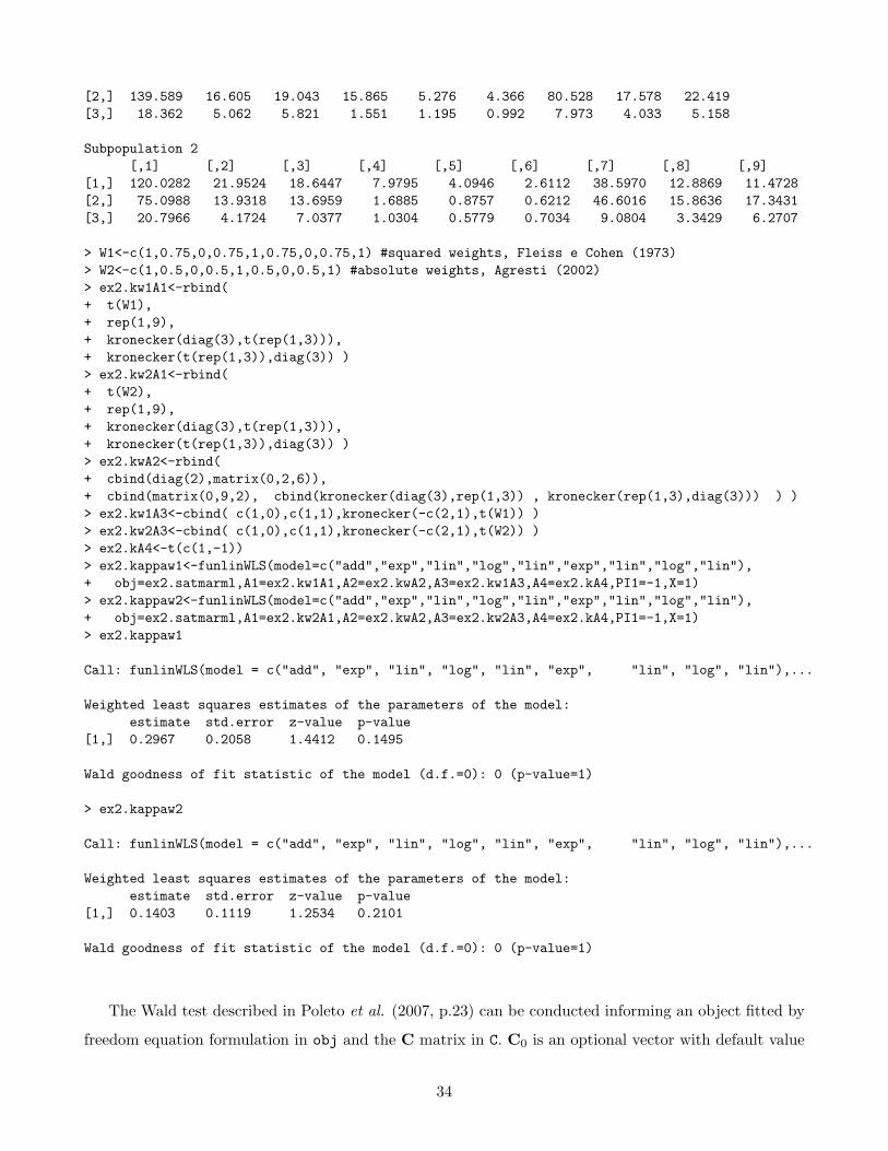
> W1<-c(1,0.75,0,0.75,1,0.75,0,0.75,1) #squared weights, Fleiss e Cohen (1973)> W2<-c(1,0.5,0,0.5,1,0.5,0,0.5,1) #absolute weights, Agresti (2002)> ex2.kw1A1<-rbind(+ t(W1),+ rep(1,9),+ kronecker(diag(3),t(rep(1,3))),+ kronecker(t(rep(1,3)),diag(3)) )> ex2.kw2A1<-rbind(+ t(W2),+ rep(1,9),+ kronecker(diag(3),t(rep(1,3))),+ kronecker(t(rep(1,3)),diag(3)) )> ex2.kwA2<-rbind(+ cbind(diag(2),matrix(0,2,6)),+ cbind(matrix(0,9,2), cbind(kronecker(diag(3),rep(1,3)) , kronecker(rep(1,3),diag(3))) ) )> ex2.kw1A3<-cbind( c(1,0),c(1,1),kronecker(-c(2,1),t(W1)) )> ex2.kw2A3<-cbind( c(1,0),c(1,1),kronecker(-c(2,1),t(W2)) )> ex2.kA4<-t(c(1,-1))> ex2.kappaw1<-funlinWLS(model=c("add","exp","lin","log","lin","exp","lin","log","lin"),+ obj=ex2.satmarml,A1=ex2.kw1A1,A2=ex2.kwA2,A3=ex2.kw1A3,A4=ex2.kA4,PI1=-1,X=1)> ex2.kappaw2<-funlinWLS(model=c("add","exp","lin","log","lin","exp","lin","log","lin"),+ obj=ex2.satmarml,A1=ex2.kw2A1,A2=ex2.kwA2,A3=ex2.kw2A3,A4=ex2.kA4,PI1=-1,X=1)> ex2.kappaw1
Call: funlinWLS(model = c("add", "exp", "lin", "log", "lin", "exp", "lin", "log", "lin"),...
Weighted least squares estimates of the parameters of the model:estimate std.error z-value p-value
[1,] 0.2967 0.2058 1.4412 0.1495
Wald goodness of fit statistic of the model (d.f.=0): 0 (p-value=1)
> ex2.kappaw2
Call: funlinWLS(model = c("add", "exp", "lin", "log", "lin", "exp", "lin", "log", "lin"),...
Weighted least squares estimates of the parameters of the model:estimate std.error z-value p-value
[1,] 0.1403 0.1119 1.2534 0.2101
Wald goodness of fit statistic of the model (d.f.=0): 0 (p-value=1)
The Wald test described in Poleto et al. (2007, p.23) can be conducted informing an object fitted by
freedom equation formulation in obj and the C matrix in C. C0 is an optional vector with default value
34
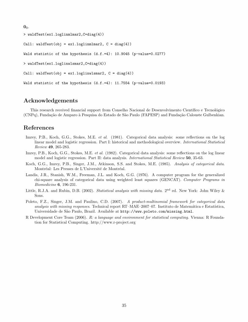
00.
> waldTest(ex1.loglinmlmar2,C=diag(4))
Call: waldTest(obj = ex1.loglinmlmar2, C = diag(4))
Wald statistic of the hypothesis (d.f.=4): 10.9045 (p-value=0.0277)
> waldTest(ex1.loglinwlsmar2,C=diag(4))
Call: waldTest(obj = ex1.loglinwlsmar2, C = diag(4))
Wald statistic of the hypothesis (d.f.=4): 11.7554 (p-value=0.0193)
Acknowledgements
This research received financial support from Conselho Nacional de Desenvolvimento Cientıfico e Tecnologico(CNPq), Fundacao de Amparo a Pesquisa do Estado de Sao Paulo (FAPESP) and Fundacao Calouste Gulbenkian.
References
Imrey, P.B., Koch, G.G., Stokes, M.E. et al. (1981). Categorical data analysis: some reflections on the loglinear model and logistic regression. Part I: historical and methodological overview. International StatisticalReview 49, 265-283.
Imrey, P.B., Koch, G.G., Stokes, M.E. et al. (1982). Categorical data analysis: some reflections on the log linearmodel and logistic regression. Part II: data analysis. International Statistical Review 50, 35-63.
Koch, G.G., Imrey, P.B., Singer, J.M., Atkinson, S.S. and Stokes, M.E. (1985). Analysis of categorical data.Montreal: Les Presses de L’Universite de Montreal.
Landis, J.R., Stanish, W.M., Freeman, J.L. and Koch, G.G. (1976). A computer program for the generalizedchi-square analysis of categorical data using weighted least squares (GENCAT). Computer Programs inBiomedicine 6, 196-231.
Little, R.J.A. and Rubin, D.B. (2002). Statistical analysis with missing data. 2nd ed. New York: John Wiley &Sons.
Poleto, F.Z., Singer, J.M. and Paulino, C.D. (2007). A product-multinomial framework for categorical dataanalysis with missing responses. Technical report RT–MAE–2007–07. Instituto de Matematica e Estatıstica,Universidade de Sao Paulo, Brazil. Available at http://www.poleto.com/missing.html.
R Development Core Team (2006). R: a language and environment for statistical computing. Vienna: R Founda-tion for Statistical Computing. http://www.r-project.org
35
Recommended