Application to transport phenomena
Current through an atomic metallic contact Shot noise in an atomic contact Current through a resonant level Current through a finite 1D region Multi-channel generalization: Concept of conduction eigenchannel
Current through an atomic metallic contact
STM fabricated MCBJ technique
AI
V
d.c. current through the contact
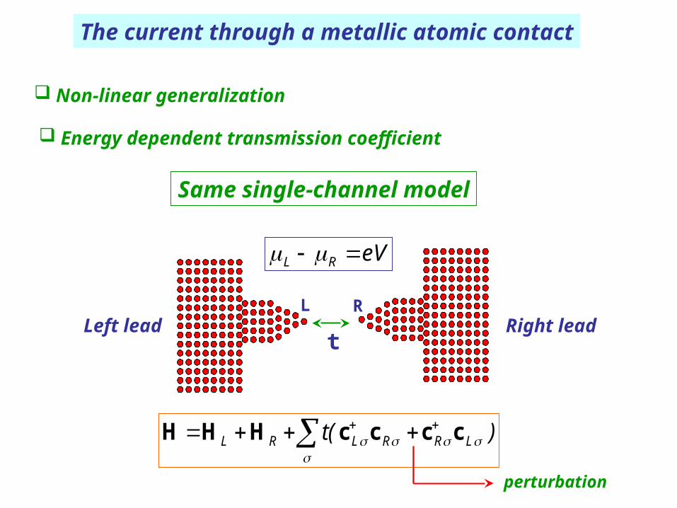
The current through a metallic atomic contact
Non-linear generalization
Energy dependent transmission coefficient
Same single-channel model
L R
tLeft lead Right lead
eVRL
)(t LRRLRL
ccccHHH perturbation
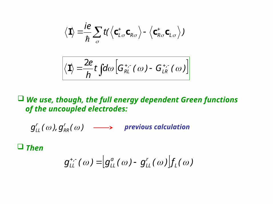
)(G)(Gdth
e ,LR
,RL
2I
)(tie
LRRL
ccccI
We use, though, the full energy dependent Green functions of the uncoupled electrodes:
)(g),(g rRR
rLL previous calculation
Then
)(f)(g)(g)(g LrLL
aLL
,LL
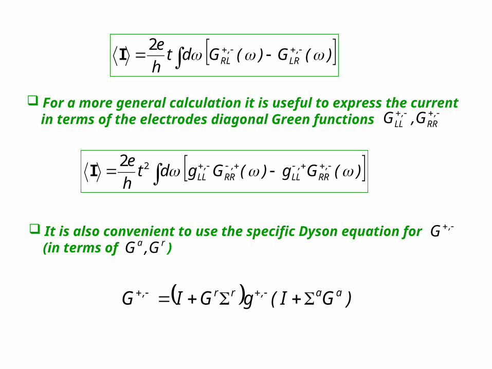
)(G)(Gdth
e ,LR
,RL
2I
For a more general calculation it is useful to express the current in terms of the electrodes diagonal Green functions
,RR
,LL G,G
It is also convenient to use the specific Dyson equation for (in terms of )
,Gra G,G
)(Gg)(Ggdth
e ,RR
,LL
,RR
,LL 2
2I
)GI(gGIG aa,rr,
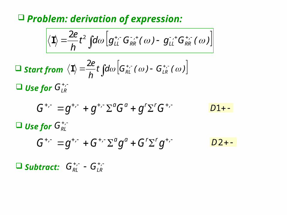
Problem: derivation of expression:
)(Gg)(Ggdth
e ,RR
,LL
,RR
,LL 2
2I
Start from )(G)(Gdth
e ,LR
,RL
2I
Use for ,
LRG
,rraa,,, GgGggG 1D
Use for ,
RLG
,rraa,,, gGgGgG 2D
Subtract: ,
LR,
RL GG
)(Gg)(Ggdth
e ,RR
,LL
,RR
,LL 2
2I
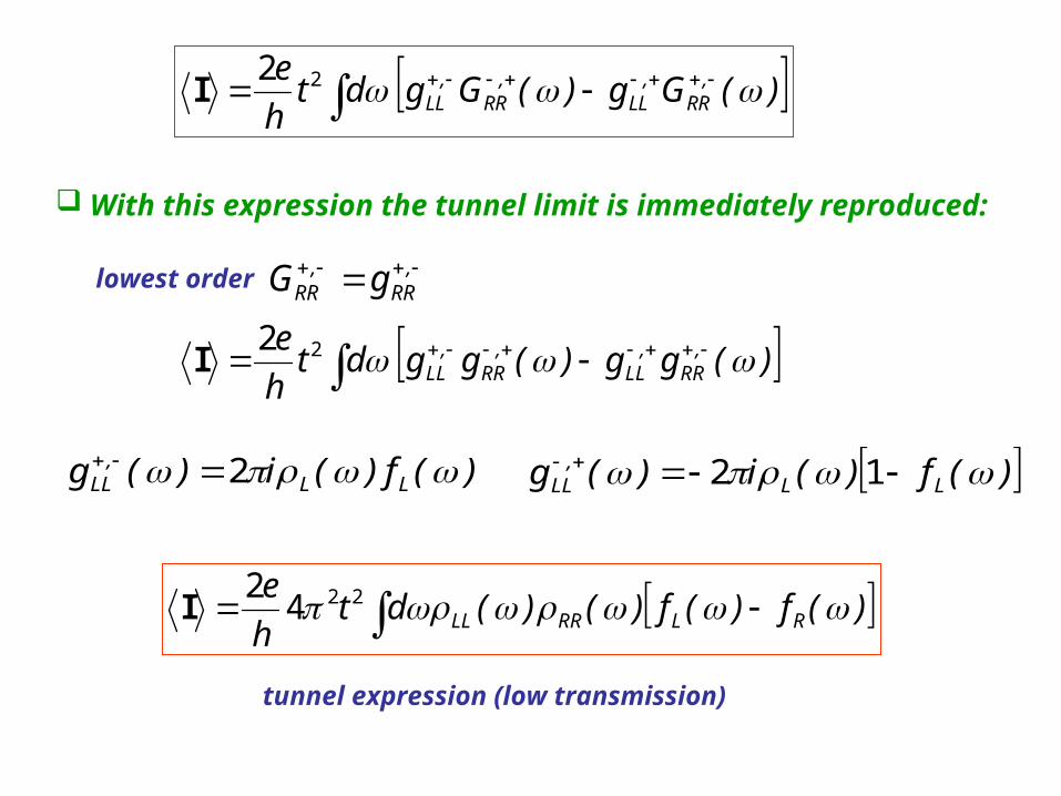
With this expression the tunnel limit is immediately reproduced:
lowest order ,RR
,RR gG
)(gg)(ggdth
e ,RR
,LL
,RR
,LL 2
2I
)(f)(i)(g LL,LL 2 )(f)(i)(g LL
,LL 12
)(f)(f)()(dth
eRLRRLL 224
2I
tunnel expression (low transmission)
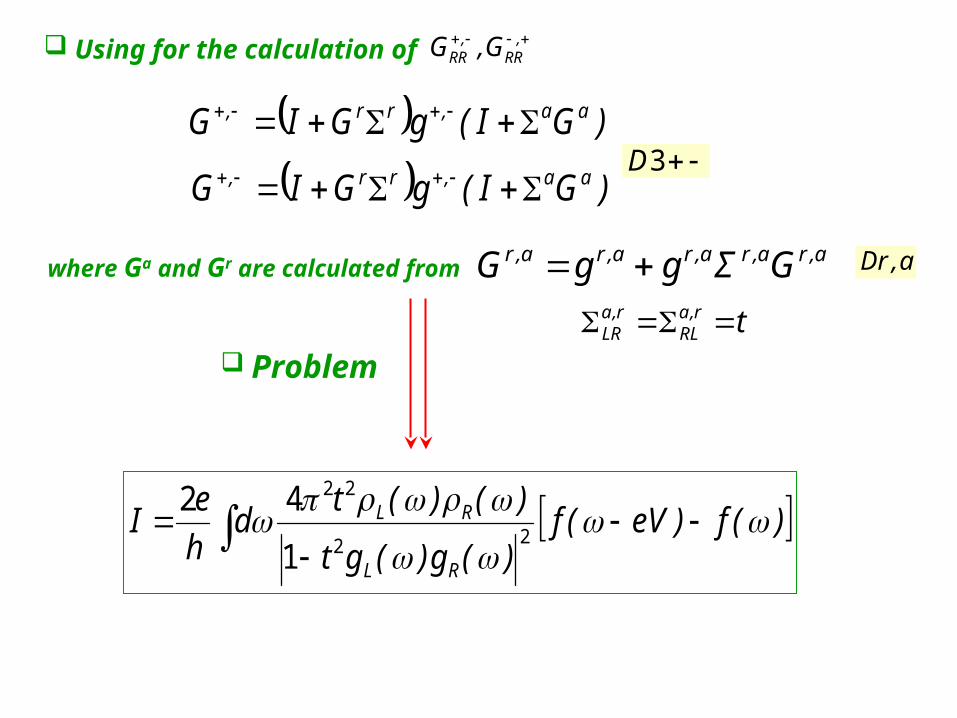
Using for the calculation of ,RR
,RR G,G
)GI(gGIG aa,rr,
3D )GI(gGIG aa,rr,
where Ga and Gr are calculated froma,ra,ra,ra,ra,r GΣggG a,Dr
tr,aRL
r,aLR
Problem
)(f)eV(f)(g)(gt
)()(td
h
eI
RL
RL
22
22
1
42
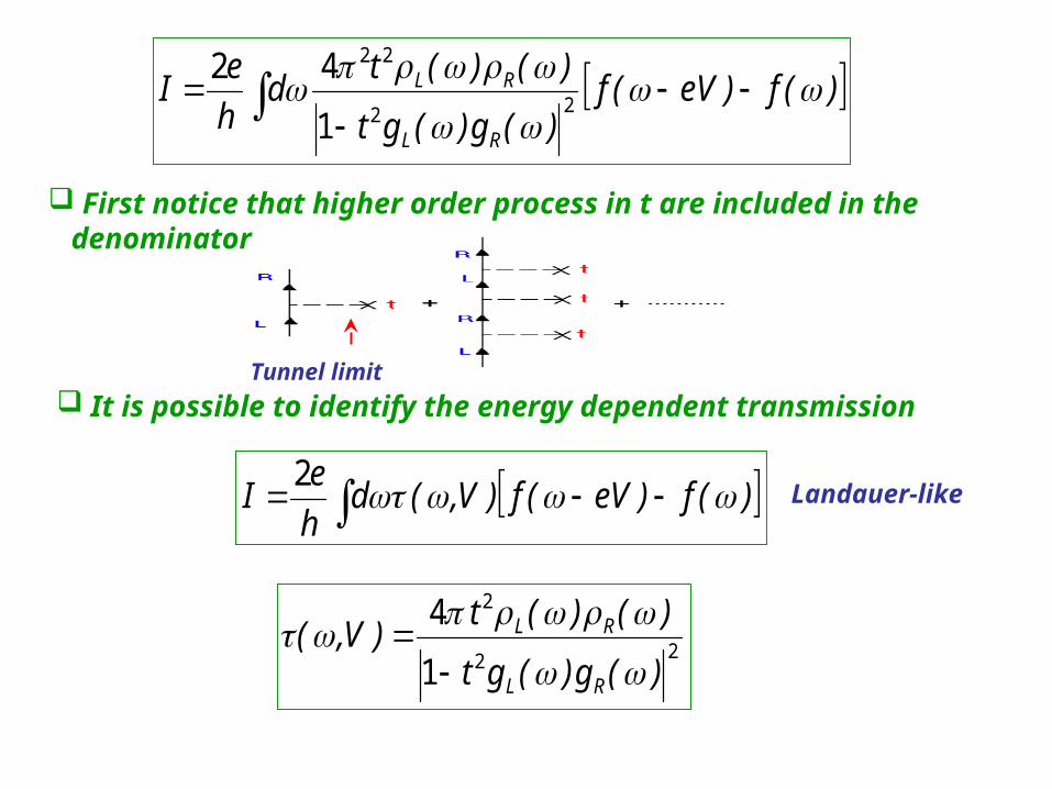
First notice that higher order process in t are included in the denominator
)(f)eV(f)(g)(gt
)()(td
h
eI
RL
RL
22
22
1
42
Tunnel limit It is possible to identify the energy dependent transmission
)(f)eV(f)V,(dh
eI 2
Landauer-like
22
2
1
4
)(g)(gt
)()(t)V,(
RL
RL
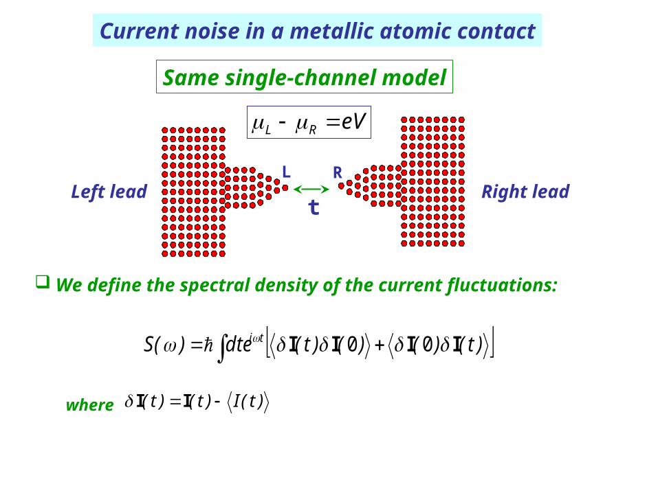
Current noise in a metallic atomic contact
Same single-channel model
L R
tLeft lead Right lead
eVRL
We define the spectral density of the current fluctuations:
)t()()()t(dte)(S ti IIII 00
where )t(I)t()t( II
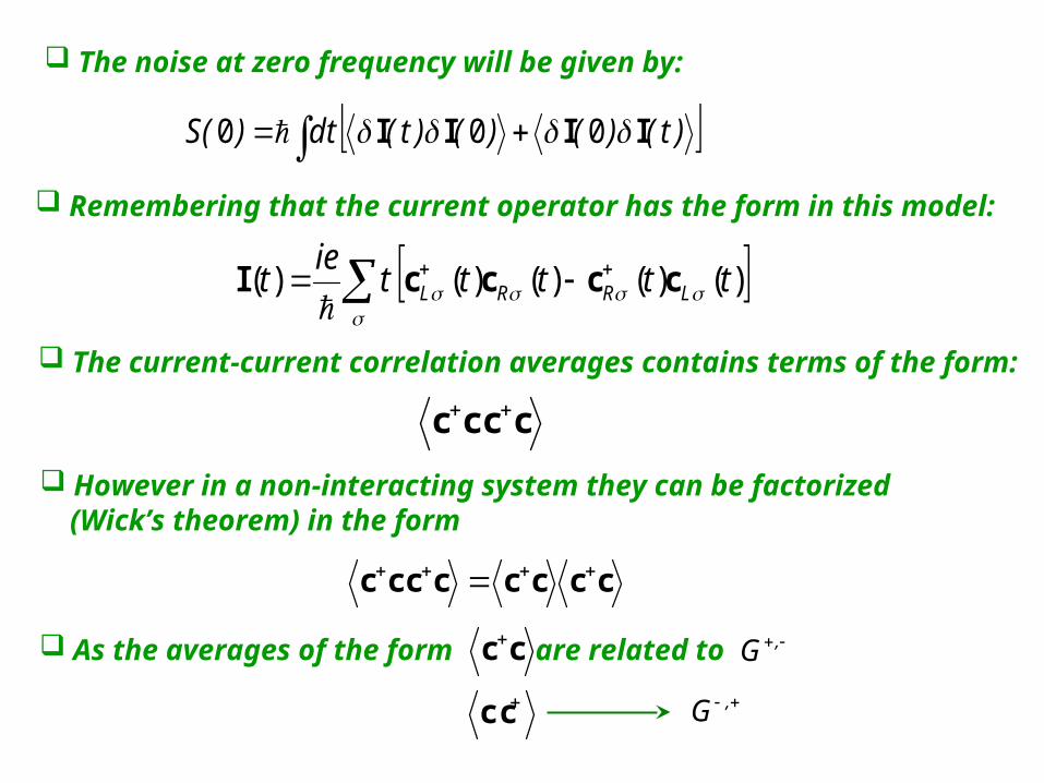
The noise at zero frequency will be given by:
)t()()()t(dt)(S IIII 000
Remembering that the current operator has the form in this model:
)()()()()( tttttie
t LRRL ccccI
The current-current correlation averages contains terms of the form:
cccc
However in a non-interacting system they can be factorized (Wick’s theorem) in the form
cccccccc
As the averages of the form are related to cc ,G
cc ,G
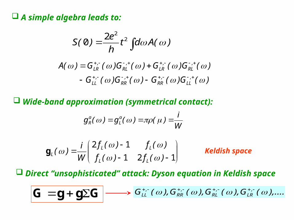
A simple algebra leads to:
)(Adth
e)(S 2
220
)(G)(G)(G)(G
)(G)(G)(G)(G)(A,LL
,RR
,RR
,LL
,RL
,LR
,RL
,LR
Wide-band approximation (symmetrical contact):
W
i)()(g)(g a
LaR
121
12
)(f)(f
)(f)(f
W
i)(
LL
LLL
g Keldish space
Direct “unsophisticated” attack: Dyson equation in Keldish space
GggG ),....(G),(G),(G),(G ,LR
,RL
,RR
,LL
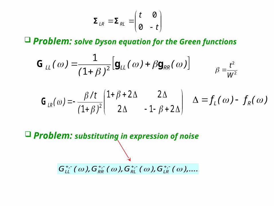
t
tRLLR 0
0ΣΣ
Problem: solve Dyson equation for the Green functions
)()()(
)( RRLLLL
ggG
21
1
212
221
1 2
)(
t/)(LRG
2
2
W
t
)(f)(f RL
),....(G),(G),(G),(G ,LR
,RL
,RR
,LL
Problem: substituting in expression of noise
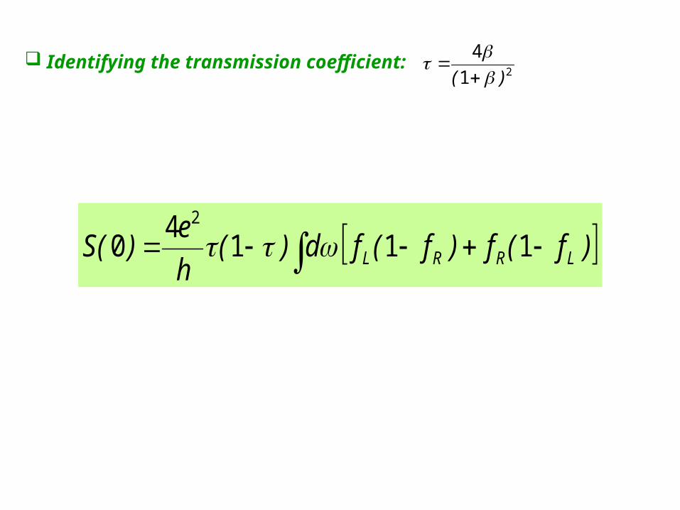
)f(f)f(fd)(h
e)(S LRRL 1114
02
Identifying the transmission coefficient: 21
4
)(
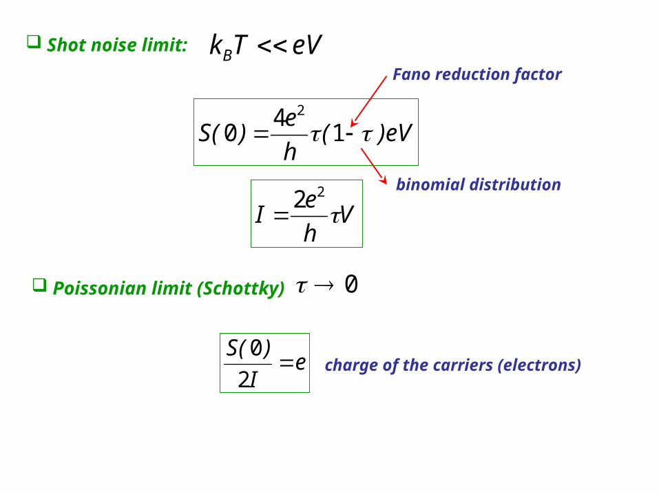
Shot noise limit: eVTkB
eV)(h
e)(S 14
02
Fano reduction factor
Poissonian limit (Schottky)
Vh
eI
22
0
eI
)(S
2
0
binomial distribution
charge of the carriers (electrons)
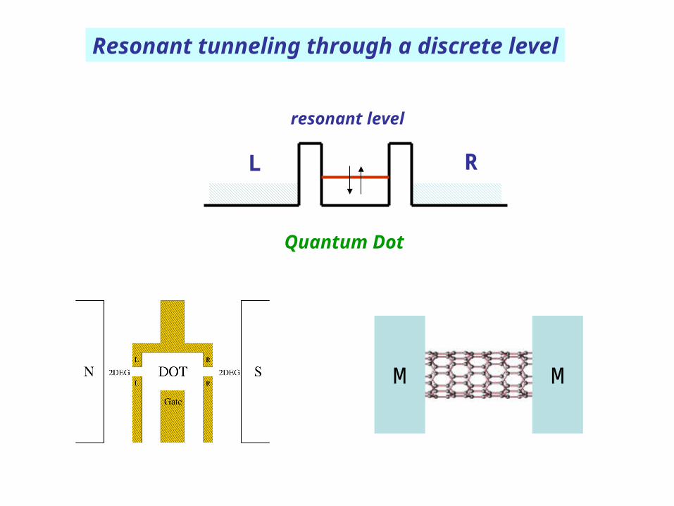
Resonant tunneling through a discrete level
resonant level
L R
Quantum Dot
M M
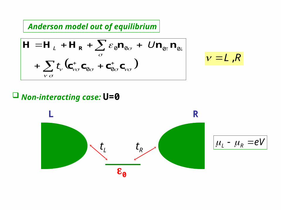
Anderson model out of equilibrium
cccc
nnnHHH R
00
0000
t
UL
RL,
Non-interacting case: U=0
0
Lt Rt
L R
eVRL
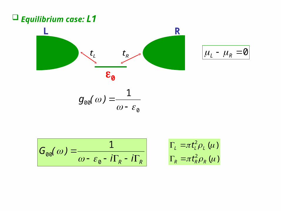
Equilibrium case: L1
RR ii)(G
000
1
0
Lt Rt
L R
0 RL
)(
)(2
2
RRR
LLL
t
t
000
1
)(g
),(),( ,0
,0 ttGttGt
eLLL
I
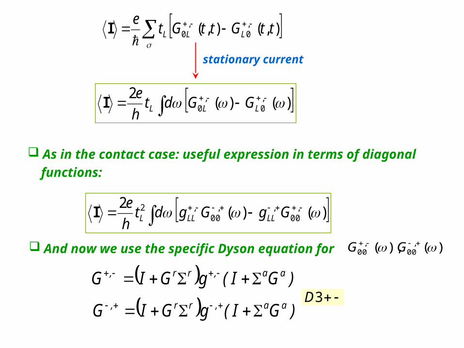
)()(2 ,
0,
0 LLL GGdth
eI
stationary current
As in the contact case: useful expression in terms of diagonal
functions:
)()(2 ,
00,,
00,2 GgGgdt
h
eLLLLLI
And now we use the specific Dyson equation for )(),( ,00
,00 GG
)GI(gGIG aa,rr,
3D )GI(gGIG aa,rr,

Problem: substitution in expression of current:
)()()()()(42 2
00222 RL
rRLRL ffGdtt
h
eI
Linear conductance
2
00222
2
)()()(42 r
RLRL Gtth
eG
As we have )(2 LLL t )(2 RRR t and
RR ii)(G
000
1
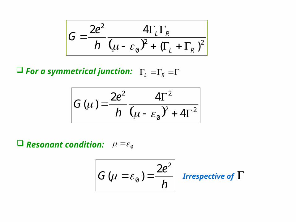
220
2
)(
42
RL
RL
h
eG
For a symmetrical junction: RL
220
22
4
42)(
h
eG
Resonant condition: 0
h
eG
2
0
2)( Irrespective of
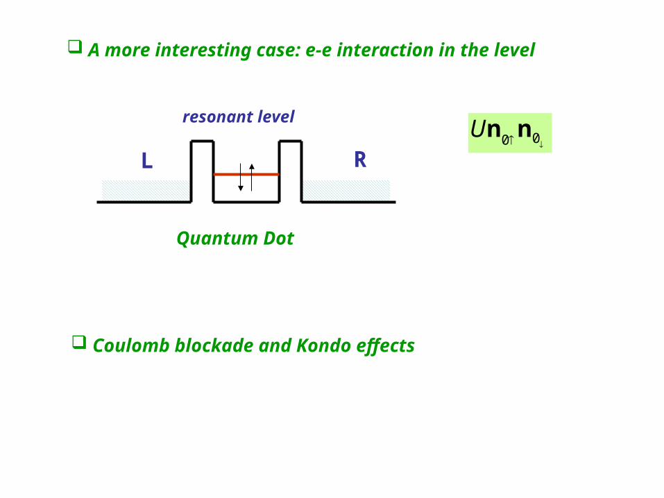
A more interesting case: e-e interaction in the level
resonant level
L R
Quantum Dot
00nnU
Coulomb blockade and Kondo effects
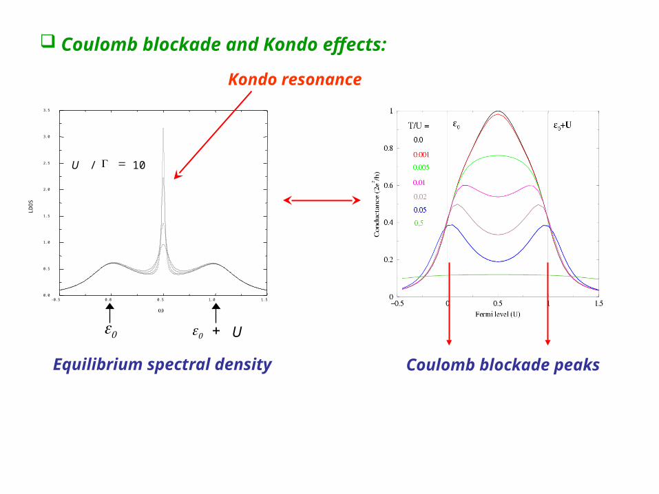
Coulomb blockade and Kondo effects:
-0.5 0.0 0.5 1.0 1.50.0
0.5
1.0
1.5
2.0
2.5
3.0
3.5
LD
OS
U / 10
U
Equilibrium spectral density Coulomb blockade peaks
Kondo resonance
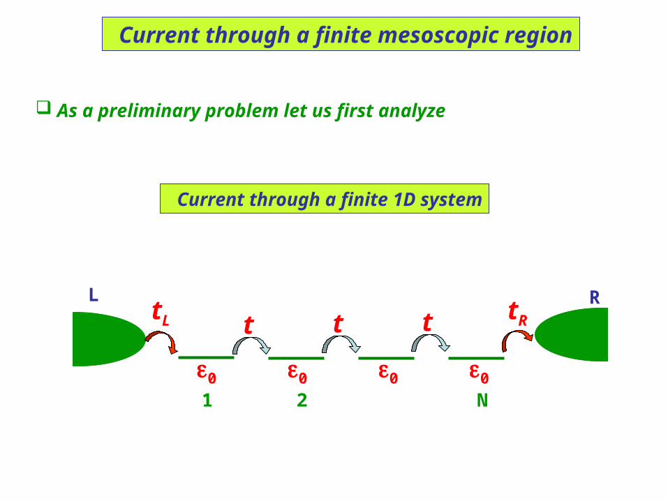
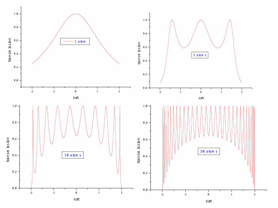
Current through a finite mesoscopic region
As a preliminary problem let us first analyze
Current through a finite 1D system
0
L R
0 0 0
t t ttL tR
1 2 N
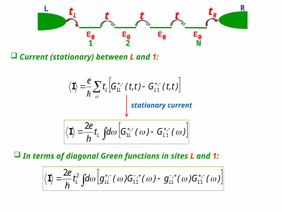
Current (stationary) between L and 1:
0
L R
0 0 0
t t ttL tR
1 2 N
)t,t(G)t,t(Gte ,
L,LL 11
I
)(G)(Gdth
e ,L
,LL 11
2I
stationary current
In terms of diagonal Green functions in sites L and 1:
)(G)(g)(G)(gdth
e ,,LL
,,LLL 1111
22I
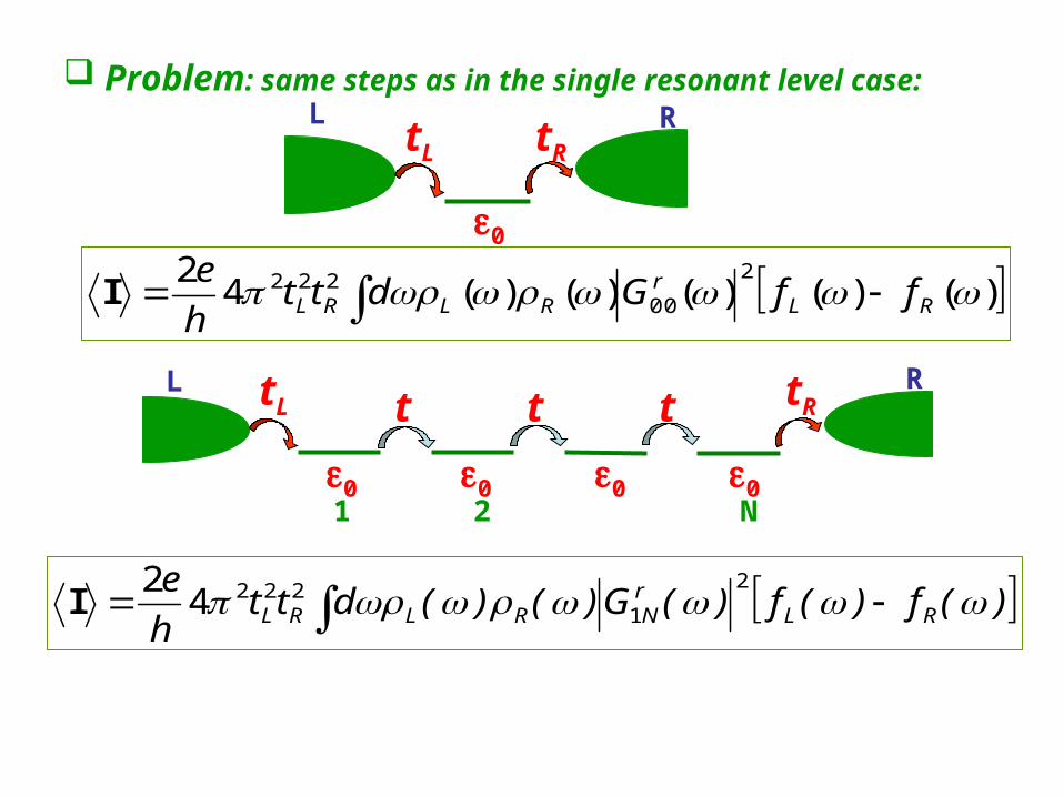
Problem: same steps as in the single resonant level case:
0
L RtL tR
)()()()()(42 2
00222 RL
rRLRL ffGdtt
h
eI
0
L R
0 0 0
t t ttL tR
1 2 N
)(f)(f)(G)()(dtth
eRL
rNRLRL
2
12224
2I
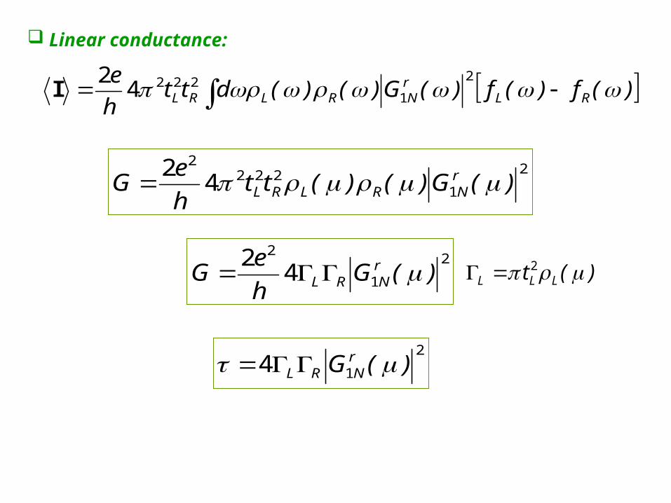
Linear conductance:
)(f)(f)(G)()(dtth
eRL
rNRLRL
2
12224
2I
2
1222
2
42
)(G)()(tth
eG r
NRLRL
2
1
2
42
)(Gh
eG r
NRL )(t LLL 2
2
14 )(G rNRL
-2 -1 0 1 2
0,0
0,2
0,4
0,6
0,8
1,0tr
ansm
issi
on
/t
1 atom
-2 -1 0 1 20,0
0,2
0,4
0,6
0,8
1,0
3 atoms
tran
smis
sion
/t
-2 -1 0 1 20,0
0,2
0,4
0,6
0,8
1,0
tran
smis
sion
/t
10 atoms
-2 -1 0 1 20,0
0,2
0,4
0,6
0,8
1,0
tra
nsm
issi
on
/t
30 atoms
L
R
eVRL
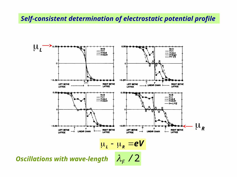
Self-consistent determination of electrostatic potential profile
Oscillations with wave-length 2/F
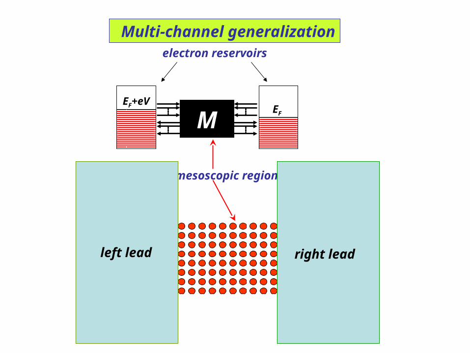
Multi-channel generalizationelectron reservoirs
EF
EF+eV
M
mesoscopic region
left lead right lead
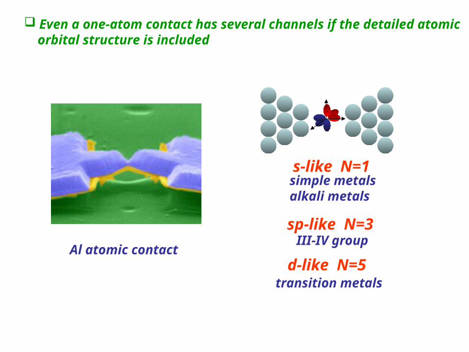
Even a one-atom contact has several channels if the detailed atomic orbital structure is included
s-like N=1simple metalsalkali metals
sp-like N=3III-IV group
d-like N=5transition metals
Al atomic contact
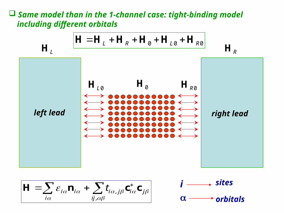
000 RLRL HHHHHH
Same model than in the 1-channel case: tight-binding model including different orbitals
left lead right lead
LH RH
0H0LH 0RH
ji,ij
j,ii
ii t ccnH i sites
orbitals
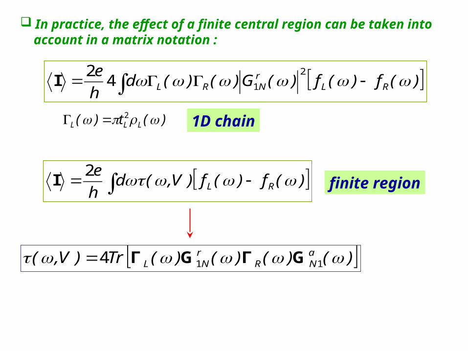
In practice, the effect of a finite central region can be taken into account in a matrix notation :
1D chain
)()()()(Tr)V,( aNR
rNL 114 GΓGΓ
)(f)(f)(G)()(dh
eRL
rNRL
2
142
I
)(t)( LLL 2
)(f)(f)V,(dh
eRL 2
I finite region
)()()()(Tr),( aNR
rNL 1140 GΓGΓ
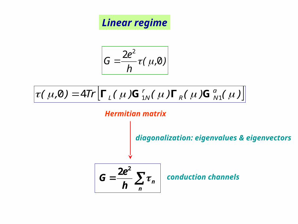
Linear regime
),(h
eG 0
2 2
Hermitian matrix
n
nh
eG
22
diagonalization: eigenvalues & eigenvectors
conduction channels
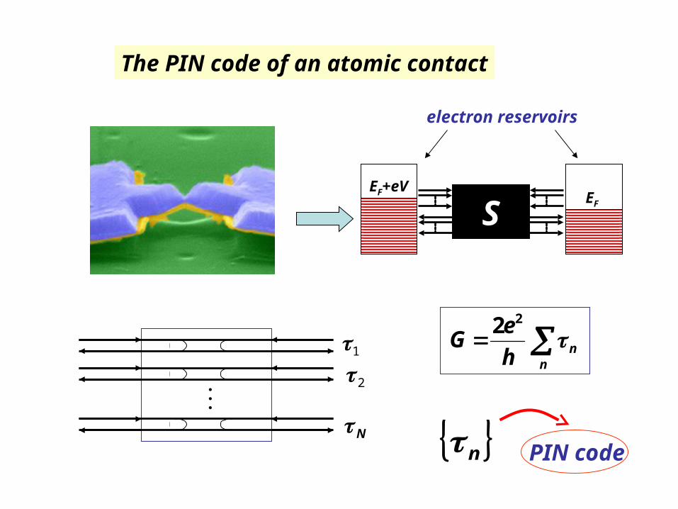
The PIN code of an atomic contact
electron reservoirs
EF
EF+eV
S
S1
2
N
n
nh
eG
22
PIN code n
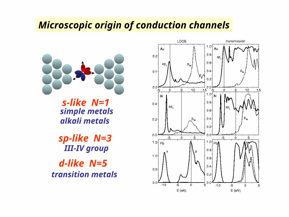
Microscopic origin of conduction channels
s-like N=1simple metalsalkali metals
sp-like N=3III-IV group
d-like N=5transition metals
Recommended