Applying the Newmark Method into the Discontinuous
Deformation Analysis
Bo Peng
Thesis submitted to the Faculty of the
Virginia Polytechnic Institute and State University
in partial fulfillment of the requirements for the degree of
Master of Science
in
Computer Science and Applications
Yang Cao
Linbing Wang
Alexey Onufriev
September 15, 2014
Blacksburg, Virginia
Keywords: Newmark method, Discontinuous deformation analysis, Rock mechanics
Copyright 2014, Bo Peng
Applying the Newmark Method into the Discontinuous Deformation Analysis
Bo Peng
(ABSTRACT)
Discontinuous deformation analysis (DDA) is a newly developed simulation method for discon-
tinuous systems. It was designed to simulate systems with arbitrary shaped blocks with high
efficiency while providing accurate solutions for energy dissipation. But DDA usually exhibits
damping effects that are inconsistent with theoretical solutions. The deep reason for these artifi-
cial damping effects has been an open question, and it is hypothesized that these damping effects
could result from the time integration scheme. In this thesis two time integration methods are
investigated: the forward Euler method and the Newmark method.
The work begins by combining the Newmark method and the DDA. An integrated Newmark
method is also developed, where velocity and acceleration do not need to be updated. In simu-
lations, two of the most widely used models are adopted to test the forward Euler method and the
Newmark method. The first one is a sliding model, in which both the forward Euler method and
the Newmark method give accurate solutions compared with analytical results. The second model
is an impacting model, in which the Newmark method has much better accuracy than the forward
Euler method, and there are minimal damping effects.

Dedication
This thesis is dedicated to my parents: Xiaochu Peng and Hongbo Tang,
iii

Acknowledgments
I would like to give my sincere gratitude to Dr. Yang Cao, who is an incredible advisor: taught
me the attitude to the research, trained me professionally, revised my thesis three times and helped
me rehearsal presentation three times. Besides, he is very caring and considerate, which helps
me make through my second degree (CS) really smoothly. My appreciation goes to Dr. Linbing
Wang in CEE department, who is my advisor in CEE department and my committee member in
CS research. He provided me great opportunities to study and research in Virginia Tech. I would
like to thank my committee member Dr. Alexey Onufriev. I cannot realize my limitation without
his help and suggestion. I also want to thank my group mates: Fei Li, Shuo Wang, Minghan Chen.
I enjoyed the friendship with you.
I want to thank my parents for their forever love and supports. I can achieve nothing without them.
I am thankful for my roommates, my dance crew mates, and my very supportive friend Cris. They
are the irreplaceable parts in my Blacksburg life.
iv
Contents
1 Introduction 1
1.1 Research Objects . . . . . . . . . . . . . . . . . . . . . . . . . . . . . . . . . . . 4
1.2 Organization . . . . . . . . . . . . . . . . . . . . . . . . . . . . . . . . . . . . . . 5
2 Background 7
2.1 Introduction to the DDA . . . . . . . . . . . . . . . . . . . . . . . . . . . . . . . 7
2.1.1 The Origin of the DDA . . . . . . . . . . . . . . . . . . . . . . . . . . . . 7
2.1.2 Time-step Loop . . . . . . . . . . . . . . . . . . . . . . . . . . . . . . . . 9
2.1.3 Interaction . . . . . . . . . . . . . . . . . . . . . . . . . . . . . . . . . . 10
2.1.4 Boundary Conditions . . . . . . . . . . . . . . . . . . . . . . . . . . . . . 10
2.1.5 Two Dimensional DDA and Three Dimensional DDA . . . . . . . . . . . . 11
2.2 Theoretical Three Dimensional DDA . . . . . . . . . . . . . . . . . . . . . . . . . 11
v
2.2.1 The Complete First Order Approximation . . . . . . . . . . . . . . . . . . 11
2.2.2 Energy Minimization and Equilibrium Equation . . . . . . . . . . . . . . . 15
2.2.3 Structure of Stiffness Matrix and Right-side Vector . . . . . . . . . . . . . 16
2.3 Previous Work on DDA Validation . . . . . . . . . . . . . . . . . . . . . . . . . . 22
2.3.1 Sliding . . . . . . . . . . . . . . . . . . . . . . . . . . . . . . . . . . . . 22
2.3.2 Energy Dissipation Model . . . . . . . . . . . . . . . . . . . . . . . . . . 26
2.4 Challenges . . . . . . . . . . . . . . . . . . . . . . . . . . . . . . . . . . . . . . . 27
3 Newmark Method in 3D-DDA 29
3.1 Newmark Method . . . . . . . . . . . . . . . . . . . . . . . . . . . . . . . . . . . 29
3.2 Newmark Method in DDA . . . . . . . . . . . . . . . . . . . . . . . . . . . . . . 31
3.3 The Energy Balance of the Newmark Method in DDA . . . . . . . . . . . . . . . . 34
3.4 The Integrated Newmark Method in DDA . . . . . . . . . . . . . . . . . . . . . . 35
4 Implement Details 39
4.1 Structure of the DDA Code . . . . . . . . . . . . . . . . . . . . . . . . . . . . . . 40
4.2 Newmark Method in the DDA Code . . . . . . . . . . . . . . . . . . . . . . . . . 43
4.3 Implement of the Integrated Newmark Method in the DDA Code . . . . . . . . . . 45
vi
5 Results and Analysis 48
5.1 Sliding Model . . . . . . . . . . . . . . . . . . . . . . . . . . . . . . . . . . . . . 49
5.1.1 Accuracy Analysis . . . . . . . . . . . . . . . . . . . . . . . . . . . . . . 51
5.1.2 Computational Time Comparison . . . . . . . . . . . . . . . . . . . . . . 54
5.2 Impacting Model . . . . . . . . . . . . . . . . . . . . . . . . . . . . . . . . . . . 55
5.2.1 Damping Effects . . . . . . . . . . . . . . . . . . . . . . . . . . . . . . . 56
5.2.2 Time-step effects . . . . . . . . . . . . . . . . . . . . . . . . . . . . . . . 58
5.3 Summary . . . . . . . . . . . . . . . . . . . . . . . . . . . . . . . . . . . . . . . 64
6 Conclusion and Future Work 65
Bibliography 67
vii
List of Figures
1.1 Left: Individual aggregates in DEM. Right: DEM simulation for aggregates
in asphalt binder. . . . . . . . . . . . . . . . . . . . . . . . . . . . . . . . . . . 3
1.2 Left:irregular shaped blocks in the DDA simulation. Right: The DDA slope
stability analysis for Bai He Tan Hydropower station. . . . . . . . . . . . . . 4
2.1 DDA simulation for unstable rocks in a tunnel . . . . . . . . . . . . . . . . . . 9
2.2 The sliding model . . . . . . . . . . . . . . . . . . . . . . . . . . . . . . . . . . 24
2.3 Left: Single sliding face in 3D. Right: Double sliding face in 3D. . . . . . . . 25
2.4 Initial position for filling rock tests. . . . . . . . . . . . . . . . . . . . . . . . . 26
4.1 Flowchart for the DDA code . . . . . . . . . . . . . . . . . . . . . . . . . . . . 42
4.2 Switch between the forward Euler method and the Newmark method . . . . 46
4.3 Flowchart for GXSTIFF() function in DDA code . . . . . . . . . . . . . . . . . 47
viii
5.1 Sliding model: a small block sliding along a fixed slope . . . . . . . . . . . . 50
5.2 Displacement-time relationship for the sliding model. With size of timestep
0.002s, both the forward Euler method and the Newmark method provide
solutions very close to the analytical solution. . . . . . . . . . . . . . . . . . . 52
5.3 Relative error and time relationship for the sliding model. The relative errors
of both the Newmark method and the forward Euler method decline steadily
after a point. . . . . . . . . . . . . . . . . . . . . . . . . . . . . . . . . . . . . . 53
5.4 Time-step size and relative error relatioship for the sliding model. The com-
parison is based on simulation solutions which have the same simulatation
time (1.5 s) . . . . . . . . . . . . . . . . . . . . . . . . . . . . . . . . . . . . . . 53
5.5 Model size (timestep number) and computational costs relationship in slid-
ing model. The computational time for the Newmark method and the for-
ward Euler method are almost the same. . . . . . . . . . . . . . . . . . . . . 54
5.6 Impacting model: a small block falling down and constantly impacting a
fixed block . . . . . . . . . . . . . . . . . . . . . . . . . . . . . . . . . . . . . . 56
5.7 Comparison of displacement between the Newmark method, the forward
Euler method and the analytical solution in the impacting model. With a
time-step size 0.002(s), the forward Eular method shows strong damping
effects; the classic Newmark method illustrates a good match with analyti-
cal solution; and the integrated Newmark method has an amplifed effects. . 59
ix
5.8 Comparison of velocity between the Newmark method, forward Euler method
and analytical solution in the impacting model. . . . . . . . . . . . . . . . . . 59
5.9 Comparison of acceleration between the Newmark method and forward
Euler method in the impacting model. . . . . . . . . . . . . . . . . . . . . . . 60
5.10 Comparison of energy between the Newmark method and forward Euler
method in the impacting model. . . . . . . . . . . . . . . . . . . . . . . . . . . 60
5.11 Comparison of displacement from the Newmark method, the forward Eu-
ler method and the analytical solution in impacting model with time-step
0.0005(s). . . . . . . . . . . . . . . . . . . . . . . . . . . . . . . . . . . . . . . 61
5.12 Comparison of displacement from the Newmark method, the forward Eu-
ler method and the analytical solution in impacting model whose time-step
equals to 0.0015(s). . . . . . . . . . . . . . . . . . . . . . . . . . . . . . . . . . 62
5.13 Comparison of displacement from the Newmark method, the forward Eu-
ler method and the analytical solution in impacting model whose time-step
equals to 0.004(s). . . . . . . . . . . . . . . . . . . . . . . . . . . . . . . . . . 62
5.14 The relationship between Relative error and time-step in impacting model
using Newmark method and forward Euler method. . . . . . . . . . . . . . . 63
5.15 The relationship between energy relative error and time-step in impacting
model using Newmark method and forward Euler method. . . . . . . . . . . 63
x
Chapter 1
Introduction
Rock, as a widely existing material in nature, is closely related to our daily life: falling rocks near
highway might result in serious accidents; slope stability is one of the key factors to ensure safety
of construction activities on either man-made or natural slops. From irregular aggregates to huge
rock mountains, rock systems are highly discrete. Therefore, it is very important to develop models
and simulation methods to help us understand discrete rock systems.
There are several popular simulation methods to simulate the dynamic behavior of rock systems,
such as the finite element method (FEM), the discontinuous deformation analysis (DDA) and the
discrete element methods (DEM). In these three methods, the FEM is mainly used for continuous
problems, while the DDA and the DEM are designed for discrete systems.
The finite element method (FEM) is a popular simulation method to simulate mechanical sys-
tems5, 6 . However, in terms of discontinuous materials, especially for blocky systems, the FEM is
1
Bo Peng Chapter 1. Introduction 2
highly restricted when solving big deformation problems, while discrete methods (e.g. DDA and
DEM) do not have this shortcoming.
The discrete element method (DEM), first proposed by Cundall in 1979,7 has been developed
rapidly worldwide since then. The DEM can be applied in a wide range of research areas, including
the particle fluidization of cohesionless and cohesive particle flow, confined or unconfined particle
flow, particle flow in hoppers, in mixers, in drums and mills, particle packing, compaction of
particles, etc. The advantage of the DEM is that it can simulate heterogeneity materials through
discretization. Setting different parameters to the contributing materials in the simulation helps
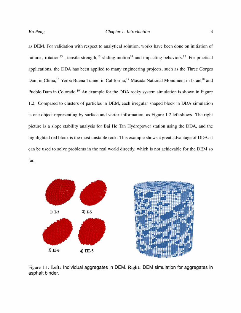
to distinguish their interaction. An example of the DEM asphalt binder simulation with irregular
shaped aggregates is shown in Figure 1.1. In the simulation two different materials, aggregates
and asphalt, were developed in the same specimen, and clumps of particles were used to simulate
irregular shaped aggregates. Although DEM is design for discrete systems, it has defects such as
inaccurate artificial energy dissipation estimation and not sophisticated contact interaction models.
Therefore, the DEM is restricted in particle flow problems.
The discontinuous deformation analysis (DDA) was first proposed by Shi in 1988.8 Because of
its advantages such as high accuracy, reasonable contact interaction model, relatively low com-
putational cost etc., the DDA shows great potential to be a powerful tool for simulating discrete
rock systems. Besides the original two-dimensional DDA, some extended methods are developed,
including the backward DDA,9 the particle DDA,10 the manifold method,11 and the three dimen-
sional DDA.12 Validation results for DDA are obtained from comparison between DDA results and
analytical solution, laboratory data, field data, and results of other discrete element analysis, such
Bo Peng Chapter 1. Introduction 3
as DEM. For validation with respect to analytical solution, works have been done on initiation of
failure , rotation13 , tensile strength,13 sliding motion14 and impacting behaviors.15 For practical
applications, the DDA has been applied to many engineering projects, such as the Three Gorges
Dam in China,16 Yerba Buena Tunnel in California,17 Masada National Monument in Israel18 and
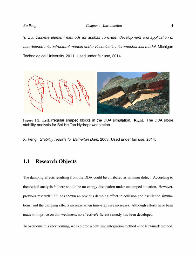
Pueblo Dam in Colorado.19 An example for the DDA rocky system simulation is shown in Figure
1.2. Compared to clusters of particles in DEM, each irregular shaped block in DDA simulation
is one object representing by surface and vertex information, as Figure 1.2 left shows. The right
picture is a slope stability analysis for Bai He Tan Hydropower station using the DDA, and the
highlighted red block is the most unstable rock. This example shows a great advantage of DDA: it
can be used to solve problems in the real world directly, which is not achievable for the DEM so
far.
Figure 1.1: Left: Individual aggregates in DEM. Right: DEM simulation for aggregates inasphalt binder.
Bo Peng Chapter 1. Introduction 4
Y. Liu, Discrete element methods for asphalt concrete: development and application of
userdefined microstructural models and a viscoelastic micromechanical model. Michigan
Technological University, 2011. Used under fair use, 2014.
Figure 1.2: Left:irregular shaped blocks in the DDA simulation. Right: The DDA slopestability analysis for Bai He Tan Hydropower station.
X. Peng, Stability reports for Baiheitan Dam, 2003. Used under fair use, 2014.
1.1 Research Objects
The damping effects resulting from the DDA could be attributed as an inner defect. According to
theoretical analysis,20 there should be no energy dissipation under undamped situation. However,
previous research4, 15, 21 has shown an obvious damping effect in collision and oscillation simula-
tions, and the damping effects increase when time-step size increases. Although efforts have been
made to improve on this weakness, no effective/efficient remedy has been developed.
To overcome this shortcoming, we explored a new time integration method – the Newmark method,
Bo Peng Chapter 1. Introduction 5
and applied it to the DDA code. As mentioned above, the DDA is designed to simulate displace-
ment changes with respect to time. For the velocity and acceleration information in the stiffness
matrix, the global equation of the DDA can be formulated as a set of ordinary differential equa-
tions (ODEs). However, the swift changes of contact status cause the stiffness matrix in the ODEs
to vary frequently. As a result, it is very inefficient to apply traditional ODE solvers to solve the
global equation in the DDA. Therefore, highly discrete time integration methods must be applied
to the DDA.
Prior to this work, only the forward Euler method was applied to DDA. In this thesis,the Newmark
method is used as a time integration scheme in the DDA for the first time. A comprehensive
comparison between the forward Euler method and the Newmark method when applied in the
DDA will be studied based on two test models: a sliding model and an impacting model. These
two models are the most basic testing models for the DDA method, because both models involve
simulations of block contacting in both tangential and normal directions.
1.2 Organization
The main goal of research in this thesis is to improve the simulation accuracy of DDA through
the Newmark method. The structure of this thesis is organized as following: Chapter two will
give a brief description on the DDA theory and the research literature of DDA. Chapter three
will introduce the application of the Newmark method in DDA, as well as an integrated Newmark
method. Chapter four is going to illustrate the implement details, including the DDA code structure
Bo Peng Chapter 1. Introduction 6
and how to combine the Newmark method into DDA. Chapter five shows a comprehensive data
analysis of the Newmark simulation. The results are compared to the traditional forward Euler
simulation. Chapter six presents the conclusion of this thesis and proposes the future work to
search for optimized parameters.
Chapter 2
Background
2.1 Introduction to the DDA
2.1.1 The Origin of the DDA
Before the description of the DDA, two basic rock definitions need to be introduced as below:
• Structure plane: there are geological surfaces with different factors and traits in rocks; such
as joint, fracture, fault. Because of their existence, rock can not be considered as continuous
material: rocks are split into irregular rock blocks. The interface separating rocks is called
structure plane. Structure interfaces are with multiple scales of sizes and properties: some
of them are big enough to present across the entire rock, while some others can not even
be seen in the surface. With the tectonic movements for billions of years, there are a huge
7

Bo Peng Chapter 2. Background 8
amount of structure planes in rocks.
• Blocky system: intricate structure planes split rock mountain into many irregular rock blocks,
which form blocky systems.
Because of the extreme anisotropy and its much lower strength than rock, structure plane is the
place that material failure occurs most. The failure mode and movement mode vary tremendously
with changes of structure planes.
With the understanding that structure planes play a key role in rock mechanics, the DDA considers
each block as an individual object, and blocks interact with each other through contact forces.
These properties of DDA simplify complicated blocky systems and their mechanical analysis,
which make the simulation of complex blocky systems possible.
DDA Problem
Considering a practical engineering project: a tunnel is planed to be built across a rock mountain.
Though the mountain is split by structure planes into large amount of individual rock blocks, it
is stable before the tunnel is developed. However, a tunnel will change the structure stability of
a mountain: rocks near the tunnel will lose some of their supports, and this will result in serious
potential risks such as falling rocks. Therefore, it is very important to know how a tunnel influences
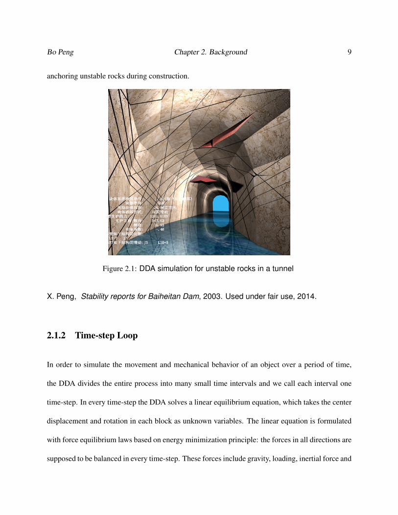
the mountain stability. Figure 2.1 shows an example of tunnel stability analysis. Through DDA
simulation, we know the information of unstable rocks, highlighted red block in picture, resulting
from tunnel excavation. With these information, the tunnel can be stabilized through actions of
Bo Peng Chapter 2. Background 9
anchoring unstable rocks during construction.
Figure 2.1: DDA simulation for unstable rocks in a tunnel
X. Peng, Stability reports for Baiheitan Dam, 2003. Used under fair use, 2014.
2.1.2 Time-step Loop
In order to simulate the movement and mechanical behavior of an object over a period of time,
the DDA divides the entire process into many small time intervals and we call each interval one
time-step. In every time-step the DDA solves a linear equilibrium equation, which takes the center
displacement and rotation in each block as unknown variables. The linear equation is formulated
with force equilibrium laws based on energy minimization principle: the forces in all directions are
supposed to be balanced in every time-step. These forces include gravity, loading, inertial force and
Bo Peng Chapter 2. Background 10
other contacting forces. More details of equation formation in the DDA will be introduced in the
next section. After solving the linear equation, we obtain the increment of displacement for each
block in the current time-step. Then according to movement laws, the velocity and acceleration
in the current step are acquired. Also, with the help of shape functions (relationship with center
displacement and displacement of arbitrary points in the block), the coordinates of blocks’ vertex
can be obtained, as well as the positions of blocks. Based on those position information, the contact
information will be determined. A time-step simulation is finished at this point, and this process
will repeat until the simulation ends.
2.1.3 Interaction
In discrete blocky systems, blocks interact with each other through contacting. There are two types
of contacting: vertex-plane contacts and edge-edge contacts. A contact is defined as the overlap
between two blocks. After a contact is formed, the two blocks are considered as being connected
with two springs: a normal spring and a tangential spring. The magnitude of spring forces is linear
with the depth of the overlap, and the spring forces will be added to the linear equilibrium equation
mentioned above.
2.1.4 Boundary Conditions
Boundary conditions in blocky systems are constrains. There are three different kinds of restric-
tions: rotation constrains, translation constrains and fixed constrains. The setting of boundary
Bo Peng Chapter 2. Background 11
conditions in the DDA is similar to that in the FEM: defining boundary conditions according to the
system structure, and adding those information into the linear equilibrium equation.
2.1.5 Two Dimensional DDA and Three Dimensional DDA
When Dr. Shi proposed the DDA method for the first time, it was designed only for two-dimensional
problems. For two dimensional DDA (2D-DDA),8 there are only three basic unknown variables
for each block: translation displacements in the X,Y directions and the rotation in the XY plane.
After the three dimensional DDA (3D-DDA) was proposed in 2001,12 the number of basic un-
known variables extended to six: displacements in X,Y,Z directions and rotations in XY, YZ, XZ
planes. With the 3D-DDA solution, it is possible to simulate all different types of movements. The
unknown variables can also include the strain information as we will illustrate in the next.
2.2 Theoretical Three Dimensional DDA
This section is based on the 2D-DDA and 3D-DDA theoretical work done by Shi.8, 12
2.2.1 The Complete First Order Approximation
Assume that a block, whose center is (x0, y0, z0), has constant strain and stress. In the following
we will demonstrate that the displacement (u, v, w) for an arbitrary point (x, y, z) in the block can
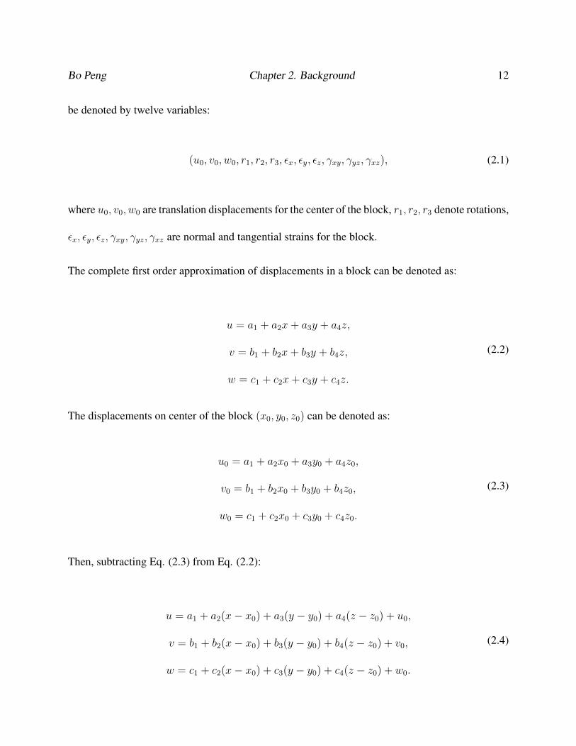
Bo Peng Chapter 2. Background 12
be denoted by twelve variables:
(u0, v0, w0, r1, r2, r3, εx, εy, εz, γxy, γyz, γxz), (2.1)
where u0, v0, w0 are translation displacements for the center of the block, r1, r2, r3 denote rotations,
εx, εy, εz, γxy, γyz, γxz are normal and tangential strains for the block.
The complete first order approximation of displacements in a block can be denoted as:
u = a1 + a2x+ a3y + a4z,
v = b1 + b2x+ b3y + b4z,
w = c1 + c2x+ c3y + c4z.
(2.2)
The displacements on center of the block (x0, y0, z0) can be denoted as:
u0 = a1 + a2x0 + a3y0 + a4z0,
v0 = b1 + b2x0 + b3y0 + b4z0,
w0 = c1 + c2x0 + c3y0 + c4z0.
(2.3)
Then, subtracting Eq. (2.3) from Eq. (2.2):
u = a1 + a2(x− x0) + a3(y − y0) + a4(z − z0) + u0,
v = b1 + b2(x− x0) + b3(y − y0) + b4(z − z0) + v0,
w = c1 + c2(x− x0) + c3(y − y0) + c4(z − z0) + w0.
(2.4)
Bo Peng Chapter 2. Background 13
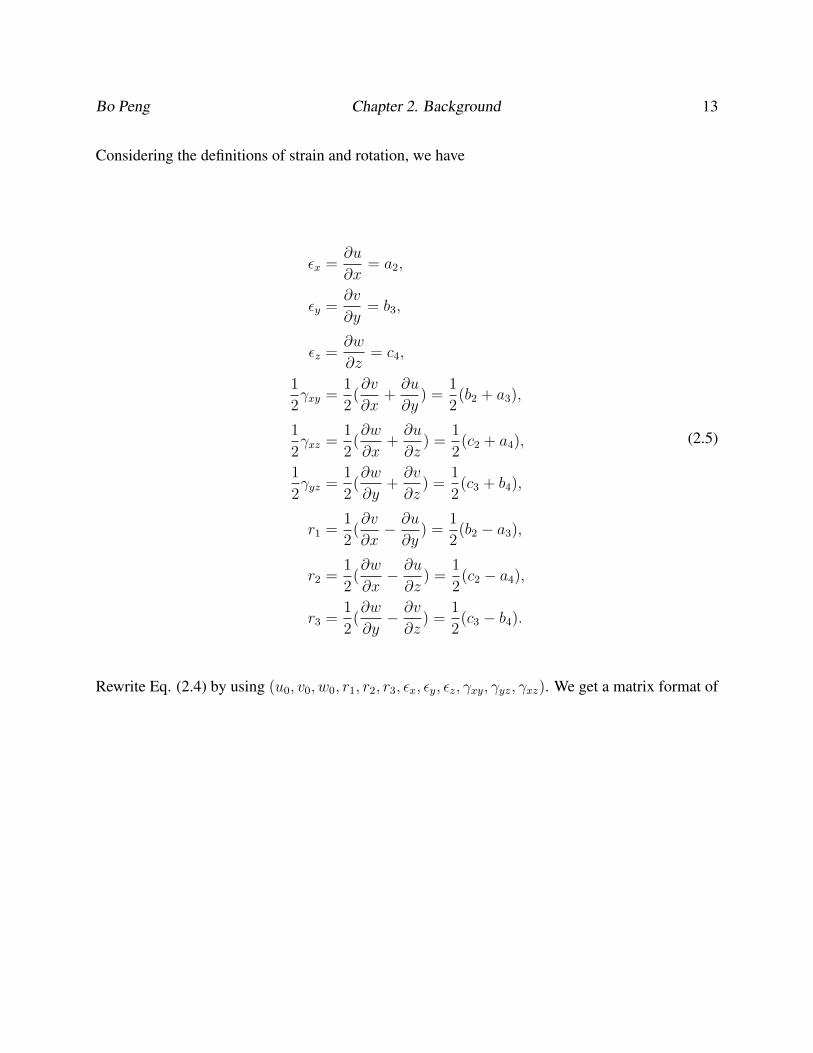
Considering the definitions of strain and rotation, we have
εx =∂u
∂x= a2,
εy =∂v
∂y= b3,
εz =∂w
∂z= c4,
1
2γxy =
1
2(∂v
∂x+∂u
∂y) =
1
2(b2 + a3),
1
2γxz =
1
2(∂w
∂x+∂u
∂z) =
1
2(c2 + a4),
1
2γyz =
1
2(∂w
∂y+∂v
∂z) =
1
2(c3 + b4),
r1 =1
2(∂v
∂x− ∂u
∂y) =
1
2(b2 − a3),
r2 =1
2(∂w
∂x− ∂u
∂z) =
1
2(c2 − a4),
r3 =1
2(∂w
∂y− ∂v
∂z) =
1
2(c3 − b4).
(2.5)
Rewrite Eq. (2.4) by using (u0, v0, w0, r1, r2, r3, εx, εy, εz, γxy, γyz, γxz). We get a matrix format of
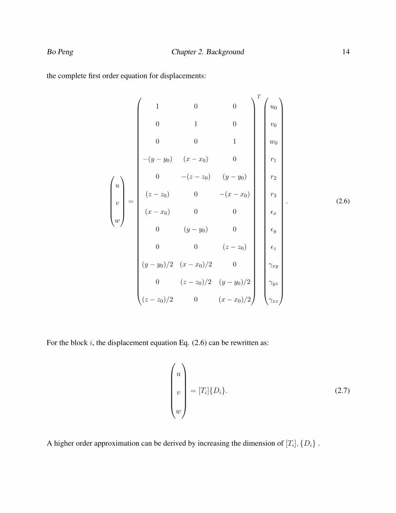
Bo Peng Chapter 2. Background 14
the complete first order equation for displacements:
u
v
w
=
1 0 0
0 1 0
0 0 1
−(y − y0) (x− x0) 0
0 −(z − z0) (y − y0)
(z − z0) 0 −(x− x0)
(x− x0) 0 0
0 (y − y0) 0
0 0 (z − z0)
(y − y0)/2 (x− x0)/2 0
0 (z − z0)/2 (y − y0)/2
(z − z0)/2 0 (x− x0)/2
T
u0
v0
w0
r1
r2
r3
εx
εy
εz
γxy
γyz
γxz
. (2.6)
For the block i, the displacement equation Eq. (2.6) can be rewritten as:
u
v
w
= [Ti]{Di}. (2.7)
A higher order approximation can be derived by increasing the dimension of [Ti], {Di} .
Bo Peng Chapter 2. Background 15
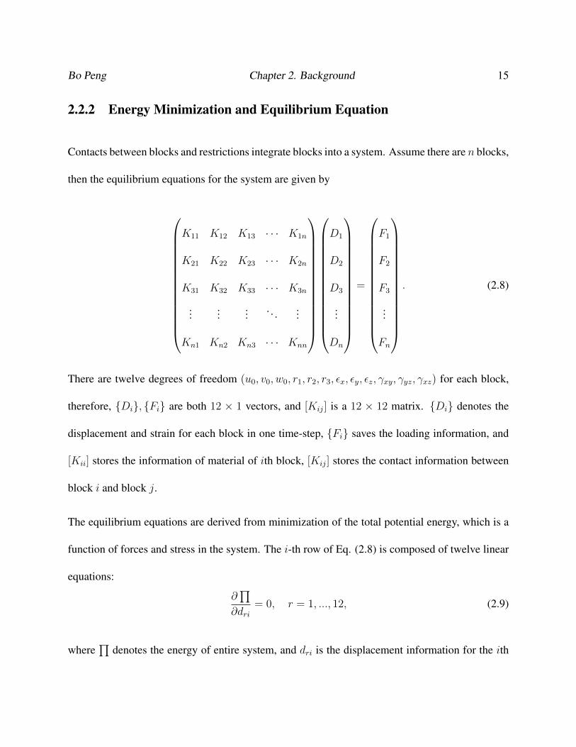
2.2.2 Energy Minimization and Equilibrium Equation
Contacts between blocks and restrictions integrate blocks into a system. Assume there are n blocks,
then the equilibrium equations for the system are given by
K11 K12 K13 · · · K1n
K21 K22 K23 · · · K2n
K31 K32 K33 · · · K3n
......
... . . . ...
Kn1 Kn2 Kn3 · · · Knn
D1
D2
D3
...
Dn
=
F1
F2
F3
...
Fn
. (2.8)
There are twelve degrees of freedom (u0, v0, w0, r1, r2, r3, εx, εy, εz, γxy, γyz, γxz) for each block,
therefore, {Di}, {Fi} are both 12 × 1 vectors, and [Kij] is a 12 × 12 matrix. {Di} denotes the
displacement and strain for each block in one time-step, {Fi} saves the loading information, and
[Kii] stores the information of material of ith block, [Kij] stores the contact information between
block i and block j.
The equilibrium equations are derived from minimization of the total potential energy, which is a
function of forces and stress in the system. The i-th row of Eq. (2.8) is composed of twelve linear
equations:
∂∏
∂dri= 0, r = 1, ..., 12, (2.9)
where∏
denotes the energy of entire system, and dri is the displacement information for the ith
Bo Peng Chapter 2. Background 16
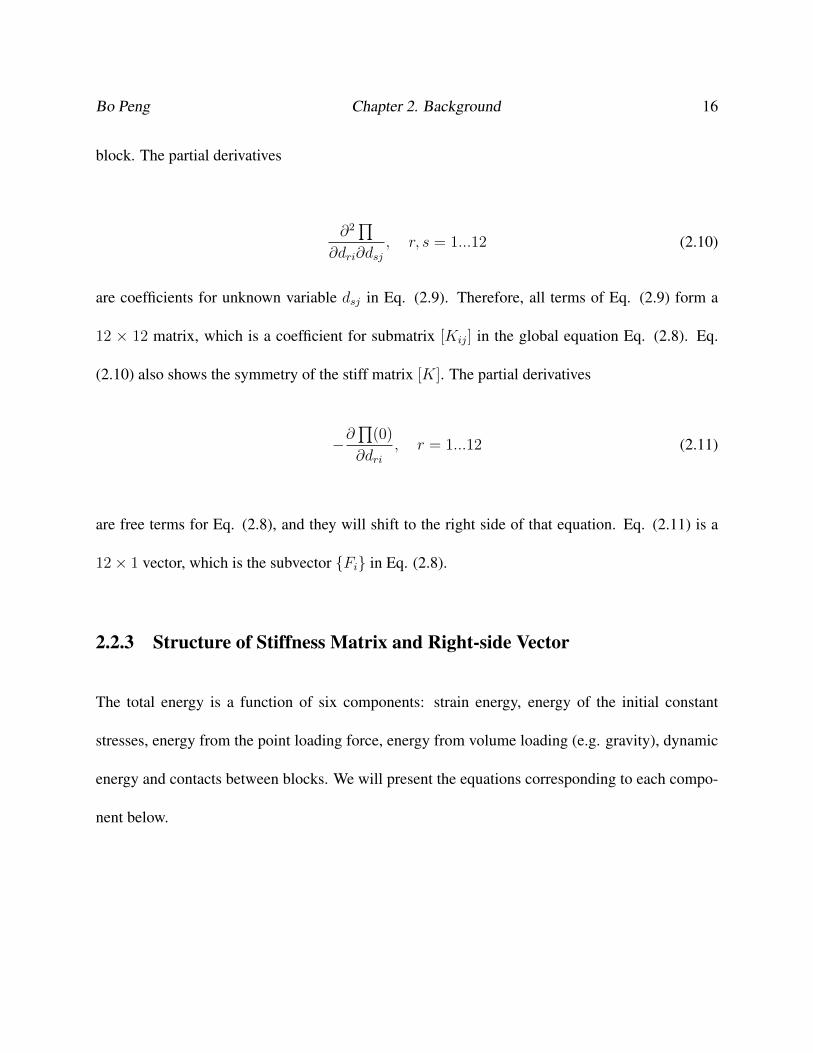
block. The partial derivatives
∂2∏
∂dri∂dsj, r, s = 1...12 (2.10)
are coefficients for unknown variable dsj in Eq. (2.9). Therefore, all terms of Eq. (2.9) form a
12 × 12 matrix, which is a coefficient for submatrix [Kij] in the global equation Eq. (2.8). Eq.
(2.10) also shows the symmetry of the stiff matrix [K]. The partial derivatives
−∂∏
(0)
∂dri, r = 1...12 (2.11)
are free terms for Eq. (2.8), and they will shift to the right side of that equation. Eq. (2.11) is a
12× 1 vector, which is the subvector {Fi} in Eq. (2.8).
2.2.3 Structure of Stiffness Matrix and Right-side Vector
The total energy is a function of six components: strain energy, energy of the initial constant
stresses, energy from the point loading force, energy from volume loading (e.g. gravity), dynamic
energy and contacts between blocks. We will present the equations corresponding to each compo-
nent below.
Bo Peng Chapter 2. Background 17
Stiffness Submatrix
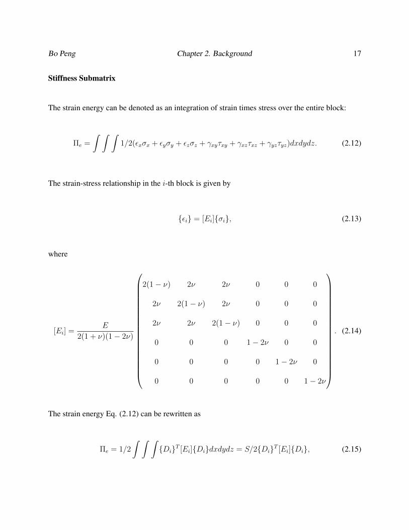
The strain energy can be denoted as an integration of strain times stress over the entire block:
Πe =
∫ ∫ ∫1/2(εxσx + εyσy + εzσz + γxyτxy + γxzτxz + γyzτyz)dxdydz. (2.12)
The strain-stress relationship in the i-th block is given by
{εi} = [Ei]{σi}, (2.13)
where
[Ei] =E
2(1 + ν)(1− 2ν)
2(1− ν) 2ν 2ν 0 0 0
2ν 2(1− ν) 2ν 0 0 0
2ν 2ν 2(1− ν) 0 0 0
0 0 0 1− 2ν 0 0
0 0 0 0 1− 2ν 0
0 0 0 0 0 1− 2ν
. (2.14)
The strain energy Eq. (2.12) can be rewritten as
Πe = 1/2
∫ ∫ ∫{Di}T [Ei]{Di}dxdydz = S/2{Di}T [Ei]{Di}, (2.15)
Bo Peng Chapter 2. Background 18
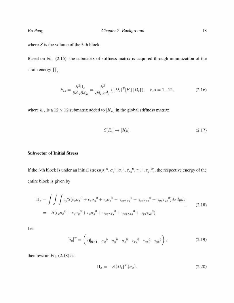
where S is the volume of the i-th block.
Based on Eq. (2.15), the submatrix of stiffness matrix is acquired through minimization of the
strain energy∏
e:
krs =∂2Πe
∂dri∂dsi=
∂2
∂dri∂dsi({Di}T [Ei]{Di}), r, s = 1...12, (2.16)
where krs is a 12× 12 submatrix added to [Kii] in the global stiffness matrix:
S[Ei]→ [Kii]. (2.17)
Subvector of Initial Stress
If the i-th block is under an initial stress(σx0, σy0, σz0, τxy0, τxz0, τyz0), the respective energy of the
entire block is given by
Πσ =
∫ ∫ ∫1/2(εxσx
0 + εyσy0 + εzσz
0 + γxyτxy0 + γxzτxz
0 + γyzτyz0)dxdydz
= −S(εxσx0 + εyσy
0 + εzσz0 + γxyτxy
0 + γxzτxz0 + γyzτyz
0)
. (2.18)
Let
[σ0]T =
([0]6×1 σx
0 σy0 σz
0 τxy0 τxz
0 τyz0
), (2.19)
then rewrite Eq. (2.18) as
Πσ = −S{Di}T{σ0}. (2.20)
Bo Peng Chapter 2. Background 19
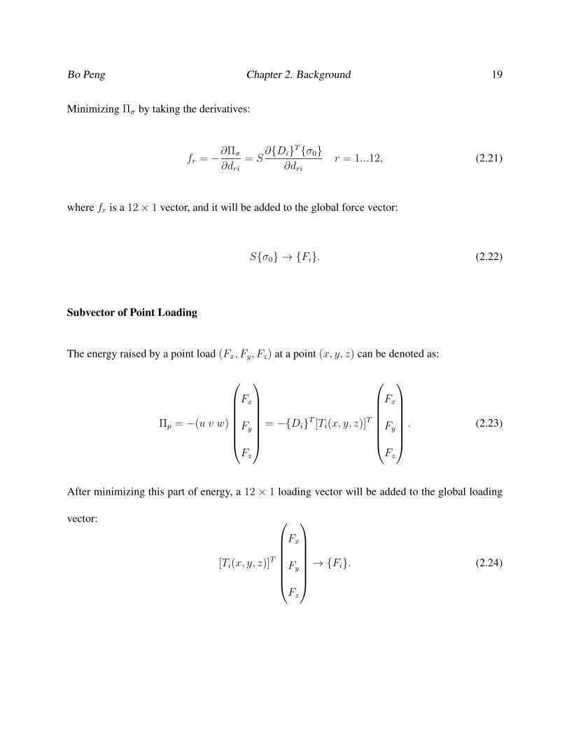
Minimizing Πσ by taking the derivatives:
fr = −∂Πσ
∂dri= S
∂{Di}T{σ0}∂dri
r = 1...12, (2.21)
where fr is a 12× 1 vector, and it will be added to the global force vector:
S{σ0} → {Fi}. (2.22)
Subvector of Point Loading
The energy raised by a point load (Fx, Fy, Fz) at a point (x, y, z) can be denoted as:
Πp = −(u v w)
Fx
Fy
Fz
= −{Di}T [Ti(x, y, z)]T
Fx
Fy
Fz
. (2.23)
After minimizing this part of energy, a 12 × 1 loading vector will be added to the global loading
vector:
[Ti(x, y, z)]T
Fx
Fy
Fz
→ {Fi}. (2.24)
Bo Peng Chapter 2. Background 20
Subvector of Volume Load
Assume that (fx, fy, fz) is a volume load applied on the ith block, then the potential energy from
the volume load is:
Πs = −∫ ∫ ∫
(u v w)
fx
fy
fz
dx dy dz = −{Di}T∫ ∫ ∫
[Ti]Tdx dy dz
fx
fy
fz
. (2.25)
Assume the center of mass for the ith block is (x0, y0, z0). Then we can rewrite Eq. (2.25) as:
Πs = −{Di}(fxS fyS fzS [0]9×1
). (2.26)
After minimizing the energy equation Eq. (2.26), the subvector of volume loading is formulated
as: (fxS fyS fzS [0]9×1
)T→ {Fi}. (2.27)
Submatrix of Inertia Force
Denote (u(t), v(t), w(t)) as the displacement for any point (x, y, z) in time t. The inertia force per
unit volume is: fx
fy
fz
= −M
∂2u(t)∂t2
∂2v(t)∂t2
∂2w(t)∂t2
, (2.28)
Bo Peng Chapter 2. Background 21
where M is the weight density of rock. The potential energy from the inertia force of the ith block
is:
Πi = −∫ ∫ ∫
(u v w)
fx
fy
fz
dx dy dz =
∫ ∫ ∫M{Di}T [Ti]
T [Ti]∂2{D(t)}
∂t2dx dy dz.
(2.29)
We use {D(t)}n−1 to denote the displacement at previous time-step, {D(t)}n to denote the dis-
placement at current, h to denote the time interval. As the velocity at the end of previous time-step
equals velocity at the beginning of current time-step,we have the forward Euler formation:
{D(t)}n =h2
2
∂2{D(t)}n−1∂t2
+ h∂{D(t)}n−1
∂t. (2.30)
In the forward Euler method, we consider the acceleration remaining the same within a time-step.
Then we have the acceleration vector in current time-step as:
∂2{D(t)}n∂t2
=2
h2{D(t)}n −
2
h
∂{D(t)}n−1∂t
=2
h2{D(t)}n −
2
h{V }n−1, (2.31)
where
{V }n−1 =∂{D(t)}n−1
∂t(2.32)
Bo Peng Chapter 2. Background 22
is the velocity at the beginning of a time step. Therefore, Eq. (2.29) can be rewritten as:
Πi = {Di}T∫ ∫ ∫
[Ti]T [Ti]dx dy dz(
2M
h2{D(t)}n −
2M
h{V }n−1). (2.33)
Note that both {Di} and {D(t)}n denote the displacement of current time-step. After minimizing
the energy equation with respect to {Di}T , we have:
2M
h2
∫ ∫ ∫[Ti]
T [Ti]dx dy dz → [Kii],
2M
h(
∫ ∫ ∫[Ti]
T [Ti]dx dy dz){V }n−1 → {Fi}.(2.34)
2.3 Previous Work on DDA Validation
Although the DDA aims to solve very complicated problems, the validation models are actually
quite simple. The most widely used validation model is the sliding model, the energy dissipation
model, the multi-block model and the tension model, etc. The primary goal of validation is to com-
pare the simulation results with analytical solutions or experimental results, where the difference
shows the accuracy of the DDA method.2, 3, 10, 21–26
2.3.1 Sliding
The DDA is widely used to simulate blocky systems. One of the most important practical problems
DDA aims to solve is the failure of rock systems, which is triggered by sliding of rocks along with
Bo Peng Chapter 2. Background 23
their contact surfaces. As a simplification to this problem, a validation for a sliding block on a
frictional incline has been well explored by two-dimensional DDA simulations. The ease to obtain
dynamic motions of an object is one of the features that distinguish the DDA from continuum-
based methods, which are limited to problems within slow material deformation and few material
discontinuities.
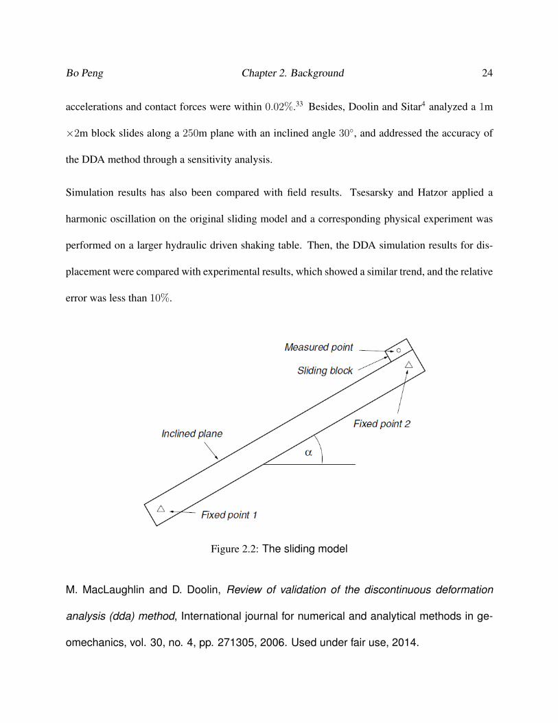
The sliding simulation model is shown in Figure 2.2 – a block under gravity slides along a fixed
inclined plane with an angle α and an interface friction angle φ. In this situation, the analytic
solution for the block’s displacement as a function of time is
d = 1/2at2 = 1/2(gSin(α)− gCos(α)Tan(φ))t2. (2.35)
So far, most validated simulation is based on the 2D-DDA model. Yeung27 studied 12 cases of a
sliding model with different combinations of slope angles and friction angles. Yueng also derived
an analytical solution for shear and normal contact forces. The difference between analytical re-
sults and simulation results was less than 0.5%. Maclauglin and Sitar28 proposed a ’gravity turn
on routine to reduce effects of a sudden loading in the initial time step. There are some other
validation models: a block decelerates along an incline with an initial velocity, with a maximum
error of 2%;29 a block with an initial speed stops due to the friction on a horizontal plane, with
error less than 0.1%;30 a block accelerates along a steep slope first and then transfers to a shallower
slope decelerating to a stop, and the DDA predicted maximum distance is 5% different from ana-
lytical solutions29, 31, 32 ; a block slides along an incline with friction and cohesion, where error on
Bo Peng Chapter 2. Background 24
accelerations and contact forces were within 0.02%.33 Besides, Doolin and Sitar4 analyzed a 1m
×2m block slides along a 250m plane with an inclined angle 30◦, and addressed the accuracy of
the DDA method through a sensitivity analysis.
Simulation results has also been compared with field results. Tsesarsky and Hatzor applied a
harmonic oscillation on the original sliding model and a corresponding physical experiment was
performed on a larger hydraulic driven shaking table. Then, the DDA simulation results for dis-
placement were compared with experimental results, which showed a similar trend, and the relative
error was less than 10%.
Figure 2.2: The sliding model
M. MacLaughlin and D. Doolin, Review of validation of the discontinuous deformation
analysis (dda) method, International journal for numerical and analytical methods in ge-
omechanics, vol. 30, no. 4, pp. 271305, 2006. Used under fair use, 2014.
Bo Peng Chapter 2. Background 25
With great effort from many researchers, the 2D-DDA has been well developed and verified. How-
ever, two dimensional models are restricted by assuming plane-strain or plane-stress conditions.
After Shi proposed a three-dimensional DDA (3D-DDA), a limited number of research work has
been done in this new area; this might be because of the very complex contact conditions for ar-
bitrary shaped blocks. Haztor and Bakun-Mazor3 reviewed current 3D-DDA results, and provided
a validation for a sliding block under a Sine horizontal acceleration using the 3D-DDA method.
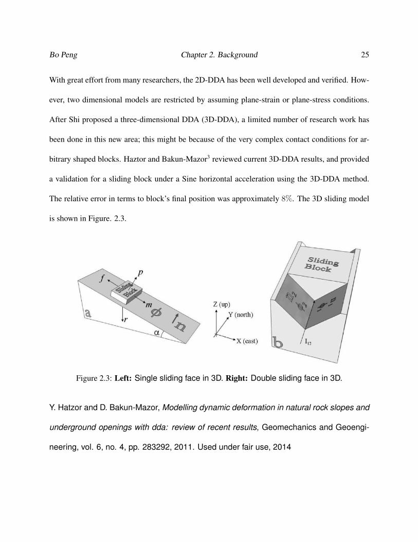
The relative error in terms to block’s final position was approximately 8%. The 3D sliding model
is shown in Figure. 2.3.
Figure 2.3: Left: Single sliding face in 3D. Right: Double sliding face in 3D.
Y. Hatzor and D. Bakun-Mazor, Modelling dynamic deformation in natural rock slopes and
underground openings with dda: review of recent results, Geomechanics and Geoengi-
neering, vol. 6, no. 4, pp. 283292, 2011. Used under fair use, 2014
Bo Peng Chapter 2. Background 26
2.3.2 Energy Dissipation Model
An impacting model is a typical model to test energy dissipation, and it was studied by Shyu15
through two 2D-DDA simulations: collision between two identical rods and collision between
two spheres moving towards each other in opposite directions. The displacement of each object,
the velocities of each object and the stress at contact points were recorded and compared with
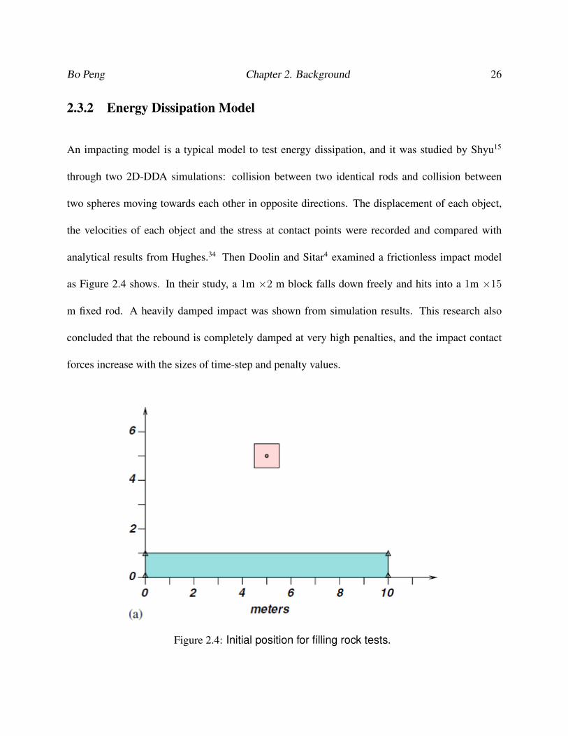
analytical results from Hughes.34 Then Doolin and Sitar4 examined a frictionless impact model
as Figure 2.4 shows. In their study, a 1m ×2 m block falls down freely and hits into a 1m ×15
m fixed rod. A heavily damped impact was shown from simulation results. This research also
concluded that the rebound is completely damped at very high penalties, and the impact contact
forces increase with the sizes of time-step and penalty values.
Figure 2.4: Initial position for filling rock tests.
Bo Peng Chapter 2. Background 27
D. M. Doolin and N. Sitar, Displacement accuracy of discontinuous deformation analysis
method applied to sliding block, Journal of engineering mechanics, vol. 128, no. 11, pp.
11581168, 2002. Used under fair use, 2014.
Energy dissipation has also been studied in time integration scheme analysis. Doolin and Sitar21 did
a comprehensive analysis on time integration for the 2D-DDA, which included a stability analysis
and an accuracy analysis for the DDA model. The time scheme applied in DDA (”right Riemann”)
has advantages of being unconditionally stable and ensure system energy dissipation, but it is
implicit and requires expensive iterations to solve. Jiang et al20 provided an exploration of energy
dissipation and convergence criterion for the DDA. Time-step sizes from 0.001s to 0.008s were
used to analyze energy dissipation. For convergence criteria, displacement, kinetic energy and
unbalanced force from the DDA solution were used for measurements. However, in this research,
they only explored the situation that acceleration remains constant during one time-step.
2.4 Challenges
Previous research has exhibited an obvious defect in the DDA: energy dissipation. According to
the energy conservation principle, there should be no energy loss in the completely elastic collision.
However, loss in energy openly appears in DDA simulations, especially when movement direction
changes suddenly. This energy dissipation occurs in the form of velocity and amplitude attenuation
even under undamped conditions. In order to overcome this shortcoming, we apply a new time
integration scheme to the DDA method: the Newmark method. The improved DDA method will
Bo Peng Chapter 2. Background 28
be testified through a sliding model and an impacting model. Besides, from previous work, we
can see that most of DDA work still remains in the 2D level. However, 3D models are important
for accuracy of simulations, because the unbalanced bounce and rotation resulting from energy
damping in 3D simulation are more obvious than that in 2D. Therefore, 3D-DDA simulations are
used in this thesis to simulate block sliding and bouncing.
Chapter 3
Newmark Method in 3D-DDA
In this chapter, we will first introduce the classic Newmark method,35 and then the applications of
the classic Newmark method to the DDA . Also, a new integrated Newmark method are illustrated.
3.1 Newmark Method
The Newmark method is a time-integration method, which shows the relationships between dis-
placement, velocity and acceleration. In each time-step of DDA simulation, the time integration
method updates the displacement, velocity and acceleration for every block based on the infor-
mation of previous time step. Since velocity and acceleration play key roles in forming stiffness
matrix in the linear equilibrium equation as mentioned in section 2.2.3, the time-integration method
can influence the accuracy of DDA simulation greatly.
29
Bo Peng Chapter 3. Newmark Method in 3D-DDA 30
Before the illustration of Newmark method in DDA, we will first clarify two set of symbols denot-
ing movement information.
• {u}n describes the accumulated displacement in general case, which denotes the accumu-
lated displacement at the end of current time-step. ˙{u}n represents the velocity and ¨{u}n
represents the acceleration.
• {D(t)}n = {Di} is the solution of the DDA linear equilibrium equation, and it describes
the displacement within current time-step. But ∂{D(t)}n∂t
, ∂2{D(t)}n∂t2
are still the velocity and
acceleration respectively: ∂{D(t)}n∂t
= ˙{u}n, ∂2{D(t)}n∂t2
= ¨{u}n.
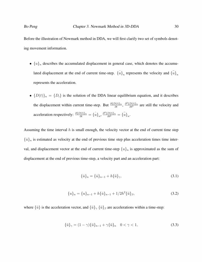
Assuming the time interval h is small enough, the velocity vector at the end of current time step
{u}n is estimated as velocity at the end of previous time step plus acceleration times time inter-
val, and displacement vector at the end of current time-step {u}n is approximated as the sum of
displacement at the end of previous time-step, a velocity part and an acceleration part:
{u}n = {u}n−1 + h{u}γ, (3.1)
{u}n = {u}n−1 + h{u}n−1 + 1/2h2{u}β, (3.2)
where {u} is the acceleration vector, and {u}γ {u}β are accelerations within a time-step:
{u}γ = (1− γ){u}n−1 + γ{u}n 0 < γ < 1, (3.3)
Bo Peng Chapter 3. Newmark Method in 3D-DDA 31
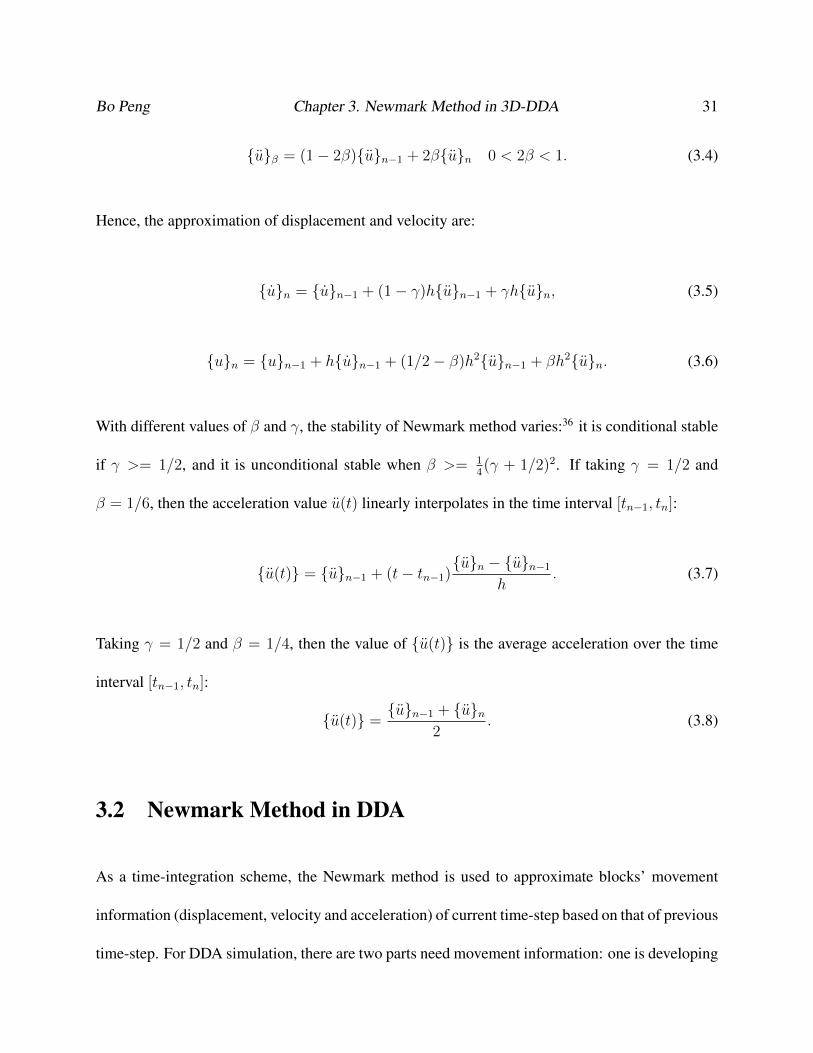
{u}β = (1− 2β){u}n−1 + 2β{u}n 0 < 2β < 1. (3.4)
Hence, the approximation of displacement and velocity are:
{u}n = {u}n−1 + (1− γ)h{u}n−1 + γh{u}n, (3.5)
{u}n = {u}n−1 + h{u}n−1 + (1/2− β)h2{u}n−1 + βh2{u}n. (3.6)
With different values of β and γ, the stability of Newmark method varies:36 it is conditional stable
if γ >= 1/2, and it is unconditional stable when β >= 14(γ + 1/2)2. If taking γ = 1/2 and
β = 1/6, then the acceleration value u(t) linearly interpolates in the time interval [tn−1, tn]:
{u(t)} = {u}n−1 + (t− tn−1){u}n − {u}n−1
h. (3.7)
Taking γ = 1/2 and β = 1/4, then the value of {u(t)} is the average acceleration over the time
interval [tn−1, tn]:
{u(t)} ={u}n−1 + {u}n
2. (3.8)
3.2 Newmark Method in DDA
As a time-integration scheme, the Newmark method is used to approximate blocks’ movement
information (displacement, velocity and acceleration) of current time-step based on that of previous
time-step. For DDA simulation, there are two parts need movement information: one is developing
Bo Peng Chapter 3. Newmark Method in 3D-DDA 32
submatrix of inertia force, another one is updating movement’s information at the end of each time-
step.
To develop the submatrix of inertia force for a block, (u(t), v(t), w(t)) are used to denote the
displacements at any point (x, y, z) in the time t. Then the inertia force per unit volume is given
by a product of weight density and acceleration:
fx
fy
fz
= −M
∂2u(t)∂t2
∂2v(t)∂t2
∂2w(t)∂t2
, (3.9)
Then the potential energy from the inertia force of the ith block can be denoted as an integration
of product of displacement and inertia force over volume:
Πi = −∫ ∫ ∫
(u v w)
fx
fy
fz
dx dy dz =
∫ ∫ ∫M{Di}T [Ti]
T [Ti]∂2{D(t)}
∂t2dx dy dz.
(3.10)
Take {D(t)}n−1 to denote the DDA displacement in the previous time step, {D(t)}n to denote the
displacement increment in the current time step, h to denote the time interval. Then applying the
Newmark method:
∂2{D(t)}n∂t2
=1
h2β{D(t)}n −
1
hβ
∂{D(t)}n−1∂t
− (1/2− β)
β
∂2{D(t)}n−1∂t2
, (3.11)
Bo Peng Chapter 3. Newmark Method in 3D-DDA 33
∂{D(t)}n∂t
=∂{D(t)}n−1
∂t+ (1− γ)h
∂2{D(t)}n−1∂t2
+ γh∂2{D(t)}n
∂t2. (3.12)
Replace the acceleration in the energy equation with Newmark acceleration, Eq. (3.10) can be
rewritten as:
Πi = {Di}T∫ ∫ ∫
[Ti]T [Ti]dx dy dz(
[M ]
h2β{D(t)}n−
[M ]
hβ
∂{D(t)}n−1∂t
−(1/2− β)[M ]
β
∂2{D(t)}n−1∂t2
).
(3.13)
As {D(t)}n = {Di}, minimizing the energy equation Eq. (3.13) with respect to {Di}T , we have
the stiffness submatrix and force sub-vector resulting from inertial force as:
(
∫ ∫ ∫[Ti]
T [Ti]dx dy dz)A→ [Kii],
(
∫ ∫ ∫[Ti]
T [Ti]dx dy dz)B → {Fi},(3.14)
where
A =[M ]
h2β,
B = ([M ]
hβ
∂{D(t)}n−1∂t
+(1/2− β)[M ]
β
∂2{D(t)}n−1∂t2
).
(3.15)
With Eq. (3.14)and Eq. (3.15), the Newmark method has been applied in the DDA method to
acquire the submatrix of inertia force.
Bo Peng Chapter 3. Newmark Method in 3D-DDA 34
3.3 The Energy Balance of the Newmark Method in DDA
The following part will prove the energy balance of the Newmark method in DDA method. Simpli-
fying the DDA model as a particle without regarding the stress and strain, then only point loading
and inertial force is considerate:
{Dn} = (h∂{D(t)}n−1
∂t+ h2(1/2− β)
∂2{D(t)}n−1∂t2
) + h2β∂2{D(t)}n
∂t2[M ]. (3.16)
For the traditional Newmark method, Krenk37 has proved its balance in energy. He denotes the
energy change in one time-step as:
(1/2 ˙{u}T
[M ] ˙{u}+ 1/2{u}T [K]{u})nn−1. (3.17)
After combing Eq. (3.17) with Newmark method Eq. (3.1), (3.2), then a reformulation of energy
change in one time-step is obtained as
(1/2 ˙{u}T
[M ] ˙{u}+ 1/2{u}T ([K] + (β − 1/2γ)h[K][M ]−1[K]){u})nn−1
= −(γ − 1/2){D}T ([K] + (β − 1/2γ)h[K][M ]−1[K]){u}){D},(3.18)
where the the original stiffness matrix can be replaced as an equivalent stiffness matrix: [K]eq =
[K] + (β − 1/2γ)h[K][M ]−1[K]). Note that if we take β = 1/4 in Eq. (3.16), then the solution
of DDA would be the same as the Newmark method taking β = 1/4, γ = 1/2, where Eq. (3.18)
suggests no energy dissipation.
Bo Peng Chapter 3. Newmark Method in 3D-DDA 35
3.4 The Integrated Newmark Method in DDA
Besides the classic Newamrk method, an integrated Newmark method is developed and applied to
the DDA method. Unlike the classic Newmark method, velocity and acceleration information are
not required for the integrated Newmark method when the linear equilibrium equation is developed.
The general kinetic function is:
[M ]{u}+ [C]{u}+ [K]{u} = {P}, (3.19)
where {u} is the accumulated displacement, [M] is the mass matrix, [C] is the damping matrix, [K]
is the stiffness matrix without considering the inertia force and {P} is the loading matrix without
inertia force. In order to convert the unknown variable {un} to displacement at each time step
{Dn}, considering the following four equations of four time-step under undamped situation:
[M ] ¨{u}n + [K]{u}n = {P}n, (3.20)
[M ] ¨{u}n−1 + [K]{u}n−1 = {P}n−1, (3.21)
[M ] ¨{u}n−2 + [K]{u}n−2 = {P}n−2, (3.22)
[M ] ¨{u}n−3 + [K]{u}n−3 = {P}n−3. (3.23)
Bo Peng Chapter 3. Newmark Method in 3D-DDA 36
After reorganizing equations as (Eq. (3.21)+Eq. (3.20))-(Eq. (3.22)+Eq. (3.23)), we have :
[M ][( ¨{u}n + ¨{u}n−1)− ( ¨{u}n−2 + ¨{u}n−3)] + [K][{u}n + {u}n−1 − {u}n−2 − {u}n−3]
= {P}n + {P}n−1 − {P}n−2 − {P}n−3.
(3.24)
As taking the newmark method is unconditional stable when γ = 1/2 and β = 1/4,36 we formulate
the Newmark method as:
˙{u}n = ˙{u}n−1 + 1/2h( ¨{u}n−1 + ¨{u}n), (3.25)
{u}n = {u}n−1 + h ˙{u}n−1 + 1/4h2( ¨{u}n−1 + ¨{u}n). (3.26)
Then, after Eq. (3.25) and Eq. (3.26) are combined, we have:
¨{u}n + ¨{u}n−1 =4
h2({u}n − {u}n−1) +
4
h˙{u}n−1. (3.27)
We can also obtain a reorganization, 2×Eq. (3.26) - Eq. (3.25), as:
{u}n − {u}n−1h
=˙{u}n + ˙{u}n−1
2. (3.28)
With Eq. (3.27) and Eq. (3.28), we can reformulate Eq. (3.24). The part of mass matrix [M ] in
Bo Peng Chapter 3. Newmark Method in 3D-DDA 37
Eq. (3.24) can be rewritten as:
[M ][( ¨{u}n + ¨{u}n−1)− ( ¨{u}n−2 + ¨{u}n−3)]
= [M ]{ 4
h2({D}n − {D}n−2)−
4
h( ˙{u}n−1 − ˙{u}n−3)}
= [M ]{ 4
h2({D}n − {D}n−2)−
4
h[( ˙{u}n−1 + ˙{u}n−1)− ( ˙{u}n−1 + ˙{u}n−3)]}
= [M ]{ 4
h2({D}n − 2{D}n−1 + {D}n−2)},
(3.29)
where:
{D}n = {u}n − {u}n−1,
{D}n−1 = {u}n−1 − {u}n−2,
{D}n−2 = {u}n−2 − {u}n−3.
(3.30)
The part of stiffness matrix [K] in Eq. (3.24) can also be rewritten as:
[K][{u}n + {u}n−1 − {u}n−2 − {u}n−3]
=[K][({u}n − {u}n−2) + ({u}n−1 − {u}n−3)]
=[K][({D}n + {D}n−1) + ({D}n−1 + {D}n−2)].
(3.31)
Finally, substituting Eq. (3.29) and Eq. (3.31) into Eq. (3.24), the equation of displacement in
Bo Peng Chapter 3. Newmark Method in 3D-DDA 38
each time-step can be formulated as:
[M ]{ 4
h2({D}n − 2{D}n−1 + {D}n−2)}+ [K][({D}n + {D}n−1) + ({D}n−1 + {D}n−2)]
= {P}n + {P}n−1 − {P}n−2 − {P}n−3.
(3.32)
As {D}n is the unknown variable, we reformulate Eq. (3.32) as:
[M ]4
h2{D}n + [K]{D}n
=[M ](4
h2(2{D}n−1 − {D}n−2)− [K](2× {D}n−1 + {D}n−2)
+ {P}n + {P}n−1 − {P}n−2 − {P}n−3.
(3.33)
Therefore, the submatrix of inertia force – stiffness submatrix and force subvector resulting from
inertia force – are:
[M ]4
h2→ [Kii],
[M ](4
h2(2{D}n−1 − {D}n−2)→ [Fi].
(3.34)
Also, the following part are required to be added to force vector in the global equation:
−[K](2× {D}n−1 + {D}n−2) + {P}n−1 − {P}n−2 − {P}n−3 → [Fi]. (3.35)
At this point, the Eq. (3.34) and Eq. (3.35) contend all the inertial force information that linear
equilibrium equation requires.
Chapter 4
Implement Details
So far, there is no sophisticated open source 3D-DDA code for simulating irregular shaped blocks.
Thanks to Professor Peng from China water and hydra resource institute, who contributed his
private 3D-DDA code, our experiment can be conducted based on it. The 3D-DDA code is an
extensible code developed in FORTRAN, and it is focused on implement of 3D-DDA Algorithm.
Because of the difficulty in 3D DDA simulation, this code is one of the few codes that able to
simulate the entire process of 3D block movements. But there are several challenges in revising
this code. The main problem is that the structure of this code is not well organized – its first version
was developed twenty years ago, and the optimization for this code are based on the first version’s
structure. Therefore, this code is not object-oriented, the entire code is just in one file.
39
Bo Peng Chapter 4. Implement Details 40
4.1 Structure of the DDA Code
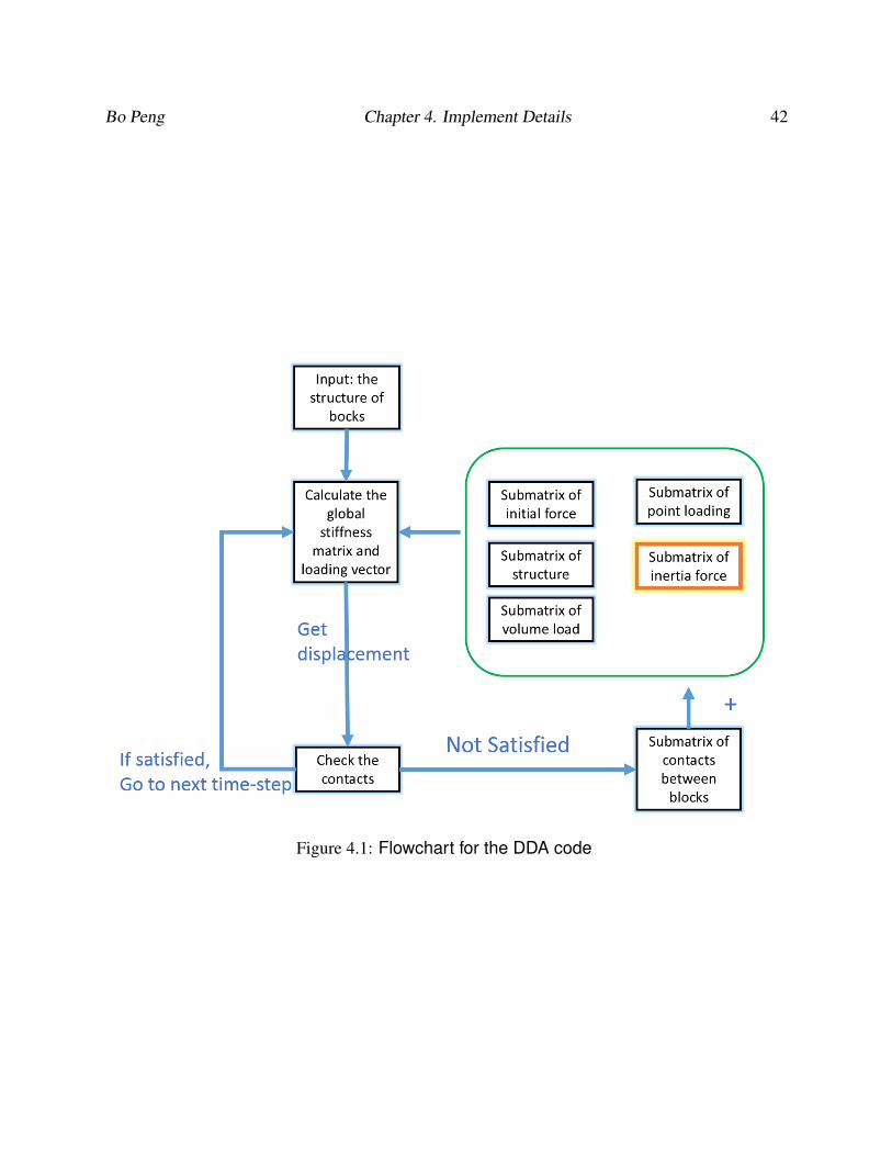
Because of the confusion of the code’s structure, it is necessary to understand the mechanism of
entire code. The Figure. 4.1 shows the a big picture of the DDA algorithm, including inputting
the block structure information, generating the stiffness matrix, solving the equation and checking
the contacts information. We will illustrate the structure of the DDA code through the following
functions:
• READ_PXC() is a function to read input files. There are two input files: Good.txt and
info.txt. The block structure information is stored in Good.txt , which includes the
surface number in each block, the point label in each surface, point coordinates, and equation
parameters for each surface. Other parameters are stored in the file Good.txt , including
Poisson ratio, Young’s modulus, gravity, etc.
• STIFF() is a function to determine the global stiffness matrix and right-side loading vector
in the linear equilibrium equation resulting from point load, volume load, initial stress, block
interactions. The theoretical details has been presented in section 2.2. The results are stored
in a 6n× (6n+ 1) matrix called ff(), where n is the number of unfixed blocks. In ff(),
the first 6n × 6n matrix stores the stiffness matrix information, and the last column is the
right-side loading vector.
• GXSTIFF() obtains the information of the submatrix of inertia force, and then adds it to
the global matrix ff().
Bo Peng Chapter 4. Implement Details 41
• SOLVER_PCG_zgx() applies preconditioned conjugate gradient (PCG) method to solve
the linear equilibrium equation, and the solution are the displacement and rotation of unfixed
blocks, which store in a 6n vector called ee(). However, in case of bad convergence rate
for PCG, a SOLUT3 () function employing the classic Gaussian elimination method will
be applied to resolve the linear equilibrium equation.
• NEWLOCATION() MACLENG() MAXMIN() MAXMINPLANE() check the contacts in-
formation when new location of unfixed blocks has been solved from the linear equilibrium
equation. If the new location of blocks are not satisfied with the contacting law, such as
tensile force existing between blocks, then the stiffness matrix need to be redeveloped. A
variable called MCBH records the friction status; if the friction status changes, the stiffness
matrix will also be recalculated. The stiffness matrix maybe regenerated several times, and
the simulation would not step into the next time-step unless the solution of equilibrium equa-
tion satisfies all contacting laws.
• DT() is a function to export the blocks’ coordinate information and to update other infor-
mation, such as velocity and acceleration. It will only be called once at the end of every
time-step.
There are also quit a large number of functions to handle the details, such as T_DELT() to adjust
time-step size, MIDJL to record error information.
Bo Peng Chapter 4. Implement Details 42
Figure 4.1: Flowchart for the DDA code
Bo Peng Chapter 4. Implement Details 43
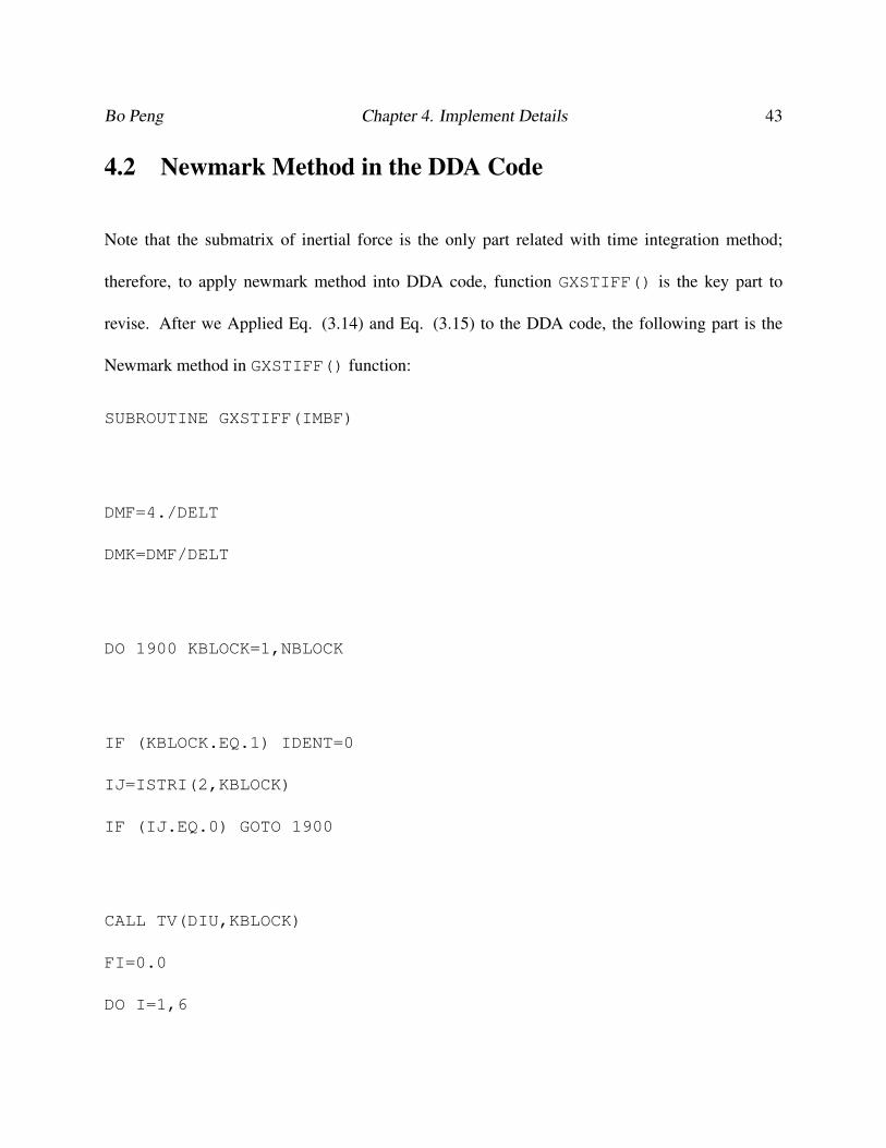
4.2 Newmark Method in the DDA Code
Note that the submatrix of inertial force is the only part related with time integration method;
therefore, to apply newmark method into DDA code, function GXSTIFF() is the key part to
revise. After we Applied Eq. (3.14) and Eq. (3.15) to the DDA code, the following part is the
Newmark method in GXSTIFF() function:
SUBROUTINE GXSTIFF(IMBF)
DMF=4./DELT
DMK=DMF/DELT
DO 1900 KBLOCK=1,NBLOCK
IF (KBLOCK.EQ.1) IDENT=0
IJ=ISTRI(2,KBLOCK)
IF (IJ.EQ.0) GOTO 1900
CALL TV(DIU,KBLOCK)
FI=0.0
DO I=1,6
Bo Peng Chapter 4. Implement Details 44
DO J=1,6
FI(I)=FI(I)+FFS(I,J,KBLOCK)*DIU(J)*GAMA
ENDDO
ENDDO
DO I=1,6
DO J=1,6
KII(I,J)=FFS(I,J,KBLOCK)*DMK*GAMA
ENDDO
ENDDO
CALL DRZKII(KBLOC,KII,FI)
1900 CONTINUE
RETURN
END
The function GXSTIFF() is the last part to form the global stiffness matrix, and it runs after
STIFF(). The return value of TV() is a vector DIU(6), storing the value of (4∂[D(t)n−1]∂t
−
2∂2[D(t)n−1]
∂t2) of the KBLOCK’s object. FFS() is the mass matrix, which is [M ] in Eq. (3.14) and
Eq. (3.15). After the submatrix of inertial force has been acquired, a function DRZKII () will
Bo Peng Chapter 4. Implement Details 45
map the local stiffness matrix into the global matrix.
Besides the GXSTIFF(), the velocity and acceleration should be updated at the end of each time-
step:
ACCEL()=4./DELT/DELT*DIU()-4./DELT*VEL_1()-ACCEL_1()
VEL()=VEL_1()+0.5*DELT*(ACCEL_1()+ACCEL())
4.3 Implement of the Integrated Newmark Method in the DDA
Code
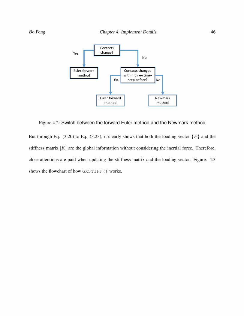
Apply the integrated Newmark method into DDA code is more complicated. Because the loading
vector of current time-step relies on the loading vectors in previous time-step, and the equation is
deducted based on the assumption that the mass matrix [M ] and stiffness matrix [K] remain the
same in recent four time-steps. As a result, the Newmark method can not be applied during the
whole process. As [M ] is only related with the structure of block, [M ] does not change during
the entire simulation process. However, [K] changes whenever the contacts vary. Therefore, once
contact status changes, the forward Euler method will be applied. After contacts status keep the
same for three time-steps, Newmark method will be applied again. This process is shown in Figure
4.2.
The function GXSTIFF(), which is used for obtaining the submatrix of inertial force, is the key
part to apply the integrated Newmark method. This part is based on the Eq. (3.34) and Eq. (3.35).
Bo Peng Chapter 4. Implement Details 46
Figure 4.2: Switch between the forward Euler method and the Newmark method
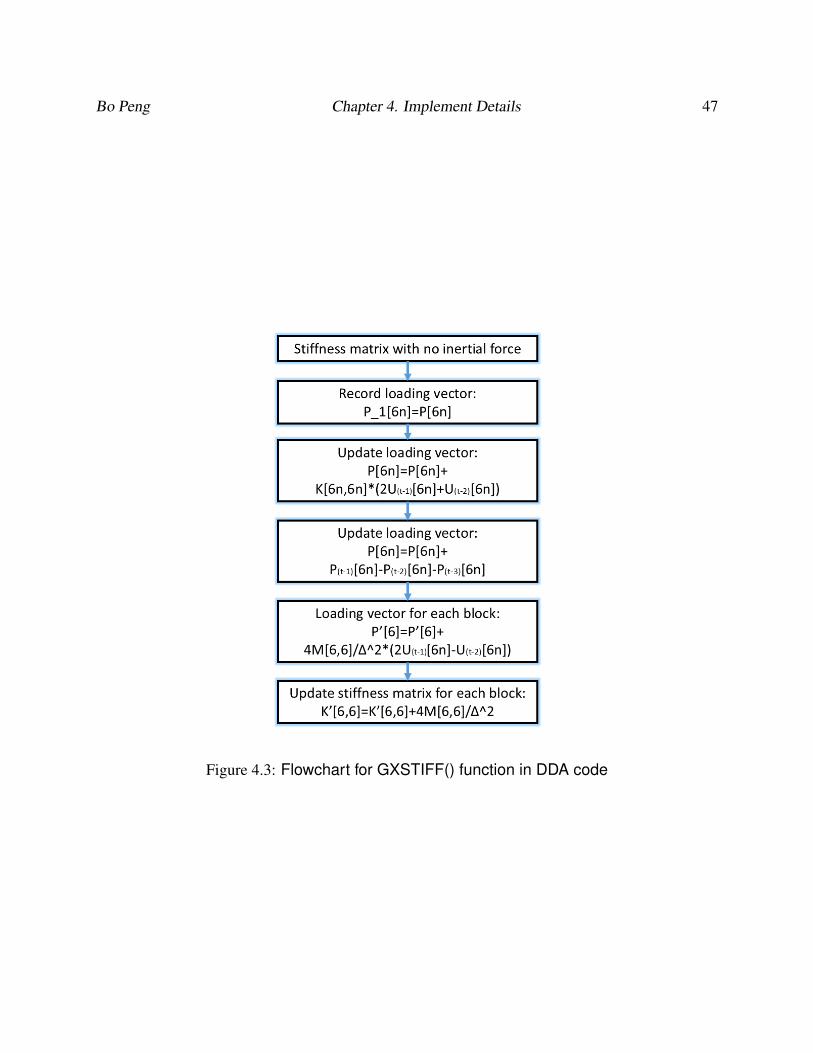
But through Eq. (3.20) to Eq. (3.23), it clearly shows that both the loading vector {P} and the
stiffness matrix [K] are the global information without considering the inertial force. Therefore,
close attentions are paid when updating the stiffness matrix and the loading vector. Figure. 4.3
shows the flowchart of how GXSTIFF() works.
Bo Peng Chapter 4. Implement Details 47
Figure 4.3: Flowchart for GXSTIFF() function in DDA code
Chapter 5
Results and Analysis
In this chapter, we will report the simulation results for two DDA models. The first model is
a sliding model, which composed of a fixed incline and a small block. The second model is
an impacting model, in which a small block impacts a fixed horizontal surface. As the DDA is
designed for solving discrete systems, contacting between objects can be regarded as the most
important part in simulation. A contact is composed of a tangential direction contact and a normal
direction contact. A sliding model is a great example for simulating tangential contacts and an
impacting model is for normal contacts. Therefore, both models are the very fundamental for
DDA verification. The general structures of these two models are illustrated, and the experiment
results will be shown.
To show the accuracy improvements by the Newmark method, the forward Euler method is used
for comparison. Before this study, the forward Euler method is the only time-integration scheme
48
Bo Peng Chapter 5. Results and Analysis 49
applied in the DDA simulation. It is a very stable method, while resulting in strong damping
effects at the same time.21 This damping effect becomes more obvious when a sudden change of
movement direction occurs.
The DDA code we use is offered by Professor Peng from China Institute of Water Resource and
Hydropower Research, and it is developed by Fortran. After models have been developed, the dis-
placement of the center of block is used to compare the accuracy of two different time integration
methods. So far, most research in DDA are restricted to two dimensional simulation, but in this
study both models are three dimensional models with six degree of freedoms – displacement in
x,y,z directions and rotation in x,y,z directions. The three dimensional results will be compared
with analytical solution, and the relative error will be measured.
5.1 Sliding Model
A sliding model represents a simplified model to simulate rocks sliding along structure surfaces,
as they share similar boundary conditions: the rock(block) slides in the direction of slope with no
restriction in other direction.
The points of this experiment are: 1) to validate the 3D-DDA method through comparison between
analytically solution and simulation solution, 2) to compare the accuracy of the Newmark method
and the forward Euler method, 3) to explore the computational costs for these two time-integration
method.
Bo Peng Chapter 5. Results and Analysis 50
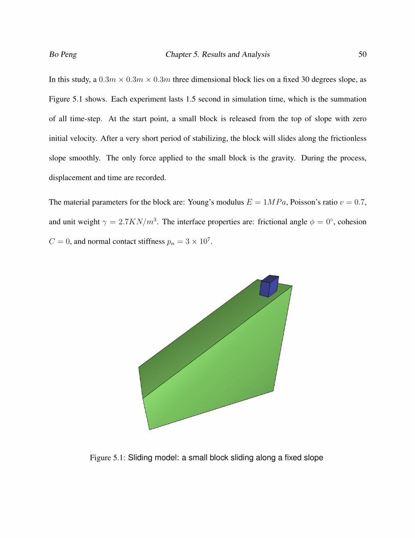
In this study, a 0.3m × 0.3m × 0.3m three dimensional block lies on a fixed 30 degrees slope, as
Figure 5.1 shows. Each experiment lasts 1.5 second in simulation time, which is the summation
of all time-step. At the start point, a small block is released from the top of slope with zero
initial velocity. After a very short period of stabilizing, the block will slides along the frictionless
slope smoothly. The only force applied to the small block is the gravity. During the process,
displacement and time are recorded.
The material parameters for the block are: Young’s modulus E = 1MPa, Poisson’s ratio v = 0.7,
and unit weight γ = 2.7KN/m3. The interface properties are: frictional angle φ = 0◦, cohesion
C = 0, and normal contact stiffness pn = 3× 10⁷.
Figure 5.1: Sliding model: a small block sliding along a fixed slope
Bo Peng Chapter 5. Results and Analysis 51
5.1.1 Accuracy Analysis
To validate the DDA method, a simulation of sliding model was conduct. For this simulation,
the time-step is fixed as 0.002s, and the trajectory of small block within a total 1.5s simulation
time were recorded. Figure 5.2 displays the results: a comparison between DDA solution using
the forward Euler time integration, DDA solution using the Newmark time integration and the
analytical solution. The picture shows that the displacement of DDA method using both time
integration schemes are very close to the analytical solution:
d =1
2g(sin(α)− cos(α)tan(φ))t2 (5.1)
where d is the displacement, α is the degree of slope, φ is the frictional angle which is zero here, t
is the accumulated time. To measure the accuracy of the forward Euler method and the Newmark
method, we define a relative error as:
Er = (Ds −Da)/Da (5.2)
where Er is the relative error, Ds is the simulated displacement and Da is the analytical displace-
ment. Figure 5.3 illustrates the relative error based on the same results of Figure. 5.2. It shows
that the beginning of DDA simulation is not very stable, and relative errors change quickly. That
is because the block adjusts itself to a stable condition when it contacts with the slope at the very
beginning. But after the block starts to slide steadily along the slope, the relative errors for both
Bo Peng Chapter 5. Results and Analysis 52
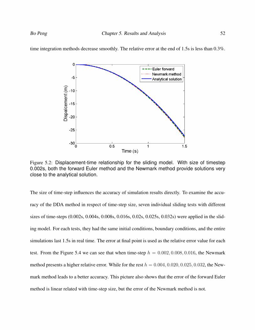
time integration methods decrease smoothly. The relative error at the end of 1.5s is less than 0.3%.
Figure 5.2: Displacement-time relationship for the sliding model. With size of timestep0.002s, both the forward Euler method and the Newmark method provide solutions veryclose to the analytical solution.
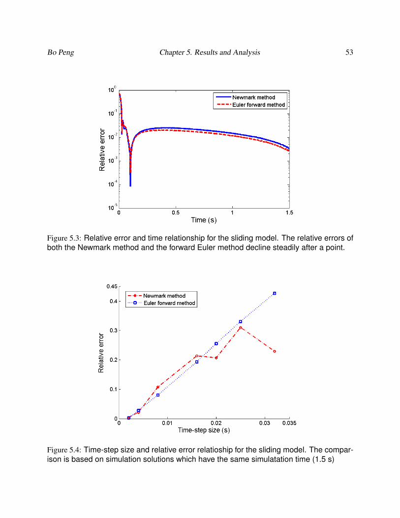
The size of time-step influences the accuracy of simulation results directly. To examine the accu-
racy of the DDA method in respect of time-step size, seven individual sliding tests with different
sizes of time-steps (0.002s, 0.004s, 0.008s, 0.016s, 0.02s, 0.025s, 0.032s) were applied in the slid-
ing model. For each tests, they had the same initial conditions, boundary conditions, and the entire
simulations last 1.5s in real time. The error at final point is used as the relative error value for each
test. From the Figure 5.4 we can see that when time-step h = 0.002, 0.008, 0.016, the Newmark
method presents a higher relative error. While for the rest h = 0.004, 0.020, 0.025, 0.032, the New-
mark method leads to a better accuracy. This picture also shows that the error of the forward Euler
method is linear related with time-step size, but the error of the Newmark method is not.
Bo Peng Chapter 5. Results and Analysis 53
Figure 5.3: Relative error and time relationship for the sliding model. The relative errors ofboth the Newmark method and the forward Euler method decline steadily after a point.
Figure 5.4: Time-step size and relative error relatioship for the sliding model. The compar-ison is based on simulation solutions which have the same simulatation time (1.5 s)
Bo Peng Chapter 5. Results and Analysis 54
5.1.2 Computational Time Comparison
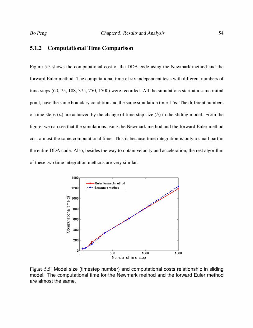
Figure 5.5 shows the computational cost of the DDA code using the Newmark method and the
forward Euler method. The computational time of six independent tests with different numbers of
time-steps (60, 75, 188, 375, 750, 1500) were recorded. All the simulations start at a same initial
point, have the same boundary condition and the same simulation time 1.5s. The different numbers
of time-steps (n) are achieved by the change of time-step size (h) in the sliding model. From the
figure, we can see that the simulations using the Newmark method and the forward Euler method
cost almost the same computational time. This is because time integration is only a small part in
the entire DDA code. Also, besides the way to obtain velocity and acceleration, the rest algorithm
of these two time integration methods are very similar.
Figure 5.5: Model size (timestep number) and computational costs relationship in slidingmodel. The computational time for the Newmark method and the forward Euler methodare almost the same.
Bo Peng Chapter 5. Results and Analysis 55
5.2 Impacting Model
Impacting model is composed of a fixed surface and a small block which can move freely. It is a
very important validation model for DDA simulation to test how normal contacts between blocks
work, and how they work under condition of trajectory direction changes rapidly. The impacting
process in simulation can be classified as two part: contacting and non-contacting parts. When
blocks contact with each other, they are connected by two artificial springs: a normal one and a
tangential one. When blocks are not contacting, they moves independently, and the only force the
small block took is the gravity.
As the direction of movements change during a relatively small time of contacting in the impacting
model, strong damping effects occur even in undamped cases when the forward Euler method is
applied. This is against the theoretical solution, because there is no energy dissipation shown in
the DDA equation. Being a challenge in the DDA simulation for a long time, the unreasonable
damping effects can be vanished by applying the Newmark method, and it will greatly increase the
accuracy of the DDA.
The points of this experiment are: 1) to demonstrate the significant accuracy improvements through
using the Newmark method, 2) to explore how the time-step size effects the accuracy of the forward
Euler method and the Newmark method.
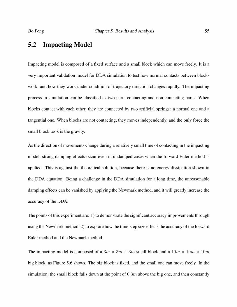
The impacting model is composed of a 3m × 3m × 3m small block and a 10m × 10m × 10m
big block, as Figure 5.6 shows. The big block is fixed, and the small one can move freely. In the
simulation, the small block falls down at the point of 0.3m above the big one, and then constantly
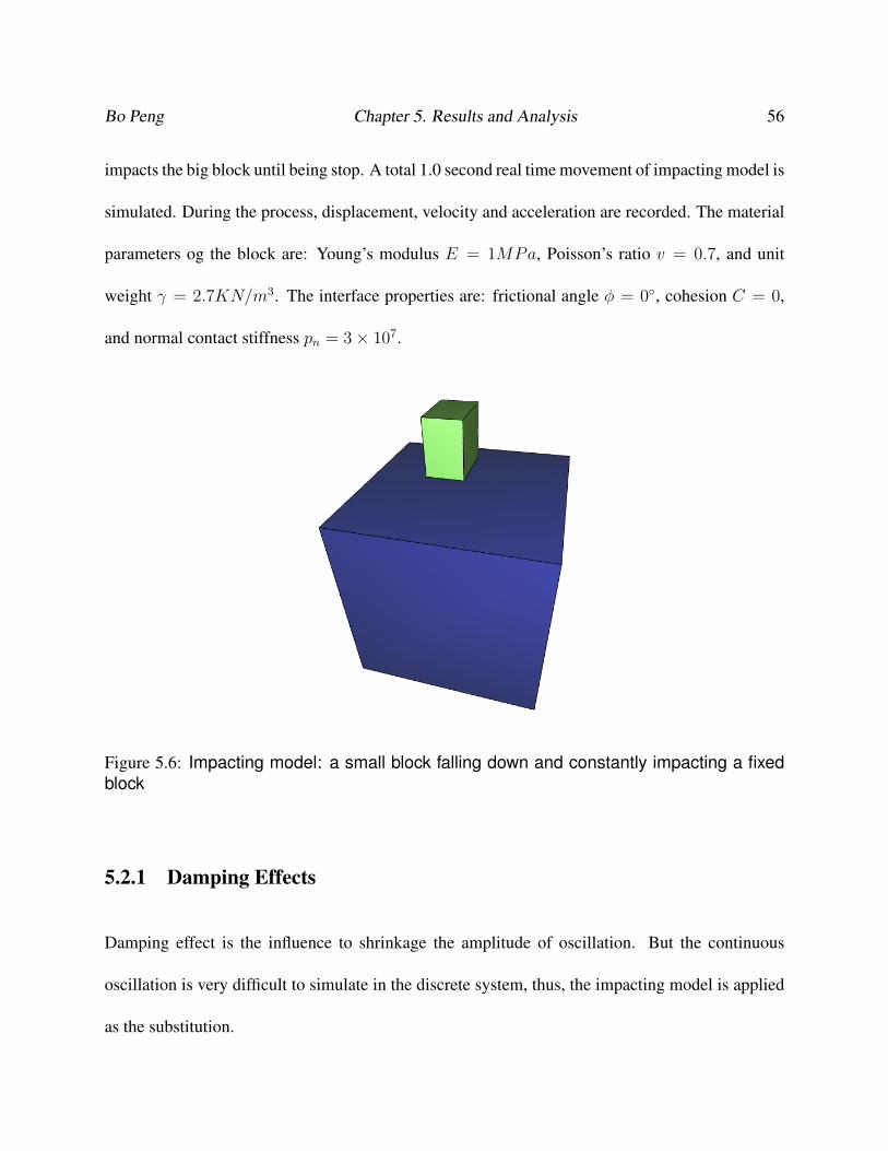
Bo Peng Chapter 5. Results and Analysis 56
impacts the big block until being stop. A total 1.0 second real time movement of impacting model is
simulated. During the process, displacement, velocity and acceleration are recorded. The material
parameters og the block are: Young’s modulus E = 1MPa, Poisson’s ratio v = 0.7, and unit
weight γ = 2.7KN/m3. The interface properties are: frictional angle φ = 0◦, cohesion C = 0,
and normal contact stiffness pn = 3× 10⁷.
Figure 5.6: Impacting model: a small block falling down and constantly impacting a fixedblock
5.2.1 Damping Effects
Damping effect is the influence to shrinkage the amplitude of oscillation. But the continuous
oscillation is very difficult to simulate in the discrete system, thus, the impacting model is applied
as the substitution.
Bo Peng Chapter 5. Results and Analysis 57
In this study, three time integration methods are going to be explored: the forward Euler method,
the classic Newmark method and the integrated Newmark method. The simulation results of dis-
placement, velocity and acceleration are compared with analytical results:
∆d = v × h+1
2× a× h2. (5.3)
This is the analytical solution for a one dimensional problem, and the object is idealized as a
particle. This situation is usually simulated by a Single-degree of freedom system in previous
research.20, 21 However, in the 3D-DDA simulation, we use a six degree of freedom model: the
small block will impact the fixed surface with its entire bottom plane, and it is possible to rotate or
move to any direction.
In this experiment, the bottom plane of the small block is parallel to the fixed ground surface, and
no friction is applied in contacts. As the small block shows barely any offset in Y,Z direction,
only the vertical trajectory of its mass center is recorded for comparison analysis. Figures 5.7-5.9
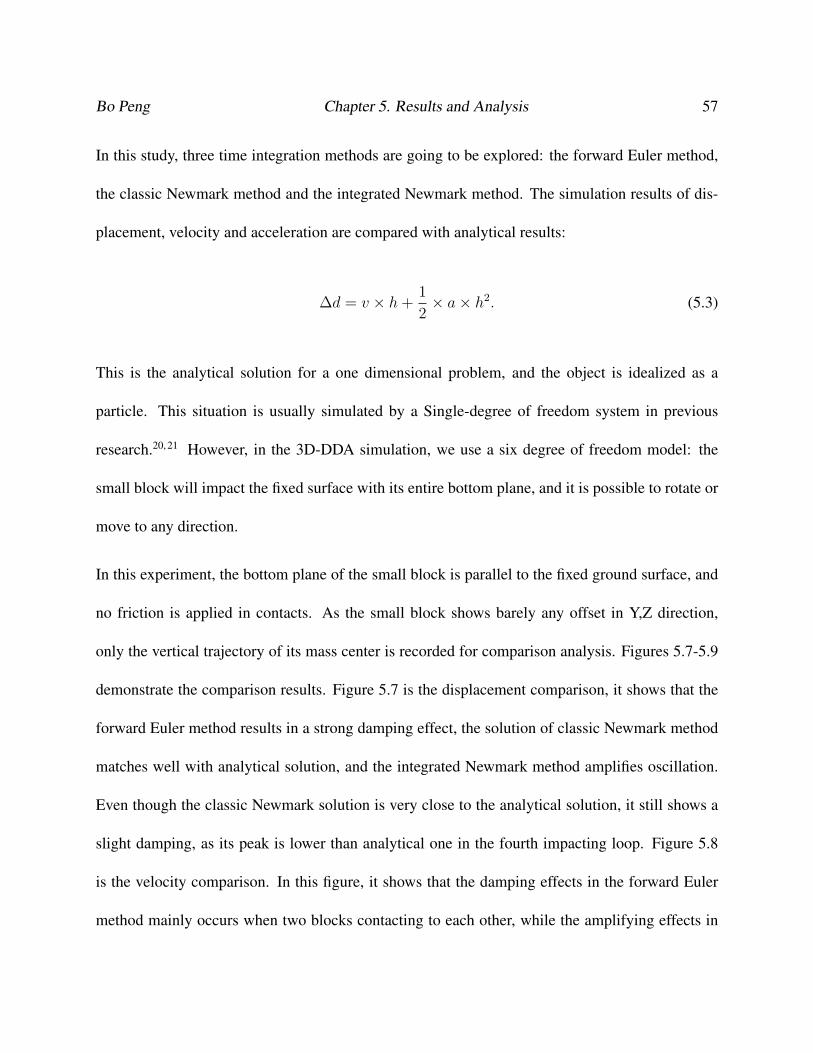
demonstrate the comparison results. Figure 5.7 is the displacement comparison, it shows that the
forward Euler method results in a strong damping effect, the solution of classic Newmark method
matches well with analytical solution, and the integrated Newmark method amplifies oscillation.
Even though the classic Newmark solution is very close to the analytical solution, it still shows a
slight damping, as its peak is lower than analytical one in the fourth impacting loop. Figure 5.8
is the velocity comparison. In this figure, it shows that the damping effects in the forward Euler
method mainly occurs when two blocks contacting to each other, while the amplifying effects in
Bo Peng Chapter 5. Results and Analysis 58
the integrated Newmark method imbedded in the entire process – both when two blocks contact
and separate. We believe this is an inner defect of the integrated method, but the reason is not
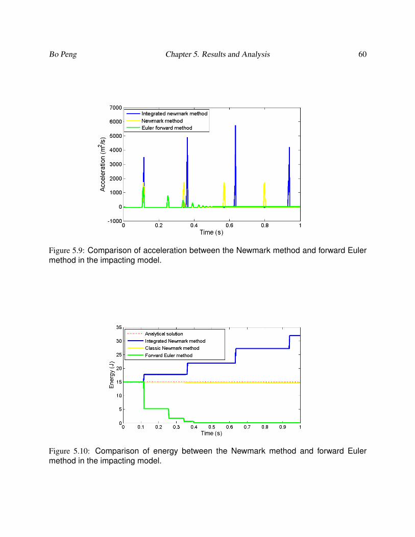
clear yet. Figure 5.9 shows the acceleration information: their peak values, which happen in
contacting, demonstrate how stable for the impacting process. Peaks in the forward Euler method
decrease linearly, those in the classic Newmark method keep the same in each loop, and that in the
integrated Newmark method have no stable trend.
Generally speaking, the integrated Newmark method does not show a good match with analytical
solution. But so far, we do not know the reason. It might be because of the defects in either
equation deduction or the code. Therefore, the rest analysis will not include Integrated Newmark
method.
Figure 5.10 shows the energy change in the impacting process, which verifies the energy conser-
vation of the Newmark method. It also shows a damping effect in forward Euler method and an
amplifying effect in the integrated Newmark method.
5.2.2 Time-step effects
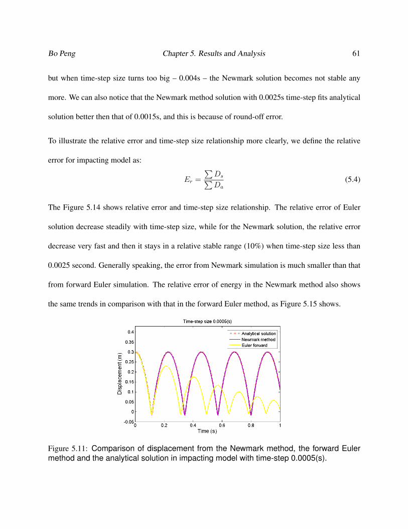
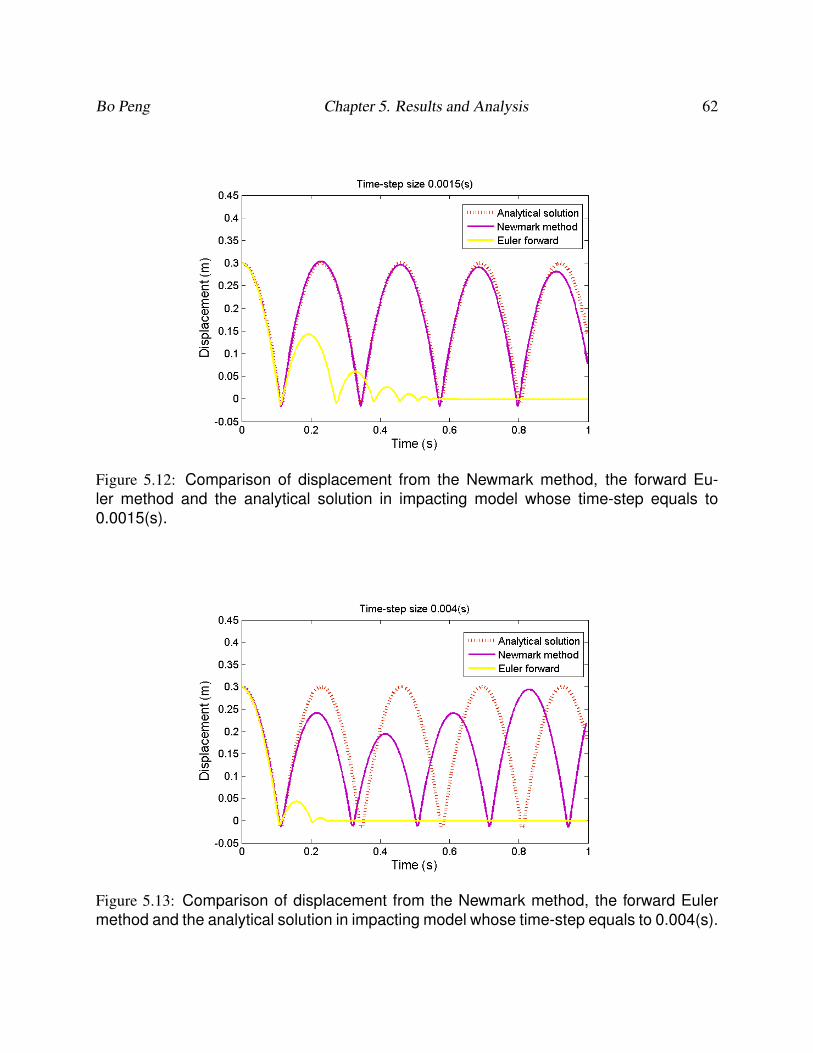
Time-step is closely related with the accuracy of a simulation. Figures 5.11-5.13 show the impact-
ing model simulation results when different time-step sizes (0.0005s, 0.0015s, 0.0025s, 0.004s) are
applied. From these four Figures, we can tell that damping effects from the forward Euler method
increasing with increment of time-step size. For the Newmark method, the solution matches with
analytical solution reasonable well when time-step size equals to 0.0005s, 0.0015s and 0.0025s,
Bo Peng Chapter 5. Results and Analysis 59
Figure 5.7: Comparison of displacement between the Newmark method, the forward Eulermethod and the analytical solution in the impacting model. With a time-step size 0.002(s),the forward Eular method shows strong damping effects; the classic Newmark methodillustrates a good match with analytical solution; and the integrated Newmark method hasan amplifed effects.
Figure 5.8: Comparison of velocity between the Newmark method, forward Euler methodand analytical solution in the impacting model.
Bo Peng Chapter 5. Results and Analysis 60
Figure 5.9: Comparison of acceleration between the Newmark method and forward Eulermethod in the impacting model.
Figure 5.10: Comparison of energy between the Newmark method and forward Eulermethod in the impacting model.
Bo Peng Chapter 5. Results and Analysis 61
but when time-step size turns too big – 0.004s – the Newmark solution becomes not stable any
more. We can also notice that the Newmark method solution with 0.0025s time-step fits analytical
solution better then that of 0.0015s, and this is because of round-off error.
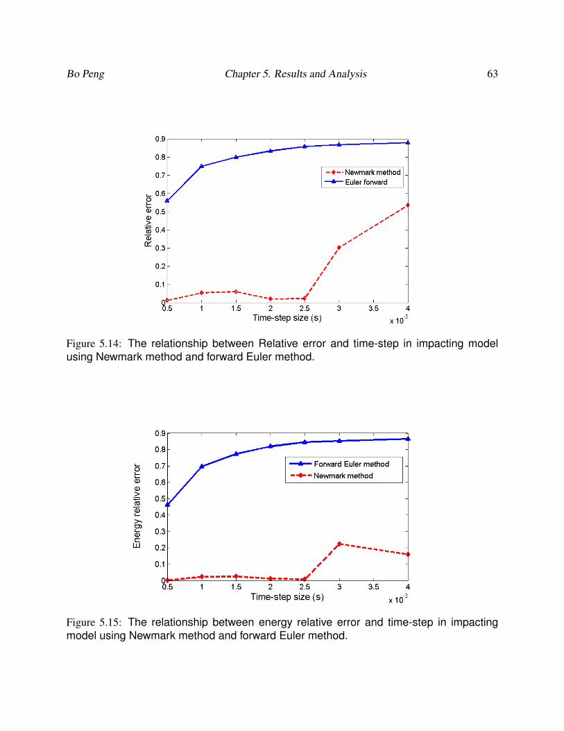
To illustrate the relative error and time-step size relationship more clearly, we define the relative
error for impacting model as:
Er =
∑Ds∑Da
(5.4)
The Figure 5.14 shows relative error and time-step size relationship. The relative error of Euler
solution decrease steadily with time-step size, while for the Newmark solution, the relative error
decrease very fast and then it stays in a relative stable range (10%) when time-step size less than
0.0025 second. Generally speaking, the error from Newmark simulation is much smaller than that
from forward Euler simulation. The relative error of energy in the Newmark method also shows
the same trends in comparison with that in the forward Euler method, as Figure 5.15 shows.
Figure 5.11: Comparison of displacement from the Newmark method, the forward Eulermethod and the analytical solution in impacting model with time-step 0.0005(s).
Bo Peng Chapter 5. Results and Analysis 62
Figure 5.12: Comparison of displacement from the Newmark method, the forward Eu-ler method and the analytical solution in impacting model whose time-step equals to0.0015(s).
Figure 5.13: Comparison of displacement from the Newmark method, the forward Eulermethod and the analytical solution in impacting model whose time-step equals to 0.004(s).
Bo Peng Chapter 5. Results and Analysis 63
Figure 5.14: The relationship between Relative error and time-step in impacting modelusing Newmark method and forward Euler method.
Figure 5.15: The relationship between energy relative error and time-step in impactingmodel using Newmark method and forward Euler method.
Bo Peng Chapter 5. Results and Analysis 64
5.3 Summary
The results analysis of the sliding model and the impacting model suggest that the classic Newmark
method significantly restricts the damping affects and improves the accuracy, while computational
costs remain in the same level. Considering the velocity is the first order derivative of displace-
ment and acceleration is the second order derivative, then the forward Euler method is a first order
approximation, and the Newmark method can be considered as a second order approximation. For
the impacting process, the change of moving direction results in a sudden change of much higher
value of acceleration than average acceleration, and in this situation the second order approxima-
tion is able to provide a much better solution than the first order one. For the sliding model, two
time-integration method have a similar accuracy as the acceleration keeps the same in the entire
process.
Chapter 6
Conclusion and Future Work
We investigated two time integration methods: the forward Euler method and the Newmark method
applied to the DDA. Prior to this work, only the forward Euler method was used as a time integra-
tion method in the DDA. The forward Euler method is a very stable method, but it leads to severe
damping effects in contacting simulation, which is against the corresponding theoretical solution.
The major contribution of this work is to derive the Newmark method and apply it to the DDA.
The Newmark method avoids the damping effects resulted from time integration simulation. Our
work also shows a complete three dimensional DDA simulation, which is rare so far as we know.
It has been an open question for some time whether the damping effect in DDA is an inner defect.
With the impacting model, we can see that the damping effects will shrinkage with time-step size,
which indicates that when the time-step is small enough, the error resulted from the damping effects
can be ignored. But that will cost a high computational time. On the other hand, the Newmark
65
Bo Peng Chapter 6. Conclusion and Future Work 66
method keeps the damping effect relatively low when time-step size is reasonable.
In this thesis, for theoretical part, we derived the formula and applied the Newmark method to the
DDA. We also developed an integrated Newmark method, in which no velocity and acceleration
were included when solving the linear equilibrium equation. But the integrated method is more
complicated in practice, and the simulation results show amplifying effects.
For the simulation part, two very basic and very widely used models are applied to test the forward
Euler method and the Newmark method. The first one is a sliding model, both the forward Euler
method and the Newmark method show a good match with analytical results. The second model
is an impacting model, in which the Newmark method shows a much better accuracy than the
forward Euler method, and there are barely damping effects.
In future work, more simulations under boarder range of situations are needed to understand how
the Newmark method in the DDA works. Also more work could be done to explore Newmark
parameters γ, β. We tried to use some different combination of γ, β, but because of the limite
of time, the data is not sufficient for meaningful conclusion can be drawn so far. We expect the
introduction of the Newmark method improves the accuracy of the DDA and be more widely used
in more complected simulations
Bibliography
[1] Y. Liu, Discrete element methods for asphalt concrete: development and application of user-
defined microstructural models and a viscoelastic micromechanical model. Michigan Tech-
nological University, 2011.
[2] M. MacLaughlin and D. Doolin, “Review of validation of the discontinuous deformation
analysis (dda) method,” International journal for numerical and analytical methods in ge-
omechanics, vol. 30, no. 4, pp. 271–305, 2006.
[3] Y. Hatzor and D. Bakun-Mazor, “Modelling dynamic deformation in natural rock slopes and
underground openings with dda: review of recent results,” Geomechanics and Geoengineer-
ing, vol. 6, no. 4, pp. 283–292, 2011.
[4] D. M. Doolin and N. Sitar, “Displacement accuracy of discontinuous deformation analy-
sis method applied to sliding block,” Journal of engineering mechanics, vol. 128, no. 11,
pp. 1158–1168, 2002.
[5] A. Hrennikoff, “Solution of problems of elasticity by the framework method,” Journal of
applied mechanics, vol. 8, no. 4, pp. 169–175, 1941.
67
Bibliography 68
[6] K. Feng, “Difference schemes for hamiltonian formalism and symplectic geometry,” Journal
of Computational Mathematics, vol. 4, no. 3, pp. 279–289, 1986.
[7] P. A. Cundall and O. D. Strack, “A discrete numerical model for granular assemblies,”
Geotechnique, vol. 29, no. 1, pp. 47–65, 1979.
[8] G.-h. Shi, Discontinuous deformation analysis: a new numerical model for the statics and
dynamics of block systems. PhD thesis, University of California, Berkeley, 1988.
[9] N. Shimizu, H. Kakihara, H. Terato, K. Nakagawa, et al., “A back analysis method for pre-
dicting deformational behavior of discontinuous rock mass,” in 2nd North American Rock
Mechanics Symposium, American Rock Mechanics Association, 1996.
[10] T.-C. Ke and J. Bray, “Modeling of particulate media using discontinuous deformation anal-
ysis,” Journal of engineering mechanics, vol. 121, no. 11, pp. 1234–1243, 1995.
[11] Y. Ohnishi, G. Chen, and S. Miki, “Recent development of dda in rock mechanics,” Proc.
ICADD, vol. 1, pp. 26–47, 1995.
[12] G.-h. Shi et al., “Three dimensional discontinuous deformation analyses,” in DC Rocks 2001
The 38th US Symposium on Rock Mechanics (USRMS), American Rock Mechanics Associa-
tion, 2001.
[13] T. Ke, “Improved modeling of rock bolting in dda,” in Proc., 9th Int. Conf. on Computer
Methods and Advances in Geomechanics, pp. 483–488, Balkema, Rotterdam, The Nether-
lands, 1997.
Bibliography 69
[14] M. Yeung, Q. Jiang, and N. Sun, “Validation of block theory and three-dimensional discon-
tinuous deformation analysis as wedge stability analysis methods,” International Journal of
Rock Mechanics and Mining Sciences, vol. 40, no. 2, pp. 265–275, 2003.
[15] K. Shyu, X. Wang, and C. Chang, “Dynamic behaviors in discontinuous elastic media using
dda,” in Proceedings of the Third International Conference on Analysis of Discontinuous
Deformation from Theory to Practice, pp. 243–252, 1999.
[16] X. Dong, A. Wu, and F. Ren, “A preliminary application of discontinuous deformation anal-
ysis (dda) to the three gorges project on yangtze river, china,” in Proceedings of the first
international forum on discontinuous deformation analysis (DDA) and simulations of dis-
continuous media, Berkeley, USA, pp. 310–317, 1996.
[17] H. K. Law and I. P. Lam, “Evaluation of seismic performance for tunnel retrofit project,”
Journal of geotechnical and geoenvironmental engineering, vol. 129, no. 7, pp. 575–589,
2003.
[18] Y. Hatzor et al., “Dynamic rock slope stability analysis at masada national monument using
block theory and dda,” Rock Mecganics for Industry, vol. 1, pp. 63–70, 1999.
[19] J. Kottenstette, “Dda analysis of the rcc modification for pueblo dam,” in Proceedings of
Third International Conference on Analysis of Discontinuous Deformation-From Theory To
Practice, Vail, Co, Jun, pp. 3–4, 1999.
Bibliography 70
[20] Q. Jiang, Y. Chen, C. Zhou, and M.-c. R. Yeung, “Kinetic energy dissipation and convergence
criterion of discontinuous deformations analysis (dda) for geotechnical engineering,” Rock
mechanics and rock engineering, vol. 46, no. 6, pp. 1443–1460, 2013.
[21] D. M. Doolin and N. Sitar, “Time integration in discontinuous deformation analysis,” Journal
of engineering mechanics, vol. 130, no. 3, pp. 249–258, 2004.
[22] M. Tsesarsky, Y. Hatzor, and N. Sitar, “Dynamic block displacement prediction–validation of
dda using analytical solutions and shaking table experiments,” in Stability of rock structures:
Proceedings of the Fifth International Conference of Analysis of Discontinuous Deformation.
Lisse: Balkema Publishers, pp. 195–203, 2002.
[23] A. R. Keneti, A. Jafari, and J.-H. Wu, “A new algorithm to identify contact patterns between
convex blocks for three-dimensional discontinuous deformation analysis,” Computers and
Geotechnics, vol. 35, no. 5, pp. 746–759, 2008.
[24] J. Liu, Z. Nan, and P. Yi, “Validation and application of three-dimensional discontinuous
deformation analysis with tetrahedron finite element meshed block,” Acta Mechanica Sinica,
vol. 28, no. 6, pp. 1602–1616, 2012.
[25] R. Grayeli and K. Hatami, “Implementation of the finite element method in the three-
dimensional discontinuous deformation analysis (3d-dda),” International journal for numer-
ical and analytical methods in geomechanics, vol. 32, no. 15, pp. 1883–1902, 2008.
[26] M. S. Khan, Investigation of discontinuous deformation analysis for application in jointed
rock masses. PhD thesis, University of Toronto, 2010.
Bibliography 71
[27] M.-c. R. Yeung, Application of Shi’s discontinuous deformation analysis to the study of rock
behavior. PhD thesis, University of California, Berkeley, 1991.
[28] M. MacLaughlin and N. Sitar, “A gravity turn-on routine for dda,” in ICADD-3 Third In-
ternational Conference on Analysis of Discontinuous Deformation from Theory to Practice.
American Rock Mechanics Association, pp. 65–73, 1999.
[29] M. M. MacLaughlin, Discontinuous deformation analysis of the kinematics of landslides.
PhD thesis, University of California, Berkeley, 1997.
[30] J. Lin, R. Al-Zahrani, A. Munjiza, and D. Lee, “Large displacement and finite strain dda: an
implementation and physical verification,” in Proceedings of the Second International Con-
ference on Analysis of Discontinuous Deformation, Kyoto, 10-12 July, pp. 245–252, 1997.
[31] M. MacLaughlin, N. Sitar, D. Doolin, and T. Abbot, “Investigation of slope-stability kine-
matics using discontinuous deformation analysis,” International Journal of Rock Mechanics
and Mining Sciences, vol. 38, no. 5, pp. 753–762, 2001.
[32] M. M. MacLaughlin, N. Sitar, et al., “Kinematics of sliding on a hinged failure surface,” in
2nd North American Rock Mechanics Symposium, American Rock Mechanics Association,
1996.
[33] T. Ke, “Application of dda to simulate fracture propagation in solid,” in Proceedings of the
Second International Conference on Analysis of Discontinuous Deformation, pp. 155–185,
Japan Institute of Systems Research: Kyoto, Japan, 1997.
Bibliography 72
[34] T. J. Hughes, R. L. Taylor, J. L. Sackman, A. Curnier, and W. Kanoknukulchai, “A finite
element method for a class of contact-impact problems,” Computer Methods in Applied Me-
chanics and Engineering, vol. 8, no. 3, pp. 249–276, 1976.
[35] N. M. Newmark, “A method of computation for structural dynamics,” in Proc. ASCE, vol. 85,
pp. 67–94, 1959.
[36] H. M. Hilber, T. J. Hughes, and R. L. Taylor, “Improved numerical dissipation for time inte-
gration algorithms in structural dynamics,” Earthquake Engineering & Structural Dynamics,
vol. 5, no. 3, pp. 283–292, 1977.
[37] S. Krenk, “Energy conservation in newmark based time integration algorithms,” Computer
methods in applied mechanics and engineering, vol. 195, no. 44, pp. 6110–6124, 2006.
Recommended