- From Perceptrons to Feed Forward Neural Networks -
Matteo Matteucci, PhD ([email protected])
Artificial Intelligence and Robotics Laboratory
Politecnico di Milano
Artificial Neural Networks and Deep Learning
2
In principle it was the Perceptron ...How this all started out?
Why it eventuallydied out?
How came we still use neural networks?
3
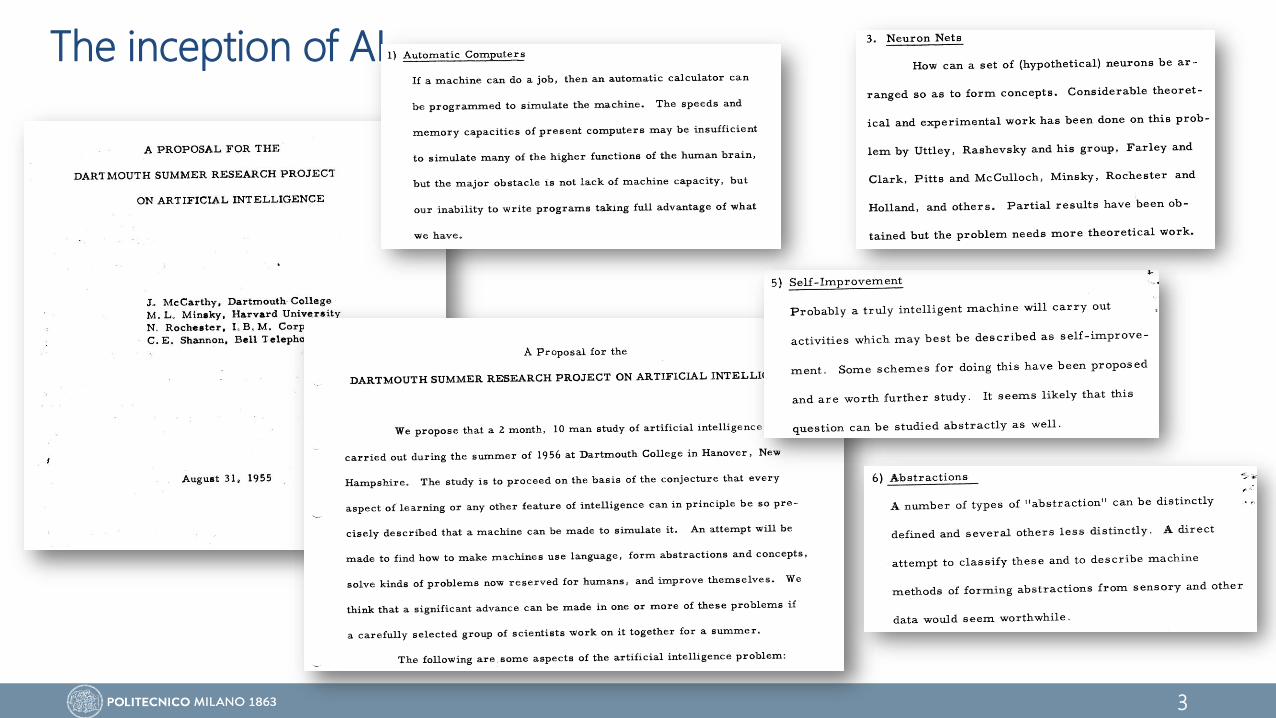
The inception of AI
4
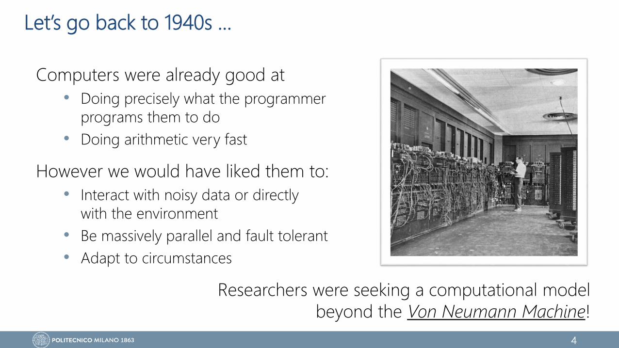
Let’s go back to 1940s ...
Computers were already good at
• Doing precisely what the programmer
programs them to do
• Doing arithmetic very fast
However we would have liked them to:
• Interact with noisy data or directly
with the environment
• Be massively parallel and fault tolerant
• Adapt to circumstances
Researchers were seeking a computational model
beyond the Von Neumann Machine!
5
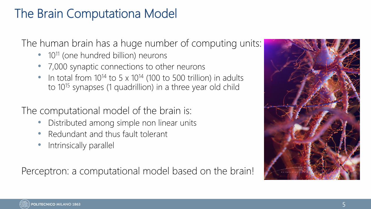
The Brain Computationa Model
The human brain has a huge number of computing units: • 1011 (one hundred billion) neurons
• 7,000 synaptic connections to other neurons
• In total from 1014 to 5 x 10¹⁴ (100 to 500 trillion) in adultsto 1015 synapses (1 quadrillion) in a three year old child
The computational model of the brain is:• Distributed among simple non linear units
• Redundant and thus fault tolerant
• Intrinsically parallel
Perceptron: a computational model based on the brain!

6
Computation in Biological Neurons
7
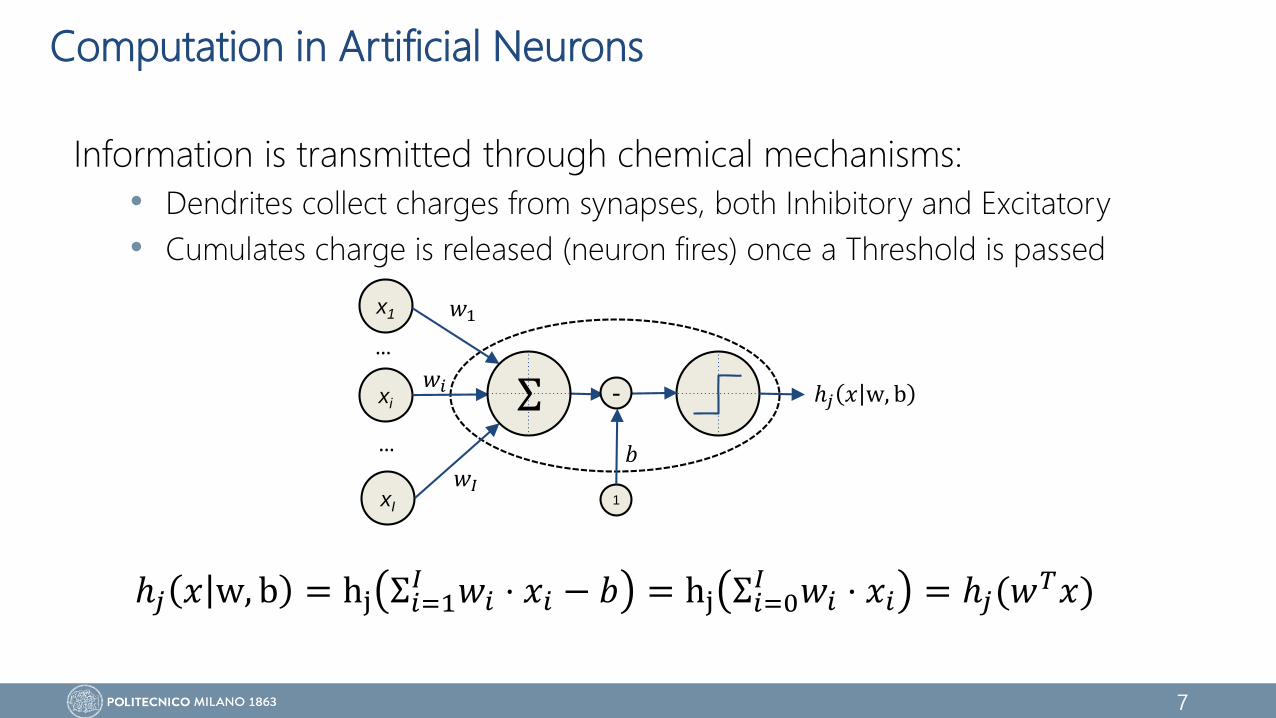
Computation in Artificial Neurons
Information is transmitted through chemical mechanisms:
• Dendrites collect charges from synapses, both Inhibitory and Excitatory
• Cumulates charge is released (neuron fires) once a Threshold is passed
x1
xI
xi
…
…
1
ℎ𝑗 𝑥 w, b𝑤𝑖
𝑤1
𝑤𝐼
𝑏
Σ -
ℎ𝑗 𝑥 w, b = hj Σ𝑖=1𝐼 𝑤𝑖 ⋅ 𝑥𝑖 − 𝑏 = hj Σ𝑖=0
𝐼 𝑤𝑖 ⋅ 𝑥𝑖 = ℎ𝑗(𝑤𝑇𝑥)
8
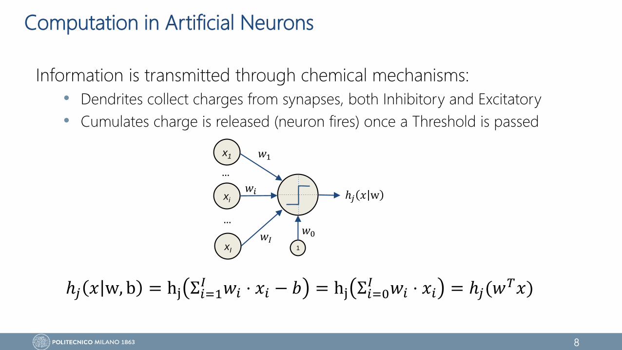
Computation in Artificial Neurons
Information is transmitted through chemical mechanisms:
• Dendrites collect charges from synapses, both Inhibitory and Excitatory
• Cumulates charge is released (neuron fires) once a Threshold is passed
ℎ𝑗 𝑥 w, b = hj Σ𝑖=1𝐼 𝑤𝑖 ⋅ 𝑥𝑖 − 𝑏 = hj Σ𝑖=0
𝐼 𝑤𝑖 ⋅ 𝑥𝑖 = ℎ𝑗(𝑤𝑇𝑥)
x1
xI
xi
…
…
1
ℎ𝑗 𝑥 w𝑤𝑖
𝑤1
𝑤𝐼𝑤0
9
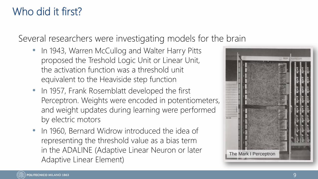
Who did it first?
Several researchers were investigating models for the brain
• In 1943, Warren McCullog and Walter Harry Pitts
proposed the Treshold Logic Unit or Linear Unit,
the activation function was a threshold unit
equivalent to the Heaviside step function
• In 1957, Frank Rosemblatt developed the first
Perceptron. Weights were encoded in potentiometers,
and weight updates during learning were performed
by electric motors
• In 1960, Bernard Widrow introduced the idea of
representing the threshold value as a bias term
in the ADALINE (Adaptive Linear Neuron or later
Adaptive Linear Element)The Mark I Perceptron
10
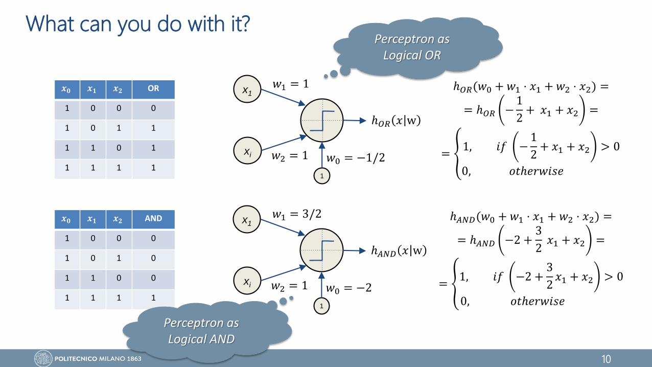
What can you do with it?
𝒙𝟎 𝒙𝟏 𝒙𝟐 OR
1 0 0 0
1 0 1 1
1 1 0 1
1 1 1 1
𝒙𝟎 𝒙𝟏 𝒙𝟐 AND
1 0 0 0
1 0 1 0
1 1 0 0
1 1 1 1
x1
xi
1
ℎ𝐴𝑁𝐷 𝑥 w
𝑤2 = 1
𝑤1 = 3/2
𝑤0 = −2
x1
xi
1
ℎ𝑂𝑅 𝑥 w
𝑤2 = 1
𝑤1 = 1
𝑤0 = −1/2
ℎ𝑂𝑅(𝑤0 + 𝑤1 ⋅ 𝑥1 + 𝑤2 ⋅ 𝑥2) =
= ℎ𝑂𝑅 −1
2+ 𝑥1 + 𝑥2 =
= 1, 𝑖𝑓 −
1
2+ 𝑥1 + 𝑥2 > 0
0, 𝑜𝑡ℎ𝑒𝑟𝑤𝑖𝑠𝑒
ℎ𝐴𝑁𝐷(𝑤0 + 𝑤1 ⋅ 𝑥1 + 𝑤2 ⋅ 𝑥2) =
= ℎ𝐴𝑁𝐷 −2 +3
2𝑥1 + 𝑥2 =
= 1, 𝑖𝑓 −2 +
3
2𝑥1 + 𝑥2 > 0
0, 𝑜𝑡ℎ𝑒𝑟𝑤𝑖𝑠𝑒
Perceptron as Logical OR
Perceptron as Logical AND
11
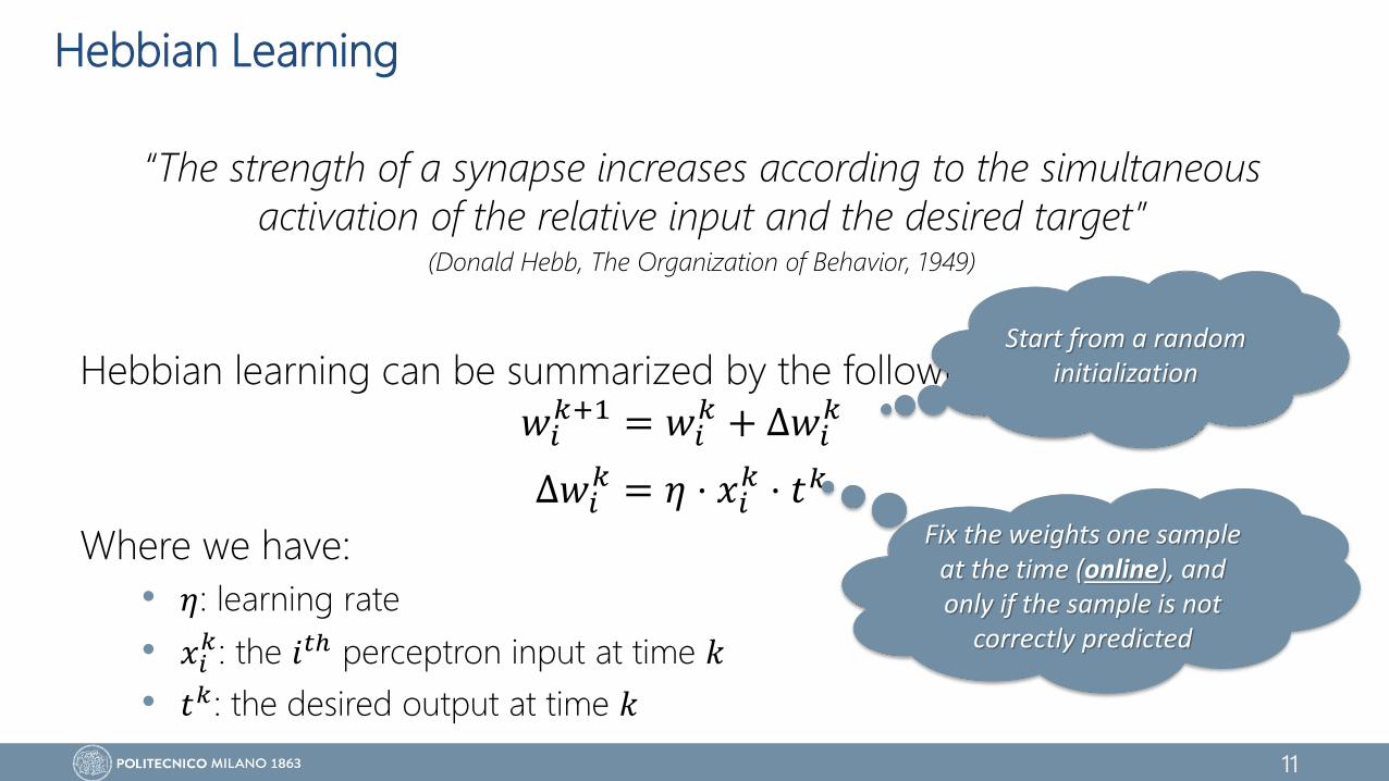
Hebbian Learning
“The strength of a synapse increases according to the simultaneous
activation of the relative input and the desired target” (Donald Hebb, The Organization of Behavior, 1949)
Hebbian learning can be summarized by the following rule:
Where we have:
• 𝜂: learning rate
• 𝑥𝑖𝑘: the 𝑖𝑡ℎ perceptron input at time 𝑘
• 𝑡𝑘 : the desired output at time 𝑘
𝑤𝑖𝑘+1 = 𝑤𝑖
𝑘 + Δ𝑤𝑖𝑘
Δ𝑤𝑖𝑘 = 𝜂 ⋅ 𝑥𝑖
𝑘 ⋅ 𝑡𝑘
Fix the weights one sample at the time (online), and only if the sample is not
correctly predicted
Start from a random initialization
12
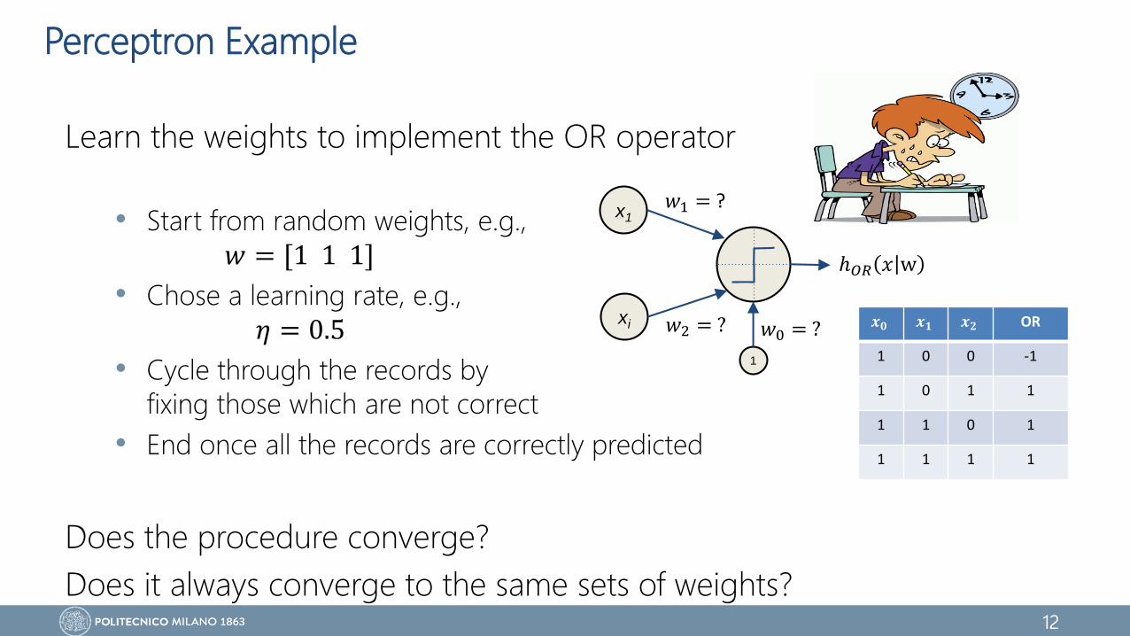
Perceptron Example
Learn the weights to implement the OR operator
• Start from random weights, e.g.,
𝑤 = [1 1 1]
• Chose a learning rate, e.g.,
𝜂 = 0.5
• Cycle through the records by
fixing those which are not correct
• End once all the records are correctly predicted
Does the procedure converge?
Does it always converge to the same sets of weights?
𝒙𝟎 𝒙𝟏 𝒙𝟐 OR
1 0 0 -1
1 0 1 1
1 1 0 1
1 1 1 1
x1
xi
1
ℎ𝑂𝑅 𝑥 w
𝑤2 = ?
𝑤1 = ?
𝑤0 = ?
13
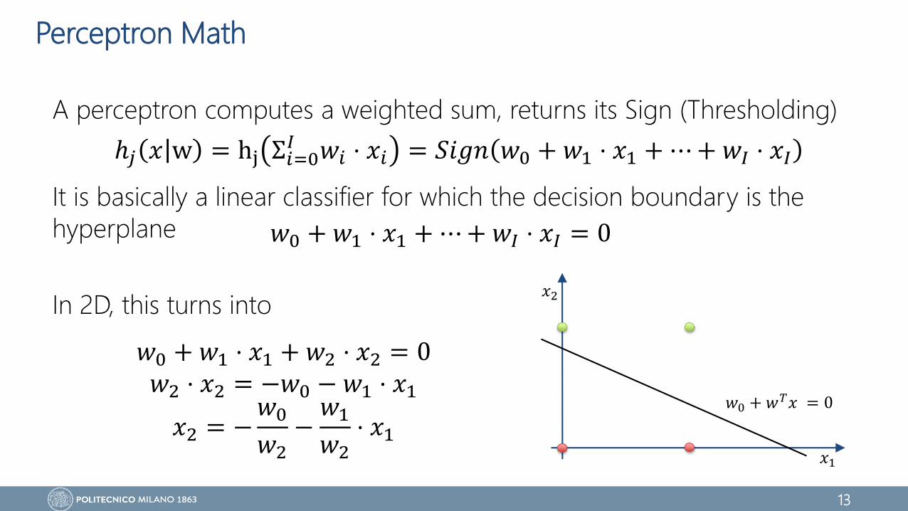
Perceptron Math
A perceptron computes a weighted sum, returns its Sign (Thresholding)
It is basically a linear classifier for which the decision boundary is the
hyperplane
In 2D, this turns into
ℎ𝑗 𝑥 w = hj Σ𝑖=0𝐼 𝑤𝑖 ⋅ 𝑥𝑖 = 𝑆𝑖𝑔𝑛 𝑤0 + 𝑤1 ⋅ 𝑥1 + ⋯ + 𝑤𝐼 ⋅ 𝑥𝐼
𝑤0 + 𝑤1 ⋅ 𝑥1 + ⋯ + 𝑤𝐼 ⋅ 𝑥𝐼 = 0
𝑤0 + 𝑤1 ⋅ 𝑥1 + 𝑤2 ⋅ 𝑥2 = 0𝑤2 ⋅ 𝑥2 = −𝑤0 − 𝑤1 ⋅ 𝑥1
𝑥2 = −𝑤0
𝑤2−
𝑤1
𝑤2⋅ 𝑥1
𝑥1
𝑤0 + 𝑤𝑇𝑥 = 0
𝑥2
14
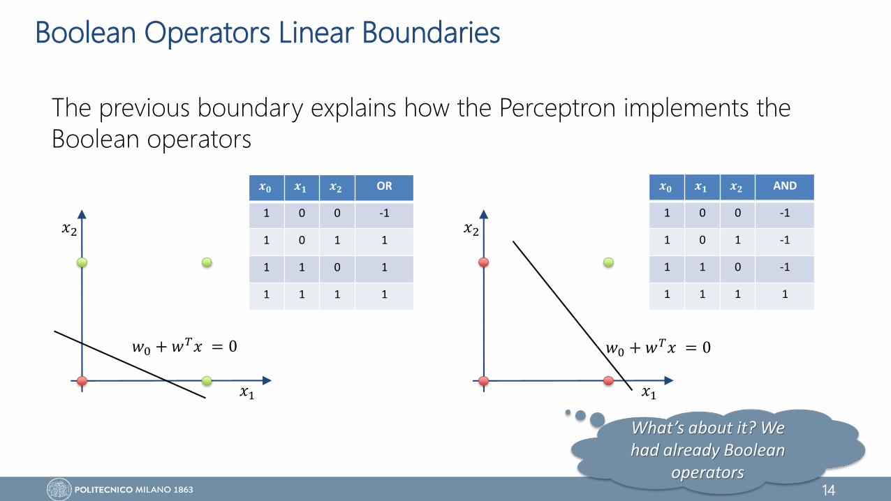
Boolean Operators Linear Boundaries
The previous boundary explains how the Perceptron implements the
Boolean operators
𝑥1
𝑤0 + 𝑤𝑇𝑥 = 0
𝑥2
𝑥1
𝑤0 + 𝑤𝑇𝑥 = 0
𝑥2
𝒙𝟎 𝒙𝟏 𝒙𝟐 OR
1 0 0 -1
1 0 1 1
1 1 0 1
1 1 1 1
𝒙𝟎 𝒙𝟏 𝒙𝟐 AND
1 0 0 -1
1 0 1 -1
1 1 0 -1
1 1 1 1
What’s about it? We had already Boolean
operators
15
What can’t you do with it?
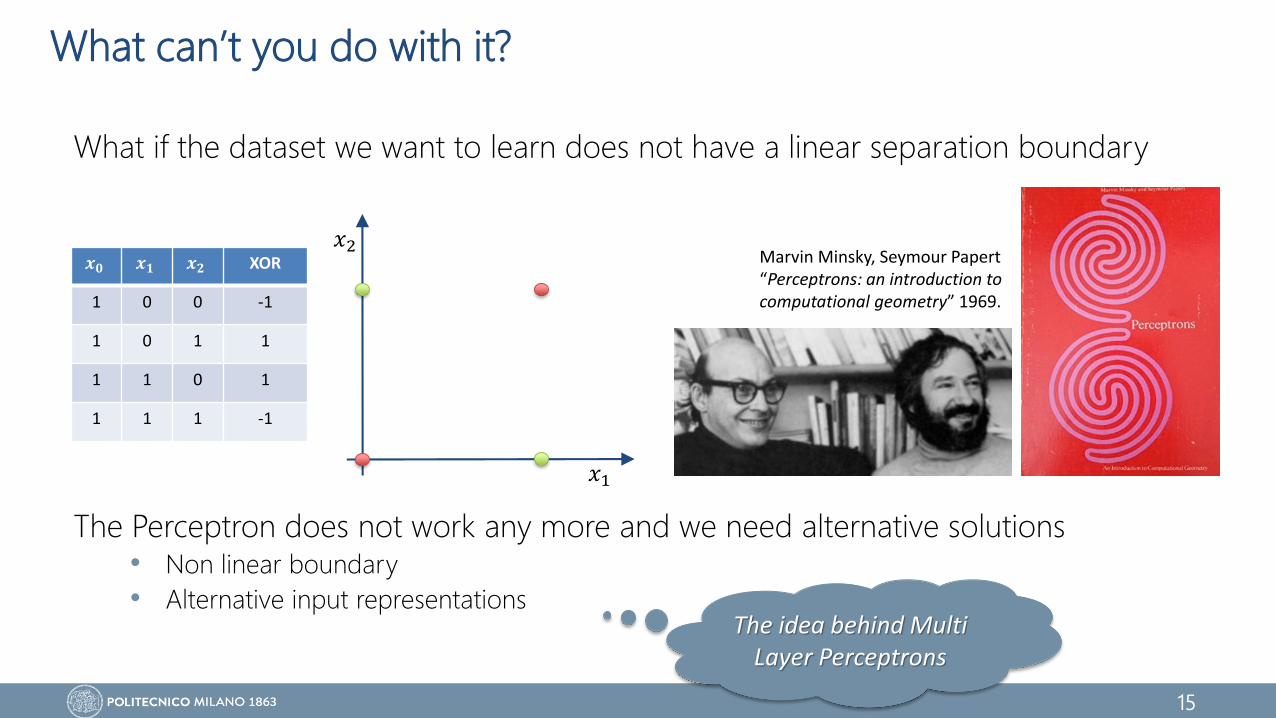
What if the dataset we want to learn does not have a linear separation boundary
The Perceptron does not work any more and we need alternative solutions• Non linear boundary
• Alternative input representations
𝑥1
𝑥2𝒙𝟎 𝒙𝟏 𝒙𝟐 XOR
1 0 0 -1
1 0 1 1
1 1 0 1
1 1 1 -1
Marvin Minsky, Seymour Papert“Perceptrons: an introduction to computational geometry” 1969.
The idea behind Multi Layer Perceptrons
16
What can’t you do with it?
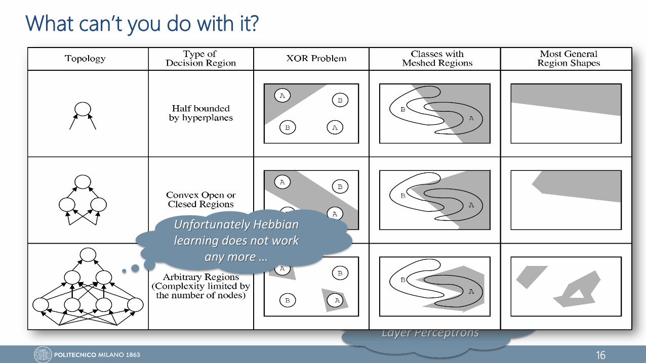
What if the dataset we want to learn does not have a linear separation boundary
The Perceptron does not work any more and we need alternative solutions• Non linear boundary
• Alternative input representations
𝑥1
𝑥2𝒙𝟎 𝒙𝟏 𝒙𝟐 XOR
1 0 0 0
1 0 1 1
1 1 0 1
1 1 1 0
Marvin Minsky, Seymour Papert“Perceptrons: an introduction to computational geometry” 1969.
The idea behind Multi Layer Perceptrons
Unfortunately Hebbianlearning does not work
any more …
17
Feed Forward Neural Networks
x1
xI
xi
…
…
1
𝑔1 𝑥 w𝑤𝑗𝑖
𝑤11
𝑤𝐽𝐼
𝑤10
… … …
…
1 1
𝑔𝐾 𝑥 w
1
Input Layer(I neurons)
Output Layer(K neurons)
Hidden Layer 1(J1 neurons)
Hidden Layer 2(J2 neurons)
Hidden Layer 3(J3 neurons)
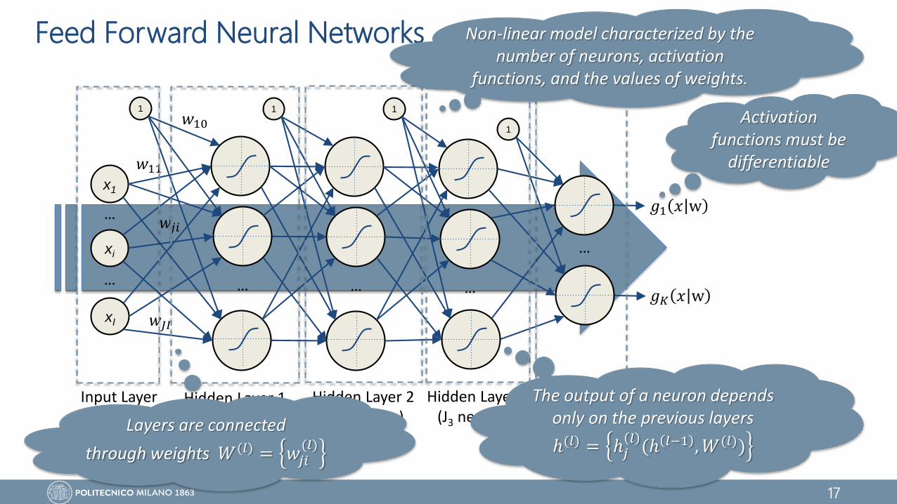
Non-linear model characterized by the number of neurons, activation
functions, and the values of weights.
Layers are connected
through weights 𝑊(𝑙) = 𝑤𝑗𝑖(𝑙)
The output of a neuron depends only on the previous layers
ℎ(𝑙) = ℎ𝑗𝑙(ℎ 𝑙−1 , 𝑊(𝑙))
Activation functions must be
differentiable
18
Which Activation Function?
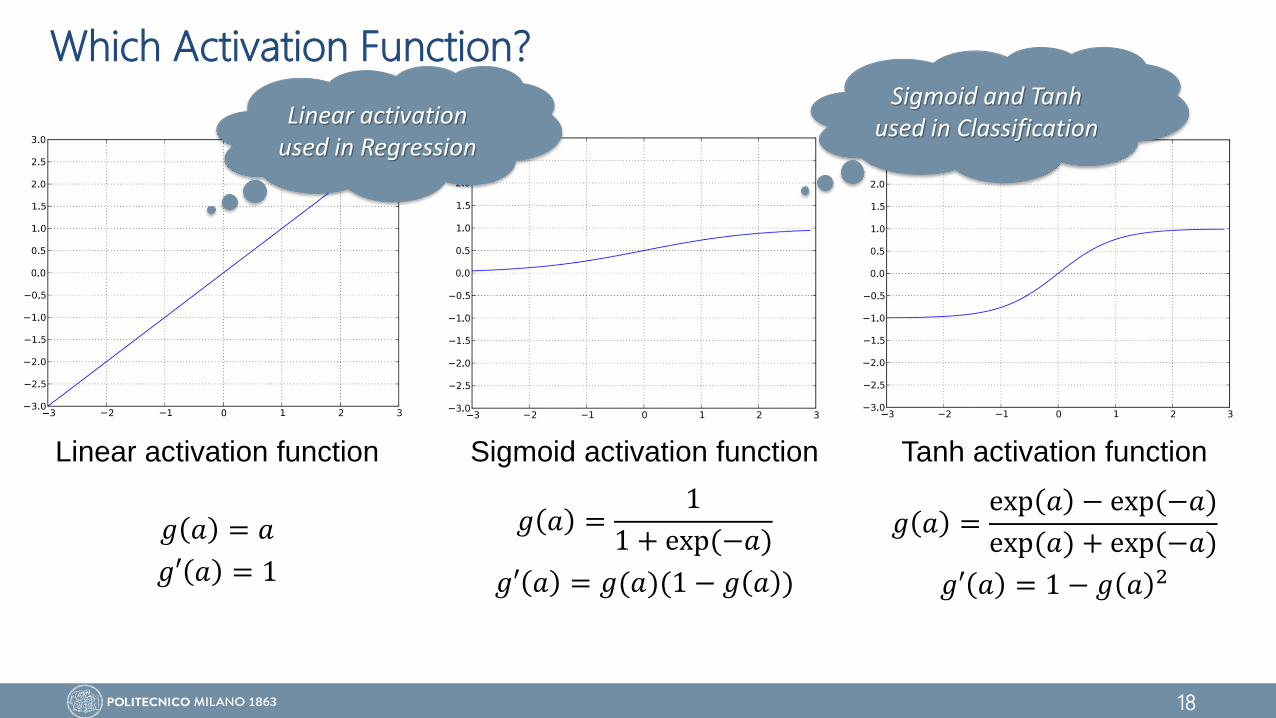
Linear activation function
𝑔 𝑎 = 𝑎
𝑔′ 𝑎 = 1
Sigmoid activation function
𝑔 𝑎 =1
1 + exp(−𝑎)
𝑔′ 𝑎 = 𝑔(𝑎)(1 − 𝑔 𝑎 )
Tanh activation function
𝑔 𝑎 =exp 𝑎 − exp(−𝑎)
exp(𝑎) + exp(−𝑎)
𝑔′ 𝑎 = 1 − 𝑔 𝑎 2
Linear activation used in Regression
Sigmoid and Tanh used in Classification
19
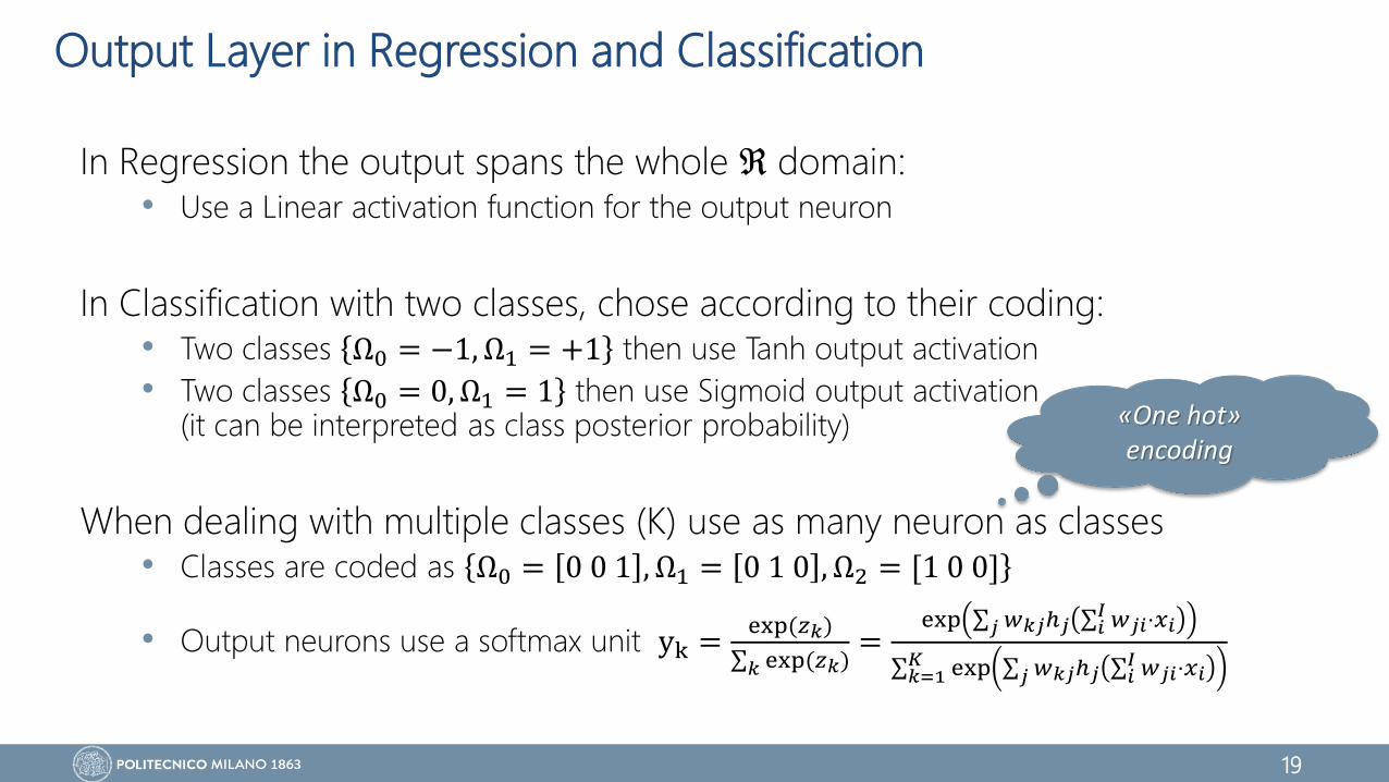
Output Layer in Regression and Classification
In Regression the output spans the whole ℜ domain:• Use a Linear activation function for the output neuron
In Classification with two classes, chose according to their coding:• Two classes Ω0 = −1, Ω1 = +1 then use Tanh output activation
• Two classes Ω0 = 0, Ω1 = 1 then use Sigmoid output activation (it can be interpreted as class posterior probability)
When dealing with multiple classes (K) use as many neuron as classes• Classes are coded as Ω0 = 0 0 1 , Ω1 = 0 1 0 , Ω2 = [1 0 0]
• Output neurons use a softmax unit yk =exp(𝑧𝑘)
𝑘 exp(𝑧𝑘)=
exp 𝑗 𝑤𝑘𝑗ℎ𝑗 𝑖𝐼 𝑤𝑗𝑖⋅𝑥𝑖
𝑘=1𝐾 exp 𝑗 𝑤𝑘𝑗ℎ𝑗 𝑖
𝐼 𝑤𝑗𝑖⋅𝑥𝑖
«One hot» encoding
20
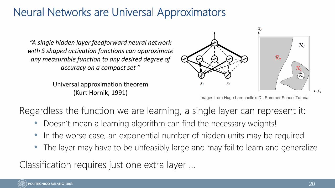
Regardless the function we are learning, a single layer can represent it:
• Doesn’t mean a learning algorithm can find the necessary weights!
• In the worse case, an exponential number of hidden units may be required
• The layer may have to be unfeasibly large and may fail to learn and generalize
Classification requires just one extra layer …
Images from Hugo Larochelle’s DL Summer School Tutorial
Neural Networks are Universal Approximators
“A single hidden layer feedforward neural network with S shaped activation functions can approximate any measurable function to any desired degree of
accuracy on a compact set ”
Universal approximation theorem(Kurt Hornik, 1991)
21
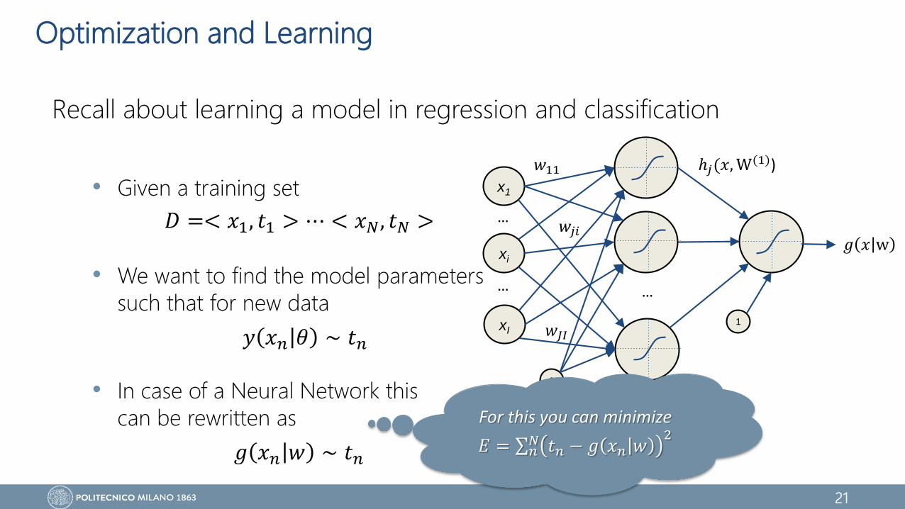
Optimization and Learning
Recall about learning a model in regression and classification
• Given a training set
• We want to find the model parameters
such that for new data
• In case of a Neural Network this
can be rewritten as
x1
xI
xi
…
…
𝑔 𝑥 w𝑤𝑗𝑖
𝑤11
𝑤𝐽𝐼
…
ℎ𝑗(𝑥, W(1))
1
1
𝐷 =< 𝑥1, 𝑡1 > ⋯ < 𝑥𝑁, 𝑡𝑁 >
𝑦 𝑥𝑛 𝜃 ∼ 𝑡𝑛
𝑔 𝑥𝑛 𝑤 ∼ 𝑡𝑛
For this you can minimize
𝐸 = 𝑛𝑁 𝑡𝑛 − 𝑔 𝑥𝑛 𝑤
2
22
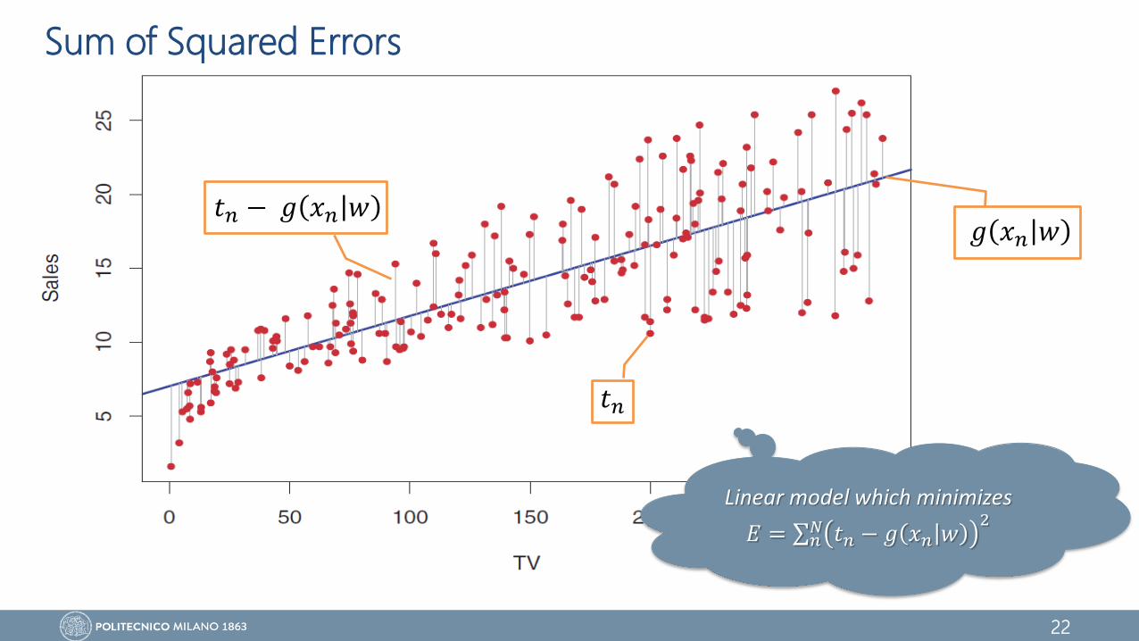
Sum of Squared Errors
𝑔 𝑥𝑛 𝑤
𝑡𝑛
Linear model which minimizes
𝐸 = 𝑛𝑁 𝑡𝑛 − 𝑔 𝑥𝑛 𝑤
2
𝑡𝑛 − 𝑔 𝑥𝑛 𝑤
23
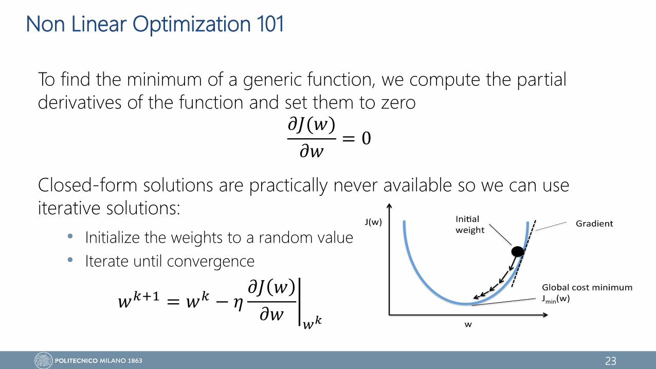
Non Linear Optimization 101
To find the minimum of a generic function, we compute the partial
derivatives of the function and set them to zero
Closed-form solutions are practically never available so we can use
iterative solutions:
• Initialize the weights to a random value
• Iterate until convergence
𝜕𝐽(𝑤)
𝜕𝑤= 0
𝑤𝑘+1 = 𝑤𝑘 − 𝜂 𝜕𝐽 𝑤
𝜕𝑤𝑤𝑘
24
𝑤
𝐸(𝑤)
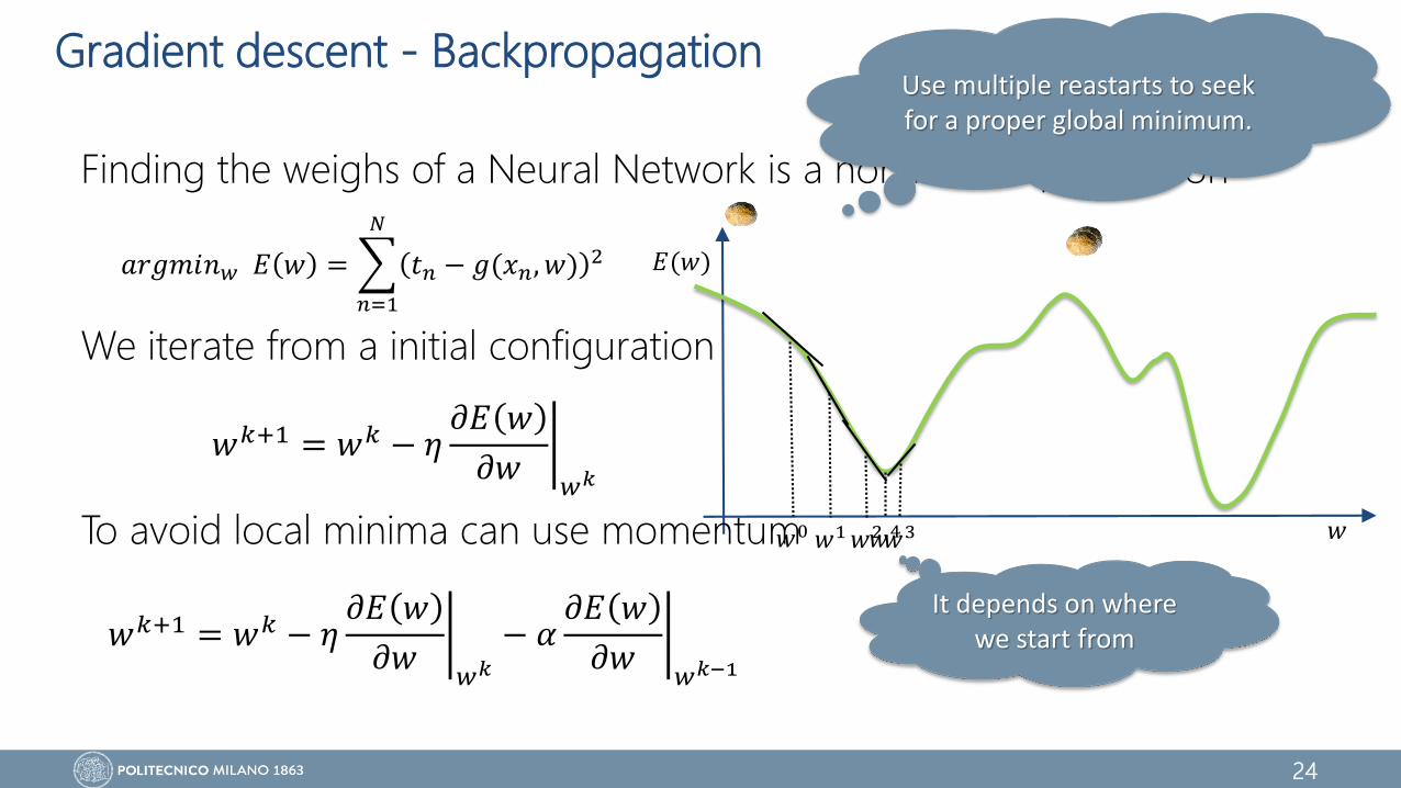
Gradient descent - Backpropagation
Finding the weighs of a Neural Network is a non linear optimization
We iterate from a initial configuration
To avoid local minima can use momentum
𝑎𝑟𝑔𝑚𝑖𝑛𝑤 𝐸 𝑤 =
𝑛=1
𝑁
𝑡𝑛 − 𝑔(𝑥𝑛, 𝑤) 2
𝑤0 𝑤1 𝑤2𝑤3𝑤4
𝑤𝑘+1 = 𝑤𝑘 − 𝜂 𝜕𝐸 𝑤
𝜕𝑤𝑤𝑘
𝑤𝑘+1 = 𝑤𝑘 − 𝜂 𝜕𝐸 𝑤
𝜕𝑤𝑤𝑘
− 𝛼 𝜕𝐸 𝑤
𝜕𝑤𝑤𝑘−1
It depends on where we start from
Use multiple reastarts to seek for a proper global minimum.
25
x1
xI
xi
…
…
𝑔 𝑥 w𝑤𝑗𝑖
(1)
𝑤11(1)
𝑤𝐽𝐼(1)
…
ℎ𝑗(𝑥, W(1))
1
1
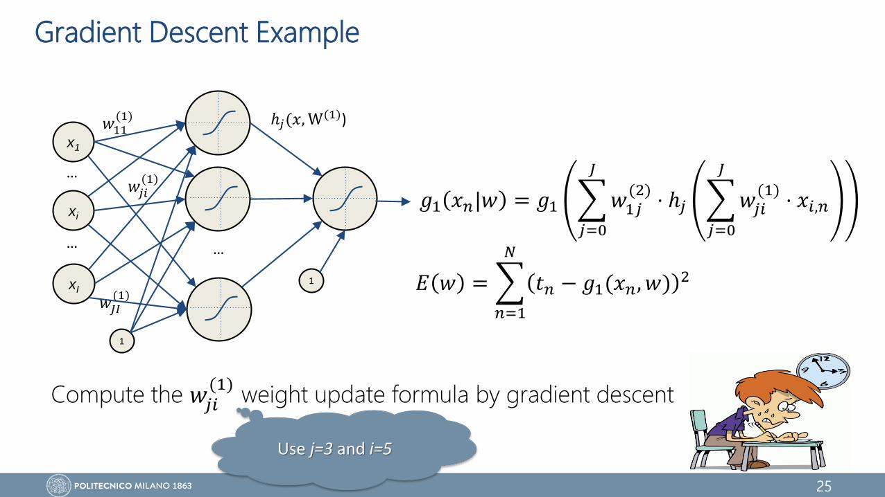
Gradient Descent Example
Compute the 𝑤𝑗𝑖(1)
weight update formula by gradient descent
𝐸 𝑤 =
𝑛=1
𝑁
𝑡𝑛 − 𝑔1(𝑥𝑛, 𝑤) 2
𝑔1 𝑥𝑛|𝑤 = 𝑔1
𝑗=0
𝐽
𝑤1𝑗(2)
⋅ ℎ𝑗
𝑗=0
𝐽
𝑤𝑗𝑖(1)
⋅ 𝑥𝑖,𝑛
Use j=3 and i=5
26
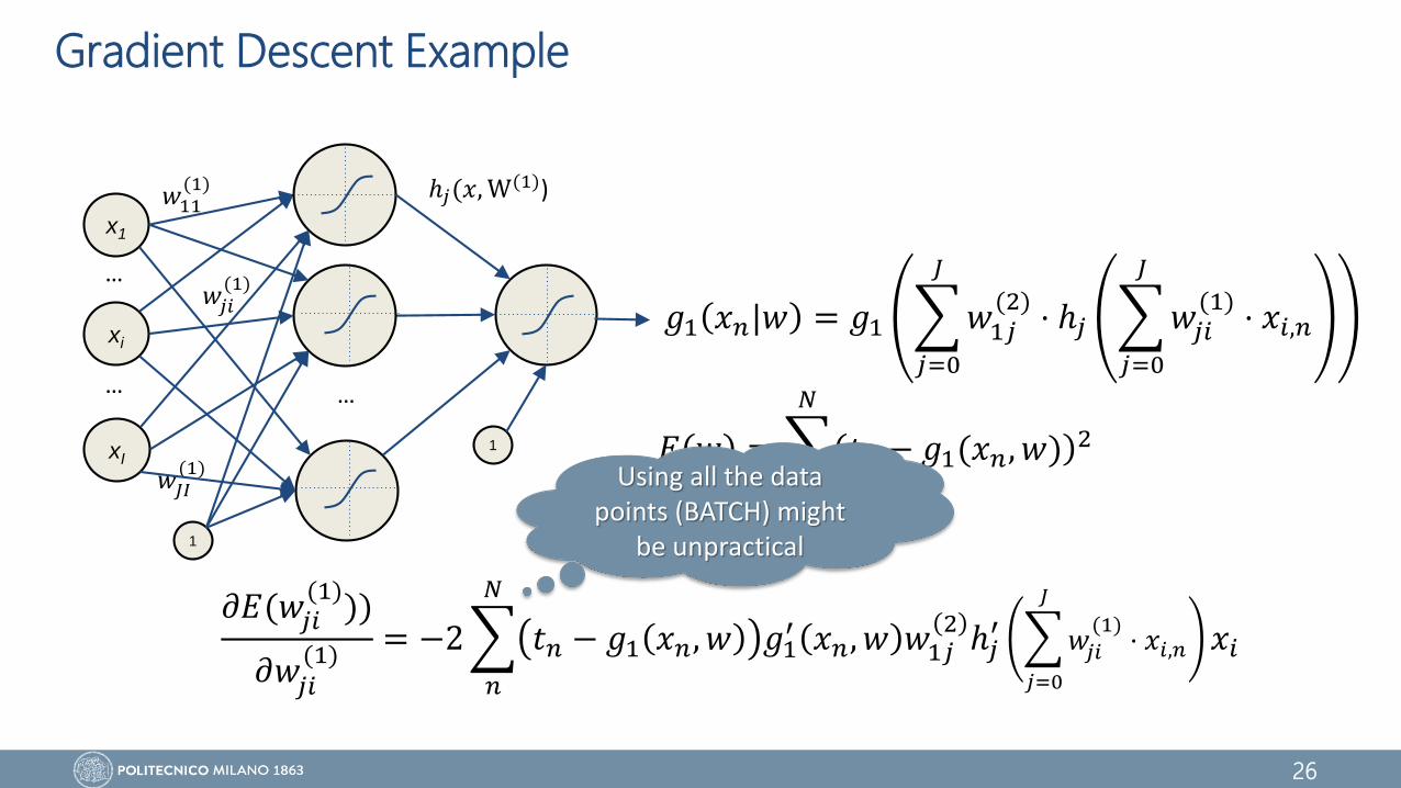
Gradient Descent Example
x1
xI
xi
…
…
𝑔 𝑥 w𝑤𝑗𝑖
(1)
𝑤11(1)
𝑤𝐽𝐼(1)
…
ℎ𝑗(𝑥, W(1))
1
1
𝐸 𝑤 =
𝑛=1
𝑁
𝑡𝑛 − 𝑔1(𝑥𝑛, 𝑤) 2
𝑔1 𝑥𝑛|𝑤 = 𝑔1
𝑗=0
𝐽
𝑤1𝑗(2)
⋅ ℎ𝑗
𝑗=0
𝐽
𝑤𝑗𝑖(1)
⋅ 𝑥𝑖,𝑛
𝜕𝐸(𝑤𝑗𝑖(1)
))
𝜕𝑤𝑗𝑖(1)
= −2
𝑛
𝑁
𝑡𝑛 − 𝑔1 𝑥𝑛, 𝑤 𝑔1′ 𝑥𝑛, 𝑤 𝑤1𝑗
2ℎ𝑗
′
𝑗=0
𝐽
𝑤𝑗𝑖
(1)⋅ 𝑥𝑖,𝑛 𝑥𝑖
Using all the data points (BATCH) might
be unpractical
27
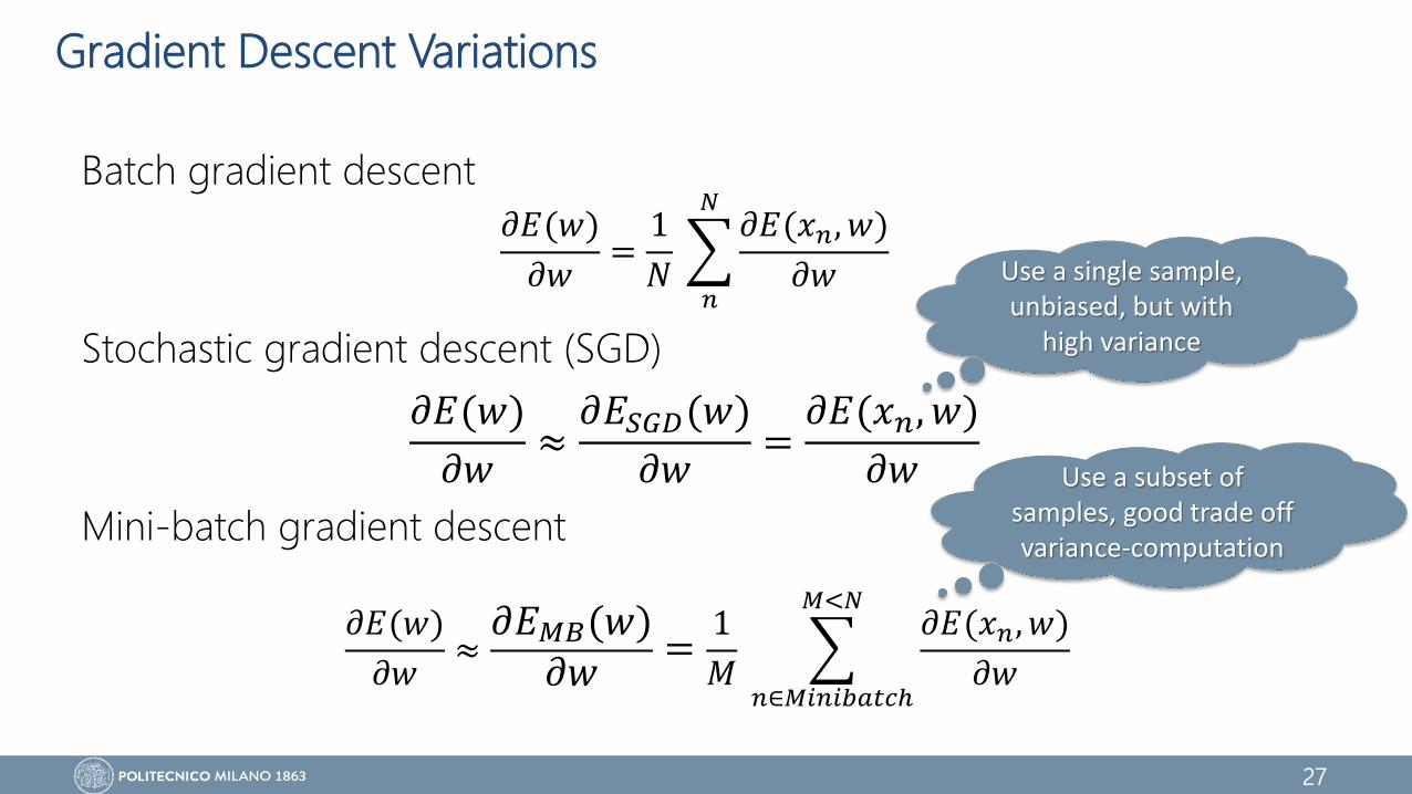
Gradient Descent Variations
Batch gradient descent
Stochastic gradient descent (SGD)
Mini-batch gradient descent
𝜕𝐸(𝑤)
𝜕𝑤=
1
𝑁
𝑛
𝑁𝜕𝐸(𝑥𝑛, 𝑤)
𝜕𝑤
𝜕𝐸(𝑤)
𝜕𝑤≈
𝜕𝐸𝑆𝐺𝐷(𝑤)
𝜕𝑤=
𝜕𝐸(𝑥𝑛, 𝑤)
𝜕𝑤
𝜕𝐸(𝑤)
𝜕𝑤≈
𝜕𝐸𝑀𝐵 𝑤𝜕𝑤
=1
𝑀
𝑛∈𝑀𝑖𝑛𝑖𝑏𝑎𝑡𝑐ℎ
𝑀<𝑁𝜕𝐸(𝑥𝑛, 𝑤)
𝜕𝑤
Use a single sample, unbiased, but with
high variance
Use a subset of samples, good trade off variance-computation
28
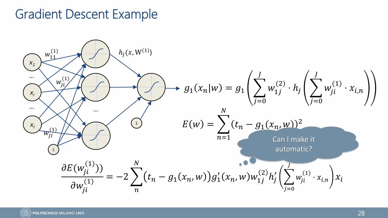
Gradient Descent Example
x1
xI
xi
…
…
𝑔 𝑥 w𝑤𝑗𝑖
(1)
𝑤11(1)
𝑤𝐽𝐼(1)
…
ℎ𝑗(𝑥, W(1))
1
1
𝐸 𝑤 =
𝑛=1
𝑁
𝑡𝑛 − 𝑔1(𝑥𝑛, 𝑤) 2
𝑔1 𝑥𝑛|𝑤 = 𝑔1
𝑗=0
𝐽
𝑤1𝑗(2)
⋅ ℎ𝑗
𝑗=0
𝐽
𝑤𝑗𝑖(1)
⋅ 𝑥𝑖,𝑛
𝜕𝐸(𝑤𝑗𝑖(1)
))
𝜕𝑤𝑗𝑖(1)
= −2
𝑛
𝑁
𝑡𝑛 − 𝑔1 𝑥𝑛, 𝑤 𝑔1′ 𝑥𝑛, 𝑤 𝑤1𝑗
2ℎ𝑗
′
𝑗=0
𝐽
𝑤𝑗𝑖
(1)⋅ 𝑥𝑖,𝑛 𝑥𝑖
Can I make it automatic?
29
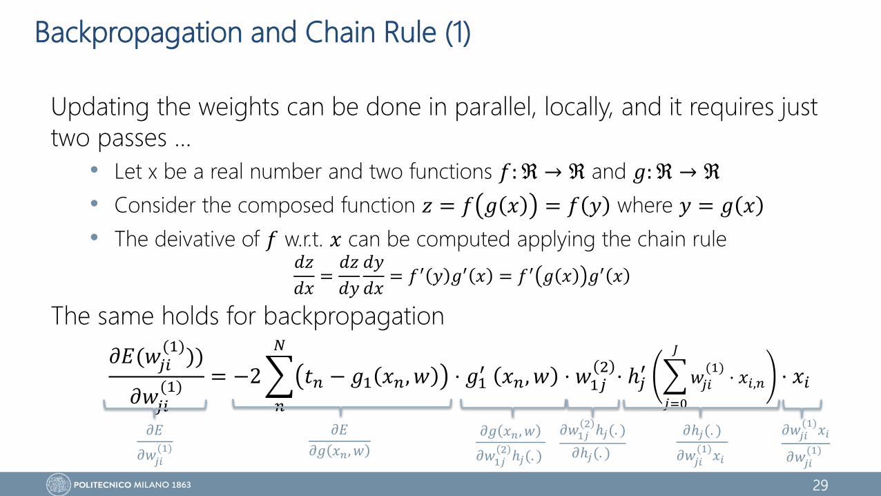
Backpropagation and Chain Rule (1)
Updating the weights can be done in parallel, locally, and it requires just
two passes ...
• Let x be a real number and two functions 𝑓: ℜ → ℜ and 𝑔: ℜ → ℜ
• Consider the composed function 𝑧 = 𝑓 𝑔 𝑥 = 𝑓 𝑦 where 𝑦 = 𝑔 𝑥
• The deivative of 𝑓 w.r.t. 𝑥 can be computed applying the chain rule
The same holds for backpropagation
𝑑𝑧
𝑑𝑥=
𝑑𝑧
𝑑𝑦
𝑑𝑦
𝑑𝑥= 𝑓′ 𝑦 𝑔′ 𝑥 = 𝑓′ 𝑔 𝑥 𝑔′ 𝑥
𝜕𝐸(𝑤𝑗𝑖(1)
))
𝜕𝑤𝑗𝑖(1)
= −2
𝑛
𝑁
𝑡𝑛 − 𝑔1 𝑥𝑛, 𝑤 ⋅ 𝑔1′ 𝑥𝑛, 𝑤 ⋅ 𝑤1𝑗
2⋅ ℎ𝑗
′
𝑗=0
𝐽
𝑤𝑗𝑖
(1)⋅ 𝑥𝑖,𝑛 ⋅ 𝑥𝑖
𝜕𝐸
𝜕𝑔 𝑥𝑛 , 𝑤
𝜕𝐸
𝜕𝑤𝑗𝑖(1)
𝜕𝑔 𝑥𝑛, 𝑤
𝜕𝑤1𝑗2
ℎ𝑗(. )
𝜕𝑤1𝑗2
ℎ𝑗(. )
𝜕ℎ𝑗(. )
𝜕ℎ𝑗(. )
𝜕𝑤𝑗𝑖(1)
𝑥𝑖
𝜕𝑤𝑗𝑖(1)
𝑥𝑖
𝜕𝑤𝑗𝑖(1)
30
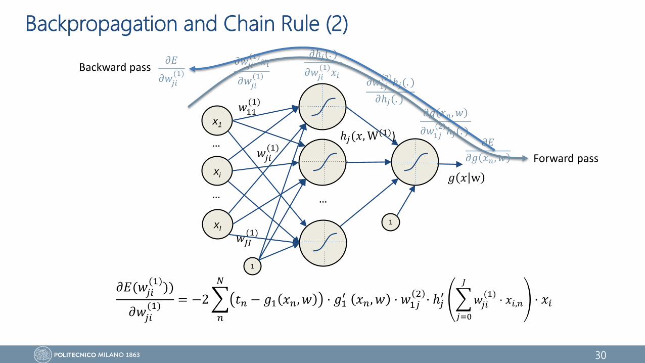
Backpropagation and Chain Rule (2)
𝜕𝐸(𝑤𝑗𝑖(1)
))
𝜕𝑤𝑗𝑖(1)
= −2
𝑛
𝑁
𝑡𝑛 − 𝑔1 𝑥𝑛, 𝑤 ⋅ 𝑔1′ 𝑥𝑛, 𝑤 ⋅ 𝑤1𝑗
2⋅ ℎ𝑗
′
𝑗=0
𝐽
𝑤𝑗𝑖(1)
⋅ 𝑥𝑖,𝑛 ⋅ 𝑥𝑖
x1
xI
xi
…
…
𝑔 𝑥 w
𝑤𝑗𝑖(1)
𝑤11(1)
𝑤𝐽𝐼(1)
…
ℎ𝑗(𝑥, W(1))
1
1
𝜕𝐸
𝜕𝑔 𝑥𝑛, 𝑤
𝜕𝑔 𝑥𝑛, 𝑤
𝜕𝑤1𝑗2
ℎ𝑗(. )
𝜕𝑤1𝑗2
ℎ𝑗(. )
𝜕ℎ𝑗(. )
𝜕ℎ𝑗(. )
𝜕𝑤𝑗𝑖(1)
𝑥𝑖
𝜕𝑤𝑗𝑖(1)
𝑥𝑖
𝜕𝑤𝑗𝑖(1)
Forward pass
𝜕𝐸
𝜕𝑤𝑗𝑖(1)
Backward pass
31
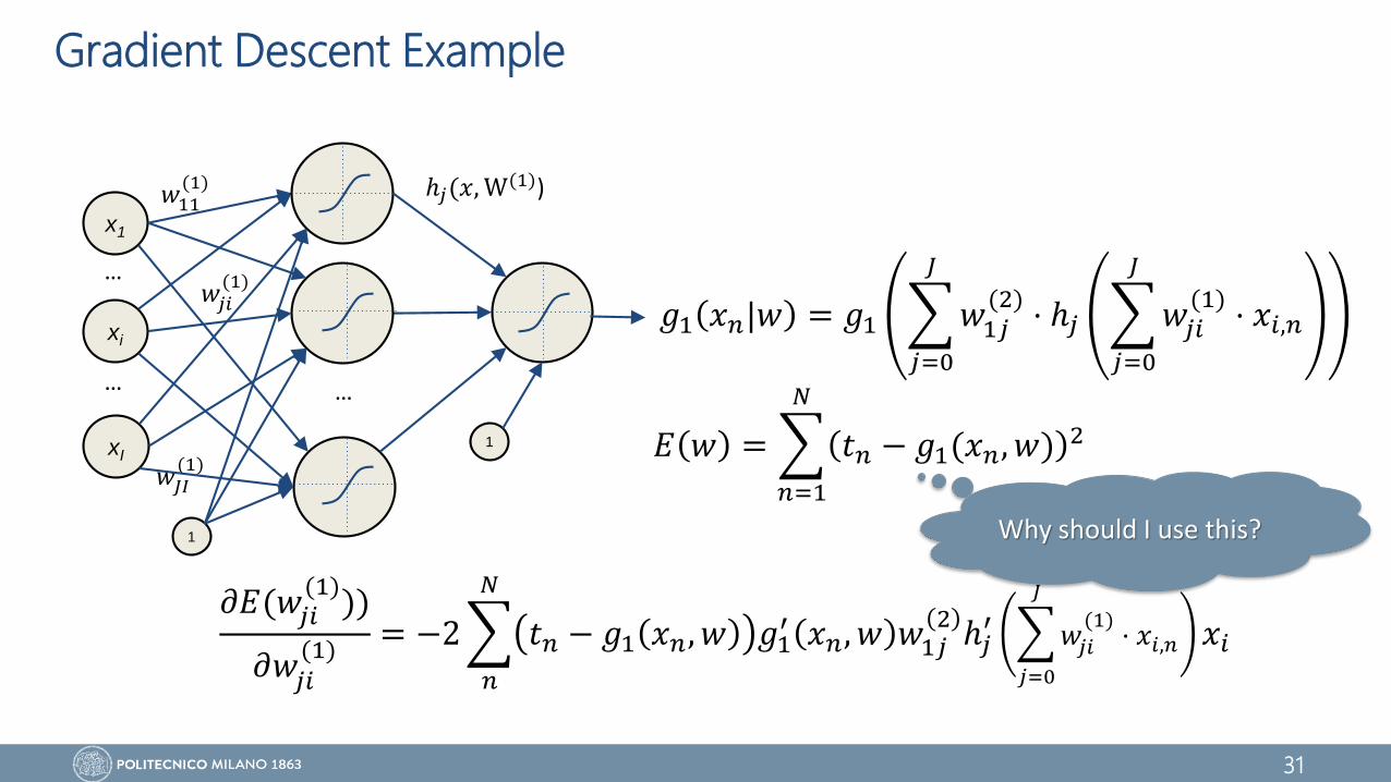
Gradient Descent Example
x1
xI
xi
…
…
𝑔 𝑥 w𝑤𝑗𝑖
(1)
𝑤11(1)
𝑤𝐽𝐼(1)
…
ℎ𝑗(𝑥, W(1))
1
1
𝐸 𝑤 =
𝑛=1
𝑁
𝑡𝑛 − 𝑔1(𝑥𝑛, 𝑤) 2
𝑔1 𝑥𝑛|𝑤 = 𝑔1
𝑗=0
𝐽
𝑤1𝑗(2)
⋅ ℎ𝑗
𝑗=0
𝐽
𝑤𝑗𝑖(1)
⋅ 𝑥𝑖,𝑛
𝜕𝐸(𝑤𝑗𝑖(1)
))
𝜕𝑤𝑗𝑖(1)
= −2
𝑛
𝑁
𝑡𝑛 − 𝑔1 𝑥𝑛, 𝑤 𝑔1′ 𝑥𝑛, 𝑤 𝑤1𝑗
2ℎ𝑗
′
𝑗=0
𝐽
𝑤𝑗𝑖
(1)⋅ 𝑥𝑖,𝑛 𝑥𝑖
Why should I use this?
32
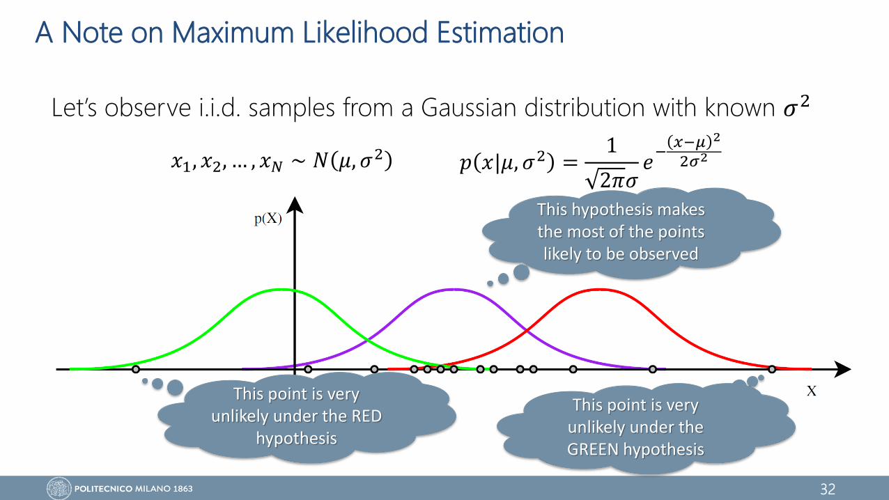
A Note on Maximum Likelihood Estimation
Let’s observe i.i.d. samples from a Gaussian distribution with known 𝜎2
𝑥1, 𝑥2, … , 𝑥𝑁 ∼ 𝑁 𝜇, 𝜎2 𝑝 𝑥|𝜇, 𝜎2 =1
2𝜋𝜎𝑒
−𝑥−𝜇 2
2𝜎2
This point is very unlikely under the RED
hypothesis
This point is very unlikely under the GREEN hypothesis
This hypothesis makes the most of the points likely to be observed
33
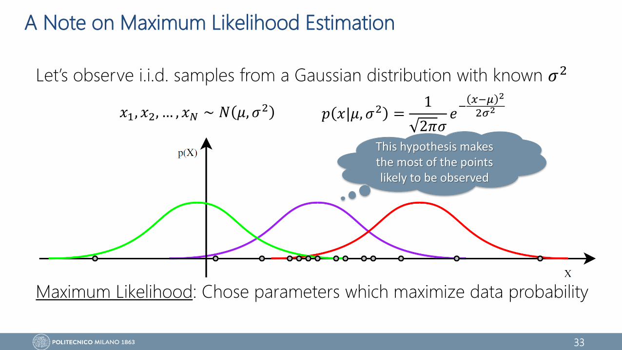
A Note on Maximum Likelihood Estimation
Let’s observe i.i.d. samples from a Gaussian distribution with known 𝜎2
Maximum Likelihood: Chose parameters which maximize data probability
𝑥1, 𝑥2, … , 𝑥𝑁 ∼ 𝑁 𝜇, 𝜎2 𝑝 𝑥|𝜇, 𝜎2 =1
2𝜋𝜎𝑒
−𝑥−𝜇 2
2𝜎2
This hypothesis makes the most of the points likely to be observed

34
Maximum Likelihood Estimation: The Recipe
Let 𝜃 = 𝜃1, 𝜃2, … , 𝜃𝑝𝑇
a vector of parameters, find the MLE for 𝜃:
• Write the likelihood 𝐿 = 𝑃 𝐷𝑎𝑡𝑎|𝜃 for the data
• [Take the logarithm of likelihood l = log 𝑃 𝐷𝑎𝑡𝑎|𝜃 ]
• Work out 𝜕𝐿
𝜕𝜃or
𝜕𝑙
𝜕𝜃using high-school calculus
• Solve the set of simultaneous equations 𝜕𝐿
𝜕𝜃𝑖= 0 or
𝜕𝑙
𝜕𝜃𝑖= 0
• Check that 𝜃𝑀𝐿𝐸 is a maximum
To maximize/minimize the (log)likelihood you can use:
• Analytical Techniques (i.e., solve the equations)
• Optimizaion Techniques (e.g., Lagrange mutipliers)
• Numerical Techniques (e.g., gradient descend)
We know already about gradient descent, let’s try
with some analitical stuff ...
Optional
35
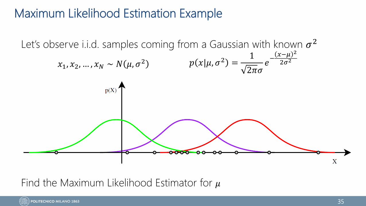
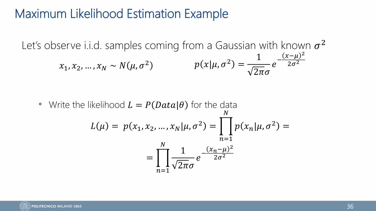
Maximum Likelihood Estimation Example
Let’s observe i.i.d. samples coming from a Gaussian with known 𝜎2
Find the Maximum Likelihood Estimator for 𝜇
𝑥1, 𝑥2, … , 𝑥𝑁 ∼ 𝑁 𝜇, 𝜎2 𝑝 𝑥|𝜇, 𝜎2 =1
2𝜋𝜎𝑒
−𝑥−𝜇 2
2𝜎2
36
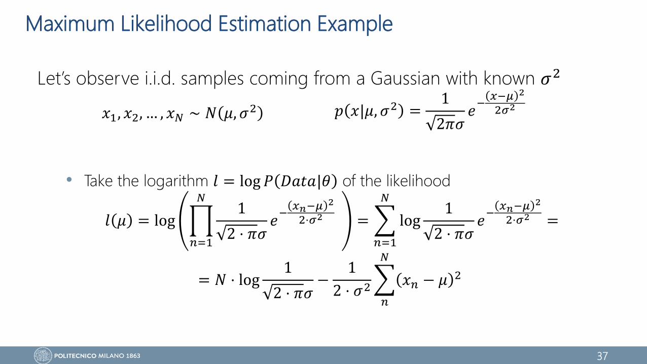
Maximum Likelihood Estimation Example
Let’s observe i.i.d. samples coming from a Gaussian with known 𝜎2
• Write the likelihood 𝐿 = 𝑃 𝐷𝑎𝑡𝑎|𝜃 for the data
𝑥1, 𝑥2, … , 𝑥𝑁 ∼ 𝑁 𝜇, 𝜎2 𝑝 𝑥|𝜇, 𝜎2 =1
2𝜋𝜎𝑒
−𝑥−𝜇 2
2𝜎2
𝐿 𝜇 = 𝑝 𝑥1, 𝑥2, … , 𝑥𝑁|𝜇, 𝜎2 =
𝑛=1
𝑁
𝑝 𝑥𝑛|𝜇, 𝜎2 =
=
𝑛=1
𝑁1
2𝜋𝜎𝑒
−𝑥𝑛−𝜇 2
2𝜎2
37
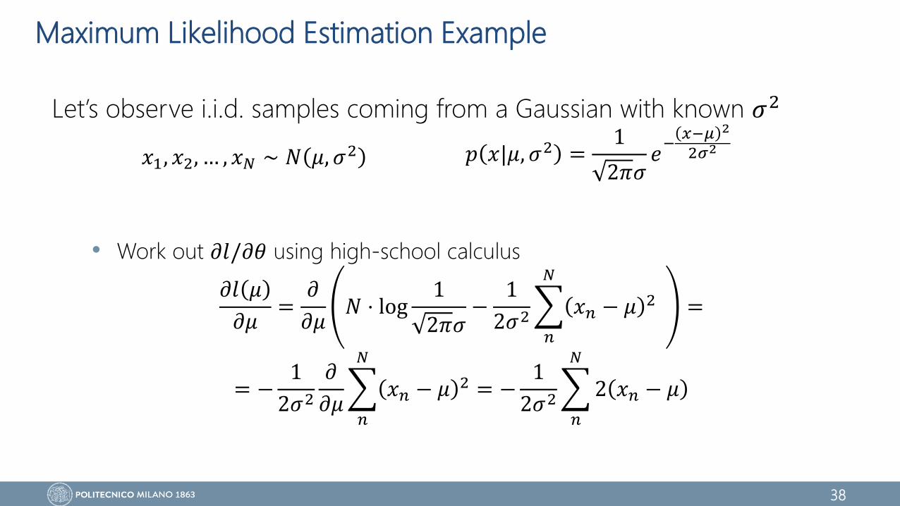
Maximum Likelihood Estimation Example
Let’s observe i.i.d. samples coming from a Gaussian with known 𝜎2
• Take the logarithm 𝑙 = log 𝑃 𝐷𝑎𝑡𝑎|𝜃 of the likelihood
𝑥1, 𝑥2, … , 𝑥𝑁 ∼ 𝑁 𝜇, 𝜎2 𝑝 𝑥|𝜇, 𝜎2 =1
2𝜋𝜎𝑒
−𝑥−𝜇 2
2𝜎2
𝑙 𝜇 = log
𝑛=1
𝑁1
2 ⋅ 𝜋𝜎𝑒
−𝑥𝑛−𝜇 2
2⋅𝜎2 =
𝑛=1
𝑁
log1
2 ⋅ 𝜋𝜎𝑒
−𝑥𝑛−𝜇 2
2⋅𝜎2 =
= 𝑁 ⋅ log1
2 ⋅ 𝜋𝜎−
1
2 ⋅ 𝜎2
𝑛
𝑁
𝑥𝑛 − 𝜇 2
38
Maximum Likelihood Estimation Example
Let’s observe i.i.d. samples coming from a Gaussian with known 𝜎2
• Work out 𝜕𝑙/𝜕𝜃 using high-school calculus
𝑥1, 𝑥2, … , 𝑥𝑁 ∼ 𝑁 𝜇, 𝜎2 𝑝 𝑥|𝜇, 𝜎2 =1
2𝜋𝜎𝑒
−𝑥−𝜇 2
2𝜎2
𝜕𝑙 𝜇
𝜕𝜇=
𝜕
𝜕𝜇𝑁 ⋅ log
1
2𝜋𝜎−
1
2𝜎2
𝑛
𝑁
𝑥𝑛 − 𝜇 2 =
= −1
2𝜎2
𝜕
𝜕𝜇
𝑛
𝑁
𝑥𝑛 − 𝜇 2 = −1
2𝜎2
𝑛
𝑁
2 𝑥𝑛 − 𝜇

39
Maximum Likelihood Estimation Example
Let’s observe i.i.d. samples coming from a Gaussian with known 𝜎2
• Solve the set of simultaneous equations 𝜕𝑙
𝜕𝜃𝑖= 0
𝑥1, 𝑥2, … , 𝑥𝑁 ∼ 𝑁 𝜇, 𝜎2 𝑝 𝑥|𝜇, 𝜎2 =1
2𝜋𝜎𝑒
−𝑥−𝜇 2
2𝜎2
−1
2𝜎2
𝑛
𝑁
2 𝑥𝑛 − 𝜇 = 0
𝑛
𝑁
𝑥𝑛 − 𝜇 = 0
𝑛
𝑁
𝑥𝑛 =
𝑛
𝑁
𝜇
Let’s apply this all toNeural Networks!
𝜇𝑀𝐿𝐸 =1
𝑁
𝑛
𝑁
𝑥𝑛
40
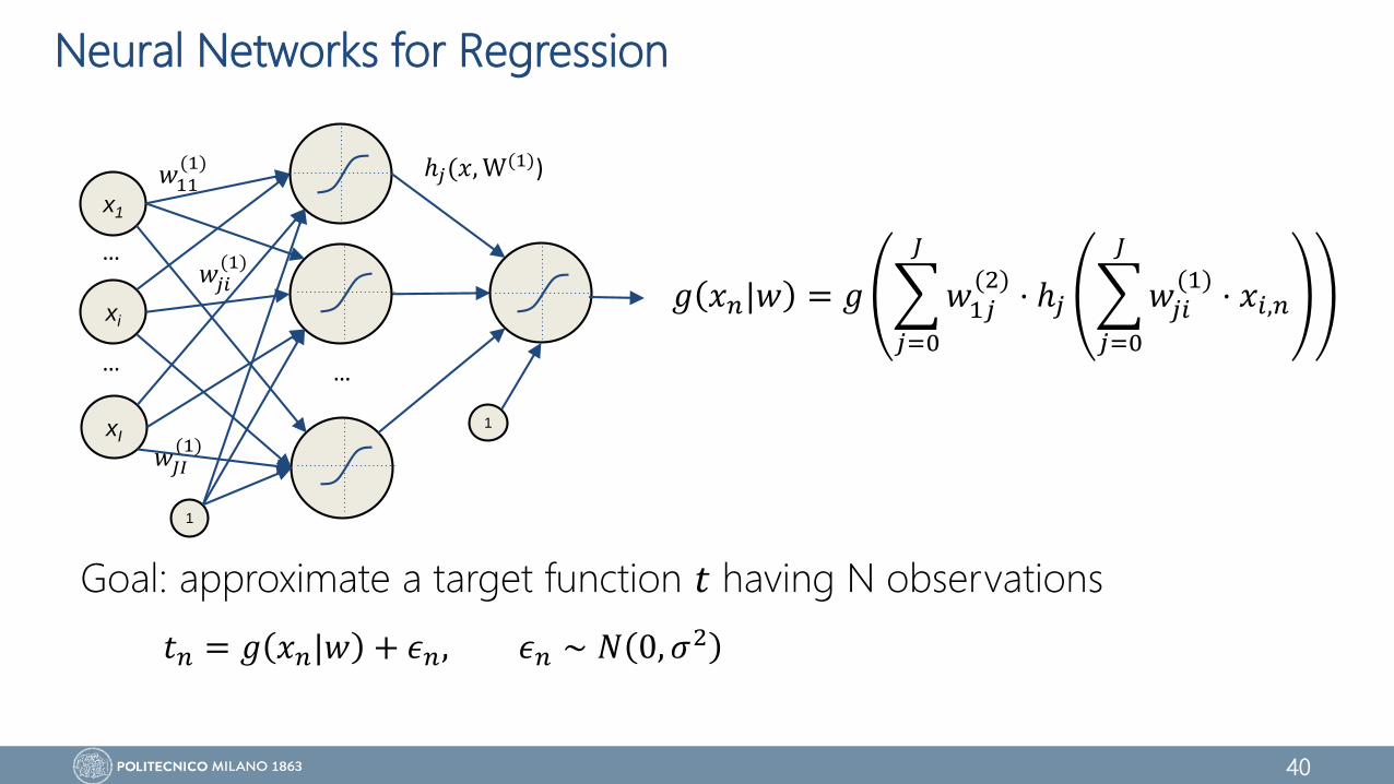
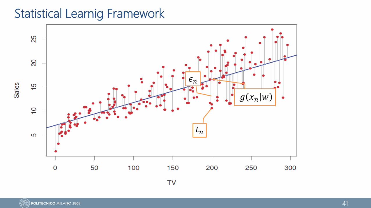
Neural Networks for Regression
Goal: approximate a target function 𝑡 having N observations
x1
xI
xi
…
…
𝑔 𝑥 w𝑤𝑗𝑖
(1)
𝑤11(1)
𝑤𝐽𝐼(1)
…
ℎ𝑗(𝑥, W(1))
1
1
𝑔 𝑥𝑛|𝑤 = 𝑔
𝑗=0
𝐽
𝑤1𝑗(2)
⋅ ℎ𝑗
𝑗=0
𝐽
𝑤𝑗𝑖(1)
⋅ 𝑥𝑖,𝑛
𝑡𝑛 = 𝑔 𝑥𝑛|𝑤 + 𝜖𝑛, 𝜖𝑛 ∼ 𝑁 0, 𝜎2
41
Statistical Learnig Framework
𝑔 𝑥𝑛 𝑤
𝑡𝑛
𝜖𝑛
42
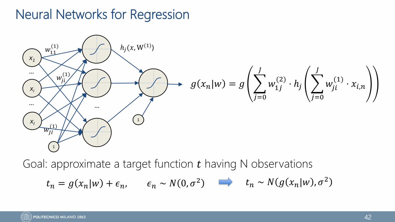
Neural Networks for Regression
Goal: approximate a target function 𝑡 having N observations
x1
xI
xi
…
…
𝑔 𝑥 w𝑤𝑗𝑖
(1)
𝑤11(1)
𝑤𝐽𝐼(1)
…
ℎ𝑗(𝑥, W(1))
1
1
𝑔 𝑥𝑛|𝑤 = 𝑔
𝑗=0
𝐽
𝑤1𝑗(2)
⋅ ℎ𝑗
𝑗=0
𝐽
𝑤𝑗𝑖(1)
⋅ 𝑥𝑖,𝑛
𝑡𝑛 = 𝑔 𝑥𝑛|𝑤 + 𝜖𝑛, 𝜖𝑛 ∼ 𝑁 0, 𝜎2 𝑡𝑛 ∼ 𝑁 𝑔 𝑥𝑛|𝑤 , 𝜎2

43
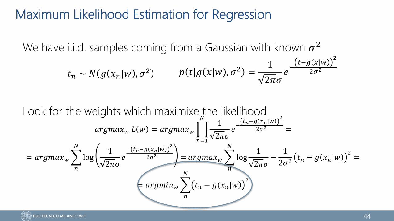
Maximum Likelihood Estimation for Regression
We have i.i.d. samples coming from a Gaussian with known 𝜎2
Write the likelihood 𝐿 = 𝑃 𝐷𝑎𝑡𝑎|𝜃 for the data
𝑝 𝑡|𝑔 𝑥|𝑤 , 𝜎2 =1
2𝜋𝜎𝑒
−𝑡−𝑔 𝑥|𝑤
2
2𝜎2
𝐿 𝑤 = 𝑝 𝑡1, 𝑡2, … , 𝑡𝑁|𝑔 𝑥|𝑤 , 𝜎2 =
𝑛=1
𝑁
𝑝 𝑡𝑛|𝑔 𝑥𝑛|𝑤 , 𝜎2 =
=
𝑛=1
𝑁1
2𝜋𝜎𝑒
−𝑡𝑛−𝑔 𝑥𝑛|𝑤
2
2𝜎2
𝑡𝑛 ∼ 𝑁 𝑔 𝑥𝑛|𝑤 , 𝜎2
44
Maximum Likelihood Estimation for Regression
We have i.i.d. samples coming from a Gaussian with known 𝜎2
Look for the weights which maximixe the likelihood
𝑝 𝑡|𝑔 𝑥|𝑤 , 𝜎2 =1
2𝜋𝜎𝑒
−𝑡−𝑔 𝑥|𝑤
2
2𝜎2
𝑎𝑟𝑔𝑚𝑎𝑥𝑤 𝐿 𝑤 = 𝑎𝑟𝑔𝑚𝑎𝑥𝑤
𝑛=1
𝑁1
2𝜋𝜎𝑒
−𝑡𝑛−𝑔 𝑥𝑛|𝑤
2
2𝜎2 =
= 𝑎𝑟𝑔𝑚𝑎𝑥𝑤
𝑛
𝑁
log1
2𝜋𝜎𝑒
−𝑡𝑛−𝑔 𝑥𝑛|𝑤
2
2𝜎2 = 𝑎𝑟𝑔𝑚𝑎𝑥𝑤
𝑛
𝑁
log1
2𝜋𝜎−
1
2𝜎2𝑡𝑛 − 𝑔 𝑥𝑛|𝑤
2=
= 𝑎𝑟𝑔𝑚𝑖𝑛𝑤
𝑛
𝑁
𝑡𝑛 − 𝑔 𝑥𝑛|𝑤2
𝑡𝑛 ∼ 𝑁 𝑔 𝑥𝑛|𝑤 , 𝜎2
45
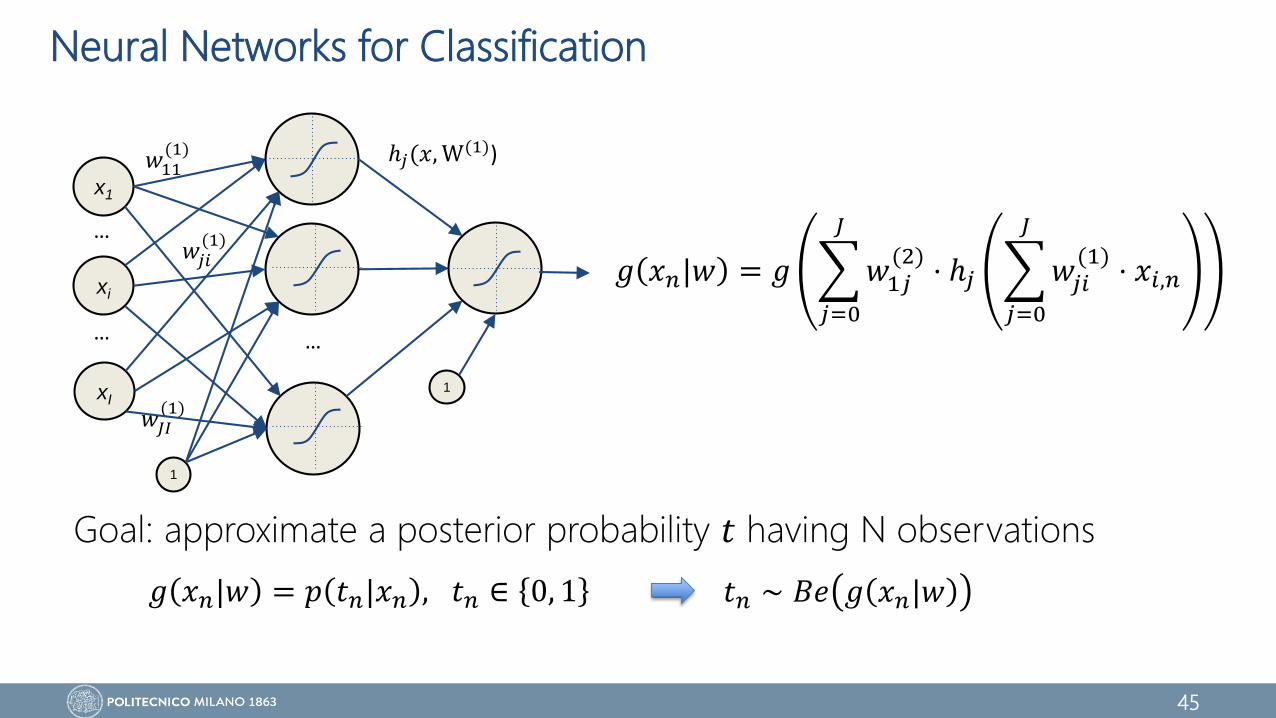
Neural Networks for Classification
Goal: approximate a posterior probability 𝑡 having N observations
x1
xI
xi
…
…
𝑔 𝑥 w𝑤𝑗𝑖
(1)
𝑤11(1)
𝑤𝐽𝐼(1)
…
ℎ𝑗(𝑥, W(1))
1
1
𝑔 𝑥𝑛|𝑤 = 𝑔
𝑗=0
𝐽
𝑤1𝑗(2)
⋅ ℎ𝑗
𝑗=0
𝐽
𝑤𝑗𝑖(1)
⋅ 𝑥𝑖,𝑛
𝑔 𝑥𝑛|𝑤 = 𝑝 𝑡𝑛|𝑥𝑛 , 𝑡𝑛 ∈ 0, 1 𝑡𝑛 ∼ 𝐵𝑒 𝑔 𝑥𝑛|𝑤
46
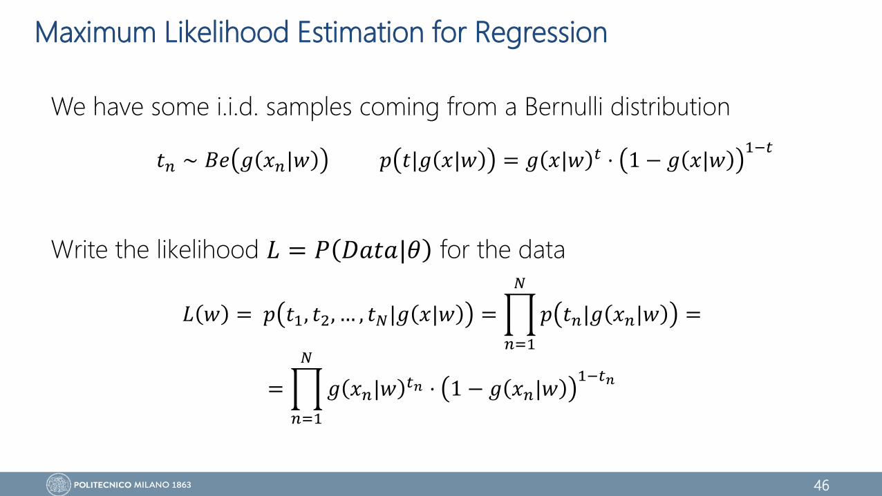
Maximum Likelihood Estimation for Regression
We have some i.i.d. samples coming from a Bernulli distribution
Write the likelihood 𝐿 = 𝑃 𝐷𝑎𝑡𝑎|𝜃 for the data
𝑝 𝑡|𝑔 𝑥|𝑤 = 𝑔 𝑥|𝑤 𝑡 ⋅ 1 − 𝑔 𝑥|𝑤1−𝑡
𝐿 𝑤 = 𝑝 𝑡1, 𝑡2, … , 𝑡𝑁|𝑔 𝑥|𝑤 =
𝑛=1
𝑁
𝑝 𝑡𝑛|𝑔 𝑥𝑛|𝑤 =
=
𝑛=1
𝑁
𝑔 𝑥𝑛|𝑤 𝑡𝑛 ⋅ 1 − 𝑔 𝑥𝑛|𝑤1−𝑡𝑛
𝑡𝑛 ∼ 𝐵𝑒 𝑔 𝑥𝑛|𝑤
47
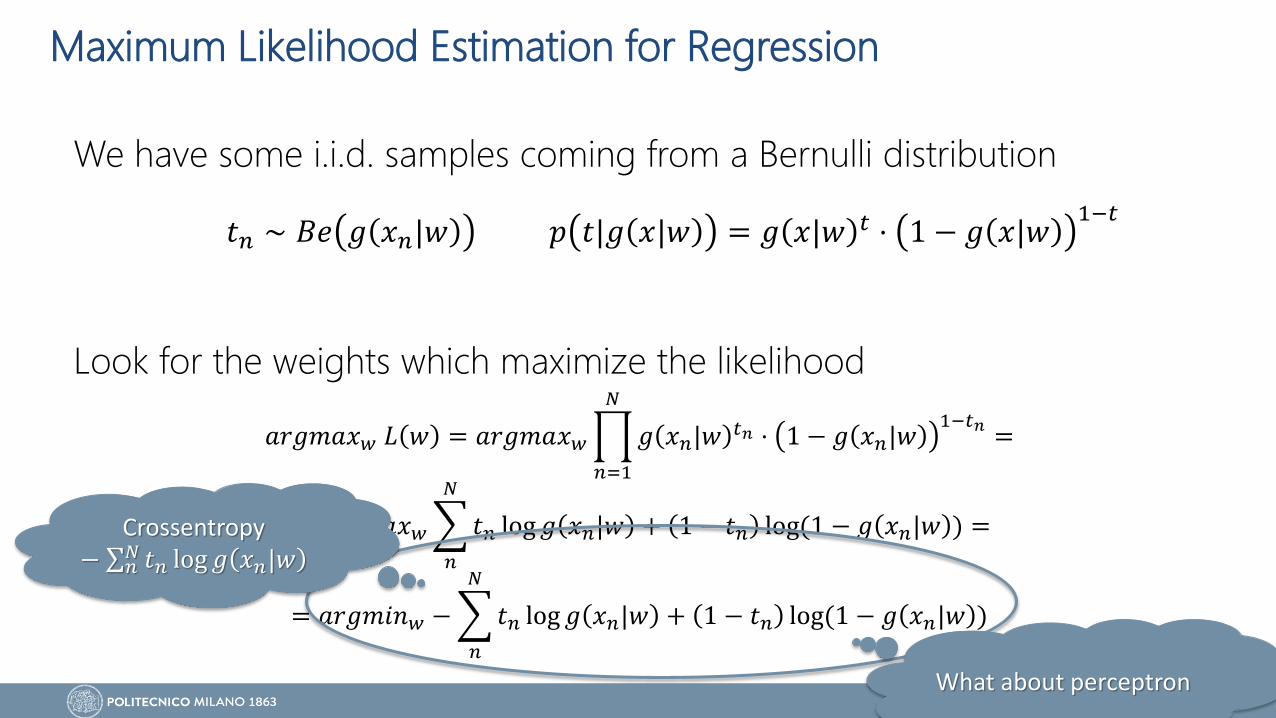
Maximum Likelihood Estimation for Regression
We have some i.i.d. samples coming from a Bernulli distribution
Look for the weights which maximize the likelihood
𝑝 𝑡|𝑔 𝑥|𝑤 = 𝑔 𝑥|𝑤 𝑡 ⋅ 1 − 𝑔 𝑥|𝑤1−𝑡
𝑎𝑟𝑔𝑚𝑎𝑥𝑤 𝐿 𝑤 = 𝑎𝑟𝑔𝑚𝑎𝑥𝑤
𝑛=1
𝑁
𝑔 𝑥𝑛|𝑤 𝑡𝑛 ⋅ 1 − 𝑔 𝑥𝑛|𝑤1−𝑡𝑛
=
= 𝑎𝑟𝑔𝑚𝑎𝑥𝑤
𝑛
𝑁
𝑡𝑛 log 𝑔 𝑥𝑛|𝑤 + 1 − 𝑡𝑛 log(1 − 𝑔 𝑥𝑛|𝑤 ) =
= 𝑎𝑟𝑔𝑚𝑖𝑛𝑤 −
𝑛
𝑁
𝑡𝑛 log 𝑔 𝑥𝑛|𝑤 + 1 − 𝑡𝑛 log(1 − 𝑔 𝑥𝑛|𝑤 )
𝑡𝑛 ∼ 𝐵𝑒 𝑔 𝑥𝑛|𝑤
Crossentropy− 𝑛
𝑁 𝑡𝑛 log 𝑔 𝑥𝑛|𝑤
What about perceptron
48
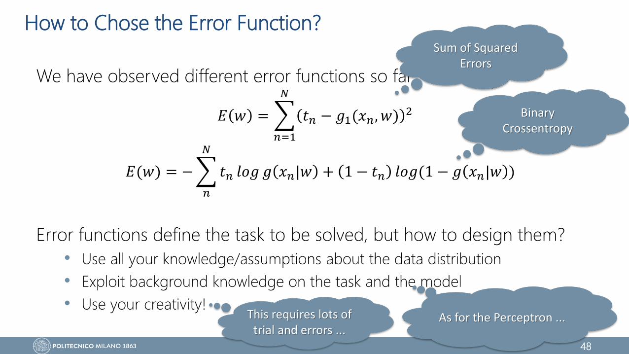
How to Chose the Error Function?
We have observed different error functions so far
Error functions define the task to be solved, but how to design them?
• Use all your knowledge/assumptions about the data distribution
• Exploit background knowledge on the task and the model
• Use your creativity!This requires lots of
trial and errors ...
𝐸 𝑤 =
𝑛=1
𝑁
𝑡𝑛 − 𝑔1(𝑥𝑛, 𝑤) 2
Sum of Squared Errors
As for the Perceptron ...
𝐸(𝑤) = −
𝑛
𝑁
𝑡𝑛 𝑙𝑜𝑔 𝑔 𝑥𝑛|𝑤 + 1 − 𝑡𝑛 𝑙𝑜𝑔(1 − 𝑔 𝑥𝑛|𝑤 )
Binary Crossentropy
49
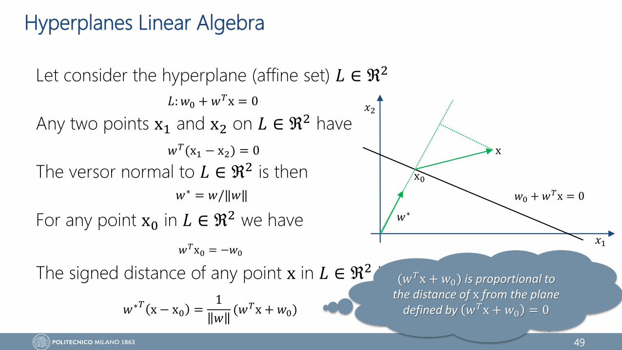
Hyperplanes Linear Algebra
Let consider the hyperplane (affine set) 𝐿 ∈ ℜ2
Any two points x1 and x2 on 𝐿 ∈ ℜ2 have
The versor normal to 𝐿 ∈ ℜ2 is then
For any point x0 in 𝐿 ∈ ℜ2 we have
The signed distance of any point x in 𝐿 ∈ ℜ2 is defined by
𝑥1
𝑤0 + 𝑤𝑇x = 0
𝑥2
x
x0
𝑤∗
𝐿: 𝑤0 + 𝑤𝑇x = 0
𝑤𝑇(x1 − x2) = 0
𝑤∗ = 𝑤/‖𝑤‖
𝑤∗𝑇 x − x0 =1
𝑤(𝑤𝑇x + 𝑤0)
𝑤𝑇x0 = −𝑤0
(𝑤𝑇x + 𝑤0) is proportional to the distance of x from the plane
defined by 𝑤𝑇x + 𝑤0 = 0
50
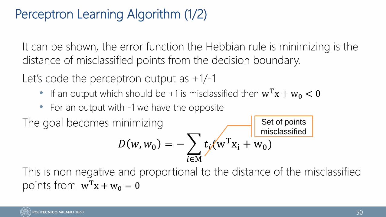
It can be shown, the error function the Hebbian rule is minimizing is the
distance of misclassified points from the decision boundary.
Let’s code the perceptron output as +1/-1
• If an output which should be +1 is misclassified then wTx + w0 < 0
• For an output with -1 we have the opposite
The goal becomes minimizing
𝐷 𝑤,𝑤0 = −
𝑖∈M
𝑡𝑖(wTxi + w0)
This is non negative and proportional to the distance of the misclassified
points from
Set of points
misclassified
Perceptron Learning Algorithm (1/2)
wTx + w0 = 0
51
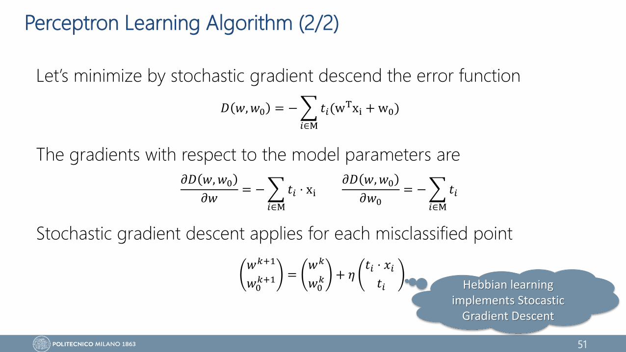
Let’s minimize by stochastic gradient descend the error function
The gradients with respect to the model parameters are
Stochastic gradient descent applies for each misclassified point
Perceptron Learning Algorithm (2/2)
𝐷 𝑤, 𝑤0 = −
𝑖∈M
𝑡𝑖(wTxi + w0)
𝜕𝐷 𝑤, 𝑤0
𝜕𝑤= −
𝑖∈M
𝑡𝑖 ⋅ xi
𝜕𝐷 𝑤, 𝑤0
𝜕𝑤0= −
𝑖∈M
𝑡𝑖
𝑤𝑘+1
𝑤0𝑘+1 =
𝑤𝑘
𝑤0𝑘 + 𝜂
𝑡𝑖 ⋅ 𝑥𝑖
𝑡𝑖 Hebbian learning implements Stocastic
Gradient Descent
Recommended