* Corresponding author, tel: +234 – 806 – 435 – 0200
ASSESSMENT OF TRAFFIC FLOW ON ENUGU HIGHWAYS USING SPEED
DENSITY REGRESSION COEFFICIENT
H. K. Ugwuanyi1,*, F. O. Okafor2 and J. C. Ezeokonkwo3 1, DEPARTMENT OF CIVIL ENGINEERING, MICHAEL OKPARA UNIV. OF AGRICULTURE, UMUDIKE, ABIA STATE, NIGERIA
2, 3, DEPARTMENT OF CIVIL ENGINEERING, UNIVERSITY OF NIGERIA, NSUKKA, ENUGU STATE, NIGERIA
E-mail addresses: 1 [email protected], 2 [email protected], 3 [email protected]
ABSTRACT
In an attempt to estimate the operating speeds and volume of traffic on highway lanes as a function of predicted
demands, speed-density models were estimated using data from highway sites. Speed, flow and volume are the most
important elements of the traffic flow. In this study, the speed-density regression models are compared using five
highways in relation to their correlation coefficient based on the daily traffic flow data obtained from the roads. The
traffic flow data were collected by hourly traffic count on each road. The coefficient of correlation (R) proved to have the
best fit with a higher confidence and less variation for a two-lane highway than a one-lane highway. The space-mean
speed (u) and density (k) relationship for the two-lane highways are; u , and
u whereas the space-mean speed (u) and density (k) relationship for the one-lane highways are; u =
respectively. This research provides practical application for speed estimation,
construction, maintenance and optimization of the highways using the speed-density models which will enhance traffic
monitoring, traffic control management, traffic forecasting and model calibration.
Keywords: speed, density, flow, traffic count, correlation coefficient.
1. INTRODUCTION
Annual Average Daily Traffic, (AADT), is a measure used
primarily in transportation planning and transportation
engineering. Traditionally, it is the total volume of
vehicle traffic of a highway or road for a year divided by
365 days. In 1992, American Association of State
Highways and Transport Officials (AASHTO) released the
AASHTO Guidelines for Traffic Data Programs which
identified a way to produce an AADT without seasonal or
day-of-week biases by creating an "average of averages”
[1]. AADT is a useful and simple measurement of how
busy the road is. Newer advances from traffic data
providers are now providing AADT by side of the road,
by day of week and by time of day. The presence of
several hourly-congested highways forces researchers to
better understand freeway operations under congested
condition. The intelligent vehicle-highway system (like
speed enforcement) programs will be able to function
effectively if traffic behaviours under all conditions are
modeled accurately [2].
Traffic flow in engineering is the study of interaction
between vehicles, commuters and infrastructure
(including the highways, signage and traffic control
devices) with the aim of understanding and developing
an optimal road network with efficient movement of
traffic and minimal traffic congestion problems. The
existing transportation facility which was originally
designed and constructed to be adequate for the past
traffic volume becomes practically inadequate to handle
the present day traffic demand, resulting to an inevitable
tremendous traffic congestion along the highway [3].
Most highways in Nigeria were designed without taking
into consideration the daily traffic volume of the highway
and the speed limits at necessary points along the
highway. The tendency of the drivers to exceed the road
design speed limits become prevalent leading to traffic
accidents and conflicts. Thus, there is the need for
road/highway designers to use a valid model equation to
help calibrate the speed limits in relation to the traffic
density obtained at the section of the road.
The term traffic flow and volume are used
interchangeably to define the number of vehicles that ply
a particular road network at a given period of time.
Queuing and delay occur in all congested situations;
therefore a study on flow, speed and density on the roads
would be relevant and necessitates a proper design of
their intersection.
Nigerian Journal of Technology (NIJOTECH)
Vol. 36, No. 3, July 2017, pp. 749 – 757
Copyright© Faculty of Engineering, University of Nigeria, Nsukka, Print ISSN: 0331-8443, Electronic ISSN: 2467-8821
www.nijotech.com http://dx.doi.org/10.4314/njt.v36i3.13
ASSESSMENT OF TRAFFIC FLOW ON ENUGU HIGHWAYS USING SPEED DENSITY REGRESSION COEFFICIENT, H. K. Ugwuanyi, et al
Nigerian Journal of Technology Vol. 36, No. 3, July 2017 750
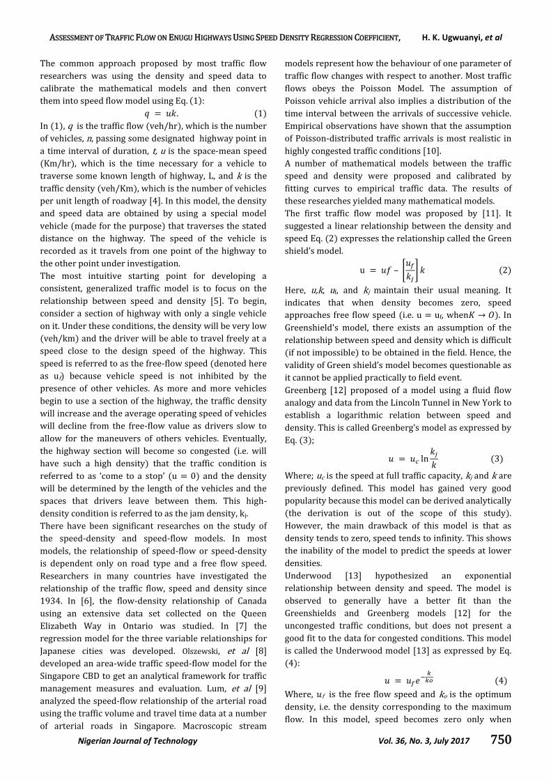
The common approach proposed by most traffic flow
researchers was using the density and speed data to
calibrate the mathematical models and then convert
them into speed flow model using Eq ( )
( )
In (1), q is the traffic flow (veh/hr), which is the number
of vehicles, n, passing some designated highway point in
a time interval of duration, t, u is the space-mean speed
(Km/hr), which is the time necessary for a vehicle to
traverse some known length of highway, L, and k is the
traffic density (veh/Km), which is the number of vehicles
per unit length of roadway [4]. In this model, the density
and speed data are obtained by using a special model
vehicle (made for the purpose) that traverses the stated
distance on the highway. The speed of the vehicle is
recorded as it travels from one point of the highway to
the other point under investigation.
The most intuitive starting point for developing a
consistent, generalized traffic model is to focus on the
relationship between speed and density [5]. To begin,
consider a section of highway with only a single vehicle
on it. Under these conditions, the density will be very low
(veh/km) and the driver will be able to travel freely at a
speed close to the design speed of the highway. This
speed is referred to as the free-flow speed (denoted here
as uf) because vehicle speed is not inhibited by the
presence of other vehicles. As more and more vehicles
begin to use a section of the highway, the traffic density
will increase and the average operating speed of vehicles
will decline from the free-flow value as drivers slow to
allow for the maneuvers of others vehicles. Eventually,
the highway section will become so congested (i.e. will
have such a high density) that the traffic condition is
referred to as ‘come to a stop’ (u 0) and the density
will be determined by the length of the vehicles and the
spaces that drivers leave between them. This high-
density condition is referred to as the jam density, kj.
There have been significant researches on the study of
the speed-density and speed-flow models. In most
models, the relationship of speed-flow or speed-density
is dependent only on road type and a free flow speed.
Researchers in many countries have investigated the
relationship of the traffic flow, speed and density since
1934. In [6], the flow-density relationship of Canada
using an extensive data set collected on the Queen
Elizabeth Way in Ontario was studied. In [7] the
regression model for the three variable relationships for
Japanese cities was developed. Olszewski, et al [8]
developed an area-wide traffic speed-flow model for the
Singapore CBD to get an analytical framework for traffic
management measures and evaluation. Lum, et al [9]
analyzed the speed-flow relationship of the arterial road
using the traffic volume and travel time data at a number
of arterial roads in Singapore. Macroscopic stream
models represent how the behaviour of one parameter of
traffic flow changes with respect to another. Most traffic
flows obeys the Poisson Model. The assumption of
Poisson vehicle arrival also implies a distribution of the
time interval between the arrivals of successive vehicle.
Empirical observations have shown that the assumption
of Poisson-distributed traffic arrivals is most realistic in
highly congested traffic conditions [10].
A number of mathematical models between the traffic
speed and density were proposed and calibrated by
fitting curves to empirical traffic data. The results of
these researches yielded many mathematical models.
The first traffic flow model was proposed by [11]. It
suggested a linear relationship between the density and
speed Eq. (2) expresses the relationship called the Green
shield’s model.
u [
] ( )
Here, u,k, uf, and kj maintain their usual meaning. It
indicates that when density becomes zero, speed
approaches free flow speed (i.e. u = uf, when ). In
Greenshield's model, there exists an assumption of the
relationship between speed and density which is difficult
(if not impossible) to be obtained in the field. Hence, the
validity of Green shield’s model becomes questionable as
it cannot be applied practically to field event.
Greenberg [12] proposed of a model using a fluid flow
analogy and data from the Lincoln Tunnel in New York to
establish a logarithmic relation between speed and
density This is called Greenberg’s model as expressed by
Eq. (3);
ln
( )
Where; uc is the speed at full traffic capacity, kj and k are
previously defined. This model has gained very good
popularity because this model can be derived analytically
(the derivation is out of the scope of this study).
However, the main drawback of this model is that as
density tends to zero, speed tends to infinity. This shows
the inability of the model to predict the speeds at lower
densities.
Underwood [13] hypothesized an exponential
relationship between density and speed. The model is
observed to generally have a better fit than the
Greenshields and Greenberg models [12] for the
uncongested traffic conditions, but does not present a
good fit to the data for congested conditions. This model
is called the Underwood model [13] as expressed by Eq.
(4):
( )
Where, f is the free flow speed and ko is the optimum
density, i.e. the density corresponding to the maximum
flow. In this model, speed becomes zero only when

ASSESSMENT OF TRAFFIC FLOW ON ENUGU HIGHWAYS USING SPEED DENSITY REGRESSION COEFFICIENT, H. K. Ugwuanyi, et al
Nigerian Journal of Technology Vol. 36, No. 3, July 2017 751
density reaches infinity which is the drawback of this
model. Hence this cannot be used for predicting speeds
at high densities.
Drake, et al [14] studied the various macroscopic traffic
models postulated at that time and did not find any of
them statistically significant. In developing his model, he
estimated the density from speed and flow data, fitted
the speed versus density function and transformed the
speed versus density function to a speed versus flow
function. The formulation of the [14] model is expressed
by Eq. (5) and is called the Drake model:
exp [
(
) ] ( )
Where, kc is the density at capacity. His model generally
yields a better fit than the above three models for
uncongested conditions.
From the review above, it is obvious that most
researchers focused on the character of the network
roads, using traffic data generated by electronic counting
machines without actually taking physical field traffic
record, and lacking of comparisons of different road
configurations. The researches were carried out mostly
in the western world where road failures are rare and
observation of traffic laws is held esteem, unlike in
Nigeria that has a lot of the failed section of the highways
and little or no observation to traffic laws. Hence, the
postulated models above may be non-functional to
Nigerian highways. In addition, many of the models were
calibrated by using assumed and estimated values of the
traffic data which is non-practical to field phenomenon.
Some of them applied unattainable values to the traffic
data, thus invalidating the postulated model.
This research paper is to compare the speed-density
classical linear model to calibrate functional relationship
based on the field recorded daily traffic data by a manual
traffic count obtained from five (5) highways (with
distinct number of lanes) in Enugu, Enugu State. So they
represent two different kinds of roads being assessed by
various traffic compositions.
2. METHODOLOGY AND DATA COLLECTION
2.1. The Study Area.
The data in this study were obtained from five (5)
highways in Enugu, Enugu Sate. The roads include:
1. Enugu 9TH Mile Expressway (E9E)
2. Enugu Abakaliki Expressway (EAE)
3. Enugu Port Harcourt Expressway (EPE)
4. 9th Mile Onitsha Expressway (9OE)
5. 9th Mile Oji-River Expressway (9ORE)
The locations of the two roads to be used for the full
analysis are shown in the Figures 1 and 2 with a
highlighter. These two roads are the representatives of
the rest of the highways. Figure 1 is an aerial map of the
communities close to the Enugu-9th Mile Expressway,
with the road shown with a highlighter. The arrows
pointing in both directions indicate that the road is a 2-
way highway. E9E has 2 lanes with the carriage width of
10m average. It originated from New Market junction
and goes through Gulf estate and continued its course to
Onitsha. This highway is notorious for skidding away of
heavy lorries and trailers/tanker, also head-on vehicular
collision.
Figure 2 shows the aerial map of the towns surrounding
Enugu-Abakaliki Expressway, with the road under study
shown with dark highlighter indicating a two-way
direction movement.
EAE has one lane of average width of 9.8m. It originated
from Airport Road junction, goes through PRODA
Headquarters and continued to Abakaliki.
Figure 1: Map showing Enugu 9th Mile Expressway
Figure 2: Map showing Enugu Abakaliki
Expressway
2.2. Method of Data Collection
Regression analysis was conducted based on the
collected data by the road manual hourly traffic counters
on the two highways. Fourteen (14) human recorders
(counters) were stationed at Point A and Point B of 1km
distance of separation, seven (7) counters at one point
on the road side, each counter recording one type of
traffic composition. Each of the recorders was replaced
by other recorders to avoid over-labour and fatigue.
Then at the end of every hourly traffic record, the
average of the volume of traffic composition at Points A
and B is taken as the hourly traffic volume. The traffic

ASSESSMENT OF TRAFFIC FLOW ON ENUGU HIGHWAYS USING SPEED DENSITY REGRESSION COEFFICIENT, H. K. Ugwuanyi, et al
Nigerian Journal of Technology Vol. 36, No. 3, July 2017 752
count can be diagrammatically and mathematically
expressed in the Figure 3.
Hourly daily traffic, Hd is expressed by Eq. (6) as follows:
( )
The time of record transition is taken to be one minutes
of average lagging. We have seven traffic composition in
consideration; 1. Motorcycle, 2. Tricycle, 3. Pickup/cars,
4. Mini buses, 5. Luxurious buses, 6. Lorry/trucks, 7.
Tankers/trailers.
The hourly traffic count was done for seven consecutive
days after which the summary of the count was recorded.
Table 1 and 2 show the summary of the hourly traffic
count collected from 07:00hrs 19:00hrs (from Enugu
9th Mile Expressway and Enugu Abakaliki Expressway
respectively) for a period of seven consecutive days
using Eq. (6) [15].
2.3. Model Formulation and Calibration
Using a linear relationship between space-mean speed
and density, the model equation can be formulated as
stated in Eqs. (7 10) respectively. Let
( )
Where: y is the speed (u), x is the density (k), R is the
correlation coefficient, a, b is the constants to be
determined.,
∑ (∑ )(∑ )
√[ (∑ ) (∑ )
)] √[ (∑ ) (∑ )
)]
( )
n ∑ x y
∑ x ∑ y
n ∑ x ( ∑ x
)
( )
( 0)
Where and are the average values of y and x
respectively
H I G H W A Y
Point A (7counters) To-direction Point B (7counters)
L = 1km
Figure 3: Diagrammatic representation of the traffic counting positions
Table 1: Traffic count done along Enugu 9th Mile Highway in accordance with the Road Safety Standard by the Federal
Road Safety Corps, Enugu State Command, 2015. TRAFFIC COUNT TEMPLATE (SUMMARY SHEET)
COMMAND- RS9.1 ENUGU SECTOR COMMAND
DIRECTION INDICATORS: TO ROUTE:ENU-9THMILE
TIME INTERVAL
DAY ONE 21/09/2015
DAY TWO 22/09/2015
DAY THREE 23/09/2015
DAY FOUR 24/09/2015
DAY FIVE 25/09/2015
DAY SIX 26/09/2015
DAY SEVEN 27/09/15
TOTAL
0700-0800HRS
459 297 291 252 297 320 162 2078
0801-0900HRS
540 556 353 290 336 365 189 2629
0901-1000HRS
358 424 455 312 370 380 189 2488
1001-1100HRS
302 286 513 345 448 408 194 2496
1101-1200HRS
272 251 453 339 459 527 179 2480
1201-1300HRS
224 285 449 351 476 508 259 2520
1301-1400HRS
259 334 451 414 495 450 297 2700
1401-1500HRS
292 321 424 472 525 508 281 2823
1501-1600HRS
304 332 436 493 534 544 302 2945
1601-1700HRS
362 367 533 496 549 560 337 3204
1701-1800HRS
382 385 593 513 396 532 351 3152
1801-1900HRS
354 328 473 524 351 380 235 2645
TOTAL 4108 4166 5424 4801 5236 5482 2975 32160

ASSESSMENT OF TRAFFIC FLOW ON ENUGU HIGHWAYS USING SPEED DENSITY REGRESSION COEFFICIENT, H. K. Ugwuanyi, et al
Nigerian Journal of Technology Vol. 36, No. 3, July 2017 753
Table 2: Traffic count done along Enugu Abakaliki Highway in accordance with the Road Safety Standard by the
Federal Road Safety Corps, Enugu State Command, 2015.
TRAFFIC COUNT TEMPLATE (SUMMARY SHEET)
COMMAND- RS9.1 ENUGU SECTOR COMMAND
DIRECTION INDICATORS: TO-DIRECTION ROUTE: ENUGU - ABAKALIKI
TIME INTERVAL
DAY ONE 23/12/2015
DAY TWO 24/12/2015
DAY THREE 25/12/2015
DAY FOUR 26/12/2015
DAY FIVE 27/12/2015
DAY SIX 28/12/2015
DAY SEVEN 29/12/2015
TOTAL
0700-0800HRS
338 439 187 197 161 244 188 1754
0801-0900HRS
367 519 272 228 184 258 202 2030
0901-1000HRS
418 546 310 173 203 260 253 2163
1001-1100HRS
447 577 252 227 235 277 206 2221
1101-1200HRS
490 624 253 228 246 301 200 2342
1201-1300HRS
552 714 253 204 272 307 208 2510
1301-1400HRS
627 681 331 225 267 261 237 2629
1401-1500HRS
628 693 419 222 271 235 240 2708
1501-1600HRS
524 692 451 228 286 218 271 2670
1601-1700HRS
661 699 448 243 286 213 287 2837
1701-1800HRS
588 814 431 254 246 220 231 2784
1801-1900HRS
553 681 349 194 234 130 189 2330
TOTAL 6193 7679 3956 2623 2891 2924 2712 22785
2.4 Calculation of the Flow, Speed and Density.
Traffic Flow, q, is simply defined as the number of
vehicles, n, passing some designated highway point in a
time interval of duration, t, as expressed by Eq. (11) as:
( )
Here q is the traffic flow (veh/hr), n is the number of
vehicles, t is the time interval (hr). Space Mean Speed,
u, is the time necessary for a vehicle to traverse some
known length of highway, L. If all vehicle speeds are
measured over the same length of highway (L = L1 = L2
… Ln), then u is expressed as:
u
(
(
)∑
( )
⁄
)
( )
where, L = length of highway under study (Km),ti = time
interval of ith vehicle (hr).
Traffic Density (k) in veh/km is defined by Eq. (13) as:
( )
As usual, n and L maintain their usual meanings and
units. In this paper, the Microsoft Excel Worksheet from
Microsoft Office 2007® was employed in the calculation
to aid in handling of large data and eliminates
computation errors for computation of space-mean
speed, u, length, L of highway under study = 1km, Time
interval, (t) = 1hr for the first sample record of traffic
and 0.9833hr for the rest of the sample.
3. RESULTS AND DISCUSSION
3.1. Enugu 9th Mile Expressway (E9E).
Using Day 6 (26-9-2015) for the computation, because it
has the highest volume of daily traffic, n = 5482 vehicles
Computing in tabular form by using Microsoft Excel
spread sheet from Table 1from Eqs.11, 12 and 13
respectively the traffic flow, q, speed, u and density, k can
be calculated on hourly basis as can be seen in Table 3
(for Enugu 9th Mile) and Table 4 (for Enugu
Abakaliki).
3.2 Computation of Coefficient of Regression, (r or R).
Denoting speed (u) = y, density (k) = x, n = number of
hourly sample (n = 12). From Table 4, the values of the
space-mean speed and density are imported from Table
3 above. Using statistical equation to create another table
for the coefficient of correlation in an Excel Worksheet,
the value of coefficient of correlation, R can be found.
ASSESSMENT OF TRAFFIC FLOW ON ENUGU HIGHWAYS USING SPEED DENSITY REGRESSION COEFFICIENT, H. K. Ugwuanyi, et al
Nigerian Journal of Technology Vol. 36, No. 3, July 2017 754
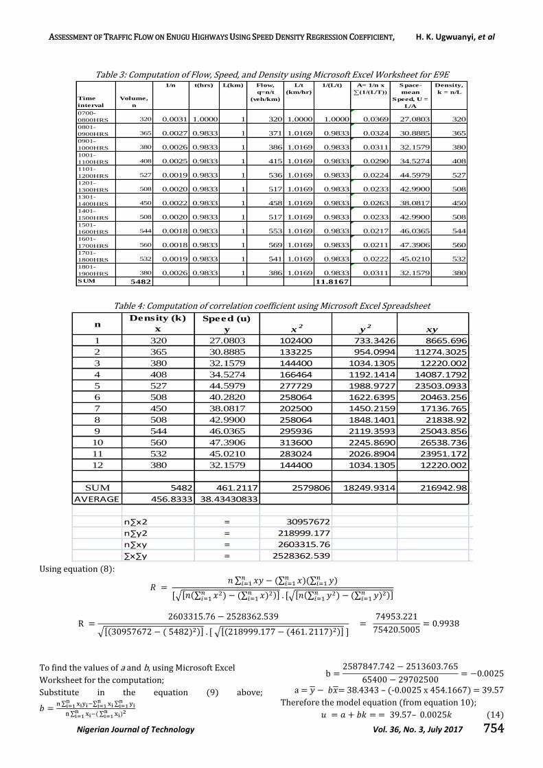
Table 3: Computation of Flow, Speed, and Density using Microsoft Excel Worksheet for E9E
Time
interval
Volume,
n
1/n t(hrs) L(km) Flow,
q=n/t
(veh/km)
L/t
(km/hr)
1/(L/t) A= 1/n x
∑(1/(L/T))
Space-
mean
Speed, U =
L/A
Density,
k = n/L
0700-
0800HRS 320 0.0031 1.0000 1 320 1.0000 1.0000 0.0369 27.0803 3200801-
0900HRS 365 0.0027 0.9833 1 371 1.0169 0.9833 0.0324 30.8885 3650901-
1000HRS 380 0.0026 0.9833 1 386 1.0169 0.9833 0.0311 32.1579 3801001-
1100HRS 408 0.0025 0.9833 1 415 1.0169 0.9833 0.0290 34.5274 4081101-
1200HRS 527 0.0019 0.9833 1 536 1.0169 0.9833 0.0224 44.5979 5271201-
1300HRS 508 0.0020 0.9833 1 517 1.0169 0.9833 0.0233 42.9900 5081301-
1400HRS 450 0.0022 0.9833 1 458 1.0169 0.9833 0.0263 38.0817 4501401-
1500HRS 508 0.0020 0.9833 1 517 1.0169 0.9833 0.0233 42.9900 5081501-
1600HRS 544 0.0018 0.9833 1 553 1.0169 0.9833 0.0217 46.0365 5441601-
1700HRS 560 0.0018 0.9833 1 569 1.0169 0.9833 0.0211 47.3906 5601701-
1800HRS 532 0.0019 0.9833 1 541 1.0169 0.9833 0.0222 45.0210 5321801-
1900HRS 380 0.0026 0.9833 1 386 1.0169 0.9833 0.0311 32.1579 380SUM 5482 11.8167
Table 4: Computation of correlation coefficient using Microsoft Excel Spreadsheet
nDensity (k)
x
Speed (u)
y x2
y2
xy
1 320 27.0803 102400 733.3426 8665.696
2 365 30.8885 133225 954.0994 11274.3025
3 380 32.1579 144400 1034.1305 12220.002
4 408 34.5274 166464 1192.1414 14087.1792
5 527 44.5979 277729 1988.9727 23503.0933
6 508 40.2820 258064 1622.6395 20463.256
7 450 38.0817 202500 1450.2159 17136.765
8 508 42.9900 258064 1848.1401 21838.92
9 544 46.0365 295936 2119.3593 25043.856
10 560 47.3906 313600 2245.8690 26538.736
11 532 45.0210 283024 2026.8904 23951.172
12 380 32.1579 144400 1034.1305 12220.002
SUM 5482 461.2117 2579806 18249.9314 216942.98
AVERAGE 456.8333 38.43430833
n∑x2 = 30957672
n∑y2 = 218999.177
n∑xy = 2603315.76
∑x∑y = 2528362.539 Using equation (8):
∑ (∑ )(∑ )
√ (∑ ) (∑ )
)] √ (∑ ) (∑ )
)]
0
√ ( 0 ( ) )] √ ( ( ) )] ]
0 00 0
To find the values of a and b, using Microsoft Excel
Worksheet for the computation;
Substitute in the equation (9) above;
∑
∑ ∑
∑ ( ∑
)
b 0
00 0 00 0 00
a = = 38.4343 (-0.0025 x 454.1667) = 39.57
Therefore the model equation (from equation 10);
0 00 ( )

ASSESSMENT OF TRAFFIC FLOW ON ENUGU HIGHWAYS USING SPEED DENSITY REGRESSION COEFFICIENT, H. K. Ugwuanyi, et al
Nigerian Journal of Technology Vol. 36, No. 3, July 2017 755
This value of R = 0.9938shows a best fit of the data
analysis and thus has a very high confidence and less
variation of the traffic data. The Figure 4.1 shows the
graph of space-mean speed against density for Enugu
9th Mile Expressway. From the graph, as the density
increases, the speed decreases because drivers slow
down to allow for maneuvers of other vehicles.
Consequently, when where there are very few vehicles
along the highway, the density becomes very low and the
drivers will be able to travel freely to a maximum speed.
This maximum speed is referred to as free flow speed, uf.
From Figure 4.1 uf = 39.57km/hr when k = 0. This
maximum value of speed is the design speed at that
particular highway section.
3.2. Enugu Abakaliki Expressway.
Using Day 2 (24-12-2015) for the computation, because
it has the highest volume of daily traffic. As explained in
section 3.1, the flow, space-mean speed and density can
be calculated using the formulae in equations 11, 12 and
13 respectively. Table 5 shows the values of the traffic
parameters as computed using Microsoft Excel
Worksheet® 2007.
Fig. 4: Plot of Space-mean Speed versus Traffic Density
for E9E
3.3 Computation of Coefficient of correlation, (r or R).
Denoting speed (u) = y, density (k) = x, n = number of
hourly sample (n = 12). Table 6 shows the statistical
values of the computation for calculation of coefficient of
correlation, R. Using equation (8) to calculate R.
Table 5: Analysis of Flow, Speed, Density using Microsoft Excel Worksheet for EAE Time
interval
Volume,
n
1/n t(hrs) L(km) Flow,
q=n/t
L/t 1/(L/t) A= 1/n x
∑(1/(L/T))
Speed, U =
L/A
Density, k
= n/L
0700-
0800HRS
439
0.0023 1.0000 1 439 1.0000 1.0000 0.0269 37.1508 439
0801-
0900HRS
519
0.0019 0.9833 1 528 1.0169 0.9833 0.0228 43.9209 519
0901-
1000HRS
546
0.0018 0.9833 1 555 1.0169 0.9833 0.0216 46.2058 546
1001-
1100HRS
577
0.0017 0.9833 1 587 1.0169 0.9833 0.0205 48.8292 577
1101-
1200HRS
624
0.0016 0.9833 1 635 1.0169 0.9833 0.0189 52.8066 624
1201-
1300HRS
654
0.0015 0.9833 1 665 1.0169 0.9833 0.0181 55.3454 654
1301-
1400HRS
681
0.0015 0.9833 1 693 1.0169 0.9833 0.0174 57.6303 681
1401-
1500HRS
693
0.0014 0.9833 1 705 1.0169 0.9833 0.0171 58.6458 693
1501-
1600HRS
692
0.0014 0.9833 1 704 1.0169 0.9833 0.0171 58.5612 692
1601-
1700HRS
699
0.0014 0.9833 1 711 1.0169 0.9833 0.0169 59.1536 699
1701-
1800HRS
685
0.0015 0.9833 1 697 1.0169 0.9833 0.0173 57.9688 685
1801-
1900HRS
870
0.0011 0.9833 1 885 1.0169 0.9833 0.0136 73.6246 870
SUM 7679 11.8167
Table 6: Computation of regression coefficient using Microsoft Excel Spreadsheet
n
DENSITY(k)
x
SPEED(u)
y x2
y2
xy
1 439 37.1508 192721 1380.1819 16309.2012
2 519 43.9209 269361 1929.0455 22794.9471
3 546 46.2058 298116 2134.9760 25228.3668
4 577 48.8292 332929 2384.2908 28174.4484
5 624 52.8066 389376 2788.5370 32951.3184
6 654 55.3454 427716 3063.1133 36195.8916
7 681 57.6303 463761 3321.2515 39246.2343
8 693 58.6458 480249 3439.3299 40641.5394
9 692 58.5612 478864 3429.4141 40524.3504
10 699 59.1536 488601 3499.1484 41348.3664
11 685 57.9688 469225 3360.3818 39708.628
12 870 57.6303 756900 3321.2515 50138.361
SUM 7679 633.8487 5047819 34050.9216 413261.653
AVERAGE 639.9167 52.820725
( ) ( )
[√ ( 0 ) ) ] ] [√[ ( 0 0 ) ( ) ]]]
0 0

ASSESSMENT OF TRAFFIC FLOW ON ENUGU HIGHWAYS USING SPEED DENSITY REGRESSION COEFFICIENT, H. K. Ugwuanyi, et al
Nigerian Journal of Technology Vol. 36, No. 3, July 2017 756
To find a and b using equations (8) and (9), substitute in
equation (9),
0 0 00
52.8207 ( 0 00 x 639.9167) =
Therefore the model equation is;
0 00 ( )
Figure 5 shows the graph of space-mean speed against
density for Enugu Abakaliki Expressway. From the
graph, it can be observed that the there is a little
variation in the traffic data. As the density increases, the
speed decreases because the drivers allow for the safe
maneuver of other speeding vehicles. The free flow speed
when the density is zero is uf = 47.13Km/hr. this is the
design speed of the highway which must not be exceeded
at the section of the highway. At a certain point in the
graph, the speed drops drastically due to the influx of
vehicles trying to pass the highway section at the same
time.
From the calibrated equation (14), u = 38.38 0.0025k
for E9E, and equation (15), u = 0 00 for EAE,
as the traffic density increases, the space-mean speed
decreases, and vice versa. It shows that when there are
few vehicles on a highway, the vehicles tend to maximize
the design speed of the road which is limited to a certain
value. This is in contrast to the findings of other
researchers which asserted that at a very low density,
the speed tends to infinity which is not realistic in the
field. The limitation of speed level to a maximum value
rather than infinity is as a result of the effect of field
phenomena like merging/diverging traffic, breakdown of
vehicle that suddenly comes to a stop, traffic joining the
highway from a minor road, commercial
vehicles/tricycles braking to pick or drop passengers and
so on. Table 7 shows traffic data differences of the two
roads under study, indicating the jam density (kj) and the
free flow speed (uf)
The quantity R, called the linear correlation coefficient,
measures the strength and the direction of the linear
relationship between space-mean speed and traffic
density. Since the correlation is greater than 0.8, it is
generally described as strong. The coefficient of
determination, R 2, gives the proportion of the variance
(fluctuation) of space-mean speed that is predictable
from the density. The coefficient of determination
represents the percent of the data that is the closest to
the line of best fit. For E9E, R2 = 0.9876, means that
98.76% of the total variation in speed can be explained
by the linear relationship between density and speed (as
described by the regression equation). The other 1.24%
of the total variation in speed indicates the
diverted/merged traffic after/before being counted at
one point of traffic counting position. For EAE, R2 =
0.7662, means that 76.62% of the total variation in speed
can be explained by the linear relationship between
density and speed. The other 23.38% of the total
variation in speed indicates the diverted/merged traffic
after/before being counted at one point of traffic
counting position. This is an indication that more
vehicles diverge to or merge from other service roads
than on the E9E.
It was also observed that the Enugu 9th Mile
Expressway has a higher value of R, (best fit) and high
confidence but has a lower value of the speed density
relationship than the Enugu Abakaliki Expressway.
This is because of the differences in the structure and the
traffic composition of the two highways.
Figure 5: Plot of Space-mean Speed (u) against Traffic
Density (k) for EAE
Table 7: Traffic data values for E9E and EAE
Name of Road
Number of Lanes
Correlation Coefficient, R
Coefficient Of Determination,R2
Model Equation Jam Density, (veh/km) kj
Free Flow Speed, (Km/hr)
uf
E9E 2 0.9938 0.9878 u = 38.32 - 0.0025k 15,328 38.32 EAE 1 0.8753 0.7662 u= 53.84 - 0.0016k 33,650 53.84

ASSESSMENT OF TRAFFIC FLOW ON ENUGU HIGHWAYS USING SPEED DENSITY REGRESSION COEFFICIENT, H. K. Ugwuanyi, et al
Nigerian Journal of Technology Vol. 36, No. 3, July 2017 757
Table 8: Traffic data values for EPE, 9OE, and 9ORE
Name of Road
Number of Lanes
Correlation Coefficient, R
Coefficient of Determination,R2
Model Equation Jam Density, (veh/km) kj
Free Flow Speed, (Km/hr) uf
EPE 2 0.9818 0.9757 0 0 5,867 58.67
9OE 2 0.9746 0.9498 0 00 16,575 33.15
9ORE 1 0.8651 0.7483 0 00 9,920 29.76
E9E is a two-lane highway with various dilapidated points
and conflicts/accident prone zones, comprising mostly of
heavy duty trucks and lorries, which as a result of the
nature of the road, travel at a lower speed. This is evidence
to the reduced value of the space-mean speed of traffic as
many vehicles try to maneuver from one lane to the other.
EAE is a one-lane highway with little number of pot holes
and conflict zones. The value of R is lower because of
frequent stopping, diverging and merging (from other
minor roads) of commercial vehicle passing through a
section of the highway to serve their passengers. It was also
observed that the hourly traffic flow is higher on EAE than
on E9E as can be seen in Table 7. This is due to some road
users having alternatives to the use of E9E.
Similar work done for Enugu Port Harcourt Expressway
(EPE), 9TH Mile Onitsha Expressway (9OE), and 9TH Mile
Oji River Expressway (9ORE) yielded the following results
as shown in Table 8. It shows that EPE and 9OE have close
traffic characteristic as compared to E9E because they are
all two-lane highways. Similarly, 9ORE has traffic
characteristic very close to EAE because it is also a one-lane
highway. In this regard, E9E and EAE become the
representatives of the two forms of the highways under
study.
4. CONCLUSION
The analysis of the traffic study using the speed-density
regression model carried out above revealed that the two-
lane highways have a better fit of correlation coefficient
than the one-lane highways. The calibrated speed-density
model showed that the one-lane highways have higher
values of the traffic data for space-mean speed with less
variation than the two-lane highways. It can also be
observed that the characteristics of the two-lane highway
and one-lane highway are different, and the relations of
their three traffic flow factors (flow, speed and density) are
also different. The decrease of speed in relation to the
increase in the traffic density is seen to conform to those in
the literature but is contrary to the earlier model that
stipulated an infinite speed at a very low density.
This research therefore provides a good approximation
necessary for use in the calibration of speed along a
highway section in cognizance of diverging/merging traffic
from minor service roads. It is also found useful for use in
speed control device and law enforcement for over-
speeding drivers.
5 REFERENCES
[1] AASHTO Guidelines for Traffic Data Programs. American Association of State Highway and Transportation Officials. 1992.
[2] Kemal, Seluc Ögüt. An Alternative Regression Model of Speed-Occupancy Relation at the Congested Flow Level. The Bulletin of the Istanbul Technical University, 1-2. 2004.
[3] Ezeokonkwo, J. C . Methods of Flexible Pavement Design. (Unpublished Lecture note), University of Nigeria, Nsukka, Nigeria. 2015.
[4] Zhaoyang, L. U. and Qiang, M.E.N.G. .Analysis of Traffic Speed-Density Regression Models -A Case Study of Two Roadway Traffic Flows in China. Proceedings of the Eastern Asia Society for Transportation Studies, Vol.9, 2013: 3-4. 2013.
[5] Fred L. Mannering, Walter P. Kilareski Principles of Highway Engineering and Traffic Analysis, Second Edition. USA: John Wiley & Sons. pp 143-145. 1998.
[6] Hall, F.L., Allen, B.L., Gunter, M. A. Empirical Analysis of Freeway Flow-Density Relationships. Transportation Research Part A: General 20(3), 197-210. 1986.
[7] Ohta, K., Harata, N. Properties of aggregate speed-flow relationship for road networks, Proc. 5-th World Conference on Transport Research, Yokohama, Japan, pp. 451-462. 1989.
[8] Olszewski, P., Fan, H.S.L., Tan, Y.-W. Area-wide traffic speed-flow model for the Singapore CBD. Transportation Research Part A: Policy and Practice 29(4), 273-281. 1995.
[9] Lum, K., Fan, H., Lam, S., Olszewski, P. Speed-Flow Modeling of Arterial Roads in Singapore. Journal of Transportation Engineering124 (3), 213-222. 1998.
[10] Okafor, F. O. Traffic Arrival Interval. (Unpublished Lecture note), University of Nigeria, Nsukka, Nigeria. 2015.
[11] Greenshields, B. D. A Study of Traffic Capacity. Highway Research Board14, 448-477. 1935.
[12] Greenberg, H. An Analysis of Traffic Flow. Operations Research7, 79-85. 1959.
[13] Underwood, R. T. Speed, volume, and density relationships: Quality and Theory of Traffic Flow. Proceedings of the Eastern Asia Society for Transportation Studies, Vol.9, 2013. Yale Bureau of Highway Traffic, 141-188. 1961.
[14] Drake, L. S., Schofer, J. L., May, A.D. A Statistical Analysis of Speed-Density Hypotheses. Highway Research Record 154, 53-87. 1967.
[15] Federal Road Safety Corps. Policy Research & Statistics. Federal Road Safety Corps, Enugu Sector Command, 2015.
Recommended