Asymmetric Information in Dynamic Contract Settings: Evidence from the Home Equity Credit Market∗
Sumit Agarwal Financial Economist Research Department
Federal Reserve Bank of Chicago 230 South LaSalle Street
Chicago, IL 60604 312-322-5973
Brent W. Ambrose Jeffery L. and Cindy M. King Faculty Fellow and Professor of Real Estate
Smeal College of Business Pennsylvania State University
University Park, PA 16802 814-867-0066
Souphala Chomsisengphet Risk Analysis Division
Office of the Comptroller of the Currency 250 E Street SW
Washington, D.C. 20219 202-874-5386
Chunlin Liu College of Business Administration
University of Nevada, Reno Reno, NV 89557
775-784-6993 [email protected]
∗The authors thank Regina Villasmil for excellent research assistance and Han Choi for editorial assistance. We also thank Amy Crew-Cutts, Shubhasis Dey, John Driscoll, Dennis Glennon, Robert Hauswald, Bert Higgins, Doug McManus, Donna Nickelson, Karen Pence, Calvin Schnure, Nick Souleles, Jon Zinman, and seminar participants at the ASSA meetings, FDIC Center for Financial Research, Maastricht University, MEA, NCAER, the Office of the Comptroller of the Currency, The Pennsylvania State University, and the University of Kentucky for helpful comments and suggestions. The views expressed in this research are those of the authors and do not necessarily represent the policies or positions of the Office of the Comptroller of the Currency, and any offices, agencies, or instrumentalities of the United States Government, the Federal Reserve Board, or the Federal Reserve Bank of Chicago. Ambrose and Liu gratefully acknowledge financial support from the FDIC’s Center for Financial Research.

Asymmetric Information in Dynamic Contract Settings: Evidence from the Home Equity Credit Market
Abstract Using a unique proprietary panel data set of over 108,000 home equity loans and lines of credit, we analyze the role of contracts and negotiations in distinguishing borrower risks during loan origination. Our results indicate that less credit-worthy applicants are more likely to select credit contracts with lower collateral requirements. Furthermore, adverse selection due to private information persists, even after controlling for contract choice and observable risk attributes. We also assess whether systematic screening ex ante to mitigate adverse selection or moral hazard problems can effectively reduce default risks ex post. The results show that financial institutions through ex ante screening for moral hazard (via increased collateral requirement) can successfully reduce default risks ex post by 12 percent. However, ex ante screening for adverse selection (via an increased contract interest rate (APR) requirement) increases default risks ex post by 4 percent, but the increased profits due to higher APR offsets the higher default risks. JEL Classification: D1; D8; G2 Key Words: Adverse Selection; Moral Hazard; Dynamic Contracting; Screening; Banking; Home Equity Lending.
1
In his seminal paper, Akerlof (1970) shows that adverse selection and moral hazard
may occur in markets characterized as having asymmetric information between
participants. Building on this idea, Stiglitz and Weiss (1981) present a model showing that,
in a world with imperfect information, the use of interest rates or collateral in the screening
process can introduce adverse selection and reduce overall expected loan profitability. In
this classic case, adverse selection refers to the situation where the quality of the average
borrower declines as the interest rate or collateral increases. In turn, overall loan
profitability may decline as only higher-risk borrowers are willing to pay higher interest
rates or post greater collateral. As a result, the use of collateral in the screening process is
consistent with lenders sorting borrowers by observable risk characteristics.1
In contrast, Bester (1985) develops a model showing that lenders attempt to offset
the impact of adverse selection by offering a menu of contracts containing combinations of
interest rates and collateral levels that allow borrowers to self-select contracts that ex ante
reveal their risk. The Bester model predicts that high-risk borrowers are more likely than
low-risk borrowers to choose contracts with higher interest rates and lower collateral
requirements, thus eliminating the impact of adverse selection. The use of a menu of
contracts to uncover borrower information is consistent with borrower sorting by private
(unobservable) information.2
1 See Finkelstein and Poterba (2004, 2006) for a discussion of sorting by observed information and sorting by private information in the insurance-annuity market. 2 The literature is extensive on adverse selection and moral hazard problems in contractual relationships between lenders and firm agents. Chiappori and Salanié (2003) provide an excellent survey of recent theoretical and empirical studies. Finkelstein and Poterba (2006) present an empirical test of asymmetric information that takes advantages of observable private information to distinguish between adverse selection and moral hazard in the insurance market. Dey and Dunn (2006) outline the literature in credit markets surrounding the concepts of sorting by observed risk and sorting by private information. Other empirical studies include Igawa and Kanatas (1990), Ausubel (1991), Calem and Mester (1995), Ausubel (1999), Edelberg, (2003), Davidoff and Welke (2004), Calem, Gordy, and Mester (2006), Dey and Dunn (2006), and Karlan and Zinman (2006).
2
As noted by Chiappori and Salanié (2000) and Finkelstein and Poterba (2006),
distinguishing between adverse selection and moral hazard in empirical tests of
asymmetric information is often problematic.3 For empiricists, this difficulty arises
because traditional financial contract data sets and surveys usually contain only
information about contracts that are booked and do not provide information regarding the
process leading to origination. As a result, prior empirical studies of asymmetric
information have ignored the impact that negotiations between contracting parties can have
on observed adverse selection and moral hazard. In this paper, we follow more than
108,000 home equity credit applications through the dynamic contracting process and then
through post-origination performance, and thus, we are able to observe how the lender
mitigates the problem of adverse selection and moral hazard through screening.
Our analysis comprises two parts. First, we focus on establishing the existence of
asymmetric information and adverse selection. As Bester (1985) notes, contract choice
reveals information about borrower risk. Thus, the screening process begins as borrowers
respond to a menu of differential contracts and select the home equity credit contract that
best matches their credit requirements. However, the contract menu by necessity is not a
continuous risk-based pricing menu, but rather offers a set of coarse interest rate and
collateral combinations. As a result, the potential for borrower adverse selection is
reduced but not eliminated. Based on the outcome from the initial screening process, we
address a set of questions concerning the impact of asymmetric information: First,
following the arguments outlined by Bester (1985), do borrowers self-select loan contracts
that are designed to reveal information about their risk level? That is, do we observe
3 In one of the few studies to overcome this problem, Karlan and Zinman (2006) use a novel random experimental design to explicitly distinguish between adverse selection and moral hazard.

3
borrower sorting by private information? Second, conditional on the borrower’s choice of
contract type, does adverse selection in the classical Stiglitz and Weiss (1981) framework
exist?
The second part of our study uses the outcomes from the dynamic contracting
process to analyze the effectiveness of lender actions designed to mitigate the effects of
asymmetric information as revealed through the problems of adverse selection and moral
hazard.4 Thus, we focus on the role of collateral in sorting borrowers by risk and
motivating greater borrower effort. During the underwriting process, the lender may target
certain borrowers for additional screening to reduce the asymmetric information that
potentially remains because of private information. The secondary screening provides the
lender with the opportunity to gather “soft” information that is not contained on the credit
application.5 For example, soft information may include the nature and extent of the
planned remodeling project for borrowers who state on the application that they intend to
use the funds for home improvements; it may also include the item intended to be
purchased by the borrowers who state on the application that they will utilize the funds for
consumption purposes. Thus, based on the nature of the soft information, the lender may
counteroffer the borrower with a contract designed to reduce (or price) the information
asymmetry. Given that we observe the outcome from this dynamic contracting process, we
assess the lender’s effectiveness in mitigating problems associated with adverse selection
and moral hazard. Specifically, we address the following questions: First, does secondary
4 We define moral hazard as the behavior change induced by screening on the repayment burden. The behavior change on the repayment burden can also be induced by positive or negative income and wealth shocks. Hence, through out the paper we use moral hazard and repayment burden interchangeably (see, Karlan and Zinman, 2006). 5 Following Berger et al. (2005), Petersen (2004), and Stein (2002), we characterize information as soft if it is not quantifiable on the credit application, but rather is revealed to the loan officer during the application

4
screening (at credit origination), designed to mitigate adverse selection and moral hazard,
effectively reduce default risks ex post? Second, if so, then by how much?
To preview our results, after controlling for borrower age, income, employment,
and other observable attributes, we find that borrowers' choice of credit contract does
reveal information about their risk. Specifically, we find that less credit-worthy borrowers
are more likely to select contracts that require lower amounts of collateral. After
controlling for borrower contract choice and other observable risk characteristics, however,
we also find that the lender continues to face adverse selection problems because of private
information. That is, we find a significant and strong positive correlation between the
borrower’s choice of collateral pledged ex ante and the risk of default ex post (consistent
with adverse selection). Our results indicate that a borrower who pledges less than 10
percent collateral is 5.6 percent more likely to default in comparison with a borrower who
pledges more than 20 percent collateral. These results provide evidence of adverse
selection, consistent with the implications of the Stiglitz and Weiss (1981) model.
However, these results are not inconsistent with the model presented by Bester (1985),
since the contract menu is necessarily coarse. That is, the menu presented to the borrower
is not a continuous risk-based pricing menu.
Moreover, we find that the lender’s efforts ex ante to mitigate adverse selection
and moral hazard can effectively reduce credit losses ex post. Our results show that
counteroffers designed to mitigate moral hazard (via increased collateral requirements)
reduce default risk ex post by 12 percent, and counteroffers designed to mitigate adverse
selection (via increased annual percentage rate (APR) requirements) increase default risk
process. In contrast, “hard” information is easily verifiable (e.g. income or employment status) and thus serves as an input into automated underwriting models.

5
ex post by 4 percent. However, the increased profits from higher APR all but offset the
increased losses from default. As suggested by Karlan and Zinman (2006), finding both
adverse selection and moral hazard in the credit markets should lead to practical
applications that could translate into investments in screening and monitoring technologies
on the margin. Our results show that financial institutions can reduce credit losses using
screening devices and counteroffer contracts designed to induce the borrower to reveal her
type and effort.
Furthermore, we find it interesting that these mitigation efforts also impose costs in
the form of higher prepayment rates. Our results show that the moral hazard mitigation
efforts increase the odds of prepayment by 11 percent, while adverse selection mitigation
efforts increase the probability of prepayment by approximately 3 percent. Therefore,
lenders seeking to minimize credit losses may find it profitable to screen for and design
counteroffer contracts to mitigate moral hazard and adverse selection problems. Lenders
may, however, also realize losses by requiring higher prepayments, since prepayments may
lower the revenue derived from secondary market securitization activity.
Our results provide evidence that a principal can use primary and secondary
screening to alleviate adverse selection and moral hazard in a dynamic contract setting
where asymmetric information exists and agents have private (unobservable) information.
As noted by Chiappori and Salanié (2003), examples of other markets characterized as
having similar asymmetric information problems include insurance, managerial incentive
contracts, and corporate governance.
The paper proceeds as follows. In Section 1, we provide a brief literature review.
Next, in section 2, we describe the home equity origination process. Then, we discuss the

6
data in section 3. In section 4, we provide our outline of empirical methodologies and
present our results in assessing adverse selection and moral hazard problems from
observable and unobservable information during the underwriting process, as well as
through loan origination and post-origination performance. Finally, in section 5, we make
our concluding remarks.
1. Literature Review
A number of studies also focus on the role that collateral plays in determining
borrower selection of loan contracts. For example, in earlier work, Chan and Thakor
(1987) develop a model recognizing that a borrower’s use of collateral may be a positive
function of her quality. Furthermore, Igawa and Kanatas (1990) note that the use of
collateral may introduce additional default risk through moral hazard if the collateral’s
future value can be affected by the borrower’s use of the pledged asset. Their model of
optimal contracts provides a framework that allows lenders and borrowers to minimize the
impact of moral hazard, which implies a positive relation between borrower credit quality
and collateral offered. More recently, Dey and Dunn (2006) use the Survey of Consumer
Finance (SCF) data to examine the role that collateral plays in distinguishing borrower risk
levels in the home equity line of credit and find that riskier borrowers are more likely to
pledge lower amounts of collateral. Edelberg (2004) uses the SCF data on automobile and
mortgage loan contracts to examine the relationship between interest rates, collateral
values, and loan performance. She finds strong evidence that high-risk borrowers self-
select ex post into contracts with lower collateral levels and higher interest rates,
suggesting that adverse selection is present. At the same time, she finds that collateral is

7
used to induce borrower effort, implying the presence of moral hazard. Most recently,
Karlan and Zinman (2006) find empirical evidence supporting the significant presence of
adverse selection and moral hazard using an innovative field experiment that randomizes
ex ante loan pricing at solicitation and ex post loan pricing at origination. The authors
conclude that between 6 percent and 17 percent of the defaults in their sample can be
attributed to adverse selection and moral hazard.
With the exception of Karlan and Zinman (2006), who use offers and originated
loans, the findings of the previous studies are predicated solely upon originated loans. As
noted previously, however, lenders can alter loan contracts during the underwriting process
to counter the effects of adverse selection and moral hazard. To overcome this source of
bias, we follow a set of loan applications during the underwriting process through loan
origination and then through a period of post-origination performance. As a result, we are
able to observe directly the borrower’s initial contract application as well as the lender’s
response to that application.
Other empirical research investigating adverse selection problems in the consumer
credit market has primarily focused on unsecured lending. For example, in one of the most
influential papers to investigate the role of adverse selection problems in the credit card
market, Ausubel (1991) empirically documents the stickiness of credit card rates relative to
the cost of funds, and contends that rates are sticky because cardholders are unable to
switch to lower rate cards because of adverse selection problems arising from search and
switching costs. Using preapproved credit card solicitations, Ausubel (1999) finds
evidence of sorting by observable and unobservable information—consistent with his
switching costs rationale. Supporting the view that adverse selection can result from high

8
search costs, Calem and Mester (1995) use data from the 1989 SCF to show that
households looking to borrow additional funds hold lower credit card debt. Furthermore,
consistent with the impact of switching costs, Calem and Mester (1995) find that
households holding larger credit card debt are more likely to be denied future credit and to
experience repayment problems on existing credit. Our study using information from the
home equity market provides additional insights into the role of asymmetric information in
a dynamic contract setting. We now turn to a discussion of the home equity origination
process.
2. Home Equity Credit Origination
The market for home equity credit in the form of home equity loans and home
equity lines of credit represents a large segment of the consumer credit market. Recent
evidence from the Survey of Consumer Finances suggests that the home equity lending
market increased over 26 percent between 1998 and 2001 to $329 billion.6 By the end of
2005, home equity lending increased to over $702 billion.7 With the maturation of the
home equity credit market, lenders now offer menus of standardized contracts to meet the
needs of heterogeneous consumers and mitigate potential asymmetric information
problems.8
The home equity credit market presents an ideal framework in which to investigate
issues associated with adverse selection and moral hazard because home equity credits are
secured by the borrower’s home, and the borrower generally faces a menu of differential
contracts designed to uncover information about risk preferences. Figure 1 illustrates the
6 See www.federalreserve.gov/pubs/oss/oss2/2004/scf2004home.html. 7 See Inside Mortgage Finance, an industry publication.

9
typical home equity loan origination process and describes how adverse selection and
moral hazard enter the process. First, a borrower applies for a home equity line or loan in
response to a general (nonspecific) advertisement.9 To counter adverse selection, the
lender offers a menu of differential contracts (primary screening) to help borrowers self-
select either lines of credit or fixed-term loans having varying interest rates, collateral
requirements, and lien requirements. For example, a typical home equity menu may offer a
15-year home equity line of credit with less than 80 percent loan-to-value ratio (LTV) at an
interest rate r1; a 15-year home equity loan with first lien between 80 percent and 90
percent LTV at an interest rate r2; or a 15-year home equity loan with second lien between
90 percent and 100 percent LTV at an interest rate r3, where r1<r2<r3. As a result,
borrowers apply for specific contracts that may reveal information about their risk profiles.
For example, through their initial choice, borrowers may indicate their expected tenure and
risk.10
Next, after the borrower selects a contract, the lender takes one of the following
actions: (1) rejects the contract (credit rationing), (2) accepts the contract, or (3) conducts
secondary screening and suggests an alternative contract (counteroffer) to induce the
borrower to reveal her effort or type. Credit rationing in the classic Stiglitz and Weiss
(1981) framework occurs when the observable credit risk characteristics of the borrower
are well below the lender’s acceptable underwriting standards, since these consumers may
8 See Stanton and Wallace (1998) and LeRoy (1996) for a discussion of the mortgage contract and the implications concerning asymmetric information. 9 See Agarwal et al. (2006) for a review of the various differences between home equity loans and lines of credit. 10 It is possible that some borrowers may have a first mortgage that implicitly prohibits them from choosing a less than 80% LTV. However, as documented by Agarwal (2006), a significant percentage of borrowers overestimate their house value, allowing them the option to choose from the full menu. We also redid our empirical analysis with a sub-sample of borrowers who have the option to choose the less-than-80 LTV assuming that they did not misestimate their house value. The results are qualitatively similar.

10
not maximize lender profitability.11 If the borrower’s risk profile meets the lender’s
minimum underwriting criteria, then the lender accepts the initial contract and originates
the loan or conducts secondary screening to counter the asymmetric information that
potentially remains because of private information.
Because of the borrower’s private information, the lender who accepts the
consumer’s contract choice may still be susceptible to adverse selection or moral hazard.
As a result, the lender may request additional screening and in the process learn new soft
information. Based on this information, the lender may propose new contract terms. For
example, the lender could induce borrower effort (thus mitigating moral hazard) by
requiring that the consumer pledge additional collateral, while at the same time offering a
lower interest rate. Alternatively, the lender could propose that the consumer pay a higher
interest rate to mitigate potential adverse selection problems. As Igawa and Kanatas (1990)
point out, however, the lender’s attempt to mitigate adverse selection through the use of
higher interest rates may create additional moral hazard problems. At this point, the
borrower can either reject the counteroffer and seek alternative sources of funding or
accept the counteroffer and contract the loan.
Based on the above description of the origination process, a number of testable
hypotheses arise concerning the presence of asymmetric information in the home equity
lending market. First, the presence of adverse selection in the home equity lending market
implies that we should observe differential responses to the lender’s menu, with higher-risk
(lower-risk) borrowers selecting loan contracts having higher (lower) LTV ratios and
higher (lower) interest rates (Bester, 1985). Second, if borrowers selecting ex ante higher
(lower) LTV contracts have higher (lower) probabilities of default ex post, then the lender
11 Credit rationing is not from the entire market, thus other lenders may offer the borrowers credit.

11
still faces adverse selection because of private (unobservable) risk factors Third, examining
the counteroffers should reveal the lender’s perception of potential moral hazard problems.
For example, if the lender counters higher-risk borrowers with a lower LTV ratio, then the
lender is attempting to induce the borrowers to reveal their effort and limit moral hazard.
Alternatively, if the lender systematically counters higher-risk borrowers with higher
interest rates, then the lender is attempting to induce the borrowers to reveal their type,
thus mitigating the adverse selection effects. Finally, examining the performance of the
loans after origination will reveal the extent to which the lender is successful in limiting
the risks associated with adverse selection and moral hazard.
3. Data Description
To assess lender effectiveness in mitigating asymmetric information problems, we
collect an administrative data set of home equity contract originations from a large
financial institution. The data set is rich in borrower details and includes all variables the
lender used in underwriting. These variables include information about the borrower’s
occupation, credit quality, income, debts, age, and purpose for the loan.
Between March and December of 2002, the lender offered a menu of standardized
contracts for home equity credits. Consumers could choose to (1) increase an existing line
of credit, (2) request a new line of credit, (3) request a new first-lien loan, and (4) request a
new second-lien loan. For each product, borrowers could choose the amount of collateral
pledged: less than 80 percent LTV, between 80 percent and 90 percent LTV, and between
90 and 100 percent LTV. Thus, the lender offered twelve LTV combinations, each with an
associated interest rate and 15-year term. We observe the borrowers’ payment behaviors
12
from origination to March 2005, allowing us to test the effectiveness of systematic
screening by lenders for asymmetric information.
As indicated in Table 1, between March and December of 2002, the lender received
108,117 home equity loan applications. Based on the information contained in the
application, the lender rejected (rationed credit) 11.1 percent of the applications, accepted
57.6 percent of the applications, and conducted secondary screenings on the remaining
31.3 percent. Secondary screening allows the lender to propose an alternative loan contract
to customers whose loan application meets the minimum underwriting standards, yet
contains a signal that a potential adverse selection or moral hazard problem may exist. For
example, the lender may propose a new contract with lower LTV and/or a different type of
home equity product (e.g., switching a loan to a line), in effect lowering the contract rate to
induce borrower effort (control moral hazard). Alternatively, the lender may propose a
contract with a higher LTV (greater loan amount) and/or a different type of home equity
product (e.g., switching a line to a loan), thereby increasing the interest contract rate to
control for borrower type (adverse selection). Table 1 reports that 31.4 percent of the
33,860 applicants undergoing secondary screening were offered a new loan at a higher rate
and/or different type of home equity product in an effort to mitigate adverse selection, and
68.6 percent of them were offered a new contract with lower LTV and/or a different type
of home equity product in an attempt to mitigate moral hazard. 12
We find considerable differences in applicant response rates depending on whether
they were screened for borrower type or effort. Overall, 12,700 applicants (37.5 percent)
12Of the adverse selection mitigation counteroffers, 26 percent had a higher LTV with the same home equity type, and 74 percent had the same LTV but were switched from a line to a loan. Of the moral hazard mitigation counteroffers, 63 percent had a lower LTV with the same home-equity type, and 37 percent had the same LTV but were switched from a loan to a line.
13
declined the lender’s counteroffer. Interestingly, we note that the majority of borrowers
who reject the counteroffer were screened for adverse selection. For example, 8,129 of the
applicants who rejected the counteroffer (64 percent) were screened for adverse selection,
while 4,571 of them (36 percent) were screened for effort.
Of the 21,160 applicants who accepted the lender’s counteroffer, we note that
15,093 of them (28.7 percent) were screened for adverse selection and offered higher
interest rate contracts, while 6,067 of them (71.3 percent) were screened for effort and
offered lower interest rate contracts. Finally, we have a pool of 83,411 applicants (77.1
percent of the total 108,117) who were ultimately issued loan contracts.
4. Empirical Methods and Results
Our objective is to assess the role of information asymmetry between the lender
and applicant during the underwriting process and the borrower’s post-origination
repayment behavior. Our empirical analysis is divided into six sequential parts that reflect
the dynamic contracting environment. In section 4.1, we investigate the lender’s menu of
loans offered and estimate a borrower choice model to assess whether borrowers self-select
into contracts that are designed to reveal information about their risk level (Bester, 1985).
Next, in section 4.2, we examine the likelihood of the lender approving a credit contract,
rejecting (rationing) a credit contract, or subjecting an applicant to additional screening
based on the contract choice and observable borrower risk characteristics. In section 4.3,
we test whether the lender continues to face adverse selection problems within the group of
borrowers who were accepted outright (Stiglitz and Weiss, 1981). The objective is to see
whether a borrower selecting ex ante a higher LTV contract has a higher likelihood of
14
default ex post. Then, in section 4.4, we analyze the lender’s secondary screening for
information asymmetry and the counteroffer contracts designed to further mitigate moral
hazard and adverse selection problems. In response to the lender’s counteroffer, we
estimate the likelihood of a borrower rejecting the counteroffer in section 4.5. Our analysis
focuses on whether more credit-worthy borrowers have a greater likelihood of rejecting the
counteroffer than the less credit-worthy borrowers. The borrower’s ability to accept or
reject the counteroffer may reintroduce additional adverse selection problems. Finally, in
section 4.6, we evaluate the effectiveness of a lender’s ex ante mitigation efforts in the
secondary screening stage in reducing borrower default risks ex post.
4.1 Credit contract choice
We begin by estimating a multinomial logit model to address the question of
whether the borrower’s initial choice of home equity product provides evidence of
asymmetric information between borrower and lender. As outlined in section 2, the
borrower faces a menu of home equity contracts at the application stage. Based on her
private information regarding credit risks, financing needs, and uncertain expectations for
the outcome of her application (the lender’s accept/reject decision), the borrower applies
for a specific home equity contract. If the choice of collateral amount serves as a borrower-
risk-level sorting mechanism during the application process, then we should observe a
positive correlation between the borrower’s credit quality and collateral choice. We
measure the amount of collateral offered to the lender using the borrower’s self-reported
property value on the application. We calculate the “borrower” LTV ratio using the

15
borrower’s initial property value estimate and loan amount requested.13 Since loan sizes
are not constant across borrowers, the LTV ratio provides a mechanism for standardizing
the amount of collateral offered per dollar loan requested. Thus, lower LTV ratios are
consistent with borrowers offering more collateral per dollar loan.
To formally test whether borrowers with higher (lower) credit quality offer more
(less) collateral, we categorize the home equity applications into three groups based on the
borrower’s choice of LTV and estimate the following multinomial logit model via
maximum likelihood:
( )( )
( )∑=
++
++
== 3
1
Pr
k
WX
WX
iikikk
ijijj
e
ejLTVδβα
δβα
(1.)
where j={1,2,3} corresponds to LTVs less than 80 percent, between 80 percent and 90
percent, and greater than 90 percent, respectively. Wi represents borrower i’s credit quality
as measured by the borrower’s FICO score (Fair, Isaac, and Company credit quality score),
and Xi represents a vector of control variables. The control variables are information
collected from the loan application and include the borrower’s employment status (e.g.,
employed, self-employed, retired, or homemaker), number of years employed, age and
income at the time of application, the property type (single-family detached or condo), the
property’s status as the primary residence or second home, the tenure in the property, the
use of the funds (e.g., for refinancing, home improvement, or debt consolidation), and the
current existence of a first mortgage on the property.
13 Note that we distinguish between the borrower’s LTV and the LTV calculated by the lender. The borrower’s LTV is based on the borrower’s self-declared property value and loan amount request, while the lender’s LTV is calculated using the property value from an independent appraisal and the lender-approved loan amount (see Agarwal, 2006).

16
Table 2 presents the descriptive statistics of the sample segmented by the LTV
category (LTV ratio less than 80 percent, LTV ratio between 80 percent and 90 percent,
and LTV ratio greater than 90 percent) chosen at the time of application. As expected, we
observe that borrowers (or customers) pledging lower collateral per dollar loan (higher
LTVs) are, on average, less credit-worthy than borrowers requesting lower loan amounts
(lower LTVs). For example, the average FICO score is 708 for borrowers selecting to
pledge less than 10 cents per dollar loan (LTV ratio above 90 percent), and the average
FICO score is 737 for borrowers choosing to pledge more than 20 cents per dollar loan
(LTV ratio less than 80 percent). Furthermore, relative to borrowers pledging more than 20
cents per dollar loan, we observe that, on average, borrowers pledging lower collateral
(less than 10 cents per dollar loan) are younger (41 years old versus 51 years old), have
shorter tenure at their current address (74 months versus 158 months), have lower annual
incomes ($100,932 versus $118,170), have higher debt-to-income ratios (40 percent versus
35 percent), and have fewer years at their current job (7.4 years versus 9.8 years).
Table 3 presents the multinomial logit estimation results of an applicant’s LTV
contract choice, where the base case is a borrower applying for a contract with an LTV
ratio less than 80 percent. The statistically significant coefficients for FICO score indicate
that less credit-worthy borrowers (as measured by the borrower’s FICO score) are more
likely to apply for higher LTV home equity products (pledging less collateral per dollar
loan). To place these results into a meaningful economic context, we compare the
estimated probabilities of a borrower with a specific FICO score choosing a particular LTV
category, holding all other factors constant at their sample means. For example, we find
that a lower-credit-quality borrower with a FICO score of 700 is 21.4 percent more likely

17
to apply for home equity product with a LTV ratio that is 90 percent or greater than a
higher-credit-quality borrower with a FICO score of 800. Furthermore, a borrower with a
FICO score of 700 is 18.9 percent more likely to apply for a home equity product having a
LTV ratio between 80 percent and 90 percent than a borrower with a FICO score of 800.
The results clearly indicate an inverse relationship between credit quality and collateral
pledged, suggesting that adverse selection is present in the home equity market.
In addition to borrower credit scores, we also find that other variables related to
borrower risks are related to the borrower’s initial LTV choice. For example, a borrower
using the proceeds of the loan to refinance an existing debt is 2.9 percent more likely to
apply for a home equity product with a 90 percent or greater LTV ratio than to apply for a
product with a LTV ratio less than 80 percent.14 Furthermore, borrowers without a current
first mortgage are 7.1 percent less likely to select home equity products with LTV ratios
greater than 90 percent than ones with LTV ratios less than 80 percent.15 We also find that
borrowers with lower incomes or higher debt-to-income ratios are more likely to apply for
home equity products with higher LTV ratios. For example, every 10-point increase in the
borrower’s debt-to-income ratio increases the odds by 1.3 percent that she will apply for a
product with a LTV ratio greater than 90 percent. In addition, a borrower having a second
home is 11.5 percent less likely to apply for a loan with a LTV ratio greater than 90
percent. Finally, we include borrower age at application as a proxy for borrower wealth
under the assumption that older individuals tend to have greater personal net wealth than
younger persons. The significant negative coefficient on borrower age is consistent with
14 Similarly, the probability of applying for home equity credit with an LTV ratio between 80 percent and 90 percent is 3.3 percent greater than the odds of applying for a loan with a LTV ratio less than 80 percent if the borrower indicates that the proceeds of the loan will be used to refinance an existing debt.

18
the hypothesis that younger borrowers (who are thus more likely to have less wealth) are
more likely to apply for higher LTV credit.
Finally, although we find that riskier borrowers are more likely to apply for higher
LTV home equity products, we also see that the choice of home equity line and home
equity loan affects the LTV choice. The results indicate that borrowers applying for a
home equity loan are 2.4 percent more likely to choose a greater-than-90-percent LTV
ratio than they are to select a less-than-80-percent LTV ratio.16
4.2 Lender response to borrower contract choice
We now turn to a formal analysis of the lender’s underwriting decisions. After
receiving the borrower’s application, the lender initially screens the loan using observable
information to determine whether the application should be rejected, accepted, or subjected
to additional screening for asymmetric information. If the lender systematically screens for
adverse selection and moral hazard, then we should observe a positive correlation between
the likelihood of additional screening and collateral offered as measured by the LTV ratio,
holding all else constant.
We model the outcome (O) of the lender’s primary screening as a multinomial logit
model estimated via maximum likelihood:
( )( )
( )∑=
+++
+++
== 3
1
Pr
k
LTVWX
LTVWX
iijikikk
ijijijj
e
elOγδβα
γδβα
, (2.)
15 We also note that borrowers without a current first mortgage are 10.5 percent less likely to request a loan with LTV between 80 percent and 90 percent versus a loan with LTV less than 80 percent. 16 We also estimate a multinomial logit regression over each individual product as described in section 2. The results confirm that borrowers with lower FICO scores choose risky products.

19
where Oi={1,2,3} corresponds to the lender’s accepting the application, rejecting the
application, or submitting the application to additional screening, respectively. As before,
Xi and Wi represent a vector of control variables and the borrower’s credit score,
respectively, and LTVi is the borrower’s LTV category. For the underwriting model, we
include in X all information that the lender collects on the loan application. In addition, we
also use the lender-ordered independent appraisal to calculate the lender’s LTV ratio
(defined as the requested loan amount divided by the appraisal value).
Table 4 presents the summary statistics for the three primary screening outcomes.
Focusing first on the LTV ratio for the set of applications that were rejected (credit
rationed), we observe that the lender’s LTV estimate averages 8 percentage points higher
than the borrower’s estimated LTV (82 percent versus 74 percent), indicating that these
borrowers tend to overvalue their homes relative to the lender’s independent appraisal. In
contrast, the difference between the lender and borrower LTV ratios is only slightly higher
for the accepted applications (56 percent versus 54 percent) and is virtually identical for
the group of borrowers who received a counteroffer from the lender (58 percent).
Obviously, collateral risk is one of the key underwriting criteria used by lenders in
determining whether a loan application is accepted, and thus, the finding that rejected
applications have, on average, higher LTV ratios is not surprising. On the other hand, the
higher rejection rate for customers who overvalue their collateral (have lower LTV ratios)
suggests that the lender views borrower property value optimism with skepticism—and
thus is an indicator of greater default risk.17
17 The relationship between customer property value optimism and credit application rejection is obviously endogenous. Agarwal (2006) provides a detailed analysis exploring the relationship between borrower characteristics and borrower ability to accurately estimate property values.
20
As expected, credit quality for those who were initially accepted is higher than the
credit quality of those who received additional screening as well as for those were rejected.
The average FICO score for borrowers who were accepted outright was 737, while the
average FICO score for borrowers subjected to additional screening was 729, and the
average FICO score for borrowers whose application was rejected was 714. Furthermore,
borrowers whose applications were rejected averaged a shorter tenure at their current
address (94 months), earned lower annual income ($82,058), had higher debt-to-income
ratio (45 percent), and were more likely to be self-employed (12 percent) than borrowers
who were accepted outright (152 months tenure, $121,974 annual income, 34 percent debt-
to-income ratio, and 8 percent self-employment).
Table 5 provides the multinomial logit estimation results for the lender’s
underwriting decision. Using loans that were accepted outright as the base case, we
estimate the likelihood that a lender will reject an applicant or subject an applicant to
additional screening conditional on LTV, borrower risk characteristics, loan characteristics,
and other control variables. Turning first to the impact of the lender’s estimated LTV ratio,
the positive coefficients indicate that applicants in the 80 percent to 90 percent LTV
category or greater-than-90-percent LTV category face greater likelihood of being
subjected to additional screening or rejected. For example, the reported marginal effects
suggest that if the lender-estimated LTV ratio is greater than 90 percent, then the loan
application is 18.4 percent more likely to be rejected (only 15.8 percent more likely to be
subjected to additional screening) than if the lender-estimated LTV ratio was less than 80
percent. Similarly, applications with lender-estimated LTV ratios between 80 percent and
90 percent are 12 percent more likely to be subjected to additional screening (only 8.7

21
percent more likely to be rejected) than applications with lender-estimated LTV ratios less
than 80 percent. Hence, the lender is more likely to conduct secondary screening than to
reject applicants with 80 percent to 90 percent LTV ratios, and more likely to ration
applicants with greater-than-90-percent LTV ratios.
Looking at the other risk characteristics, we find that each additional percentage
point increase in debt-to-income ratio increases the probability that the lender will reject a
loan by 1.8 percent. Borrowers who are rate refinancing are 3.7 percent less likely to be
screened and 2.6 percent less likely to be rationed. Borrowers selecting a first-lien product
are 12.2 percent less likely to be rejected, but 17.1 percent more likely to be subjected to
secondary screening. Finally, borrowers who own a condo are 9.1 percent more likely to be
screened and 6.5 percent more likely to be rejected, while borrowers who own a second
home are 8.6 percent more likely to be screened and 6.1 percent more likely to be rationed.
We conjecture that condo owners generally are younger, are less wealthy, and have lower
income.
The results from this section are consistent with the lender following standard
underwriting protocol. Factors associated with higher default risk (e.g., poor credit quality,
high LTV, short tenure in home, lower income, and employment status) correspond to
higher probability of credit denial or secondary screening.
4.3 Existence of adverse selection
Consistent with the theory developed by Bester (1985), the results in section 4.1
indicate that borrowers reveal information about their risk level by their self-selection of
loan contract offers. In this section, we identify the presence of adverse selection as

22
developed by Stiglitz and Weiss (1981), conditional on the borrower’s choice of contract
type.
We estimate a competing risks model of loan performance of the 62,251 borrowers
whose applications were accepted outright (without additional screening).18 The presence
of borrower adverse selection due to observable and unobservable information is consistent
with borrowers who select ex ante contracts with higher LTV ratios (pledging less
collateral per loan dollar) having higher risk of default ex post. This result is consistent
with Ausubel (1999) and Karlan and Zinman (2006) when they find that borrowers who
select ex ante contracts with higher APR are more likely to default ex post.
Table 6 presents the estimated coefficients and marginal effects for the model
testing for adverse selection on unobserved risks. In terms of model fit, the estimated
coefficients for the observable risk characteristics are consistent with our prior
expectations. For example, borrower credit quality (as measured by the FICO score) is
negatively correlated to the risk of borrower default (lower-quality borrowers are more
likely to default) and positively correlated to the probability of prepayment (higher-quality
borrowers are more likely to prepay). In addition, borrowers without a first mortgage and
those using home equity credits for rate refinancing or remodeling (investment in the
home) are less likely to default. Furthermore, the risk of default declines as borrower
tenure in the house increases, but this risk rises for borrowers with higher debt-to-income
ratios.
18 Following standard methods in credit research, we estimate a competing risks model of borrower action, recognizing that each month the borrower has the option to prepay, default, or make the scheduled payment on the loan. We follow the empirical method outlined in Agarwal et al. (2006) and estimate the model based on the maximum likelihood estimation approach for the proportional hazard model with grouped duration data developed by Han and Hausman (1990), Sueyoushi (1992), and McCall (1996). Details of the competing risks model are discussed in Appendix A and the variables definitions in Appendix B.

23
We include a set of dummy variables denoting borrower choice of contract type
(line/loan, lien position, and LTV ratio) to test for adverse selection. If adverse selection
based on unobserved risk characteristics is present, then we should find a significant
relationship between the LTV ratios and ex post default. On the other hand, finding no
relation between ex post default and LTV would suggest that adverse selection arising
from unobservable risk characteristics is not present. The marginal effects in Table 6
indicate a strong relationship between loan outcome (default and prepayment) and contract
choice. We are able to test for adverse selection, since these borrowers have self-selected a
contract that reveals their risk level, have passed the lender’s initial risk screening, and
were not subjected to additional screening to mitigate moral hazard or adverse selection
(borrowers who were accepted outright by the lender).
The results suggest that borrowers selecting a home equity loan are 5.4 percent
more likely to default and 2.1 percent more likely to prepay than borrowers selecting a
home equity line. Moreover, borrowers originating a home equity loan or line with a first-
lien position are 2.3 percent less likely to default and 2.1 percent less likely to prepay than
borrowers who originate a loan or line having a second lien. Again, these results are
broadly consistent with expectations. Borrowers with a priori expectations of income
variability may prefer the fixed-rate home equity loans over the variable-rate home equity
lines, and borrowers using home equity products to provide first-lien credit have lower
default risks.19
19 A borrower with a second lien also has an obligation towards the primary mortgage. On average, their total debt burden will be higher; this will impact the probability of the default. Moreover, the interest rate for the second-lien product is 30 basis points higher than the first-lien product. This will negatively impact the borrower’s debt service burden resulting in higher default rates.

24
Finally, the results indicate a strong and significant positive correlation between
LTV category and the risk of default, even after controlling for all observable risk
characteristics captured on the loan application and time-varying default and prepayment
option values. For example, we find that borrowers selecting a higher LTV contract (those
pledging less collateral per dollar loan) have higher risk of default and higher risk of
prepayment ex post. Relative to borrowers pledging more than 20 cents per dollar loan
(LTV ratio less than 80 percent), those pledging 10 to 20 cents (LTV ratio between 80 and
90 percent) are 2.2 percent more likely to default and 4.5 percent less likely to prepay,
while those pledging less than 10 cents per dollar loan (LTV ratio greater than 90 percent
LTV) are 5.6 percent more likely to default and 6.6 percent less likely to prepay.
Furthermore, the marginal impact of the time-varying collateral variables indicate that
borrowers who experience a positive increase in the current LTV ratio (CLTV) from the
previous quarter (i.e., a decline in equity due to house price depreciation) are almost 4
percent more likely to default and 1.0 percent less likely to prepay than borrowers who
experience a decrease in their LTV from the previous quarter (i.e., an increase in equity
due to house price appreciation).20
In sum, these results are consistent with the presence of adverse selection in the
home equity lending market, since borrowers who originate higher risk contracts have
higher default risks. The strong and significant relationships identified between the
variables denoting the borrower contract type choice ex ante and loan performance ex post
20 No consensus exists regarding the correct specification of the borrower’s equity position (CLTV) in the competing risks hazard framework. We specified the time-varying equity position (CLTV) as a quadratic function to capture any non-linearity in the borrower’s equity position. Other researchers have suggested the use of a discontinuous or spline function for CLTV. Thus, we also specified the time-varying CLTV as a spline function with knots at 80 percent and 90 percent to match the LTV classification at origination. The results under both specifications are qualitatively the same.

25
suggest that adverse selection is present based on factors the lender did not observe during
the origination of the loan.21
4.4 Lender’s counteroffer to mitigate additional adverse selection or moral
hazard
We now turn to a formal examination of the factors affecting the lender’s decision
to conduct additional screening and counteroffer with contracts designed to mitigate
adverse selection or moral hazard. Based on the discussion in section 1, if the new contract
has a lower LTV, we define it as a counteroffer designed to mitigate potential moral hazard
(in effect increasing the collateral required per dollar loan amount). The counter offer can
reduce moral hazard through the following mechanism. During the origination process, the
borrower indicates on the application whether the proceeds will be used to refinance
existing debt, to make home improvements, or to meet other consumption needs. At the
same time, the loan officer collects additional soft information from the consumer
concerning her actual needs and intended uses for the loan. For example, a borrower may
request a 90 percent LTV loan for the stated purpose of home improvements, and then,
during the application process, the borrower reveals to the loan officer the actual nature of
the expected home improvements (e.g., a kitchen remodel or major repair). In this context,
the actual intended home improvement is soft information, since it is not captured on the
loan application or in the loan file. However, based on local knowledge of the market, the
loan officer may realize that the loan amount requested far exceeds the usual costs for such
an improvement. As a result, the loan officer could then suggest a lower loan amount. The
21 Agarwal et. al. (2006) note that the default and prepayment behavior of loans and lines are different. Thus, we also estimated the competing risk hazard model for loans and lines independently. While the results

26
loan officer’s motive is to reduce default probability by lowering the debt service burden
and curtailing the borrower’s ability to consume the excess credit on non-home
improvement projects. However, if the consumer insists on the loan amount requested and
the loan officer realizes (through the collection of soft information) that the consumer does
not need the funds immediately, then the loan officer could suggest a switch in products—
from a loan to a line of credit. Under both these counteroffer scenarios, the effective APR
is reduced.
In contrast, a counteroffer is designed to mitigate potential adverse selection if the
new contract has a higher LTV. When the borrower’s estimate of the house value is above
the bank’s estimate, the loan officer can counteroffer with a contract having either a higher
APR (reflecting the higher LTV ratio based on the bank’s appraisal) or a lower loan
amount to qualify for the original menu selection (holding the original requested LTV ratio
constant). If the consumer refuses the lower loan amount offer, then the loan officer
counters with a contract having a higher APR to induce the borrower to reveal her type. In
this case, the counteroffer is more likely to exasperate the adverse selection problem
(Stiglitz and Wiess, 1981), since the better credit consumers will reject the offer.
Table 7 provides summary statistics for the counteroffer contracts. We see that
borrowers receiving a counteroffer contract designed to mitigate moral hazard have higher
average FICO scores than those receiving a counteroffer contract designed to mitigate
adverse selection (727 versus 719). Furthermore, consistent with the goal of risk-based
pricing, the average interest rate for adverse selection counteroffers is 271 basis points
higher than the average interest rate for moral hazard counteroffers (7.6 APR versus 4.89
confirm that loans have a higher probability of default and lines have a higher probability of prepayment, estimating the models separately does not impact the findings for the adverse selection dummy variables.

27
APR). Relative to applicants who received moral hazard counteroffers, we observe a
greater share of borrowers who received an adverse selection counteroffer report that they
intend to use the funds to finance general consumption (37 percent versus 16 percent),
while a smaller proportion of them report that they intend to use the funds to refinance
existing debt (38 percent versus 64 percent). Furthermore, those receiving adverse
selection counteroffers have slightly higher debt-to-income ratios (40 percent versus 35
percent), and have shorter tenure at their current address (127 months versus 158 months).
To formally test the key determinants of the lender’s counteroffer, conditional on
subjecting these applicants to secondary screening, we estimate a logit model of the
secondary screening outcome via maximum likelihood. As in the model of the lender’s
initial underwriting process, we include the set of explanatory variables that control for the
percentage difference between the lender’s LTV estimate and the borrower’s LTV
estimate, the percentage difference in the loan amount requested by the borrower and loan
amount actually approved by the lender, the use of the funds, and other borrower credit-
risk factors.
Table 8 presents the results, which clearly indicate systematic differences in the
observed risk factors between borrowers receiving counteroffers designed to mitigate
adverse selection versus those receiving counteroffers designed to mitigate potential moral
hazard. For instance, our empirical results confirm that less credit-worthy borrowers (those
with lower FICO scores) are more likely to receive a counteroffer that is designed to
mitigate adverse selection. Again, we compare the estimated probabilities for borrowers
with specific FICO scores, holding all other factors constant at their sample means. For
example, we find that a borrower with a FICO score of 700 is 24.6 percent less likely than
28
a borrower with a FICO score of 800 to receive a counteroffer designed to mitigate adverse
selection than one designed to mitigate moral hazard. Furthermore, each additional 1
percentage point increase in the borrower’s debt-to-income ratio increases the odds of
receiving an adverse selection counteroffer by 2.8 percent.
The effect of the LTV difference also clearly indicates that lenders are more likely
to counteroffer borrowers who tend to overvalue their property value relative to the bank’s
estimated value with contracts designed to mitigate adverse selection. The marginal effects
indicate that for every 1 percentage point increase in the lender’s LTV ratio over the
borrower’s LTV ratio, the probability that the lender will counteroffer with a contract
designed to mitigate adverse selection rather than moral hazard increases by 3.1 percent.
We also see that lenders are 21.9 percent less likely to counteroffer with a contract
designed to mitigate adverse selection for borrowers who are rate refinancing (i.e., non-
cash-out refinancing). Furthermore, borrowers who are self-employed are 7.5 percent less
likely to be screened for adverse selection, while borrowers who are retired are 6.7 percent
more likely to be screened for adverse selection. Finally, borrowers who own a second
home are 7.2 percent more likely to be screened for adverse selection, and borrowers who
own a condo are 5.3 percent less likely to be screened for adverse selection.
To summarize, the results in this section indicate that lenders do systematically
screen borrowers for adverse selection and moral hazard. Riskier borrowers who
overvalue their property (relative to the bank’s estimate) are more likely to receive a
counteroffer designed to mitigate possible adverse selection. That is, the bank increases
the contract interest rate by increasing the LTV ratio and switches the borrower from the
riskier fixed-rate loan to the less risky variable-rate line-of-credit. On the other hand,

29
borrowers who are refinancing are more likely to receive counteroffers designed to
mitigate moral hazard. In this case, the lender counters with a contract designed to induce
greater effort by requiring additional collateral in the form of a lower LTV ratio.22
4.5 Borrower response to accept/reject lender’s counteroffer
We now turn to the decision by borrowers to accept or reject the lender’s
counteroffer, conditional on receiving a counteroffer. The borrower’s decision reveals her
opinion regarding the accuracy of the lender’s secondary screening, and may also reveal
additional asymmetric information. For example, borrowers who feel that the counteroffer
incorrectly values their financial condition will reject the counteroffer, since they believe
they can obtain a better credit offer from competing lenders. On the other hand, borrowers
who feel that the lender correctly identified or underestimated their risk will accept the
counteroffer. Thus, the lender’s secondary screening and counteroffer may reintroduce the
adverse selection problems as described in the Stiglitz and Weiss (1981) model. The good
credit risk applicants may reject the counteroffer, but the less credit-worthy applicants
eagerly accept it.
We formally analyze the likelihood that an applicant rejects the counteroffer by
estimating a logit model of the borrower’s response to the lender’s counteroffer. Tables 9A
and 9B present the likelihood that an applicant rejects the counteroffers designed to
mitigate moral hazard and adverse selection, respectively. Overall, we do find that less
risky applicants are more likely to reject the lender’s counteroffer.
22 We also modeled the individual counteroffers to switch LTV segments and loan/line products independently (as a 2 x 2 matrix of results). The results are consistent with our reported estimation based on grouped counteroffers.

30
Turning first to the moral hazard counteroffers, the results in Table 9A show that
applicants with higher FICO scores (lower risk) are more likely to reject the counteroffer.
All else being equal, the marginal effects suggest that an applicant with a FICO score of
800 is 7.4 percent more likely to reject the counteroffer than a borrower having a FICO
score of 700. In addition, borrowers with greater income and longer house tenure (factors
generally associated with lower credit risk) are also less likely to accept the offer. We also
see that characteristics indicating higher risk are associated with a greater probability of
accepting the counteroffer. For example, an applicant who owns a condo is 3.2 percent
more likely to accept the counteroffer while an applicant who is rate refinancing or is
without a first mortgage is more likely to reject the counteroffer.
Table 9B shows the results for applicants receiving a counteroffer designed to
mitigate adverse selection. In contrast to the moral hazard results, we find that the
borrower’s FICO score is not statistically significant here. However, consistent with the
theory that the higher-credit-quality applicant rejects the offer, we see that both applicant
income and house tenure are positive and significant. In addition, the results indicate that a
borrower who is offered a higher rate than the original contract rate is 1 percent more
likely to reject the adverse selection counteroffer. We also see that a borrower who is
offered a home equity loan, owns a second home, or is retired is less likely to reject the
counteroffer. Furthermore, a borrower who does not have a first mortgage is 24.2 percent
more likely to reject the counteroffer.
To summarize, our analysis reveals that in many cases borrowers who are relatively
less risky are more likely to reject the bank’s counteroffer. These differences can be seen
within each counteroffer as well as across the two types of counteroffers. However, we

31
also find a significant relationship between the borrower’s probability of accepting a
counteroffer and the bank’s attempt to mitigate adverse selection or moral hazard by
changing the contract interest rate or LTV. As a result, we confirm that the lender’s
mitigation attempts introduce additional adverse selection problems.
4.6 Effectiveness of lender’s adverse selection and moral hazard mitigation
efforts
As described in section 4.4, if the lender counteroffers with a contract having a
lower LTV ratio (requiring a borrower to pledge more collateral per dollar loan amount)
and/or switches the product from a home equity loan to a home equity line of credit, then
we denote that the lender attempted to mitigate moral hazard. We designate loans as
designed to limit adverse selection if the counteroffer has a higher LTV ratio and/or
switches the product from a variable-rate home equity line of credit to a fixed-rate home
equity loan. In this section, we evaluate the ex post repayment performance of all 83,411
booked applications to determine the effectiveness of the lender’s attempts to mitigate
adverse selection and moral hazard problems.
Based on the type of counteroffer, we create two dummy variables denoting
whether a borrower was subjected to moral hazard mitigation or adverse selection
mitigation to determine the effectiveness of the lender’s mitigation efforts. Moreover, we
create a monthly record of each loan denoting whether the loan defaulted, prepaid, or
remained current as of March 2005. During this period, 916 (1.1 percent) of the loans
defaulted, and 32,860 (39.4 percent) of the accounts were prepaid.23
23 Default is defined as 90 days past due. Also see Agarwal el. al. (2006) for a discussion of the default and prepayment definitions.

32
As noted above, the data set contains loan level characteristics, such as the original
loan amount, the current LTV ratio (reflecting both the first mortgage and the home equity
loan or line), and the contract interest rate. Borrower characteristics include the credit score
(FICO score) at origination as well as quarterly updates over the sample period. As a
result, we control for the traditional factors associated with borrower prepayment and
default and isolate the effects of the lender’s attempts to mitigate the impacts of moral
hazard and adverse selection. We discuss the set of control variables in Appendix B.
Table 10 presents the estimated coefficients for the competing risks model testing
the effectiveness of the lender’s adverse selection and moral hazard mitigation efforts (i.e.,
secondary screening and counteroffer contracts).24 The results in Table 11 clearly indicate
that the lender’s ex ante mitigation efforts successfully reduced the risks associated with ex
post default. The marginal effects for the moral hazard mitigation dummy variable indicate
that, relative to loans that did not receive additional screening, the probability of default
declines by 12.2 percent for loans where the lender ex ante required additional collateral
and/or switched from home equity loans to home equity lines. In addition, the marginal
effects for the adverse selection mitigation dummy variable indicate that, relative to loans
that did not receive additional screening, the likelihood of default increases by 4.2 percent
for loans where the lender ex ante increased the APR.
It is important to understand the economic implications of the moral hazard and
adverse selection screening. A 12.2 percent net reduction in defaults in a $700 billion
dollar portfolio with a one percent average default rate can save the banks close to $720
million. On the other hand, a higher default rate due to adverse selection screening will

33
cause additional default of $360 million, but this is offset by the higher APR of 180 basis
points for an average duration of 18 months on a loan amount of $40,000.
Our findings have additional implications for lenders seeking to maximize the
profitability of their loan portfolios. The results clearly indicate that the secondary
screening designed to mitigate adverse selection and moral hazard problems can reduce
default risk ex post. Our findings are consistent with the conclusions of Karlan and Zinman
(2006) that financial institutions can reduce credit losses and enhance welfare by investing
in screening and monitoring devices. The lender’s mitigation efforts are not, however,
without costs, because the results in Table 10 also show that the ex ante mitigation efforts
also significantly alter the odds of prepayment. For example, the marginal effects indicate
that the probability of prepayment increases 11 percent for contracts designed to mitigate
moral hazard and 2.9 percent for contracts designed to mitigate adverse selection relative
to loans that were not subjected to additional screening. The marginal effects indicate that
prepayment is substantially higher for loans screened for adverse selection and moral
hazard, even after controlling for the effects of changes in interest rates on the option to
refinance. Thus, during periods of declining interest rates, loans screened for adverse
selection or moral hazard will experience higher prepayment rates than loans not subjected
to additional screening.
The results indicate that the lender’s mitigation efforts have created an additional
incentive for borrowers to refinance into new (perhaps more favorable contracts) during a
decline in interest rates. To the extent that the lender’s screening alters the sensitivity of
24 As in section 4.3, we follow the empirical method outlined in Agarwal et al. (2006) and estimate the model based on the maximum likelihood estimation approach for the proportional hazard model with grouped duration data. Details are discussed in Appendix A.

34
borrowers to changes in interest rates, then this will have a direct impact on secondary
market investors and their ability to predict prepayment speeds on a securitized portfolio.
5. Conclusions
In this paper, we address the following questions: Do borrowers self-select into
loan contracts that are designed to reveal information about their risk level? If so, do
lenders still face adverse selection problems, conditional on borrowers’ choices of contract
type? Does screening ex ante for adverse selection and moral hazard at credit origination
reduce default risks ex post, and if so, by how much? We answer these questions by
analyzing a unique proprietary panel data set of over 108,000 home equity loans and lines
of credit from a large financial institution that systematically screened for borrower type
(adverse selection) and effort (moral hazard).
Our empirical analysis suggests that borrower choice of credit contract reveals
information about their risk level. Specifically, we find that less credit-worthy borrowers
are more likely to select contracts that require them to pledge less collateral, consistent
with implications of the Bester (1985) model. We also find, however, that adverse
selection due to private information remains after controlling for borrower contract choice
and other observable risk characteristics. That is, we find a significant, positive correlation
between a borrower’s choice of collateral pledged ex ante and the risk of default ex post
(consistent with adverse selection). The significant relationships identified among the
variables denoting the borrower contract choice ex ante and loan performance ex post
suggest the presence of adverse selection based on factors not observed by the lender

35
during the origination of the loan; this is consistent with the implications of the Stiglitz and
Weiss (1981) model.
Moreover, we find that a lender’s efforts ex ante to mitigate adverse selection and
moral hazard can be effective in reducing credit losses ex post. Our results show that
secondary screening and counteroffers designed to mitigate moral hazard reduce default
risk ex post by 12 percent, while additional screening and counteroffers to mitigate adverse
selection increases default risk ex post by 4 percent. Hence, our results suggest that
financial institutions can reduce credit losses using screening devices and counteroffer
contracts to induce borrower effort. However, they are less successful in reducing default
by screening for adverse selection. It is worth noting that the increased defaults due to
adverse selection screening are offset by the increased profitability achieved through
higher APR. To put these results into perspective, the home equity market is over $700
billion and has an average default rate of one percent, implying total defaults of
approximately $7 billion. We show that secondary screening for moral hazard and adverse
selection can reduce these defaults by up to 12.2 percent, indicating a default savings of
approximately $720 million and increased profits of $360 million.
We find it interesting, however, that these mitigation efforts also impose costs in
the form of higher prepayment rates. The results show that moral hazard mitigation efforts
increase the odds of prepayment by 11 percent, and adverse selection mitigation efforts
increase the probability of prepayment by approximately 3 percent. Therefore, lenders
seeking to minimize credit losses may find it profitable to screen for moral hazard and
adverse selection and to design counteroffer contracts to mitigate those problems. They
may, however, also realize losses from higher prepayment rates.

36
The results from this analysis are applicable to a wide variety of financial
contracting environments where lenders and borrowers interact prior to loan origination.
For example, Sufi (2006) recognizes that syndicated loan market contracts are the result of
a complex negotiation between the firm and the lead underwriter. However, his analysis
does not address how information asymmetry may affect loan prices. Our analysis clearly
indicates that borrower–lender contract negotiations can impact ex post default risk and
thus should impact ex ante loan pricing. Our results are also applicable to other markets,
such as insurance, managerial incentive compensation, and corporate governance, that
have similar asymmetric information problems.
37
References
Agarwal, S., 2006, “The impact of homeowners’ housing wealth misestimation on consumption and saving decisions,” forthcoming, Real Estate Economics. Agarwal, S., B. W. Ambrose, S. Chomsisengphet, and C. Liu, 2006, “An empirical analysis of home equity loan and line performance,” Journal of Financial Intermediation, 15(4), 444-69. Agarwal, S., B. W. Ambrose, and C. Liu, 2006, “Credit lines and credit utilization,” Journal of Money, Credit and Banking, 38(1), 1-22. Akerlof, G. A., 1970, “The market for ‘lemons’: Quality uncertainty and the market mechanism,” Quarterly Journal of Economics, 84(3), 488-500. Archer, W., D. Ling, and G.A. McGill, 1996, “The effect of income and collateral constraints on residential mortgage termination,” Regional Science and Urban Economics 26(3-4), 235-261. Ausubel, L., 1991, “The failure of competition in the credit card market,” American Economic Review 81(1), 50-81. Ausubel, L., 1999, “Adverse selection in the credit card market,” Working Paper, University of Maryland. Bennet, P., R. Peach, and S. Peristiani, 2000, “Implied mortgage refinancing thresholds,” Real Estate Economics 28(3), 405-434. Berger, A.N., N.H. Miller, M.A. Petersen, R.G. Rajan, and J.C. Stein, 2005, “Does function follow organizational form? Evidence from the lending practices of large and small banks,” Journal of Financial Economics, 76, 237-269. Bester, H., 1985, “Screening vs. rationing in credit markets with imperfect information,” American Economic Review 75(4), 850-855. Calem, P. S., and L. Mester, 1995, “Consumer behavior and the stickiness of credit card interest rates,” American Economic Review 85(5), 1327-1336. Calem, P. S., M. Gordy, and L. Mester, 2006, “Switching cost and adverse selection in the market for credit cards: New evidence,” forthcoming, Journal of Banking and Finance. Chan, Y. S., and Thakor, A.V., 1987, “Collateral and competitive equilibria with moral hazard and private information,” Journal of Finance, 42, 345-363. Chiappori, P.A. and B. Salanié, 2000, “Testing for Asymmetric Information in Insurance Markets,” Journal of Political Economy 108(1), 56-78.

38
Chiappori, P. A. and B. Salanié, 2003, “Testing contract theory: A survey of some recent work.” Advances in Economics and Econometrics: Theory and Applications, Eighth World Congress. M. Dewatripont, L. Hansen and P. Turnovsky. Cambridge, Cambridge University Press: 115-149. Davidoff, T., and G.M. Welke, 2004, “Selection and moral hazard in the US mortgage industry,” Working paper, Haas School of Business, UC Berkeley. Deng, Y., J. M. Quigley, and R. Van Order, 2000, “Mortgage terminations, heterogeneity and the exercise of mortgage options,” Econometrica. 68 (2), 275-307. Dey, S., and L. Dunn, 2006, “An empirical investigation of collateral and sorting in the HELOC market,” Working Paper, Bank of Canada. Edelberg, W., 2004, “Testing for adverse selection and moral hazard in consumer loan markets,” Finance and Economics Discussion Paper Series, Board of Governors of the Federal Reserve System. Finkelstein, A., and J. Poterba, 2004, “Adverse Selection in Insurance Markets: Policyholder Evidence from the U.K. Annuity Market,” Journal of Political Economy, 112(1), 183-208. Finkelstein, A., and J. Poterba, 2006, “Testing for Adverse Selection with ‘Unused Observables,’” Working Paper, MIT and NBER. Gross, D. B., and N. S. Souleles, 2002, “An empirical analysis of personal bankruptcy and delinquency,” Review of Financial Studies, 15(1), 319-347. Han, A., and J.A. Hausman, 1990, “Flexible parametric estimation of duration and competing risk models,” Journal of Applied Econometrics 18: 41-50. Hurst, E., and F. Stafford, 2004, “Home is where the equity is: Mortgage refinancing and household consumption,” Journal of Money, Credit, Banking, 36(6), 985-1014. Igawa, K. and G. Kanatas, 1990, “Asymmetric information, collateral, and moral hazard,” Journal of Financial and Quantitative Analysis, 25(4), pp. 469-490. Karlan, D. and J. Zinman, 2006, "Observing unobservables: Identifying information asymmetries with a consumer credit field experiment" Working paper, Yale University. LeRoy, S., 1996, “Mortgage valuation under optimal prepayment,” Review of Financial Studies, 9, 817-844. McCall, B.P., 1996, “Unemployment insurance rules, joblessness, and part-time work,” Econometrica 64: 647-682.

39
Peristiani, S., P. Bennett, R. Peach, and J. Raiff, 1997, “Credit, equity, and mortgage refinancings,” Federal Reserve Bank of New York Economic Policy Review, July, 83-103. Petersen, M.A., 2004, “Information: Hard and Soft,” Working paper, Northwestern University. Stein, J.C., 2002, “Information Production and Capital Allocation: Decentralized versus Hierarchical Firms,” Journal of Finance, 57(5), 1891-1921. Stiglitz, J. E., and A. Weiss, 1981, “Credit rationing in the market with imperfect information,” American Economic Review, 71(3), 393-410. Stanton, R., and N. Wallace. 1998, “Mortgage choice: What’s the point,” Real Estate Economics 26: 173-205. Sufi, A., 2006, “Information Asymmetry and Financing Arrangements: Evidence from Syndicated Loans,” Journal of Finance (Forthcoming).

40
Step 1: Primary Screening Consumer chooses a loan contract from a menu of options:
Type: Loan vs. Line LTV: 0-80 vs. 80-90 vs. 90-100 Lien: First vs. Second
Step 2: Credit Rationing
Lender rejects the loan contract application
Counteroffer 1: Moral Hazard Mitigation
Lender lowers LTV and/or changes loan type (loan to line).
Step 3:
Consumer rejects the
counteroffer
Step 4:
Lender issues credit to the accepted applications
Figure 1: HOME EQUITY MORTGAGE ORIGINATION PROCESS
Step 2: Secondary Screening
Lender screens for moral hazard and adverse selection and makes
a counteroffer
Step 2: Accepting
Lender accepts the loan contract application
Counteroffer 2: Adverse Selection Mitigation
Lender increases LTV and/or changes loan type (line to loan).
Step 3:
Consumer rejects the
counteroffer
Step 3:
Consumer accepts the
counteroffer
Step 3:
Consumer accepts the
counteroffer

41
Table 1. Number of accounts This table shows the number of applications in dynamic contracting settings for the home equity loans and lines-of-credit applications received between March and December of 2002. Panel A shows the initial screening outcome distribution. Panel B shows the distribution of the counteroffers designed to mitigate potential adverse selection or moral hazard. Panel C shows the distribution of the consumers’ acceptance or rejection of the counteroffer. Panel D shows the total number of loans originated as a percentage of the total applications.
Count % Total Credit Applications Received (March – December 2002) 108,117 Panel A: Primary Screening Lender Rations Credit 12,006 11.1% Lender Accepts Credit 62,251 57.6% Secondary Screening and Counteroffer 33,860 31.3%
Panel B: Secondary Screening
Counteroffer 1: Lower LTV and/or Change from Loan to Line 23,222 68.6%
Counteroffer 2: Higher LTV and/or Change from Line to Loan 10,638 31.4%
Panel C: Consumer Response to Counteroffer Consumer Rejected Counteroffer 12,700 37.5% Counteroffer 1: Lower LTV and/or Change from Loan to Line 8,129 64.0% Counteroffer 2: Higher LTV and/or Change from Line to Loan 4,571 36.0% Consumer Accepted Counteroffer 21,160 62.5% Counteroffer 1: Lower LTV and/or Change from Loan to Line 15,093 71.3% Counteroffer 2: Higher LTV and/or Change from Line to Loan 6,067 28.7%
Panel D: Total Loans Originated
Total Booked 83,411 77.1%

42
Table 2. Descriptive statistics by LTV category This table reports the descriptive statistics for the variables used in the analysis of asymmetric information in dynamic contracting settings. The data set is subdivided based on whether the borrower applied for a loan with a loan-to-value (LTV) ratio less than 80 percent, a LTV ratio between 80 percent and 90 percent, and a LTV ratio greater than 90 percent. Loan amount requested is the total credit line or loan amount recorded on the borrower’s application. Customer LTV is the loan-to-value ratio based on the customer’s self-reported property valuation. FICO is the borrower’s credit score at the time of application. “Reason for loan” is the borrower’s reported use of funds. Months at address is the total number of months the borrower reports she has resided at the current address. Income is the borrower’s reported annual income. Debt to income is the borrower’s total debt payment divided by reported income. Employment information indicates whether the borrower is employed, self-employed, retired, or homemaker, as well as the number of years with current employer.
LTV <80
LTV 80-90
LTV >90
Variable Name MEAN STD MEAN STD MEAN STD Loan Amount Requested $67,503 $50,548 $63,554 $51,222 $54,283 $42,189 Customer LTV 50 21 84 3 98 9 FICO 737 52 718 50 708 49 Reported Reason for Loan: Refinancing 41% 49% 42% 49% 48% 50% Home Improvement 24% 43% 27% 44% 26% 44% Consumption 35% 46% 32% 41% 27% 45% Months at Address 158 137 81 92 74 90 Income $118,170 $182,724 $115,979 $148,723 $100,932 $107,962 Debt to Income 35 19 38 18 40 18
Employment Information
Employed 79% 24% 89% 18% 91% 18% Years on the Job 9.78 9.60 7.85 7.72 7.42 7.44
Self Employed 9% 28% 7% 25% 6% 23% Retired 11% 31% 3% 17% 2% 16% Homemaker 1% 12% 1% 11% 1% 10% Borrower Age 51 13 43 11 41 10
Frequency 84,511 15,074 8,532
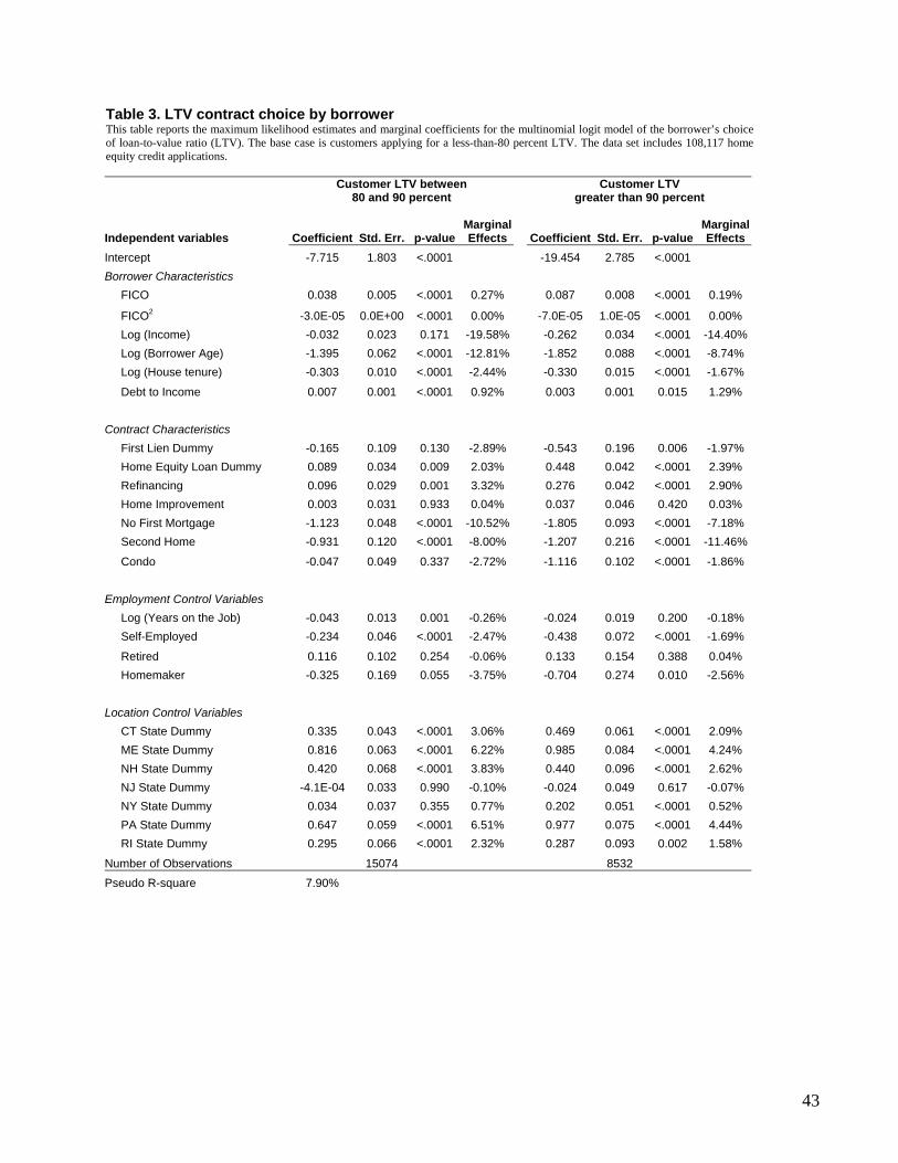
43
Table 3. LTV contract choice by borrower This table reports the maximum likelihood estimates and marginal coefficients for the multinomial logit model of the borrower’s choice of loan-to-value ratio (LTV). The base case is customers applying for a less-than-80 percent LTV. The data set includes 108,117 home equity credit applications.
Customer LTV between 80 and 90 percent
Customer LTV greater than 90 percent
Independent variables
Coefficient Std. Err. p-valueMarginal Effects
Coefficient Std. Err. p-value
Marginal Effects
Intercept -7.715 1.803 <.0001 -19.454 2.785 <.0001 Borrower Characteristics FICO 0.038 0.005 <.0001 0.27% 0.087 0.008 <.0001 0.19%
FICO2 -3.0E-05 0.0E+00 <.0001 0.00% -7.0E-05 1.0E-05 <.0001 0.00% Log (Income) -0.032 0.023 0.171 -19.58% -0.262 0.034 <.0001 -14.40% Log (Borrower Age) -1.395 0.062 <.0001 -12.81% -1.852 0.088 <.0001 -8.74% Log (House tenure) -0.303 0.010 <.0001 -2.44% -0.330 0.015 <.0001 -1.67%
Debt to Income 0.007 0.001 <.0001 0.92% 0.003 0.001 0.015 1.29% Contract Characteristics First Lien Dummy -0.165 0.109 0.130 -2.89% -0.543 0.196 0.006 -1.97% Home Equity Loan Dummy 0.089 0.034 0.009 2.03% 0.448 0.042 <.0001 2.39% Refinancing 0.096 0.029 0.001 3.32% 0.276 0.042 <.0001 2.90% Home Improvement 0.003 0.031 0.933 0.04% 0.037 0.046 0.420 0.03% No First Mortgage -1.123 0.048 <.0001 -10.52% -1.805 0.093 <.0001 -7.18% Second Home -0.931 0.120 <.0001 -8.00% -1.207 0.216 <.0001 -11.46%
Condo -0.047 0.049 0.337 -2.72% -1.116 0.102 <.0001 -1.86% Employment Control Variables Log (Years on the Job) -0.043 0.013 0.001 -0.26% -0.024 0.019 0.200 -0.18% Self-Employed -0.234 0.046 <.0001 -2.47% -0.438 0.072 <.0001 -1.69%
Retired 0.116 0.102 0.254 -0.06% 0.133 0.154 0.388 0.04% Homemaker -0.325 0.169 0.055 -3.75% -0.704 0.274 0.010 -2.56% Location Control Variables CT State Dummy 0.335 0.043 <.0001 3.06% 0.469 0.061 <.0001 2.09% ME State Dummy 0.816 0.063 <.0001 6.22% 0.985 0.084 <.0001 4.24% NH State Dummy 0.420 0.068 <.0001 3.83% 0.440 0.096 <.0001 2.62% NJ State Dummy -4.1E-04 0.033 0.990 -0.10% -0.024 0.049 0.617 -0.07% NY State Dummy 0.034 0.037 0.355 0.77% 0.202 0.051 <.0001 0.52% PA State Dummy 0.647 0.059 <.0001 6.51% 0.977 0.075 <.0001 4.44% RI State Dummy 0.295 0.066 <.0001 2.32% 0.287 0.093 0.002 1.58%
Number of Observations 15074 8532 Pseudo R-square 7.90%
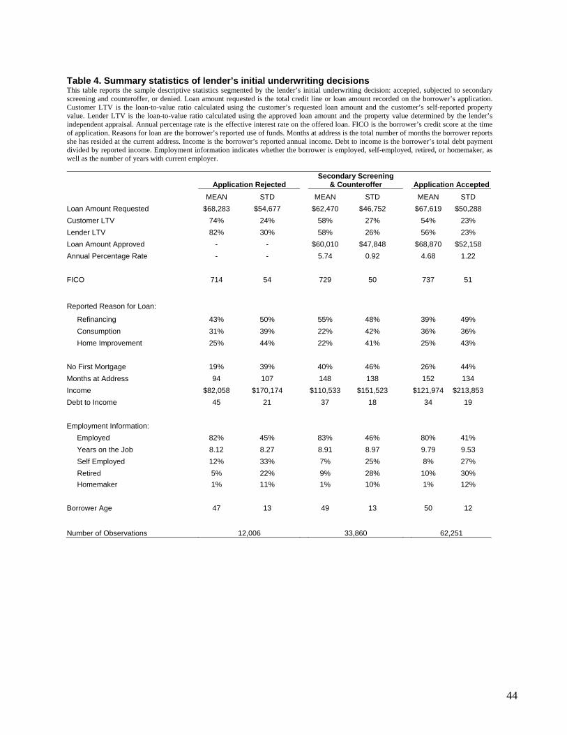
44
Table 4. Summary statistics of lender’s initial underwriting decisions This table reports the sample descriptive statistics segmented by the lender’s initial underwriting decision: accepted, subjected to secondary screening and counteroffer, or denied. Loan amount requested is the total credit line or loan amount recorded on the borrower’s application. Customer LTV is the loan-to-value ratio calculated using the customer’s requested loan amount and the customer’s self-reported property value. Lender LTV is the loan-to-value ratio calculated using the approved loan amount and the property value determined by the lender’s independent appraisal. Annual percentage rate is the effective interest rate on the offered loan. FICO is the borrower’s credit score at the time of application. Reasons for loan are the borrower’s reported use of funds. Months at address is the total number of months the borrower reports she has resided at the current address. Income is the borrower’s reported annual income. Debt to income is the borrower’s total debt payment divided by reported income. Employment information indicates whether the borrower is employed, self-employed, retired, or homemaker, as well as the number of years with current employer.
Application Rejected Secondary Screening
& Counteroffer
Application Accepted MEAN STD MEAN STD MEAN STD
Loan Amount Requested $68,283 $54,677 $62,470 $46,752 $67,619 $50,288 Customer LTV 74% 24% 58% 27% 54% 23% Lender LTV 82% 30% 58% 26% 56% 23% Loan Amount Approved - - $60,010 $47,848 $68,870 $52,158 Annual Percentage Rate - - 5.74 0.92 4.68 1.22 FICO 714 54 729 50 737 51
Reported Reason for Loan:
Refinancing 43% 50% 55% 48% 39% 49% Consumption 31% 39% 22% 42% 36% 36% Home Improvement 25% 44% 22% 41% 25% 43% No First Mortgage 19% 39% 40% 46% 26% 44% Months at Address 94 107 148 138 152 134 Income $82,058 $170,174 $110,533 $151,523 $121,974 $213,853 Debt to Income 45 21 37 18 34 19 Employment Information: Employed 82% 45% 83% 46% 80% 41% Years on the Job 8.12 8.27 8.91 8.97 9.79 9.53 Self Employed 12% 33% 7% 25% 8% 27% Retired 5% 22% 9% 28% 10% 30% Homemaker 1% 11% 1% 10% 1% 12% Borrower Age 47 13 49 13 50 12
Number of Observations 12,006 33,860 62,251

45
Table 5. Counteroffer and credit rationing by lender This table reports the estimated coefficients and marginal effects for the maximum likelihood estimation of the multinomial logit model of the lender’s initial underwriting decision. The base case is loans that were accepted outright (without additional screening). Lender LTV 80-90 is a dummy variable indicating loans with actual LTV ratios between 80 and 90 percent. Lender LTV 90+ is a dummy variable indicating loans with actual LTV ratios greater than 90 percent. The data set includes 108,117 home equity credit applications.
Subjected to Secondary Screening and
Counteroffer
Application Rejected
Independent variables Coeff.
Val. Std. Err. p-valueMarginal Effects
Coeff. Val. Std. Err. p-value
Marginal Effects
Intercept -10.914 1.210 <.0001 -0.020 1.665 0.990 Borrower Characteristics
FICO 0.032 0.003 <.0001 0.08% 0.008 0.002 <.0001 0.09%
FICO2 -2.0E-05 4.0E-06 <.0001 0.00% -3.0E-04 6.0E-05 0.002 0.00% Log (Income) -0.115 0.015 <.0001 -2.55% -0.018 0.002 <.0001 -3.79% Log (House tenure) -0.015 0.007 0.038 -0.32% -0.067 0.011 <.0001 -0.23% Debt to Income 0.002 0.001 <.0001 0.95% 0.005 0.001 <.0001 1.78% Contract Characteristics Lender LTV 80-90 1.282 0.021 <.0001 12.01% 1.652 0.033 <.0001 8.67% Lender LTV 90+ 2.223 0.036 <.0001 15.84% 3.921 0.041 <.0001 18.35% First Lien Dummy 4.846 0.134 <.0001 17.13% -3.429 0.146 <.0001 -12.18% Home Equity Loan Dummy 0.379 0.022 <.0001 6.71% 0.959 0.031 <.0001 4.77% Home Improvement -0.041 0.021 0.504 -0.17% -0.028 0.033 0.390 -0.12% Refinancing -0.048 0.011 <.0001 -3.68% -0.174 0.030 <.0001 -2.61% No First Mortgage 0.021 0.002 <.0001 1.66% -0.367 0.038 <.0001 -1.18% Second Home 0.346 0.052 <.0001 8.64% 1.377 0.061 <.0001 6.14% Condo 0.490 0.032 <.0001 9.07% 1.305 0.041 <.0001 6.45% Employment Control Variables Log (Years on the Job) -0.031 0.009 0.000 -0.43% -0.060 0.013 <.0001 -0.31% Self Employed 0.055 0.030 0.064 3.04% 0.733 0.039 <.0001 2.16% Retired -0.246 0.120 0.040 -1.54% -0.115 0.187 0.541 -1.10% Homemaker -0.153 0.044 0.001 -1.75% -0.216 0.078 0.005 -1.24%
Location Control Variables
CT State Dummy -0.072 0.030 0.018 -2.09% -0.357 0.048 <.0001 -1.49% ME State Dummy -0.116 0.048 0.016 -3.90% -0.737 0.083 <.0001 -2.77% NH State Dummy -0.075 0.051 0.138 -1.81% -0.323 0.079 <.0001 -1.29% NJ State Dummy 0.004 0.022 0.847 -0.52% -0.089 0.033 0.007 -0.37% NY State Dummy -0.078 0.024 0.002 -1.26% -0.153 0.037 <.0001 -0.90% PA State Dummy -0.005 0.043 0.907 -0.80% -0.115 0.060 0.057 -0.57% RI State Dummy -0.110 0.048 0.021 -1.98% -0.306 0.075 <.0001 -1.41%
Number of Observations 33,860 12,006 Pseudo R-square 11.34%

46
Table 6. Test of adverse selection on unobservable risk characteristics This table reports the competing risks hazard model of loan default and prepayment in order to identify the presence of adverse selection in the set of 62,251 applicants who were accepted outright (without secondary screening). The base case is that the loan remains current as of the end of the observation period (March 2005). CLTV is the current (time-varying) loan-to-value ratio based on estimated changes in the underlying house price obtained from the OFHEO MSA level repeat sales indices. PPOption captures the borrower’s prepayment option value. LTV difference is a dummy variable denoting a decline in collateral value from the previous quarter. House value difference is the percentage difference between the borrower’s initial house value and the lender’s independent appraisal. Account age is the number of months since origination and controls for loan seasoning. The model is estimated by maximum likelihood treating both prepayment and default outcomes as correlated competing risk estimated jointly. A bivariate distribution of unobserved heterogeneous error terms is also estimated simultaneously with the competing risk hazard. LOC1 and LOC2 are the location parameters and MASS2 is the mass points associated with LOC1 (MASS1 is normalized to 1).
Default Prepayment
Independent variables Coeff. Val.
Std. Err. p-value
Marginal Effects
Coeff. Val. Std. Err. p-value
Marginal Effects
Intercept 24.075 1.173 <.0001 -2.520 0.357 <.0001 Borrower Characteristics
FICO -0.182 0.012 <.0001 -0.49% 0.052 0.003 <.0001 0.15%
FICO2 1.1E-04 9.1E-06 <.0001 0.00% 4.0E-05 1.8E-06 <.0001 0.00% Log (Income) -0.377 0.082 <.0001 -9.49% 0.180 0.016 <.0001 1.95% Log (House tenure) -0.213 0.031 <.0001 -9.44% -0.101 0.007 <.0001 -1.74% Debt to Income 0.026 0.003 <.0001 2.06% 0.017 0.001 <.0001 2.24%
Contract Characteristics
Lender LTV 80-90 0.354 0.125 0.005 2.22% -0.553 0.021 <.0001 -4.53% Lender LTV 90+ 1.291 0.180 <.0001 5.57% -1.709 0.052 <.0001 -6.57% Home Equity Loan Dummy 1.929 0.192 <.0001 5.38% 0.995 0.051 <.0001 2.07% First Lien Dummy -0.653 0.090 <.0001 -2.26% -0.732 0.107 <.0001 -2.14% Refinancing -0.521 0.110 <.0001 -3.70% 0.165 0.018 <.0001 2.77% Home Improvement -0.681 0.115 <.0001 -3.36% 0.043 0.021 0.042 1.41%
No First Mortgage -1.133 0.137 <.0001 -6.79% -0.120 0.022 <.0001 -3.10% Second Home 3.140 0.150 <.0001 2.08% -0.259 0.043 <.0001 -3.10% Condo -2.251 0.345 <.0001 -1.26% 0.568 0.034 <.0001 2.46% Auto Pay -0.360 0.099 0.000 -4.18% 0.060 0.017 0.001 2.72%
Time-varying Option Variables
CLTV 0.188 0.368 <.0001 3.98% -0.489 0.038 <.0001 -1.03%
CLTV2 1.288 0.384 <.0001 8.91% -0.691 0.061 <.0001 -4.30% PPOption 1.433 0.262 <.0001 3.05% 1.128 0.215 <.0001 8.12% LTV_Diff_Dummy 1.012 0.218 <.0001 2.98% -0.624 0.034 <.0001 -1.14%
HouseVal_Diff 0.345 0.074 <.0001 2.26% -0.204 0.038 <.0001 -2.10% Account Age 0.047 0.019 0.013 1.07% -0.189 0.037 <.0001 -2.71%
Account Age2 -4.4E-04 9.1E-05 <.0001 -2.55% 1.9E-03 1.9E-05 <.0001 1.02%
Account Age3 2.0E-06 2.0E-07 <.0001 0.58% 3.0E-06 2.0E-06 <.0001 0.35% Employment Control Variables
Log (Years on the Job) -0.341 0.047 <.0001 -4.03% -0.072 0.008 <.0001 -1.00% Self Employed 0.630 0.094 <.0001 0.19% -0.499 0.026 <.0001 -1.58% Retired 1.279 0.196 <.0001 0.32% 0.852 0.041 <.0001 2.77% Homemaker -0.928 1.153 0.421 -0.65% -1.111 0.165 <.0001 -2.53%
Location and Economic Control Variables
Unemployment Rate 0.358 0.023 <.0001 1.62% 0.046 0.005 <.0001 3.80%

47
CT State Dummy -1.465 0.249 <.0001 -0.07% 0.201 0.022 <.0001 2.87% ME State Dummy -1.974 1.114 0.076 -0.30% 0.677 0.058 <.0001 0.85% NH State Dummy 0.348 0.109 <.0001 0.47% 0.378 0.059 <.0001 0.79% NJ State Dummy -1.203 0.202 <.0001 -0.02% 0.055 0.028 0.052 0.90% NY State Dummy 0.235 0.105 0.025 0.03% 0.082 0.021 0.000 1.31% PA State Dummy 1.035 0.116 <.0001 0.13% 0.282 0.039 <.0001 0.97% RI State Dummy -1.593 0.473 0.001 -0.16% 0.438 0.043 <.0001 0.31% Unobserved Heterogeneity Factors
Loc1 1.479 0.489 <.0001 0.974 0.130 <.0001 Loc2 1.698 0.572 <.0001 0.899 0.286 <.0001 Mass2 0.489 0.128 <.0001 0.685 0.184 <.0001 Time Quarter Dummies Yes
Pseudo R-square 13.06% Number of Accts/Defaults/Prepay 702
20399

48
Table 7. Summary statistics of counteroffers by mitigation type This table reports the descriptive statistics for the variables used in the analysis of the lender’s decision about whether the 33,860 borrower applications who are subjected to secondary screening should receive either a counteroffer designed to mitigate adverse selection or one designed to counteroffer moral hazard. Loan amount requested is the total credit line or loan amount recorded on the borrower’s application. Loan amount approved is the actual credit amount offered. Customer LTV is the loan-to-value ratio calculated using the customer’s requested loan amount and the customer’s self-reported property valuation. Lender LTV is the loan-to-value ratio calculated using the approved loan amount and the property value determined by the lender’s independent appraisal. Annual percentage rate is the effective interest rate on the offered loan. FICO is the borrower’s credit score at the time of application. Reasons for loan are the borrower’s reported use of funds. Months at address is the total number of months the borrower reports she has resided at the current address. Income is the borrower’s reported annual income. Debt to income is the borrower’s total debt payment divided by reported income. Employment information indicates whether the borrower is employed, self-employed, retired, or homemaker, as well as the number of years with current employer.
Moral Hazard Mitigation Adverse Selection Mitigation MEAN STD MEAN STD Loan Amount Requested $68,441 $50,808 $47,703 $36,825
Loan Amount Approved $64,868 $52,049 $47,903 $37,284 Customer LTV 56% 28% 63% 23% Lender LTV 54% 28% 67% 23% APR 4.89 0.93 7.60 0.88 FICO 727 48 719 53 Reported Reason for Loan: Refinancing 64% 48% 38% 48% Home Improvement 21% 40% 25% 44% Consumption 16% 43% 37% 40% No First Mortgage 48% 48% 22% 41% Months at Address 158 144 127 126 Income $118,659 $113,800 $92,797 $94,722 Debt to Income 35 18 40 19 Employment Information Employed 84% 46% 82% 45% Yeas on the Job 8.99 8.94 8.73 9.02 Self Employed 8% 27% 5% 21% Retired 8% 26% 12% 32% Homemaker 1% 11% 1% 10% Borrower Age 49 13 47 13
Frequency 23,222 10,638
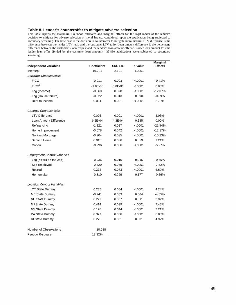
49
Table 8. Lender’s counteroffer to mitigate adverse selection This table reports the maximum likelihood estimates and marginal effects for the logit model of the lender’s decision to mitigate for adverse selection or moral hazard, conditional upon the application being subjected to secondary screening. The base case is the decision to counteroffer to mitigate moral hazard. LTV difference is the difference between the lender LTV ratio and the customer LTV ratio. Loan amount difference is the percentage difference between the customer’s loan request and the lender’s loan amount offer (customer loan amount less the lender loan offer divided by the customer loan amount). 33,860 applications were subjected to secondary screening.
Independent variables Coefficient Std. Err. p-value Marginal Effects
Intercept 10.781 2.101 <.0001 Borrower Characteristics FICO -0.011 0.003 <.0001 -0.41%
FICO2 -1.0E-05 3.0E-06 <.0001 0.00% Log (Income) -0.669 0.028 <.0001 -12.07% Log (House tenure) -0.022 0.013 0.090 -0.39% Debt to Income 0.004 0.001 <.0001 2.79% Contract Characteristics LTV Difference 0.005 0.001 <.0001 3.08% Loan Amount Difference 6.5E-04 4.3E-04 0.385 0.00% Refinancing -1.221 0.037 <.0001 -21.94% Home Improvement -0.678 0.042 <.0001 -12.17% No First Mortgage -0.904 0.035 <.0001 -16.23% Second Home 0.015 0.086 0.859 7.21% Condo -0.296 0.056 <.0001 -5.27% Employment Control Variables Log (Years on the Job) -0.036 0.015 0.016 -0.65% Self Employed -0.420 0.059 <.0001 -7.52% Retired 0.372 0.073 <.0001 6.69% Homemaker -0.310 0.229 0.177 -0.56% Location Control Variables CT State Dummy 0.235 0.054 <.0001 4.24% ME State Dummy -0.241 0.083 0.004 -4.35% NH State Dummy 0.222 0.087 0.011 3.97%
NJ State Dummy 0.414 0.039 <.0001 7.45% NY State Dummy 0.178 0.044 <.0001 3.21% PA State Dummy 0.377 0.066 <.0001 6.80% RI State Dummy 0.275 0.081 0.001 4.92%
Number of Observations 10,638 Pseudo R-square 13.32%
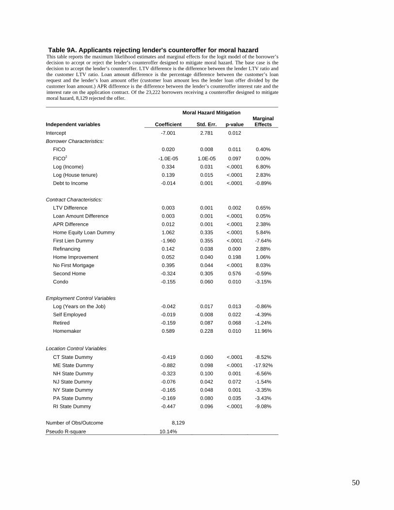
50
Table 9A. Applicants rejecting lender's counteroffer for moral hazard This table reports the maximum likelihood estimates and marginal effects for the logit model of the borrower’s decision to accept or reject the lender’s counteroffer designed to mitigate moral hazard. The base case is the decision to accept the lender’s counteroffer. LTV difference is the difference between the lender LTV ratio and the customer LTV ratio. Loan amount difference is the percentage difference between the customer’s loan request and the lender’s loan amount offer (customer loan amount less the lender loan offer divided by the customer loan amount.) APR difference is the difference between the lender’s counteroffer interest rate and the interest rate on the application contract. Of the 23,222 borrowers receiving a counteroffer designed to mitigate moral hazard, 8,129 rejected the offer.
Moral Hazard Mitigation
Independent variables Coefficient Std. Err. p-value Marginal Effects
Intercept -7.001 2.781 0.012 Borrower Characteristics: FICO 0.020 0.008 0.011 0.40%
FICO2 -1.0E-05 1.0E-05 0.097 0.00% Log (Income) 0.334 0.031 <.0001 6.80% Log (House tenure) 0.139 0.015 <.0001 2.83% Debt to Income -0.014 0.001 <.0001 -0.89% Contract Characteristics: LTV Difference 0.003 0.001 0.002 0.65% Loan Amount Difference 0.003 0.001 <.0001 0.05% APR Difference 0.012 0.001 <.0001 2.38% Home Equity Loan Dummy 1.062 0.335 <.0001 5.84% First Lien Dummy -1.960 0.355 <.0001 -7.64% Refinancing 0.142 0.038 0.000 2.88% Home Improvement 0.052 0.040 0.198 1.06% No First Mortgage 0.395 0.044 <.0001 8.03% Second Home -0.324 0.305 0.576 -0.59% Condo -0.155 0.060 0.010 -3.15% Employment Control Variables Log (Years on the Job) -0.042 0.017 0.013 -0.86% Self Employed -0.019 0.008 0.022 -4.39% Retired -0.159 0.087 0.068 -1.24% Homemaker 0.589 0.228 0.010 11.96%
Location Control Variables
CT State Dummy -0.419 0.060 <.0001 -8.52% ME State Dummy -0.882 0.098 <.0001 -17.92% NH State Dummy -0.323 0.100 0.001 -6.56% NJ State Dummy -0.076 0.042 0.072 -1.54% NY State Dummy -0.165 0.048 0.001 -3.35% PA State Dummy -0.169 0.080 0.035 -3.43% RI State Dummy -0.447 0.096 <.0001 -9.08% Number of Obs/Outcome 8,129
Pseudo R-square 10.14%

51
Table 9B. Applicants rejecting lender's counteroffer for adverse selection This table reports the maximum likelihood estimates and marginal effects for the logit model of the borrower’s decision to accept or reject the lender’s counteroffer designed to mitigate adverse selection. The base case is the decision to accept the lender’s counteroffer. LTV difference is the difference between the lender LTV ratio and the customer LTV ratio. Loan amount difference is the percentage difference between the customer’s loan request and the lender’s loan amount offer (customer loan amount less the lender loan offer divided by the customer loan amount.) APR difference is the difference between the lender’s counteroffer interest rate and the interest rate on the application contract. Of the 10,638 borrowers receiving a counteroffer designed to mitigate adverse selection, 4,571 rejected the offer.
Adverse Selection Mitigation
Independent variables Coefficient Std. Err. p-value Marginal Effects
Intercept -5.986 3.947 0.129 Borrower Characteristics FICO -0.010 0.010 0.329 -0.18%
FICO2 1.0E-05 1.0E-05 0.109 0.00% Log (Income) 0.534 0.052 <.0001 9.77% Log (House tenure) 0.001 0.025 0.982 3.01% Debt to Income -0.006 0.002 0.001 -0.91% Contract Characteristics LTV Difference 0.002 0.001 0.128 0.32% Loan Amount Difference 0.004 0.001 0.001 0.07% APR Difference 0.165 0.006 <.0001 1.02% Home Equity Loan Dummy -4.389 1.371 0.001 -8.28% First Lien Dummy -2.996 0.166 <.0001 -5.81% Refinancing -0.219 0.074 0.003 -4.01% Home Improvement -0.129 0.086 0.133 -2.35% No First Mortgage 1.382 0.166 <.0001 24.29% Second Home -0.245 0.054 <.0001 -4.48% Condo -0.203 0.102 0.046 3.71% Employment Control Variables Log (Years on the Job) -0.070 0.027 0.010 -1.27% Self Employed 0.055 0.112 0.623 1.01% Retired -0.486 0.131 0.000 -8.88% Homemaker -0.714 0.431 0.098 -13.06%
Location Control Variables
CT State Dummy -0.761 0.102 <.0001 -13.92% ME State Dummy -0.736 0.162 <.0001 -13.47% NH State Dummy -0.247 0.154 0.109 -4.52% NJ State Dummy -0.231 0.073 0.002 -4.23% NY State Dummy -0.757 0.081 <.0001 -13.84% PA State Dummy -0.346 0.114 0.003 -6.32% RI State Dummy -0.317 0.141 0.024 -5.80%
Number of Obs/Outcome 4,571 Pseudo R-square 12.56%

52
Table 10. Effectiveness of lender’s effort to mitigate adverse selection and moral hazard This table reports the competing risks hazard model of loan default and prepayment in order to identify the effect of the lender’s efforts at mitigating adverse selection and moral hazard in the set of 83,411 applications that are ultimately booked. The base case is that the loan remains current as of the end of the observation period (March 2005). CLTV is the current (time-varying) loan-to-value ratio based on estimated changes in the underlying house price obtained from the OFHEO MSA level repeat sales indices. PPOption captures the borrower’s prepayment option value. LTV difference is a dummy variable denoting a decline in collateral value from the previous quarter. House value difference is the percentage difference between the borrower’s initial house value and the lender’s independent appraisal. Account age is the number of months since origination and controls for loan seasoning. The model is estimated by maximum likelihood treating both prepayment and default outcomes as correlated competing risk estimated jointly. A bivariate distribution of unobserved heterogeneous error terms is also estimated simultaneously with the competing risk hazard. LOC1 and LOC2 are the location parameters and MASS2 is the mass points associated with LOC1 (MASS1 is normalized to 1).
Default Prepayment
Independent variables Coeff. Val.
Std. Err. p-value
Marginal Effects
Coeff. Val.
Std. Err.
p-value
Marginal Effects
Intercept 40.018 3.500 <.0001 -17.475 0.728 <.0001 Borrower Characteristics
FICO -0.101 0.010 <.0001 -0.50% 0.043 0.002 <.0001 0.20% FICO2 5.0E-05 1.0E-05 <.0001 0.01% 3.0E-05 0.0E+00 <.0001 0.01% Log (Income) -0.142 0.060 0.017 -9.10% 0.248 0.013 <.0001 3.40% Log (House tenure) -0.051 0.023 0.028 -10.00% -0.020 0.006 0.000 -1.40% Debt to Income 0.019 0.002 <.0001 2.00% 0.015 4.1E-04 <.0001 2.20%
Contract Characteristics
Moral Hazard Mitigation -0.184 0.067 0.006 -12.2% 0.649 0.016 <.0001 11.0% Adverse Selection Mitigation 0.649 0.131 <.0001 4.20% 0.232 0.027 <.0001 2.90% Home Equity Loan Dummy 3.809 0.152 <.0001 6.40% 1.205 0.039 <.0001 1.90% First Lien Dummy -0.272 0.159 0.087 -1.20% -0.760 0.036 <.0001 -3.10%
Refinancing -0.372 0.073 <.0001 -3.10% 0.155 0.014 <.0001 3.00% Home Improvement -0.408 0.082 <.0001 -4.00% 0.086 0.017 <.0001 2.00%
No First Mortgage -0.155 0.100 0.121 -5.10% -0.181 0.019 <.0001 -3.90% Second Home 1.775 0.107 <.0001 2.00% -0.133 0.033 <.0001 -2.20% Condo -2.773 0.247 <.0001 -1.2% 0.664 0.026 <.0001 2.90%
BorrLender_Diff -1.237 0.265 <.0001 -6.90% 0.824 0.174 <.0001 7.30% Time-varying Option Variables
CLTV 0.118 0.089 0.185 2.10% -0.307 0.017 <.0001 -5.40% CLTV2 1.089 0.128 <.0001 1.30% -0.802 0.032 <.0001 -3.80% Auto Pay -0.255 0.070 0.000 -4.00% 0.052 0.013 0.000 5.70% PPOption 3.007 0.445 <.0001 5.00% 2.096 0.711 <.0001 9.00% LTV_Diff_Dummy 1.027 0.189 <.0001 2.00% -0.313 0.090 <.0001 -1.10%
HouseVal_Diff 0.689 0.144 <.0001 2.60% -0.195 0.028 <.0001 -2.50% Account Age 6.0E-03 1.6E-03 0.000 1.40% -6.3E-03 2.9E-04 <.0001 -3.70% Account Age2 -3.2E-03 5.8E-04 <.0001 -2.20% 2.0E-04 2.5E-04 0.413 2.40% Account Age3 1.0E-05 0.0E+00 <.0001 0.50% 0.0E+00 0.0E+00 <.0001 0.40%
Employment Control Variables
Log (Years on the Job) -0.389 0.035 <.0001 -4.00% -0.008 0.006 0.186 -0.30% Self Employed 0.295 0.076 <.0001 0.30% -0.238 0.019 <.0001 -3.70% Retired 0.913 0.150 <.0001 0.20% 0.544 0.033 <.0001 2.10% Homemaker -0.991 1.013 0.328 -0.60% -1.439 0.145 <.0001 -3.40%
Location and Economic Control Variables

53
Unemployment Rate 0.193 0.018 <.0001 1.30% 1.4E-04 4.2E-03 0.973 3.00% CT State Dummy -1.791 0.160 <.0001 0.01% 0.157 0.017 <.0001 1.20% ME State Dummy -2.814 1.006 0.005 -0.10% 0.254 0.045 <.0001 1.10% NH State Dummy 0.343 0.073 <.0001 0.10% 0.473 0.076 <.0001 1.00% NJ State Dummy -0.749 0.127 <.0001 0.01% -0.093 0.023 <.0001 -1.00% NY State Dummy -0.340 0.078 <.0001 0.01% 0.128 0.017 <.0001 2.20% PA State Dummy 0.470 0.094 <.0001 0.01% -0.025 0.030 0.409 -0.30% RI State Dummy -1.325 0.330 <.0001 -0.10% 0.252 0.037 <.0001 0.60%
Unobserved Heterogeneity Factors
Loc1 2.739 0.376 <.0001 1.896 0.349 <.0001 Loc2 1.358 0.373 <.0001 1.578 0.387 <.0001 Mass2 0.980 0.088 <.0001 0.635 0.074 <.0001
Time Quarter Dummies Yes Yes Pseudo R-square 12.32%
Number of Obs/Defaults 916 32860

54
Appendix A: Competing Risk Model with Unobserved Heterogeneity
In estimating the competing risks hazard model, we follow the procedure outlined
in Agarwal et al. (2006) and denote credit commitments that are still current at the end of
the observation period as censored. We assume that the time to prepayment, Tp, and time to
default, Td, are random variables that have continuous probability distributions, f(tj), where
tj is a realization of Tj (j=p,d). The joint survivor function conditional on factors θp, θd, r,
H, X, and Z, S(tp,td|r,H,X,Z,θp,θd)=Pr(Tp>tp,Td>td|r,H,X,Z,θp,θd), is defined as
( ) ( )( )
( )( )),,exp
,,expexp(,,,,,|,
1
'
1
'
∑
∑
=
=
++−
++−=
d
p
t
nddndnd
t
nppnpnpdpdp
ZXHrg
ZXHrgZXHrttS
βαθ
βαθθθ , (3.)
where gjn(r,H,X) is a time-varying function of the relevant interest rates (r), property values
(H), and borrower characteristics (X), Z represents macro-economic factors (possibly time-
varying), and θp and θd are the unobservable heterogeneity factors.25 The parameters αjn
are the baseline hazard parameters estimated as
( ) ⎥⎦⎤
⎢⎣⎡= ∫ −
n
n jjn dtt1
log λα , (4.)
where λj(t) is the underlying continuous-time baseline hazard function, and j=p,d.
Following Deng, Quigley, and Van Order (2000), we note that the data set consists
of M distinct borrower groups, with the distribution of unobservable heterogeneity factors
(θp and θd) modeled by assuming that the unobserved borrower types occur with frequency
γm, m=1…M. Furthermore, following McCall (1996), we note that only the duration
25 See McCall (1996) appendix B.

55
associated with a particular termination type is observed (t=min(tp,td)). Thus, we define the
following probabilities:26
( ) ( ) ( ) ( )( ) ( ) ( )},|,1,|1,,|1,1
,|,{5.,|,1,|,,|
dpdpdp
dpdpdpdpp
ttSttSttS
ttSttSttStA
θθθθθθ
θθθθθθθθ
+−+−+++
−+−= , (5.)
( ) ( ) ( ) ( )( ) ( ) ( )},|,1,|1,,|1,1
,|,{5.,|,1,|,,|
dpdpdp
dpdpdpdpd
ttSttSttS
ttSttSttStA
θθθθθθ
θθθθθθθθ
+−+−+++
−+−= , (6.)
and
( ) ( )dpdpc ttStA θθθθ ,|,,| = . (7.)
The probabilities of mortgage termination by prepayment and default are represented by
the functions Ap and Ad, respectively, while Ac represents the probability that the
observation is censored due to the ending of the data collection period. The term in braces
in equations (3) and (4) is the adjustment factor necessary due to discrete time
measurement of duration.
The unconditional probabilities are given by
( ) ( ) cdpjtAtAM
mdmpmjmj ,,,,|
1== ∑
=
θθγ , (8.)
and the log-likelihood function of the competing risks model is given by
( )( ) ( )( ) ( )( )∑=
++=N
iicciiddiippi TATATAL
1loglogloglog δδδ , (9.)
where δij, j=p,d,c are indicator variables denoting that the ith loan is terminated by
prepayment or default, or is censored. Equation (9) is estimated via maximum likelihood.
26 The dependence of the functions in equations (3)-(5) on r, H, X, and Z has been omitted for ease of exposition.

56
Appendix B: Control Variables Used in Estimation of Competing Risks Models
In modeling the loan performance, we follow the previous empirical studies of
mortgage performance and incorporate a set of explanatory variables that capture borrower
financial incentives to prepay or default. For example, to approximate the value of the
borrower’s prepayment option, we follow the approach outlined in Deng, Quigley, and
Van Order (2000) and estimate the prepayment option as
ti
tititi V
VVPPOption
,
*,,
,−
= , (10.)
where Vi,t is the market value of loan i at time t (i.e., the present value of the remaining
mortgage payments at the current market mortgage rate), and *,tiV is the book-value of loan
i at time t (i.e., the present value of the remaining mortgage payments at the contract
interest rate).27 We calculate Vi,t by using the current period t market interest rate on home
equity lines and home equity loans, respectively.28 Since consumers are more likely to
prepay and refinance following a decline in the prevailing mortgage rate relative to the
original coupon rate, a positive value for PPOption is indicative of an “in-the-money”
prepayment option. In order to account for any non-linearity in the prepayment option, we
also include the square of PPOption.
To determine the impact of changing property values on loan and line termination
probabilities, we matched each observation with the quarterly OFHEO MSA level repeat
sales indices. Based on the estimated changes in house prices, we construct time-varying
loan-to-value ratios (CLTV) where the loan value is the total outstanding loan balance that
27 This is equivalent to the prepayment option value used by Archer, Ling, and McGill (1996) scaled by the mortgage book-value. 28 Current period t home equity line and home equity loan market interest rates were obtained from the Heitman Group (www.heitman.com).

57
includes the first mortgage.29 We also include the square of CLTV to control for any non-
linearity. We include a dummy variable for a positive quarterly change in the loan-to-value
ratio (LTV_Diff_Dummy) to capture the changes in default option values.30
Related to the role of collateral in impacting termination probabilities, we also
include the percentage difference between the borrower’s initial house value assessment
and the lender’s independent appraised value (HouseVal_Diff). Agarwal (2006) finds that
borrowers who underestimate their house value are more likely to refinance without cash
and prepay their loans while borrowers who overestimate their house value are more likely
to cash out and default on their loans. Thus, the percentage difference in valuation
estimates (HouseVal_Diff ) provides a rough proxy for the borrower’s risk aversion.
We capture changes in borrower credit constraints via the time-varying borrower
credit score (FICO) and include the square of FICO to capture any non-linearity present in
borrower credit scores. Borrowers with good credit history (higher FICO scores) are able
to obtain credit with ease; thus, they are able to take advantage of refinancing
opportunities. Conversely, borrowers with lower credit scores may be credit-constrained
(see Peristiani et al., 1997; and Bennet, Peach, and Peristiani, 2000). Similarly, Agarwal,
Ambrose, and Liu (2006) show that liquidity-constrained borrowers (e.g., borrowers with
deteriorating credit quality) who have home equity lines are more likely to raise their
utilization rates rather than pay down the line.
Local economic conditions may also impact mortgage termination decisions. For
example, Hurst and Stafford (2004) note that borrowers with uncertain job prospects may
29 See Agarwal, Ambrose, and Liu (2006) for a discussion of the potential bias present in the CLTV ratio. 30 LTV_Diff_Dummy is set equal to one if CLTVt – CLTVt-1 is greater than zero. Thus, a positive value for LTV_Diff_Dummy indicates that the collateral value has declined from the previous quarter resulting in an increase in the current loan-to-value ratio.

58
refinance in order to tap into their accumulated equity. Thus, we use the current county
unemployment rate (UnempRate) as a proxy for local economic conditions. We also
include a series of dummy variables that denote the borrower’s location (state) to control
for unobserved state-specific factors.
We also include a number of variables to control for account seasoning (AGE of
account, and AGE-square), and calendar time effects. AGEi,t is the number of months since
origination at time t, and, as Gross and Souleles (2002) point out, allows for loan
seasoning. That is, AGE accounts for changes in the default propensity as loans mature. In
addition, Gross and Souleles (2002) note that the age variables allow the hazard rates to
vary with duration. Our quadratic specification of AGE allows the default hazard to vary
non-parametrically. The dummy variables corresponding to calendar quarters (Q3:99—
Q1:02) at origination capture unobserved shifts over time in economic conditions or
borrower characteristics that may impact the propensity default.
Finally, we include as control variables the information collected from the loan
application that indicate the borrower’s employment status (e.g., employed, self-employed,
retired, or homemaker), number of years employed, the borrower’s income at the time of
application, the property type (single-family detached or condo), the property’s status as
primary residence or second home, the tenure in the property, the use of the funds (e.g.,
refinancing, home-improvement, or debt consolidation), the current existence of a first
mortgage on the property, and the borrower’s use of an “auto-draft” feature to
automatically make the monthly payment.
Recommended

![Signaling equilibria for dynamic LQG games with asymmetric ...arXiv:1606.04960v1 [cs.GT] 15 Jun 2016 Signaling equilibria for dynamic LQG games with asymmetric information Deepanshu](https://img.pdfslide.net/doc/110x75/5e8c0d64105ba34e03071329/signaling-equilibria-for-dynamic-lqg-games-with-asymmetric-arxiv160604960v1.jpg)

![1 Dynamic Games with Asymmetric Information: Common ... › pdf › 1510.07001.pdf · resemble Markov perfect equilibrium (MPE), defined in [18] for dynamic games with symmetric](https://img.pdfslide.net/doc/110x75/5f0493727e708231d40ea722/1-dynamic-games-with-asymmetric-information-common-a-pdf-a-151007001pdf.jpg)