1
Atmospheric contribution to Mediterranean and nearby 1
Atlantic sea level variability under different climate 2
change scenarios 3
4
G. Jordà, D. Gomis, E. Álvarez-Fanjul, S. Somot 5
Published in Global and Planetary Change 80-81 (2012) 198–214 6
doi:10.1016/j.gloplacha.2011.10.013 7
8
Abstract 9
The contribution of atmospheric pressure and wind to the XXI century sea level 10
variability in Southern Europe is explored under different climate change scenarios. The 11
barotropic version of the HAMSOM model is forced with the output of the atmospheric 12
ARPEGE model run under scenarios B1, A1B and A2. Additionally, a control 13
simulation forced by observed SST, GHGs and aerosols concentrations for the period 14
1950-2000 and a hindcast forced by a dynamical downscalling of ERA40 for the period 15
1958-2001 are also run using the same models. The hindcast results have been validated 16
against tide gauge observations showing good agreement with correlations around 0.8 17
and root mean square error of 3.2 cm. A careful comparison between the control 18
simulation and the hindcast shows a reasonably good agreement between both runs in 19
statistical terms, which points towards the reliability of the modelling system when it is 20
forced only by GHG and aerosols concentrations. The results for the XXI century 21
indicate a sea level decrease that would be especially strong in winter, with trends of up 22
to -0.8 + 0.1 mm/year in the central Mediterranean under the A2 scenario. Trends in 23
summer are small but positive (~0.05 + 0.04 mm/yr), then leading to an increase in the 24
amplitude of the seasonal cycle. The interannual variability also shows some changes, 25
the most important being a widespread standard deviation increase of up to 40%. An 26
increase in the frequency of positive phases of the NAO explains part of the winter 27
negative trends. Also, an increase in the NAO variability would be responsible for the 28
projected increase of the interannual variability of the atmospheric component of sea 29
level. Conversely, the intra-annual variability (1-12 months excluding the seasonal 30
cycle) does not show significant changes. 31
32
2
1. Introduction 33
Sea level variability spans a wide frequency range: storm surges and tides, the seasonal 34
cycle, inter-annual to secular variability and, finally, variations at geological and 35
interglacial scales. Some of these frequencies are better understood and can be easily 36
predicted, as the tidal components. Other processes like those related to inter-annual to 37
centennial changes are less known. 38
Because coastal development is designed on the basis of present mean sea level and its 39
short-term variability (i.e., meteorological fluctuations and tides), a better knowledge of 40
slower processes is necessary for assessing the long-term security of coastal settlements. 41
Physical processes associated with slow mean sea level variations are beach erosion, 42
flooding related to storm surges, damage on harbour structures caused by wind waves or 43
intrusion of salt in fresh water streams and reservoirs (see e.g. Nicholls and Leatherman, 44
1994). All these effects are particularly important for Southern Europe, where a large 45
part of the economy relies directly or indirectly on shore activities. 46
Present knowledge on long term sea level trends in Southern Europe comes mostly from 47
tide gauge records. Marcos and Tsimplis (2008a) studied the five tide gauges that span 48
most of the 20th century and obtained positive trends between 1.2 and 1.5±0.1 mm/yr, 49
that is, of the same order than the average global mean sea level rise observed during 50
the same period (1–2 mm/yr, see for instance Douglas, 2001; IPCC, 2007). For the 51
second half of the 20th century, however, the 21 longest records (>35 yr) in the region 52
show trends between −0.3±0.3 and −1.5±0.4 mm/yr in the Mediterranean Sea and 53
between 1.6±0.5 and –1.9±0.5 mm/yr in the neighbouring Atlantic sites (all computed 54
for the period 1960–2000, see Marcos and Tsimplis, 2008a). In order to avoid the 55
spatial bias of tide gauges, which are mostly located in the northern Mediterranean 56
shores, Calafat and Gomis (2009) reconstructed sea levels fields for the period 1945-57
2000 from a reduced space optimal interpolation of altimetry and tide gauge data. The 58
Mediterranean mean sea level trends computed from the reconstruction are 0.6±0.1 59
mm/yr for the period 1945-2000 and 0.2±0.1 mm/yr for the period 1961-2000; that is, 60
larger than the tide gauge trends given by Marcos and Tsimplis (2008a) but still much 61
lower than the global mean sea level trend, which is of the order of 1.6±0.2 mm/yr for 62
the period 1961-2000 (Domingues et al., 2008). 63
64
3
Different authors have investigated the reasons why mean sea level has been rising at a 65
lower rate in Southern Europe (particularly in the Mediterranean) than globally. Calafat 66
et al. (2010) have estimated the mass contribution for the last decades combining 67
reconstructed sea level fields with historical hydrographic data. From their analyses, 68
they have concluded that the rate of mass increase in the Mediterranean is rather 69
constant in time and similar to the global value (1.2±0.2 mm/yr). Tsimplis and Josey 70
(2001) related the low frequency sea level variability observed at different tide gauges 71
with the NAO index and suggested that the reduced sea level trends observed in 72
Southern Europe between 1960-2000 were caused by changes in the atmospheric 73
forcing. Gomis et al. (2008) used the same barotropic hindcast to carry out a complete 74
analysis of the atmospheric component of sea level and obtained negative trends of -75
0.62±0.04 mm/yr in the Eastern Mediterranean, -0.60±0.04 mm/yr in the Western 76
Mediterranean and -0.44±0.04 mm/yr in the Atlantic sector close to the Iberian 77
Peninsula. These values do not fully account for, but explain a large part of the 1.4 78
mm/yr difference between Southern Europe and global mean sea level trends for the 79
period 1960-2000. Another factor is the steric component, whose trends have been 80
quantified in -0.5±0.1 mm/yr in the Mediterranean and in 0.52±0.08 mm/yr globally 81
(see Calafat et al, 2010, and Domingues et al., 2008, respectively). 82
Given the key role played by the atmospheric component in the evolution of Southern 83
Europe sea level during the last decades, it is relevant to study also its role in the sea 84
level projections issued for the 21st century. Perhaps because the effects of atmospheric 85
pressure and wind average to zero at global scale, the atmospheric component of sea 86
level variability has received less attention than the steric or the mass components. 87
Previous works have explored the impact of climate change on Mediterranean sea level 88
although all of them focused on the steric component of sea level. Tsimplis et al. (2008) 89
used a regional baroclinic 3D model to investigate eventual changes on Mediterranean 90
sea level under the A2 scenario. However, they focused on the steric component while 91
the atmospheric contribution was simply inferred from the sea level pressure from an 92
atmospheric model. Also, Marcos and Tsimplis (2008b) analysed the outputs of 12 93
atmosphere-ocean general circulation models (AOGCMs) in the Mediterranean to infer 94
changes in the steric contribution to Mediterranean sea level under different climate 95
change scenarios. In that case, the atmospheric contribution was also inferred from the 96
sea level pressure from atmosphere models but they only focused on the overall trend. 97
Therefore, this work is, to our knowledge, the first one that attempts to carry out a 98
4
detailed description and quantification of the atmospheric contribution to sea level 99
changes projected under different climate change scenarios for Southern Europe. 100
To do it, we follow a similar scheme to the study of the last decades carried out by 101
Gomis et al. (2008): we focus on the low frequency band (monthly and lower) and base 102
on the results of a barotropic ocean model forced by atmospheric pressure and wind 103
fields obtained from an atmospheric model. The analysis of higher frequencies, in 104
particular the storm surge events, have been analysed by Marcos et al. (2011). The 105
parameters we are interested in are the amplitude and phase of the seasonal cycle, the 106
variance associated with different frequency bands, the spatial patterns of the dominant 107
variability modes, and long term trends, among others. Of course the difference with 108
respect to the work by Gomis et al. (2008) is that here, in addition to using a hindcast of 109
the last decades (1960-2000) as reference, we carry out a control simulation (with no 110
data assimilation) for the same period and three simulations for the period 2000-2100 111
run under different scenarios of greenhouse gases (GHG) emissions, namely B1, A1B 112
and A2 (IPCC, 2000). 113
In order to explain the observed changes we will pay particular attention to the main 114
natural mode of atmospheric variability in the region: the North Atlantic Oscillation 115
(NAO). The reason is that a clear correlation has been found between the NAO index 116
and sea level height in the NE Atlantic (Wakelin et al., 2003;Woolf et al., 2003; Yan et 117
al., 2004); the link is mostly due to atmospheric pressure and wind effects, but a smaller 118
thermosteric contribution has also been suggested (Tsimplis and Rixen, 2002; Tsimplis 119
et al., 2006). In the Mediterranean, sea level variability has also been related to the 120
NAO mainly through the effect of the atmospheric pressure (Gomis et al., 2008). In 121
fact, a large percentage of the rising of atmospheric pressure observed over the region 122
during the last decades is associated with the positive NAO anomaly that lasted from 123
the 1960s to the mid 1990s. An additional link between the NAO and sea level could be 124
due to changes in the evaporation–precipitation budget (Tsimplis and Josey, 2001). 125
Special attention is paid in this study to the seasonal cycle. Previous studies have mostly 126
been undertaken using tide gauge data (e.g., Cheney et al., 1994; Tsimplis and 127
Woodworth, 1994; Marcos and Tsimplis, 2007), altimetry data (e.g., Larnicol et al., 128
2002) or a combination of different sources such as tide gauges, altimetry, gravimetry 129
and model data (Fenoglio-Marc et al., 2006; Garcia et al., 2006). Therefore, all of them 130
refer either to observed sea level, with all the components included, or to observed sea 131
level minus the atmospheric pressure contribution (the case of the AVISO-level 3 132
5
altimetry data). García-Lafuente et al. (2004) studied the contribution of the different 133
components to the seasonal cycle, but only along the Spanish shores. Conversely, the 134
study by Gomis et al. (2008) focused solely on the contribution of atmospheric pressure 135
and wind, but over a domain that covers the whole Mediterranean Sea and a sector of 136
the Atlantic Ocean close to the Iberian Peninsula; these authors found that the 137
contribution of the mechanical atmospheric forcing to the observed sea level cycle is not 138
very large in magnitude (2 cm amplitude) and is offset from the steric cycle by about 6 139
months, then reducing the amplitude of the annual cycle when fitting a harmonic 140
function to tide gauge data. Marcos and Tsimplis (2007) considered the atmospheric 141
contribution in the framework of a study on the interannual variability of the seasonal 142
sea level cycle. In this work we focus on the eventual modifications of the atmospheric 143
component of the seasonal cycle derived from the projections for the XXI century. 144
The structure of this work is as follows. We first present the data set and summarize the 145
data processing (Section 2). Namely, we give the details on the numerical models used 146
to carry out the different simulations and on the computation of the basic parameters 147
that characterize the atmospheric component of sea level. Section 3 is devoted to the 148
validation of the model by comparing the hindcast with observations. In Section 4 we 149
characterize the present climate, as given by the control run, and assess its reliability 150
through the comparison with the hindcast. In section 5 we obtain the same parameters 151
but for the different XXI century scenarios. All results are discussed in Section 6 and 152
conclusions are outlined in Section 7. 153
154
2. Data & Methods 155
2.1 The atmosphere model 156
The atmospheric variables (sea level pressure and 10-m wind) have been obtained from 157
the global stretched-grid version of the ARPEGE-Climate model (Déqué and 158
Piedelievre 1995; Déqué, 2007). The global spectral model Action de Recherche Petite 159
Echelle Grande Echelle/ Integrated Forecasting System (ARPEGE/IFS) was developed 160
for operational numerical weather forecasting by Météo-France in collaboration with the 161
European Centre for Medium-range Weather Forecast (ECMWF). Its climate version 162
was developed in the 90s (Déqué et al. 1994) and constitutes the atmosphere module of 163
the Météo-France earth modelling system (atmosphere, ocean, land-surface and sea-ice) 164
used for IPCC (2007) studies; it will also be used for CMIP5. ARPEGE has a semi-165
6
implicit semi-Lagrangian dynamics also used in the operational forecasting versions. As 166
in any spectral model, horizontal diffusion, semi-implicit corrections and horizontal 167
derivatives are computed with a finite family of analytical functions, the widespread 168
spherical harmonics (Legendre functions). 169
As far as the physical parametrizations are concerned, the version used here is close to 170
the one described in Gibelin and Déqué (2003): the convection scheme is a mass–flux 171
scheme with convergence of humidity closure developed by Bougeault (1985); the 172
cloudiness-precipitation and vertical diffusion scheme (Ricard and Royer, 1993) is a 173
statistical scheme using predefined Bougeault PDF functions (stratiform clouds and 174
precipitation) and based on diagnostic turbulent kinetic energy (TKE) according to 175
Mellor and Yamada (1982); the gravity wave drag scheme with the parameterization of 176
mountain blocking and lift effects is based on mean orography; the planetary boundary 177
layer turbulence physics is based on Louis (1979) and the interpolation of the wind 178
speed from the first layer of the model (about 30 m) to the 10m-height followed Geleyn 179
(1988). The Fouquart and Morcrette radiative scheme (FMR) is derived from the 180
concept of Morcrette (1989) and from the IFS model of the ECMWF. It includes the 181
effect of greenhouse gases (CO2, CH4, N2O and CFC) in addition to water vapour, 182
ozone, and the direct effect of 5 classes of aerosols based on Tegen monthly climatology 183
(Tegen et al. 1997). The Interaction of Soil Biosphere Atmosphere (ISBA) scheme 184
includes four layers of soil temperature without a deep relaxation, two soil moisture 185
layers (with parameterization of soil freezing) and a single layer snow model (with 186
variable albedo and density), based on Douville et al. (1995). Vegetation and soil 187
properties are characterized by point and month dependent soil and vegetation 188
properties. More details on the model’s physical parametrizations can be found at 189
http://www.cnrm.meteo.fr/gmgec/site_engl/index_en.html. 190
In this study, we take advantage of the capability of the ARPEGE grid to be stretched 191
over an area of interest. Namely, we use an equivalent linear spectral truncation TL159 192
and a stretching factor equal to 2.5; the pole of the grid is set in the middle of the 193
Tyrrhenian Sea (40°N, 12°E), which results in a resolution of about 40-50 km over the 194
whole Mediterranean Sea. The time step is 22.5 min. The grid has 160 pseudo-latitudes 195
and 320 pseudo-longitudes with a reduction near the pseudo-poles to maintain the 196
isotropy of the resolution (the so-called reduced Gaussian grid). The vertical resolution 197
is based on the 31 vertical levels of the ERA 15 reanalysis. 198
7
2.2 The ocean model 199
The sea level variability is modelled using the barotropic version of the HAMSOM 200
ocean model (Backhaus, 1983). HAMSOM is a three-dimensional primitive equations 201
model that uses the Boussinesq and hydrostatic approximations. The spatial integration 202
is performed on an Arakawa C grid with a Z coordinate system in the vertical. In the 203
model integration, the pressure gradient and the vertical diffusivity terms are integrated 204
using a semi-implicit scheme, while the momentum advection and the horizontal 205
diffusion terms use an explicit one. The bottom friction coefficient is constant and set to 206
0.0025. In this study, HAMSOM is run in its barotropic (2D) mode, with a 207
configuration very similar to that used by Ratsimandresy et al. (2008) to generate a 44-208
year hindcast of sea level variability and the one run by Puertos del Estado for the 209
Spanish sea surface elevation operational forecasting system (Álvarez Fanjul et al., 210
1997). The only difference between those configurations and the one used in this paper 211
is in the source for the atmospheric forcing: a dynamical downscalling from NCEP in 212
Ratsimandresy et al. (2008) and from ERA40 in this work. In both cases the model has 213
demonstrated good skills in reproducing the long-term sea level variability induced by 214
the atmospheric mechanical forcing (i.e. Gomis et al., 2006; Tsimplis et al., 2009; 215
Marcos et al., 2009; and references therein). 216
The model domain covers the whole Mediterranean basin and part of the north-eastern 217
Atlantic Ocean (Fig 1) with a grid resolution of 10′ in latitude and 15′ in longitude. 218
Previous tests with the same model have shown that beyond that resolution, the 219
improvement of model results does not compensate the derived computer time increase 220
(Ratsimandresy et al., 2008). The ocean model is 6-hourly forced by sea level pressure 221
and 10-m winds from the ARPEGE atmospheric model. The model outputs are stored 222
every hour. 223
224
2.3 Summary of numerical experiments 225
The set of performed model runs is detailed in Table 1. First, a hindcast run is used as an 226
approximation to the actual sea level variability for the period 1958-2001. Second, a 227
control simulation is run forced by observed GHG and aerosols concentrations for the 228
period 1950-2000. The comparison of the control run with the hindcast run intends to 229
assess the reliability of simulations forced only by GHG and aerosols concentrations. 230
Once the capability of the modelling system to reproduce the present-day climate is 231
8
demonstrated, it is run under different scenarios of GHG and aerosols concentrations. 232
Namely, we do it for the SRES B1, A1B and A2 scenarios (IPCC, 2000), which are 233
representative of low, medium and high emissions, respectively. 234
For the hindcast simulation we use the so-called ARPERA dataset, developed at Météo-235
France/CNRM by Michel Déqué (pers. comm.) and described in Herrmann and Somot 236
(2008) and Tsimplis et al. (2009). It mixes the ARPEGE-Climate model in its version 3 237
as described above with the large spatial scales of the ERA40 reanalysis (Simmons and 238
Gibson 2000). In this hindcast mode, the large scales of ARPEGE-Climate model are 239
indeed forced to follow the synoptic chronology by using a spectral nudging technique 240
(Kaas et al. 1999; Guldberg et al. 2005). Namely, five prognostic variables of ARPEGE-241
Climate (surface temperature, air temperature, surface pressure, wind divergence and 242
vorticity) are nudged towards the 6h outputs of the ERA40 reanalysis. The small scales 243
(smaller than 250 km) and the specific humidity are free. Following Guldberg et al. 244
(2005), the relaxation time is 4h for vorticity, 19h for surface pressure and temperature 245
and 38h for divergence and surface temperature. Sea surface temperatures were the 246
same as in the ERA40 simulation (daily values linearly interpolated between weekly 247
SST analyses). The ARPERA hindcast simulation covers the period 1958-2001. The 248
main qualities of the ARPERA dataset are: (1) its relatively high spatio-temporal 249
resolution (6h, 40-50 km), (2) its temporal consistency over the 1958-2001 period (no 250
change in the model configuration), (3) its ability to follow the real synoptic chronology 251
(6h nudging time for the vorticity) and (4) its realistic interannual variability (nudging 252
towards ERA40). The wind components at 10m and mean sea level pressure used to 253
force the ocean model were extracted every 6h. It is worth mentioning that he resolution 254
of 50 km has been proved as an important resolution step to represent the physics the 255
Mediterranean climate for the following variables: wind, temperature, precipitation and 256
air-sea fluxes (see for instance Gibelin and Déqué 2003 or Herrmann and Somot 2008). 257
In addition, it seems that 50 km is enough to significantly improve the representation of 258
the extremes over the sea and to allow the simulation of the formation of realistic water 259
masses within the Mediterranean Sea (Herrmann and Somot 2008, Beuvier et al. 2010). 260
However higher resolution could still add values to the regional climate simulations 261
performed over the Mediterranean area as shown by Gao et al. (2006) or Herrmann et 262
al. (2011). Unfortunatly the computer power available nowadays does not allow to 263
perform century-long climate change simulation at that resolution. This possiblity 264
would likely become a reality within the next fews years within the Med-CORDEX 265
9
exercise (Ruti et al. EOS, in prep.) that targets 10 km resolution long-term hindcast and 266
climate change scenarios. 267
268
For the climate change scenarios we use the more classic “climate mode” of the model: 269
ARPEGE-Climate is only forced by the solar constant, the sea surface temperature 270
(SST), the greenhouse gases concentration and the aerosol concentration (see for 271
example Gibelin and Déqué, 2003; Somot et al., 2006; or Déqué, 2007). The 272
atmosphere model follows the observed greenhouse gases and aerosols concentrations 273
up to year 2000 (control run) and the SRES scenarios from 2001 to 2100 (scenarios 274
run). The SST comes from the CNRM-CM3 GCM simulations (20th century control run 275
and 21st century scenarios) performed for CMIP3. Before using this data set, the mean 276
seasonal cycle (monthly values) of the model SST bias with respect to ERA40 is 277
computed on the GCM grid over the period 1958-2000 and removed from the control 278
(1950-2000) and scenario (2001-2100) simulations. Before bias correction, the CNRM-279
CM3 model shows a bias of about 1°C in average over the earth ocean and locally up to 280
4°C in the North Atlantic. These biases are estimated after the spin-up period and are 281
stable in time. We then assume that the climate change signal (the trend) simulated for 282
the 21st century is not impacted by the bias (mean state). Note that all the scenarios are 283
homogeneous in time from 1950 to 2100. As for the hindcast, the wind components at 284
10m and mean sea level pressure used to force the control and scenarios ocean 285
simulations were extracted every 6h. 286
287
2.4 Data processing 288
The hourly sea level data obtained from HAMSOM were first averaged into daily 289
values. The spatial distribution of different statistical quantities (mean, standard 290
deviation and trends) has been obtained from grid-point daily time series. The 291
comparisons are carried out on the basis of 40 year periods: 1961-2000 for the control 292
and hindcast runs and 2061-2100 for the scenarios runs. Regional means have been 293
obtained by spatially averaging grid-point time series over three subdomains: the 294
Atlantic sector, the Western Mediterranean and the Eastern Mediterranean. When 295
checking seasonal dependences, the winter–spring–summer–autumn seasons were 296
defined as the periods December 1st − March 1st − June 1st − September 1st − December 297
1st. 298
10
Trends have been estimated through a least-squares linear fitting and its confidence 299
evaluated by means of a bootstrap method (Efron and Tibshirani, 1993). The bootstrap 300
is performed using 500 samples of the original series. Tests with a larger number of 301
samples didn’t show any difference in the confidence estimation. The seasonal cycle has 302
been estimated fitting a harmonic function to every detrended grid-point time series. 303
The harmonic function accounts for the annual and semiannual frequencies: 304
cos cosa a a sa sa saA t A t , a and sa being the annual and semiannual 305
frequencies and a and sa the respective phases (correspond to the year day at which 306
the cycle reaches a maximum value). 307
308
The spatial patterns of present sea level variability have been characterized through an 309
Empirical Orthogonal Functions (EOF) analysis. The EOF decomposition has been 310
applied to detrended and deseasoned time series of the hindcast run: 311
312
hind hind hindη = α ψ (1)
313 were is the m x n matrix containing the elevation at all m time steps in all n grid 314
points, is a m x n matrix containing the temporal amplitudes of the n EOFs and is a 315
n x n matrix with the spatial modes (which have unity variance). The spatial pattern of 316
variability of the control and scenario runs have not been computed through an EOF 317
decomposition of these data sets. Instead, the changes with respect to the hindcast run 318
have been evaluated by projecting their sea level elevations onto the EOF base 319
computed from the hindcast: 320
321
scenario hind scenTη ψ = α
(2)
322 The fraction of the control or scenarios variance explained by the different modes of the 323
hindcast is then compared with the hindcast fractions. In this way we can assess if the 324
dominant modes of present climate sea level variability are still the dominant modes of 325
the scenarios, and whether the relative importance of the different modes has changed. 326
To project sea level fields on the EOF base we have kept the first 20 modes which 327
explain over 99% of the variance. 328
Monthly mean values of the NAO index are computed from all the atmospheric model 329
simulations as the normalized pressure difference between Rejkiavik and Azores. The 330
11
procedure is similar to the one followed by Hurrel and Deser (2009; see also 331
http://www.cgd.ucar.edu/cas/jhurrell/indices.html ). 332
333
3. Model validation 334
A validation of the hindcast run is performed comparing model results with sea level 335
observed by tide gauges at different locations (see Fig 1). Although our primary interest 336
is the low frequency variability, the validation of the models must be carried out at the 337
frequency band at which the atmospheric signal is the dominant component of sea level 338
variability (and hence of observations). Hence, we have filtered tide gauge records in 339
order to eliminate tides and also to eliminate signals with time scales longer than one 340
year. Also the seasonal cycle must be removed from both observations and model 341
results, since the dominance of the steric component in the first prevents any matching 342
with the second. In Table 2 we list the root mean square (rms) differences and the 343
correlation between the filtered model and observation signals. We also show the 344
variance reduction which is defined as : 345
obs model
obs
varvar red 100· 1
var
(3)
where indicates sea level. 346
The results of the validation are similar to those obtained for the HIPOCAS hindcast, 347
which used the same ocean model and a similar configuration, but a different 348
atmospheric model (Ratsimandresy et al., 2008). The rms differences between model 349
results at tide gauge locations and the corresponding tide gauge records range from 2.20 350
cm to 4.03 cm (see Table 2), the mean value being 3.28 cm. The averaged correlation is 351
0.81, with values ranging from 0.74 to 0.88. Finally, the variance reduction ranges from 352
54.5 % to 77.5 % with a mean value of 66.3 %. Considering that a perfect match is 353
impossible due to the presence of other sea level components in the observations, these 354
results demonstrate the high skills of the modelling system to reproduce the atmospheric 355
contribution to sea level variability, at least for time scales lower than one year. Our 356
hypothesis is that if the model skills are high at those time scales, they are likely to be 357
also high when reproducing the seasonal cycle and lower frequencies. 358
359
12
4. The control simulation 360
An essential step in any study of future climate scenarios is to ensure that the modelling 361
system provides realistic results when it is only constrained by GHGs and aerosol 362
concentrations (i.e: without any data assimilation). The way to prove it is checking that 363
the statistics of the control run are in good agreement with the statistics of the hindcast 364
run, as far as the hindcast has proven to be in good agreement with observations. The 365
statistics is examined separately for different frequency bands and processes. 366
4.1 The mean Seasonal cycle 367
A first diagnostic is to compare the mean seasonal cycle of the control run and the 368
hindcast. To do it, we average sea level for each year month in different model 369
subdomains (Atlantic, Western Mediterranean and Eastern Mediterranean). When 370
comparing the control run and the hindcast it is important to consider that the seasonal 371
cycle has a significant interannual and decadal variability. The control run should 372
reproduce that variability in statistical terms but not synchronically with the hindcast. 373
Moreover, the 40-year average may be affected by the interannual variability, since the 374
mean value depends on the phase of the variability covered by the simulated period. The 375
impact of that variability on the year month averages has been estimated by considering 376
different 10-year averaging periods centred from 1965 to 1995. The dispersion of the 377
results provides an estimate of the upper and lower bounds for each year month value. 378
The obtained results are summarized in Fig 2. 379
In the Atlantic domain, the control run is biased, the values being 1 cm higher than the 380
hindcast values. Removing that bias, the mean seasonal cycle of the control run follows 381
the evolution of the hindcast, with a maximum around March-April and another one in 382
October, minimum values during winter and a secondary minimum in July. The 383
differences between both runs fit into the interannual variability ranges except for June-384
July. The ranges are similar for both runs and show a larger spread in winter, linked to 385
the variability in the passage of cyclones and anticyclones, and a smaller spread in 386
summer. In turn, the passage of cyclones and anticyclones over Southern Europe 387
strongly depends on the variability of the hemispheric circulation (i.e. on the NAO 388
phase). 389
In the two Mediterranean subdomains the control run is almost unbiased and has nearly 390
the same annual evolution than the hindcast. The differences between the control run 391
and the hindcast fit within the interannual ranges, which again are similar in both runs 392
13
and show a larger spread in winter than in summer. In the Western Mediterranean the 393
hindcast peaks in April, while the control run is delayed by one month. Also, control 394
winter values are not as low as in the hindcast, resulting in a smaller seasonal amplitude. 395
In the Eastern Mediterranean the control run correctly reproduces the maximum values 396
in July and the abrupt decrease by the end of summer; in winter the control results are 397
slightly higher than the hindcast results. 398
399
4.2 Spatial variability of seasonal averages 400
A complementary view of the seasonal evolution is given by the spatial variability of 401
the seasonal averages (Fig 3). The overall seasonal spatial patterns of the control run 402
and the hindcast are similar, though there are some small differences. In winter, the 403
control run shows higher values (~ +2 cm) in the Adratic and also in the Atlantic 404
domain, where the averaged bias is +2.5 cm and reaches a maximum of 4 cm in the NW 405
boundary. These differences are consistent with the bias found in the mean seasonal 406
cycle for the Atlantic area. In spring the spatial patterns are very similar; they only 407
differ in that the control values are slightly higher near the African Atlantic coasts. This 408
also occurs in summer, along with a small bias of +2 cm in the entire Atlantic 409
subdomain and a negative bias of –2 cm in the Levantine basin. In autumn the patterns 410
are also very close except in the Atlantic African coasts and the central Mediterranean, 411
where the control run shows a positive bias. It is important to notice that the reported 412
differences between the two runs are all much smaller than the spatial variability. 413
414
415
4.3 Spatial variability of the seasonal cycle 416
The amplitude of the annual component of the seasonal cycle in the hindcast simulation 417
is around 1 cm in most of the model domain. It increases up to 2 cm in the north 418
Adriatic and reaches the maximum values (4 cm) in the eastern Mediterranean and the 419
Atlantic African coasts. The phase of the annual component peaks around July in most 420
of the domain except in the central Mediterranean, where the annual maximum is 421
advanced to May, and in the Adriatic, where it peaks in March/April. In the NW 422
boundary of the model domain, the seasonal cycle peaks in January. These results are 423
almost identical to those shown by Marcos and Tsimplis (2007) and are presented here 424
for completeness. 425
14
In the control run, the spatial pattern of the amplitude of the annual component is 426
similar to the hindcast, but in certain regions there are some differences in magnitude. 427
Maximum values in the Levantine basin are 1 cm lower than in the hindcast, due to the 428
underestimation found in the summer average in that region. Conversely, the northern 429
Adriatic values are 1 cm higher due to the higher values obtained in spring, when the 430
seasonal cycle peaks in that region. Finally, there is a maximum in the NW boundary of 431
the domain that it is not present in the hindcast and which is originated by higher winter 432
values. Marcos and Tsimplis (2007) have pointed out that atmospheric pressure 433
dominates the atmosphere-induced seasonal cycle almost everywhere except in the 434
Cantabric Sea and the Adriatic, where wind is also important. The differences between 435
the control run and the hindcast found in those regions are likely due to differences in 436
the wind fields. It must be noted, however, that the interannual variability of the 437
seasonal cycle is larger than the differences between the control run and the hindcast: 438
Marcos and Tsimplis (2007) have shown changes of 2-4 cm in the amplitude of the 439
annual component in only 10 years. They have also shown a trend in the phase of about 440
2-5 days/year. Therefore, the differences in the amplitude seasonal cycle could be 441
explained in terms of its interannual variability.. 442
Concerning the semiannual component (figure not shown), the hindcast shows smaller 443
amplitudes, with values below 1 cm everywhere except in the Levantine basin and in 444
the Atlantic sector where they reach 2 cm. The semiannual signal peaks in 445
January/February in the western Mediterranean and north Adriatic, and in March in the 446
eastern Mediterranean. The control run is close to the hindcast: there are only small 447
amplitude differences (~0.5 cm) in the Levantine basin and in the Atlantic and almost 448
no differences in the phase. In any case the semiannual cycle is much weaker than the 449
annual cycle and therefore it does not yield a significant modulation of the seasonal 450
cycle (Gomis et al, 2008). Therefore, in this work we will only focus on the annual 451
component of the seasonal cycle. 452
453
4.4 Intra-annual and interannual variability. 454
The sea level temporal variability induced by the atmospheric forcing is analysed 455
through the standard deviation (STD) of the detrended and deseasoned time series at 456
each model grid point. We show the signal decomposed into two frequency bands (Fig. 457
5): the intra-annual variability (0-12 months), for which the atmospheric signal is the 458
dominant component of sea level variability (once the seasonal cycle has been 459
15
removed), and the interannual variability (time scales larger than 1 year). The 460
intraannual variability is one order of magnitude larger than the interannual variability, 461
although the spatial patterns of the standard deviation are similar (Fig. 5). The gradient 462
of the variability distribution is more or less oriented from SE to NW, in clear 463
correspondence with the atmospheric pressure standard deviation (Gomis et al., 2008). 464
The reason is that northern regions are more affected by the passage of high and low 465
pressure disturbances that induce a larger sea level variability. The variability is 466
particularly marked in the northern Adriatic, due to the high variability of the local 467
winds in that area (Cushman-Roisin et al., 2001). Finally, it is also interesting to notice 468
the higher variability in a narrow band along the NW coasts of the Iberian Peninsula; 469
this is linked to the summer northwesterly (upwelling favorable) winds, which have 470
their origin in the northwards displacement of the Azores high pressures (Wooster et al., 471
1976). The spatial pattern of the interannual variability is smoother and practically 472
follows the SE to NW gradient induced by atmospheric pressure variability. 473
The intra-annual variability of the control run is virtually the same than in the hindcast 474
(Fig. 5). Maximum differences between the two runs are around + 5 cm, that is much 475
smaller than the time variability. Such small differences are possible because the period 476
used for computations (40 years) is much longer than the intra-annual time scales, 477
which makes the statistics computations very robust. At interannual time scales, the 478
variability of the control run is about 50% larger than for the hindcast in the central 479
Mediterranean and in the Adriatic. These regions are in the preferential path for the 480
cyclones generated in the lee of the Alps (Lionello et al., 2006), so that a first reason for 481
the disagreement could be that cyclogenetic processes have a larger interannual 482
variability in the control than in the hindcast. However it is worth recalling that the 483
natural variability at decadal time scales (and which is not coincident between both 484
runs) may induce differences in the statistical quantities, so that the disagreement could 485
also be attributed to the shortness of the computation period compared with the time 486
scales being analysed. 487
488
4.5 Correlation with the NAO 489
Once the sea level variability has been quantified we can further investigate the 490
characteristics of that variability. In particular, we first explore the correlation of winter 491
sea level with the NAO. Previous studies (Tsimplis and Josey, 2001; Gomis et al. 2006) 492
have shown that the NAO variability explains a large part of the Mediterranean Sea 493
16
level variance, and therefore it is worth looking if the control run reproduces this link 494
with the large scale atmospheric circulation. The time series of the NAO index and the 495
basin averaged winter sea level, as well as the spatial pattern of the correlation with the 496
NAO are shown in Fig 6. In the hindcast run, the winter sea level is highly 497
anticorrelated with the winter NAO index, with an averaged correlation of -0.73. Values 498
range from almost -1 in the Atlantic sector to -0.6 in the eastern Mediterranean and to -499
0.5 in the north Adriatic. The control run shows a NAO index that is in good agreement 500
with the hindcasted NAO in terms of variability and amplitude (see Fig 6). The winter 501
NAO index of the control run is also highly anticorrelated with winter sea level 502
(correlation = -0.67), although values are smaller than in the hindcast run. Looking at 503
the correlation point by point, the pattern in the control run and the hindcast run are 504
almost identical in the Atlantic sector and in the western Mediterranean. In the eastern 505
Mediterranean, however, the anticorrelation of the control run decreases to -0.4 in the 506
Levantine basin, with minimum values of -0.2 in the Egyptian coasts. 507
508
4.6 Modal decomposition 509
The last step in the characterization of sea level variability is an EOF decomposition, 510
aimed to investigate if the dominant variability modes of the control run and of the 511
hindcast are similar. The three leading modes (variance explained > 86 %) computed 512
from detrended and deseasoned daily time series are shown in Fig 7 for both runs. The 513
hindcast leading modes are close to those shown by Gomis et al. (2008). However, they 514
computed the EOFs only for the Mediterranean basin, so that the percentages of 515
variance explained by each mode are different from those shown here. The first mode 516
has the same sign everywhere, which implies the existence of flow exchanges through 517
Gibraltar in response to the oscillation of the whole basin. Minimum absolute values are 518
obtained in the Levantine basin and to the SW of Atlantic domain, while maximum 519
absolute values are found in the north Adriatic. This first mode accounts for 54% of the 520
variance and it is well apparent in the STD maps (Fig 5), which show the same spatial 521
pattern. The second mode explains a 23.5% of the variance and it presents a nodal line 522
in the western Mediterranean in a clear meridional orientation. Maximum values are 523
obtained in the Aegean Sea and the minimum values are to the NW of the Atlantic 524
sector, so that the Eastern Mediterranean and the Atlantic oscillate with opposite phase. 525
Finally, the third mode explains 8.9% of the variance and has two nodal meridional 526
lines that separate the western Mediterranean and the Adriatic from the other regions. 527
17
The spatial structure of the EOFs of the control is very similar to the hindcast, and so 528
are the percentages of variance explained by each mode. Hence, the sea level variability 529
of the control run is proved to be realistic both in terms of energy and spatial patterns. 530
4.7 Trends 531
The evolution of sea level averaged in different subregions is presented in Fig 8 for the 532
different runs (see also Table 4). For the XX century, the hindcast show the well known 533
negative trends previously reported by Tsimplis et al. (2005). They are caused by an 534
increase of SLP in southern Europe linked to the increase in the frequency of NAO 535
positive phases during the second half of the XX century. The control run shows similar 536
variability than the hindcast but the resulting trends are much smaller and, even, of 537
different sign. Nevertheless, it is important to keep in mind that the control run is only 538
forced by GHGs and aerosols, so the interdecadal variability in the control run does not 539
necessarily follow the same chronology than the hindcast. Moreover, from Fig 8, it can 540
be seen that interdecadal variability seems to strongly influence the trends, so it is not 541
surprising that both runs show different values for the trends. 542
543
544
5. XXI century results 545
5.1 Trends 546
Overall trends for the XXI century show a similar behaviour in the different subregions 547
(see Fig 8 and Table 4). Under all scenarios of GHGs emissions, the sea level shows a 548
negative trend which is larger under the higher emissions scenarios: under the B1 549
scenario trends are the smallest while under the A2 scenario they are the largest. Also, 550
trends are larger in the Eastern Mediterranean and smaller in the Atlantic, while the 551
Western Mediterranean is in a middle situation. The largest trend is -0.25 + 0.04 mm/yr 552
and corresponds to the sea level trend in the Eastern Mediterranean under the A2 553
scenario. Concerning the influence of interdecadal variability on trends, it can be seen 554
that the amplitude of the variability is similar in the different scenarios when compared 555
to the control or hindcast runs. However, in this case, it has less influence on the trends 556
because the time series is longer (100 years) and the computations are more robust (see 557
for instance the associated error to the trends in Table 4). 558
559
18
The changes in the seasonal averages are quantified in terms of seasonal trends. Fig 9 560
shows the trends for each season and for each scenario. They are computed at each 561
model grid point from the whole 100-year time series of the different simulations. The 562
accuracy of trends is spatially variable ranging from +0.05 to +0.20 mm/yr the mean 563
value being +0.1 mm/yr. The three scenarios show the same behaviour: winter trends 564
are negative and the largest in absolute terms; they show an absolute maximum in the 565
western Mediterranean and the Adriatic, while in the Atlantic they are smaller. The 566
opposite situation is found in summer, when trends are zero or even slightly positive 567
over the whole domain (the spatial pattern is rather homogeneous). The results in spring 568
and autumn show a transition situation between winter and summer patterns, with trend 569
values around a half of winter trends. Concerning scenarios, trends are larger for A2 and 570
smaller for B1. In other words, higher GHGs concentrations would imply stronger 571
seasonal trends in the atmospheric component of sea level. The maximum change 572
expected by the end of the XXI century would be a decrease of -8 cm in winter under 573
the A2 scenario and a slight increase of +1 cm in summer, also under the A2 scenario. 574
Under the B1 scenario, the trends are not statistically significant almost anywhere 575
except in winter, when they are significant over the whole domain. Conversely, under 576
the A1B and A2 scenarios, trends are significant almost everywhere and for all seasons 577
except in summer, when around half of the domain has no significant trends. 578
579
5.2 Changes in the amplitude and phase of the Seasonal cycle 580
The projected changes in the seasonal averages obviously translate into changes in the 581
seasonal cycle. Fig 10 shows that under all scenarios, there is an increase in the 582
amplitude of the seasonal cycle over the whole domain except in the north Adriatic and 583
the NW boundary of the Atlantic domain, where it decreases. Changes under the A1B 584
and A2 scenarios are similar and larger than those obtained under B1. Maximum 585
changes are found in the western Mediterranean, the Ionian and the Aegean, where they 586
reach 3.5 cm under the A1B and A2 scenarios and 1.5 cm under the B1 scenario. In the 587
Levantine basin and in the central and southern Atlantic domain, the increase is about a 588
half of those values. The decrease in the amplitude of the seasonal cycle in the NW 589
boundary of the Atlantic domain and in the Adriatic are similar (around -1 cm) under all 590
scenarios. Changes in the phase of the seasonal cycle are almost identical under the 591
three scenarios. The phase would remain unaltered except in the central part of the 592
Mediterranean and the Cantabric Sea, where it would increase up to 120 days. It must 593
19
be noticed that this phase increase is of the same order than the delay observed between 594
the hindcast and the control run in the same area. In other words, by the end of the XXI 595
century and under all scenarios, the phase would be fairly constant basinwide in the 596
Mediterranean. 597
598
5.3 Intra-annual and interannual variability 599
Changes in the sea level variability not associated with the seasonal cycle are first 600
explored by comparing the standard deviation of the detrended and deseasoned time 601
series extracted from the scenarios with those extracted from the control run. Changes in 602
the standard deviation are in the range of -5 to +5 cm, both for the intra-annual (< 12 603
months) and the interannual (> 12 months) frequency bands. However, since the intra-604
annual variability is much larger than the interannual one (see Fig 5), the relative 605
importance of the changes is different for each band. Changes in the intra-annual band 606
represent less than 5% in all cases, while changes in the interannual band range between 607
-20% and +40%. 608
The spatial patterns of the two frequency bands are also different: sea level variability at 609
time scales smaller than one year would decrease in the Atlantic sector, the occidental 610
part of the Western Mediterranean and the north Adriatic under scenarios B1 and A2. In 611
the other regions the variability would increase. Under the A1B scenario a generalised 612
decrease is obtained over the whole domain. The pattern of interannual variability 613
changes is also similar under the B1 and A2 scenarios: the maximum increase is 614
expected in the Cantabric Sea and the occidental part of the western Mediterranean. A 615
moderate increase is projected in the eastern Mediterranean and off the Atlantic African 616
coasts. No decrease of interannual variability is obtained under those scenarios, while 617
the change pattern of the A1B scenario is different, again: maximum increases are 618
located in the same areas as for the other scenarios, but a generalised decrease of -2 cm 619
is found in the eastern Mediterranean. 620
621
5.4 Correlation with the NAO 622
In order to investigate the origin of the changes in sea level variability we check if the 623
correlation between the atmospheric component of sea level and the NAO index 624
changes under the different scenarios (Fig 12). All simulations show a significant and 625
high negative correlation between the winter NAO index and averaged winter sea level, 626
20
as it was in the hindcast and control runs. However, the spatial distribution of 627
correlation changes among scenarios. Under B1 scenario the correlation is quite 628
homogeneous in the whole domain with values around -0.8. Anticorrelation decreases 629
only in the north Adriatic, where it reaches -0.6. Under A1B and A2 scenarios the 630
spatial patterns of correlation are similar: maximum values (around -0.8) are found in 631
the Atlantic and in the western Mediterranean, decreasing further East and reaching 632
minimum values in the Aegean Sea and in the Levantine basin. The magnitude of the 633
correlation is not the same: the spatial averaged correlation in the A1B simulation (-634
0.65) is lower than in the A2 simulation (-0.73). Compared to the control run, the 635
correlation with the NAO clearly increases under the B1 scenario, slightly increases 636
under the A2 scenario and slightly decreases under the A1B scenario. 637
638
5.5 Modal decomposition 639
Eventual changes in the dominant patterns of sea level variability are investigated by 640
projecting the detrended and deseasoned sea level time series on the EOF base 641
computed from the hindcast run. The percentage of variance explained by each mode 642
and the total variance in each scenario are shown in Table 3. The projection is carried 643
out over the whole EOF base but only the first five modes (accounting for more than 644
90% of the variance) are shown. The total variance in simulations B1 and A2 shows an 645
increase with respect to the control run, while in simulation A1B it shows a decrease. 646
This is consistent with the analysis of the changes in STD shown above (see Fig 5). 647
Linking both results it can be stated that under B1 and A2 scenarios the increase in the 648
total variability (of deseasoned time series) is due to an increase in the interannual 649
variability. Under the A1B scenario, the decrease in the total variability is linked to a 650
decrease in both intra-annual and interannual variability. 651
Another important result is that the dominant spatial patterns of present sea level 652
variability also explain most of the variability in the scenarios simulations: the 653
percentage of explained variance by each mode is near the same in all the runs. In other 654
words, the main processes driving sea level variability would be the same and no new 655
sea level variability pattern is expected. Nevertheless, a more careful look at the 656
explained variances reveals some interesting features. In the B1 and A2 simulations, the 657
variability associated with the 1st mode increases both in percentage and in absolute 658
terms, while the variability associated with the 2nd and 4th modes decreases. In other 659
words, under those scenarios there would be a variability increase in the form of basin-660
21
wide fluctuations. In the A1B simulation the percentages are similar to the other runs, 661
but the total variance is smaller, then suggesting that the variability decrease would be 662
shared by all modes. 663
664
6. Discussion and conclusions 665
A crucial point of this work has been to ensure that the statistics of the control 666
simulation, where no data assimilation is included (the atmospheric model is only 667
forced by observed GHGs and aerosols concentrations), are in good agreement with the 668
statistics of the hindcast simulation. If that was not the case, the results obtained for the 669
scenario simulations could hardly be considered as reliable. The agreement has been 670
checked at different time scales (seasonal, intra-seasonal and interannual). 671
The seasonal variability in the control and hindcast runs is very similar, both in terms of 672
temporal and spatial patterns. First, we have shown that the mean seasonal cycle of the 673
control run is consistent with the seasonal cycle of the hindcast, and that the observed 674
differences are in the range of interdecadal variability (Fig 3). The exception is in the 675
Atlantic sector, where the control run shows higher values, especially in December and 676
in the summer months (in particular, the summer relative minimum observed in the 677
hindcast is not reproduced by the control simulation). It has also been noticed that the 678
range of interdecadal variability of the monthly averages is similar in both runs. Second, 679
the seasonal averages of the control sea level show similar values and the same spatial 680
gradients than in the hindcast, though some differences are found in the Levantine 681
basin, the north Adriatic and the NW Atlantic corner of the model domain. In the 682
Levantine basin and the north Adriatic the differences may be due to the influence of 683
the interdecadal variability, which is not the same in both runs and which can affect the 684
40 year averages; in the NW boundary of the Atlantic sector, however, the differences 685
are larger than the interdecadal variability, then rising some doubts on the reliability of 686
results in that region. 687
The intra-annual variability (time scales smaller than the seasonal cycle) is the most 688
energetic frequency band of the atmospheric component of sea level. It has been shown 689
to be very similar in the control and hindcast runs (see Fig 5), with differences of less 690
than 10%. It must be noted that when focusing on processes with time scales shorter 691
than 1 year, the 40-year averages are less affected by the representativity of the analysis 692
period than when focusing on longer time scales such as the seasonal averages. 693
22
The interannual variability is also similar in both runs except in the central 694
Mediterranean, the Levantine basin and, again, at the NW boundary of the Atlantic 695
domain. The differences in the central part of the Mediterranean may be due to the fact 696
that the Gulf of Genoa is the most intense cyclogenetic region in the Mediterranean 697
(Lionello et al., 2006; Campins et al., 2010). The cyclones developed in that region are 698
lee cyclones triggered when a large-scale synoptic low-pressure system impinges on the 699
Alps. If, for any reason, the interannual variability in the number of Genoa cyclones is 700
larger in the control run than in the hindcast, it would result in a larger interannual sea 701
level variability in the central Mediterranean. Similarly, the Levantine basin is the 702
second region with more intense cyclogenesis in the Mediterranean (Campins et al., 703
2010). South of Cyprus, cyclones are generated mostly in summer and are associated to 704
the Persian trough, an extension of the Indian monsoon. If the control run reproduces 705
less Cyprus cyclones than the hindcast, it would result in a lower interannual variability 706
in the Levantine basin. A more detailed analysis would require a census of cyclones in 707
the atmospheric model fields, which exceeds the goals of this paper. 708
The dominant spatial patterns of atmospherically induced sea level variability have been 709
identified by means of an EOF analysis. In this case, we have found a very good 710
agreement between the dominant modes of the control and hindcast runs. The spatial 711
patterns are almost identical and the variance explained by each mode is also very close 712
between both runs. Finally, many works have shown that a key factor inducing sea level 713
variability in southern Europe is the NAO (see for instance Tsimplis et al., 2005; Gomis 714
et al., 2008). The hindcast run shows a high correlation (0.8 on average) between winter 715
sea level and the winter NAO index, in good agreement with previous studies. The 716
control run shows similar results in the Atlantic sector and the western Mediterranean; 717
in the eastern Mediterranean, and especially in the Levantine basin, the correlation with 718
the NAO index is smaller, as expected. 719
Additionally, it is worth mentioning that the control simulation does not reproduce the 720
marked increase of the NAO index observed between the 1960s and the 1990s. This 721
could be due to two reasons. On one hand, if the NAO index increase was due to 722
internal variability, we should not expect the control run to reproduce it, as far as the 723
control run is only forced by GHGs (i.e. no data is assimilated during the run). On the 724
other hand, if the marked positive values of the NAO were due to external forcing 725
(GHGs), then the control run should reproduce the observed evolution. Since this is not 726
the case, it would mean that the atmospheric models used in this study have some 727
23
deficiencies and might be underestimating the influence of GHGs on the NAO 728
evolution. Feldstein (2002) used a Markov model constructed from observations to 729
show that the winter NAO evolution observed between the 1960s to the 1990s was 730
unlikely due to internal atmospheric variability alone. Osborn (2004) carried out an 731
analysis of multi-century integrations obtained from coupled climate models and 732
concluded that the observed NAO positive trend can potentially be explained as a 733
combination of internally generated variability and a small positive trend induced by 734
GHG. These studies then suggest that the external forcing would be partially 735
responsible for the observed NAO evolution, but they do not quantify to what extent. In 736
a very recent paper, Kelley et al (2011) use a rigorous signal-to-noise maximizing EOF 737
technique to obtain a model-based best estimate of the externally forced signal. Such a 738
technique allows the partition of the winter NAO evolution observed from 1960 to 1999 739
into internal and forced components. Their conclusion is that the internal variability was 740
largely dominant, with the external forcing playing a small role. Therefore, the fact that 741
our control run does not reproduce the observed NAO values cannot be attributed to a 742
failure of the atmospheric models, but to the fact that internal variability has dominated 743
the evolution of the NAO during the last decades. It is important to notice that this result 744
does not invalidate the analysis of projected changes in the NAO. Although interdecadal 745
trends due to internal variability will always superimpose on the impact of GHG, the 746
role of the latter is expected to increase in the future, as GHG concentrations increase. 747
Significant changes are found in the scenarios simulations with respect to the control 748
run. A first one is related to the seasonal sea level evolution. Results show a clear 749
negative trend during winter months, while there is no significant change during 750
summer. Spring and autumn show an intermediate situation. The described changes 751
result in an increase of the amplitude of the atmospheric component of the sea level 752
seasonal cycle over the whole domain, though they are smaller in the Atlantic sector and 753
in the Levantine basin. The described changes are similar under the three scenarios, 754
although larger trends are associated with the scenarios with larger GHG concentrations. 755
An interesting issue related to the seasonal cycle is the projected change in the phase 756
(Fig 10). In the hindcast and control runs, the phase of the annual cycle is not 757
homogeneous over the whole domain. In particular, in the central Mediterranean the 758
phase is clearly on advance with respect to the rest of the Mediterranean. Under the 759
different climate change scenarios, however, the phase becomes almost constant over 760
the whole Mediterranean. The reason for this change is linked to the particular 761
24
variability of the central Mediterranean. This area is not only affected by the basin-wide 762
variability induced by large-scale sea level changes, but also by cyclones generated in 763
the Gulf of Genoa which induce regional sea level changes stronger than the basin-wide 764
fluctuations. This makes that when fitting a harmonic function to determine the seasonal 765
cycle, the fitting is affected by the seasonality of cyclogenesis, then being different from 766
other regions. Furthermore, the number and strength of the cyclogenetic events change 767
from year to year, making the amplitude and phase of the fitted harmonic function to 768
have a significant interannual variability. To illustrate this feature, the time evolution of 769
the seasonal cycle phase at two different locations, one in the Gulf of Genoa and another 770
in the Levantine basin are shown in Fig 13. The Levantine basin is also an important 771
cyclogenetic region, but the cyclones generated there are more stationary (Campins et 772
al., 2010) and hence they result in an almost constant seasonal cycle phase. In the 773
control run, the phase is rather constant in the Levantine basin, while in the Gulf of 774
Genoa it shows a marked time variability. A similar result was shown by Marcos and 775
Tsimplis (2007) from the analysis of the atmospherically induced seasonal cycle of 776
Mediterranean Sea level. The point to be noticed is that under scenario A2, the time 777
variability of the phase in the Gulf of Genoa is much smaller, converging to the 778
Levantine basin values (Fig 13). This is mainly due to two different features: first, the 779
amplitude of the annual basin-wide sea level variations increases; and second, both the 780
number and duration of Genoa cyclones generated under that scenario decrease, as 781
shown by Marcos et al. (2011) when analyzing the same set of simulations used in this 782
paper. The annual basin-wide sea level variations would then dominate over the signal 783
linked to the Genoa cyclones when fitting the harmonic function and the phase anomaly 784
obtained in the central Mediterranean for the present climate would disappear. 785
The projected changes in the number and intensity of the cyclones could also explain 786
the changes in the seasonal cycle amplitude. Marcos et al. (2011) have found that the 787
number and intensity of positive extreme sea level events in southern Europen (linked to 788
the passage of cyclones) would significantly decrease while negative events (linked to 789
anticyclones) would increase. Winter is the period with a larger number of both 790
cyclones and anticyclones, so that the results of Marcos et al. (2011) would imply, on 791
average, a reduction of winter sea level, which is in good agreement with the negative 792
trends projected for winter. 793
Besides the variations in the seasonal cycle, the simulations also show changes in the 794
intra-annual variability under all scenarios. However these changes only represent about 795
25
5 % of the total variability. The spatial pattern of changes is not homogeneous, showing 796
areas of increased variability and areas of less variability. Most important, the changes 797
are of the same order of the differences between the control run and the hindcast, so that 798
they cannot be considered as significant. 799
Concerning the interannual variability, the expected changes would be more relevant, 800
representing up to 40 % of the total interannual variability in terms of the standard 801
deviation (it must be noted however that that the energy content of this frequency range 802
is small compared with the energy of the intra-annual variability, see Fig 5). Concerning 803
the spatial patterns of variability, the EOF analysis has shown that the dominant modes 804
would have the same spatial structure under all the scenarios. In other words, the sea 805
level variability would behave as it is at present, but with small differences in the 806
energy linked to each mode of variability. In particular, under the B1 and A2 scenarios, 807
the mode representing the basin-wide variations would have more energy, while the 808
others would remain more or less constant. Instead, under the A1B scenario the energy 809
decrease would be shared by all modes. 810
Since the NAO is strongly related to the atmospheric component of Mediterranean Sea 811
level variability, it is compulsory to investigate the role of the NAO also in the 812
scenarios simulations. Results show that in the last decades of the XXI century sea level 813
variability would also be highly correlated with the NAO index. Therefore, future 814
changes in the NAO may explain at least part of the changes projected by the 815
simulations (see Table 5). The NAO index computed for the different scenarios shows a 816
clear trend towards more positive values, especially during winter. This would imply a 817
higher sea-level atmospheric pressure in southern Europe, which is consistent with the 818
sea level decrease projected by the ocean model. Furthermore, more positive phases of 819
the NAO would imply a northward shift of the Atlantic storm track (Giorgi and 820
Lionello, 2008), thus favouring the reduction of Atlantic storms over the Mediterranean 821
(i.e. less episodes of positive sea level). In addition, the link between the NAO and the 822
position and strength of the storm track in the central Atlantic implies a link between the 823
NAO and the frequency of orographic cyclogenesis over southern Europe, since this is 824
triggered by the passage of Atlantic synoptic-scale low-pressure disturbances (Lionello 825
et al., 2006; Campins et al., 2010). Apart from the trend towards more positive NAO 826
phases, its variability would increase under the B1 and A2 scenarios and slightly 827
decrease under the A1B scenario. If we focus on winter values, the NAO variability 828
26
would increase under all the scenarios, then favouring a larger interannual variability of 829
the atmospheric component of sea level. 830
In order to quantify the influence of the projected NAO changes on the projected sea 831
level changes, sea level trends are now computed from time series decorrelated with the 832
NAO index (see Table 6). Results are only shown for the A2 scenario, since for the 833
other scenarios they are very similar. Once time series are decorrelated, the trends are 834
reduced in all regions, indicating that winter sea level trends are greatly influenced by 835
the NAO. As expected, this influence is larger in the Atlantic sector, then in the Western 836
Mediterranean and, to a less extent, in the Eastern Mediterranean, which is consistent 837
with the correlation pattern shown in Fig 12. The role of the NAO on the trends 838
computed for the other seasons is much less important: the trends computed from 839
decorrelated time series are smaller in all regions, but the reduction is small compared 840
to the magnitude of the trend. Therefore, the projected changes in the NAO can only 841
explain a significant part of the projected sea level trends for the winter season. A 842
generalised increase of the atmospheric pressure over southern Europe decoupled from 843
the NAO changes is therefore also requested to explain the trends in the atmospheric 844
component of sea level. 845
We also compute the STD of the interannual variability once the time series at each grid 846
point have been decorrelated with the NAO index (Table 7). Results show that 847
differences between the scenarios and the control run are strongly reduced or even 848
become negative (i.e. the variability in the scenario becomes lower than in the control) 849
in all cases. In other words, the projected increase in the interannual variability would 850
be mainly due to an increase in the NAO variability. 851
An important point from the results shown in this paper is that the different scenarios 852
are consistent in most of the diagnostics. A larger increase in GHG and aerosols 853
concentration implies larger changes in the atmospherically induced sea level. This is an 854
important result to gain confidence in the projected changes. Climate projections are 855
single realizations of the future climate and the interannual and interdecadal variability 856
could mask eventual changes due to increase in GHG concentrations. Therefore, the 857
consistency between the different scenarios is crucial to trust the results. In that sense, a 858
key point has been to use the same modelling system for the different scenarios. Mixing 859
climate projections for different scenarios from different models could be misleading as 860
far as intermodel differences could partially mask differences between different 861
scenarios. 862
27
Obviously, using a single modelling system has a drawback: we have no estimation of 863
the uncertainties induced by the model itself. The good agreement of the hindcast with 864
observations suggest that the uncertainties induced by the ocean model are probably 865
small when compared to the influence of the uncertainties in the forcings. Tsimplis et al. 866
(2011) inferred from the results of Pascual et al. (2008) that uncertainties in the 867
atmospheric component of sea level trends are of the order of 1 mm/yr for a 40 year 868
period. However, Jordà et al. (2011) have shown that those uncertainties are not due to 869
the ocean model itself but to the atmospheric reanalysis used to force the regional 870
atmospheric model. In other words, uncertainties in sea level results are mostly induced 871
by the uncertainties in the atmospheric fields used to force the ocean model. Giorgi and 872
Lionello (2008) analysed the results from Déqué et al. (2005) and quantified the relative 873
impact of different sources of uncertainty in the climate projections from regional 874
atmospheric models. They have shown that the element that introduced more 875
uncertainty on the projections was the choice of the global climate model used to drive 876
the regional model. The internal variability was the less influential source of 877
uncertainty. 878
It seems clear, therefore, that in order to obtain a proper estimation of uncertainties, an 879
ensemble of simulations using different atmospheric models should be performed. It 880
must also be pointed out, however, that the wind and atmospheric pressure projected by 881
the ARPEGE model are apparently consistent with other models; Giorgi and Lionello 882
(2008) analysed the outputs for the XXI century of an ensemble of regional climate 883
models and also found an increase in the winter sea-level pressure over the 884
Mediterranean and a slight decrease in the summer sea-level pressure. That was a result 885
common to all the ensemble models and is in good agreement with our results. The 886
projected changes in the NAO presented here are also consistent with previous results. 887
Kuzmina et al. (2005) analysed the outputs of 12 global climate models and found that 888
there was a significant increase in the NAO index of the forced runs relative to the 889
control runs. Also Terray et al. (2004) found similar results using an ensemble of 890
simulations performed with ARPEGE under different forcing conditions. They 891
concluded that under increased GHG scenarios the frequency of NAO positive phases 892
would double, while negative phases would halve. Finally, a poleward shift of mid-893
latitude storm tracks has also been detected both from recent observational trends and in 894
future climate simulations under increased GHG concentrations, as a result of a greater 895
mid-tropospheric warming in the tropics than at high latitudes ( Rind et al., 2005, IPCC, 896
2007]. 897
28
Finally, it is worth mentioning that here we focus on the atmospheric contribution to sea 898
level variability. Other components of that variability such as the changes in the 899
circulation, the steric contribution or mass changes will also probably be affected by 900
climate change. The estimation of how those components will change under different 901
climate change scenarios, and the relative importance of the changes in all the elements 902
contributing to Mediterranean sea level variability should be addressed in forthcoming 903
studies. 904
905 906
Acknowledgements 907
This work has been carried out in the framework of the projects VANIMEDAT-2 908
(CTM2009-10163-C02-01, funded by the Spanish Marine Science 909
and Technology Program and the E-Plan of the Spanish Government) and 910
ESCENARIOS (funded by the Agencia Estatal de METeorología). Additional funding 911
from the Platja de Palma Consortium is also acknowledged. G. Jordà acknowledges a 912
“JAE-DOC” contract funded by the Spanish Research Council (CSIC). The authors 913
would like to warmly thank Dr. Déqué for running the ARPEGE-Climate simulations 914
and Météo-France for providing the model outputs. The ARPEGE-Climate simulation 915
have been partly supported by the European project: CIRCLE-MED CANTICO. Dr. 916
Romero is also acknowledged for his useful comments on the Mediterranean cyclons. 917
918
References 919
Álvarez Fanjul, E., Pérez Gómez, B., Rodríguez Sánchez-Arévalo, I., (1997). A 920
description of the tides in the eastern North Atlantic. Prog. Oceanogr. 40, 921
217–244. 922
Backhaus, J.O., (1983). A semi-implicit scheme for the shallow water equations for 923
application to shelf sea modelling. Cont. Shelf Res. 2, 243–254. 924
Beuvier, J., F. Sevault, M. Herrmann, H. Kontoyiannis, W. Ludwig, M. Rixen, E. 925
Stanev, K. Béranger, and S. Somot (2010), Modeling the Mediterranean Sea 926
interannual variability during 1961–2000: Focus on the Eastern 927
Mediterranean Transient (EMT), J. Geophys. Res., 115, C08017, 928
doi:10.1029/2009JC005950. 929
29
Bougeault P. (1985). A simple parameterization of the large-scale effects of cumulus 930
convection.Mon. Weather Rev., 113, 2108-2121 931
Calafat, F. M., D. Gomis (2009). Reconstruction of Mediterranean Sea level fields for 932
the period 1945-2000, Global Planet. Change, 66(3-4), 225-234. 933
Calafat, F. M., D. Gomis, M. Marcos (2010). Comparison of Mediterranean sea level 934
fields for the period 1961-2000 as given by a data reconstruction and a 3D 935
model, Global Planet. Change, 68(3), 175-184. 936
Calafat, F.M., Marcos, M., Gomis, D., 2010. Mass contribution to the Mediterranean 937
Sea level variability for the period 1948-2000. Global Planet. Change 73, 193-938
201, doi:10.1016/j.gloplacha.2010.06.002. 939
Campins J., A. Genovés, M.A. Picornell, A. Jansà. (2010). Climatology of 940
Mediterranean cyclones using ERA-40 dataset. Int J. Climatol. DOI: 941
10.1002/joc.2183 942
Cheney, R., Miller, L., Agreen, R., Doyle, N., Lillibridge, J., (1994). TOPEX/ 943
POSEIDON: the 2-cm solution. J. Geophys. Res. 99 (24), 555–564. 944
Cushman-Roisin, B., Gacic, M., Poulain, P.-M., Artegiani, A. (Eds.), 2001. Physical 945
Oceanography of the Adriatic Sea. Springer, New York. 946
Déqué M., Devreton C., Braun A., Cariolle D. (1994) The Arpege/Ifs Atmosphere 947
Model – A contribution To The French Community Climate Modeling 948
Climate Dynamics 10 (4-5), 249-266 949
Déqué, M., and J. Piedelievre (1995), High resolution climate simulation over Europe, 950
Cimate Dynamics, 11, 321–339. 951
Déqué M., et al. (2005) Global high resolution vs. regional climate model climate 952
change scenarios over Europe: quantifying confidence level from 953
PRUDENCE results. Clim.Dyn. 25, 653–670. 954
Déqué, M. (2007) Frequency of precipitation and temperature extremes over France in 955
an anthropogenic scenario: Model results and statistical correction according 956
to observed values. Global and Planetary Change 57, 16-26 957
Domingues, C. M., J. A. Church, N. J. White, P. J. Glecker, S. E. Wijffels, P. M. 958
Barker, J. R. Dunn (2008). Improved estimates of upper-ocean warming and 959
multi-decadal sea level rise. Nature, 453, 1090-1094. 960
Douglas, B.C., (2001). Sea level change in the era of the recording tide gauge. In: 961
Douglas, B.C., Kearney, M.S., Leatherman, S.P. (Eds.), Sea Level Rise: 962
History and Consequences. Academic Press. 0122213459. 963
30
Douville H., Royer J.-F. and Mahfouf J.-F., (1995). A new snow parametrization for the 964
Météo- France climate model. Part I: Validation in stand-alone experiments. 965
Clim. Dyn., 12, 21-35 966
Efron, B., Tibshirani, R.J., (1993). An Introduction to the Bootstrap. Monographs on 967
Statistics and Applied Probability, vol. 57. Chapman & Hall, New York. 968
Feldstein, S. B., (2002) The recent trend and variance increase of the annular mode. J. 969
Climate, 15(1): 88-94. 970
Fenoglio-Marc L., J. Kusche, M. Becker (2006). Mass variation in the Mediterranean 971
Sea from GRACE and its validation by altimetry, steric and hydrologic 972
fields, Geophys. Res. Lett., 33, L19606, doi:10.1029/2006GL026851. 973
Gao, X., Pal, J.S., Giorgi, F., 2006. Projected changes in mean and extreme 974
precipitation over the Mediterranean region from high resolution double 975
nested RCMsimulation. Geophys. Res. Lett. 33, L03706, 976
doi:10.1029/2005GL024954. 977
García, D., B. F. Chao, J. Del Río, I. Vigo, J. García-Lafuente (2006). On the steric and 978
mass induced contributions to the annual sea level variations in the 979
Mediterranean Sea. J. Geophys. Res., 111, C09030. doi:10.1029/ 980
2005JC002956. 981
García-Lafuente, J., J. Del Río, E. Alvarez-Fanjul, D. Gomis, J. Delgado (2004). Some 982
aspects of the seasonal sea level variations around Spain, J. Geophys. Res., 983
109, C09008, doi:10.1029/2003JC002070. 984
Geleyn, J. (1988) Interpolation of wind, temperature and humidity values from model 985
levels to the height of measurement, Tellus, 40A, 347-351 986
Gibelin A.-L., Déqué M. (2003) Anthropogenic climate change over the Mediterranean 987
region simulated by a global variable resolution model , Climate Dynamics 988
20 (4), 327-339 989
Giorgi, F. and P. Lionello (2008) Climate change projections for the Mediterranean 990
region. Global and Planetary Change 63, 90–104 991
Gomis, D., M. N. Tsimplis, B. Martín-Míguez, A. W. Ratsimandresy, J. García-992
Lafuente, S. A. Josey (2006). Mediterranean Sea level and barotropic flow 993
through the Strait of Gibraltar for the period 1958–2001 and reconstructed 994
since 1659. J. Geophys. Res., 111, C11005. doi:10.1029/2005JC003186. 995
Gomis, D., S. Ruiz, M. G. Sotillo, E. Álvarez-Fanjul, J. Terradas (2008). Low frequency 996
Mediterranean sea level variability: the contribution of atmospheric pressure 997
and wind. Global and Planetary Change, 63 (2-3), 215-229. 998
31
Guldberg A., Kaas E., Déqué M., Yang S., Vester Thorsen S. (2005) Reduction of 999
systematic errors by empirical model correction : impact on seasonal 1000
prediction skill, Tellus, 57A, 575-588 1001
Herrmann, M., and S. Somot (2008), Relevance of ERA40 dynamical downscaling for 1002
modeling deep convection in the Mediterranean Sea, Geophysical Research 1003
Letters, 35 (L04607), 1–5. 1004
Herrmann M., and S. Somot (2011). Representation of wind variability and intense 1005
wind events over the Mediterranean sea using dynamical downscaling: 1006
impact of the regional climate model configuration. Nat. Haz. Earth Sys. 1007
Sci., under review. 1008
Hurrell, J. W., and C. Deser, (2009): North Atlantic climate variability: The role of the 1009
North Atlantic Oscillation. J. Mar. Syst., 78, No. 1, 28-41, 1010
DOI:10.1016/j.jmarsys.2008.11.026. 1011
IPCC, (2000): Intergovernmental Panel on Climate Change (2000), Special Report on 1012
Emissions Scenarios, edited by N. Nakicenovic and R. Swart, 612 pp., 1013
Cambridge Univ. Press, New York. 1014
IPCC, 2007: Climate Change 2008: The Physical Science Basis. Contribution of the 1015
Working Group I to the Fourth Assessment report of the Intergovernmental 1016
Panel on Climate Change [Solomon, S., D. Qin, M. Manning, Z. Chen, M. 1017
Marquis, K.B. Averyt, M. Tignor and H.L. Miller (eds.)] Cambridge 1018
University Press, Cambridge, United Kingdom and New York, NY, USA, 1019
996 pp. 1020
Jordà G., Gomis D., Álvarez-Fanjul E. (2011) The VANI2-ERA hindcast of sea level 1021
residuals: Atmospheric forcing of sea level variability in the Mediterranean 1022
Sea (1958-2008). Scientia Marina (submitted) 1023
Kaas E., Guldberg A., May W., Déqué M. (1999) Using tendency errors to tune the 1024
parameterisation of unresolved dynamical scale interactions in atmospheric 1025
general circulation models, Tellus, 51A, 612-629. 1026
Kelley C., Ting M., Seager R., Kushnir Y., (2011). The relative contributions of 1027
radiative forcing and internal climate variability to the late 20th Century 1028
drying of the Mediterranean region. Submitted to Climate dynamics. 1029
Kuzmina S., L. Bengtsson, O. M. Johannessen, H. Drange, L.P. Bobylev and M. W. 1030
Miles (2005). The North Atlantic Oscillation and greenhouse-gas forcing 1031
Geophysical Reearch Letters, Vol. 32 (L04703) 1032
32
Larnicol, G., N. Ayoub, P.Y. Le Traon (2002). Major changes in Mediterranean Sea 1033
level variability from 7 years of TOPEX/Poseidon and ERS-1/2 data. J. Mar. 1034
Sys., 33–34, 63–89. 1035
Lionello, P., et al., (2006). The Mediterranean climate: an overview of the main 1036
characteristics and issues. In: Lionello, P., Malanotte-Rizzoli, P., Boscolo, R. 1037
Eds.), Mediterranean Climate Variability. Elsevier, Amsterdam, pp. 1–26. 1038
Louis, J. (1979) A parametric model of vertical eddy fluxes in the Atmosphere, 1039
Boundary Layer Meteorology, 17, 187-202 1040
Marcos, M., Tsimplis, M.N., (2007). Variations of the seasonal sea level cycle in 1041
Southern Europe. J. Geophys. Res. 112, C12011. 1042
doi:10.1029/2006JC004049. 1043
Marcos, M., M. N. Tsimplis (2008a). Coastal sea level trends in southern Europe. 1044
Geophys. J. Int., 175 (1), 70-82. 1045
Marcos, M., M. N. Tsimplis (2008b). Comparison of results of AOGCMs in the 1046
Mediterranean Sea during the 21st century, J. Geophys. Res., 113, C12028, 1047
doi:10.1029/2008JC004820. 1048
Marcos, M., M. N. Tsimplis, and A. G. P. Shaw (2009), Sea level extremes in southern 1049
Europe, J. Geophys. Res., 114, C01007, doi:10.1029/2008JC004912. 1050
Marcos, M., G. Jordà, D. Gomis, B. Pérez.(2011), Changes in storm surges in southern 1051
Europe during the 21st century. Global and Planetary Change, 77 , 116-128. 1052
Mellor G.L. and Yamada T. (1982) Development of a turbulence closure model for 1053
geophysical fluid problems. Rev. Geophys. Space Phys., 20, 851-875 1054
Morcrette J.-J., (1989). Description of the Radiation Scheme in the ECMWF Model. 1055
Technical Memorandum 165, ECMWF, 26 pp. 1056
Nicholls, R.J., Leatherman, S.P., (1994). Global sea-level rise. In: Strzepek, K., Smith, 1057
J.B. (Eds.), As Climate Changes: Potential Impacts and Implications. 1058
Cambridge Univ. Press. 1059
Osborn, T. J., 2004: Simulating the winter North Atlantic Oscillation: the roles of 1060
internal variability and greenhouse gas forcing. Climate Dyn., 22 (6-7): 605-1061
623. 1062
Pascual A., M. Marcos, D. Gomis (2008). Comparing the sea level response to pressure 1063
and wind forcing of two barotropic models: Validation with tide gauge and 1064
altimetry data. J. Geophys. Res. 113 (C07011) doi:10.1029/2007JC004459 1065
33
Ratsimandresy, A.W., Sotillo, M.G., Carretero, J.C., Álvarez-Fanjul, B. Pérez Gómez 1066
E., Hajji, H., (2008(. A 44-year (1958–2001) sea level residual hindcast over 1067
the Mediterranean Basin. Physics and Chemistry of the Earth 33, 250–259 1068
Ricard J.-L. and Royer J.-F. (1993) A statistical cloud scheme for use in an AGCM. 1069
Ann. Geophys - Atmos. Hydrosph. Space Sci., 11, 1095-1115. 1070
Rind D., J. Perlwitz, P. Longergan and J. Lerner (2005). AO/NAO response to climate 1071
change: 2. Relative importance of low- and high-latitude temperature 1072
changes. J. Geophys. Res., 110, D12108, doi: 10.1029/2004JD005686 1073
Simmons, A., and J. Gibson (2000), The ERA-40 project plan, ERA-40 project report 1074
series, Tech. Rep. 1, ECMWF, Shin_eld Park, Reading, UK, 63pp. 1075
Somot, S., F. Sevault, and M. Déqué (2006), Transient climate change scenario 1076
simulation of the Mediterranean Sea for the twenty-first century using a 1077
high-resolution ocean circulation model, Climate Dynamics, 27, 851-879. 1078
Supic, M., Grbec, B., Vilibic, I., Ivancic, I., (2004). Long-term changes in 1079
hydrodynamical conditions in Northern Adriatic and its relationship to 1080
hydrological and atmospheric processes. Ann. Geophys. 22 (3), 733–745. 1081
Sušelj, K., Bergant, K., (2006). Mediterranean Oscillation Index. Geophys. Res. Abstr. 1082
8, 02145 European Geosciences Union. 1083
Tegen I., Hollrig P., Chin M., Fung I., Jocob D., and Penner J. (1997) Contribution of 1084
different aerosol species to the global aerosol extinction optical thickness: 1085
estimates from model results. J. Geophys. Res., 102, 23895-23915 1086
Terray, L., Demory, M.E., Deque, M., de Coetlogon, G., Maisonnave, E., (2004). 1087
Simulation of late 21st century changes in wintertime atmospheric 1088
circulation over Europe due to anthropogenic causes. J. Clim. 17, 4630–1089
4645. 1090
Tsimplis, M.N., Woodworth, P.L., (1994). The global distribution of the seasonal sea 1091
level cycle calculated from coastal tide gauge data. J. Geophys. Res. 99 (8), 1092
16031–16039. 1093
Tsimplis, M. N., S. A. Josey (2001). Forcing of the Mediterranean Sea by atmospheric 1094
oscillations over the North Atlantic. Geophys. Res. Let., 28 (5), 803–806. 1095
Tsimplis, M. N., and M. Rixen (2002), Sea level in the Mediterranean Sea: The 1096
contribution of temperature and salinity changes, Geophys. Res. Lett., 1097
29(23), 2136, doi:10.1029/2002GL015870. 1098
34
Tsimplis M. N., E. Alvarez-Fanjul, D. Gomis, L. Fenoglio-Marc, B.Perez (2005). 1099
Mediterranean Sea level trends: atmospheric pressure and wind contribution, 1100
Geophys. Res. Let., 32, 20, L20602. 1101
Tsimplis, M.N., Zervakis, V., Josey, S., Peneva, E., Struglia, M.V., Stanev, E., Lionello, 1102
P., Malanotte-Rizzoli, P., Artale, V., Theocharis, A., Tragou, E., Oguz, T., 1103
(2006). Changes in the oceanography of the Mediterranean Sea and their link 1104
to climate variability. In: Lionello, P., Malanotte-Rizzoli, P., Boscolo, R. 1105
(Eds.), Mediterranean Climate Variability. Elsevier. ISBN: 0-444-52170-4, 1106
p. 438. 1107
Tsimplis, M. N., Marcos, M and Somot, S (2008) 21st century Mediterranean sea level 1108
rise: steric and atmospheric pressure contributions from a regional model. 1109
Global and Planetary Change, 63, (2-3), 105-111. 1110
(doi:10.1016/j.gloplacha.2007.09.006) 1111
Tsimplis M., Marcos M., Colin, J., Somot S., Pascual A., Shaw A.G.P. (2009) Sea level 1112
variability in the Mediterranean Sea during the 1990s on the basis to two 2d 1113
and one 3d model. Journal of Marine Systems, 78 (1): 109-123, 1114
doi:10.1016/j.jmarsys.2009.04.003 1115
Tsimplis M, Spada G, Marcos M, . Flemming N. (2011). Multi-decadal sea level trends 1116
and land movements in the Mediterranean Sea with estimates of factors 1117
perturbing tide gauge data and cumulative uncertainties Global and Planetary 1118
Change 76, 63–76 1119
Wakelin, S.L., Woodworth, P.L., Flather, R.A., Williams, J.A., (2003). Sea-level 1120
dependence on the NAO over the NW European continental shelf. Geophys. 1121
Res. Lett. 30 (7), 1403. doi:10.1029/2003GL017041. 1122
Woolf, D., Shaw, A., Tsimplis, M., (2003). The influence of the North Atlantic 1123
oscillation on sea level variability in the North Atlantic region. Global 1124
Atmos. Ocean Syst. 9 (4), 145–167. 1125
Yan, Z., Tsimplis, M.N., Woolf, D., (2004). An analysis of relationship between the 1126
North Atlantic oscillation and sea level changes in NW Europe. Int. J. 1127
Climatol. 24, 743–758. 1128
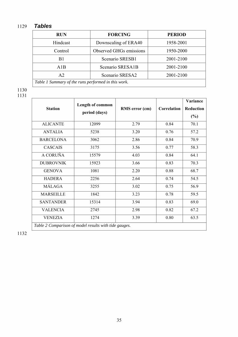
35
Tables 1129
RUN FORCING PERIOD
Hindcast Downscaling of ERA40 1958-2001
Control Observed GHGs emissions 1950-2000
B1 Scenario SRESB1 2001-2100
A1B Scenario SRESA1B 2001-2100
A2 Scenario SRESA2 2001-2100 Table 1 Summary of the runs performed in this work.
1130 1131
Station Length of common
period (days) RMS error (cm) Correlation
Variance
Reduction
(%)
ALICANTE 12099 2.79 0.84 70.1
ANTALIA 5238 3.20 0.76 57.2
BARCELONA 3062 2.86 0.84 70.9
CASCAIS 3175 3.56 0.77 58.3
A CORUÑA 15579 4.03 0.84 64.1
DUBROVNIK 15923 3.66 0.83 70.3
GENOVA 1081 2.20 0.88 68.7
HADERA 2256 2.64 0.74 54.5
MÁLAGA 3255 3.02 0.75 56.9
MARSEILLE 1842 3.23 0.78 59.5
SANTANDER 15314 3.94 0.83 69.0
VALENCIA 2745 2.98 0.82 67.2
VENEZIA 1274 3.39 0.80 63.5
Table 2 Comparison of model results with tide gauges.
1132
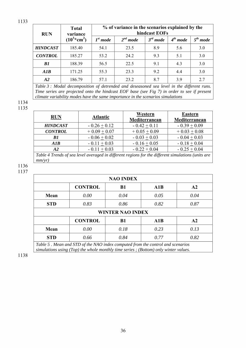
36
1133 % of variance in the scenarios explained by the
hindcast EOFs RUN Total
variance (103*cm2) 1st mode 2nd mode 3rd mode 4th mode 5th mode
HINDCAST 185.40 54.1 23.5 8.9 5.6 3.0
CONTROL 185.27 53.2 24.2 9.3 5.1 3.0
B1 188.39 56.5 22.5 9.1 4.3 3.0
A1B 171.25 55.3 23.3 9.2 4.4 3.0
A2 186.79 57.1 23.2 8.7 3.9 2.7
Table 3 : Modal decomposition of detrended and deseasoned sea level in the different runs. Time series are projected onto the hindcast EOF base (see Fig 7) in order to see if present climate variability modes have the same importance in the scenarios simulations 1134 1135
RUN Atlantic Western
Mediterranean Eastern
Mediterranean HINDCAST - 0.26 + 0.12 - 0.42 + 0.11 - 0.39 + 0.09 CONTROL + 0.09 + 0.07 + 0.05 + 0.09 + 0.03 + 0.08
B1 - 0.06 + 0.02 - 0.03 + 0.03 - 0.04 + 0.03 A1B - 0.11 + 0.03 - 0.16 + 0.05 - 0.18 + 0.04 A2 - 0.11 + 0.03 - 0.22 + 0.04 - 0.25 + 0.04
Table 4 Trends of sea level averaged in different regions for the different simulations (units are mm/yr) 1136 1137
NAO INDEX
CONTROL B1 A1B A2
Mean 0.00 0.04 0.05 0.04
STD 0.83 0.86 0.82 0.87
WINTER NAO INDEX
CONTROL B1 A1B A2
Mean 0.00 0.18 0.23 0.13
STD 0.66 0.84 0.77 0.82 Table 5 . Mean and STD of the NAO index computed from the control and scenarios simulations using (Top) the whole monthly time series ; (Bottom) only winter values. 1138
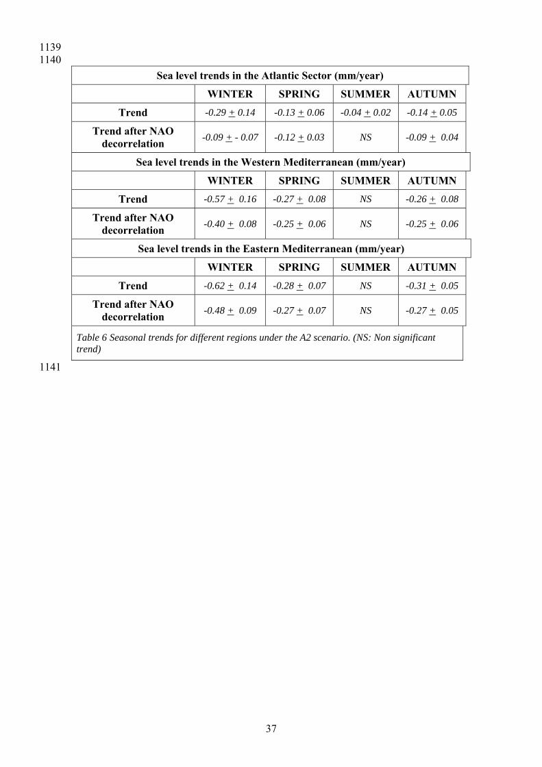
37
1139 1140
Sea level trends in the Atlantic Sector (mm/year)
WINTER SPRING SUMMER AUTUMN
Trend -0.29 + 0.14 -0.13 + 0.06 -0.04 + 0.02 -0.14 + 0.05
Trend after NAO decorrelation
-0.09 + - 0.07 -0.12 + 0.03 NS -0.09 + 0.04
Sea level trends in the Western Mediterranean (mm/year)
WINTER SPRING SUMMER AUTUMN
Trend -0.57 + 0.16 -0.27 + 0.08 NS -0.26 + 0.08
Trend after NAO decorrelation
-0.40 + 0.08 -0.25 + 0.06 NS -0.25 + 0.06
Sea level trends in the Eastern Mediterranean (mm/year)
WINTER SPRING SUMMER AUTUMN
Trend -0.62 + 0.14 -0.28 + 0.07 NS -0.31 + 0.05
Trend after NAO decorrelation
-0.48 + 0.09 -0.27 + 0.07 NS -0.27 + 0.05
Table 6 Seasonal trends for different regions under the A2 scenario. (NS: Non significant trend)
1141
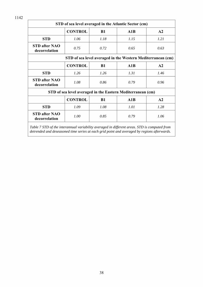
38
1142
STD of sea level averaged in the Atlantic Sector (cm)
CONTROL B1 A1B A2
STD 1.06 1.18 1.15 1.21
STD after NAO decorrelation
0.75 0.72 0.65 0.63
STD of sea level averaged in the Western Mediterranean (cm)
CONTROL B1 A1B A2
STD 1.26 1.26 1.31 1.46
STD after NAO decorrelation
1.08 0.86 0.79 0.96
STD of sea level averaged in the Eastern Mediterranean (cm)
CONTROL B1 A1B A2
STD 1.09 1.08 1.01 1.28
STD after NAO decorrelation
1.00 0.85 0.79 1.06
Table 7 STD of the interannual variability averaged in different areas. STD is computed from detrended and deseasoned time series at each grid point and averaged by regions afterwards.
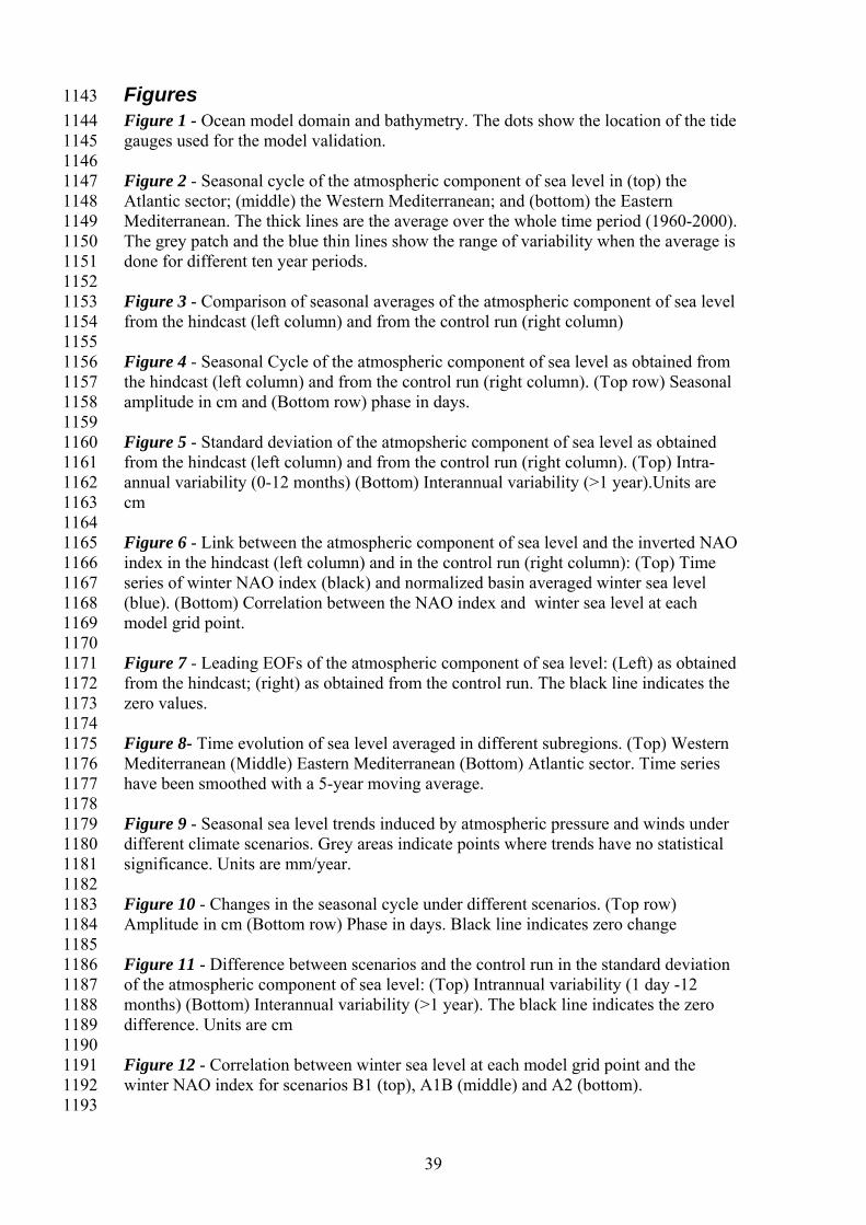
39
Figures 1143
Figure 1 - Ocean model domain and bathymetry. The dots show the location of the tide 1144 gauges used for the model validation. 1145 1146 Figure 2 - Seasonal cycle of the atmospheric component of sea level in (top) the 1147 Atlantic sector; (middle) the Western Mediterranean; and (bottom) the Eastern 1148 Mediterranean. The thick lines are the average over the whole time period (1960-2000). 1149 The grey patch and the blue thin lines show the range of variability when the average is 1150 done for different ten year periods. 1151 1152 Figure 3 - Comparison of seasonal averages of the atmospheric component of sea level 1153 from the hindcast (left column) and from the control run (right column) 1154 1155 Figure 4 - Seasonal Cycle of the atmospheric component of sea level as obtained from 1156 the hindcast (left column) and from the control run (right column). (Top row) Seasonal 1157 amplitude in cm and (Bottom row) phase in days. 1158 1159 Figure 5 - Standard deviation of the atmopsheric component of sea level as obtained 1160 from the hindcast (left column) and from the control run (right column). (Top) Intra-1161 annual variability (0-12 months) (Bottom) Interannual variability (>1 year).Units are 1162 cm 1163 1164 Figure 6 - Link between the atmospheric component of sea level and the inverted NAO 1165 index in the hindcast (left column) and in the control run (right column): (Top) Time 1166 series of winter NAO index (black) and normalized basin averaged winter sea level 1167 (blue). (Bottom) Correlation between the NAO index and winter sea level at each 1168 model grid point. 1169 1170 Figure 7 - Leading EOFs of the atmospheric component of sea level: (Left) as obtained 1171 from the hindcast; (right) as obtained from the control run. The black line indicates the 1172 zero values. 1173 1174 Figure 8- Time evolution of sea level averaged in different subregions. (Top) Western 1175 Mediterranean (Middle) Eastern Mediterranean (Bottom) Atlantic sector. Time series 1176 have been smoothed with a 5-year moving average. 1177 1178 Figure 9 - Seasonal sea level trends induced by atmospheric pressure and winds under 1179 different climate scenarios. Grey areas indicate points where trends have no statistical 1180 significance. Units are mm/year. 1181 1182 Figure 10 - Changes in the seasonal cycle under different scenarios. (Top row) 1183 Amplitude in cm (Bottom row) Phase in days. Black line indicates zero change 1184 1185 Figure 11 - Difference between scenarios and the control run in the standard deviation 1186 of the atmospheric component of sea level: (Top) Intrannual variability (1 day -12 1187 months) (Bottom) Interannual variability (>1 year). The black line indicates the zero 1188 difference. Units are cm 1189 1190 Figure 12 - Correlation between winter sea level at each model grid point and the 1191 winter NAO index for scenarios B1 (top), A1B (middle) and A2 (bottom). 1192 1193

40
Figure 13 - Time evolution of the seasonal cycle phase in a point located in the 1194 Levantine basin (blue line) and a point located in the Genoa Gulf (green line). (Top) 1195 control run, (bottom) A2 scenario. 1196 1197
41
1198
Fig 1. Ocean model domain and bathymetry. The dots show the location of the tide gauges used for the model validation.
1199 1200
Fig 2. Seasonal cycle of the atmospheric component of sea level in (top) the Atlantic sector; (middle) the Western Mediterranean; and (bottom) the Eastern Mediterranean. The thick lines are the average over the whole time period (1960-2000). The grey patch and the blue thin lines show the range of variability when the average is done for different ten year periods. 1201
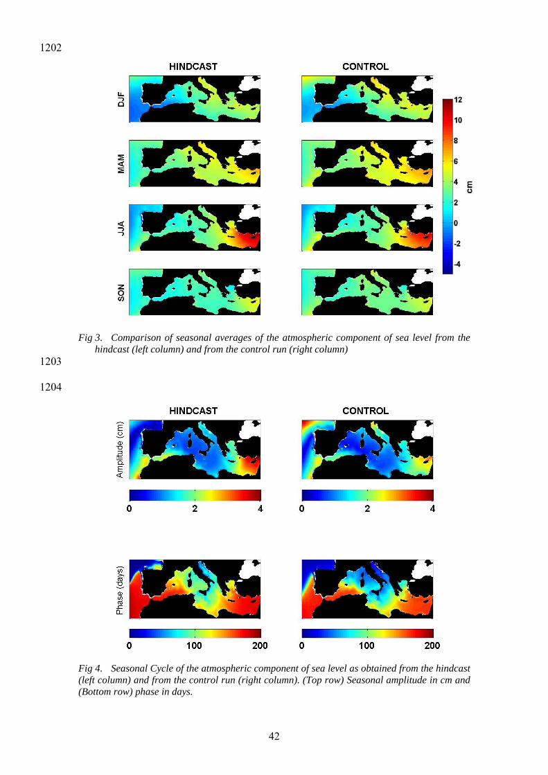
42
1202
Fig 3. Comparison of seasonal averages of the atmospheric component of sea level from the hindcast (left column) and from the control run (right column)
1203
1204
Fig 4. Seasonal Cycle of the atmospheric component of sea level as obtained from the hindcast (left column) and from the control run (right column). (Top row) Seasonal amplitude in cm and (Bottom row) phase in days.
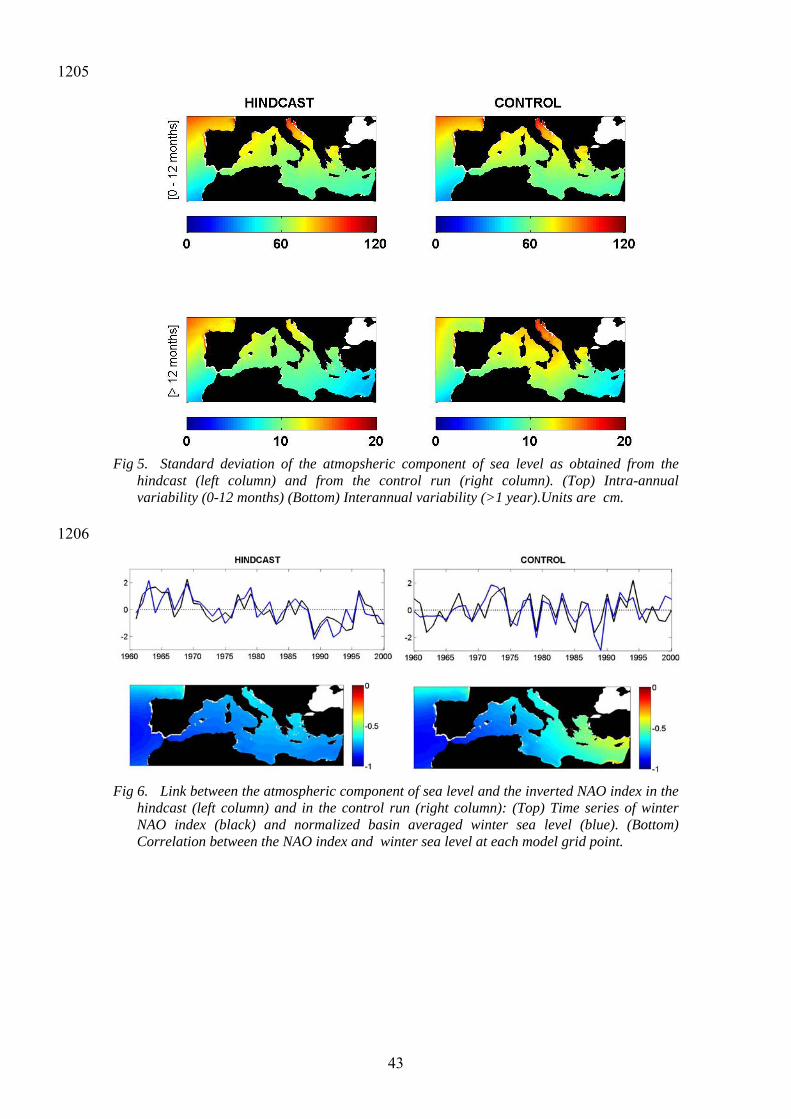
43
1205
Fig 5. Standard deviation of the atmopsheric component of sea level as obtained from the hindcast (left column) and from the control run (right column). (Top) Intra-annual variability (0-12 months) (Bottom) Interannual variability (>1 year).Units are cm.
1206
Fig 6. Link between the atmospheric component of sea level and the inverted NAO index in the hindcast (left column) and in the control run (right column): (Top) Time series of winter NAO index (black) and normalized basin averaged winter sea level (blue). (Bottom) Correlation between the NAO index and winter sea level at each model grid point.
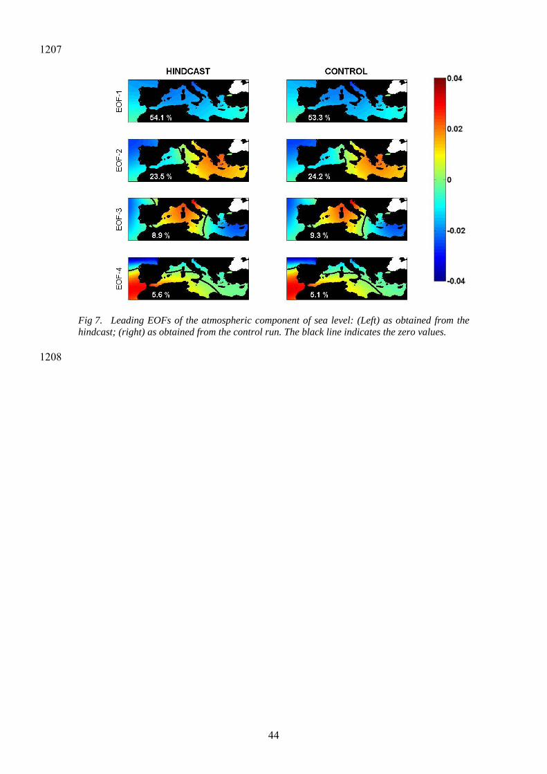
44
1207
Fig 7. Leading EOFs of the atmospheric component of sea level: (Left) as obtained from the hindcast; (right) as obtained from the control run. The black line indicates the zero values.
1208
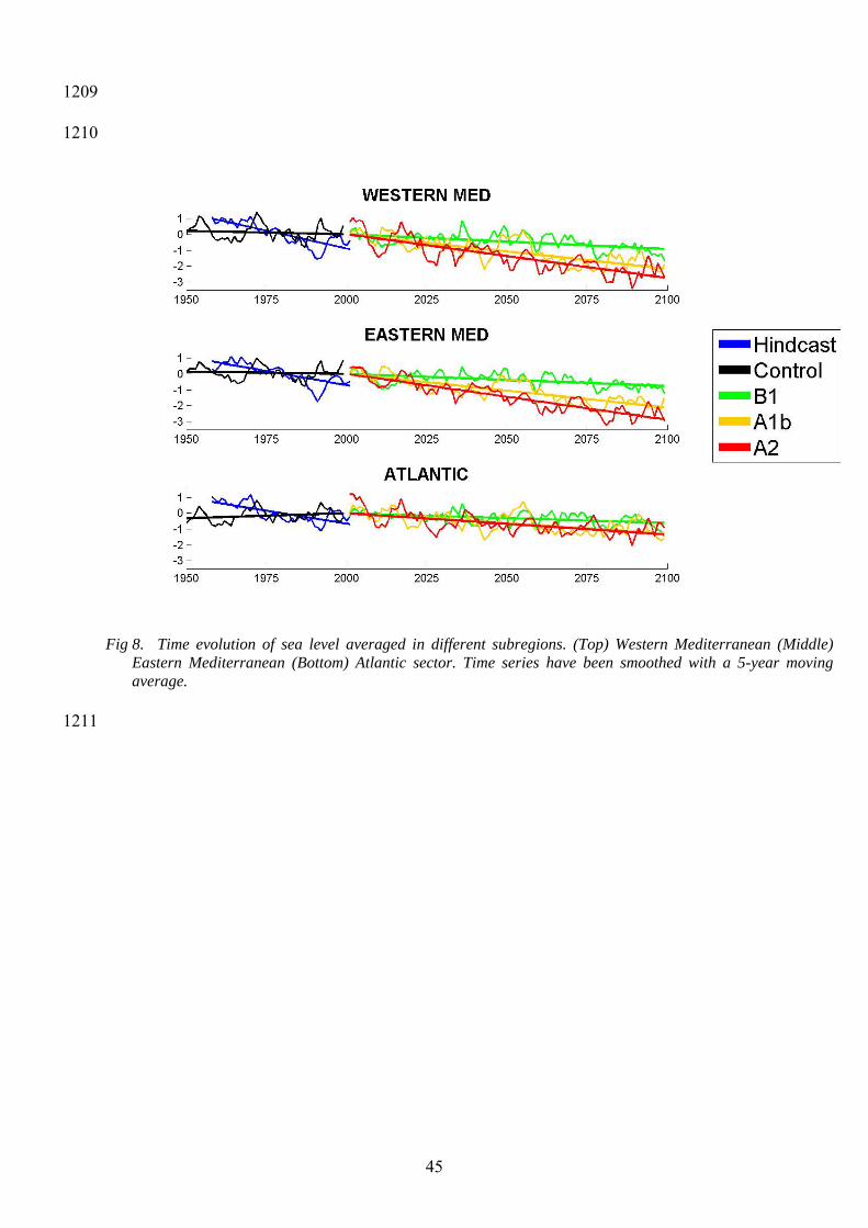
45
1209
1210
Fig 8. Time evolution of sea level averaged in different subregions. (Top) Western Mediterranean (Middle) Eastern Mediterranean (Bottom) Atlantic sector. Time series have been smoothed with a 5-year moving average.
1211
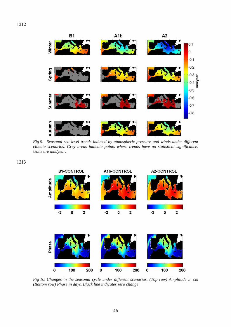
46
1212
Fig 9. Seasonal sea level trends induced by atmospheric pressure and winds under different climate scenarios. Grey areas indicate points where trends have no statistical significance. Units are mm/year.
1213
Fig 10. Changes in the seasonal cycle under different scenarios. (Top row) Amplitude in cm (Bottom row) Phase in days. Black line indicates zero change
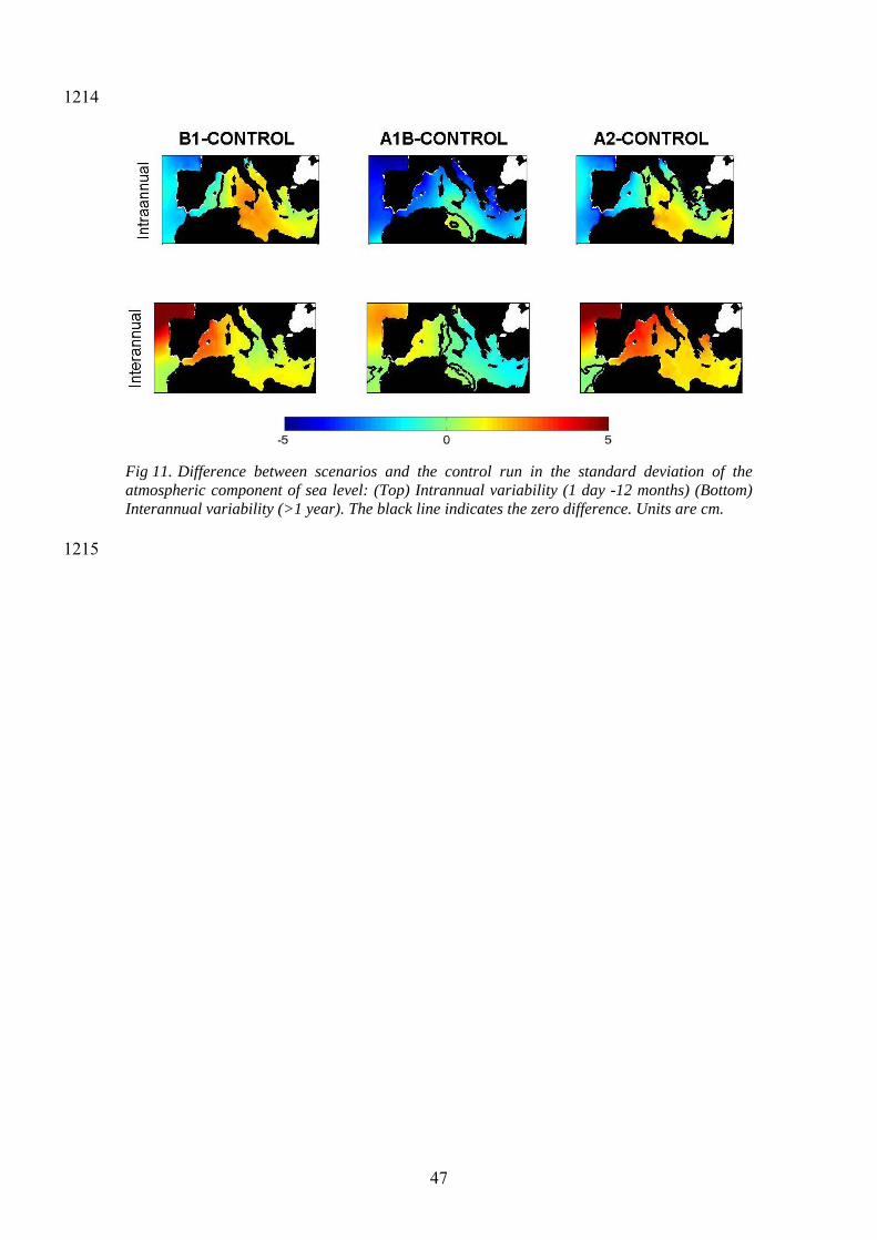
47
1214
Fig 11. Difference between scenarios and the control run in the standard deviation of the atmospheric component of sea level: (Top) Intrannual variability (1 day -12 months) (Bottom) Interannual variability (>1 year). The black line indicates the zero difference. Units are cm.
1215
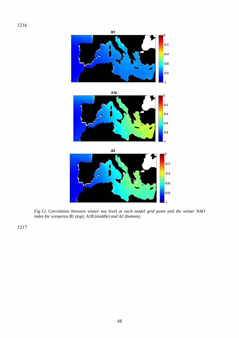
48
1216
Fig 12. Correlation between winter sea level at each model grid point and the winter NAO index for scenarios B1 (top), A1B (middle) and A2 (bottom).
1217
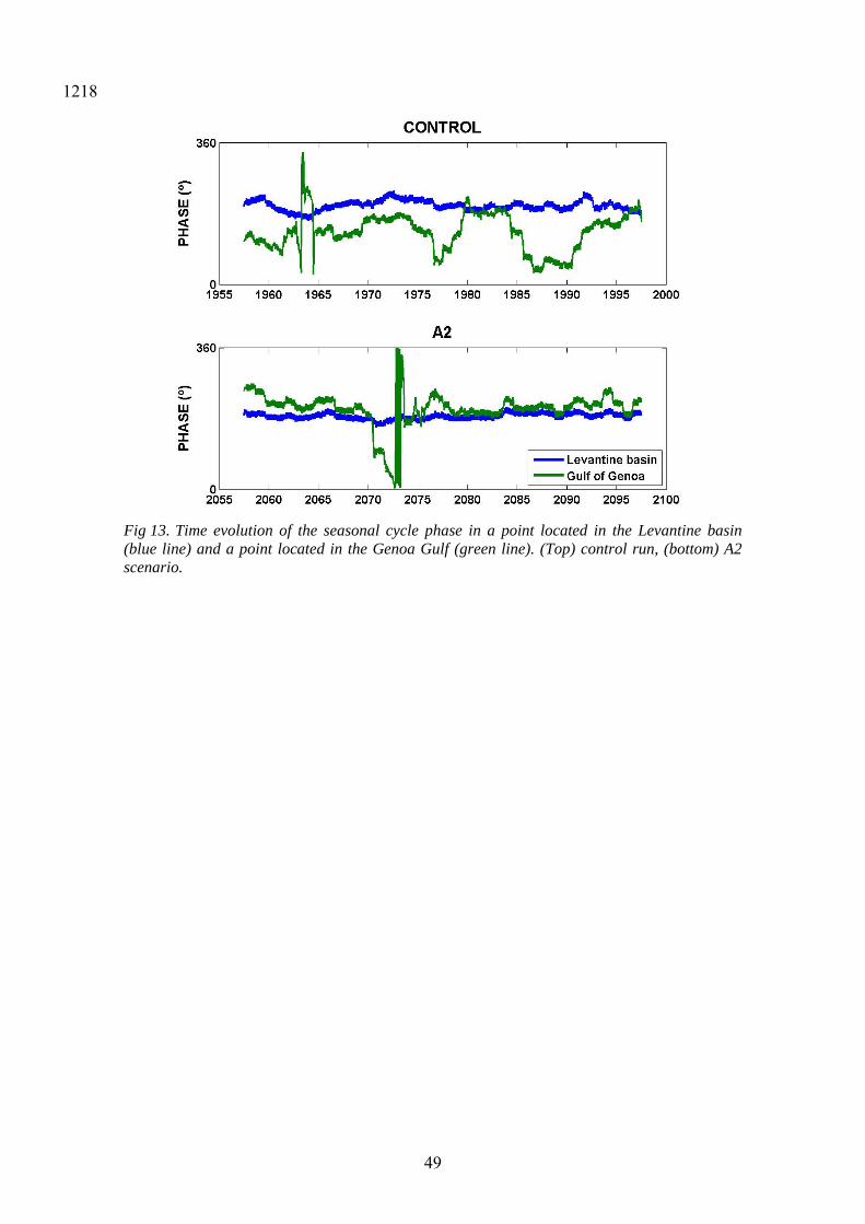
49
1218
Fig 13. Time evolution of the seasonal cycle phase in a point located in the Levantine basin (blue line) and a point located in the Genoa Gulf (green line). (Top) control run, (bottom) A2 scenario.

50
1219
Recommended