ORIGINAL PAPER
Automatic circle detection on digital images with an adaptivebacterial foraging algorithm
Sambarta Dasgupta • Swagatam Das •
Arijit Biswas • Ajith Abraham
Published online: 15 October 2009
� Springer-Verlag 2009
Abstract This article presents an algorithm for the
automatic detection of circular shapes from complicated
and noisy images without using the conventional Hough
transform methods. The proposed algorithm is based on a
recently developed swarm intelligence technique, known as
the bacterial foraging optimization (BFO). A new objective
function has been derived to measure the resemblance of a
candidate circle with an actual circle on the edge map of a
given image based on the difference of their center loca-
tions and radii lengths. Guided by the values of this
objective function (smaller means better), a set of encoded
candidate circles are evolved using the BFO algorithm so
that they can fit to the actual circles on the edge map of the
image. The proposed method is able to detect single or
multiple circles from a digital image through one shot of
optimization. Simulation results over several synthetic as
well as natural images with varying range of complexity
validate the efficacy of the proposed technique in terms of
its final accuracy, speed, and robustness.
Keywords Object recognition � Swarm intelligence �Bacterial foraging � Computer vision �Hand drawn shape location
1 Introduction
Past few decades have seen a massive growth in the field of
biologically inspired metaheuristics for search and opti-
mization. Computational cost having been reduced almost
dramatically; researchers from all corners are showing
more interest in following the underlying principles of
nature to solve nearly intractable optimization problems.
Following this tradition, practitioners in the field of
computer vision are also applying such metaheuristics to
difficult problems arising in the field. For example,
Wachowiak et al. (2004) applied the particle swarm opti-
mization (PSO) algorithm (Kennedy et al. 2001; Abraham
et al. 2006; Liu et al. 2007a, b), which draws inspiration
from the intelligent group behavior of social creatures, to
the problem of biomedical image registration. Le Hegarat-
Mascle et al. (2007) proposed a non-stationary Markov
model-based image regularization algorithm, which uses
another swarm intelligence algorithm known as ant colony
optimization (ACO) (Dorigo and Gambardella 1997).
De-Sian and Chien-Chang (2008) applied ACO for
improving the edge detection from digital images. Very
recently, Santamarıa et al. (2009) used memetic algorithms
(MAs) (Ong and Keane 2004) that are based on synergy of
evolutionary or any population-based approach with sepa-
rate individual learning or local improvement procedures,
in 3D Reconstruction of Forensic Objects.
Automatic identification and extraction of geometric
shapes from images are very useful in a number of tasks
because such shapes are often present in human-made
S. Dasgupta � S. Das � A. Biswas
Department of Electronics and Telecommunication Engineering,
Jadavpur University, Kolkata, India
e-mail: [email protected]
S. Das
e-mail: [email protected]
A. Biswas
e-mail: [email protected]
A. Abraham (&)
Machine Intelligence Research Labs (MIR Labs),
Scientific Network for Innovation and Research Excellence,
P.O. Box 2259, Auburn, WA 98071-2259, USA
e-mail: [email protected]
URL: http://www.mirlabs.org
123
Soft Comput (2010) 14:1151–1164
DOI 10.1007/s00500-009-0508-z
environments. They are also widely used as a part of man-
designed symbols. In particular, circle and ellipse detection
problems have been widely studied in the shape recogni-
tion community by using the deterministic techniques like
Hough transform (HT) (Illingworth and Kittler 1988;
Leavers 1993; Duda and Hart 1972), which often necessi-
tates high computation and storage requirements particu-
larly for high-dimensional applications. In order to
overcome these limitations, researchers have proposed new
approaches to HT, e.g., the probabilistic HT (Shaked et al.
1996), the randomized HT (Xu et al. 1990), and the fuzzy
HT (Han et al. 1993). Lam and Yuen (1996) came up with
a hybrid approach based on hypothesis filtering and HT to
detect circles. New integral transforms have also been
proposed in this context, e.g., see Becker et al. (2002). As
an alternative to the HT-based techniques, the shape rec-
ognition problem in computer vision has been handled with
stochastic search methods that include random sample
consensus (Fischer and Bolles 1981), simulated annealing
(SA) (Bongiovanni and Crescenzi 1995), and genetic
algorithm (GA) (Goldberg 1989). Stochastic algorithms
like GA exhibit adaptive and robust search behavior can
produce near optimal solutions very fast due to possessing
a large amount of implicit parallelism. However, they
cannot promise to achieve the solution every time.
Recently there has been a growing interest of researchers in
using GA for important shape detection tasks, e.g., Roth
and Levine (1994) proposed use of GA for primitive
extraction of images. Lutton et al. carried out a further
improvement of the aforementioned method recently in
2000 (Lutton and Martinez 1994). Yao et al. (2004) came
up with a multi-population GA to detect ellipses. Ayala-
Ramirez et al. (2006) presented a GA-based circle detector.
Their approach is capable of detecting multiple circles on
real images but fails frequently to detect small and
imperfect circles.
Passino (2002) proposed a powerful algorithm for real
parameter optimization, now known as the bacterial for-
aging optimization algorithm (BFOA) (Liu and Passino
2002). BFOA tries to mimic the individual and grouped
foraging behavior of Escherichia coli, a bacteria living in
our intestines. Until date the algorithm has found suc-
cessful applications in several real world problems like
optimal controller design (Liu and Passino 2002), harmonic
estimation (Mishra 2005), transmission loss reduction
(Tripathy et al. 2006), and power delay filter design
(Mishra and Bhende 2007; Das et al. 2009a, b; Kim et al.
2007; Biswas et al. 2007). This work presents an attempt to
detect circles (recognizing them by their shapes) from
digital images using an adaptive variant of the classical
BFOA. The work is not an extension of the HT techniques
described earlier and presents an altogether new approach
to this classical problem of computer vision. We use the
Canny edge detector (Canny 1986) to generate the edge-
map from a gray-scale image. The adaptive BFOA is then
applied to search the entire edge-map for circular shape.
Each bacterium here models a trial circle and an objective
function has been derived over the domain of such trial
circles in order to measure to what degree a trial circle
matches to an actual circle on the edge map of the image.
The better a test circle approximates the actual edge-circle,
the lesser becomes the value of this function. Minimization
of the objective function with BFOA ultimately leads to the
fast and robust extraction of circular shapes from the given
image. Comparison with one state-of-the-art GA-based
method and a randomized Hough transform (RHT) (Xu
et al. 1990) algorithm on multiple images indicate the
superiority of the proposed method.
The rest of the paper is organized as follows. In Sect. 2,
we provide a brief review of classical BFOA. In Sect. 3, we
derive the adaptation scheme of the chemotactic step in
BFOA leading to its faster convergence with a mathemat-
ical justification. Section 4 describes bacteria representa-
tion and also lays out the mathematical basis of the
objective function. Results of computer simulation over
several images have been presented in Sect. 5, and finally
the paper is concluded in Sect. 6 with a discussion of future
research directions.
2 The classical BFOA: an overview
Now suppose that we want to find the minimum of JðhÞwhere h 2 <p (i.e., h is a p-dimensional vector of real
numbers), and we do not have measurements or an ana-
lytical description of the gradient rJðhÞ: BFOA mimics
the four principal mechanisms observed in a real bacterial
system: chemotaxis, swarming, reproduction, and elimi-
nation-dispersal to solve this non-gradient optimization
problem. Below we introduce the formal notations used in
BFOA literature and then provide the complete pseudo-
code of the BFO algorithm. A more detailed description of
the steps of BFOA is out of the scope of this paper and can
be found in Passino (2002), Liu and Passino (2002) and
Dasgupta et al. (2008).
Let us define a chemotactic step to be a tumble followed
by a tumble or a tumble followed by a run. Let j be the
index for the chemotactic step. Let k be the index for the
reproduction step. Let l be the index of the elimination-
dispersal event. Also let
p Dimension of the search space,
S Total number of bacteria in the population,
Nc The number of chemotactic steps,
Ns The swimming length
Nre The number of reproduction steps,
1152 S. Dasgupta et al.
123
Ned The number of elimination-dispersal events,
Ped Elimination-dispersal probability,
C (i) The size of the step taken in the random direction
specified by the tumble.
Let Pðj; k; lÞ ¼ fhiðj; k; lÞji ¼ 1; 2; . . .; Sg represent the
position of each member in the population of the S bac-
teria at the jth chemotactic step, kth reproduction step,
and lth elimination-dispersal event. Here, let Jði; j; k; lÞdenote the cost at the location of the ith bacterium
hiðj; k; lÞ 2 <p (sometimes, we drop the indices and refer
to the ith bacterium position as hi). Note that we will
interchangeably refer to J as being a ‘‘cost’’ (using ter-
minology from optimization theory) and as being a
nutrient surface (in reference to the biological connec-
tions). For actual bacterial populations, S can be very
large (e.g., S = 109), but p = 3. In our computer simu-
lations, we will use much smaller population sizes and
will keep the population size fixed. BFOA, however,
allows p [ 3 so that we can apply the method to higher
dimensional optimization problems. Below, we briefly
describe the four prime steps in BFOA. We also provide a
pseudo-code of the complete algorithm.
1. Chemotaxis This process simulates the movement of
an E. coli cell through swimming and tumbling via
flagella. Suppose hiðj; k; lÞ represents ith bacterium at
jth chemotactic, kth reproductive and lth elimination-
dispersal step. CðiÞ is a scalar and indicates the size of
the step taken in the random direction specified by the
tumble (run length unit). Then in computational
chemotaxis, the movement of the bacterium may be
represented by
hiðjþ 1; k; lÞ ¼ hiðj; k; lÞ þ CðiÞ DðiÞffiffiffiffiffiffiffiffiffiffiffiffiffiffiffiffiffiffiffi
DTðiÞDðiÞq ; ð1Þ
where D indicates a unit length vector in the random
direction.
2. Swarming An interesting group behavior has been
observed for several motile species of bacteria includ-
ing E. coli and S. typhimurium, where stable spatio-
temporal patterns (swarms) are formed in semisolid
nutrient medium. A group of E. coli cells arrange
themselves in a traveling ring by moving up the
nutrient gradient when placed amidst a semisolid
matrix with a single nutrient chemo-effecter. The cells
when stimulated by a high level of succinate, release
an attractant aspartate, which helps them to aggregate
into groups and thus move as concentric patterns of
swarms with high bacterial density. The cell-to-cell
signaling in E. coli swarm may be represented by the
following function.
Jccðh;Pðj; k; lÞÞ ¼X
S
i¼1
Jccðh; hiðj; k; lÞÞ
¼X
S
i¼1
�dattractant exp �wattractant
X
p
m¼1
ðhm � himÞ
2
!" #
þX
S
i¼1
hrepellant exp �wrepellant
X
p
m¼1
ðhm � himÞ
2
!" #
;
ð2Þ
where Jccðh;Pðj; k; lÞÞ is the objective function value to
be added to the actual objective function (to be mini-
mized) to present a time varying objective function.
The coefficients daatractant;wattractant; hrepellant; and
wrepellant control the strength of the cell-to-cell signal-
ing. More specifically daatractant is the depth of the
attractant released by the cell, wattractant is a measure of
the width of the attractant signal (a quantification of the
diffusion rate of the chemical), hrepellant ¼ dattractant is
the height of the repellant effect (a bacterium cell also
repels a nearby cell in the sense that it consumes nearby
nutrients and it is not physically possible to have two
cells at the same location), and wrepellant is a measure of
the width of the repellant. For a detailed discussion on
the function Jcc please see, Passino (2002) and Liu and
Passino (2002).
3. Reproduction The least healthy bacteria eventually die
while each of the healthier bacteria (those yielding
lower value of the objective function) asexually split
into two bacteria, which are then placed in the same
location. This keeps the swarm size constant.
4. Elimination and dispersal To simulate this phenome-
non in BFOA some bacteria are liquidated at random
with a very small probability while the new replace-
ments are randomly initialized over the search space.
3 A simple adaptation scheme for chemotactic step
of the BFOA
3.1 Mathematical foundation
Let us consider a single bacterium cell that undergoes
chemotactic steps according to (1) over a one-dimensional
objective function. The bacterium lives in continuous time
and at the tth instant its position is given by hðtÞ: Below we
list a few assumptions that are considered for the sake of
gaining mathematical insight.
1. The objective function JðhÞ is continuous and differ-
entiable at all points in the search space.
2. The chemotactic step size C is not very large.
Automatic circle detection on digital images 1153
123
3. The analysis applies to the regions of the fitness
landscape where gradients of the function are small,
i.e., near to the optima.
Let, at time t position of an individual bacterium be hand value of objective function (to be minimized) be JðhÞ:Also assume that, after a very small time interval Dt; its
position changes by an amount Dh: Then the new value of
the objective function becomes Jðhþ DhÞ: According to
the chemotactic step used in BFOA, the bacterium changes
its position only if the modified objective function value is
less than the previous one, i.e., JðhÞ[ Jðhþ DhÞ, i.e.,
JðhÞ � Jðhþ DhÞ is positive, i.e.,JðhÞ�JðhþDhÞ
Dt is positive.
(As time is unidirectional, Dt is a positive infinitesimally
small quantity. So, sign of any number is retained after it is
divided by Dt:)
The decision-making (i.e., whether to take a step or not)
activity of the bacterium can be modeled by a unit step
function uðxÞ as,
uJðhÞ � Jðhþ DhÞ
Dt
� �
¼ 1; ifJðhÞ � Jðhþ DhÞ
Dt[ 0;
¼ 0; otherwise:
Thus,
DhDt¼ u
JðhÞ � Jðhþ DhÞDt
� �
CD; ð3Þ
where C indicates the chemotactic step height and Dindicates the direction of tumble (here it can assume only
two values 1 or -1 with uniform probabilities). Note that
modeling the decision-making activity of a bacterium with
unit step function reinforce the local search behavior since
a step is taken only if it keeps on minimizing (i.e.,
improving the fitness of a bacterium) following the
directives of original BFOA. In that case, the
advancement is done with an intensity C in D direction.
Here, we have assumed in unit time bacterium takes a
chemotactic step. DhDt is the velocity.
) DhDt¼ u �Jðhþ DhÞ � JðhÞ
Dt
� �
CD:
Now velocity of the bacterium is given by,
Vb ¼ LtDt!0
DhDt
¼ u � LtDh!0
Jðhþ DhÞ � JðhÞDh
� �
LtDt!0
DhDt
� �
CD; ð4Þ
) Vb ¼ h0 ¼ u �dJðhÞ
dhdhdt
� �
CD;
) Vb ¼ uð�GVbÞCD; ð5Þ
where G = J0(h) = gradient of the objective function at h.
Since the unit step function uðxÞ has a jump discontinuity at
x ¼ 0; to simplify the analysis further, we replace uðxÞ with
the continuous logistic function /ðxÞ (Anwal 1998), where
/ðxÞ ¼ 1
1þ e�kx: ð6Þ
We note that, uðxÞ ¼ Ltk!1 /ðxÞ ¼ Ltk!11
1þe�kx
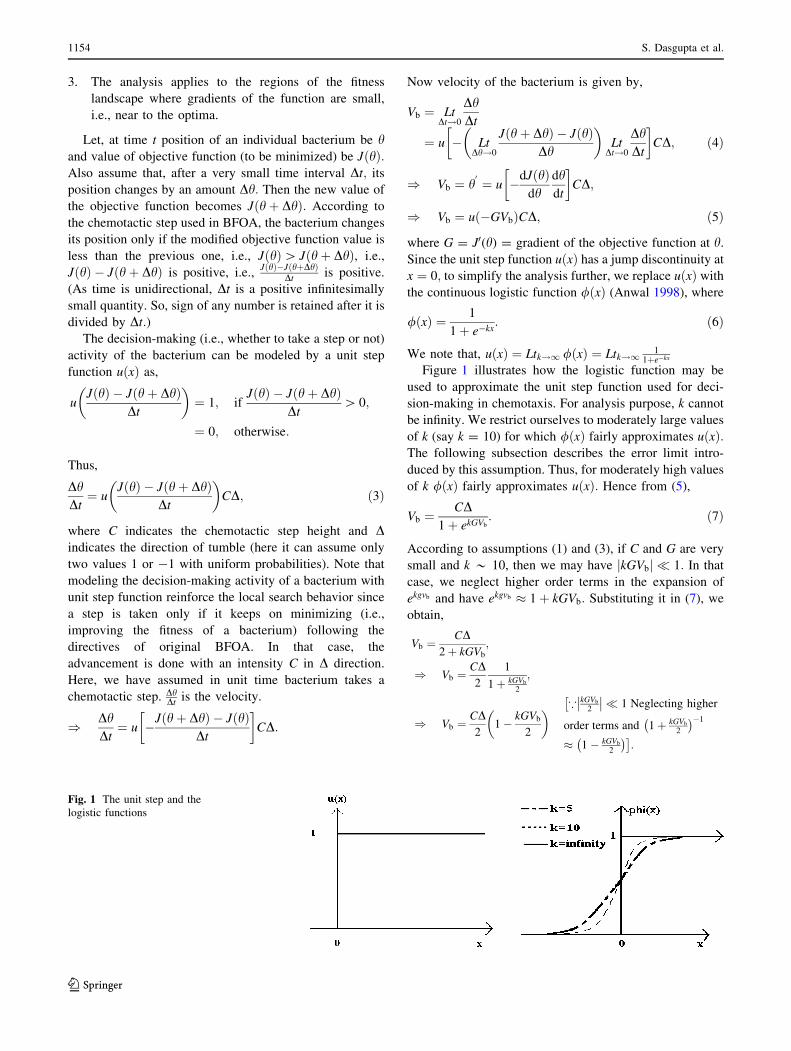
Figure 1 illustrates how the logistic function may be
used to approximate the unit step function used for deci-
sion-making in chemotaxis. For analysis purpose, k cannot
be infinity. We restrict ourselves to moderately large values
of k (say k = 10) for which /ðxÞ fairly approximates uðxÞ:The following subsection describes the error limit intro-
duced by this assumption. Thus, for moderately high values
of k /ðxÞ fairly approximates uðxÞ: Hence from (5),
Vb ¼CD
1þ ekGVb: ð7Þ
According to assumptions (1) and (3), if C and G are very
small and k * 10, then we may have jkGVbj � 1: In that
case, we neglect higher order terms in the expansion of
ekgvb and have ekgvb � 1þ kGVb: Substituting it in (7), we
obtain,
Vb ¼CD
2þ kGVb
;
) Vb ¼CD2
1
1þ kGVb
2
;
) Vb ¼CD2
1� kGVb
2
� �
*kGVb
2
�
�
�
�� 1 Neglecting higher�
order terms and 1þ kGVb
2
�1
� 1� kGVb
2
�
:
Fig. 1 The unit step and the
logistic functions
1154 S. Dasgupta et al.
123
After some manipulation we have,
Vb ¼2CD
4þ kGCDð8Þ
) Vb ¼CD2
1
1þ kCGD4
;
) Vb ¼CD2
1� kGCD4
� �
*kGCD
4
�
�
�
�� 1; as Dj j ¼ 1 and�
neglecting the higher order terms�;
) Vb ¼ �kC2
8Gþ CD
2; ð9Þ
) dhdt¼ �aGþ b; ð10Þ
where a is �kC2
8and b is CD
2:
The classical gradient descent algorithm (CGDA)
(Fletcher 1987) is given by the following dynamics in
single dimension:
dhdt¼ �aG; ð11Þ
where a is the learning rate.
Similarity between Eqs. 9, 10, and 11 suggests that
chemotaxis is a modified CGDA where a; which is a
function of chemotactic step size, can be identified as the
learning rate of chemotaxis.
3.2 Oscillation problem: need for adaptive chemotaxis
If magnitude of the gradient decreases consistently, near
the optima or very close to the optima a of Eq. 15 becomes
comparable to b: Then gradually b becomes dominant.
When Gj j ! 0; dhdt
�
�
�
� � bj j ¼ CD2
�
�
�
� ¼ C2½* Dj j ¼ 1�:Let us
assume the bacterium has reached close to the optimum.
But as we have derived dhdt
�
�
�
� ¼ C2; the bacterium does not
stop taking chemotactic steps. It oscillates about the
optima. This crisis can be remedied if step size C is made
adaptive according to the following relation,
C ¼ wjJðhÞjjJðhÞj þ k
¼ w
1þ k=JðhÞj j: ð12Þ
Here, k and w ([1) are positive constants. Thus from (12),
we see, if JðhÞ ! 0; then C ! 0: Therefore, there would
be no oscillation if the bacterium reaches optima. The
functional form of (12) causes C to vanish near the optima.
Besides, it plays another important role described below.
From (12), we have, when JðhÞ is large kjJðhÞj ! 0 and
consequently C ! wð[ 1Þ: This has an important physical
significance. If magnitude of cost function is large for an
individual bacterium, it is in vicinity of the noxious sub-
stance. It will then try to move to a place with better
nutrient concentration by taking large steps. On the other
hand, the bacterium when in nutrient rich zone, i.e., with
small magnitude of the objective function value, tries to
retain its position. Naturally, its step size becomes small.
Dasgupta et al. (2008) have illustrated the effectiveness of
the above-mentioned adaptation scheme over several
numerical benchmarks.
4 The ABFOA-based circle detection algorithm
4.1 The scheme for population initialization
An individual member of the population of sample circles
is actually a trial solution. Each sample circle is repre-
sented as a bacterial position h~¼ ½x0; y0; r0�T; where first
two components of the vector are x and y co-ordinates of
the center of that circle and third term stands for the radius.
Let ðxk; yk; rkÞ be the kth test circle in the population,
where k ¼ 1; . . .; S; S is the population size, i.e., it denotes
total number of test circles. In initialization phase, random
values within suitable range are assigned to each of the
three entries of the vectors. Two statistical properties of
sample points on a candidate circle are used in this regard,
where one property is used to find a suitable value for co-
ordinates of probable center of the test circle and, another
is used to model its probable radius. These two properties
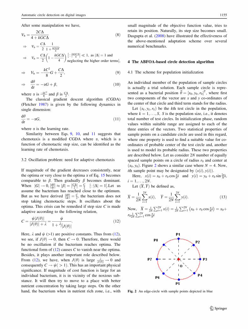
are described below. Let us consider 2N number of equally
spaced sample points on a circle of radius r0 and center at
ðx0; y0Þ: Figure 2 shows a similar case where N ¼ 4: Now,
ith sample point may be designated by ðxðiÞ; yðiÞÞ:Here, xðiÞ ¼ x0 þ r0 cos p
Ni and yðiÞ ¼ y0 þ r0 sin 2pN i;
i ¼ 1; . . .; 2N:
Let ðX; YÞ be defined as,
X ¼ 1
2N
X
2N
i¼1
xðiÞ; Y ¼ 1
2N
X
2N
i¼1
yðiÞ: ð13Þ
Now, X ¼ 12N
P2Ni¼1 xðiÞ ¼ 1
2N
P2Ni¼1 x0 þ r0 cos p
Ni
¼ x0þr0
12N
P2Ni¼1 cos p
Ni
Fig. 2 An edge-circle with sample points depicted in blue
Automatic circle detection on digital images 1155
123
)X ¼ x0 þ r0
sin psin p
2N
cospð2nþ 1Þ
4n) X ¼ x0
* sin p ¼ 0½ �:
Similarly, we can show that Y ¼ y0:
)X ¼ x0; Y ¼ y0: ð14Þ
Let us also define
r ¼
ffiffiffiffiffiffiffiffiffiffiffiffiffiffiffiffiffiffiffiffiffiffiffiffiffiffiffiffiffiffiffiffiffiffiffiffiffiffiffiffiffiffiffiffiffiffiffiffiffiffiffiffiffiffiffiffiffiffiffiffiffiffiffiffiffiffiffiffiffiffiffi
1
2N
X
2N
i¼1
ðxðiÞ � XÞ2 þ ðyðiÞ � YÞ2 !
v
u
u
t ; ð15Þ
) r2 ¼ 1
2N
X
2N
i¼1
ðxðiÞ � x0Þ2 þ ðyðiÞ � y0Þ2 !
;
½*X ¼ x0; Y ¼ y0�;
) r2 ¼ 1
2N
X
2N
i¼1
r0 cospN
i� 2
þ r0 sinpN
i� 2
!
) r2 ¼ r20
1
2N
X
2N
i¼1
cospN
i� 2
þ sinpN
i� 2
!
;
) r2 ¼ r20;
) r2 ¼ r20 : ð16Þ
To initialize kth test-circle we form a set of 2mk edge-
points drawn at random from the edge-map, where 2mk ¼randðL;UÞ such that L;U specify upper and lower limit of
2mk: Let ðxðiÞ; yðiÞÞ be the ith edge-point, i ¼ 1; . . .; 2mk
and ðxk; yk; rkÞ denotes the kth test circle to be initialized.
Now, we assign values to three entries of the vector taking
guidelines of Eqs. 13 and 15.We assign
xk ¼1
2mk
X
2mk
i¼1
xðiÞ; yk ¼1
2mk
X
2mk
i¼1
yðiÞ
and rk ¼
ffiffiffiffiffiffiffiffiffiffiffiffiffiffiffiffiffiffiffiffiffiffiffiffiffiffiffiffiffiffiffiffiffiffiffiffiffiffiffiffiffiffiffiffiffiffiffiffiffiffiffiffiffiffiffiffiffiffiffiffiffiffiffiffiffiffiffiffiffiffiffiffiffiffi
1
2mk
X
2mk
i¼1
ðxðiÞ � xkÞ2 þ ðyðiÞ � ykÞ2 !
v
u
u
t :
This initialization scheme is adopted with the expectation
that the selected edge points may lie on the actual circle or
very close to it, so that we may reach a good approximation
of the center and radius.
4.2 The objective function
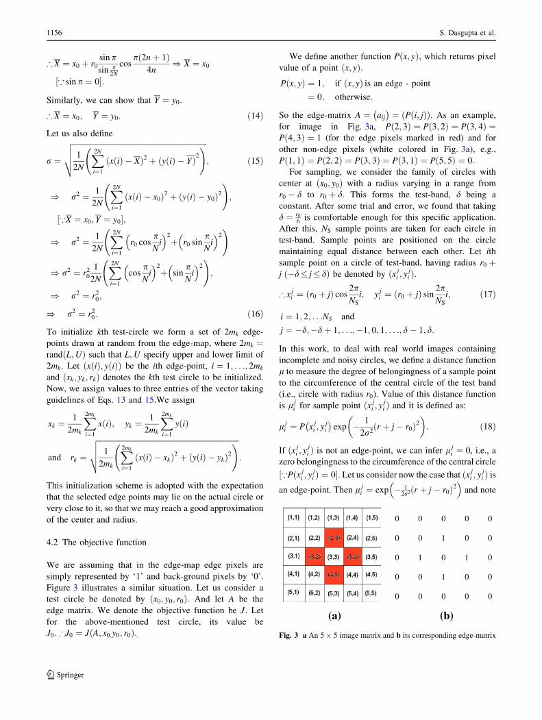
We are assuming that in the edge-map edge pixels are
simply represented by ‘1’ and back-ground pixels by ‘0’.
Figure 3 illustrates a similar situation. Let us consider a
test circle be denoted by ðx0; y0; r0Þ: And let A be the
edge matrix. We denote the objective function be J: Let
for the above-mentioned test circle, its value be
J0: )J0 ¼ JðA; x0;y0; r0Þ:.
We define another function Pðx; yÞ; which returns pixel
value of a point ðx; yÞ:Pðx; yÞ ¼ 1; if ðx; yÞ is an edge - point
¼ 0; otherwise:
So the edge-matrix A ¼ aij
¼ Pði; jÞð Þ: As an example,
for image in Fig. 3a, Pð2; 3Þ ¼ Pð3; 2Þ ¼ Pð3; 4Þ ¼Pð4; 3Þ ¼ 1 (for the edge pixels marked in red) and for
other non-edge pixels (white colored in Fig. 3a), e.g.,
Pð1; 1Þ ¼ Pð2; 2Þ ¼ Pð3; 3Þ ¼ Pð3; 1Þ ¼ Pð5; 5Þ ¼ 0:
For sampling, we consider the family of circles with
center at ðx0; y0Þ with a radius varying in a range from
r0 � d to r0 þ d: This forms the test-band, d being a
constant. After some trial and error, we found that taking
d ¼ r0
6is comfortable enough for this specific application.
After this, NS sample points are taken for each circle in
test-band. Sample points are positioned on the circle
maintaining equal distance between each other. Let ith
sample point on a circle of test-band, having radius r0 þj ð�d� j� dÞ be denoted by ðx j
i ; yji Þ:
) x ji ¼ ðr0 þ jÞ cos
2pNS
i; y ji ¼ ðr0 þ jÞ sin
2pNS
i; ð17Þ
i ¼ 1; 2; . . .NS and
j ¼ �d;�dþ 1; . . .;�1; 0; 1; . . .; d� 1; d:
In this work, to deal with real world images containing
incomplete and noisy circles, we define a distance function
l to measure the degree of belongingness of a sample point
to the circumference of the central circle of the test band
(i.e., circle with radius r0). Value of this distance function
is l ji for sample point ðx j
i ; yji Þ and it is defined as:
l ji ¼ P x j
i ; yji
exp � 1
2r2ðr þ j� r0Þ2
� �
: ð18Þ
If ðx ji ; y
ji Þ is not an edge-point, we can infer l j
i ¼ 0, i.e., a
zero belongingness to the circumference of the central circle
½*Pðx ji ; y
ji Þ ¼ 0�: Let us consider now the case that ðx j
i ; yji Þ is
an edge-point. Then l ji ¼ exp � 1
2r2ðr þ j� r0Þ2�
and note
00000
00100
01010
00100
00000
(a) (b)
Fig. 3 a An 5� 5 image matrix and b its corresponding edge-matrix
1156 S. Dasgupta et al.
123
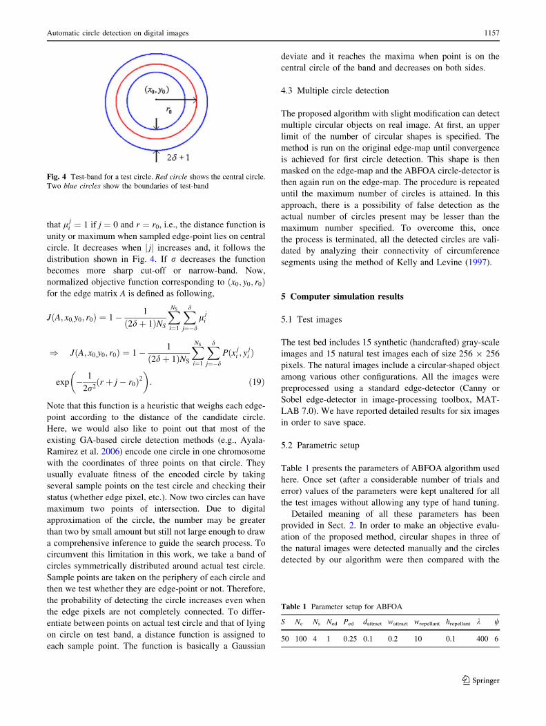
that l ji ¼ 1 if j ¼ 0 and r ¼ r0, i.e., the distance function is
unity or maximum when sampled edge-point lies on central
circle. It decreases when jj j increases and, it follows the
distribution shown in Fig. 4. If r decreases the function
becomes more sharp cut-off or narrow-band. Now,
normalized objective function corresponding to ðx0; y0; r0Þfor the edge matrix A is defined as following,
JðA; x0;y0; r0Þ ¼ 1� 1
ð2dþ 1ÞNS
X
NS
i¼1
X
d
j¼�d
l ji
) JðA; x0;y0; r0Þ ¼ 1� 1
ð2dþ 1ÞNS
X
NS
i¼1
X
d
j¼�d
Pðx ji ; y
ji Þ
exp � 1
2r2ðr þ j� r0Þ2
� �
: ð19Þ
Note that this function is a heuristic that weighs each edge-
point according to the distance of the candidate circle.
Here, we would also like to point out that most of the
existing GA-based circle detection methods (e.g., Ayala-
Ramirez et al. 2006) encode one circle in one chromosome
with the coordinates of three points on that circle. They
usually evaluate fitness of the encoded circle by taking
several sample points on the test circle and checking their
status (whether edge pixel, etc.). Now two circles can have
maximum two points of intersection. Due to digital
approximation of the circle, the number may be greater
than two by small amount but still not large enough to draw
a comprehensive inference to guide the search process. To
circumvent this limitation in this work, we take a band of
circles symmetrically distributed around actual test circle.
Sample points are taken on the periphery of each circle and
then we test whether they are edge-point or not. Therefore,
the probability of detecting the circle increases even when
the edge pixels are not completely connected. To differ-
entiate between points on actual test circle and that of lying
on circle on test band, a distance function is assigned to
each sample point. The function is basically a Gaussian
deviate and it reaches the maxima when point is on the
central circle of the band and decreases on both sides.
4.3 Multiple circle detection
The proposed algorithm with slight modification can detect
multiple circular objects on real image. At first, an upper
limit of the number of circular shapes is specified. The
method is run on the original edge-map until convergence
is achieved for first circle detection. This shape is then
masked on the edge-map and the ABFOA circle-detector is
then again run on the edge-map. The procedure is repeated
until the maximum number of circles is attained. In this
approach, there is a possibility of false detection as the
actual number of circles present may be lesser than the
maximum number specified. To overcome this, once
the process is terminated, all the detected circles are vali-
dated by analyzing their connectivity of circumference
segments using the method of Kelly and Levine (1997).
5 Computer simulation results
5.1 Test images
The test bed includes 15 synthetic (handcrafted) gray-scale
images and 15 natural test images each of size 256 9 256
pixels. The natural images include a circular-shaped object
among various other configurations. All the images were
preprocessed using a standard edge-detector (Canny or
Sobel edge-detector in image-processing toolbox, MAT-
LAB 7.0). We have reported detailed results for six images
in order to save space.
5.2 Parametric setup
Table 1 presents the parameters of ABFOA algorithm used
here. Once set (after a considerable number of trials and
error) values of the parameters were kept unaltered for all
the test images without allowing any type of hand tuning.
Detailed meaning of all these parameters has been
provided in Sect. 2. In order to make an objective evalu-
ation of the proposed method, circular shapes in three of
the natural images were detected manually and the circles
detected by our algorithm were then compared with the
Fig. 4 Test-band for a test circle. Red circle shows the central circle.
Two blue circles show the boundaries of test-band
Table 1 Parameter setup for ABFOA
S Nc Ns Ned Ped dattract wattract wrepellant hrepellant k w
50 100 4 1 0.25 0.1 0.2 10 0.1 400 6
Automatic circle detection on digital images 1157
123
hand-label ones (considered as the ground truth images)
using a new heuristic score.
For the GA algorithm described in Ayala-Ramirez et al.
(2006), we take the population size = 70, crossover
probability = 0.55, mutation probability = 0.10, number
of elite individuals = 2. We also took as selection method,
the roulette wheel selection and as a crossover method, the
1-point crossover. The parametric setup appears as the best
set, configured by Ayala-Ramirez et al. (2006) after lot of
hand tuning experiments. The same fitness function as the
one described by Ayala-Ramirez et al. (2006) has been
used for the GA implementation.
5.3 Error score and success rate
To test accuracy of the algorithm obtained result is com-
pared with ground truth. First, the circle in the edge-map is
detected manually and it is referred as the ground-truth
image. Next three peripheral points are taken on the
manually detected circle. We know that through three non-
collinear points only one circle can pass. So from previous
three points, we get integer-approximated (as we are
dealing with digital circle) center and radius of the ground-
truth circle (GTC). Let center of the GTC be ðxGTC; yGTCÞand its radius be rGTC: Let the chosen points on the GTC be
ðx1; y1Þ; ðx2; y2Þ; and ðx3; y3Þ:Then
xGTC ¼
x22 þ y2
2 � ðx21 þ y2
1Þ 2ðy2 � y1Þx2
3 þ y23 � ðx2
1 þ y21Þ 2ðy3 � y1Þ
�
�
�
�
�
�
�
�
�
�
4ðx2 � x1Þðy3 � y1Þ � ðx3 � x1Þðy2 � y1Þ
and yGTC ¼
2ðx2 � x1Þ x22 þ y2
2 � ðx21 þ y2
1Þ2ðx3 � x1Þ x2
3 þ y23 � ðx2
1 þ y21Þ
�
�
�
�
�
�
�
�
�
�
4ðx2 � x1Þðy3 � y1Þ � ðx3 � x1Þðy2 � y1Þ:
If center and radius of the detected circle found by
algorithm is denoted by ðxD; yDÞ and rD; then we can define
an error score in the following way,
ES ¼ gð xGTC � xDj j þ ðyGTC � yDj jÞ þ l rGTC � rDj j ð20Þ
First term represents shift of center of the detected circle
from that of GTC and second term signifies difference of
their radii. g and l are two weights associated with each
term in (20). They may be chosen according to the accu-
racy required. We have taken g ¼ 0:05 and l ¼ 0:1: This
particular choice of parameters ensures that radii difference
gets priority to the difference of the centers of the manually
detected circle and the machine-detected circle. Here we
assume that if ES is found to be less than 1, then the
algorithm gets a success, otherwise, we say that it has
failed to detect the edge-circle. Note that for g ¼ 0:05 and
l ¼ 0:1; ES \ 1 means the maximum difference of radius
tolerated is 10 while the maximum mismatch in the
location of the center can be 20 (in number of pixels). From
this consideration, success rate (SR) is defined as per-
centage of reaching success in certain number of trials.
5.4 Simulation strategy
The algorithm has been developed from scratch on a
Pentium IV 2.4 GHz PC using C language under windows
XP environment. Fifty independent runs of the proposed
algorithm were carried out with different seeds of random
number generator over each test image.
5.5 Presentation of results
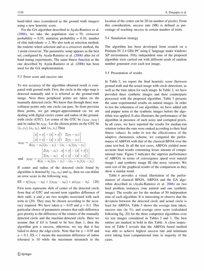
In Table 2, we report the final heuristic score (between
ground truth and the actual image with circle detection), as
well as the time taken for each image. In Table 2, we have
provided three synthetic images and their counterparts
processed with the proposed algorithm. Table 3 presents
the same experimental results on natural images. In order
to test the robustness of our algorithm, we have added salt
and pepper noise to the synthetic images before the algo-
rithm was applied. It also illustrates the performance of the
algorithm in presence of such noisy and corrupted pixels.
In all cases, we have reported the results for median-run
solution (when the runs were ranked according to their final
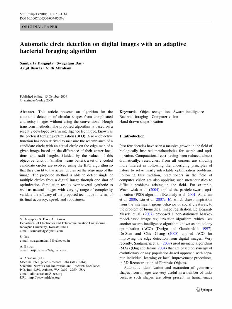
fitness values). In order to test the effectiveness of the
adaptive chemotaxis scheme, we compared the perfor-
mance of ABFOA with that of the classical BFOA over the
same test-bed. In all the test cases, ABFOA yielded more
accurate final results consuming lesser amount of compu-
tational time. Figure 5 indicates the superior performance
of ABFOA in terms of convergence speed over natural
image 1 and synthetic image III (the noisy version). We
omit rest of the graphical results of the comparison as they
show a similar trend.
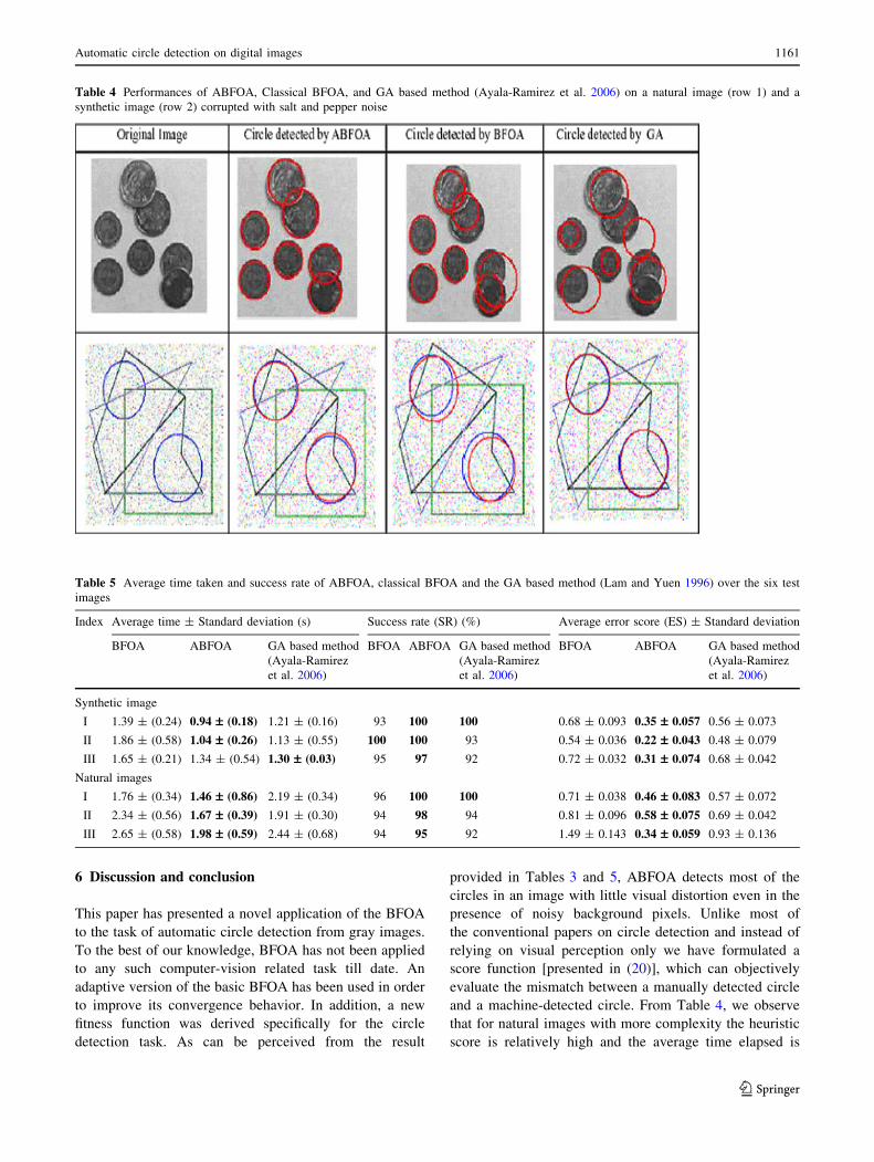
Table 4 provides a visual illustration of the perfor-
mances of classical BFOA, ABFOA and the GA algo-
rithm described in (Ayala-Ramirez et al. 2006) on two
hard problem instances (one natural and one synthetic
image). The results are for the median of 50 independent
runs of each algorithm. It is interesting to observe that the
deviation between the detected circle and actual circle is
least for ABFOA. Table 5 shows the average time taken,
success rate (in %), and average error score (calculated
following Eq. 20) for the three competitor algorithms over
six test images considered in Tables 2 and 3. The best
entries are marked in bold in this Table. A close inspec-
tion of Table 5 reveals that the ABFOA based method
was able to achieve highest success rate and minimum
error taking least computational time in majority of the
cases.
1158 S. Dasgupta et al.
123
A non-parametric statistical significance test called
Wilcoxon’s rank sum test for independent samples
(Wilcoxon 1945; Garcıa et al. 2008) has been conducted
at the 5% significance level on the error score (ES) data
of Table 5. Table 6 shows reports the P-values produced
by Wilcoxon’s rank sum test for comparison of the error
scores of two groups (one group corresponding to AB-
FOA and the other corresponding to a competitor algo-
rithm) at a time. As a null hypothesis, it is assumed that
there is no significant difference between the mean val-
ues of two groups. Whereas, the alternative hypothesis is
that there is significant difference in the mean values of
the two groups. All the P values reported in the Table
are less than 0.05 (5% significance level). This is strong
evidence against the null hypothesis, indicating that the
better mean values of the performance metrics produced
by ABFO is statistically significant and has not occurred
by chance.
Table 7 demonstrates relative performance of ABFOA
in comparison to the RHT algorithm described in Ong and
Keane (2004). Images taken for the test are complicated
and also comprises of different geometrical figures. RHT
finds out the circle located in the figures satisfactorily but
ABFOA is found to determine the position of circles with
higher accuracy. Table 8 reports the corresponding average
time taken, success rate (in %), and average error score
(calculated following Eq. 20) for ABFOA and RHT algo-
rithms over three test images considered in Table 7.
Table 2 Synthetic images and detected circles
Automatic circle detection on digital images 1159
123
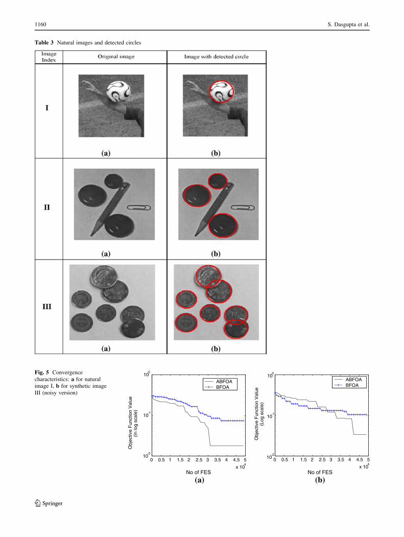
Table 3 Natural images and detected circles
0 0.5 1 1.5 2 2.5 3 3.5 4 4.5 510
-2
10-1
100
No of FES
Obj
ectiv
e F
unct
ion
Val
ue(I
n lo
g sc
ale)
ABFOABFOA
x 104
Obj
ectiv
e F
unct
ion
Val
ue(L
og s
cale
)
(a) (b)
0 0.5 1 1.5 2 2.5 3 3.5 4 4.5 5
No of FESx 10
4
10-2
10-1
100
ABFOABFOA
Fig. 5 Convergence
characteristics: a for natural
image I, b for synthetic image
III (noisy version)
1160 S. Dasgupta et al.
123
6 Discussion and conclusion
This paper has presented a novel application of the BFOA
to the task of automatic circle detection from gray images.
To the best of our knowledge, BFOA has not been applied
to any such computer-vision related task till date. An
adaptive version of the basic BFOA has been used in order
to improve its convergence behavior. In addition, a new
fitness function was derived specifically for the circle
detection task. As can be perceived from the result
provided in Tables 3 and 5, ABFOA detects most of the
circles in an image with little visual distortion even in the
presence of noisy background pixels. Unlike most of
the conventional papers on circle detection and instead of
relying on visual perception only we have formulated a
score function [presented in (20)], which can objectively
evaluate the mismatch between a manually detected circle
and a machine-detected circle. From Table 4, we observe
that for natural images with more complexity the heuristic
score is relatively high and the average time elapsed is
Table 4 Performances of ABFOA, Classical BFOA, and GA based method (Ayala-Ramirez et al. 2006) on a natural image (row 1) and a
synthetic image (row 2) corrupted with salt and pepper noise
Table 5 Average time taken and success rate of ABFOA, classical BFOA and the GA based method (Lam and Yuen 1996) over the six test
images
Index Average time ± Standard deviation (s) Success rate (SR) (%) Average error score (ES) ± Standard deviation
BFOA ABFOA GA based method
(Ayala-Ramirez
et al. 2006)
BFOA ABFOA GA based method
(Ayala-Ramirez
et al. 2006)
BFOA ABFOA GA based method
(Ayala-Ramirez
et al. 2006)
Synthetic image
I 1.39 ± (0.24) 0.94 – (0.18) 1.21 ± (0.16) 93 100 100 0.68 ± 0.093 0.35 – 0.057 0.56 ± 0.073
II 1.86 ± (0.58) 1.04 – (0.26) 1.13 ± (0.55) 100 100 93 0.54 ± 0.036 0.22 – 0.043 0.48 ± 0.079
III 1.65 ± (0.21) 1.34 ± (0.54) 1.30 – (0.03) 95 97 92 0.72 ± 0.032 0.31 – 0.074 0.68 ± 0.042
Natural images
I 1.76 ± (0.34) 1.46 – (0.86) 2.19 ± (0.34) 96 100 100 0.71 ± 0.038 0.46 – 0.083 0.57 ± 0.072
II 2.34 ± (0.56) 1.67 – (0.39) 1.91 ± (0.30) 94 98 94 0.81 ± 0.096 0.58 – 0.075 0.69 ± 0.042
III 2.65 ± (0.58) 1.98 – (0.59) 2.44 ± (0.68) 94 95 92 1.49 ± 0.143 0.34 – 0.059 0.93 ± 0.136
Automatic circle detection on digital images 1161
123
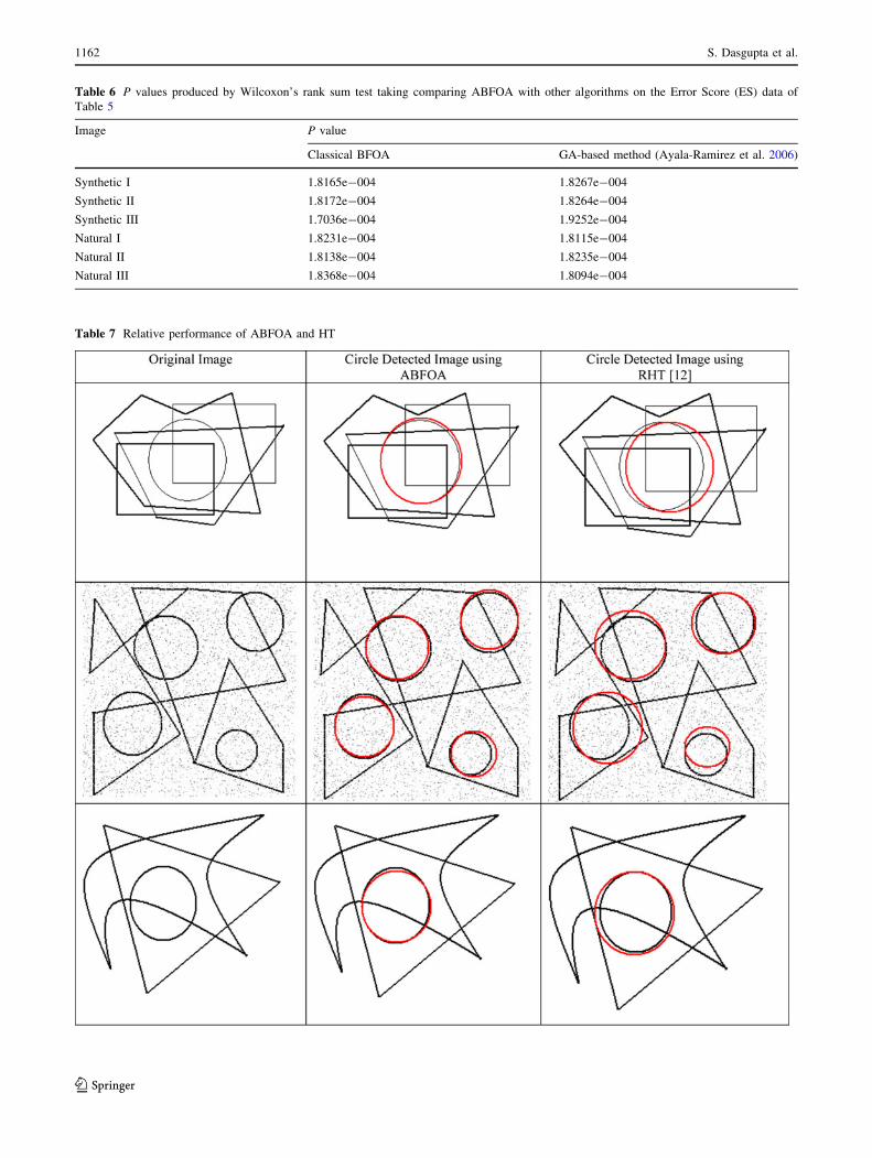
Table 6 P values produced by Wilcoxon’s rank sum test taking comparing ABFOA with other algorithms on the Error Score (ES) data of
Table 5
Image P value
Classical BFOA GA-based method (Ayala-Ramirez et al. 2006)
Synthetic I 1.8165e-004 1.8267e-004
Synthetic II 1.8172e-004 1.8264e-004
Synthetic III 1.7036e-004 1.9252e-004
Natural I 1.8231e-004 1.8115e-004
Natural II 1.8138e-004 1.8235e-004
Natural III 1.8368e-004 1.8094e-004
Table 7 Relative performance of ABFOA and HT
1162 S. Dasgupta et al.
123
higher as well. Through the use of non-parametric Wilco-
xon’s rank sum test, we demonstrated that the ABFOA-
based method could outperform both GA (as described in
Ayala-Ramirez et al. 2006) and classical BFOA in a sta-
tistically significant fashion. Since both classical BFOA
and ABFOA use the same initial population, bacteria rep-
resentation scheme and fitness function, it is evident that
the superior performance of ABFOA is attributed to its
adaptation scheme of the chemotactic step-size C.
Although Table 7 indicated that ABFOA can yield
better results on complicated and noisy images as com-
pared to the RHT, note that the objective of our paper is not
to devise a circle-detection algorithm that could beat all the
HT based methods discovered earlier, but to show that a
new swarm intelligence algorithm called BFOA with the
suggested modifications can serve as an attractive alterna-
tive of the GA that has been used earlier to extract circular
shapes from objects successfully. This way, the work
undertaken here, encourages further research on the
application of BFOA to the tasks related to shape extrac-
tion in computer vision. Future research will focus on
hybridizing ABFOA with different HT based techniques
for automatic shape extraction. In addition, application of
the ABFOA based techniques for automatic shape recog-
nition by mobile robots may also be studied. In future, we
shall also attempt to compare the performance of our
ABFOA based algorithm with other evolutionary compu-
tation techniques on the circle detection problem
quantitatively.
References
Abraham A, Guo H, Liu H (2006) Swarm intelligence: foundations,
perspectives and applications, swarm intelligent systems. In:
Nedjah N, Mourelle L (eds) Studies in computational intelli-
gence. Springer, Germany, pp 3–25
Anwal RP (1998) Generalized functions: theory and technique, 2nd
edn. Birkhauser, Boston
Ayala-Ramirez V, Garcia-Capulin CH, Perez-Garcia A, Sanchez-
Yanez RE (2006) Circle detection on images using genetic
algorithms. Pattern Recogn Lett 27:652–657
Becker J, Grousson S, Coltuc D (2002) From Hough transforms to
integral transforms. In: Proceedings of international geoscience
and remote sensing symposium, IGARSS_02 3:1444–1446
Biswas A, Dasgupta S, Das S, Abraham A (2007) A synergy of
differential evolution and bacterial foraging algorithm for global
optimization. Neural Netw World 17(6):607–626
Bongiovanni G, Crescenzi P (1995) Parallel simulated annealing for
shape detection. Comput Vision Image Understanding 61(1):60–69
Canny J (1986) A computational approach to edge detection. IEEE
Trans Pattern Anal Mach Intell 8:679–714
Das S, Biswas A, Dasgupta S, Abraham A (2009a) Bacterial foraging
optimization algorithm: theoretical foundations, analysis, and
applications, foundations of computational intelligence. Global
optimization, studies in computational intelligence, vol 3.
Springer, Germany, pp 23–55. ISBN: 978-3-642-01084-2
Das S, Dasgupta S, Biswas A, Abraham A, Konar A (2009b) On
stability of the chemotactic dynamics in bacterial foraging
optimization algorithm. IEEE Trans Syst Man Cybern Part A
39(3):670–679
Dasgupta S, Das S, Abraham A, Biswas A (2009) Adaptive
computational chemotaxis in bacterial foraging optimization:
an analysis. IEEE Trans Evol Comput 13(4):919–941
De-Sian L, Chien-Chang C (2008) Edge detection improvement by
ant colony optimization. Pattern Recogn Lett 29(4):416–425
Dorigo M, Gambardella LM (1997) Ant colony system: a cooperative
learning approach to the traveling salesman problem. IEEE
Trans Evol Comput 1(1):53–66
Duda RO, Hart PE (1972) Use of the Hough transformation to detect
lines and curves in pictures. Comm Assoc Comput Mach 15:11–15
Fischer M, Bolles R (1981) Random sample consensus: a paradigm to
model fitting with applications to image analysis and automated
cartography. CACM 24(6):381–395
Fletcher R (1987) Practical methods of optimization, 2nd edn. Wiley,
Chichester
Garcıa S, Molina D, Lozano M, Herrera F (2008) A study on the use
of non-parametric tests for analyzing the evolutionary algo-
rithms’ behaviour: a case study on the CEC’2005 Special session
on real parameter optimization. J Heurist. doi:10.1007/s10732-
008-9080-4
Goldberg DE (1989) Genetic algorithms in search. Optimization and
machine learning. Kluwer, Boston
Han JH, Koczy LT, Poston T (1993) Fuzzy Hough transform. In:
Proceedings 2nd international conference on fuzzy systems
2:803–808
Illingworth J, Kittler J (1988) Survey: a survey of the Hough
transform. Comput Vision Graphics Image Process 44:87–116
Kelly M, Levine M (1997) Advances in image understanding. Finding
and describing objects in complex images. IEEE Computer
Society Press, pp 209–225
Kennedy J, Eberhart R, Shi Y (2001) Swarm intelligence. Morgan
Kaufmann Academic Press, Menlo Park
Kim DH, Abraham A, Cho JH (2007) Hybrid genetic algorithm and
bacterial foraging approach for global optimization. Inf Sci
177(18):3918–3937
Lam W, Yuen S (1996) Efficient techniques for circle detection using
hypothesis filtering and Hough transform. IEEE Proc Visual
Image Signal Process 143(5):292–300
Table 8 Average time taken and success rate of ABFOA and HT over the 3 test images
Index Average time ± Standard deviation (s) Success rate (SR) (%) Average Error Score (ES) ± Standard deviation
ABFOA HT based method
(Xu et al. 1990)
ABFOA HT based method
(Xu et al. 1990)
ABFOA HT based method
(Xu et al. 1990)
I 1.24 – (0.36) 1.81 ± (0.28) 94 91 0.68 – 0.088 0.74 ± 0.096
II 2.82 – (0.45) 3.01 ± (0.55) 90 86 0.92 – 0.087 1.12 ± 0.132
III 2.65 ± (0.46) 1.60 – (0..53) 94 90 0.56 – 0.069 0.47 ± 0.078
Automatic circle detection on digital images 1163
123
Le Hegarat-Mascle S, Hegarat-Mascle L, Kallel A, Descombes X
(2007) Ant colony optimization for image regularization based
on a nonstationary markov modeling. IEEE Trans Image Process
16(3):865–878
Leavers VF (1993) Survey: which Hough transforms. CVGIP Image
Understanding 58:250–264
Liu Y, Passino KM (2002) Biomimicry of social foraging bacteria for
distributed optimization: models, principles, and emergent
behaviors. J Optim Theory Appl 115(3):603–628
Liu H, Abraham A, Clerc M (2007a) Chaotic dynamic characteristics
in swarm intelligence. Appl Soft Comput J 7(3):1019–1026
Liu H, Abraham A, Zhang W (2007b) A fuzzy adaptive turbulent
particle swarm optimization. Int J Innov Comput Appl 1(1):39–47
Lutton E, Martinez P (1994) A genetic algorithm for the detection
2-D geometric primitives on images. In: Proceedings of the
12th international conference on pattern recognition (ICPR_94),
vol 1, Jerusalem, Israel, pp 526–528
Mishra S (2005) A hybrid least square-fuzzy bacterial foraging
strategy for harmonic estimation. IEEE Trans Evol Comput
9(1):61–73
Mishra S, Bhende CN (2007) Bacterial Foraging Technique-Based
Optimized Active Power Filter for Load Compensation. IEEE
Trans Power Deliv 22(1):457–465
Ong YS, Keane AJ (2004) Meta-Lamarckian learning in memetic
algorithms. IEEE Trans Evol Comput 8:99–110
Passino KM (2002) Biomimicry of bacterial foraging for distributed
optimization and control. IEEE Control Systems Magazine, pp
52–67
Roth G, Levine MD (1994) Geometric primitive extraction using a
genetic algorithm. IEEE Trans Pattern Anal Mach Intell
16(9):901–905
Santamarıa J, Cordon O, Damas S, Garcıa-Torres JM, Quirin A
(2009) Performance evaluation of memetic approaches in 3D
reconstruction of forensic objects. Soft Comput 13(8–9):883–
904
Shaked D, Yaron O, Kiryati N (1996) Deriving stopping rules for the
probabilistic Hough transform by sequential analysis. Computer
Vision Image Understanding 63:512–526
Tripathy M, Mishra S, Lai LL, Zhang QP (2006) Transmission loss
reduction based on FACTS and bacteria foraging algorithm.
PPSN, pp 222–231
Wachowiak MP, Smolikova R, Yufeng Z, Zurada JM, Elmaghraby
AS (2004) An approach to multimodal biomedical image
registration utilizing particle swarm optimization. IEEE Trans
Evol Comput 8(3):289–301
Wilcoxon F (1945) Individual comparisons by ranking methods.
Biometrics 1:80–83
Xu L, Oja E, Kultanen P (1990) A new curve detection method:
Randomized Hough Transform (RHT). Pattern Recogn Lett
11(5):331–338
Yao J, Kharma N, Grogono P (2004) Fast robust GA-based ellipse
detection. In: Proceedings of 17th international conference on
pattern recognition ICPR-04, vol 2, Cambridge, UK, pp 859–862
1164 S. Dasgupta et al.
123
Recommended