Finance and Economics Discussion SeriesDivisions of Research & Statistics and Monetary Affairs
Federal Reserve Board, Washington, D.C.
Banks as Regulated Traders
Antonio Falato, Diana Iercosan, and Filip Zikes
2019-005
Please cite this paper as:Falato, Antonio, Diana Iercosan, and Filip Zikes (2021). “Banks as Regulated Traders,”Finance and Economics Discussion Series 2019-005r1. Washington: Board of Governors ofthe Federal Reserve System, https://doi.org/10.17016/FEDS.2019.005r1.
NOTE: Staff working papers in the Finance and Economics Discussion Series (FEDS) are preliminarymaterials circulated to stimulate discussion and critical comment. The analysis and conclusions set forthare those of the authors and do not indicate concurrence by other members of the research staff or theBoard of Governors. References in publications to the Finance and Economics Discussion Series (other thanacknowledgement) should be cleared with the author(s) to protect the tentative character of these papers.
Banks as Regulated Traders
Antonio Falato Diana Iercosan Filip Zikes∗
July 29, 2021
Abstract
Banks use trading as a vehicle to take risk. Using unique high-frequency regulatorydata, we estimate the sensitivity of weekly bank trading profits to aggregate equity,fixed-income, credit, currency and commodity risk factors. Our estimates imply thatU.S. banks had large trading exposures to equity market risk before the Volcker Rule,which they curtailed afterwards. They also have exposures to credit and currency risk.The results hold up in a quasi-natural experimental design that exploits the phased-inintroduction of reporting requirements to address identification. Heterogeneity andplacebo tests further corroborate the results. Counterfactual stress-test analyses quan-tify the financial stability implications.
∗Falato, [email protected], Division of Financial Stability, Federal Reserve Board; Iercosan,[email protected], Division of Supervision and Regulation, Federal Reserve Board; Zikes,[email protected], Division of Financial Stability, Federal Reserve Board. We are grateful to SirioAramonte, Juliane Begenau (discussant), Darrell Duffie, Andrea Eisfeldt, Mark Flannery (discussant), Jean-Sebastian Fontaine, Michael Gordy, David Lynch, David McArthur, Bernadette Minton (discussant), Ric-cardo Rebonato, Jason Schmidt, Anjan Thakor, Greg Udell, Skander Van den Heuvel, conference participantsat the AFA Annual Meetings, the NBER Corporate Finance, the Annual FDIC Bank Research Conference,and seminar participants at the Federal Reserve Board, New York Fed, SEC, CFTC, and QuantMind foruseful comments, suggestions, or help with data. Matthew Carl, Jacob Faber, Alex Jiron, and Maddie Whiteprovided excellent research assistance. The views expressed in this paper are those of the authors and shouldnot be interpreted as representing the views of the Federal Reserve Board or any other person associatedwith the Federal Reserve System.
1 Introduction
Trading has become an important part of the business model of the modern banking corpo-
ration.1 With the traditional loan-centric model of banking in steady decline over the last
two decades, the trading book has become the main alternative to loans along with securities
holding. In the late 1990s and early 2000s, loans accounted for over 60% of aggregate total
assets in the U.S. banking sector and trading assets were less than 1/10 the size of loans.
By contrast, loans accounted for as little as 40% of total assets over the last decade, while
securities holding was about 18%, and trading assets stood as high as 13%, totaling more
than the aggregate value of tier 1 capital. Of course, the experience of the financial crisis
serves as a harsh reminder that massive trading book losses can have a systemic impact.
And bank trading remains at the center of the financial regulation agenda, with recent ef-
forts underway to streamline the regulation of trading that was enacted under the broader
framework of the Dodd-Frank Act (see Squam Lake Group, 2010; Greenwood et al. 2017a,b;
Quarles, 2018 for the academic and policy debate on financial regulation). Yet, despite its
importance, there has been little systematic study of the trading book in banking, with the
literature having focused on more traditional assets and on the liabilities side of the bank
balance sheet.2
In order to fill the gap in the banking literature, we use newly-available high-frequency
regulatory data on the daily trading book profits and losses of U.S. banks. Trading is
a powerful instrument for hedging risk, but it also allows banks to quickly and cheaply
take speculative risk. If banks use trading to increase risk, then individual banks may be
vulnerable to potentially large losses.3 If all banks take similar positions, the entire banking
1Several recent reports by government agencies and central banks have been devoted to the bank tradingbook. For example, the Federal Reserve Board’s Iercosan et al. (2017a,b,c) examine trading activities at U.S.systemically important banks post crisis. The BIS published a policy paper in 2013 on the Basel Committee’sfundamental review of trading book capital requirements (https://www.bis.org/publ/bcbs265.pdf). And theECB has recently increased scrutiny of the trading book of the euro zone’s biggest lenders reportedly due tofinancial stability concerns (Bloomberg Business, June 13, 2018).
2For recent exceptions, see Hanson, Shleifer, Stein, and Vishny (2015) and recent work by Minton,Stulz, and Taboada (2017), who conjecture that trading assets can explain important features of bankvaluation, such as the cross-sectional negative relation between bank valuation and size. Outside of banking,an influential intermediary-based asset pricing literature emphasizes the central role of banks as marginalinvestors to explain risk premiums in asset markets (see He and Krishnamurthy (2018) for a survey).
3In fact, trading losses tend to account for a large fraction of total losses projected under the severelyadverse scenario in the results of the Federal Reserve’s annual stress tests of U.S. banks since 2009.
1
sector may be vulnerable. To determine the risk exposures of banks via trading, we build on
the standard approach in banking (Flannery and James (1984), Gorton and Rosen (1995))
and infer the direction of trading from bank trading profits. We estimate the sensitivity
of banks’ net trading profits to a broad array of aggregate risk factors, including equity
markets and interest rates. We use our estimates as a key input to quantify bank trading
risk exposures and empirically address two main questions: first, does trading increase or
decrease systemic risk in the U.S. banking sector, in the sense of exposure to aggregate risk
factors? Second, is government regulation of bank trading effective at curtailing risk?
At the end of 2017, trading assets in the U.S. banking sector stood at over 10 percent of
total assets, a decline relative to the pre-crisis peak of 17 percent but still quadrupled relative
to the early 1990s. Moreover, trading is concentrated within a relatively small number of
big banks, with the six largest banks holding more than three quarters of the total trading
assets of the banking sector and trading constituting almost 20 percent of total assets for
these large banks. Because of their size and concentration, as well as the large trading
losses in the financial crisis, bank trading activities have been at the center of the regulatory
agenda over the last decade. The so called ”Volcker Rule” was finalized in 2013 with the aim
to mitigate risk taking by federally insured banks through a ban on proprietary trading.4
The intended goal was to prevent banks from holding assets that increase the likelihood of
incurring a substantial loss or pose a threat to financial stability, which is in line with the
theory of bank regulation (Koehn and Santomero, 1980; Kim and Santomero, 1988). Assets
held for prudent market making, underwriting, or hedging, are allowed, while those held to
take directional positions aimed at profiting from price changes are not allowed. The rule
relies on the supervisory process to identify prohibited assets by requiring that the agencies
tasked with enforcement regularly monitor quantitative risk metrics, such as aggregate risk
factor sensitivities. In summary, theory and practice suggest that the Volcker Rule should
have led to a reduction in bank trading risk exposures.
We estimate the sensitivity of U.S. banks’ net trading profits to an array of aggregate
risk factors, which are broadly representative of the asset classes bank trading portfolios are
4In 2018, regulators put out for comments proposed revisions intended to streamline implementationand compliance of the rule, which have been actively debated in the press and were finalized in 2020 (seehttps://www.federalreserve.gov/newsevents/pressreleases/bcreg20200625a.htm).
2
invested in and include seven main risk factors for equities, interest rates, credit, foreign
exchange, and commodities.5 We use this approach to document a number of stylized facts
on the evolution of bank risk taking via their trading books in the post-crisis period. First,
U.S. banks’ trading profits displayed an economically large sensitivity to equity market risk
before the Volcker Rule was finalized, which they fully curtailed afterwards. Pre-rule equity
risk sensitivity holds robustly across different normalizations of trading profits and was not
limited to just equity desks, but was large and significant across the board of the main asset
classes, including fixed-income.6 The decline in the sensitivity of trading book profits to
the stock market after Volcker was economically large: a one standard deviation negative
realization of the S&P return, which corresponds to about 2 percentage point drop, would
generate a smaller trading loss relative to the Value-at-Risk (VaR) by about 14 percentage
points as a consequence of the rule. This reduced loss is of the same order of magnitude as
the standard deviation of banks’ net profits relative to VaR in the sample. The loss reduction
implied by the estimates for two other normalizations of net profit, either expressed in dollar
terms or relative to trading assets, is of similar size at up to 2/5 of a standard deviation
change in the respective normalization, indicating that the result is not an artifact of the
way trading profits are normalized.
Second, we quantify the implied risk exposures with a stress-test calibration that uses the
estimated sensitivities as one key input. The results indicate that U.S. banks’ trading books
had large exposures to equity market risk before the Volcker Rule was finalized, which they
fully curtailed afterwards. Specifically, the estimated sensitivities to equity market risk imply
that the Volcker Rule had a large impact on the total quantity of equity market risk, with the
post-Volcker reduction in dollar risk exposures estimated at up to about 13 billion dollars.
The effect is economically large, at about 1/4 of market risk capital, which is the capital
5Our bank-level sample includes 2,913 bank-week observations for 13 unique U.S. banks for which wehave complete information on trading profits at the bank level between January 2013 and June 2017. Wecomplement the bank-level analysis with a trading desk-level analysis for a sample of 20 unique U.S. banksover the same period for which we have complete information on trading profits at the more disaggregateddesk-asset class level. Coverage of both samples is comprehensive. The 13 banks in the bank-level samplecover about 90% of aggregate trading assets in the U.S. banking sectors, while the 20 banks of the trading-desk sample cover virtually the universe of the U.S. banking sector’s trading assets.
6Tabulations of sub-portfolio counts and size indicate that roughly a third of the sub-portfolios includeequities, and equities are among the larger asset classes after rates together with credit, government, andforeign.
3
that banks are required to hold against their trading book exposures. The implied aggregate
banking sector’s annual losses for a 65% drop in the stock market returns, which mimics the
”severely adverse scenario” of the annual regulatory stress tests conducted by the Federal
Reserve, are also economically large at about 1/5 of market risk capital. The post-Volcker
risk reduction is outsized for the most impacted banks, at as much as about 5 billions and over
4/5 of market risk capital. A replicating portfolio approach similar to Begenau, Piazzesi, and
Schneider (2015) shows that, while both the post-Volcker decline in the size of the trading
book and the decline in factor sensitivities contributed to the decline in the quantity of risk,
the bulk of the reduction was due to the drop in the equity market factor loading. To help put
the figures into context, from a macro-prudential regulation perspective the financial stability
benefits of the Volcker Rule are equivalent to those of imposing a capital surcharge on the
banks of 2% of market risk-weighted assets (1/4*mCapital=1/4*8%*mRWA) or about 1% of
trading assets. Overall, our estimates indicate that the Volcker Rule had economically large
financial stability benefits and that the result in not sensitive to the calculation approach
and the particulars of the way trading profits are normalized.
We confirm the reduction in the quantity of risk using a variety of additional data sources
and approaches. Aggregate dollar trading positions – i.e., the total value of trading assets –
from the publicly-available FR Y-9C filings show a significant decline from about $2T before
Volcker to as little as $1.5T after. The variability of aggregate trading revenues also declines,
which are both consistent with our results. The impact on the level of revenues is relatively
muted, 7 indicating that banks made up at least in part for the lost profits from risky trades
with profits from other sources, such as market making fees and hedging.8 Two additional
data sources confirm the decline in risk. Aggregate banking sector’s trading VaRs from
hand-collected publicly-available SEC 10-Q filings show a significant decline from as much
as over $1B earlier in 2013 to around $600M by late 2016. Self-reported aggregate dollar
trading risk exposures from the Schedule F (”Trading”) of regulatory Form FR Y-14Q filings
7This result is also consistent with our main regression analysis, which shows a negative but generallysmall and not statistically significant coefficient estimate for the non-interacted Volcker indicator, which isconsistent with slightly lower to stable levels of aggregate revenues. The lower variability is consistent withthe reduction in the equity factor loading.
8To the extent that these sources of revenues are acyclical or, if anything, countercyclical, the shift isconsistent with the intended goal of the Rule to limit directional but not any other market neutral tradingpositions that banks can profit from.
4

decline markedly after Volcker.9 Finally, two other commonly employed measures of systemic
risk in the banking literature, the marginal expected shortfall (MES) of Acharya, Pedersen,
Philippon, and Richardson (2017) and the exposure CoVaR of Adrian and Brunnermeier
(2016) also show a decline of comparable magnitude to our stress-test calculations. In all,
this subsidiary evidence reinforces our conclusion that Volcker was effective financial stability
regulation.
We further corroborate the effect of Volcker on equity market risk with extensive ro-
bustness and sensitivity checks. The impact of Volcker on the estimated sensitivity to the
equity market risk factor holds up and remains relatively stable across these tests, which
include using weekly trading assets from an alternative data source, the FR 2644 collection,
and using aggregate trading profits to address the concern that equally-weighting banks in
our baseline regressions may understate the influence of larger banks.10 The impact also
holds up to heterogeneity tests that re-estimate our main specification sequentially for each
of the banks in our sample or leaving one bank out. The estimated bank-by-bank exposures
mirror closely the baseline for most of the banks in our sample (11 out of 13), with just
two banks having negligible exposures both before and after Volcker, confirming that the
result is not driven just by any one particular bank. That said, there is some interesting
evidence of larger effects for banks with larger trading books and fewer liquid assets, which
reinforces the financial stability benefits of the rule. And, when we add controls for other
regulations, the effect does not appear to be driven by banks that were subjected to new or
enhanced capital and liquidity requirements or banks that failed an annual stress test. In
all, the results of the robustness and sensitivity analysis help to build confidence in our main
estimates and solidify our interpretation that the estimates isolate an independent effect of
Volcker.
Third, the evidence is more nuanced for interest rate and credit risk. While there is
9Self-reported equity risk exposures, which are calculated by the banks as dollar sensitivities to risk factors,declined by about $45 billion or 2.5 percent of trading assets, which is of the same order of magnitude asour estimates.
10These sensitivity checks include adding controls for non-linear risk factors from Fung and Hsieh (2001)to address the concern that banks may have shifted toward tail risk exposures after Volcker; not subtractingthe risk-free rate from P/Ls to ensure that the result is not driven by the risk-free rate; using shorter orlonger lags to calculate the Discoll-Kray standard errors; and addressing rebalancing by using an optimalchangepoint regression technique to estimate time-varying risk exposures.
5
evidence at the desk level that banks cut back on the interest rate risk of their portfolios
of government and fixed-income securities, credit risk loadings do not appear to have been
affected by the rule. Finally, there is evidence of currency risk, with significant loadings on
the dollar risk factor especially in commodity trading desks, in line with certain commodities
and foreign exchange or currency trading being exempted from the rule. The economic
significance of both credit and dollar risk loadings is much smaller compared to the pre-rule
loadings on equity market risk, with a one standard deviation change in the credit (dollar)
risk factor leading to a 5 (3) percentage point change in trading profits. In all, rather than
hedge aggregate risk, the bank trading book tended to bet on rising stock markets pre-rule,
and continued to load, though to a lesser extent, on credit risk and the dollar throughout
the rest of the sample period.
Finally, we address identification with a differences-in-differences (DD) research design
that exploits the staggered timing of the rule’s reporting requirement, which was phased
in over a period of two and half years. This design addresses potential contemporaneous
confounds that are common across banks by deriving estimates for each bank relative to
a control group of other banks that were not yet subject to reporting. In line with our
baseline findings and, importantly, corroborating our discussion of the economic mechanism
of the rule, the results indicate that the reporting requirement contributed significantly to
the reduction of U.S. banks’ trading book exposures to equity market risk. The size of the
estimates for the reporting requirement ranges between half and 2/3 of the overall effect
of Volcker, depending on the trading profit normalization used. The DD results survive
several specification checks, which include using an event-time implementation similar to
long-run event studies to address the concern that the bulk of statistical power of our tests
comes from time-series variation, as well as using a more saturated specification that adds
week fixed effects to more conservatively control for common shocks. The results hold up to
just using the time–difference in a before-after analysis, confirming that the effect is indeed
due to time-series variation within the treated banks. Reassuringly, when we repeat the
before-after analysis just for the placebo group of banks that were exempted from reporting,
this falsification test shows no decline in risk around the first reporting date (June 30,
2014), suggesting that contemporaneous confounds are unlikely to be driving the reduction
6
in trading risk.
The additional tests are also helpful to interpret the results on credit and currency risk.
Credit risk loadings in the post-Volcker period are driven by large banks and those that failed
the stress tests. To the extent that these banks faced the brunt of the compression in profits
from heightened regulation and the low-rate environment, their continued loading on credit
risk is in line with existing evidence of reach-for-yield incentives of financial institutions in the
post-crisis period (see, for example, Becker and Ivashina (2015), Di Maggio and Kacperczyk
(2015)). Interestingly, the evidence indicates that reporting increased the loading on dollar
risk, consistent with a migration effect toward asset classes that were exempted from the rule.
Collectively, our evidence indicates that, while banning proprietary trading is an effective
financial stability tool to curtail large risks, it is not a panacea, as reducing smaller risk
exposures may require different, more targeted tools.
In summary, our primary contribution is to document the first comprehensive evidence
on the risks that banks take in their trading. Our evidence is complementary to the existing
banking literature starting with Flannery and James (1984) and Gorton and Rosen (1995),
which has so far examined primarily interest rate risk exposures for measures of overall bank
performance (for recent examples, see Drechsler, Savov, and Schnabl (2018), English, Van
den Heuvel, and Zakrajsek (2018), Begenau, Piazzesi, and Schneider (2015), and Landier,
Sraer, and Thesmar (2013)). By focusing on the performance of banks’ trading books, we
isolate the contribution of trading to the overall risk profile of U.S. banks – i.e., whether
trading increases or decreases systemic risk in the U.S. banking sector – and how it has
evolved over time since the crisis.11 By doing so, we join a growing literature that centers
around the balance-sheet positions and risks of financial institutions, either to document
their properties empirically (see, for example, Adrian and Shin (2010), who examine Value-
at-Risk measures of investment banks, and Bai, Krishnamurthy, and Weymuller (2018), who
focus on measuring liquidity risk) or to build theoretical models (see He and Krishnamurthy
(2018) for a survey). Our evidence has implications for the broader debate on whether
U.S. banks have gotten safer since the crisis, which is a contentious question because, among
11O’Brien and Berkowitz (2007) is an earlier attempt at measuring trading book exposures for a limitednumber of banks (the six largest dealers) in the pre-crisis period (1998-2003).
7
other reasons, it is challenging to measure the riskiness of U.S. banks (see Gandhi and Lustig
(2015) and Atkeson, Eisfeldt, d’Avernas, and Weill (2018) for recent related approaches that
use banks’ stock returns to measure their riskiness).
In addition, we contribute to the ongoing academic debate on the effectiveness of financial
regulation. Agarwal, Lucca, Seru and Trebbi (2014) and Granja and Leuz (2017) exploit well-
identified settings to evaluate the effectiveness of supervision. Their evidence indicates that
the regulators who are entrusted with enforcing financial regulations matter for regulatory
outcomes, pointing to a tension between rules and inconsistent enforcement by multiple
regulators that hinders their effectiveness. While the institutional features of the Volcker
Rule make our setting different from this prior work, as enforcement of the rule is not
decentralized and only tasked to federal agencies, our evidence that the reporting requirement
matters corroborates the broader conclusion of the literature that enforcement matters. Our
analysis of the reporting requirement speaks to the heated debate on the consequences of
recent efforts to streamline the post-crisis regulations of banks without compromising the
safety and soundness of the U.S. financial system (Greenwood et al. (2017b) and Quarles
(2018)). Our approach is also complementary to the recent literature that has sought to
assess the Volcker Rule by focusing on changes in market liquidity. Duffie (2012) argues
that the rule reduces the ability of banks to provide market-making services, which in turn
adversely affects market liquidity in dealer-intermediated markets. Bao et al. (2016) show
supporting evidence that the price impact of trades in downgraded corporate bonds increased
after the rule.12 By focusing directly on banks we sharpen identification, because we can
directly control for concurrent regulatory changes and exploit the staggered introduction of
the reporting requirements, thus isolating, to the best of our knowledge for the first time,
the causal effect of the rule on bank risk taking.
The rest of the paper is organized as follows. Section 2 details the institutional back-
ground. Section 3 describes our data and research design. Section 4 presents our main em-
pirical results at the ”top-of-the-house” (bank) as well as at the ”sub-portfolio” (desk) level,
12Allahrakha et al. (2018) find that transaction costs for corporate bond investors also increased. Andersonand Stulz (2017) point out that the dealers affected by the Volcker Rule were also affected by the concurrentimplementation of Basel III and attribute changes in market liquidity to other regulatory reforms. Otherstudies find mixed to no evidence of changes in market liquidity after the crisis (Trebbi and Xiao (2017),Paddrik and Tompaidis (2018)).
8

and quantifies the implied risk exposures. Section 5 presents the results of our differences-
in-differences tests that address identification. Section 6 concludes.
2 Institutional background
On December 10, 2013, the Federal Reserve Board along with four other U.S. agencies
approved the final version of the regulations implementing the so-called “Volcker Rule.” The
rule is named after former Federal Reserve Chairman Paul Volcker, who led the efforts to
include in the Dodd-Frank Wall Street Reform and Consumer Protection Act provisions to
keep institutions like banks, that benefit from federal deposit insurance and discount-window
borrowing, from taking risks that could trigger a taxpayer-funded bailout. Consequently,
section 619 of the Dodd-Frank Act generally prohibits insured depository institutions and
any company affiliated with an insured depository institution from engaging in ”proprietary
trading” and from acquiring or retaining ownership interests in, sponsoring, or having certain
relationships with a hedge fund or private equity fund. These prohibitions are subject to a
number of statutory exemptions, restrictions, and definitions.
The simple terms of the statute required definition and implementation by regulation.
After the Dodd-Frank Act was signed into law in 2010, the Federal Reserve Board worked
closely with the other agencies charged with implementing the requirements of section 619,
including the Office of the Comptroller of the Currency, the Federal Deposit Insurance Cor-
poration, the Securities and Exchange Commission, and the Commodity Futures Trading
Commission. The key implementation issue was to draw the line between prohibited and
permissible activities. The rule was finalized in December 2013 (“2013 final rule”) when
the five U.S. agencies approved regulations implementing the statute. The final rule was
published on January 31, 2014 and became effective on April 1, 2014.13 Initially, compliance
was expected on a best-effort basis, with full compliance required from July 21, 2015.
The Volcker Rule, which was formally added as Section 13 of the Bank Holding Com-
pany Act of 1956, generally prohibits federally insured banking entities from engaging in
13The agencies provided a proposal in November 2011, which caused a lively debate reflected in 18,000comment letters. For the text of the published final rule, see https://www.occ.gov/news-issuances/federal-register/79fr5536.pdf.
9
“proprietary trading,” which is defined as engaging as principal for the trading account of
the banking entity in the purchase or sale of a financial instrument. Explicitly excluded are
repos, reverse repos, securities lending, loans, certain commodities, and foreign exchange.
Additionally, the rule provides permission for certain underwriting and market-making ac-
tivities, risk-mitigating hedging, and “other” permitted activities, in particular trading in
U.S. government bonds (and non-U.S. government bonds within limitations), trading on
behalf of a customer, trading activities of foreign banking entities, or trading by regulated
insurance companies, as long as they do not pose material risks to the safety and soundness
of the banking entity or the U.S. financial system.14
The 2013 final rule established different levels of compliance depending on the size and
nature of a banking entity’s trading activities, an important institutional feature that we
exploit to refine identification. All banking entities with more than $10 billion in total
consolidated assets have to comply with the Volcker Rule. Additionally, banking entities
with $50 billion or more in consolidated assets and $10 billion or more in trading assets
and liabilities are required to report quantitative trading metrics, such as position limits,
risk factor sensitivities, profits and losses, and Value-at-Risk. The reporting obligation was
phased in over a period of two and half years: banking entities with $50 billion or more in
trading assets and liabilities were required to start reporting these metrics in June 30, 2014;
banks with trading assets and liabilities between $25 and $50 billion in April 30, 2016; and
banks with trading assets and liabilities between $10 and $25 billion in December 31, 2016.
The timeline of the Volcker Rule’s compliance and reporting requirements is summarized in
Figure 1.
To help clarify the economic mechanism behind the Volcker Rule we turn to both theory
and practice of bank regulation. More precisely, we discuss the implications from theories of
bank regulation, and provide a summary of our conversations with several of the agencies that
are tasked with the implementation and enforcement of the rule. While these conversations
14In March 2018, the Economic Growth, Regulatory Reform, and Consumer Protection Act made severalchanges to the statutory provisions of the Volcker rule, mainly to reduce compliance burden, especially forsmall banks or banks with limited trading activity. Separately, the five U.S. agencies that developed the2013 final rule recently acknowledged that some revisions to the 2013 final rule are desirable with the goalto focus the application of the rule on banking entities with large trading operations and to simplify andclarify some provisions of the rule, especially those regarding impermissible activities (FRB, 2018a).
10
fall well short of a large-scale statistical survey, they provide useful insights into the inner
workings of the rule, which reinforces the intuition provided by theory. From the standpoint
of theory (Koehn and Santomero, 1980; Kim and Santomero, 1988), it is well understood that
banks choose riskier portfolios because of deposit insurance and that both capital regulation
via the imposition of capital ratios and explicit restrictions on asset composition are effective
means to reduce bank risk. Thus, from the standpoint of theory, the Volcker Rule is best
understood as a restriction on bank trading asset composition that prevents banks from
holding assets on their trading book for the purpose of proprietary trading.
There are several reasons why restricting proprietary trading should be expected to lead to
a reduction in the directional or systematic risk exposures of the banks that are subject to the
rule. Intuitively, when banks are allowed to hold securities for proprietary trading purposes,
they have an incentive to increase their exposures to market risk by making directional bets
in order to profit from short-term price movements. Thus, as the value of the securities held
in the trading book appreciates or depreciates with the market, so does the value of the
bank trading book. Richardson (2012) contains several examples of directional trades that
expose bank trading desks to systematic risk, including regulatory capital arbitrage involving
certain asset-backed securities such as AAA-rated mortgage-backed securities (MBS), carry
trades and the writing of out-of-the-money put options on market risk. By contrast, trading
on behalf of clients is relatively more market-neutral or, as commonly referred to in the
industry, it is the ”moving business,” not the ”storage business.”
Our conversations with several of the agencies that are tasked with the implementation
and enforcement of the rule indicate that the line between prohibited and permissible ac-
tivities is drawn based on whether trading is for prudent market making, underwriting, or
hedging, which is allowed, or rather for taking systematic risk exposures from directional
positions aimed at profiting from price changes, which is not allowed. Specifically, as we
further detail in Appendix A.1, the final implementation of the rule prohibits any trans-
action or activity that would result, directly or indirectly, in a material exposure by the
banking entity to high-risk assets or trading strategies, which are defined as a transaction or
strategy that would substantially increase the likelihood that the banking entity would incur
a substantial financial loss or would pose a threat to financial stability. The rule does not
11
include a specific list of prohibited high-risk assets or trading strategies, but instead relies
on the supervisory process to identify them. To that end, it requires that not just standard
metrics of trading book size and performance, such as profits and VaR, but also market risk
factor sensitivities are explicitly monitored (Federal Register, 2014, p. 5618). More broadly,
to remain compliant banks are required to set and adhere to appropriate self-imposed risk
limits on VaR or risk factor sensitivities in line with prudent market making, underwriting,
and hedging. Assessing compliance based on the quantitative metrics involves monitoring of
financial exposures to all significant market factors that drive the financial instruments in
which a bank acts as a market maker or that it uses for risk management purposes (Federal
Register, 2014, p. 5594). Finally, although the final rule does not require fees to be the only
source of revenue from permitted market making activity, the Agencies make it clear that
evaluating whether price changes are the source of profits and losses constitutes an impor-
tant part of determining whether a trading activity is prohibited (Federal Register, 2014, p.
5623).15
In summary, both theory and practice suggest that the Volcker Rule should reduce bank
trading book exposures to systematic risk. The extent to which it actually did is the focus
of our empirical analysis.
3 Data and Research Design
Our primary source is newly-available regulatory reporting data collected by the Federal
Reserve to monitor compliance with the U.S. Market Risk Capital Rule, which implements
the market risk related provisions of the Basel III capital framework in the U.S. (Federal
Register, 2012). Among other things, this rule stipulates that banks with trading assets and
liabilities of at least $1 billion or 10 percent of their total assets must divide their trading
book portfolios into subportfolios and calculate, for each subportfolio, (1) daily Value-at-
Risk (VaR) calibrated to a one-tail 99% confidence level and (2) daily profit or loss (P/L),
15As such, the implementation of the Rule has followed its initial intent that, as Paul Volcker bluntlyquipped in a Senate hearing on February 2010, proprietary trading is ”like pornography, you know it whenyou see it,” because it can be measured and monitored using the reported quantitative metrics of factorexposures.
12
that is, the net change in the value of the positions held in the subportfolio at the end of the
previous business day (Federal Register, 2012, §205). Although this measure of P/L generally
underestimates total profits, as banks also typically earn fees and commissions from their
market making business on behalf of customers in addition to any capital gains or losses
associated with their trading book positions, it is more suitable for identifying portfolio
risk exposures from bank trading. We supplement this data with additional information
on trading book size and more comprehensive measures of trading P/L from various other
sources, including the confidential Federal Reserve quarterly FR Y-14Q16 and weekly FR
2644,17 as well as the publicly-available quarterly FR Y-9C and hand-collected information
from SEC filings.
Starting from January 2013, the effective date of the Market Risk Capital Rule, 30
U.S. bank holding companies (BHCs) and intermediate holding companies (IHCs) report
sub-portfolio risk metrics to the Federal Reserve. Given our focus on U.S. banks, we keep
only domestic BHCs, which leads to a sample of 20 BHCs for which we have full reported
information at the desk-asset class level, or ”sub-portfolio,” over the entire January 2013
to June 2017 period. For 13 of these BHCs we also have full reported information at the
more aggregate bank level, or ”top-of-the-house,” over the period. To err on the side of
caution, we opted for not including the remaining 7 BHCs in the bank-level sample because
it is problematic to aggregate the desk-level VaRs into the top-of-the-house VaRs as it is
well-known that VaRs are not generally additive (Artzner et al., 1999).
Coverage of our two main samples is comprehensive. The 13 banks in the bank-level
sample cover about 90% of aggregate trading assets in the U.S. banking sector, while the 20
banks of the trading-desk sample cover virtually the universe of the U.S. banking sector’s
16This additional data source is Schedule F of the Federal Reserve’s Y-14Q data collection. This datacollection began in June of 2012 to support the Dodd-Frank Stress Tests and the Comprehensive CapitalAnalysis and Review. The reporting panel includes bank holding companies exceeding US $50 billion intotal assets. The dataset contains quarterly information on bank trading book exposures by asset class.Detailed documentation is publicly available at: https://www.federalreserve.gov/reportforms/forms/FR Y-14Q20200930 i.pdf.
17The Federal Reserve reports the weekly aggregated balance sheet of U.S. banks at its web-site: https://www.federalreserve.gov/releases/h8/current/default.htm. We use the micro-data, whichunderlie these aggregates and were obtained through a confidential survey of depository institu-tions that requires confidential treatment of institution-level data and any information that identifiesthe individual institutions that reported the data. Detailed documentation is publicly available at:https://www.federalreserve.gov/reportforms/forms/FR 264420190327 i.pdf.
13
trading assets. The 13 banks in our bank-level sample include all U.S. Globally Systemically
Important Banks (GSIBs) and collectively hold between $6.3 and $7.2 trillion in risk-weighted
assets, which is a large fraction of the total risk-weighted assets held by U.S. banks. The
banks account for an even larger share of trading assets and liabilities during our sample
period. The remaining 7 banks, which did not report consistently at the bank-level, are
generally small in terms of their trading activity. Their inclusion in the desk-level analysis
of Section 4.3 serves as a robustness check.
Panel A of Table 1 reports summary statistics for the P/L data at the top-of-the-house
level (Panel A). Although the raw data are daily, we do our analysis at the weekly frequency
to mitigate the effect of high-frequency noise. Because we cannot reveal bank-specific infor-
mation to preserve confidentiality, for each of the 13 banks we first calculate the time-series
mean, standard deviation, 5th percentile, 95th percentile, skewness, and kurtosis of weekly
dollar P/Ls. For each of these statistics, we then take the cross-sectional mean, standard
deviation, minimum, and maximum across the 13 banks, which we report in turn. The
average bank made trading profits of about $5 million on average per week, with a cross-
sectional standard deviation of $12 million. There are large differences in trading profits
across banks, as the least profitable bank in our sample lost $10 million on average per week,
while the most profitable bank earned around $30 million per week. Although the average
P/Ls appear relatively small, their standard deviations and extreme values are an order of
magnitude higher. The second column shows that the standard deviation of trading profits
for the 13 banks in our sample was $30 million, on average, and as high as $104 million. The
third column shows that the 13 banks recorded a large weekly loss (bottom 5th percentile of
P/Ls) of $43 million, on average, and as high as $133 million overall. Large weekly profits
(top 95th percentile of P/Ls, fourth column) were $54 million, on average, and as much as
$221 million. The last two columns of the table show that the distributions of the weekly
P/Ls are generally asymmetric and exhibit fat tails.
The remaining panels of Table 1 report analogous statistics for the weekly VaR, which
we approximate by multiplying the average daily VaR by the square root of the number of
trading days within the week (Panel B), as well as quarterly and weekly trading assets from
FR Y-9C and FR 2644 (Panels C-D). The bank-level average of weekly VaRs has a mean of
14
$73 million with a cross-sectional standard deviation of $86 million. The smallest bank in
terms of average weekly VaR had an average VaR of only $851 thousand, while the largest
bank had an average VaR of $221 million. Trading assets are similar across the two sources
and frequencies, with the average quarterly or weekly trading assets having a mean of over
$120 billion and the smallest bank in terms of average quarterly or weekly trading assets
having average trading assets of $972 million, while the largest bank had average trading
assets of $388 billion. Overall, the summary statistics for the weekly P/L and VaR show
that while the banks in our sample tend to run fairly balanced books with a typical weekly
VaR of less than $100 million, there are banks that sometimes amass large trading book
exposures and experience economically significant losses.
3.1 Measuring trading book performance
Our primary outcome of interest is trading book profits. To estimate risk exposures, we
consider three main measures of trading book performance, which entail different normaliza-
tions of trading book profits: dollar trading profits, either unscaled or scaled by Value-at-Risk
(VaR) or trading assets. Specifically, our first outcome measure is raw dollar trading book
profits:
P/L$it =
P/Lit
σ,
where P/Lit is the weekly P/L of bank i in week t and σ is its unconditional standard
deviation in the sample. We convert the dollar P/L into standard deviation units to facilitate
interpretation of economic magnitudes. This measure has the benefit of providing a simple
direct estimate of dollar exposures. We also consider two measures of returns relative to
committed capital to provide an important sensitivity check to different normalizations of
trading book profits and gauge the relative contribution of changes in the size of the trading
book (or trading book “positions”) vs. changes in factor exposures (or trading book “betas”)
to the overall quantity of risk, as further explained in the next section (see Section 4.2 and
Appendix A.3). Our second measure is trading book returns relative to VaR, which we
calculate by dividing the weekly P/L by the average daily VaR within the week multiplied
15
by the square root of the number of trading days in that week:
P/LV aRit =
P/Lit√ntV aRi,t
− rft,
where nt is the number of trading days in week t, V aRi,t is the average daily VaR of bank
i in week t, and rft is the risk-free rate, which we subtract to capture returns in excess of
the risk-free asset.18 Scaling by√nt approximately translates a daily VaR into a weekly
VaR. For this measure, we use VaR to proxy for the amount of capital committed to the
trading business of each bank because VaR is an important part of the total trading-book
regulatory capital (Federal Register, 2012, §204) and trading assets are not available at this
level of granularity and frequency for all our banks. Under relatively mild distributional
assumptions, scaling by VaR has the additional advantage of isolating innovations in P/L
(see Appendix A.2 for a formal derivation). That said, one concern with this measure is that
VaR is also a function of risk, because for example it increases with the volatility of P/L.
Thus, the estimated exposures may be underestimated if exposures are due to banks with
volatile P/L.
To address this concern, we consider an alternative measure of trading book returns that
proxies for capital committed to trading using trading assets at quarterly frequency from
FR Y-9C regulatory filings:
P/LTAit =
P/Lit
TAi,t
− rft,
where TAi,t is the quarterly trading assets of bank i in week t. While the FR Y-9C trading
assets are available for the entire sample, the drawback is that they are at a quarterly fre-
quency. To address this limitation, we use weekly trading assets from the FR 2466 collection.
This data is only available for a sub-set of our banks and, thus, we use it as a robustness
check on the results for the full sample of banks.19 The third measure addresses the concern
18In additional analysis, we show that the results are robust and, in fact, little changed, if we do notsubtract the risk-free rate (see Appendix Table A7).
19As a final robustness check, we also normalized the weekly P/L by quarterly market and book valueof market risk capital and common equity tier 1 (CET1) capital. The market value of market risk capitalis defined as the product of each bank’s market capitalization times the proportion of trading-book risk-weighted asses (RWA):
rit =P/Lit
Ei,t− rft, Ei,t =
(mRWAit
RWAit
)mEi,t,
16
about using VaR to construct the returns by using a more direct measure of trading positions
instead. We use these three measures to provide a range of estimates for the dollar trading
risk exposures of banks and how they evolve over time.
Panels A-C of Table 2 report descriptive statistics for the weekly trading-book return
measures (for unscaled P/Ls, see Panel A of Table 1). The mean returns tend to be close to
zero, but exhibit significant variation both in the time-series and across banks. For example,
the standard deviation of P/L scaled by VaR in Panel A is about 0.1 and the min-max range
is about 0.4. Similar to the raw dollar P/L in Panel A of Table 1, the return distributions
are asymmetric and exhibit fat tails.
3.2 Risk factors
Panel D of Table 2 reports descriptive statistics for our weekly risk factors, which are meant
to measure risk for the main broad asset classes banks trade in, namely equities, fixed-income
and credit, commodities, and foreign exchange. Details on the series mnemonics and data
sources for each of these factors are in Appendix A.4. The market risk factor (MKT) is the
weekly excess return on the value-weighted market portfolio obtained from Kenneth French’s
website. The volatility risk factor (VIX) is the weekly change in the CBOE VIX index. The
interest rate risk factor (IR5Y) is the weekly change in the 5-year swap rate. The credit risk
factor (DEF) is the weekly change in the credit spread, which is defined as the difference
between a 10-year BBB-rated bond yield and the 10-year Treasury yield. The slope-of-the-
yield-curve risk factor (TERM) is the weekly changes in the term spread, which is defined as
the difference between the 10-year and 1-year Treasury yields. Finally, the commodity and
foreign exchange risk factors are the weekly return on the Goldman Sachs Commodity Index
(GSCI) and the weekly excess return on the dollar factor (DOL) introduced by Lustig et al.
(2011), respectively; a positive excess return on DOL indicates US dollar depreciation.
where mRWAit denotes market risk-weighted assets, RWAit total risk-weighted assets, and mEit is thebeginning-of-the-week market value of equity. Data on RWA are only available at a quarterly frequencyfrom the FR-Y9C filings. Book value of market capital is defined in footnote 25. Summary stats for theseadditional denominators and scaled P/Ls are in Appendix Tables A1 and A2, respectively.
17

3.3 Research design
We estimate the key input to assess banks’ trading risk exposures following a standard
approach in banking since Flannery and James (1984) and Gorton and Rosen (1995)): how
sensitive is the trading book performance of a given bank to a broad array of aggregate risk
factors, including equity markets and interest rates? To that end, we examine the following
main relation:
P/LXit = βRFt + λi + εit, (1)
where the outcome variable, P/LXit , for bank i in week t is each of the three main measures
of trading book performance defined in Section 3.1 (P/L$it, P/L
V aRit , and P/LTA
it ), in turn,
and the main variable of interest, RFt, is the vector of the seven risk factors (MKT, VIX,
IR5Y, DEF, TERM, GSCI, and DOL) defined in Section 3.2. Recall that MKT and GSCI
are excess returns on the market portfolio and a commodity portfolio, respectively, and we
expect a positive beta if banks’ trading books are exposed to these risk factors. DOL is an
excess return in USD of a basket of foreign currencies, and hence an exposure of a trading
book to US dollar depreciation implies a negative DOL beta. The other risk factors–VIX,
IR5Y, DEF, and TERM–are changes in implied volatility, interest rates, default risk, and the
slope of the yield curve, respectively, so a positive exposure to these risk factors is associated
with a negative beta. To address unobserved heterogeneity, in all specifications we control
for bank fixed effects by including a full set of bank-specific dummies, λi. The inclusion of
bank effects ensures that the parameter of interest, β, which represents the risk exposures,
is estimated only from within-bank time-series variation. We conduct statistical inference
using the Driscoll and Kraay (1998) standard errors, which are robust to heteroskedasticity,
serial correlation, and cross-sectional dependence.20
To examine whether the risk exposures changed with the introduction of the Volcker
Rule, we enrich the specification in equation (1) as follows:
P/LXit = αIt + βRFt + γItRFt + λi + εit, (2)
20In the main analysis, we use a lag of 4 weeks. We select the lag length for the Driscoll-Kraay standarderrors using the plug-in method of Newey and West (1994) and set m = floor(4(T/100)ˆ{2/9}), which yields4 lags. In Appendix Table A8, we show that the standard errors are not sensitive to the choice of lag andthe results are robust to using either shorter (2 weeks) or longer (6 weeks) lag structures.
18
where It is the “Volcker indicator”, i.e. a variable that takes the value of one after the Volcker
Rule became effective (April 1, 2014), and equals zero otherwise. The coefficient of interest is
γ, which represents the change in exposures after Volcker. To isolate a causal effect of Volcker,
we address two important issues with estimating equation (2), rebalancing and endogeneity.
We take on rebalancing in graphical analysis that uses an optimal changepoint regression
technique to estimate time-varying risk exposures and a statistical test for structural breaks
in banks’ equity market risk exposures similar to Bollen and Whaley (2009).
We address the main endogeneity challenge with a causal interpretation of estimates of
γ, which is that contemporaneous aggregate shocks are a potential confound that may be
erroneously picked up by the simple pre- vs. post-Volcker time difference, in two ways. An
important type of such shocks that are common across banks is other regulatory changes.
First, we estimate a richer version of equation (2) to test whether our main estimates of
γ hold up to controlling for other regulations that went into effect over our sample period.
Specifically, we exploit our relatively high-frequency data for a broad cross section of banks
to add controls for other regulatory changes that happen within our sample period and are
common across different groups of banks. Estimating γ independently even after we add
these controls is feasible in our setting because other regulations, such as new or enhanced
capital and liquidity requirements or the results of annual stress tests, affect different sub-
groups of our banks at different times within our sample period.
Second, we recognize that adding controls for other regulations helps to ameliorate but
does not fully resolve the challenge of latent common shocks because, for example, these
shocks may be due to common changes in the macroeconomic environment or demand con-
ditions in securities markets, which are challenging to control for. The ideal natural exper-
iment would randomly assign similar types of banks to the two different types of Volcker
treatment status. We exploit the staggered timing of the rule’s reporting requirements to de-
sign a “quasi-natural” experiment that is geared toward generating this random assignment.
As we discussed in the previous section, compliance with the Volcker’s reporting require-
ments was phased in over a period of two and half years based on arbitrary bank trading
book size cutoffs: banking entities with $50 billion or more in trading assets and liabilities
were required to start reporting these metrics in June 30, 2014; banks with trading assets
19
and liabilities between $25 and $50 billion in April 30, 2016; and banks with trading assets
and liabilities between $10 and $25 billion in December 31, 2016. We exploit the staggered
phase-in to implement a differences-in-differences (DD) research design. This design helps to
gain traction on identification because it uses the sub-groups of banks that are not yet sub-
ject to the requirement as a control group, thus differencing out potential contemporaneous
confounds that are common across banks.
Finally, we address concerns about replicability in graphical analysis based on the sup-
plementary data sources described above, which include publicly-available quarterly P/L
measures from FR Y-9C and hand-collected quarterly VaR measures from SEC filings, as
well as quarterly self-reported risk exposures from regulatory FR Y-14Q.
4 Bank trading risk exposures and Volcker
In this section, we present our main stylized facts on the evolution of bank risk taking
via their trading books in the post-crisis period. We start by documenting trading book
performance’s sensitivity to the risk factors at the bank level. We also examine the sources
of risk at the trading desk level to pin down which asset classes are exposed to which risks.
To measure the quantity of trading book risk – i.e., the economic magnitude of the total
dollar risk exposures – and gauge the implications for financial stability, we combine our
factor loadings’ estimates with measures of the size of the trading book in a regression-based
counterfactual exercise similar to the ”stress test” commonly implemented by regulators.
4.1 Bank-level analysis
In Table 3, we summarize results from estimating equation (1) with the three main measures
of trading performance as the outcome variables, dollar P/L in standard deviation units
(Column 1), P/L normalized by VaR (Column 2), and P/L normalized by trading assets
(Column 3), in turn, and the risk factors as the explanatory variables of interest. The
coefficients on equity market risk (MKT) are not statistically significant for any of the three
measures. By contrast, the coefficients on credit risk (DEF) and on the dollar (DOL) are
negative and statistically significant for most measures, indicating that U.S. banks’ trading
20
tended to bet on these two types of risk over the post-crisis period. For example, the
estimates in Column 2 imply that a one standard deviation change in the credit (dollar) risk
factor leads to a 5 (3) percentage point change in trading profits (see Appendix Table A3
for the full set of estimates in standard deviation units). To gauge economic significance, we
examine by how much a change in each risk factor moves a bank in the trading performance
distribution. A one standard deviation of weekly P/L normalized by VaR ranges between
29 and 54 percentage points for banks in our sample, and is about 39 percentage points, on
average. Thus, the economic significance of credit and dollar risk loadings is relatively small,
with a one standard deviation change in the credit (dollar) risk factor leading to about (less
than) 1/10 of a standard deviation change in trading profits. In fact, it would take a large
5%-to-95% shock to generate a loss of the same order of magnitude of one standard deviation
of P/Ls. The estimates in Columns 1 and 3 imply similarly small risk loadings.21
Table 4 examines the evolution of risk loadings over time for the same set of trading per-
formance measures. We report results from estimating equation (2), which tests for whether
the risk factor sensitivities changed around Volcker by adding an interaction term for each
risk factor with an indicator variable that takes the value of one after the introduction of the
Volcker Rule in April 2014 and zero otherwise. First, robustly across the three performance
measures the coefficient on the interaction term of the equity market portfolio factor and
the Volcker indicator is negative and statistically significant, while the coefficient on the
non-interacted factor is positive and significant, indicating that U.S. banks’ trading books
had significant loadings on equity market risk before the Volcker Rule was finalized, which
they curtailed afterwards. The two coefficient estimates have roughly the same size, in line
with the result of no significant equity market loading on average for the overall period, indi-
cating that the pre-Volcker sensitivities were fully offset post-Volcker. The estimates imply
an economically large decline in the sensitivity of trading book profits to the stock market.
For example, the estimates in Column 2 imply that a one standard deviation negative re-
21In additional graphical analysis, we explored cross-sectional heterogeneity in the credit and dollar riskfactor loadings by re-estimating equation (1) separately bank-by-bank for each of the banks in the sample.The bank-by-bank exposures estimated for the P/L scaled by VaR, which are plotted in Appendix FigureA1, indicate that there is little heterogeneity in credit exposures, with only one of the banks displayinglarger exposures. Dollar exposures are relatively more heterogeneous across banks, which is in line withbanks having more leeway because this asset class was exempted by the Volcker rule.
21

alization of the S&P return, which corresponds to about 2 percentage points drop, would
generate a smaller trading loss relative to the Value-at-Risk by about 14 percentage points
as a consequence of the rule (see Appendix Table A4 for the full set of estimates in standard
deviation units). This reduced loss is of the same order of magnitude as the banks’ standard
deviation of profits relative to VaR in the sample. And the loss reduction implied by a large
5%-to-95% shock, which corresponds to about 6 percentage points drop, is about equal to a
full standard deviation of P/L scaled by VaR. The loss reduction implied by the estimates for
the other two trading book performance measures in Columns 1 and 3 is of similar size at up
to 2/5 of a standard deviation change in the respective measure, indicating that the result is
not sensitive to the way P/L is normalized. Second, there is weaker evidence of pre-Volcker
sensitivity to interest rate (TERM) risk, which we revisit in the desk-level analysis.
In robustness analysis, we show that the main result on the equity market factor loading
survives five batteries of important sensitivity checks. First, using aggregate P/L to address
the concern that the change in average loading may be overstated because we equally-weight
banks in the baseline (Appendix Table A4) or using other alternative scalings including
weekly trading assets from FR 2644 to address residual measurement concerns about the
baseline scalings (Appendix Table A5). Second, controlling for a standard set of five non-
linear risk factors from Fung and Hsieh (2001)22 and their interaction with the Volcker
dummy to address the concern that banks may have shifted toward tail risk after Volcker
(Appendix Table A6).23 Third, not subtracting the risk-free rate from the scaled P/Ls
to ensure that the result is not driven by the risk-free rate (Appendix Table A7). Fourth,
using shorter or longer lags to calculate the Discoll-Kray standard errors (Appendix Table
A8). Fifth, re-estimating equation (2) bank-by-bank sequentially for each of the banks in
our sample (Appendix Figure A2) or leaving one bank out sequentially (Appendix Figure
A3) to confirm that the result holds across the board for the majority of the banks and is
not driven just by any one particular bank. The estimated bank-by-bank sensitivities mirror
22The five factors are as follows: the Return of PTFS Bond lookback straddle (”PTFSBD”); the Returnof PTFS Currency Lookback Straddle (”PTFSFX”); the Return of PTFS Commodity Lookback Straddle(”PTFSCOM”); the Return of PTFS Short Term Interest Rate Lookback Straddle (”PTFSIR”); and theReturn of PTFS Stock Index Lookback Straddle (”PTFSSTK”). The factors are downloaded from DavidHsieh’s data library at http://faculty.fuqua.duke.edu/˜dah7/DataLibrary/TF-FAC.xls.
23The results for the non-linear equity risk factor (PTFSSTK) in Appendix Table A6 indicate that, ifanything, banks reduced also tail equity risk exposures after Volcker.
22
closely the baseline for most of the banks in our sample (11 out of 13), with just two banks
having negligible equity market risk loadings both before and after Volcker.24
4.2 Quantifying risk exposures
Table 5 examines in more detail the financial stability implications of the Volcker Rule.
The term ”financial stability” is broad and has been used in the literature for different
kinds of market vulnerabilities. Using our bank-level estimates as one of the key inputs, the
effectiveness of Volcker as a financial stability tool can be evaluated by the extent to which it
reduced pro-cyclicality of bank trading profits by reducing exposure to equity market returns.
We use a counterfactual scenario to quantify the aggregate consequences of Volcker for the
quantity of trading book risk – i.e., the overall reduction in total dollar risk exposures to the
equity market factor. Specifically, we report the results of a stress-test exercise that consists
in calculating an aggregate counterfactual for the effect on sector-wide dollar losses under
two alternative adverse scenarios that vary by the size of the shock to the equity market
return (30% vs. 65%).
Our estimates of the quantity of trading book risk are summarized in Table 5. We start
by calculating the dollar change in exposures that is implied by our first measure of raw
dollar P/L. For each bank, we multiply the estimate for the post-Volcker effect from the first
column of Table 4 (”Volcker × MKT”=-22.98) by the unconditional standard deviation of
P/L (σ) to convert the effect into dollar terms. We then take the sum over banks to calculate
the aggregate estimate for the banking sector exposures, which is reported in the first column
of Table 5 (Panel A). The estimate indicates that the Volcker Rule had a large impact on
the total exposure to the equity market risk factor, with an estimated post-Volcker reduction
in dollar risk exposures of about 9 billion dollars. For reference, the corresponding levels
24The average R2 in these bank-level regressions is about 21%. In additional heterogeneity analysis,we explored the correlation between the equity market risk factor loading and basic bank balance sheetcharacteristics, including the size of the trading book (measured as trading assets), leverage (measured asthe ratio of tier 1 capital to total assets), and liquidity (measured as the ratio of liquid assets to total assets,with liquid assets defined as the sum of cash plus federal funds repos plus securities). There is some evidencethat banks with larger trading books and fewer liquid assets had larger loadings pre-Volcker, which theycurtailed afterwards. The rank correlation coefficient between equity market betas before (after) Volckerand trading assets is 0.132 (-0.093) and that for liquid assets is -0.476 (0.566), which further corroboratesthe financial stability benefits of the rule.
23
of exposures before and after Volcker are reported in Appendix Table A9. To help gauge
the economic magnitude of the effect, we consider two benchmark regulatory capital buffers,
the change in overall capital buffers, measured by common-equity tier1 capital (CET1), and
the level of capital buffers that banks are required to hold against trading risk, measured by
market risk capital (mCapital).25 Based on both benchmarks, the implied change in trading
risk exposures after Volcker is economically large, at about 7% of the sector-wide change in
CET1 and 18% of sector-wide mCapital. The implied aggregate annual losses for a 65% stock
market drop, which mimics the ”severely adverse scenario” of the annual regulatory stress
tests (FRB, 2018b), are also economically large at about 4% of the banking sector’s change
of CET1 and 11% of mCapital (Panel C). Appendix Table A10 shows that the post-Volcker
risk reduction is outsized for the most impacted banks in the sample, with the reduction in
exposures estimated at as much as about 5 billions and 40% of the change in their CET1
and 65% of their mCapital.26
Next, we use a replicating portfolio approach similar to Begenau, Piazzesi, and Schneider
(2015) to derive an approximate quantification of the impact of Volcker on the change in
dollar value of the trading book based on the estimates for the scaled P/Ls in Table 4.
Intuitively, as spelled out in more detail in Appendix A.3, this approach makes transparent
that the implied change in the quantity of risk can be decomposed into two terms, one that
measures the implied change in dollar positions – i.e., the part that is due to the change in
size of committed capital – and another that measures the implied change in the sensitivity
of the trading book to the equity market factor – i.e., the part that is due to the change
in the equity factor loading. To calculate the dollar change in exposures for each bank
under this approach, we combine two main inputs: 1) the estimates for the scaled P/L’s
pre- and post-Volcker effect from the second and third columns of Table 4 (”Volcker” and
25The Basel III rules introduced a standardized framework to calculate the risk weights for assets in thetrading book. Under this framework, market risk capital is defined as equal to 8% of market risk-weighted as-sets (mRWA). And mRWA are defined as 2.5*[3*VaR+3*Stressed VaR+ Credit and equity standardized spe-cific risk +Incremental risk charge+Comprehensive risk measure]. For more details, see the FFIEC 102 stepby step calculation, which is available at https://www.ffiec.gov/pdf/FFIEC forms/FFIEC102 201612 f.pdf.
26To examine the variation across banks, Appendix Table A9 uses the same calculation as Table 5 with onemodification, which is to use bank-by-bank estimates of the betas from Appendix Figure A2. The impliedlargest reduction in exposures across banks is reported in square brackets. For reference, we also reportthe aggregate exposures implied by the factor loadings estimated bank-by-bank, which are similar and, ifanything, somewhat larger than those in Table 5.
24

”Volcker × MKT”), and 2) the pre-and post-Volcker values of their respective scaling (VaR
and trading assets). The change in dollar exposures associated with the market shock is
then calculated for each bank as the sum of two terms (denoted as ”Total” in Table 5). The
first term (denoted as ”∆V aR” and ”∆TA” in Table 5) is the product of the estimated
sensitivity pre-Volcker (the coefficient for ”Volcker” in Table 4) times the change in dollar
positions (VaR and TA). The second term (denoted as ”∆β” in Table 5) is the product of
the estimated change in the sensitivity post-Volcker (the coefficient for ”Volcker × MKT”
in Table 4) times the dollar positions post-Volcker (VaR and TA). We take the sum over
banks to get the aggregate estimate for the banking sector exposures, which is reported in
the fourth column of Table 5 (Panel A) for the calculation that uses P/L scaled by VaR and
in the last column of Table 5 (Panel A) for the calculation that uses P/L scaled by trading
assets.
The estimates in the fourth and in the last columns of Table 5 (”Total” in Panel A)
are close to those in the first column, confirming that the Volcker Rule had a large impact
on the total quantity of risk. The estimated post-Volcker reduction in dollar risk exposures
ranges between about 10 and 13 billion dollars for the calculation based on P/L scaled by
VaR and by trading assets, respectively. The estimates are economically large, at about
7% to 10% of the sector-wide change in common-equity tier1 capital (CET1) and 19% to
26% of market risk capital (mCapital). As shown in Appendix Table A10, the post-Volcker
reduction in risk exposures is outsized for the most impacted banks in the sample at as
much as about 5 billions, which corresponds to 44% of the change in their CET1 and 82%
of their mCapital.27 The implied aggregate annual losses for a 65% stock market drop are
also economically large at about 5% to 6% of the banking sector’s change of CET1 and 13%
to 17% of mCapital (Panel C). The estimates for the decomposition in the second-to-third
and fifth-to-sixth columns show that both the change in positions and the change in factor
sensitivities contributed to the decline in the quantity of risk, but clearly the bulk of the
effect was due to the change in the equity market factor loading.
27To examine the variation across banks, Appendix Table A10 uses the same calculation as Table 5 withone modification, which is to use bank-by-bank estimates of the betas from Appendix Figure A2. Theimplied largest reduction in exposures across banks is reported in square brackets. For reference, we alsoreport the aggregate exposures implied by the factor loadings estimated bank-by-bank, which are similarand, if anything, somewhat larger than those in Table 5.
25
Overall, the relatively narrow range of estimates across trading book performance mea-
sures indicates that the rule had economically large financial stability benefits and that the
result in not sensitive to the calculation approach and the particulars of the way P/L is
normalized. The estimated impact on total trading book exposures is of up to about 1/4
of aggregate market risk capital and as much as 80% of market risk capital for the most
impacted banks. To help put these figures into context, from a macro-prudential regulation
perspective the financial stability benefits of the Volcker Rule are equivalent to those of
imposing a capital surcharge on the banks of 2% of market risk-weighted assets (1/4*mCap-
ital=1/4*8%*mRWA) or about 1% of trading assets ($13B/$13T).
4.2.1 Additional evidence from other data sources and risk measures
An important replicability concern with our results so far is whether publicly available and
other data on the bank trading book is consistent with the reduction in risk exposures after
Volcker. Next, we address this question using a variety of additional data sources. First,
we consider quarterly information from the publicly-available regulatory FR Y-9C filings.
The top panels in Figure 2 show a significant decline in aggregate dollar trading positions
– i.e., the total value of trading assets – which averaged up to about $2T before Volcker
and as little as $1.5T after for the 13 banks in our sample (top left panel). The top right
panel shows that the change in positions after Volcker is economically significant relative to
the historical range of annual variation, at about 3 standard deviations. The top panels of
Figure 3 show that the decline holds also for trading positions relative to the overall size of
banks as measured by their total assets. The results are in line with the decline of trading
positions contributing to some extent to the reduction in the quantity of risk in our stress
test exercise.
The middle panels show that aggregate trading revenues, both in dollar terms (Figure 2)
and relative to total assets (Figure 3) declined slightly after Volcker, which is consistent with
our regression results of a negative but generally small and not statistically significant coef-
ficient estimate for the non-interacted Volcker indicator in the bank-level analysis (Table 4)
and only weakly statistically significant in the aggregate (Appendix Table A4).28 Consistent
28Y-9C data on more disaggregated revenues from equity trading shows a qualitatively similar pattern of
26
with our main finding of curtailed equity exposures, the variability of trading revenues also
declined some. As we detailed in Section 2, the Volcker Rule is a constraint on directional
positions, not on any other market neutral positions that banks can profit from, such as
hedging and market making. As such, the relatively muted impact on the level of revenues
despite the reduction in risk is consistent with banks making up at least in part for the lost
profits from risky trades with market making fees and hedging.29 To the extent that these
sources of revenues are acyclical or, if anything, countercyclical, the shift is consistent with
the intended goal of the rule.
Second, the bottom panels of Figures 2 and 3 show hand-collected quarterly information
on aggregate trading VaRs from the publicly-available SEC 10-Q filings. Consistent with a
decline in risk – and, under our interpretation of VaR as committed capital, with the decline
in trading assets – aggregate trading VaRs show a clear decline, both in dollar terms (Figure
2) and relative to total assets (Figure 3). In dollar terms, aggregate trading VaRs were as
high as over $1B earlier in 2013 and declined to around $600M by late 2016 (left panels),
which correspond to a 2 to 3 standard deviation change (right panels).
Finally, we consider quarterly information from an additional regulatory data source.
The Schedule F (”Trading”) of Form FR Y-14Q is collected by the Federal Reserve for the
purposes of capital assessment and stress testing and contains quarterly data on bank trading
book risk exposures. The risk factors are similar to the ones we consider in our analysis and
include equity, foreign exchange, credit, commodities, and interest rates. The exposures are
self-reported as dollar P/L sensitivities to risk factors.30 Relative to our approach, these
measures are available at a lower frequency and are estimated by the banks using their
internal risk-management models. As such, they provide a useful robustness check on the
validity of our conclusions based on the potentially different approaches and models used
by the banks to estimate their risk exposures. That said, they are also relatively more
prone to judgment and potential differences in risk models and methodologies across banks.
Despite these differences, Figure 4 shows that aggregate trading risk exposures from Y-14
slight decline and lower variability after Volcker.29Note that trading revenues from FR Y-9C differ from our clean trading P/L in that they also include
fees and commissions from market making and business on behalf of customers.30See p. 86-124 of Form Y14 instructions for detailed definitions of the exposures, which is publicly
available at: https://www.federalreserve.gov/reportforms/forms/FR Y-14Q20200930 i.pdf.
27
were curtailed significantly after Volcker, both in dollar terms (top panel) and relative to
trading assets (bottom panel). Confirming the sizable impact of Volcker on the quantity of
trading risk, bank curtailed trading risk exposures by about $80B, on average, after Volcker
or about 4.5 percent of their trading assets. Self-reported equity risk exposures, which are
calculated by the banks as the change in total trading book value for each dollar change
in the price of their equity assets, declined by about $45 billion, or 2.5 percent of trading
assets. These figures are of the same order of magnitude as those in Panel A of Table 5,
corroborating our conclusion that Volcker had sizable financial stability benefits.31
To further build confidence in the financial stability impact of Volcker, we examine the
implications of our findings for other commonly employed measures of systemic risk in the
banking literature.32 We consider two such measures, the marginal expected shortfall (MES)
of Acharya, Pedersen, Philippon, and Richardson (2017), which in our context is defined as
the expected P/L conditional on the equity market return being equal to the 5th percentile
of its distribution, and the exposure CoVaR of Adrian and Brunnermeier (2016), which
is defined as the quantile of the P/L distribution conditional on the equity market return
being equal to its 95% VaR. To implement the calculations, we build on Loeffer and Raupach
(2018), who show that in our linear risk factor setting there is a tight connection between
estimated risk factor loadings and the two systemic risk measures. Specifically, we take the
same approach as in Table 5 and use their closed form expressions (see Loeffer and Raupach
(2018), equations 6 and 7 on p.276-7) to calculate the implied bank trading book MES and
exposure CoVaR as a function of the baseline estimates of the equity factor loading before
and after Volcker.33 The results are shown in Figure 5 in dollar terms (top panel) and relative
to market risk capital (bottom panel). For both MES and CoVaR, risk exposures declined
significantly after Volcker and the magnitude of the risk reduction is comparable to Panels B
and C of Table 5, offering further reassurance about our conclusion that Volcker was effective
31Interestingly, the timing of the decline lines up well with the timeline of the Volcker rule rollout, asexposures start declining after the rule went into effect in 2014Q2 and fully abate after compliance is requiredin mid-2015.
32We thank Philipp Schnabl for suggesting this analysis.33The other inputs are the standard deviation of the equity risk factor, which we take from the data, and
the distributional parameter for the tail of returns, α, which we set at 5% as it is standard in the literature.We use the estimated equity factor loadings for P/LV aR
it in Table 4. We have repeated the analysis usingthe estimated loadings for P/L$
it and P/LTAit , which deliver qualitatively similar results.
28
financial stability regulation.
4.3 Desk-level analysis
Next, we examine more closely the sources of risk by repeating the analysis at the desk level.
The Market Risk Capital Rule requires banks to divide their portfolios into a number of
subportfolios, which have to be granular enough to allow the supervising agency to assess
the adequacy of the VaR models used by the banks to satisfy market-risk capital requirements
(Federal Register, 2012).34 For each of their subportfolios, banks have to report the daily P/L
and VaR calibrated to a one-tail 99% confidence level for each business day over the previous
two years. In addition to these metrics, banks report the types of assets that comprise each
subportfolio. The different asset types that comprise each broad asset class are listed in
the first column of Table 6, where we report the number of subportfolios in our sample by
asset class. For each asset class, we calculate the total number of subportfolios containing
assets within this class (first row) and the number of subportfolios that also contain a specific
asset type (subsequent rows). For example, there are 246 subportfolios that contain equities,
and 97 out of these subportfolios also contain corporate bonds.35 Table 7 reports the total
Value-at-Risk ($ million) at the desk level by asset class. Both in terms of number and VaR
size, roughly a third of the sub-portfolios contain equities, and equities are among the larger
asset classes after rates together with credit, government, and foreign.
Table 8 summarizes results from estimating equation (2) at the desk level by broad asset
class, with trading performance (P/L) normalized by its standard deviation (Panel A), VaR
(Panel B), and trading assets (Panel C) as the outcome variables, in turn, and each risk
factor interacted with the Volcker indicator to test for whether exposures changed around
Volcker. Each column shows results for a given asset class – equities, rates, government,
credit, securities, forex, and commodities, in turn. First, for the equity desks we confirm
34While from a reporting perspective sub-portfolios do not necessarily correspond to trading desks, wehave used an additional internal data source with information on trading desks to verify that sub-portfolioscan be plausibly interpreted as trading desks. Specifically, in our sample there are 763 unique sub-portfoliosand 790 unique trading desks. On average, there are about 85 sub-portfolios per bank and about 90 tradingdesks per bank. In addition, at the bank-by-bank level, sub-portfolio counts line up closely with desk counts.
35In brackets, we report the total number of subportfolios within each asset class that only contain assetswithin their own class and no other asset types. For example, there are 26 subportfolios that include noasset type other than equities.
29
our earlier finding that robustly across all P/L measures in Panels A to C the coefficient on
the interaction term of equity market portfolio factor and the Volcker indicator is negative
and statistically significant, while the coefficient on the non-interacted factor is positive and
significant. Interestingly, the result also holds for fixed-income and credit desks, suggesting
that the sources of equity risk exposure pre-Volcker were not limited to just equity desks.36
There is no robust effect for forex and commodities desks, consistent with these asset classes
being exempt from Volcker. Second, there is evidence at the equities and fixed-income desks’
level that banks also cut back on their interest rate exposures, with a positive and significant
coefficient on the interaction term of the interest rate risk factor (TERM) and the Volcker
indicator and a negative and significant coefficient on the non-interacted factor (see Appendix
Table A11 for the coefficient estimates).37
5 Refining identification
The challenge with interpreting the baseline OLS estimates of the effect of Volcker on equity
market risk is to distinguish the effect of the rule from the other broad aggregate shocks
that happened over the post-crisis period, especially the new regulations that were rolled
out and changes in the macroeconomic environment and financial markets. This section
builds confidence on the internal validity of the effect of Volcker on equity market risk
and bolsters a causal interpretation using tests that add controls for other regulations and
a quasi-experiment. First, we consider tests that explicitly control for the effect of other
regulatory changes that happened over our sample period. Second, we exploit the phased-
in introduction of the Volcker Rule’s reporting requirements to implement a quasi-natural
differences-in-differences (DD) experimental design.
36While not robust to the other P/L measures (Panels B-C), there is weak evidence of partial risk migrationas the sensitivity of dollar P/Ls to the equity market risk factor increases for commodities desks (Panel A),which is consistent with this asset class being exempt.
37In a final battery of additional robustness checks, we repeat both our analysis at the bank and desk levelto address rebalancing by using an optimal changepoint regression technique to estimate time-varying riskexposures (see Appendix A.5 for details).
30

5.1 Controlling for other regulations
The Volcker Rule was part of the broader regulatory overhaul of banks in the aftermath
of the financial crisis. Capital requirements were strengthened, new liquidity requirements
introduced, and annual stress tests conducted. Some of these new regulations were enacted
or phased in during our sample period. The Supplementary Leverage Ratio (SLR), which
serves as a backstop to risk-based capital requirements, became effective in January 2018,
but public disclosure requirements related to SLR were mandatory from January 2015 and
all U.S. banks subject to the SLR were compliant with the rule during this period. The
Liquidity Coverage Ratio (LCR), which requires banks to hold a sufficient amount of liquid
assets to be able to withstand a significant outflow of deposits, is being phased in and as of
January 2015 the threshold was set to 80% of the final liquidity requirement.
A concern with attributing the change over time in equity exposures to Volcker is that
these other regulations may have also impacted the way banks conduct their trading ac-
tivities, for example, by increasing the balance sheet cost of market making (Duffie, 2016,
Adrian et al., 2017). Additionally, some banks failed the Comprehensive Capital Analysis
and Review (CCAR) – an annual stress test conducted by the Federal Reserve since 2011
– during our sample period, which may have impacted their ability and willingness to en-
gage in market making and risk taking. To examine whether the Volcker effect on equity
risk exposures can be explained by other regulations, we enrich our baseline specification in
equation (2) as follows:
P/LXit = αvIt + αddi + βRFt + γvItRFt + γddiRFt + εit, (3)
where di is the “other regulation” indicator that takes the value of one if bank i is in the
treatment group of banks that are affected by the other regulations. We consider two other
regulations that cover the two main other regulatory changes that happened within our
sample period: one, where a bank is subject to SLR or LCR, and the other where a bank
failed CCAR in the post-Volcker period. This richer specification adds a control term for
other regulations, γddiRFt, which allows us to implement a first simple robustness test of
whether Volcker affected trading risk factor loadings over and above any effects that these
31
other regulations may have also had. The key coefficient of interest is γd, which captures the
effect of these other regulations, and the robustness test is whether the coefficient estimate on
the interaction with the Volcker indicator, γv, remains negative and statistically significant.
Table 9 summarizes results from estimating equation (3) at the bank level with trad-
ing performance (P/L) normalized by its standard deviation, VaR, and trading assets as
the outcome variable, in turn. The estimate of the Volcker indicator, γv, remains strongly
statistically significant and relatively stable for the equity market factor robustly across trad-
ing book performance measures, thus confirming our baseline findings that banks curtailed
their exposures to equity market risk after Volcker. By contrast, the coefficient estimate of
interest, γd, is not statistically significant for either of the two other regulations. In fact,
Appendix Table A12 shows that γd is generally insignificant for all other factors, with the
notable exception of credit risk (DEF), for which there is some evidence of a significant
interaction effect with CCAR results.
In all, these findings indicate that our main result on the change in equity exposures does
not appear to be driven by banks that either were subjected to new or enhanced capital and
liquidity requirements or failed annual stress tests, all suggesting that our estimates isolate
an independent effect of Volcker. The analysis is also helpful to interpret our earlier finding
of an overall loading on credit risk over the post-crisis period in Table 3, as it suggests that
the loading on credit risk is driven by banks that failed the stress tests. To the extent that
these banks faced the brunt of the compression in profits from heightened regulation and the
low-rate environment, their continued long credit-risk exposure is also in line with existing
evidence of reach-for-yield incentives of financial institutions in the post-crisis period (see,
for example, Becker and Ivashina (2015), Di Maggio and Kacperczyk (2015)).
5.2 Analysis of the reporting requirement
In our final analysis, we exploit the staggered phase-in of the Volcker Rule’s reporting require-
ment to implement a quasi-experimental differences-in-differences (DD) design. In addition
to compliance, the rule also included a requirement that banks report quantitative trading
metrics, such as position limits, risk factor sensitivities, profits and losses, and Value-at-Risk
to regulators. The reporting obligation was phased in over a period of two and half years:
32

banking entities with $50 billion or more in trading assets and liabilities were required to
start reporting these metrics in June 30, 2014; banks with trading assets and liabilities be-
tween $25 and $50 billion in April 30, 2016; and banks with trading assets and liabilities
between $10 and $25 billion in December 31, 2016. Using this important institutional feature
of the rule, we estimate the following differences-in-differences (DD) specification:
P/LXit = αImit + βRFt + γImit RFt + λi + εit, (4)
where Imit is the “metrics indicator” that takes the value of one if bank i has to report
metrics at time t, and equals zero otherwise. The key difference between this design and
our baseline equation (2) is that we can now exploit quasi-random variation around the
arbitrary size thresholds of the reporting requirement to estimate the change in risk factor
loadings over time for any given bank as the within-bank effect relative to a control group
of other banks that were relatively similar and also subject to compliance with Volcker
but that were not yet subject to reporting. Using these banks as a control group addresses
potential contemporaneous confounds that are common across banks over our sample period.
To address unobserved heterogeneity, we include bank fixed effects, λi. The coefficient of
interest is γ, which represents the effect of the treatment on the treated – i.e., the change in
risk factor loading after the Volcker reporting requirement is phased in relative to the control
group of other banks that are not subject to the requirement.
The first three columns of Table 10 summarize results from estimating equation (4) at
the bank level with trading performance (P/L) normalized by its standard deviation, VaR,
and trading assets as the outcome variable, in turn. In line with our baseline findings,
robustly across the three trading book performance measures the coefficient estimate for
the interaction term of the reporting indicator and the equity market factor is negative
and statistically significant, while the coefficient on the non-interacted factor is positive
and significant, indicating that the reporting requirement reduced U.S. banks’ trading book
loading on equity market risk. While smaller than our baseline estimates in Table 4, the
estimates for the reduction in equity market risk loadings when banks are subject to the
reporting requirement remain economically large. For example, the estimate of -5.599 implies
33
that a one standard deviation negative realization of the S&P return would generate an about
9 percentage point smaller trading loss relative to the Value-at-Risk (VaR) as a consequence
of the requirement. This loss reduction is sizable at about 1/4 of the unconditional standard
deviation of P/L relative to VaR.38
The last three columns of Table 10 show results of robustness analysis. We address the
concern that, while the bulk of statistical power to estimate our factor loadings comes from
time-series variation, the DD estimates also rely on cross-sectional comparison of relatively
small sub-groups of banks that are required to report at each time. As such, the results may
be driven by and sensitive to the small size of the comparison groups. To focus more directly
on time-series variation, we use a different implementation of the estimator and, similar to
the methodology of long-run event studies (see, for example, Barber and Lyon, 1997), for
each bank in our sample construct a ”benchmark” of P/Ls, P/L−i,t, for the portfolio of
control banks. The control banks for the benchmark include banks that in week t are not
subject to reporting. We then repeat the baseline analysis for ”excess” P/Ls relative to the
average P/L in the benchmark group, P/Li,t − P/L−i,t.39 This approach aggregates across
banks in the control group to construct the benchmark P/L. The estimates for the ”excess”
P/L normalized by VaR, shown in the fourth column of Table 10, are little changed relative
to the baseline (second column). We also repeat the analysis of the reporting requirement
just for the before-after effect within the treatment group – i.e., without subtracting the
benchmark adjustment for the controls. The estimates, shown in Appendix Table A14, are
again similar to the baseline, indicating that the decline in the equity risk factor loading is
mainly driven by time-series variation within treated banks.
The fifth column of Table 10 shows that the main result is also robust to using a more
saturated specification that adds week fixed effects to more conservatively control for common
shocks. The last column of Table 10 shows that the result is also robust to using the
broader cross-section of 20 banks. Finally, in Appendix Table A14 we summarize results of a
38Appendix Table A13 shows that the requirement increased exposure to the dollar, consistent with a riskmigration toward asset classes that were exempted from the rule. There is also some mixed evidence ofweakly significant and relatively smaller reductions in exposures to equity market volatility (VIX), interestrate (TERM), and credit (DEF) risk, but these results do not hold up across our range of robustness checks.
39As a further robustness check, for this part of the analysis we cluster the standard errors at the reporting-wave level, as recommended by Bertrand, Duflo, and Mullainathan (2004).
34
falsification test, which repeats the before-after analysis just for the placebo group of banks
that were exempted from reporting. Reassuringly, there was no decline in risk around the
first reporting date (June 30, 2014) for exempted banks, suggesting that contemporaneous
confounds are unlikely to be driving the decline in risk.
6 Conclusion
The bank trading book has attracted increasing attention in the wake of the 2008-09 financial
crisis and the ensuing new regulatory landscape for banks. In order to better understand the
sources of risk that emanate from the trading book and, more broadly, whether banks use
trading as a vehicle for adding risk, we have used novel regulatory data on bank trading profits
and a transparent measurement approach to assess risk exposures. We have documented
several stylized facts on the evolution of bank risk taking via their trading books in the
post-crisis period, including robust evidence that U.S. banks had large trading exposures to
equity market risk before the introduction of the Volcker Rule in 2014 and that they curtailed
these exposures afterwards. The approach developed in this paper offers a first step toward
assessing risk for the modern banking corporation, which had not yet been the subject of
systematic empirical testing despite the growth of the bank trading book. There are several
venues along which our approach can be extended.
First, we took a step in the direction of measuring risk exposures, but clearly more can be
done to extend the framework for policy evaluation of alternative financial stability tools. It
would be particularly interesting to integrate the loan book in the analysis and examine the
interplay between exposures across different bank activities as highlighted, for example, in
the model of Froot and Stein (1998). Second, it would be interesting to study risk exposures
in a more explicit structural setting, which would allow for a more quantitative evaluation of
policy counterfactual such as the stress testing scenarios that regulators use for banks. Third,
our high-frequency data and approach could be extended to study in more detail the link
between bank trading, financial regulation, and several documented pricing anomalies and
deviations from arbitrage in forex and fixed-income markets. Finally, extending the analysis
to an international setting by examining risk exposures of intermediate holding companies
35

(IHCs) would allow for an analysis of the effect of foreign regulations and help to understand
the extent to which they interact with domestic ones.
36
References
Acharya, V., Pedersen, L.H., Philippon, T., Richardson, M., 2017, Measuring Systemic Risk,Review of Financial Studies, 30, 2-47.
Adrian, T., N. Boyarchenko, and O. Shachar, 2017, Dealer Balance Sheets and Bond Liq-uidity Provision, Journal of Monetary Economics, 89, 92–109.
Adrian, T., and Brunnermeier, M. K., 2016, CoVaR, American Economic Review, 106, 1705-1741.
Adrian, T. and H. Shin, 2010, Liquidity and Leverage, Journal of Financial Intermediation,19(3), 418–437.
Agarwal, S., D. Lucca, A. Seru, and F. Trebbi, 2014, Inconsistent Regulators: Evidence fromBanking, Quarterly Journal of Economics, 129(2), 889–938.
Allahrakha, M., J. Cetina, B. Munyan, and S. Watugala, 2018, The Effects of the VolckerRule on Corporate Bond Trading: Evidence from the Underwriting Exemption, WorkingPaper, Office of Financial Research.
Anderson M., and R. M. Stulz, 2017, Is Post-Crisis Bond Liquidity Lower? NBER WorkingPaper No. 23317.
Andrews, D.W.K., I. Lee, and W. Ploberger, 1996, Optimal Changepoint Tests for NormalLinear Regressions, Journal of Econometrics, 70, 9–38.
Artzner, P., F. Delbaen, J.-M. Eber, and D. Heath, 1999, Coherent Measures of Risk, Math-ematical Finance, 9(2), 203–228.
Atkeson, A., A. Eisfeldt, A. d’Avernas, and P. O. Weill, 2018, Government Guarantees andthe Valuation of American Banks, NBER Macroeconomics Annual, forthcoming.
Bai J., A. Krishnamurthy, C-H. Weymuller, 2018, Measuring Liquidity Mismatch in theBanking Sector, Journal of Finance, 73(1), 51–93.
Bao, J., M. O’Hara, and X. Zhou, forthcoming, The Volcker Rule and Corporate BondMarket-making in Times of Stress, Journal of Financial Economics.
Barber, B.M., and J.D. Lyon, 1997, Detecting Long-Run Abnormal Stock Returns: TheEmpirical Power and Specification of Test Statistics, Journal of Financial Economics,43, 341-372.
Becker, B. and V. Ivashina, 2015, Reaching for Yield in the Bond Market, Journal of Finance,70(5), 1863- 1902.
Begenau, J., M. Piazzesi, and M. Schneider, 2015, Banks’ Risk Exposures, Working Paper,Stanford University.
37
Bertrand M., E. Duflo, and S. Mullainathan, 2004, ”How Much Should We Trust Differences-in-Differences Estimates?” Quarterly Journal of Economics, 119(1), 249-275.
Bessembinder, H., S. E. Jacobsen, W. F. Maxwell, and K. Venkataraman, forthcoming,Capital commitment and illiquidity in corporate bonds, Journal of Finance,
Bollen, N.P.B. and R.E. Whaley, 2009, Hedge Fund Risk Dynamics: Implications for Per-formance Appraisal, Journal of Finance, 64(2), 985–1035.
Bond, P. and I. Goldstein, 2015, Government Intervention and Information Aggregation byPrices, Journal of Finance, 70(6), 2777–2815.
Choi, J. and Y. Huh, 2017, Customer Liquidity Provision: Implications for Corporate BondTransaction Costs, Finance and Economics Discussion Series 2017-116, Board of Gover-nors of the Federal Reserve System.
Di Maggio, M. and M. Kacperczyk, 2017, The Unintended Consequences of the Zero LowerBound Policy, Journal of Financial Economics, 123, 59–80.
Drechsler, I., A. Savov, and P. Schnabl, 2018, Banking on Deposits: Maturity Transformationwithout Interest Rate Risk, NBER Working Paper No. 24582.
Driscoll, J. C. and A. C. Kraay, 1998, Consistent Covariance Matrix Estimation with Spa-tially Dependent Panel Data, Review of Economics and Statistics, 80(4), 549–560.
Duffie, D., 2012, Market Making Under the Proposed Volcker Rule, Duffie, Darrell, MarketMaking Under the Proposed Volcker Rule, mimeo, Stanford University.
Duffie, D., 2016, Financial Regulatory Reform After the Crisis: An Assessment, ECB Forumon Central Banking, June 27-29, 2016.
English, W. B., S. J. Van den Heuvel, and E. Zakrajsek, 2018, Interest Rate Risk and BankEquity Valuations, Journal of Monetary Economics, 98, 80–97.
Federal Register, 2012, Regulatory Capital Rules: Advanced Approaches Risk-Based CapitalRule; Market Risk Capital Rule, Vol. 77, No. 169, August 30, 2012.
Federal Register, 2013, Regulatory Capital Rules: Regulatory Capital, Implementation ofBasel III, Capital Adequacy, Transition Provisions, Prompt Corrective Action, Stan-dardized Approach for Risk-weighted Assets, Market Discipline and Disclosure Require-ments, Advanced Approaches Risk-Based Capital Rule, and Market Risk Capital Rule,Vol. 78, No. 198, October 11, 2013.
Flannery, M. J. and C. M. James. 1984, The Effect of Interest Rate Changes on the CommonStock Returns of Financial Institutions, Journal of Finance, 39(4), 1141–1153.
FRB, 2018a, Draft Proposed Revision to Rules Implementing the Prorietary Trading andHedge and Private Equity Fund Restrictions of Section 13 of the Bank Holding CompanyAct, Board of Governors of the Federal Reserve System, May 25, 2018, Washington, D.C.
38
FRB, 2018b, Dodd-Frank Act Stress Test 2018: Supervisory Stress Test Methodology andResults, Board of Governors of the Federal Reserve System, June 2018, Washington,D.C.
Froot, K. A, and J. C. Stein, 1998, Risk Management, Capital Budgeting and Capital Struc-ture Policy for Financial Institutions: An Integrated Approach. Journal of FinancialEconomics, 47, 55–82.
Fung, W. and D. A. Hsieh, 2001, ”The Risk in Hedge Fund Strategies: Theory and Evidencefrom Trend Followers,” The Review of Financial Studies, 14 ( 2), 313-341.
Gandhi, P. and H. Lustig, 2015, Size Anomalies in U.S. Bank Stock Returns, Journal ofFinance, 70(2), 733–768.
Granja, J. and C. Leuz, 2017, The Death of a Regulator: Strict Supervision, Bank Lendingand Business Activity, Working Paper, Chicago Booth.
Greenwood, R., S. G. Hanson, J. C. Stein, and A. Sunderam, 2017a, The Financial Regula-tory Reform Agenda in 2017, Working Paper, Harvard Business School.
Greenwood, R., S. G. Hanson, J. C. Stein, and A. Sunderam, 2017b, Strengthening andStreamlining Bank Capital Regulation, Brookings Papers on Economic Activity, Septem-ber 2017.
Gorton, G. and R. Rosen, 1995, Banks and Derivatives, in: Bernanke and Rotemberg, eds.,NBER Macroeconomics Annual 1995, Volume 10, 1995.
Hanson, S. G., A. Shleifer, J. C. Stein, and R. W. Vishny, 2015, ”Banks as patient fixed-income investors, Journal of Financial Economics, 117(3), 449–469
He, Z. and A. Krishnamurthy, 2018, Intermediary Asset Pricing and the Financial Crisis,NBER WP 24415.
Iercosan, D., A. Kumbhat, M. Ng, and J. Wu, 2017a, Trading Activities at SystemicallyImportant Banks, Part 1: Recent Trends in Trading Performance, FEDS Notes 2017-07-10. Board of Governors of the Federal Reserve System .
Iercosan, D., A. Kumbhat, M. Ng, and J. Wu, 2017b, Trading Activities at SystemicallyImportant Banks, Part 2: What Happened during Recent Risk Events?” FEDS Notes2017-07-10. Board of Governors of the Federal Reserve System.
Iercosan, D., A. Kumbhat, M. Ng, and J. Wu, 2017c. Trading Activities at SystemicallyImportant Banks, Part 3: What Drives Trading Performance?” FEDS Notes 2017-07-10.Board of Governors of the Federal Reserve System.
Kim, D. and A.M. Santomero, 1988, Risk in Banking and Capital Regulation, Journal ofFinance, 43, 1219-1233.
Koehn, M. and A.M. Santomero, 1980, Regulation of Bank Capital and Portfolio Risk,Journal of Finance, 35, 1235-1244.
39
Landier, A., D. Sraer, and D. Thesmar, 2013. Banks Exposure to Interest Rate Risk andthe Transmission of Monetary Policy, NBER Working Paper 18857.
Lustig, H., N. Roussanov, and A. Verdelhan, 2011, Common Risk Factors in CurrencyMarkets, Review of Financial Studies, 24(11), 3731–3777.
Minton, B., R. M. Stulz, and A. G. Taboada, 2017, Are Larger Banks Valued More Highly?NBER WP 23212.
Newey, W. K., and K. D. West, 1994, Automatic Lag Selection in Covariance Matrix Esti-mation, The Review of Economic Studies, 61 (4), 631-653.
O’Brien, J.M. and J. Berkowitz, 2007, Estimating bank trading risk: A factor model ap-proach, In: The Risks of Financial Institutions, M. Carey and R.M. Stulz (eds.), Uni-versity of Chicago Press.
Paddrik, M. and S. Tompaidis, 2018, CDS Market Structure: Before and After the VolckerRule, Working Paper, Office of Financial Research, U.S. Department of the Treasury.
Quarles, R. K., 2018, Early Observations on Improving the Effectiveness of Post-Crisis Reg-ulation, Remarks at the American Bar Association Banking Law Committee AnnualMeeting, Washington, D.C.
Sarin, N. and L. H. Summers, 2016, Understanding Bank Risk through Market Measures,Brookings Papers on Economic Activity, Fall 2016.
Richardson, M. 2012. Why the Volcker Rule Is a Useful Tool for Managing Systemic Risk,White Paper, SEC.
Thakor, A. V., 2012, The Economic Consequences of the Volcker Rule, Working Paper, OlinSchool of Business.
Trebbi, F. and K. Xiao, forthcoming, Regulation and Market Liquidity, Management Science.
40
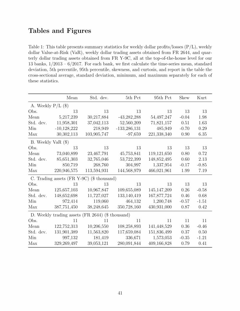
Tables and Figures
Table 1: This table presents summary statistics for weekly dollar profits/losses (P/L), weeklydollar Value-at-Risk (VaR), weekly dollar trading assets obtained from FR 2644, and quar-terly dollar trading assets obtained from FR Y-9C, all at the top-of-the-house level for our13 banks, 1/2013 – 6/2017. For each bank, we first calculate the time-series mean, standarddeviation, 5th percentile, 95th percentile, skewness, and curtosis, and report in the table thecross-sectional average, standard deviation, minimum, and maximum separately for each ofthese statistics.
Mean Std. dev. 5th Pct 95th Pct Skew Kurt
A. Weekly P/L ($)Obs. 13 13 13 13 13 13Mean 5,217,239 30,217,884 -43,282,288 54,497,247 -0.04 1.98Std. dev. 11,958,301 37,042,113 52,560,209 71,821,157 0.51 1.63Min -10,128,222 218,949 -133,286,131 485,949 -0.70 0.29Max 30,302,113 103,905,747 -97,659 221,338,340 0.90 6.35
B. Weekly VaR ($)Obs. 13 13 13 13 13 13Mean 73,040,899 23,467,791 45,753,841 119,121,650 0.80 0.72Std. dev. 85,651,303 32,765,046 53,722,399 148,852,495 0.60 2.13Min 850,719 268,760 304,997 1,337,954 -0.17 -0.85Max 220,946,575 113,594,931 144,568,979 466,021,961 1.99 7.19
C. Trading assets (FR Y-9C) ($ thousand)Obs. 13 13 13 13 13 13Mean 125,657,103 10,967,847 109,655,089 145,147,209 0.26 -0.58Std. dev. 148,652,698 11,727,027 133,140,419 167,877,724 0.46 0.68Min 972,414 119,060 464,132 1,200,748 -0.57 -1.51Max 387,751,450 38,248,645 350,728,160 430,931,000 0.87 0.42
D. Weekly trading assets (FR 2644) ($ thousand)Obs. 11 11 11 11 11 11Mean 122,752,313 10,206,550 108,258,893 141,448,529 0.36 -0.46Std. dev. 131,901,389 11,563,820 117,659,084 151,836,499 0.37 0.50Min 997,132 181,419 336,671 1,573,053 -0.35 -1.21Max 329,269,497 39,053,121 280,091,844 409,166,828 0.79 0.41
41
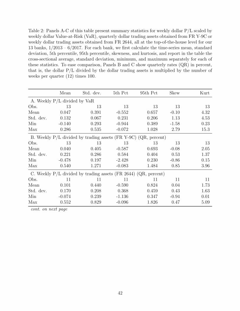
Table 2: Panels A-C of this table present summary statistics for weekly dollar P/L scaled byweekly dollar Value-at-Risk (VaR), quarterly dollar trading assets obtained from FR Y-9C orweekly dollar trading assets obtained from FR 2644, all at the top-of-the-house level for our13 banks, 1/2013 – 6/2017. For each bank, we first calculate the time-series mean, standarddeviation, 5th percentile, 95th percentile, skewness, and kurtosis, and report in the table thecross-sectional average, standard deviation, minimum, and maximum separately for each ofthese statistics. To ease comparison, Panels B and C show quarterly rates (QR) in percent,that is, the dollar P/L divided by the dollar trading assets is multiplied by the number ofweeks per quarter (12) times 100.
Mean Std. dev. 5th Pct 95th Pct Skew Kurt
A. Weekly P/L divided by VaRObs. 13 13 13 13 13 13Mean 0.047 0.391 -0.552 0.657 -0.10 4.32Std. dev. 0.132 0.067 0.231 0.206 1.13 4.53Min -0.140 0.293 -0.944 0.389 -1.58 0.23Max 0.286 0.535 -0.072 1.028 2.79 15.3
B. Weekly P/L divided by trading assets (FR Y-9C) (QR, percent)Obs. 13 13 13 13 13 13Mean 0.040 0.405 -0.587 0.693 -0.08 2.05Std. dev. 0.221 0.286 0.584 0.404 0.53 1.37Min -0.478 0.197 -2.428 0.230 -0.86 0.15Max 0.540 1.271 -0.083 1.484 0.85 3.96
C. Weekly P/L divided by trading assets (FR 2644) (QR, percent)Obs. 11 11 11 11 11 11Mean 0.101 0.440 -0.590 0.824 0.04 1.73Std. dev. 0.170 0.208 0.368 0.459 0.43 1.63Min -0.074 0.239 -1.136 0.347 -0.94 0.01Max 0.552 0.829 -0.096 1.826 0.47 5.09
cont. on next page
42
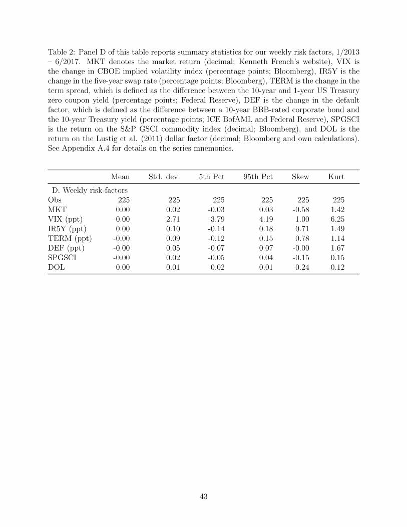
Table 2: Panel D of this table reports summary statistics for our weekly risk factors, 1/2013– 6/2017. MKT denotes the market return (decimal; Kenneth French’s website), VIX isthe change in CBOE implied volatility index (percentage points; Bloomberg), IR5Y is thechange in the five-year swap rate (percentage points; Bloomberg), TERM is the change in theterm spread, which is defined as the difference between the 10-year and 1-year US Treasuryzero coupon yield (percentage points; Federal Reserve), DEF is the change in the defaultfactor, which is defined as the difference between a 10-year BBB-rated corporate bond andthe 10-year Treasury yield (percentage points; ICE BofAML and Federal Reserve), SPGSCIis the return on the S&P GSCI commodity index (decimal; Bloomberg), and DOL is thereturn on the Lustig et al. (2011) dollar factor (decimal; Bloomberg and own calculations).See Appendix A.4 for details on the series mnemonics.
Mean Std. dev. 5th Pct 95th Pct Skew Kurt
D. Weekly risk-factorsObs 225 225 225 225 225 225MKT 0.00 0.02 -0.03 0.03 -0.58 1.42VIX (ppt) -0.00 2.71 -3.79 4.19 1.00 6.25IR5Y (ppt) 0.00 0.10 -0.14 0.18 0.71 1.49TERM (ppt) -0.00 0.09 -0.12 0.15 0.78 1.14DEF (ppt) -0.00 0.05 -0.07 0.07 -0.00 1.67SPGSCI -0.00 0.02 -0.05 0.04 -0.15 0.15DOL -0.00 0.01 -0.02 0.01 -0.24 0.12
43
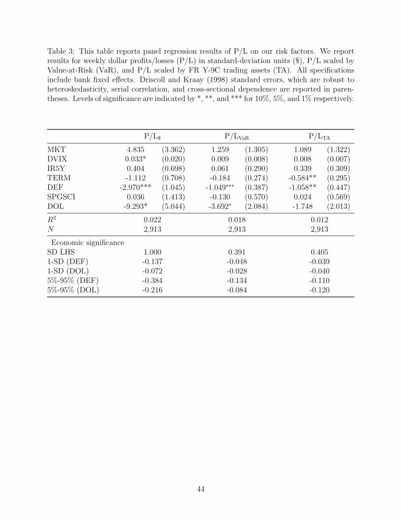
Table 3: This table reports panel regression results of P/L on our risk factors. We reportresults for weekly dollar profits/losses (P/L) in standard-deviation units ($), P/L scaled byValue-at-Risk (VaR), and P/L scaled by FR Y-9C trading assets (TA). All specificationsinclude bank fixed effects. Driscoll and Kraay (1998) standard errors, which are robust toheteroskedasticity, serial correlation, and cross-sectional dependence are reported in paren-theses. Levels of significance are indicated by *, **, and *** for 10%, 5%, and 1% respectively.
P/L$ P/LVaR P/LTA
MKT 4.835 (3.362) 1.259 (1.305) 1.089 (1.322)DVIX 0.033* (0.020) 0.009 (0.008) 0.008 (0.007)IR5Y 0.404 (0.698) 0.061 (0.290) 0.339 (0.309)TERM -1.112 (0.708) -0.184 (0.274) -0.584** (0.295)DEF -2.970*** (1.045) -1.049∗∗∗ (0.387) -1.058** (0.447)SPGSCI 0.036 (1.413) -0.130 (0.570) 0.024 (0.569)DOL -9.293* (5.044) -3.692∗ (2.084) -1.748 (2.013)
R2 0.022 0.018 0.012N 2,913 2,913 2,913
Economic significanceSD LHS 1.000 0.391 0.4051-SD (DEF) -0.137 -0.048 -0.0391-SD (DOL) -0.072 -0.028 -0.0405%-95% (DEF) -0.384 -0.134 -0.1105%-95% (DOL) -0.216 -0.084 -0.120
44
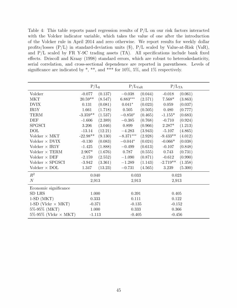
Table 4: This table reports panel regression results of P/L on our risk factors interactedwith the Volcker indicator variable, which takes the value of one after the introductionof the Volcker rule in April 2014 and zero otherwise. We report results for weekly dollarprofits/losses (P/L) in standard-deviation units ($), P/L scaled by Value-at-Risk (VaR),and P/L scaled by FR Y-9C trading assets (TA). All specifications include bank fixedeffects. Driscoll and Kraay (1998) standard errors, which are robust to heteroskedasticity,serial correlation, and cross-sectional dependence are reported in parentheses. Levels ofsignificance are indicated by *, **, and *** for 10%, 5%, and 1% respectively.
P/L$ P/LVaR P/LTA
Volcker -0.077 (0.137) −0.038 (0.044) -0.018 (0.061)MKT 20.59** (8.547) 6.883∗∗∗ (2.571) 7.568* (3.863)DVIX 0.131 (0.081) 0.041∗ (0.023) 0.059 (0.037)IR5Y 1.661 (1.718) 0.505 (0.505) 0.480 (0.777)TERM -3.359** (1.537) −0.850∗ (0.465) -1.155* (0.683)DEF -1.606 (2.389) −0.385 (0.768) -0.710 (0.924)SPGSCI 3.206 (3.046) 0.899 (0.966) 2.287* (1.213)DOL -13.14 (12.21) −4.283 (3.943) -5.107 (4.865)Volcker × MKT -22.98** (9.130) −8.371∗∗∗ (2.928) -9.433** (4.012)Volcker × DVIX -0.130 (0.083) −0.044∗ (0.024) -0.066* (0.038)Volcker × IR5Y -1.425 (1.888) −0.499 (0.613) -0.107 (0.848)Volcker × TERM 2.907* (1.676) 0.787 (0.555) 0.743 (0.731)Volcker × DEF -2.159 (2.552) −1.090 (0.871) -0.612 (0.990)Volcker × SPGSCI -3.942 (3.361) −1.289 (1.143) -2.719** (1.358)Volcker × DOL 1.347 (13.23) −0.731 (4.565) 3.239 (5.300)
R2 0.040 0.033 0.023N 2,913 2,913 2,913
Economic significanceSD LHS 1.000 0.391 0.4051-SD (MKT) 0.333 0.111 0.1221-SD (Vlckr × MKT) -0.371 -0.135 -0.1525%-95% (MKT) 1.000 0.333 0.3665%-95% (Vlckr × MKT) -1.113 -0.405 -0.456
45
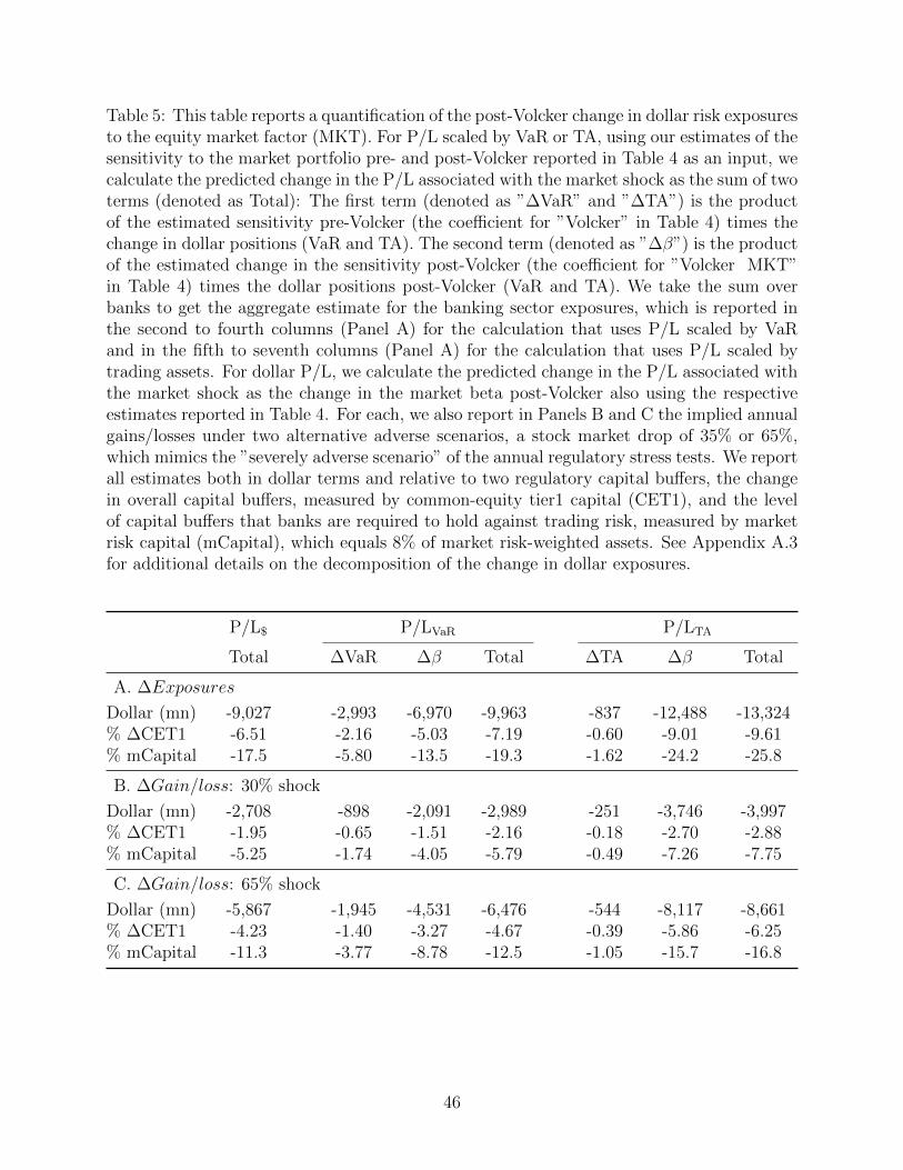
Table 5: This table reports a quantification of the post-Volcker change in dollar risk exposuresto the equity market factor (MKT). For P/L scaled by VaR or TA, using our estimates of thesensitivity to the market portfolio pre- and post-Volcker reported in Table 4 as an input, wecalculate the predicted change in the P/L associated with the market shock as the sum of twoterms (denoted as Total): The first term (denoted as ”∆VaR” and ”∆TA”) is the productof the estimated sensitivity pre-Volcker (the coefficient for ”Volcker” in Table 4) times thechange in dollar positions (VaR and TA). The second term (denoted as ”∆β”) is the productof the estimated change in the sensitivity post-Volcker (the coefficient for ”Volcker MKT”in Table 4) times the dollar positions post-Volcker (VaR and TA). We take the sum overbanks to get the aggregate estimate for the banking sector exposures, which is reported inthe second to fourth columns (Panel A) for the calculation that uses P/L scaled by VaRand in the fifth to seventh columns (Panel A) for the calculation that uses P/L scaled bytrading assets. For dollar P/L, we calculate the predicted change in the P/L associated withthe market shock as the change in the market beta post-Volcker also using the respectiveestimates reported in Table 4. For each, we also report in Panels B and C the implied annualgains/losses under two alternative adverse scenarios, a stock market drop of 35% or 65%,which mimics the ”severely adverse scenario” of the annual regulatory stress tests. We reportall estimates both in dollar terms and relative to two regulatory capital buffers, the changein overall capital buffers, measured by common-equity tier1 capital (CET1), and the levelof capital buffers that banks are required to hold against trading risk, measured by marketrisk capital (mCapital), which equals 8% of market risk-weighted assets. See Appendix A.3for additional details on the decomposition of the change in dollar exposures.
P/L$ P/LVaR P/LTA
Total ∆VaR ∆β Total ∆TA ∆β Total
A. ∆Exposures
Dollar (mn) -9,027 -2,993 -6,970 -9,963 -837 -12,488 -13,324% ∆CET1 -6.51 -2.16 -5.03 -7.19 -0.60 -9.01 -9.61% mCapital -17.5 -5.80 -13.5 -19.3 -1.62 -24.2 -25.8
B. ∆Gain/loss: 30% shock
Dollar (mn) -2,708 -898 -2,091 -2,989 -251 -3,746 -3,997% ∆CET1 -1.95 -0.65 -1.51 -2.16 -0.18 -2.70 -2.88% mCapital -5.25 -1.74 -4.05 -5.79 -0.49 -7.26 -7.75
C. ∆Gain/loss: 65% shock
Dollar (mn) -5,867 -1,945 -4,531 -6,476 -544 -8,117 -8,661% ∆CET1 -4.23 -1.40 -3.27 -4.67 -0.39 -5.86 -6.25% mCapital -11.3 -3.77 -8.78 -12.5 -1.05 -15.7 -16.8
46
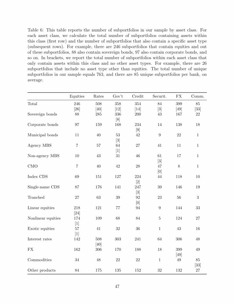
Table 6: This table reports the number of subportfolios in our sample by asset class. Foreach asset class, we calculate the total number of subportfolios containing assets withinthis class (first row) and the number of subportfolios that also contain a specific asset type(subsequent rows). For example, there are 246 subportfolios that contain equities and outof these subportfolios, 88 also contain sovereign bonds, 97 also contain corporate bonds, andso on. In brackets, we report the total number of subportfolios within each asset class thatonly contain assets within this class and no other asset types. For example, there are 26subportfolios that include no asset type other than equities. The total number of uniquesubportfolios in our sample equals 763, and there are 85 unique subportfolios per bank, onaverage.
Equities Rates Gov’t Credit Securit. FX Comm.
Total 246 508 358 354 84 399 85[26] [40] [12] [14] [3] [49] [33]
Sovereign bonds 88 285 336 200 43 167 22[8]
Corporate bonds 97 159 168 234 14 138 18[9]
Municipal bonds 11 40 53 42 9 22 1[3]
Agency MBS 7 57 64 27 41 11 1[1]
Non-agency MBS 10 43 31 46 61 17 1[3]
CMO 7 40 42 28 47 8 1[0]
Index CDS 69 151 127 224 44 118 10[2]
Single-name CDS 87 176 141 247 39 146 19[3]
Tranched 27 63 39 92 23 56 3[0]
Linear equities 218 121 77 94 9 144 33[24]
Nonlinear equities 174 109 68 84 5 124 27[1]
Exotic equities 57 41 32 36 1 43 16[1]
Interest rates 142 508 303 241 64 306 48[40]
FX 162 306 170 188 18 399 49[49]
Commodities 34 48 22 22 1 49 85[33]
Other products 84 175 135 152 32 132 27
47
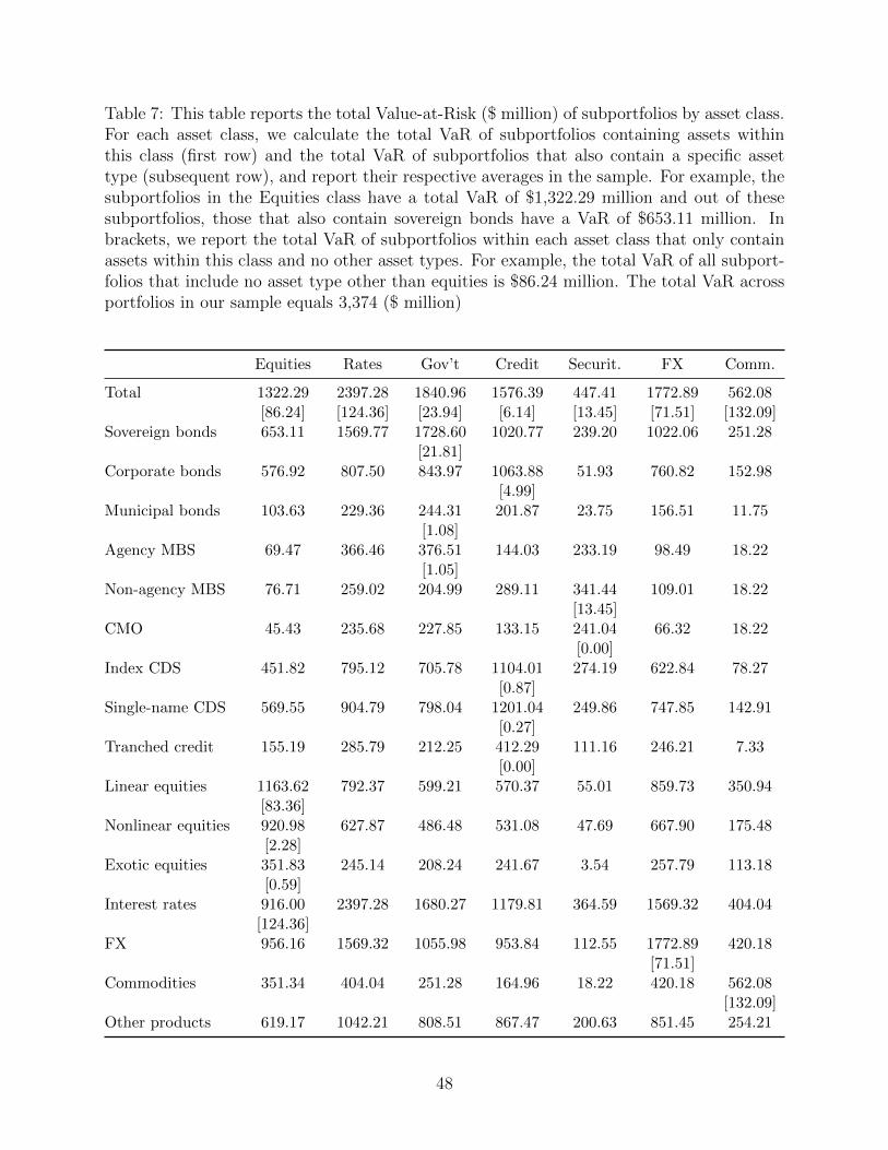
Table 7: This table reports the total Value-at-Risk ($ million) of subportfolios by asset class.For each asset class, we calculate the total VaR of subportfolios containing assets withinthis class (first row) and the total VaR of subportfolios that also contain a specific assettype (subsequent row), and report their respective averages in the sample. For example, thesubportfolios in the Equities class have a total VaR of $1,322.29 million and out of thesesubportfolios, those that also contain sovereign bonds have a VaR of $653.11 million. Inbrackets, we report the total VaR of subportfolios within each asset class that only containassets within this class and no other asset types. For example, the total VaR of all subport-folios that include no asset type other than equities is $86.24 million. The total VaR acrossportfolios in our sample equals 3,374 ($ million)
Equities Rates Gov’t Credit Securit. FX Comm.
Total 1322.29 2397.28 1840.96 1576.39 447.41 1772.89 562.08[86.24] [124.36] [23.94] [6.14] [13.45] [71.51] [132.09]
Sovereign bonds 653.11 1569.77 1728.60 1020.77 239.20 1022.06 251.28[21.81]
Corporate bonds 576.92 807.50 843.97 1063.88 51.93 760.82 152.98[4.99]
Municipal bonds 103.63 229.36 244.31 201.87 23.75 156.51 11.75[1.08]
Agency MBS 69.47 366.46 376.51 144.03 233.19 98.49 18.22[1.05]
Non-agency MBS 76.71 259.02 204.99 289.11 341.44 109.01 18.22[13.45]
CMO 45.43 235.68 227.85 133.15 241.04 66.32 18.22[0.00]
Index CDS 451.82 795.12 705.78 1104.01 274.19 622.84 78.27[0.87]
Single-name CDS 569.55 904.79 798.04 1201.04 249.86 747.85 142.91[0.27]
Tranched credit 155.19 285.79 212.25 412.29 111.16 246.21 7.33[0.00]
Linear equities 1163.62 792.37 599.21 570.37 55.01 859.73 350.94[83.36]
Nonlinear equities 920.98 627.87 486.48 531.08 47.69 667.90 175.48[2.28]
Exotic equities 351.83 245.14 208.24 241.67 3.54 257.79 113.18[0.59]
Interest rates 916.00 2397.28 1680.27 1179.81 364.59 1569.32 404.04[124.36]
FX 956.16 1569.32 1055.98 953.84 112.55 1772.89 420.18[71.51]
Commodities 351.34 404.04 251.28 164.96 18.22 420.18 562.08[132.09]
Other products 619.17 1042.21 808.51 867.47 200.63 851.45 254.21
48

Table 8: This table reports panel regression results for the P/L with alternative normal-izations at the subportfolio level. We report results for weekly dollar profits/losses (P/L)in standard-deviation units ($), P/L scaled by Value-at-Risk (VaR), and P/L scaled by FRY-9C trading assets (TA). For each asset class, we regress the normalized subportfolio P/Lon our risk factors interacted with the Volcker indicator variable, which takes the value ofone after the introduction of the Volcker rule in April 2014 and zero otherwise. For read-ability, we report the main estimates for the MKT factor and omit the estimates for theother factors, which are reported in Appendix Table A11. All specifications include bankfixed effects. Driscoll and Kraay (1998) standard errors, which are robust to heteroskedas-ticity, serial correlation, and cross-sectional dependence are reported in parentheses. Levelsof significance are indicated by *, **, and *** for 10%, 5%, and 1% respectively.
Equities Rates Gov’t Credit Securit. FX Comm.
A. P/L$
Volcker -0.107*** -0.052 -0.018 -0.093* -0.118 -0.100*** -0.054(0.035) (0.037) (0.061) (0.054) (0.082) (0.025) (0.048)
MKT 5.326*** 3.105* 5.971** 3.833* -0.654 3.092** -6.429***(1.509) (1.599) (2.342) (2.063) (3.025) (1.534) (2.470)
Volcker × MKT -4.063** -2.367 -5.277** -3.945* 0.124 -2.431 5.840**(1.804) (1.765) (2.512) (2.278) (3.146) (1.755) (2.790)
R2 0.004 0.001 0.002 0.003 0.002 0.002 0.002N 39,747 74,905 54,951 51,262 11,815 59,888 12,152
B. P/LVaR
Volcker -0.025 -0.020 0.003 -0.013 -0.039 -0.044* -0.029(0.023) (0.026) (0.019) (0.020) (0.120) (0.026) (0.023)
MKT 4.474*** 6.557** 3.705** 2.442* 23.79 7.010** -0.373(1.512) (3.101) (1.469) (1.452) (15.25) (3.476) (1.302)
Volcker × MKT -4.128** -6.998** -4.231*** -2.807* -25.66* -6.981* 2.461(1.705) (3.187) (1.612) (1.614) (15.54) (3.598) (1.957)
R2 0.002 0.001 0.002 0.001 0.002 0.001 0.004N 39,747 74,905 55,000 51,311 11,815 59,888 12,152
C. P/LTA
Volcker -0.133*** -0.095** -0.013 -0.204*** -0.150* -0.151*** -0.200**(0.030) (0.037) (0.085) (0.063) (0.090) (0.042) (0.085)
MKT 5.414*** 1.921 7.359* 5.911** 0.801 2.460 -5.437(2.035) (1.774) (4.367) (2.526) (2.613) (2.022) (3.814)
Volcker × MKT -6.493** -2.454 -8.071* -5.324* -0.702 -2.295 3.980(2.567) (2.070) (4.534) (2.767) (3.082) (2.306) (4.074)
R2 0.015 0.001 0.001 0.008 0.004 0.001 0.006N 5,218 16,575 14,021 8,687 1,571 10,069 2,447
49
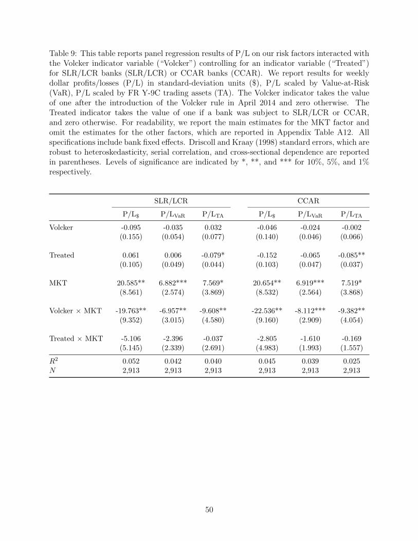
Table 9: This table reports panel regression results of P/L on our risk factors interacted withthe Volcker indicator variable (“Volcker”) controlling for an indicator variable (“Treated”)for SLR/LCR banks (SLR/LCR) or CCAR banks (CCAR). We report results for weeklydollar profits/losses (P/L) in standard-deviation units ($), P/L scaled by Value-at-Risk(VaR), P/L scaled by FR Y-9C trading assets (TA). The Volcker indicator takes the valueof one after the introduction of the Volcker rule in April 2014 and zero otherwise. TheTreated indicator takes the value of one if a bank was subject to SLR/LCR or CCAR,and zero otherwise. For readability, we report the main estimates for the MKT factor andomit the estimates for the other factors, which are reported in Appendix Table A12. Allspecifications include bank fixed effects. Driscoll and Kraay (1998) standard errors, which arerobust to heteroskedasticity, serial correlation, and cross-sectional dependence are reportedin parentheses. Levels of significance are indicated by *, **, and *** for 10%, 5%, and 1%respectively.
SLR/LCR CCAR
P/L$ P/LVaR P/LTA P/L$ P/LVaR P/LTA
Volcker -0.095 -0.035 0.032 -0.046 -0.024 -0.002(0.155) (0.054) (0.077) (0.140) (0.046) (0.066)
Treated 0.061 0.006 -0.079* -0.152 -0.065 -0.085**(0.105) (0.049) (0.044) (0.103) (0.047) (0.037)
MKT 20.585** 6.882*** 7.569* 20.654** 6.919*** 7.519*(8.561) (2.574) (3.869) (8.532) (2.564) (3.868)
Volcker × MKT -19.763** -6.957** -9.608** -22.536** -8.112*** -9.382**(9.352) (3.015) (4.580) (9.160) (2.909) (4.054)
Treated × MKT -5.106 -2.396 -0.037 -2.805 -1.610 -0.169(5.145) (2.339) (2.691) (4.983) (1.993) (1.557)
R2 0.052 0.042 0.040 0.045 0.039 0.025N 2,913 2,913 2,913 2,913 2,913 2,913
50
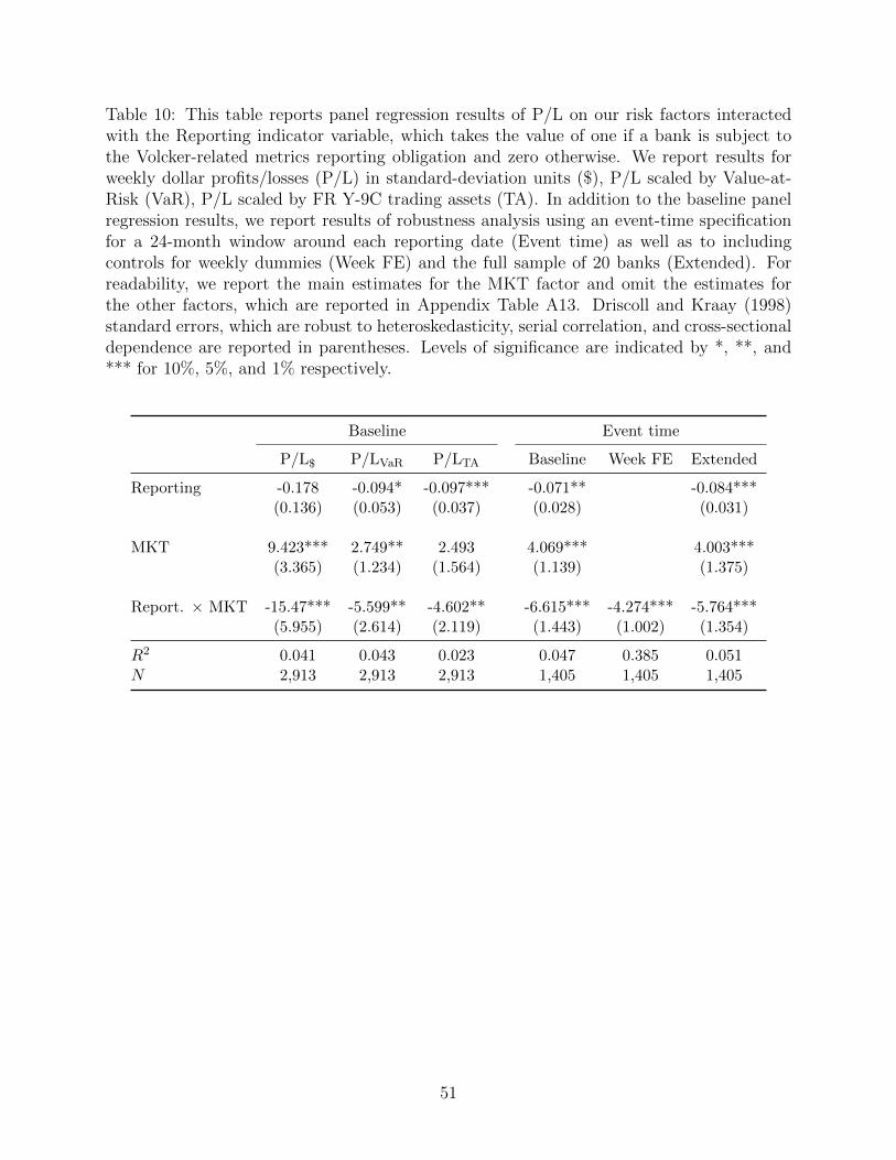
Table 10: This table reports panel regression results of P/L on our risk factors interactedwith the Reporting indicator variable, which takes the value of one if a bank is subject tothe Volcker-related metrics reporting obligation and zero otherwise. We report results forweekly dollar profits/losses (P/L) in standard-deviation units ($), P/L scaled by Value-at-Risk (VaR), P/L scaled by FR Y-9C trading assets (TA). In addition to the baseline panelregression results, we report results of robustness analysis using an event-time specificationfor a 24-month window around each reporting date (Event time) as well as to includingcontrols for weekly dummies (Week FE) and the full sample of 20 banks (Extended). Forreadability, we report the main estimates for the MKT factor and omit the estimates forthe other factors, which are reported in Appendix Table A13. Driscoll and Kraay (1998)standard errors, which are robust to heteroskedasticity, serial correlation, and cross-sectionaldependence are reported in parentheses. Levels of significance are indicated by *, **, and*** for 10%, 5%, and 1% respectively.
Baseline Event time
P/L$ P/LVaR P/LTA Baseline Week FE Extended
Reporting -0.178 -0.094* -0.097*** -0.071** -0.084***(0.136) (0.053) (0.037) (0.028) (0.031)
MKT 9.423*** 2.749** 2.493 4.069*** 4.003***(3.365) (1.234) (1.564) (1.139) (1.375)
Report. × MKT -15.47*** -5.599** -4.602** -6.615*** -4.274*** -5.764***(5.955) (2.614) (2.119) (1.443) (1.002) (1.354)
R2 0.041 0.043 0.023 0.047 0.385 0.051N 2,913 2,913 2,913 1,405 1,405 1,405
51
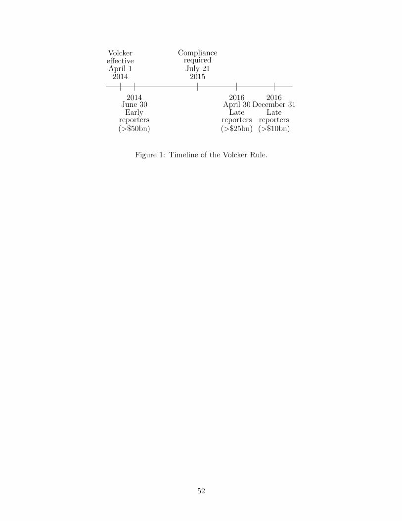
VolckereffectiveApril 12014
CompliancerequiredJuly 21
2015
2014June 30Early
reporters(>$50bn)
2016April 30
Latereporters(>$25bn)
2016December 31
Latereporters(>$10bn)
Figure 1: Timeline of the Volcker Rule.
52
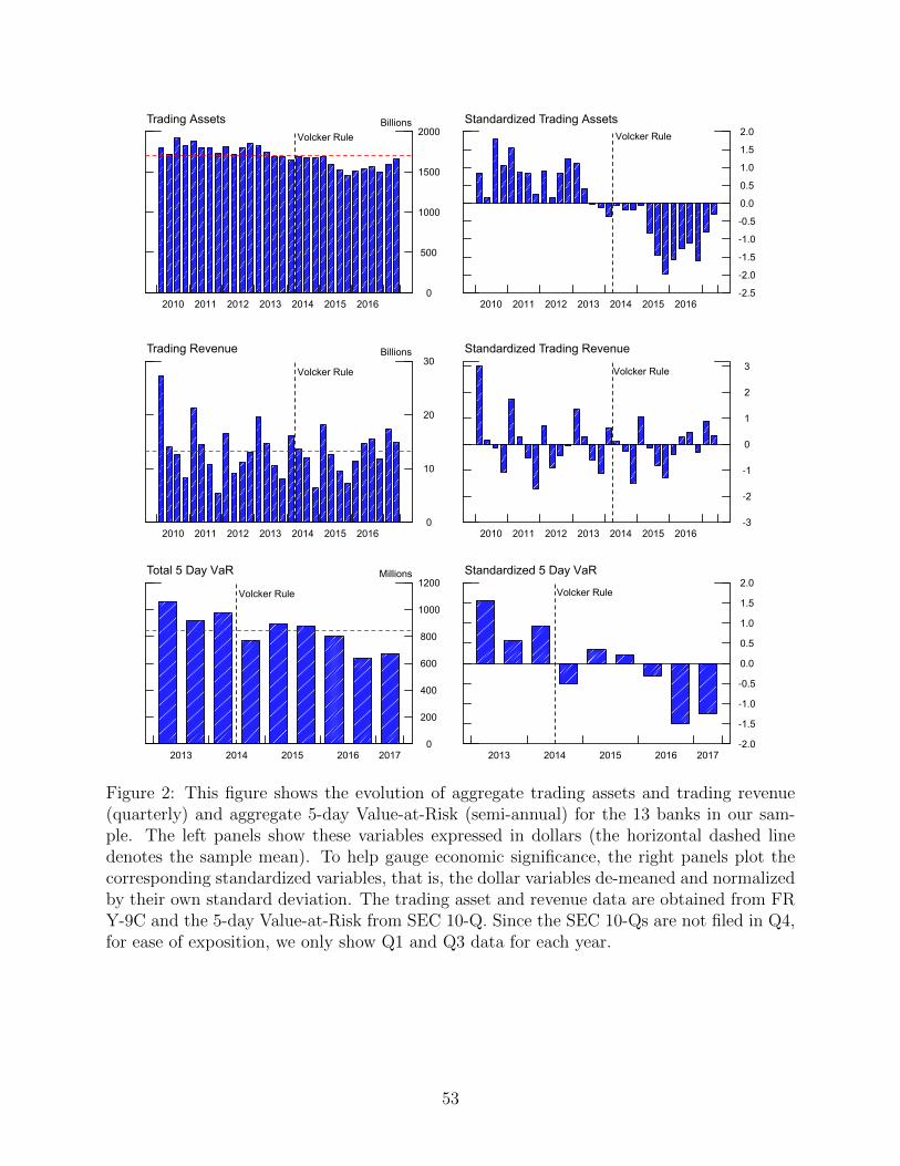
0
500
1000
1500
2000
2010 2011 2012 2013 2014 2015 2016
BillionsTrading AssetsVolcker Rule
-0.5
-1.0
-1.5
-2.0
-2.5
0.0
0.5
1.0
1.5
2.0
2010 2011 2012 2013 2014 2015 2016
Standardized Trading AssetsVolcker Rule
0
10
20
30
2010 2011 2012 2013 2014 2015 2016
BillionsTrading Revenue
Volcker Rule
-1
-2
-3
0
1
2
3
2010 2011 2012 2013 2014 2015 2016
Standardized Trading Revenue
Volcker Rule
0
200
400
600
800
1000
1200
2013 2014 2015 2016 2017
MillionsTotal 5 Day VaR
Volcker Rule
-0.5
-1.0
-1.5
-2.0
0.0
0.5
1.0
1.5
2.0
2013 2014 2015 2016 2017
Standardized 5 Day VaR
Volcker Rule
Figure 2: This figure shows the evolution of aggregate trading assets and trading revenue(quarterly) and aggregate 5-day Value-at-Risk (semi-annual) for the 13 banks in our sam-ple. The left panels show these variables expressed in dollars (the horizontal dashed linedenotes the sample mean). To help gauge economic significance, the right panels plot thecorresponding standardized variables, that is, the dollar variables de-meaned and normalizedby their own standard deviation. The trading asset and revenue data are obtained from FRY-9C and the 5-day Value-at-Risk from SEC 10-Q. Since the SEC 10-Qs are not filed in Q4,for ease of exposition, we only show Q1 and Q3 data for each year.
53
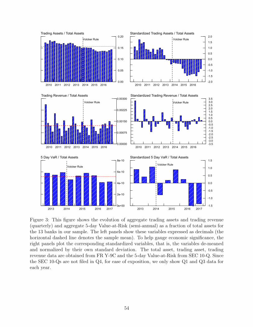
0.00
0.05
0.10
0.15
0.20
2010 2011 2012 2013 2014 2015 2016
Trading Assets / Total Assets
Volcker Rule
-0.5
-1.0
-1.5
-2.0
0.0
0.5
1.0
1.5
2.0
2010 2011 2012 2013 2014 2015 2016
Standardized Trading Assets / Total Assets
Volcker Rule
0.00000
0.00075
0.00150
0.00225
0.00300
2010 2011 2012 2013 2014 2015 2016
Trading Revenue / Total Assets
Volcker Rule
-0.5-1.0-1.5-2.0-2.5-3.0-3.5
0.00.51.01.52.02.53.03.5
2010 2011 2012 2013 2014 2015 2016
Standardized Trading Revenue / Total Assets
Volcker Rule
0e+00
2e-10
4e-10
6e-10
8e-10
2013 2014 2015 2016 2017
5 Day VaR / Total Assets
Volcker Rule
-0.5
-1.0
-1.5
0.0
0.5
1.0
1.5
2013 2014 2015 2016 2017
Standardized 5 Day VaR / Total Assets
Volcker Rule
Figure 3: This figure shows the evolution of aggregate trading assets and trading revenue(quarterly) and aggregate 5-day Value-at-Risk (semi-annual) as a fraction of total assets forthe 13 banks in our sample. The left panels show these variables expressed as decimals (thehorizontal dashed line denotes the sample mean). To help gauge economic significance, theright panels plot the corresponding standardized variables, that is, the variables de-meanedand normalized by their own standard deviation. The total asset, trading asset, tradingrevenue data are obtained from FR Y-9C and the 5-day Value-at-Risk from SEC 10-Q. Sincethe SEC 10-Qs are not filed in Q4, for ease of exposition, we only show Q1 and Q3 data foreach year.
54
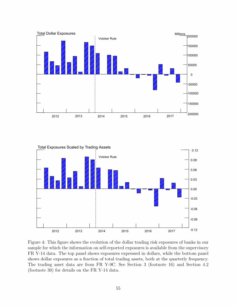
-100000
-150000
-200000
-50000
0
50000
100000
150000
200000
2012 2013 2014 2015 2016 2017
MillionsTotal Dollar ExposuresVolcker Rule
-0.03
-0.06
-0.09
-0.12
0.00
0.03
0.06
0.09
0.12
2012 2013 2014 2015 2016 2017
Total Exposures Scaled by Trading Assets
Volcker Rule
Figure 4: This figure shows the evolution of the dollar trading risk exposures of banks in oursample for which the information on self-reported exposures is available from the supervisoryFR Y-14 data. The top panel shows exposures expressed in dollars, while the bottom panelshows dollar exposures as a fraction of total trading assets, both at the quarterly frequency.The trading asset data are from FR Y-9C. See Section 3 (footnote 16) and Section 4.2(footnote 30) for details on the FR Y-14 data.
55
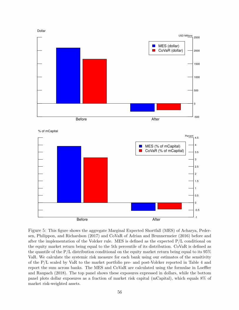
-500
0
500
1000
1500
2000
2500
Before After
USD Millions
Dollar
MES (dollar)CoVaR (dollar)
-1
-0.5
0
0.5
1
1.5
2
2.5
3
3.5
4
4.5
Before After
Percent
% of mCapital
MES (% of mCapital)CoVaR (% of mCapital)
-500
0
500
1000
1500
2000
2500
Before After
USD Millions
Dollar
MES (dollar)CoVaR (dollar)
-1
-0.5
0
0.5
1
1.5
2
2.5
3
3.5
4
4.5
Before After
Percent
% of mCapital
MES (% of mCapital)CoVaR (% of mCapital)
Figure 5: This figure shows the aggregate Marginal Expected Shortfall (MES) of Acharya, Peder-sen, Philippon, and Richardson (2017) and CoVaR of Adrian and Brunnermeier (2016) before andafter the implementation of the Volcker rule. MES is defined as the expected P/L conditional onthe equity market return being equal to the 5th percentile of its distribution. CoVaR is defined asthe quantile of the P/L distribution conditional on the equity market return being equal to its 95%VaR. We calculate the systemic risk measure for each bank using our estimates of the sensitivityof the P/L scaled by VaR to the market portfolio pre- and post-Volcker reported in Table 4 andreport the sum across banks. The MES and CoVaR are calculated using the formulae in Loefflerand Raupach (2018). The top panel shows these exposures expressed in dollars, while the bottompanel plots dollar exposures as a fraction of market risk capital (mCapital), which equals 8% ofmarket risk-weighted assets.
56
Internet Appendix for
“Banks as Regulated Traders”
Antonio Falato Diana Iercosan Filip Zikes
July 29, 2021
A.1 Volcker rule, market making exemption, and risk
exposures: Additional details on institutional back-
ground
The Volcker rule generally prohibits any insured depositary institution, or a company that
controls an insured depositary institutions, from engaging in proprietary trading and invest-
ing in certain investment funds, such as private equity and hedge funds (Federal Register,
2014, §3 and 10, pp. 5781–5796). The rule exempts certain activities from the propri-
etary trading prohibition. The permitted activities include underwriting, market making,
risk-mitigating hedging, and some other activities such as proprietary trading in govern-
ment securities, trading on behalf of customers, trading by insurance companies and certain
foreign banking entities (Federal Register, 2014, §4-6, pp. 5783–5786). Below, we discuss
the elements of the rule that are relevant for our analysis of banks trading book exposures,
namely the market making exemptions, the compliance requirements and metrics reporting,
and the nature of financial exposures the rule intends to curb.
The market making exemption allows covered banking entities to engage in market-
making related activities that are genuinely client-facing and designed not to exceed the
reasonable expected near-term demands of clients, customers, and counterparties (Federal
1
Register, 2014, §4(b), pp. 5783–5784). Specifically, the rule requires banking entities in-
voking the market making exemptions to routinely stand ready to buy or sell one or more
types of financial instruments for its own account in commercially reasonable amounts and
throughout market cycles, reflecting the market liquidity and maturity of the instruments
traded (Federal Register, 2014, §4(b)(2)(i)). The banking entity has to ensure that the
amount, types, and risk of the financial instruments in the trading desks market making
inventory do not exceed, on an ongoing basis, the reasonably expected near-term demands
of clients, customers, and counterparties, based on the market liquidity and maturity and
demonstrable analysis of historical and projected customer demand (Federal Register, 2014,
§4(b)(2)(ii)). The banking entity has to establish and comply with written policies and pro-
cedures that include describing the financial instruments in which it is trading, actions taken
to manage the risks associated with its financial exposures, limits on its market-making in-
ventory, financial exposures, allowable risks, and hedging activities, procedures for dealing
with breaches of these limits, and appropriate internal controls and monitoring of compliance
at the trading desk level (Federal Register, 2014, §4(b)(2)(iii-iv)).
Banking entities that engage in trading or investment activities covered by the rule have
to develop a reasonably designed compliance program that allows for continued monitoring of
compliance with the rule (Federal Registers, 2014, §20-21, pp. 5796–5797). This compliance
program includes reporting and record keeping requirements designed to allow regulators to
identify and detect prohibited proprietary trading and high-risk trading strategies (Federal
Register, 2014, Appendix A, pp. 5797–5800). Specifically, banking entities subject to the
reporting requirement, discussed in the paper, have to periodically furnish to the relevant
Agency a set of quantitative measurements, including risk and positions limits and usage; risk
factor sensitivities; Value at Risk and stressed Value at Risk; comprehensive profit and loss
attribution; inventory turnover; inventory aging; and customer-facing trade ratio (Federal
Register, 2014, Appendix A(III)(a), p. 5798). These metrics have to be reported for each
trading day (Federal Register, 2014, Appendix A(III)(b), p. 5798).
Although the final implementation of the rule does not impose specific limits for individual
metrics, it makes it clear that monitoring of compliance includes making sure the firms set
and adhere to appropriate self-imposed limits in line with their market making and hedging
2

activity. As such, the rule does not require that overall risk, as measured by volatility
or VaR, necessarily decrease. Rather, the nature of risk that firms are permitted to take
on under the rule is expected to be consistent with prudent market making, underwriting,
or hedging, profits or losses of which generally exhibit little correlation with aggregate risk
factors. Importantly, financial exposure is understood to be exposure to all significant market
factors driving the financial instruments in which a firm act as a market maker or that it uses
for risk management purposes (Federal Register, 2014, p. 5594). The idea is that risk factor
sensitivities are more suitable for detecting prohibited activities than simple risk measures,
because speculative trading is typically characterized by taking directional positions aimed
at profiting from price changes (Federal Register, 2014, p. 5618), that is, features that
volatility or VaR cannot generally detect. The trading activities that are exempt from the
proprietary trading prohibition, such as market making, while still being able to generate
considerable volatility and VaR, nonetheless typically exhibit less directional exposures to
common risk factors, as these strategies typically hedge the associate market risk and derive
profit from bid-ask spreads, commissions, and other fees. Although the final rule does not
require these fees to be the only source of revenue from permitted market making activity,
the Agencies make it clear that evaluating the source of profits and losses will constitute an
important part of determining whether a trading activity constitutes prohibited proprietary
trading (Federal Register, 2014, p. 5623).
A.2 Scaling by VaR: Additional details on measure-
ment
Consider a stylized location-scale model, where the profits (P/L) are given by
P/Lt = µt−1 + σt−1Zt,
where µt−1 is the conditional mean and σt−1 is the conditional volatility of P/Lt at time t−1
and Zt is a sequence of independently and identically distributed innovations with zero mean
and unit variance. Because we are modelling the clean P/L at weekly frequency, which has a
3
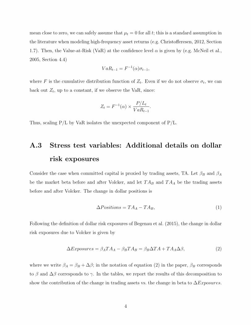
mean close to zero, we can safely assume that µt = 0 for all t; this is a standard assumption in
the literature when modeling high-frequency asset returns (e.g. Christofferesen, 2012, Section
1.7). Then, the Value-at-Risk (VaR) at the confidence level α is given by (e.g. McNeil et al.,
2005, Section 4.4)
V aRt−1 = F−1(α)σt−1,
where F is the cumulative distribution function of Zt. Even if we do not observe σt, we can
back out Zt, up to a constant, if we observe the VaR, since:
Zt = F−1(α)× P/LtV aRt−1
.
Thus, scaling P/L by VaR isolates the unexpected component of P/L.
A.3 Stress test variables: Additional details on dollar
risk exposures
Consider the case when committed capital is proxied by trading assets, TA. Let βB and βA
be the market beta before and after Volcker, and let TAB and TAA be the trading assets
before and after Volcker. The change in dollar positions is
∆Positions = TAA − TAB, (1)
Following the definition of dollar risk exposures of Begenau et al. (2015), the change in dollar
risk exposures due to Volcker is given by
∆Exposures = βATAA − βBTAB = βB∆TA+ TAA∆β, (2)
where we write βA = βB + ∆β; in the notation of equation (2) in the paper, βB corresponds
to β and ∆β corresponds to γ. In the tables, we report the results of this decomposition to
show the contribution of the change in trading assets vs. the change in beta to ∆Exposures.
4
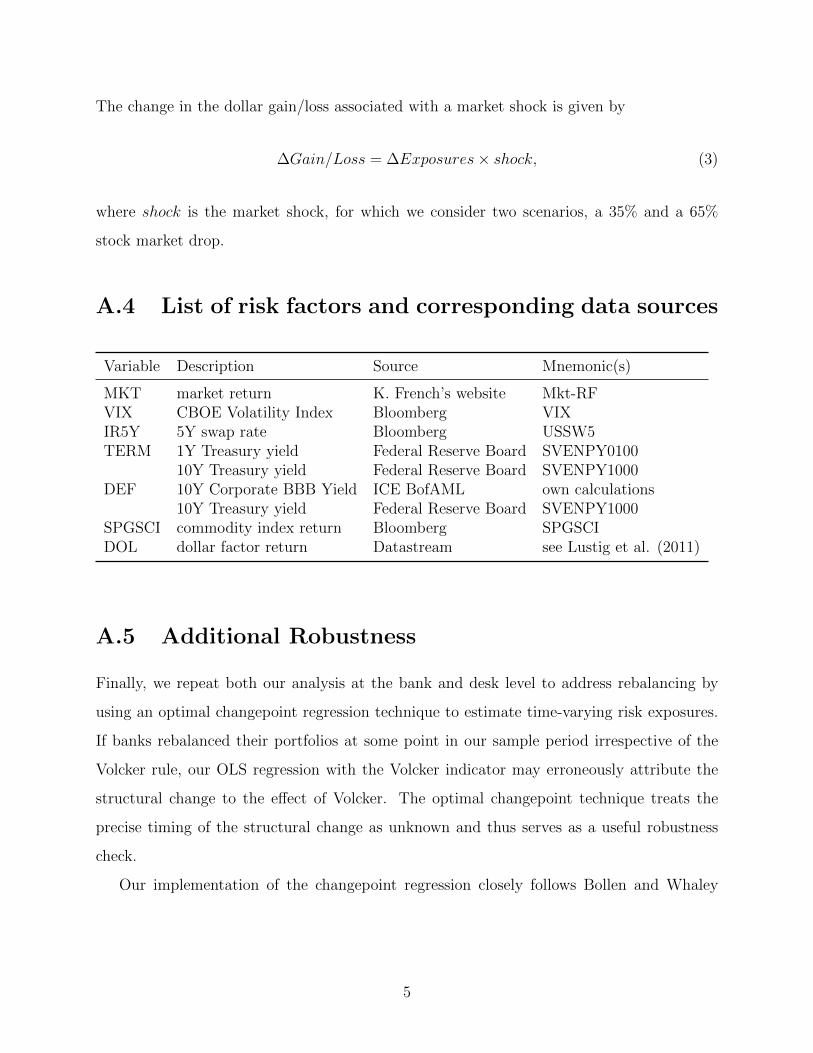
The change in the dollar gain/loss associated with a market shock is given by
∆Gain/Loss = ∆Exposures× shock, (3)
where shock is the market shock, for which we consider two scenarios, a 35% and a 65%
stock market drop.
A.4 List of risk factors and corresponding data sources
Variable Description Source Mnemonic(s)
MKT market return K. French’s website Mkt-RFVIX CBOE Volatility Index Bloomberg VIXIR5Y 5Y swap rate Bloomberg USSW5TERM 1Y Treasury yield Federal Reserve Board SVENPY0100
10Y Treasury yield Federal Reserve Board SVENPY1000DEF 10Y Corporate BBB Yield ICE BofAML own calculations
10Y Treasury yield Federal Reserve Board SVENPY1000SPGSCI commodity index return Bloomberg SPGSCIDOL dollar factor return Datastream see Lustig et al. (2011)
A.5 Additional Robustness
Finally, we repeat both our analysis at the bank and desk level to address rebalancing by
using an optimal changepoint regression technique to estimate time-varying risk exposures.
If banks rebalanced their portfolios at some point in our sample period irrespective of the
Volcker rule, our OLS regression with the Volcker indicator may erroneously attribute the
structural change to the effect of Volcker. The optimal changepoint technique treats the
precise timing of the structural change as unknown and thus serves as a useful robustness
check.
Our implementation of the changepoint regression closely follows Bollen and Whaley
5

(2009). In particular, for each portfolio and each π, 0 < π < 1, we run the regressions
rit = α0i + βi0RFt + εit, t = 1, ..., πT,
rit = α0i + α1i + (β0i + β1i)RFt + εit, t = πT + 1, ..., T,
and calculate the F-statistic, F (π), for the null hypothesis that α1i = β1i = 0. The test for
a structural break at an unknown date is then based on the average F-statistic,∑
π F (π).
Following Bollen and Whaley (2009), we approximate the critical values for this statistic by
bootstrap and estimate the date of the structural break by minimizing (over π) the sum of
squared residuals in the model above. The additional benefit of this approach is that we
can implement a statistical test for structural breaks in banks’ and desks’ equity market
risk exposures similar to Bollen and Whaley (2009), who show that the optimal changepoint
method is superior to a stochastic parameter model in detecting time-varying exposures.
The results are reported in Figure A4, which plots the cumulative frequencies of banks
(right axis) and trading desks (left axis) that experience a significant structural break in
their equity market beta in any given quarter over our sample period. In line with our OLS
results, about half (40%) of the banks (desks) experienced a break in equity risk exposure
in the quarters after the rule became effective in April 2014 and before full compliance was
required in July 2015, and over 80% (70%) of the banks (desks) experienced a break within
a quarter after the full compliance date.
Additional References
Christofferesen, P. F., 2012, Elements of Financial Risk Management, 2nd Edition, Academic
Press.
McNeil, A. J., R. Frey, and P. Embrechts, 2005, Quantitative Risk Management: Concepts,
Techniques, Tools, Princeton University Press.
6
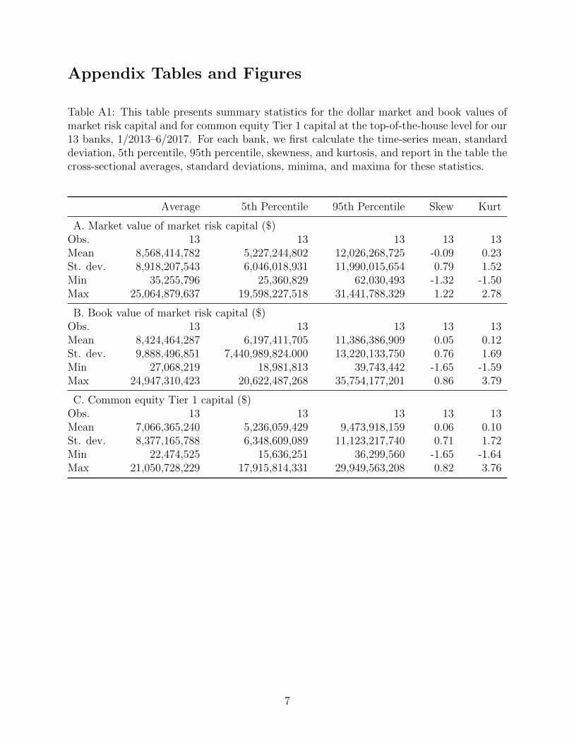
Appendix Tables and Figures
Table A1: This table presents summary statistics for the dollar market and book values ofmarket risk capital and for common equity Tier 1 capital at the top-of-the-house level for our13 banks, 1/2013–6/2017. For each bank, we first calculate the time-series mean, standarddeviation, 5th percentile, 95th percentile, skewness, and kurtosis, and report in the table thecross-sectional averages, standard deviations, minima, and maxima for these statistics.
Average 5th Percentile 95th Percentile Skew Kurt
A. Market value of market risk capital ($)Obs. 13 13 13 13 13Mean 8,568,414,782 5,227,244,802 12,026,268,725 -0.09 0.23St. dev. 8,918,207,543 6,046,018,931 11,990,015,654 0.79 1.52Min 35,255,796 25,360,829 62,030,493 -1.32 -1.50Max 25,064,879,637 19,598,227,518 31,441,788,329 1.22 2.78
B. Book value of market risk capital ($)Obs. 13 13 13 13 13Mean 8,424,464,287 6,197,411,705 11,386,386,909 0.05 0.12St. dev. 9,888,496,851 7,440,989,824.000 13,220,133,750 0.76 1.69Min 27,068,219 18,981,813 39,743,442 -1.65 -1.59Max 24,947,310,423 20,622,487,268 35,754,177,201 0.86 3.79
C. Common equity Tier 1 capital ($)Obs. 13 13 13 13 13Mean 7,066,365,240 5,236,059,429 9,473,918,159 0.06 0.10St. dev. 8,377,165,788 6,348,609,089 11,123,217,740 0.71 1.72Min 22,474,525 15,636,251 36,299,560 -1.65 -1.64Max 21,050,728,229 17,915,814,331 29,949,563,208 0.82 3.76
7
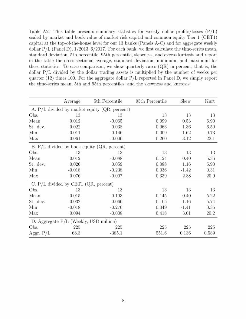
Table A2: This table presents summary statistics for weekly dollar profits/losses (P/L)scaled by market and book value of market risk capital and common equity Tier 1 (CET1)capital at the top-of-the-house level for our 13 banks (Panels A-C) and for aggregate weeklydollar P/L (Panel D), 1/2013–6/2017. For each bank, we first calculate the time-series mean,standard deviation, 5th percentile, 95th percentile, skewness, and excess kurtosis and reportin the table the cross-sectional average, standard deviation, minimum, and maximum forthese statistics. To ease comparison, we show quarterly rates (QR) in percent, that is, thedollar P/L divided by the dollar trading assets is multiplied by the number of weeks perquarter (12) times 100. For the aggregate dollar P/L reported in Panel D, we simply reportthe time-series mean, 5th and 95th percentiles, and the skewness and kurtosis.
Average 5th Percentile 95th Percentile Skew Kurt
A. P/L divided by market equity (QR, percent)Obs. 13 13 13 13 13Mean 0.012 -0.065 0.099 0.53 6.90St. dev. 0.022 0.038 0.063 1.36 6.50Min -0.011 -0.146 0.009 -1.62 0.73Max 0.061 -0.006 0.260 3.12 22.1
B. P/L divided by book equity (QR, percent)Obs. 13 13 13 13 13Mean 0.012 -0.088 0.124 0.40 5.36St. dev. 0.026 0.059 0.088 1.16 5.90Min -0.018 -0.238 0.036 -1.42 0.31Max 0.076 -0.007 0.339 2.88 20.9
C. P/L divided by CET1 (QR, percent)Obs. 13 13 13 13 13Mean 0.015 -0.103 0.145 0.40 5.22St. dev. 0.032 0.066 0.105 1.16 5.74Min -0.018 -0.276 0.049 -1.41 0.36Max 0.094 -0.008 0.418 3.01 20.2
D. Aggregate P/L (Weekly, USD million)Obs. 225 225 225 225 225Aggr. P/L 68.3 -385.1 551.6 0.136 0.589
8
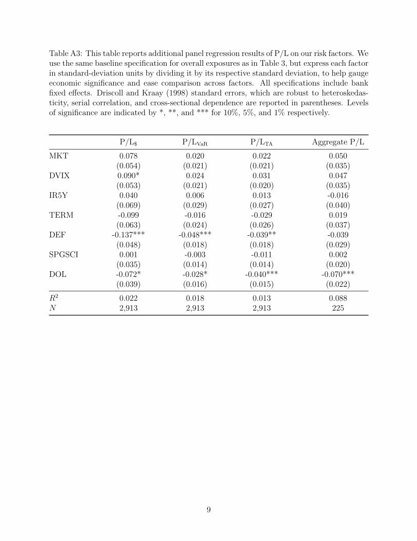
Table A3: This table reports additional panel regression results of P/L on our risk factors. Weuse the same baseline specification for overall exposures as in Table 3, but express each factorin standard-deviation units by dividing it by its respective standard deviation, to help gaugeeconomic significance and ease comparison across factors. All specifications include bankfixed effects. Driscoll and Kraay (1998) standard errors, which are robust to heteroskedas-ticity, serial correlation, and cross-sectional dependence are reported in parentheses. Levelsof significance are indicated by *, **, and *** for 10%, 5%, and 1% respectively.
P/L$ P/LVaR P/LTA Aggregate P/L
MKT 0.078 0.020 0.022 0.050(0.054) (0.021) (0.021) (0.035)
DVIX 0.090* 0.024 0.031 0.047(0.053) (0.021) (0.020) (0.035)
IR5Y 0.040 0.006 0.013 -0.016(0.069) (0.029) (0.027) (0.040)
TERM -0.099 -0.016 -0.029 0.019(0.063) (0.024) (0.026) (0.037)
DEF -0.137*** -0.048*** -0.039** -0.039(0.048) (0.018) (0.018) (0.029)
SPGSCI 0.001 -0.003 -0.011 0.002(0.035) (0.014) (0.014) (0.020)
DOL -0.072* -0.028* -0.040*** -0.070***(0.039) (0.016) (0.015) (0.022)
R2 0.022 0.018 0.013 0.088N 2,913 2,913 2,913 225
9

Table A4: This table reports additional panel regression results of P/L on standardized riskfactors interacted with the Volcker indicator variable, which takes the value of one after theintroduction of the Volcker rule in April 2014 and zero otherwise. We use the same baselinespecification for the change in exposures after Volcker as in Table 4, but express each factorin standard-deviation units by dividing it by its respective standard deviation, to help gaugeeconomic significance and ease comparison across factors. All specifications includes bankfixed effects. Driscoll and Kraay (1998) standard errors, which are robust to heteroskedas-ticity, serial correlation, and cross-sectional dependence are reported in parentheses. Levelsof significance are indicated by *, **, and *** for 10%, 5%, and 1% respectively.
P/L$ P/LVaR P/LTA Aggregate P/L
Volcker -0.077 -0.038 -0.018 -0.116*(0.137) (0.044) (0.061) (0.070)
MKT 0.333** 0.111*** 0.122* 0.167**(0.138) (0.042) (0.062) (0.079)
DVIX 0.354 0.110* 0.160 0.129(0.219) (0.062) (0.100) (0.102)
IR5Y 0.164 0.050 0.047 -0.009(0.170) (0.050) (0.077) (0.084)
TERM -0.300** -0.076* -0.103* -0.054(0.137) (0.041) (0.061) (0.071)
DEF -0.074 -0.018 -0.033 0.001(0.110) (0.035) (0.043) (0.064)
SPGSCI 0.079 0.022 0.056* 0.040(0.075) (0.024) (0.030) (0.058)
DOL -0.101 -0.033 -0.039 -0.107**(0.094) (0.030) (0.038) (0:052)
Volcker × MKT -0.371** -0.135*** -0.152** -0.196**(0.148) (0.047) (0.065) (0.086)
Volcker × DVIX -0.352 -0.118* -0.178* -0.136(0.224) (0.066) (0.102) (0.106)
Volcker × IR5Y -0.141 -0.049 -0.011 0.003(0.186) (0.060) (0.084) (0.095)
Volcker × TERM 0.260* 0.070 0.066 0.085(0.150) (0.050) (0.065) (0.081)
Volcker × DEF -0.099 -0.050 -0.028 -0.062(0.118) (0.040) (0.046) (0.069)
Volcker × SPGSCI -0.097 -0.032 -0.067** -0.046(0.083) (0.028) (0.033) (0.061)
Volcker × DOL 0.010 -0.006 0.025 0.017(0.102) (0.035) (0.041) (0.056)
R2 0.040 0.033 0.023 0.189N 2,913 2,913 2,913 225
10

Table A5: This table reports additional panel regression results of P/L on our risk factorsinteracted with the Volcker indicator variable, which takes the value of one after the in-troduction of the Volcker rule in April 2014 and zero otherwise. We use the same baselinespecification for the change in exposures after Volcker as in Table 4, but report results forfour alternative scalings of P/L, market and book value of market risk capital (ME andBE), common equity Tier 1 (CET1) capital, and weekly trading assets from FR 2644 (FR).The specification includes bank fixed effects. Driscoll and Kraay (1998) standard errors,which are robust to heteroskedasticity, serial correlation, and cross-sectional dependence arereported in parentheses. Levels of significance are indicated by *, **, and *** for 10%, 5%,and 1% respectively.
PLME PLBE PLCET1 PLFR
Volcker -0.001* -0.001 -0.001 -0.054(0.001) (0.001) (0.001) (0.051)
MKT 0.104** 0.118** 0.142** 6.865**(0.041) (0.048) (0.056) (3.105)
DVIX 0.001 0.001 0.001 0.044(0.0004) (0.0004) (0.0005) (0.029)
IR5Y 0.007 0.011 0.013 0.579(0.010) (0.012) (0.014) (0.595)
TERM -0.012 -0.017 -0.019 -1.297**(0.008) (0.011) (0.012) (0.590)
DEF 0.008 0.004 0.005 -0.814(0.015) (0.016) (0.018) (0.797)
SPGSCI 0.024 0.027 0.030 1.184(0.019) (0.019) (0.022) (1.293)
DOL -0.064 -0.080 -0.092 -9.783**(0.059) (0.065) (0.076) (4.473)
Volcker × MKT -0.118*** -0.129** -0.154*** -8.088**(0.043) (0.051) (0.059) (3.457)
Volcker × DVIX -0.001 -0.001 -0.001 -0.045(0.0004) (0.0004) (0.0005) (0.030)
Volcker × IR5Y -0.004 -0.008 -0.009 -0.466(0.010) (0.012) (0.014) (0.681)
Volcker × TERM 0.010 0.012 0.015 1.219*(0.009) (0.011) (0.013) (0.666)
Volcker × DEF -0.021 -0.020 -0.025 -0.045(0.016) (0.016) (0.019) (0.884)
Volcker × SPGSCI -0.030 -0.036* -0.040* -1.879(0.019) (0.020) (0.023) (1.410)
Volcker × DOL 0.017 0.049 0.056 3.782(0.063) (0.069) (0.082) (4.980)
R2 0.031 0.017 0.018 0.026N 2,913 2,913 2,913 2,452
11
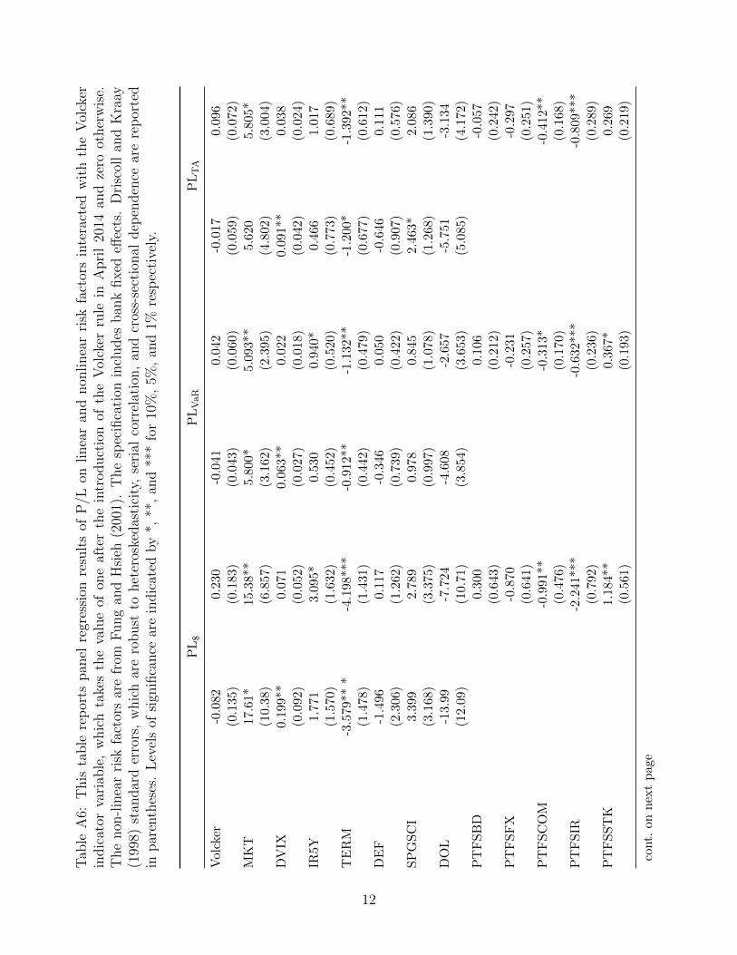
Tab
leA
6:T
his
table
rep
orts
pan
elre
gres
sion
resu
lts
ofP
/Lon
linea
ran
dnon
linea
rri
skfa
ctor
sin
tera
cted
wit
hth
eV
olck
erin
dic
ator
vari
able
,w
hic
hta
kes
the
valu
eof
one
afte
rth
ein
troduct
ion
ofth
eV
olck
erru
lein
Apri
l20
14an
dze
root
her
wis
e.T
he
non
-lin
ear
risk
fact
ors
are
from
Fung
and
Hsi
eh(2
001)
.T
he
spec
ifica
tion
incl
udes
ban
kfixed
effec
ts.
Dri
scol
lan
dK
raay
(199
8)st
andar
der
rors
,w
hic
har
ero
bust
tohet
eros
kedas
tici
ty,
seri
alco
rrel
atio
n,
and
cros
s-se
ctio
nal
dep
enden
cear
ere
por
ted
inpar
enth
eses
.L
evel
sof
sign
ifica
nce
are
indic
ated
by
*,**
,an
d**
*fo
r10
%,
5%,
and
1%re
spec
tive
ly.
PL$
PLVaR
PLTA
Volcker
-0.082
0.23
0-0.041
0.04
2-0.017
0.09
6(0.135
)(0.183
)(0.043
)(0.060
)(0.059
)(0.072
)MKT
17.61*
15.38*
*5.80
0*5.09
3**
5.62
05.80
5*(10.38
)(6.857
)(3.162
)(2.395
)(4.802
)(3.004
)DVIX
0.19
9**
0.07
10.06
3**
0.02
20.09
1**
0.03
8(0.092
)(0.052
)(0.027
)(0.018
)(0.042
)(0.024
)IR
5Y1.771
3.09
5*0.53
00.94
0*0.46
61.01
7(1.570
)(1.632
)(0.452
)(0.520
)(0.773
)(0.689
)TERM
-3.579
***
-4.198
***
-0.912
**-1.132
**-1.200
*-1.392
**(1.478
)(1.431
)(0.442
)(0.479
)(0.677
)(0.612
)DEF
-1.496
0.11
7-0.346
0.05
0-0.646
0.11
1(2.306
)(1.262
)(0.739
)(0.422
)(0.907
)(0.576
)SPGSCI
3.39
92.78
90.97
80.84
52.46
3*2.08
6(3.168
)(3.375
)(0.997
)(1.078
)(1.268
)(1.390
)DOL
-13.99
-7.724
-4.608
-2.657
-5.751
-3.134
(12.09
)(10.71
)(3.854
)(3.653
)(5.085
)(4.172
)PTFSBD
0.30
00.10
6-0.057
(0.643
)(0.212
)(0.242
)PTFSFX
-0.870
-0.231
-0.297
(0.641
)(0.257
)(0.251
)PTFSCOM
-0.991
**-0.313
*-0.412
**(0.476
)(0.170
)(0.168
)PTFSIR
-2.241
***
-0.632
***
-0.809
***
(0.792
)(0.236
)(0.289
)PTFSSTK
1.18
4**
0.36
7*0.26
9(0.561
)(0.193
)(0.219
)
cont.onnextpage
12
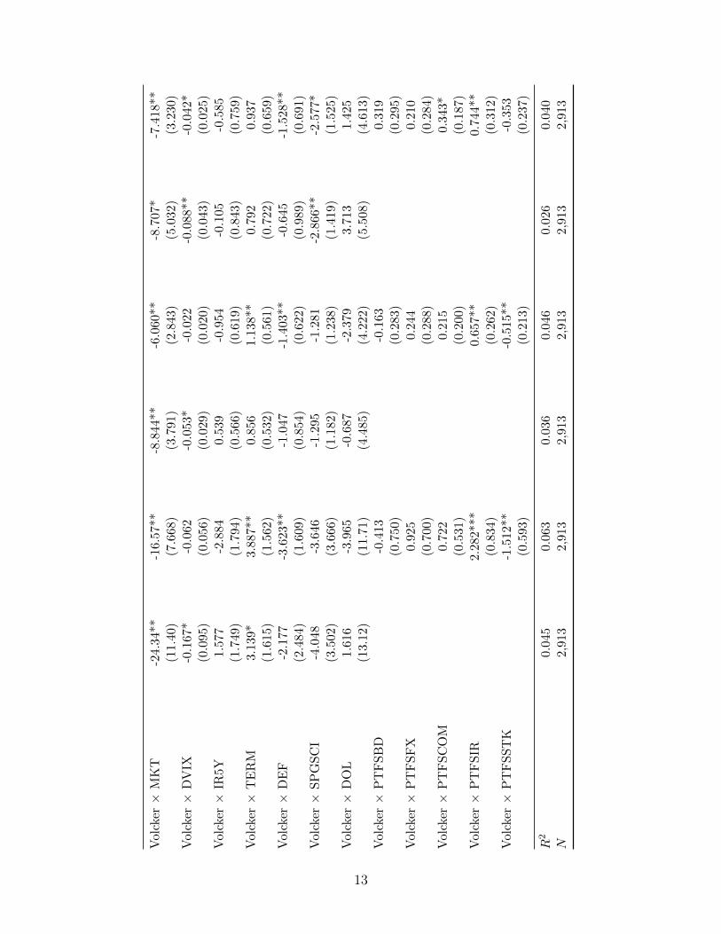
Volcker×
MKT
-24.34
**
-16.57
**-8.844
**-6.060
**-8.707
*-7.418
**(11.40)
(7.668
)(3.791
)(2.843
)(5.032
)(3.230
)Volcker×
DVIX
-0.167
*-0.062
-0.053
*-0.022
-0.088
**-0.042
*(0.095)
(0.056
)(0.029
)(0.020
)(0.043
)(0.025
)Volcker×
IR5Y
1.577
-2.884
0.53
9-0.954
-0.105
-0.585
(1.749)
(1.794
)(0.566
)(0.619
)(0.843
)(0.759
)Volcker×
TERM
3.139
*3.88
7**
0.85
61.13
8**
0.79
20.93
7(1.615)
(1.562
)(0.532
)(0.561
)(0.722
)(0.659
)Volcker×
DEF
-2.177
-3.623
**-1.047
-1.403
**-0.645
-1.528
**(2.484)
(1.609
)(0.854
)(0.622
)(0.989
)(0.691
)Volcker×
SPGSCI
-4.048
-3.646
-1.295
-1.281
-2.866
**-2.577
*(3.502)
(3.666
)(1.182
)(1.238
)(1.419
)(1.525
)Volcker×
DOL
1.616
-3.965
-0.687
-2.379
3.71
31.42
5(13.12)
(11.71
)(4.485
)(4.222
)(5.508
)(4.613
)Volcker×
PTFSBD
-0.413
-0.163
0.31
9(0.750
)(0.283
)(0.295
)Volcker×
PTFSFX
0.92
50.24
40.21
0(0.700
)(0.288
)(0.284
)Volcker×
PTFSCOM
0.72
20.21
50.34
3*(0.531
)(0.200
)(0.187
)Volcker×
PTFSIR
2.28
2***
0.65
7**
0.74
4**
(0.834
)(0.262
)(0.312
)Volcker×
PTFSSTK
-1.512
**-0.515
**-0.353
(0.593
)(0.213
)(0.237
)
R2
0.045
0.06
30.03
60.04
60.02
60.04
0N
2,913
2,91
32,91
32,91
32,91
32,91
3
13
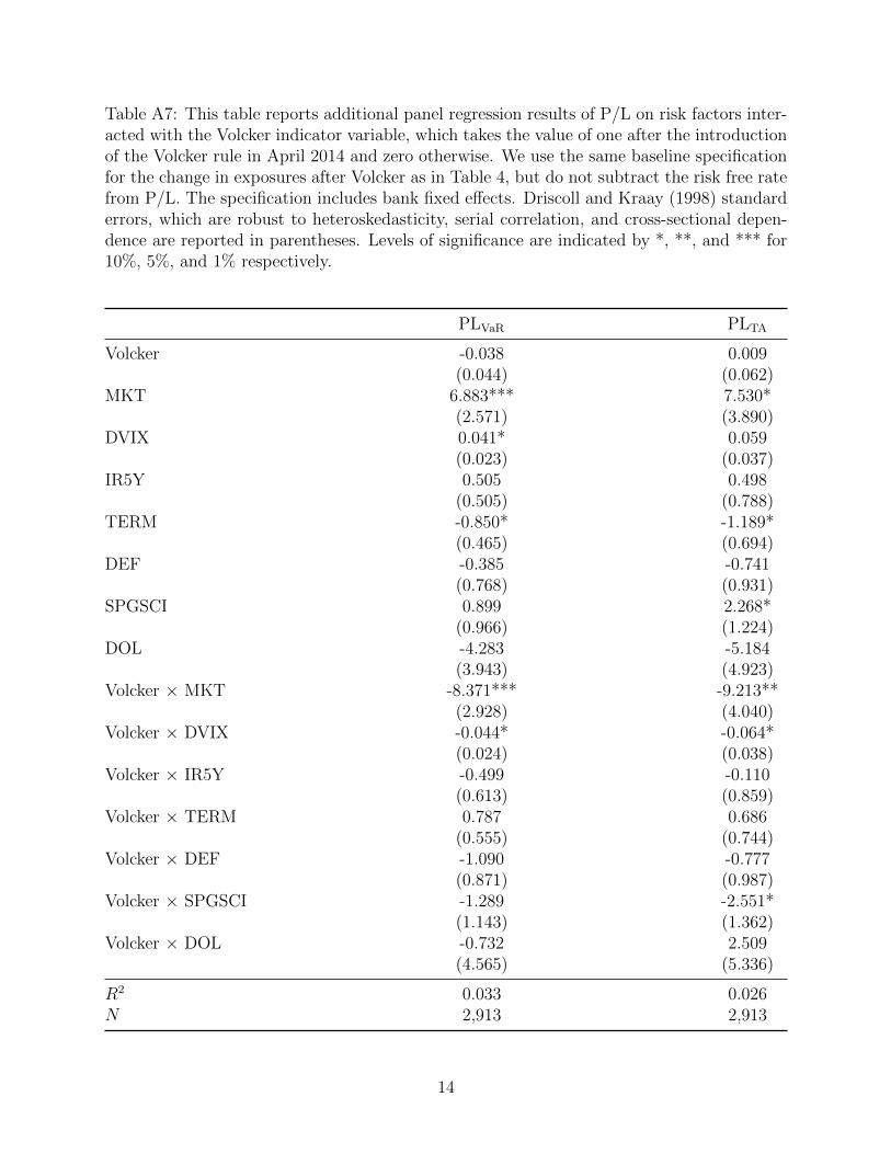
Table A7: This table reports additional panel regression results of P/L on risk factors inter-acted with the Volcker indicator variable, which takes the value of one after the introductionof the Volcker rule in April 2014 and zero otherwise. We use the same baseline specificationfor the change in exposures after Volcker as in Table 4, but do not subtract the risk free ratefrom P/L. The specification includes bank fixed effects. Driscoll and Kraay (1998) standarderrors, which are robust to heteroskedasticity, serial correlation, and cross-sectional depen-dence are reported in parentheses. Levels of significance are indicated by *, **, and *** for10%, 5%, and 1% respectively.
PLVaR PLTA
Volcker -0.038 0.009(0.044) (0.062)
MKT 6.883*** 7.530*(2.571) (3.890)
DVIX 0.041* 0.059(0.023) (0.037)
IR5Y 0.505 0.498(0.505) (0.788)
TERM -0.850* -1.189*(0.465) (0.694)
DEF -0.385 -0.741(0.768) (0.931)
SPGSCI 0.899 2.268*(0.966) (1.224)
DOL -4.283 -5.184(3.943) (4.923)
Volcker × MKT -8.371*** -9.213**(2.928) (4.040)
Volcker × DVIX -0.044* -0.064*(0.024) (0.038)
Volcker × IR5Y -0.499 -0.110(0.613) (0.859)
Volcker × TERM 0.787 0.686(0.555) (0.744)
Volcker × DEF -1.090 -0.777(0.871) (0.987)
Volcker × SPGSCI -1.289 -2.551*(1.143) (1.362)
Volcker × DOL -0.732 2.509(4.565) (5.336)
R2 0.033 0.026N 2,913 2,913
14
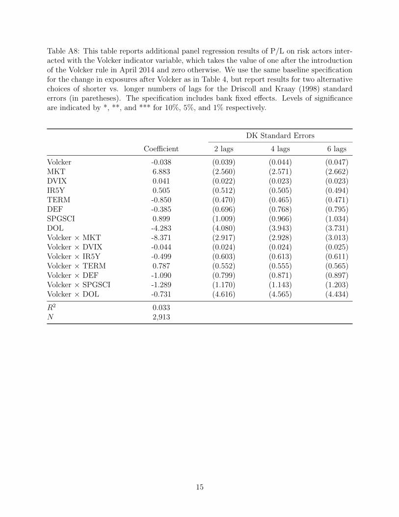
Table A8: This table reports additional panel regression results of P/L on risk actors inter-acted with the Volcker indicator variable, which takes the value of one after the introductionof the Volcker rule in April 2014 and zero otherwise. We use the same baseline specificationfor the change in exposures after Volcker as in Table 4, but report results for two alternativechoices of shorter vs. longer numbers of lags for the Driscoll and Kraay (1998) standarderrors (in paretheses). The specification includes bank fixed effects. Levels of significanceare indicated by *, **, and *** for 10%, 5%, and 1% respectively.
DK Standard Errors
Coefficient 2 lags 4 lags 6 lags
Volcker -0.038 (0.039) (0.044) (0.047)MKT 6.883 (2.560) (2.571) (2.662)DVIX 0.041 (0.022) (0.023) (0.023)IR5Y 0.505 (0.512) (0.505) (0.494)TERM -0.850 (0.470) (0.465) (0.471)DEF -0.385 (0.696) (0.768) (0.795)SPGSCI 0.899 (1.009) (0.966) (1.034)DOL -4.283 (4.080) (3.943) (3.731)Volcker × MKT -8.371 (2.917) (2.928) (3.013)Volcker × DVIX -0.044 (0.024) (0.024) (0.025)Volcker × IR5Y -0.499 (0.603) (0.613) (0.611)Volcker × TERM 0.787 (0.552) (0.555) (0.565)Volcker × DEF -1.090 (0.799) (0.871) (0.897)Volcker × SPGSCI -1.289 (1.170) (1.143) (1.203)Volcker × DOL -0.731 (4.616) (4.565) (4.434)
R2 0.033N 2,913
15
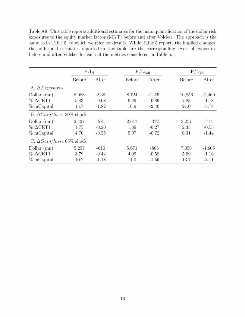
Table A9: This table reports additional estimates for the main quantification of the dollar riskexposures to the equity market factor (MKT) before and after Volcker. The approach is thesame as in Table 5, to which we refer for details. While Table 5 reports the implied changes,the additional estimates reported in this table are the corresponding levels of exposuresbefore and after Volcker for each of the metrics considered in Table 5.
P/L$ P/LVaR P/LTA
Before After Before After Before After
A. ∆Exposures
Dollar (mn) 8,088 -938 8,724 -1,239 10,856 -2,469% ∆CET1 5.83 -0.68 6.29 -0.89 7.83 -1.78% mCapital 15.7 -1.82 16.9 -2.40 21.0 -4.78
B. ∆Gain/loss: 30% shock
Dollar (mn) 2,427 -281 2,617 -372 3,257 -741% ∆CET1 1.75 -0.20 1.89 -0.27 2.35 -0.53% mCapital 4.70 -0.55 5.07 -0.72 6.31 -1.44
C. ∆Gain/loss: 65% shock
Dollar (mn) 5,257 -610 5,671 -805 7,056 -1,605% ∆CET1 3.79 -0.44 4.09 -0.58 5.09 -1.16% mCapital 10.2 -1.18 11.0 -1.56 13.7 -3.11
16
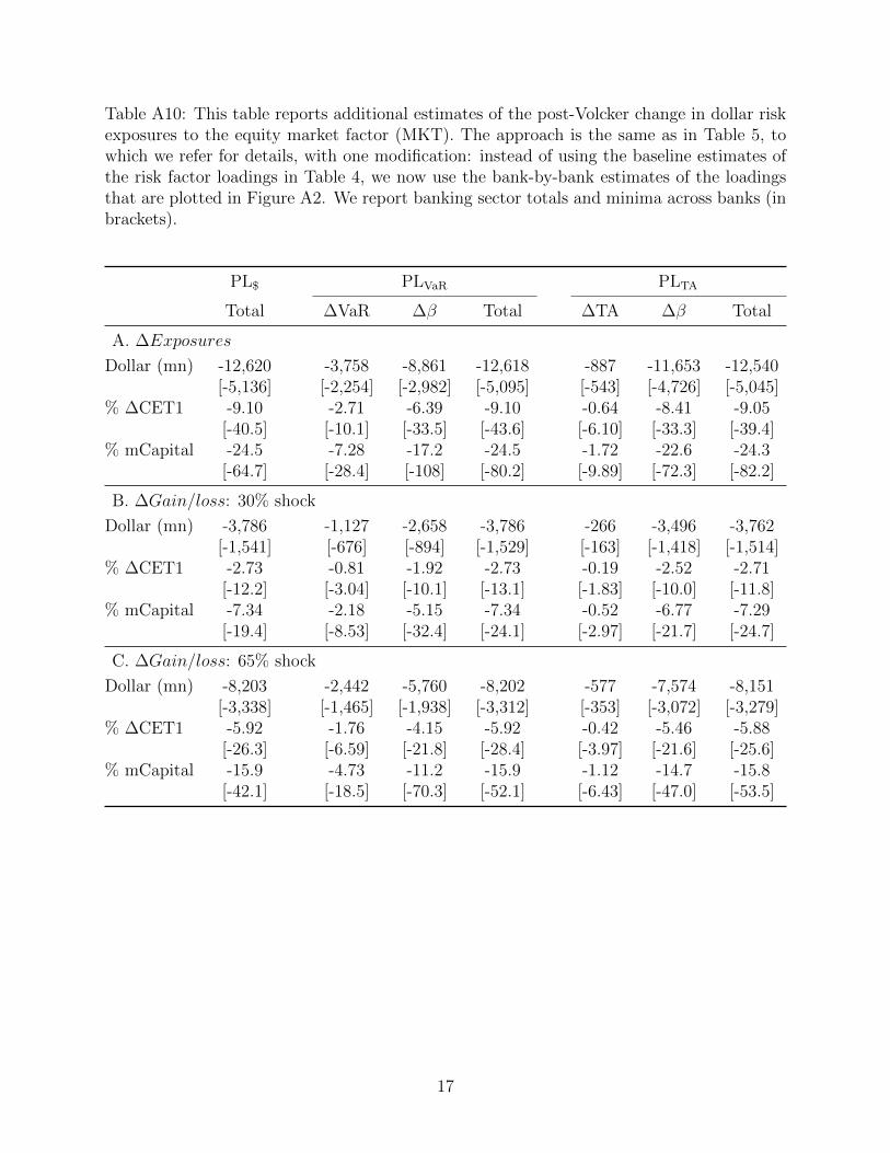
Table A10: This table reports additional estimates of the post-Volcker change in dollar riskexposures to the equity market factor (MKT). The approach is the same as in Table 5, towhich we refer for details, with one modification: instead of using the baseline estimates ofthe risk factor loadings in Table 4, we now use the bank-by-bank estimates of the loadingsthat are plotted in Figure A2. We report banking sector totals and minima across banks (inbrackets).
PL$ PLVaR PLTA
Total ∆VaR ∆β Total ∆TA ∆β Total
A. ∆Exposures
Dollar (mn) -12,620 -3,758 -8,861 -12,618 -887 -11,653 -12,540[-5,136] [-2,254] [-2,982] [-5,095] [-543] [-4,726] [-5,045]
% ∆CET1 -9.10 -2.71 -6.39 -9.10 -0.64 -8.41 -9.05[-40.5] [-10.1] [-33.5] [-43.6] [-6.10] [-33.3] [-39.4]
% mCapital -24.5 -7.28 -17.2 -24.5 -1.72 -22.6 -24.3[-64.7] [-28.4] [-108] [-80.2] [-9.89] [-72.3] [-82.2]
B. ∆Gain/loss: 30% shock
Dollar (mn) -3,786 -1,127 -2,658 -3,786 -266 -3,496 -3,762[-1,541] [-676] [-894] [-1,529] [-163] [-1,418] [-1,514]
% ∆CET1 -2.73 -0.81 -1.92 -2.73 -0.19 -2.52 -2.71[-12.2] [-3.04] [-10.1] [-13.1] [-1.83] [-10.0] [-11.8]
% mCapital -7.34 -2.18 -5.15 -7.34 -0.52 -6.77 -7.29[-19.4] [-8.53] [-32.4] [-24.1] [-2.97] [-21.7] [-24.7]
C. ∆Gain/loss: 65% shock
Dollar (mn) -8,203 -2,442 -5,760 -8,202 -577 -7,574 -8,151[-3,338] [-1,465] [-1,938] [-3,312] [-353] [-3,072] [-3,279]
% ∆CET1 -5.92 -1.76 -4.15 -5.92 -0.42 -5.46 -5.88[-26.3] [-6.59] [-21.8] [-28.4] [-3.97] [-21.6] [-25.6]
% mCapital -15.9 -4.73 -11.2 -15.9 -1.12 -14.7 -15.8[-42.1] [-18.5] [-70.3] [-52.1] [-6.43] [-47.0] [-53.5]
17
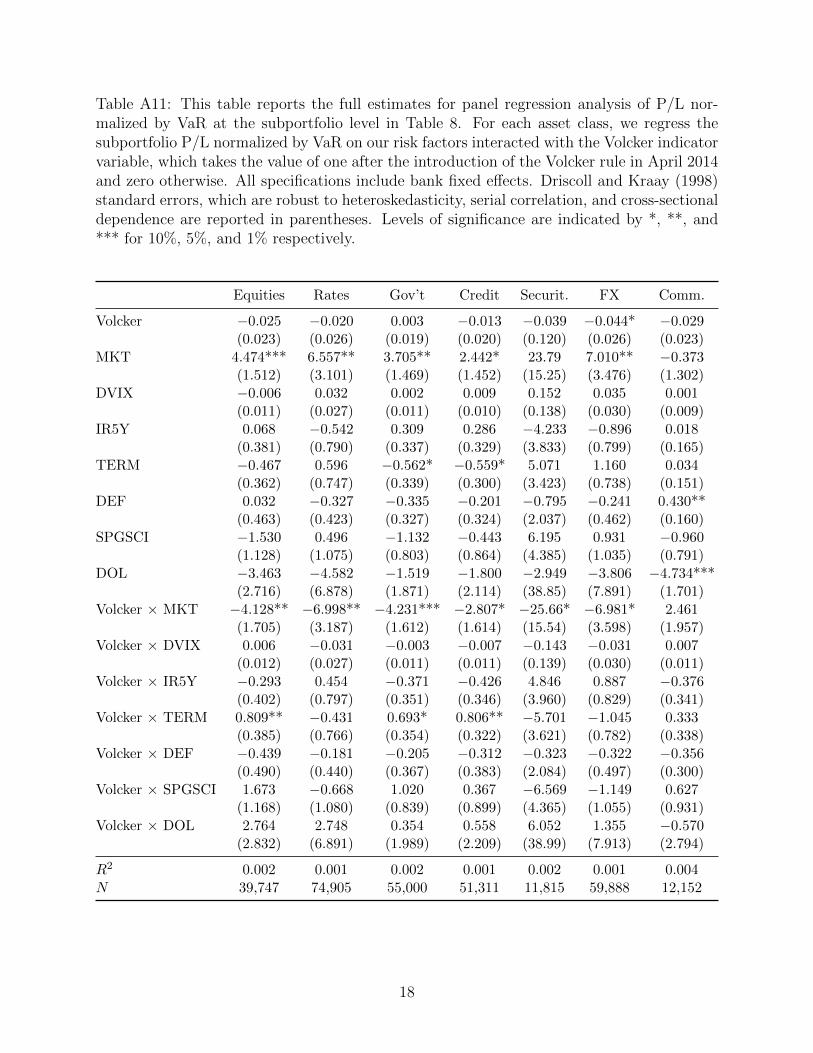
Table A11: This table reports the full estimates for panel regression analysis of P/L nor-malized by VaR at the subportfolio level in Table 8. For each asset class, we regress thesubportfolio P/L normalized by VaR on our risk factors interacted with the Volcker indicatorvariable, which takes the value of one after the introduction of the Volcker rule in April 2014and zero otherwise. All specifications include bank fixed effects. Driscoll and Kraay (1998)standard errors, which are robust to heteroskedasticity, serial correlation, and cross-sectionaldependence are reported in parentheses. Levels of significance are indicated by *, **, and*** for 10%, 5%, and 1% respectively.
Equities Rates Gov’t Credit Securit. FX Comm.
Volcker −0.025 −0.020 0.003 −0.013 −0.039 −0.044* −0.029(0.023) (0.026) (0.019) (0.020) (0.120) (0.026) (0.023)
MKT 4.474*** 6.557** 3.705** 2.442* 23.79 7.010** −0.373(1.512) (3.101) (1.469) (1.452) (15.25) (3.476) (1.302)
DVIX −0.006 0.032 0.002 0.009 0.152 0.035 0.001(0.011) (0.027) (0.011) (0.010) (0.138) (0.030) (0.009)
IR5Y 0.068 −0.542 0.309 0.286 −4.233 −0.896 0.018(0.381) (0.790) (0.337) (0.329) (3.833) (0.799) (0.165)
TERM −0.467 0.596 −0.562* −0.559* 5.071 1.160 0.034(0.362) (0.747) (0.339) (0.300) (3.423) (0.738) (0.151)
DEF 0.032 −0.327 −0.335 −0.201 −0.795 −0.241 0.430**(0.463) (0.423) (0.327) (0.324) (2.037) (0.462) (0.160)
SPGSCI −1.530 0.496 −1.132 −0.443 6.195 0.931 −0.960(1.128) (1.075) (0.803) (0.864) (4.385) (1.035) (0.791)
DOL −3.463 −4.582 −1.519 −1.800 −2.949 −3.806 −4.734***(2.716) (6.878) (1.871) (2.114) (38.85) (7.891) (1.701)
Volcker × MKT −4.128** −6.998** −4.231*** −2.807* −25.66* −6.981* 2.461(1.705) (3.187) (1.612) (1.614) (15.54) (3.598) (1.957)
Volcker × DVIX 0.006 −0.031 −0.003 −0.007 −0.143 −0.031 0.007(0.012) (0.027) (0.011) (0.011) (0.139) (0.030) (0.011)
Volcker × IR5Y −0.293 0.454 −0.371 −0.426 4.846 0.887 −0.376(0.402) (0.797) (0.351) (0.346) (3.960) (0.829) (0.341)
Volcker × TERM 0.809** −0.431 0.693* 0.806** −5.701 −1.045 0.333(0.385) (0.766) (0.354) (0.322) (3.621) (0.782) (0.338)
Volcker × DEF −0.439 −0.181 −0.205 −0.312 −0.323 −0.322 −0.356(0.490) (0.440) (0.367) (0.383) (2.084) (0.497) (0.300)
Volcker × SPGSCI 1.673 −0.668 1.020 0.367 −6.569 −1.149 0.627(1.168) (1.080) (0.839) (0.899) (4.365) (1.055) (0.931)
Volcker × DOL 2.764 2.748 0.354 0.558 6.052 1.355 −0.570(2.832) (6.891) (1.989) (2.209) (38.99) (7.913) (2.794)
R2 0.002 0.001 0.002 0.001 0.002 0.001 0.004N 39,747 74,905 55,000 51,311 11,815 59,888 12,152
18
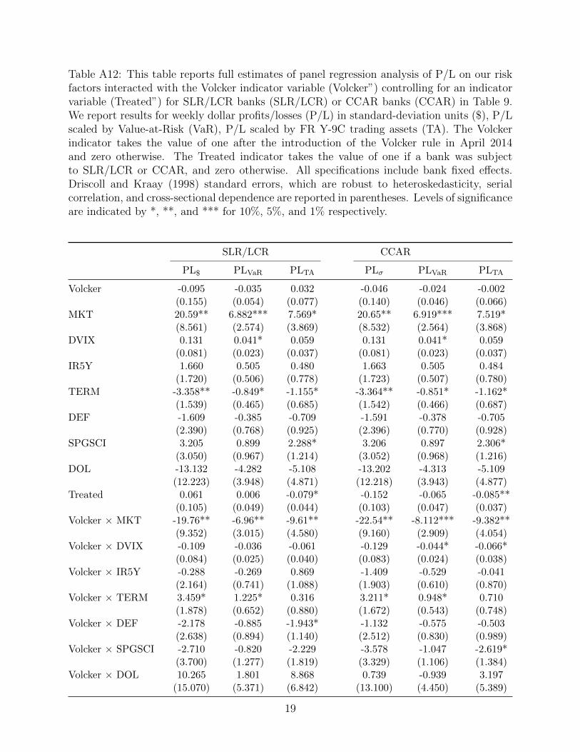
Table A12: This table reports full estimates of panel regression analysis of P/L on our riskfactors interacted with the Volcker indicator variable (Volcker”) controlling for an indicatorvariable (Treated”) for SLR/LCR banks (SLR/LCR) or CCAR banks (CCAR) in Table 9.We report results for weekly dollar profits/losses (P/L) in standard-deviation units ($), P/Lscaled by Value-at-Risk (VaR), P/L scaled by FR Y-9C trading assets (TA). The Volckerindicator takes the value of one after the introduction of the Volcker rule in April 2014and zero otherwise. The Treated indicator takes the value of one if a bank was subjectto SLR/LCR or CCAR, and zero otherwise. All specifications include bank fixed effects.Driscoll and Kraay (1998) standard errors, which are robust to heteroskedasticity, serialcorrelation, and cross-sectional dependence are reported in parentheses. Levels of significanceare indicated by *, **, and *** for 10%, 5%, and 1% respectively.
SLR/LCR CCAR
PL$ PLVaR PLTA PLσ PLVaR PLTA
Volcker -0.095 -0.035 0.032 -0.046 -0.024 -0.002(0.155) (0.054) (0.077) (0.140) (0.046) (0.066)
MKT 20.59** 6.882*** 7.569* 20.65** 6.919*** 7.519*(8.561) (2.574) (3.869) (8.532) (2.564) (3.868)
DVIX 0.131 0.041* 0.059 0.131 0.041* 0.059(0.081) (0.023) (0.037) (0.081) (0.023) (0.037)
IR5Y 1.660 0.505 0.480 1.663 0.505 0.484(1.720) (0.506) (0.778) (1.723) (0.507) (0.780)
TERM -3.358** -0.849* -1.155* -3.364** -0.851* -1.162*(1.539) (0.465) (0.685) (1.542) (0.466) (0.687)
DEF -1.609 -0.385 -0.709 -1.591 -0.378 -0.705(2.390) (0.768) (0.925) (2.396) (0.770) (0.928)
SPGSCI 3.205 0.899 2.288* 3.206 0.897 2.306*(3.050) (0.967) (1.214) (3.052) (0.968) (1.216)
DOL -13.132 -4.282 -5.108 -13.202 -4.313 -5.109(12.223) (3.948) (4.871) (12.218) (3.943) (4.877)
Treated 0.061 0.006 -0.079* -0.152 -0.065 -0.085**(0.105) (0.049) (0.044) (0.103) (0.047) (0.037)
Volcker × MKT -19.76** -6.96** -9.61** -22.54** -8.112*** -9.382**(9.352) (3.015) (4.580) (9.160) (2.909) (4.054)
Volcker × DVIX -0.109 -0.036 -0.061 -0.129 -0.044* -0.066*(0.084) (0.025) (0.040) (0.083) (0.024) (0.038)
Volcker × IR5Y -0.288 -0.269 0.869 -1.409 -0.529 -0.041(2.164) (0.741) (1.088) (1.903) (0.610) (0.870)
Volcker × TERM 3.459* 1.225* 0.316 3.211* 0.948* 0.710(1.878) (0.652) (0.880) (1.672) (0.543) (0.748)
Volcker × DEF -2.178 -0.885 -1.943* -1.132 -0.575 -0.503(2.638) (0.894) (1.140) (2.512) (0.830) (0.989)
Volcker × SPGSCI -2.710 -0.820 -2.229 -3.578 -1.047 -2.619*(3.700) (1.277) (1.819) (3.329) (1.106) (1.384)
Volcker × DOL 10.265 1.801 8.868 0.739 -0.939 3.197(15.070) (5.371) (6.842) (13.100) (4.450) (5.389)
19

Treated × MKT -5.106 -2.396 -0.037 -2.805 -1.610 -0.169(5.145) (2.339) (2.691) (4.983) (1.993) (1.557)
Treated × DVIX -0.028 -0.010 -0.006 -0.008 0.001 0.004(0.025) (0.012) (0.014) (0.025) (0.010) (0.007)
Treated × IR5Y -1.309 -0.216 -1.405** -0.156 0.107 -0.362(1.286) (0.583) (0.661) (0.738) (0.387) (0.268)
Treated × TERM -1.270 -0.818 0.550 -1.340 -0.723* 0.210(1.168) (0.527) (0.512) (0.901) (0.430) (0.301)
Treated × DEF -0.083 -0.347 1.782** -4.754*** -2.378*** -0.525(1.631) (0.750) (0.850) (1.441) (0.814) (0.426)
Treated × SPGSCI -2.344 -0.813 -0.611 -1.423 -0.997 -0.438(2.234) (0.992) (1.309) (1.416) (0.819) -0.438
Treated × DOL -9.185 -2.563 -8.198* 2.427 0.860 -0.169(8.738) (3.812) (4.247) (7.898) (3.532) (2.189)
R2 0.052 0.042 0.040 0.045 0.039 0.025N 2,913 2,913 2,913 2,913 2,913 2,913
20

Table A13: This table reports the full estimates for the diff-in-diff analysis of the reportingrequirement in Table 10. Specifically, we report panel regression results of P/L on our riskfactors interacted with the Reporting indicator variable, which takes the value of one if abank is subject to the Volcker-related metrics reporting obligation and zero otherwise. Wereport results for weekly dollar profits/losses (P/L) in standard-deviation units ($), P/Lscaled by Value-at-Risk (VaR), P/L scaled by FR Y-9C trading assets (TA). In additionto the baseline panel regression results, we report results of robustness analysis using anevent-time specification for a 24-month window around each reporting date (Event time) aswell as to including controls for weekly dummies (Week FE) and the full sample of 20 banks(Extended). Driscoll and Kraay (1998) standard errors, which are robust to heteroskedas-ticity, serial correlation, and cross-sectional dependence are reported in parentheses. Levelsof significance are indicated by *, **, and *** for 10%, 5%, and 1% respectively.
Baseline Event time
PL$ PLVaR PLTA Baseline Week FE Extended
Reporting -0.178 -0.094* -0.097*** -0.071** -0.084***(0.136) (0.053) (0.037) (0.028) (0.031)
MKT 9.423*** 2.749** 2.493 4.069*** 4.003***(3.365) (1.234) (1.564) (1.139) (1.375)
DVIX 0.053** 0.013* 0.013 0.004 -0.001(0.021) (0.007) (0.009) (0.006) (0.008)
IR5Y 1.090* 0.266 0.655* -0.336* -0.256(0.661) (0.234) (0.383) (0.186) (0.283)
TERM -1.924*** -0.445* -1.009*** 0.251 -0.038(0.720) (0.238) (0.380) (0.373) (0.408)
DEF -2.553** -0.779* -1.135** 0.856** 0.717*(1.253) (0.409) (0.565) (0.352) (0.382)
SPGSCI -0.730 -0.510 -0.033 -0.233 -0.030(1.482) (0.510) (0.759) (0.261) (0.303)
DOL -0.753 0.517 0.246 -1.858 -3.370(5.500) (2.087) (2.565) (2.650) (3.344)
21
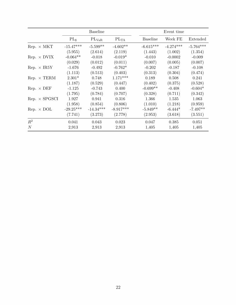
Baseline Event time
PL$ PLVaR PLTA Baseline Week FE Extended
Rep. × MKT -15.47*** -5.599** -4.602** -6.615*** -4.274*** -5.764***(5.955) (2.614) (2.119) (1.443) (1.002) (1.354)
Rep. × DVIX -0.064** -0.018 -0.019* -0.010 -0.0002 -0.009(0.029) (0.012) (0.011) (0.007) (0.005) (0.007)
Rep. × IR5Y -1.676 -0.492 -0.762* -0.202 -0.187 -0.108(1.113) (0.513) (0.403) (0.313) (0.304) (0.474)
Rep. × TERM 2.301* 0.748 1.171*** 0.189 0.508 0.241(1.187) (0.529) (0.447) (0.402) (0.375) (0.528)
Rep. × DEF -1.125 -0.743 0.400 -0.699** -0.408 -0.604*(1.795) (0.784) (0.707) (0.328) (0.711) (0.342)
Rep. × SPGSCI 1.927 0.941 0.316 1.366 1.535 1.063(1.958) (0.854) (0.806) (1.010) (1.218) (0.959)
Rep. × DOL -29.25*** -14.34*** -8.917*** -5.849** -6.444* -7.497**(7.741) (3.273) (2.778) (2.953) (3.618) (3.551)
R2 0.041 0.043 0.023 0.047 0.385 0.051N 2,913 2,913 2,913 1,405 1,405 1,405
22
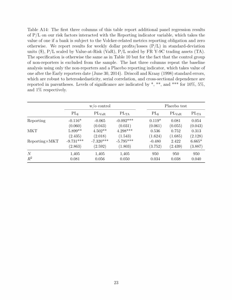
Table A14: The first three columns of this table report additional panel regression resultsof P/L on our risk factors interacted with the Reporting indicator variable, which takes thevalue of one if a bank is subject to the Volcker-related metrics reporting obligation and zerootherwise. We report results for weekly dollar profits/losses (P/L) in standard-deviationunits ($), P/L scaled by Value-at-Risk (VaR), P/L scaled by FR Y-9C trading assets (TA).The specification is otherwise the same as in Table 10 but for the fact that the control groupof non-reporters is excluded from the sample. The last three columns repeat the baselineanalysis using only the non-reporters and a Placebo reporting indicator, which takes value ofone after the Early reporters date (June 30, 2014). Driscoll and Kraay (1998) standard errors,which are robust to heteroskedasticity, serial correlation, and cross-sectional dependence arereported in parentheses. Levels of significance are indicated by *, **, and *** for 10%, 5%,and 1% respectively.
w/o control Placebo test
PL$ PLVaR PLTA PL$ PLVaR PLTA
Reporting -0.116* -0.065 -0.092*** 0.119* 0.081 0.054(0.060) (0.043) (0.031) (0.061) (0.055) (0.043)
MKT 5.899** 4.502** 4.298*** 0.536 0.752 0.313(2.435) (2.018) (1.543) (1.624) (1.685) (2.128)
Reporting×MKT -9.731*** -7.320*** -5.795*** -0.480 2.422 6.665*(2.863) (2.592) (1.803) (3.752) (2.439) (3.887)
N 1,405 1,405 1,405 950 950 950R2 0.081 0.056 0.050 0.034 0.038 0.040
23
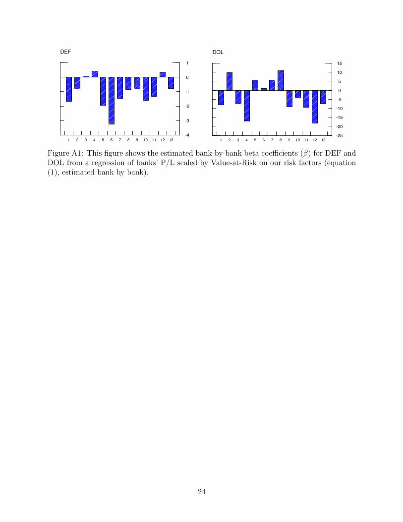
-0.06
-0.04
-0.02
0.00
0.02
0.04
0.06
DVIX
1 2 3 4 5 6 7 8 9 10 11 12 13-2.0
-1.5
-1.0
-0.5
0.0
0.5
1.0
1.5
2.0
IR.5Y
1 2 3 4 5 6 7 8 9 10 11 12 13
-3
-2
-1
0
1
2
TERM
1 2 3 4 5 6 7 8 9 10 11 12 13-4
-3
-2
-1
0
1
DEF
1 2 3 4 5 6 7 8 9 10 11 12 13
-3
-2
-1
0
1
2
3
SPGSCI
1 2 3 4 5 6 7 8 9 10 11 12 13-25
-20
-15
-10
-5
0
5
10
15
DOL
1 2 3 4 5 6 7 8 9 10 11 12 13
Figure A1: This figure shows the estimated bank-by-bank beta coefficients (β) for DEF andDOL from a regression of banks’ P/L scaled by Value-at-Risk on our risk factors (equation(1), estimated bank by bank).
24
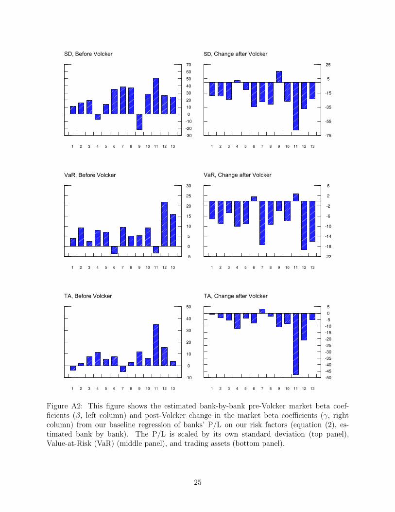
-30-20-100
10203040506070
SD, Before Volcker
1 2 3 4 5 6 7 8 9 10 11 12 13
-75
-55
-35
-15
5
25
SD, Change after Volcker
1 2 3 4 5 6 7 8 9 10 11 12 13
-5
0
5
10
15
20
25
30
VaR, Before Volcker
1 2 3 4 5 6 7 8 9 10 11 12 13
-22
-18
-14
-10
-6
-2
2
6
VaR, Change after Volcker
1 2 3 4 5 6 7 8 9 10 11 12 13
-10
0
10
20
30
40
50
TA, Before Volcker
1 2 3 4 5 6 7 8 9 10 11 12 13
-50-45-40-35-30-25-20-15-10-505
TA, Change after Volcker
1 2 3 4 5 6 7 8 9 10 11 12 13
Figure A2: This figure shows the estimated bank-by-bank pre-Volcker market beta coef-ficients (β, left column) and post-Volcker change in the market beta coefficients (γ, rightcolumn) from our baseline regression of banks’ P/L on our risk factors (equation (2), es-timated bank by bank). The P/L is scaled by its own standard deviation (top panel),Value-at-Risk (VaR) (middle panel), and trading assets (bottom panel).
25
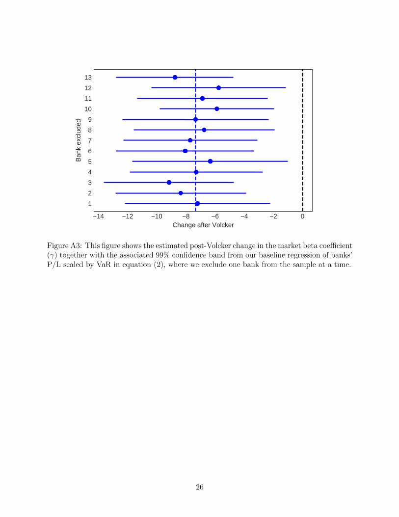
14 12 10 8 6 4 2 0Change after Volcker
1
2
3
4
5
6
7
8
9
10
11
12
13B
ank
excl
uded
Figure A3: This figure shows the estimated post-Volcker change in the market beta coefficient(γ) together with the associated 99% confidence band from our baseline regression of banks’P/L scaled by VaR in equation (2), where we exclude one bank from the sample at a time.
26

0.00.10.20.30.40.50.60.70.80.91.0
2013 2014 2015 2016 2017
Cumulative structural break frequencies
0.00.10.20.30.40.50.60.70.80.91.0
House (right axis)Subportfolio (left axis)
Figure A4: This figure plots the cumulative frequency of structural brakes in the sensitivityof the P/L normalized by VaR to the market return (MKT). We report results at the top-of-the-house level (line) and at the subportfolio level (bars). See Appendix A.5 for details.
27
Recommended


![A Comparison of the US and European Shadow Banking Systems ... · Definitions • Mculley ~ î ì ì ó : ^unlike regulated banks […], unregulated shadow banks fund themselves with](https://img.pdfslide.net/doc/110x75/5e37ea71309dfc2a7113eb46/a-comparison-of-the-us-and-european-shadow-banking-systems-definitions-a-mculley.jpg)