Bayesian analysis of the neuromagnetic inverse
problem with `p-norm priors
Toni Auranen,a,∗ Aapo Nummenmaa,a Matti S. Hämäläinen,b
Iiro P. Jääskeläinen,a,b Jouko Lampinen,a Aki Vehtari,a and Mikko Samsa
aLaboratory of Computational Engineering, Helsinki University of Technology, Espoo, Finland
bMassachusetts General Hospital – Massachusetts Institute of Technology – Harvard Medical School,
Athinoula A. Martinos Center for Biomedical Imaging, Charlestown, MA, USA
3rd December 2004; Submitted to NeuroImage
3rd February 2005; Revised and Resubmitted to NeuroImage
* Corresponding author. Group of Cognitive Science and Technology, Laboratory of Computational
Engineering, Helsinki University of Technology, P.O. Box 9203, 02015 HUT, Finland. Fax: +358-9-451
4830. Tel: +358-9-451 4834. E-mail address: [email protected] (T. Auranen)
1
Magnetoencephalography (MEG) allows millisecond-scale non-invasive
measurement of magnetic fields generated by neural currents in the brain. How-
ever, localization of the underlying current sources is ambiguous due to the so-called
inverse problem. The most widely used source localization methods (i.e., minimum-
norm and minimum-current estimates (MNE and MCE), and equivalent current
dipole (ECD) fitting) require ad hoc determination of the cortical current distribu-
tion (`2-, `1-norm priors, and point-sized dipolar, respectively). In this article, we
perform a Bayesian analysis of the MEG inverse problem with ` p-norm priors for
the current sources. This way, we circumvent the arbitrary choice between `1- and
`2-norm prior, which is instead rendered automatically based on the data. By obtain-
ing numerical samples from the joint posterior probability distribution of the source
current parameters and model hyperparameters (such as the `p-norm order p) us-
ing Markov chain Monte Carlo (MCMC) methods we calculated the spatial inverse
estimates as expectation values of the source current parameters integrated over the
hyperparameters. Real MEG data and simulated (known) source currents with re-
alistic MRI-based cortical geometry and 306-channel MEG sensor array were used.
While the proposed model is sensitive to source space discretization size and com-
putationally rather heavy, it is mathematically straightforward, thus allowing in-
corporation of, for instance, a priori functional magnetic resonance imaging (fMRI)
information.
Keywords: MEG inverse; Bayesian inference; `p-norm; MCMC; slice sampling
2
Introduction
Magnetoencephalography (MEG) allows non-invasive measurement of the magnetic fields
generated by neural activity of the living brain (e.g., Hämäläinen et al., 1993; Baillet et al.,
2001; Vrba and Robinson, 2001). Along with clinical applications, MEG is used in stud-
ies of basic sensory (auditory, visual, and somatosensory) processes as well as cognitive
functions. Time resolution of this method is excellent (∼milliseconds), but in order to
locate the underlying source currents accurately on the basis of MEG data one needs to
solve the so-called electromagnetic inverse problem, which does not have a unique so-
lution (Sarvas, 1987). Therefore, additional constraints are needed to select the most
feasible estimate from the multitude of possible solutions.
A traditional approach to the MEG inverse problem is to employ the equivalent current-
dipole (ECD) model, which relies on the assumption that the extents of the activated areas
are small enough to be adequately modelled with dipolar point-like sources. Using fully
automatic or manually guided, often partly heuristic, fitting methods the model giving
best fit to the measured data is obtained. A downside is that the number and locations
of the source dipoles need to be known to a certain extent (although, see Mosher et al.,
1992). This is a problem especially when complex cognitive brain functions are studied.
Other widely used methods employ distributed source current estimates (e.g., Hämä-
läinen et al., 1993; Uutela et al., 1999; Pascual-Marqui, 2002). In the well-known min-
imum-norm (Hämäläinen and Ilmoniemi, 1984; Dale and Sereno, 1993; Dale et al., 2000;
Hauk, 2004) and minimum-current (Uutela et al., 1999) estimates (MNE and MCE), extra
information is embedded to the model as mathematical `2- and `1-norm constraints on the
source currents, respectively. Specifically, the least squares error function is combined
3
with an additional penalty term consisting of a weighted norm of the current distribution.
Unlike dipole fitting, the exact number and approximate locations of the sources do not
need to be known in advance. However, the resulting estimate may be quite diffuse,
especially in the case of the minimum-norm estimate and, therefore, it may be equally
difficult to discern the number of distinct activated areas in practise.
In Bayesian interpretation, MNE and MCE correspond to `2- and `1-norm priors for
the source currents with a Gaussian likelihood for the measurements (Uutela et al., 1999).
The use of predefined values 1 or 2 for the `p-norm order p is somewhat arbitrary as
it leads to prior-wise feasible inverse models even though any value between 1 and 2
could be used. The `2-norm prior produces overly smooth and widely spread estimates
whereas `1-norm estimates might be too focal. The choice of p is subject to uncertainty,
hence p should be treated as an unknown variable utilizing Bayesian inference, which
has lately gained popularity in solving the electromagnetic inverse problem (e.g., Schmidt
et al., 1999; Phillips et al., 1997; Baillet and Garnero, 1997). Markov chain Monte Carlo
(MCMC) methods have become popular in this methodology due to rapid expansion of
computing resources (e.g., Kincses et al., 2003; Schmidt et al., 1999).
In this paper, we perform a Bayesian analysis of the MEG inverse problem with ` p-
norm priors, using MCMC methods and simulated source currents with a realistic MRI-
based forward head model. Furthermore, we apply the model on a set of real MEG mea-
surement data. The purpose of this study is to focus on the Bayesian interpretation of
the problem, determine an optimal source space discretization size when the discretized
points are assumed independent of each other, and to determine whether there is enough
information in the data to clarify which `p-norm prior should be used. We specifically
hypothesize that there is no single value for p that would be optimal for all cases, but
4
instead the value depends on the grid discretization size and also on the underlying source
configuration and, therefore, it should be inferred from the data rather than determined ad
hoc.
Materials and methods
Simulated data were generated in order to test the performance of our model with a priori
known, functionally realistic, source locations (see Fig. 1). Source space was discretized
according to real anatomical MRI-based brain surface reconstruction (Dale et al., 1999;
Fischl et al., 1999; Dale and Sereno, 1993) and simulated sources were then used to calcu-
late the measurements, to which Gaussian noise was added. The spatial inverse problem
was addressed with a Bayesian model utilizing numerical MCMC methods. Different grid
sizes were used in order to find the optimal discretization size of the source space, and
two separate source configurations were used to investigate the effect of varying signal-
to-noise ratio (SNR) and underlying source extent to the spatial inverse estimate. The
performance of the `p-norm model was also tested with a real MEG data set and com-
pared to similarly implemented `1- and `2-norm prior models.
Bayesian inference and Markov chain Monte Carlo –methods
Bayesian inference (Gelman et al., 2003; Rowe, 2003) is a theory of probability in which
both the parameters of the model and the measurements are considered as random vari-
ables. According to Bayes’ theorem (Gelman et al., 2003),
P(2|D,M) = P(D|2,M) · P(2|M)P(D|M) , (1)
5
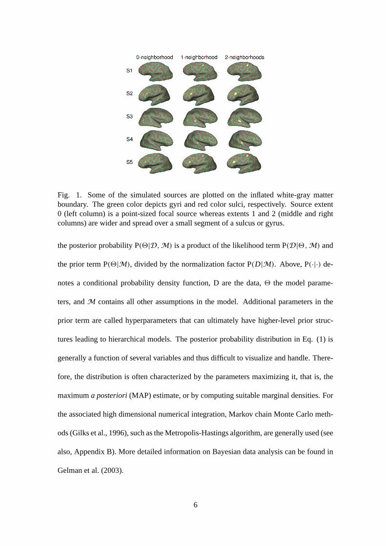
Fig. 1. Some of the simulated sources are plotted on the inflated white-gray matterboundary. The green color depicts gyri and red color sulci, respectively. Source extent0 (left column) is a point-sized focal source whereas extents 1 and 2 (middle and rightcolumns) are wider and spread over a small segment of a sulcus or gyrus.
the posterior probability P(2|D,M) is a product of the likelihood term P(D|2,M) and
the prior term P(2|M), divided by the normalization factor P(D|M). Above, P(·|·) de-
notes a conditional probability density function, D are the data, 2 the model parame-
ters, and M contains all other assumptions in the model. Additional parameters in the
prior term are called hyperparameters that can ultimately have higher-level prior struc-
tures leading to hierarchical models. The posterior probability distribution in Eq. (1) is
generally a function of several variables and thus difficult to visualize and handle. There-
fore, the distribution is often characterized by the parameters maximizing it, that is, the
maximum a posteriori (MAP) estimate, or by computing suitable marginal densities. For
the associated high dimensional numerical integration, Markov chain Monte Carlo meth-
ods (Gilks et al., 1996), such as the Metropolis-Hastings algorithm, are generally used (see
also, Appendix B). More detailed information on Bayesian data analysis can be found in
Gelman et al. (2003).
6
Source space
The white-gray matter boundary of cortex was reconstructed from 3-D T1-weighted high-
resolution MR images (MPRAGE sequence, Siemens Sonata 1.5 T, Erlangen, Germany)
using the Freesurfer software (see Fischl et al., 1999; Dale et al., 1999), with ∼150000
grid points representing each hemisphere. The resulting cortical surface geometry was
overlaid over T1-weighted images for visual verification followed by transformation into
MATLAB-environment, where the simulations and MCMC sampling were carried out.
To parametrically optimize the size of discretization of the source space, given the as-
sumption of statistical independence between neighboring source locations, the number
of possible source space points was reduced to ∼200, ∼400, ∼800, ∼1600, and ∼3200
grid points per hemisphere. Given the widely accepted assumption that cortical currents
visible to MEG are generated by synchronous post-synaptic potentials of cortical pyra-
midal neurons (Okada et al., 1997; Dale and Sereno, 1993), the orientation of the current
sources were further constrained to be perpendicular to the local surface geometry when
calculating the forward solution.
Forward model
In MEG, the Maxwell’s equations can be solved under the quasistatic approximation as-
sumption (Hämäläinen et al., 1993). The solution of the forward problem gives, for one
timepoint, the linear relationship between the source currents and the measured signals
b = As+ n, (2)
7
where b is an M×1 vector for measurements, s is an N×1 vector for the source currents, A
is an M×N gain matrix, and n a Gaussian noise vector. N is the size of the discretization
of the source space, and M is the number of measurement sensors. Each column of
A gives the measured signal distribution for one dipolar current source, located on the
cortical mantle and perpendicular to the cortical surface.
For the computation of A we employed the single-layer boundary-element model
(BEM), which assumes that the realistically-shaped cranial volume has a uniform elec-
trical conductivity and the skull is a perfect insulator. For many practical purposes this
model is sufficient in MEG source estimation (see, e.g., Hämäläinen and Sarvas, 1989;
Mosher et al., 1999).
For the locations of the sensors we utilized actual data from a measurement on the
subject whose MR images were employed in the simulation. The sensor array of the
Vectorview system used (Elekta Neuromag Oy, Helsinki, Finland) is composed of 306
sensors arranged in triplets of two planar gradiometers and a magnetometer at 102 loca-
tions. The approximate distance between adjacent sensor elements in the array is 35 mm
and the minimum distance of the sensor from the scalp is 17 mm.
The inverse problem
Biomagnetic inverse problem (Sarvas, 1987) stands for solving the underlying currents in
the living brain given the MEG measurements. Mathematically, the problem involves esti-
mating s in Eq. (2) from samples of b. In this estimation task, the gain matrix A is usually
assumed to be precisely known. In our model, the number of measurements M = 306
is much smaller than the number of points in the used grids and, therefore, the problem
is underdetermined and does not have a unique solution. Furthermore, neighboring sen-
8
sors have overlapping, non-orthogonal sensitivity patterns (lead fields; Hämäläinen et al.,
1993) and, as a result, the number of independent equations is even less than M .
The `p-norm model
We present a Bayesian model consisting of a Gaussian likelihood for the measurements
and `p-norm prior for the source current parameters. In statistical terms, Eq. (2) can be
written as a linear regression model. Assuming statistically independent measurements
b = [b1, b2, . . . , bM ] and zero-mean M-dimensional normal distribution for the noise,
given source current parameters s, the likelihood is
P(b|s,C) = 1√
det C√
2πM· exp
(− 1
2(b− As)TC−1(b− As)
), (3)
where C is the noise covariance matrix for the measurements. In this study, C is assumed
to be known up to an unknown scaling factor of σl , so that C = σ 2l C where C is known
and diagonal. For computational convenience we introduce whitening of the gain matrix,
A, and measurements, b, with the known part of the noise covariance matrix, so that
A = C−1/2A and (4)
b = C−1/2b. (5)
Leaving out numerical constants, the likelihood simplifies to
P(b|s, σl) ∝ 1
σ Ml
· exp(− 1
2σ 2l
(b− As
)T(b− As)). (6)
9
The scaling factor σl in the exponent function is a parameter for compensating unknown
alternations in the noise level. For simplification, σl was assumed having a uniform prior
instead of a more conventional choice of 1/σl , which would lead to uniform prior for
log(σl). When M is large and σl close to one, then 1/σ Ml ≈ 1/σM+1
l , and the choice of
uniform prior for σl is justifiable. In the simulation part of this study, the sampling of the
posterior distribution of σl is likely to yield values around one as the whitening was done
with a known (simulated) noise covariance matrix. In the case of real data, C is estimated
from the measurement data and σl would contain, for instance, information on uncertainty
of the whitening.
The `p-norm for vector v is
‖v‖p =(∑
i
|vi |p)1/p
. (7)
In order to reduce the correlations between the formal ` p-norm prior width and the source
current parameters (evident in our preliminary sampling runs), yet maintaining a contin-
uous variable of the norm order p for our prior, we reparametrize its structure. First,
consider a standardized normal distribution
P(x) = k · exp(− 1
2|x |q
)with q = 2. (8)
If we let q take any values other than 2 the class of exponential power distributions is
obtained. According to Box and Tiao (1973, Ch. 3.2.1); with q = 2/(1 + β) these
10
distributions can be written as
P(y|θ, φ, β) = ω(β)φ−1exp
(− c(β)
∣∣∣ y − θφ
∣∣∣2/(1+β))
, −∞ < y <∞, (9)
where
c(β) =[0(3
2(1+ β))
0(1
2(1+ β))]1/(1+β)
, −∞ < θ <∞, (10)
ω(β) = 0(3
2(1+ β))1/2
(1+ β)0(12(1+ β)
)3/2 , φ > 0, and − 1 < β ≤ 1. (11)
Parameters θ and φ are the mean and standard deviation of the population, respectively.
In our model, Eq. (9) is written as
P(si |σc, β) = ω(β)σ−1c exp
(− c(β)
∣∣∣ si
σc
∣∣∣2/(1+β)) ∀i = 1 . . . N , (12)
in which the elements of vector s = [s1, s2, . . . , sN ] are assumed independent, θ = 0, and
c(β) and ω(β) are as above. β is a hyperparameter parametrizing the ` p-norm order p
and σc is the variance of the source current amplitudes (prior width). In the Bayesian a
priori distribution, this variance corresponds to regularization of the inverse solution and
in that sense it could also be called a regularization parameter. Further on, the joint prior
for the source currents is simply the product of all the independent elements
P(s|σc, β) = ω(β)Nσ−Nc exp
(− c(β)
∑
i
∣∣∣ si
σc
∣∣∣2/(1+β))
. (13)
The energy function corresponding to the prior is defined as a negative natural logarithm
11
of Eq. (13)
−lnP(s|σc, β) = −N ln
(ω(β)
σc
)+ c(β)
∑
i
(∣∣∣ si
σc
∣∣∣2/(1+β))
. (14)
By substituting β = 0 and β = 1 to the sum expression of Eq. (14), it simplifies to
∑
i
∣∣∣ si
σc
∣∣∣2 = 1
σ 2c
∑
i
|si |2 = 1
σ 2c‖s‖ 2
2 and (15)
∑
i
∣∣∣ si
σc
∣∣∣1 = 1
σc
∑
i
|si |1 = 1
σc‖s‖ 1
1 , respectively. (16)
Thus, our model imposes the `p-norm (see Eq. (7)) prior for the currents so that, when
β = 1, the model corresponds to `1-norm, and when β = 0, the model imposes the
Euclidean norm, or `2-norm prior, for the source currents. Values 0 < β < 1 correspond
to values of p between 2 and 1, respectively. Similarly to σl in Eq. (6), a uniform prior
was also assumed for both hyperparameters σc and β. Notice, that β is a hyperparameter
defining the `p-norm order, so that
p = 2
1+ β. (17)
Consequently, our choice of uniform prior for β will have an effect on the implicit prior
of p, so that the model slightly favors values of p close to 1 over the values of p close to
2. In Bayesian data analysis, this effect might be transferred to the shape of the posterior
distribution of p and could be relevant in making inferences based on the analysis. With
the presented `p-norm model this effect was insignificant considering our conclusions.
To show this, we performed a prior sensitivity analysis for β, which is described in more
12
detailed fashion in Appendix A.
Collecting the pieces of our `p-norm model according to Bayes’ rule in Eq. (1) and
leaving out the normalization factor which is not required for numerical considerations,
the joint posterior probability distribution for the source currents s, parameter σl , and
model hyperparameters σc and β
P(s, σl, σc, β|b) ∝ P(b|s, σl) · P(σl) · P(s|σc, β) · P(σc) · P(β), (18)
where model assumptions are explicitly defined in the text, hyperpriors P(σl), P(σc), and
P(β) are assumed uniform, and P(b|s, σl) and P(s|σc, β) are as in Eqs. (6) and (13),
respectively. In the results and discussion sections of the paper we present the posterior
distributions of p according to Eq. (17) and utilize only the parameter p to facilitate the
reading.
Simulated data sets
We utilized four functionally relevant source locations in data simulations: the left mo-
tor cortex (S1), left dorsolateral prefrontal cortex (S2), right posterior superior temporal
sulcus (S3), and right primary auditory cortex (S4). With each location, at least three
source extents were used. The first source extent contained only a single active source
space point (0-neighborhood). The other types contained 1- and 2-neighborhoods of the
one center point along the original source space grid. On average, these correspond to
point-sized, ∼0.2 cm2, and ∼0.7 cm2 physical sizes on the white-gray matter boundary.
In this paper, the source extent is denoted with subindex (e.g., S10). The anatomical loca-
tions and sources are shown on the inflated white-gray matter boundary in Fig. 1. Mainly
13
we simulated single sources, but also combinations of sources were studied so that the
total number of different source configurations that were used to determine the optimal
grid discretization size was 21. To investigate the effect of the extent of the underlying
source configuration, two sources (S1 and S4) were additionally analyzed with 4- and
8-neighborhoods (∼3 cm2 and ∼15 cm2, respectively). The source current amplitude
was set to be 80 nAm for the whole source regardless of its extent. For the combinatory
sources S5 (S1 and S2 active together), the source current amplitudes were 80 nAm for
both or alternatively 80 nAm for one and 40 nAm for the other.
Data were generated by using the forward model in Eq. (2) to create the fields for one
timepoint. Maximum amplitudes of the resulting magnetic fields and magnetic field gra-
dients were realistic, approximately 200–400 fT for magnetometers and 50–200 fT/cm for
gradiometers. The gain matrix A used in the forward computation included 306 rows and
approximately 32000 columns. This way, the original source space grid size contained
∼16000 points per hemisphere and consequently, as the solution grid sizes were all sig-
nificantly smaller, the most obvious type of inverse crime was avoided. The term inverse
crime is used to describe all those elements that are fixed in the data generating model
and later presumed known in the solution part. Naturally, in simulation studies such mod-
elling flaws might lead to improved and too optimistic results, but also to overfitting and
spurious models which would likely fail in real data scenarios.
Random zero-mean Gaussian noise was added to the simulated measurement vector
b, so that the mean signal-to-noise ratio described by
SNR = bTbMσ 2
n(19)
14
was 15 for magnetometers and about 60 for gradiometers. M is the number of sensors and
σn is the standard deviation of the corresponding sensor noise. The measurement noise
was assumed equal separately within the three sets of different sensors (i.e., two sets of
gradiometers, one set of magnetometers). In most cases, SNR was set to be rather good,
because we were mainly interested whether there is information in the data to determine
the norm order p. The effect of SNR to the model was examined with two sources S12
and S41, so that the mean SNR for gradiometer measurements was approximately 5, 15,
30, 60, and 90 (1.25, 3.75, 7.5, 15, and 22.5 for magnetometers). After adding the noise,
the simulated data were whitened according to Eq. (5).
Real MEG data
The real MEG data set contained evoked fields of a self-paced index finger lifting ex-
periment of a one right-handed male, aged 27. There were two conditions: the subject
lifted his (A) right and (B) left index finger. Electro-oculogram (EOG) artefact rejection
threshold (peak-to-peak) was set to 150 µV, so that 111 accepted trials were averaged in
the first condition and 113 in the second one. The measured data vector b was taken at
a latency of 20 ms from the onset of finger movement in both conditions. The known
part of the noise covariance matrix C (see Eq. (5)) was estimated as a variance of each
sensor from a 2-minute fragment of filtered mesurement data acquired when the subject
was sitting in the shielded room under the MEG device doing nothing prior to the actual
experiment. To reflect the decrease of noise due to averaging, C was scaled by dividing
it by the number of trials averaged separately for both conditions. A Hamming window
based digital filter was used to remove noise from the averaged evoked fields and the frag-
ment of data from which C was estimated. The passband edge frequencies were [2 18]
15
Hz and stopband edge frequencies [0.5 20] Hz. The estimated mean signal-to-noise ratio
for the utilized data was approximately 6/0.1 for condition A gradiometer/magnetometer
measurements and 8/0.1 for condition B. However, the sensors that mostly contained the
signal (i.e., the best SNR), had a fairly good SNR of about 40–70 for gradiometers and
1–2 for magnetometers.
Sampling procedure and inverse estimation
All parameters of the model, including source currents s, hyperparameter β, likelihood
standard deviation σl , and prior width σc, were considered as random variables and their
distributions were obtained utilizing an MCMC method called slice sampling. Samples
were drawn from the joint posterior distribution of the currents and model parameters (Eq.
(18)) using modern Linux-workstations (Pentium III/4, 1–3.2 GHz processor, 1024–4096
MB of RAM). Slice sampling is often more efficient than simple Metropolis updates as
it adaptively chooses the magnitude of the changes made. Convergence diagnostics and
time series analysis, such as potential scale reduction factor (PSRF), were used to verify
that the convergence of the sampler was plausible (Robert and Casella, 2004). For more
information on utilized sampling method and convergence diagnostics see Appendix B.
The inverse estimates were calculated as posterior expectation values of the currents
integrated over the hyperparameters β, σc, and σl . This was done for all the simulated
sources using the `p-norm prior model. For visualization purposes the estimates on each
grid size were thresholded by setting to zero the current amplitude of all the source points
whose absolute amplitude value did not exceed 20% of the peak value of that particular
estimate. In most cases, the solution estimates were also interpolated on the original
cortical mantle (∼16000), so that the visual comparison with the simulated sources would
16
be easier.
Model choice
In addition to the visual examination of the quality of the solutions, the model good-
ness was estimated with a method based on posterior predictive sampling. Gelfand and
Ghosh (1998) propose a minimum posterior predictive loss approach in which the cri-
terion, whose minimum defines the optimal model, comprises of a goodness-of-fit term
Gm and a penalty term Pm , where m denotes the model. In our study, the term Gm was
calculated as a sum of squared error of the model predicted measurements averaged over
21 different sources that were used in the analysis, and Pm was determined by the sum
of predictive variances of the measurements. The predictive distribution of the measure-
ments was attained by computing it using the forward model in Eq. (2) with the source
current samples. In this particular case, the posterior predictive sampling is easy to do as
we already have a large amount of Monte Carlo samples obtained from the posterior dis-
tribution. The minimum posterior predictive loss criterion for model m, Dm = Gm + Pm
(Gelfand and Ghosh, 1998), was calculated as an average over all the sources analyzed
in this study, and thus considering the grid size as a variable altering the model struc-
ture. Furthermore, our `p-norm model was compared with similar `1- and `2-norm prior
models by analyzing simulated data sets shown in Fig. 1. These models were realized as
special cases of the `p-norm model by setting the hyperparameter β to 1 and 0, respec-
tively. Based on the obtained posterior distributions, we also performed model choice
using the minimum posterior predictive loss approach.
17
Results
An MCMC chain was produced for each of the simulated sources and for each of the
grid sizes separately. For the smaller grid sizes (∼200, ∼400, and ∼800 points per hemi-
sphere) the time required to draw one sample (i.e., one set of source current parameters
and hyperparameters) from the joint posterior distribution was in the order of 1–4 sec-
onds. At least 10000 samples were drawn for each of these chains. For the chains of the
larger grid sizes (∼1600 and∼3200 per hemisphere) the time required for one sample was
about 10–25 seconds. Despite the time-consuming computer runs, at least 3000 samples
were drawn for these chains.
The convergence of the sampler appeared to be plausible by the potential scale reduc-
tion factor (see Appendix B.2.), which was estimated either for the different segments of
one chain or from several chains of the same source with different initial conditions. The
chains seemed to converge also based on visual inspection of the obtained samples. Time
series analysis revealed that autocorrelation times of the samples were in general quite
long. For some source current parameters and hyperparameters, the autocorrelation time
was in the order of several hundreds or even over one thousand samples. This means,
that from a chain of 10000 samples we get effectively only ∼50 independent samples or
even less. Inverse estimates were obtained from these independent samples by implic-
itly integrating the posterior of source current parameters over the hyperparameters and
computing the expectation value for s. Low number of independent samples increases the
Monte Carlo error of this estimate, but 10–50 is enough for a reasonable one.
Inverse estimates for simulated sources S10, S21, and S41 are shown with the original
sources in Fig. 2. The utilized grid sizes for sampling these inverse estimates were ∼800
18
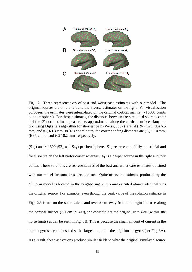
Fig. 2. Three representatives of best and worst case estimates with our model. Theoriginal sources are on the left and the inverse estimates on the right. For visualizationpurposes, the estimates were interpolated on the original cortical mantle (∼16000 pointsper hemisphere). For these estimates, the distances between the simulated source centerand the `p-norm estimate peak value, approximated along the cortical surface triangula-tion using Dijkstra’s algorithm for shortest path (Weiss, 1997), are (A) 26.7 mm, (B) 6.5mm, and (C) 69.3 mm. In 3-D coordinates, the corresponding distances are (A) 11.0 mm,(B) 5.2 mm, and (C) 18.2 mm, respectively.
(S10) and ∼1600 (S21 and S41) per hemisphere. S10 represents a fairly superficial and
focal source on the left motor cortex whereas S41 is a deeper source in the right auditory
cortex. These solutions are representatives of the best and worst case estimates obtained
with our model for smaller source extents. Quite often, the estimate produced by the
`p-norm model is located in the neighboring sulcus and oriented almost identically as
the original source. For example, even though the peak value of the solution estimate in
Fig. 2A is not on the same sulcus and over 2 cm away from the original source along
the cortical surface (∼1 cm in 3-D), the estimate fits the original data well (within the
noise limits) as can be seen in Fig. 3B. This is because the small amount of current in the
correct gyrus is compensated with a larger amount in the neighboring gyrus (see Fig. 3A).
As a result, these activations produce similar fields to what the original simulated source
19
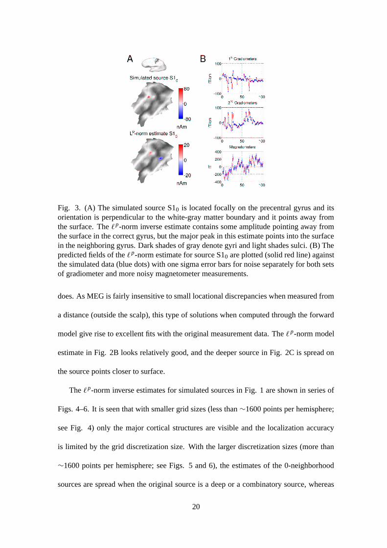
Fig. 3. (A) The simulated source S10 is located focally on the precentral gyrus and itsorientation is perpendicular to the white-gray matter boundary and it points away fromthe surface. The `p-norm inverse estimate contains some amplitude pointing away fromthe surface in the correct gyrus, but the major peak in this estimate points into the surfacein the neighboring gyrus. Dark shades of gray denote gyri and light shades sulci. (B) Thepredicted fields of the `p-norm estimate for source S10 are plotted (solid red line) againstthe simulated data (blue dots) with one sigma error bars for noise separately for both setsof gradiometer and more noisy magnetometer measurements.
does. As MEG is fairly insensitive to small locational discrepancies when measured from
a distance (outside the scalp), this type of solutions when computed through the forward
model give rise to excellent fits with the original measurement data. The ` p-norm model
estimate in Fig. 2B looks relatively good, and the deeper source in Fig. 2C is spread on
the source points closer to surface.
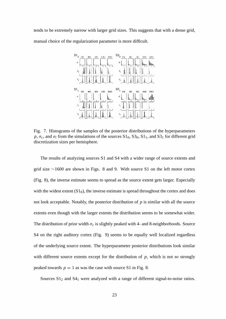
The `p-norm inverse estimates for simulated sources in Fig. 1 are shown in series of
Figs. 4–6. It is seen that with smaller grid sizes (less than ∼1600 points per hemisphere;
see Fig. 4) only the major cortical structures are visible and the localization accuracy
is limited by the grid discretization size. With the larger discretization sizes (more than
∼1600 points per hemisphere; see Figs. 5 and 6), the estimates of the 0-neighborhood
sources are spread when the original source is a deep or a combinatory source, whereas
20
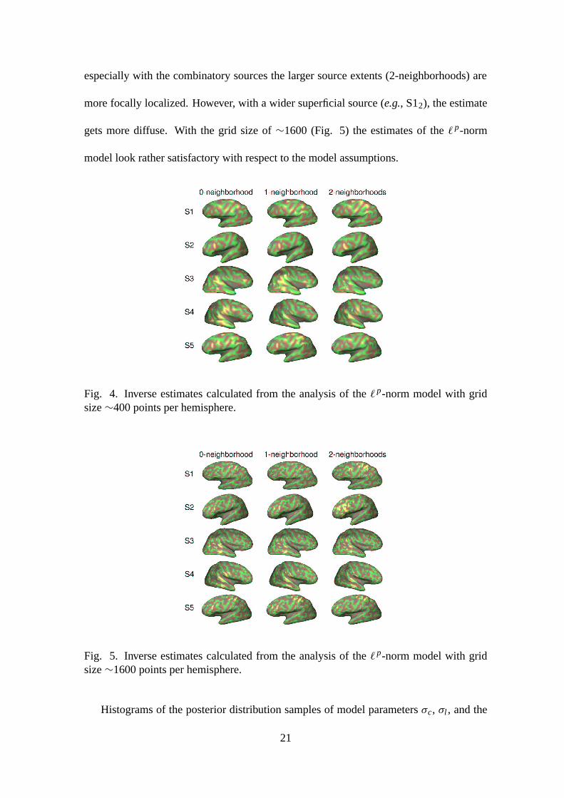
especially with the combinatory sources the larger source extents (2-neighborhoods) are
more focally localized. However, with a wider superficial source (e.g., S12), the estimate
gets more diffuse. With the grid size of ∼1600 (Fig. 5) the estimates of the ` p-norm
model look rather satisfactory with respect to the model assumptions.
Fig. 4. Inverse estimates calculated from the analysis of the ` p-norm model with gridsize ∼400 points per hemisphere.
Fig. 5. Inverse estimates calculated from the analysis of the ` p-norm model with gridsize ∼1600 points per hemisphere.
Histograms of the posterior distribution samples of model parameters σc, σl , and the
21
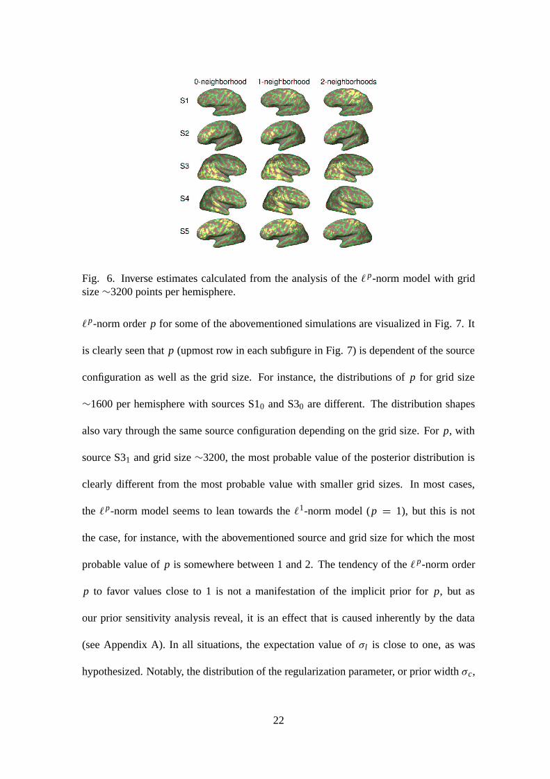
Fig. 6. Inverse estimates calculated from the analysis of the ` p-norm model with gridsize ∼3200 points per hemisphere.
`p-norm order p for some of the abovementioned simulations are visualized in Fig. 7. It
is clearly seen that p (upmost row in each subfigure in Fig. 7) is dependent of the source
configuration as well as the grid size. For instance, the distributions of p for grid size
∼1600 per hemisphere with sources S10 and S30 are different. The distribution shapes
also vary through the same source configuration depending on the grid size. For p, with
source S31 and grid size ∼3200, the most probable value of the posterior distribution is
clearly different from the most probable value with smaller grid sizes. In most cases,
the `p-norm model seems to lean towards the `1-norm model (p = 1), but this is not
the case, for instance, with the abovementioned source and grid size for which the most
probable value of p is somewhere between 1 and 2. The tendency of the ` p-norm order
p to favor values close to 1 is not a manifestation of the implicit prior for p, but as
our prior sensitivity analysis reveal, it is an effect that is caused inherently by the data
(see Appendix A). In all situations, the expectation value of σl is close to one, as was
hypothesized. Notably, the distribution of the regularization parameter, or prior width σc,
22
tends to be extremely narrow with larger grid sizes. This suggests that with a dense grid,
manual choice of the regularization parameter is more difficult.
Fig. 7. Histograms of the samples of the posterior distributions of the hyperparametersp, σc, and σl from the simulations of the sources S10, S30, S11, and S31 for different griddiscretization sizes per hemisphere.
The results of analyzing sources S1 and S4 with a wider range of source extents and
grid size ∼1600 are shown in Figs. 8 and 9. With source S1 on the left motor cortex
(Fig. 8), the inverse estimate seems to spread as the source extent gets larger. Especially
with the widest extent (S18), the inverse estimate is spread throughout the cortex and does
not look acceptable. Notably, the posterior distribution of p is similar with all the source
extents even though with the larger extents the distribution seems to be somewhat wider.
The distribution of prior width σc is slightly peaked with 4- and 8-neighborhoods. Source
S4 on the right auditory cortex (Fig. 9) seems to be equally well localized regardless
of the underlying source extent. The hyperparameter posterior distributions look similar
with different source extents except for the distribution of p, which is not so strongly
peaked towards p = 1 as was the case with source S1 in Fig. 8.
Sources S12 and S41 were analyzed with a range of different signal-to-noise ratios.
23
Fig. 8. The simulated source S1 with 0-, 1-, 2-, 4-, and 8-neighborhoods is plottedon the white-gray matter boundary on the top row. The ` p-norm estimates with griddiscretization size ∼1600 are shown on the second row. For the corresponding estimates,the posterior distributions of the model parameters p, σc, and σl are shown below.
The corresponding inverse estimates are shown in Fig. 10 and labeled with gradiome-
ter mean SNR, respectively. The utilized grid size was ∼1600 per hemisphere. Original
simulated sources of these estimates can be seen in Figs. 1 and 2. With all the utilized
SNR values, the inverse estimates of superficial source S12 and deep source S41 are sim-
ilar with each other. With SNR=5, especially the inverse estimate of source S41 is more
spread along the cortex. In Fig. 11 one can see the hyperparameter posterior distributions
of the samples of these particular estimates. Even though the distributions of the ` p-norm
order p are more diffuse with poorer SNR, suggesting that the determination of p be-
comes more difficult with more noise, it seems clear that the model favors values close
to 1 in these cases. Importantly, by examining the distribution of parameter p it can be
seen that the most probable value of p for source S41 and SNR=5 might be where the
distribution has the most mass (i.e., between 1 and 1.5), even though the maximum of this
distribution appears to be at 1. This effect is most likely due to high noise, but in some
cases the posterior distribution might indeed be multimodal.
24
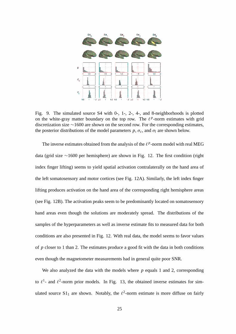
Fig. 9. The simulated source S4 with 0-, 1-, 2-, 4-, and 8-neighborhoods is plottedon the white-gray matter boundary on the top row. The ` p-norm estimates with griddiscretization size ∼1600 are shown on the second row. For the corresponding estimates,the posterior distributions of the model parameters p, σc, and σl are shown below.
The inverse estimates obtained from the analysis of the ` p-norm model with real MEG
data (grid size ∼1600 per hemisphere) are shown in Fig. 12. The first condition (right
index finger lifting) seems to yield spatial activation contralaterally on the hand area of
the left somatosensory and motor cortices (see Fig. 12A). Similarly, the left index finger
lifting produces activation on the hand area of the corresponding right hemisphere areas
(see Fig. 12B). The activation peaks seem to be predominantly located on somatosensory
hand areas even though the solutions are moderately spread. The distributions of the
samples of the hyperparameters as well as inverse estimate fits to measured data for both
conditions are also presented in Fig. 12. With real data, the model seems to favor values
of p closer to 1 than 2. The estimates produce a good fit with the data in both conditions
even though the magnetometer measurements had in general quite poor SNR.
We also analyzed the data with the models where p equals 1 and 2, corresponding
to `1- and `2-norm prior models. In Fig. 13, the obtained inverse estimates for sim-
ulated source S11 are shown. Notably, the `2-norm estimate is more diffuse on fairly
25
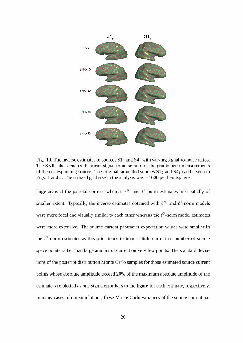
Fig. 10. The inverse estimates of sources S12 and S41 with varying signal-to-noise ratios.The SNR label denotes the mean signal-to-noise ratio of the gradiometer measurementsof the corresponding source. The original simulated sources S12 and S41 can be seen inFigs. 1 and 2. The utilized grid size in the analysis was ∼1600 per hemisphere.
large areas at the parietal cortices whereas `p- and `1-norm estimates are spatially of
smaller extent. Typically, the inverse estimates obtained with ` p- and `1-norm models
were more focal and visually similar to each other whereas the `2-norm model estimates
were more extensive. The source current parameter expectation values were smaller in
the `2-norm estimates as this prior tends to impose little current on number of source
space points rather than large amount of current on very few points. The standard devia-
tions of the posterior distribution Monte Carlo samples for those estimated source current
points whose absolute amplitude exceed 20% of the maximum absolute amplitude of the
estimate, are plotted as one sigma error bars to the figure for each estimate, respectively.
In many cases of our simulations, these Monte Carlo variances of the source current pa-
26
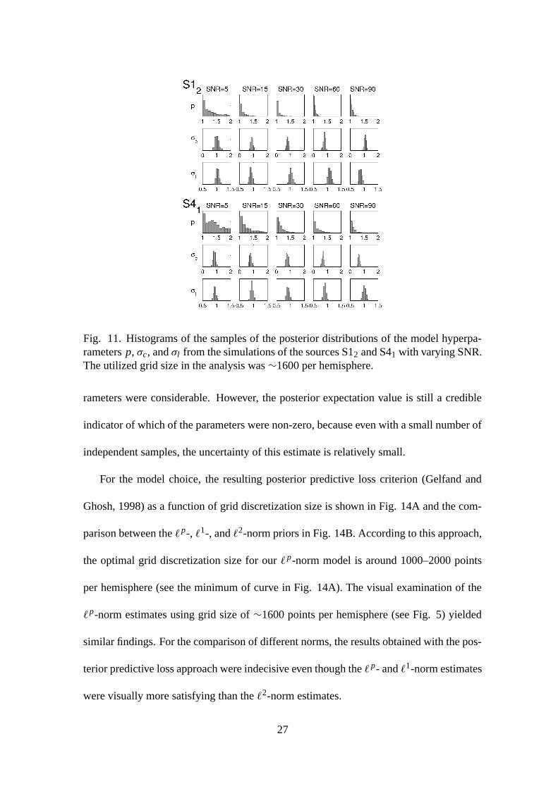
Fig. 11. Histograms of the samples of the posterior distributions of the model hyperpa-rameters p, σc, and σl from the simulations of the sources S12 and S41 with varying SNR.The utilized grid size in the analysis was ∼1600 per hemisphere.
rameters were considerable. However, the posterior expectation value is still a credible
indicator of which of the parameters were non-zero, because even with a small number of
independent samples, the uncertainty of this estimate is relatively small.
For the model choice, the resulting posterior predictive loss criterion (Gelfand and
Ghosh, 1998) as a function of grid discretization size is shown in Fig. 14A and the com-
parison between the `p-, `1-, and `2-norm priors in Fig. 14B. According to this approach,
the optimal grid discretization size for our `p-norm model is around 1000–2000 points
per hemisphere (see the minimum of curve in Fig. 14A). The visual examination of the
`p-norm estimates using grid size of ∼1600 points per hemisphere (see Fig. 5) yielded
similar findings. For the comparison of different norms, the results obtained with the pos-
terior predictive loss approach were indecisive even though the ` p- and `1-norm estimates
were visually more satisfying than the `2-norm estimates.
27
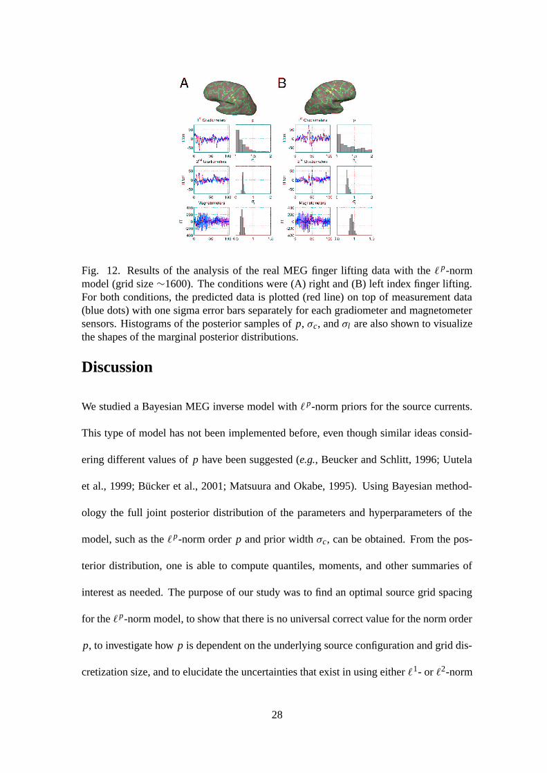
Fig. 12. Results of the analysis of the real MEG finger lifting data with the ` p-normmodel (grid size ∼1600). The conditions were (A) right and (B) left index finger lifting.For both conditions, the predicted data is plotted (red line) on top of measurement data(blue dots) with one sigma error bars separately for each gradiometer and magnetometersensors. Histograms of the posterior samples of p, σc, and σl are also shown to visualizethe shapes of the marginal posterior distributions.
Discussion
We studied a Bayesian MEG inverse model with `p-norm priors for the source currents.
This type of model has not been implemented before, even though similar ideas consid-
ering different values of p have been suggested (e.g., Beucker and Schlitt, 1996; Uutela
et al., 1999; Bücker et al., 2001; Matsuura and Okabe, 1995). Using Bayesian method-
ology the full joint posterior distribution of the parameters and hyperparameters of the
model, such as the `p-norm order p and prior width σc, can be obtained. From the pos-
terior distribution, one is able to compute quantiles, moments, and other summaries of
interest as needed. The purpose of our study was to find an optimal source grid spacing
for the `p-norm model, to show that there is no universal correct value for the norm order
p, to investigate how p is dependent on the underlying source configuration and grid dis-
cretization size, and to elucidate the uncertainties that exist in using either `1- or `2-norm
28
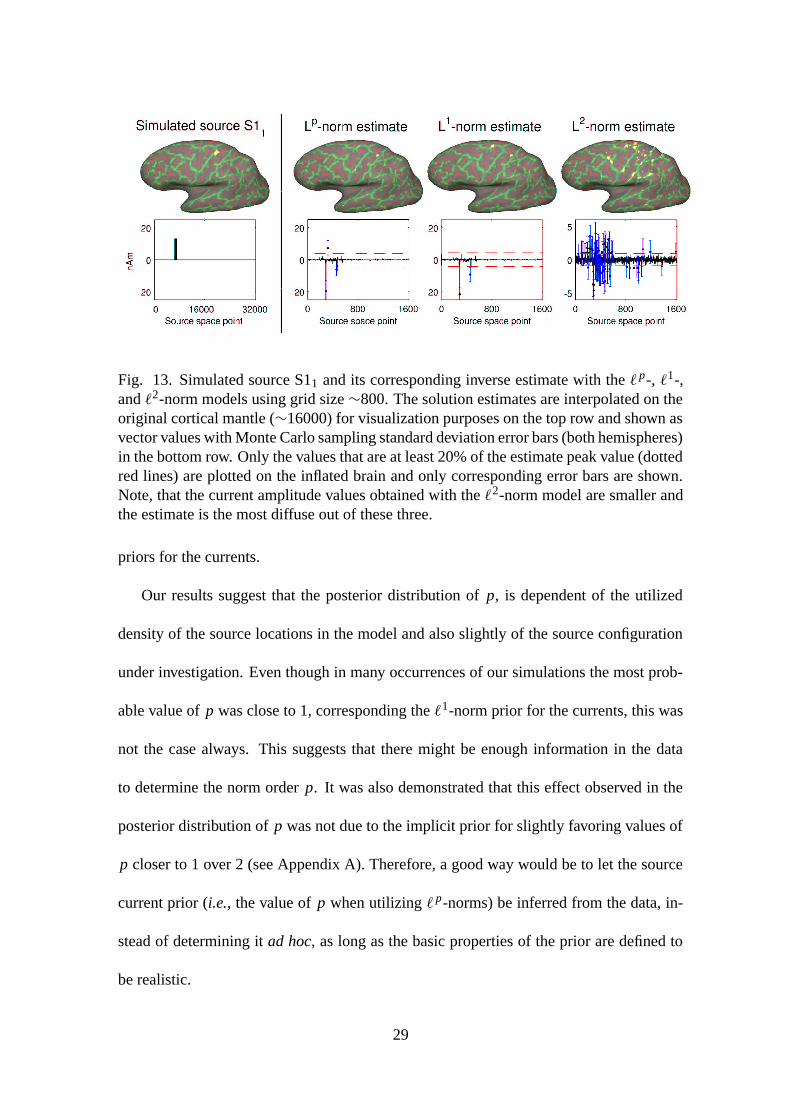
Fig. 13. Simulated source S11 and its corresponding inverse estimate with the `p-, `1-,and `2-norm models using grid size ∼800. The solution estimates are interpolated on theoriginal cortical mantle (∼16000) for visualization purposes on the top row and shown asvector values with Monte Carlo sampling standard deviation error bars (both hemispheres)in the bottom row. Only the values that are at least 20% of the estimate peak value (dottedred lines) are plotted on the inflated brain and only corresponding error bars are shown.Note, that the current amplitude values obtained with the `2-norm model are smaller andthe estimate is the most diffuse out of these three.
priors for the currents.
Our results suggest that the posterior distribution of p, is dependent of the utilized
density of the source locations in the model and also slightly of the source configuration
under investigation. Even though in many occurrences of our simulations the most prob-
able value of p was close to 1, corresponding the `1-norm prior for the currents, this was
not the case always. This suggests that there might be enough information in the data
to determine the norm order p. It was also demonstrated that this effect observed in the
posterior distribution of p was not due to the implicit prior for slightly favoring values of
p closer to 1 over 2 (see Appendix A). Therefore, a good way would be to let the source
current prior (i.e., the value of p when utilizing ` p-norms) be inferred from the data, in-
stead of determining it ad hoc, as long as the basic properties of the prior are defined to
be realistic.
29
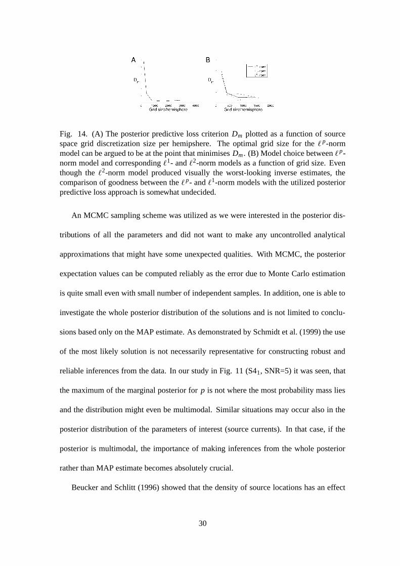
Fig. 14. (A) The posterior predictive loss criterion Dm plotted as a function of sourcespace grid discretization size per hemipshere. The optimal grid size for the ` p-normmodel can be argued to be at the point that minimises Dm . (B) Model choice between `p-norm model and corresponding `1- and `2-norm models as a function of grid size. Eventhough the `2-norm model produced visually the worst-looking inverse estimates, thecomparison of goodness between the `p- and `1-norm models with the utilized posteriorpredictive loss approach is somewhat undecided.
An MCMC sampling scheme was utilized as we were interested in the posterior dis-
tributions of all the parameters and did not want to make any uncontrolled analytical
approximations that might have some unexpected qualities. With MCMC, the posterior
expectation values can be computed reliably as the error due to Monte Carlo estimation
is quite small even with small number of independent samples. In addition, one is able to
investigate the whole posterior distribution of the solutions and is not limited to conclu-
sions based only on the MAP estimate. As demonstrated by Schmidt et al. (1999) the use
of the most likely solution is not necessarily representative for constructing robust and
reliable inferences from the data. In our study in Fig. 11 (S41, SNR=5) it was seen, that
the maximum of the marginal posterior for p is not where the most probability mass lies
and the distribution might even be multimodal. Similar situations may occur also in the
posterior distribution of the parameters of interest (source currents). In that case, if the
posterior is multimodal, the importance of making inferences from the whole posterior
rather than MAP estimate becomes absolutely crucial.
Beucker and Schlitt (1996) showed that the density of source locations has an effect
30
on the norm order p. Our results indicate that a dense discretization seems to favor values
of p closer to 2. The optimal discretization size for our model was ∼1500 points per
hemisphere. If number of sources is decreased to 200–400 points per hemisphere, the
accuracy of the estimates is not good and the model does not fit the data well, because the
grid is too sparse and only major cortical structures are visible. As the discretization size
increases, the goodness-of-fit improves, but with really dense grids the proposed ` p-norm
model becomes unacceptably heavy to compute, and at the same time the model prior
assumption of independent source currents is severely violated.
One way to ease the computational load would be to decrease the number of parame-
ters by parametrizing the sources. For example, Schmidt et al. (1999) employed regional
source model, which was characterized by three parameters comprising of number, loca-
tion, and extent of the active regions. This way, they decreased the number of parameters
sampled from several thousands to only three (per activity region). In this case, one in-
troduces some spatial dependency to the model as the points inside the active regions are
assumed to correlate strongly. The assumption of uncorrelated source space points seems
justifiable in early sensory responses while in complex cognitive tasks one may expect
correlations not only between neighboring points but between remote cortical regions as
well. However, taking this into account in the inverse model is not necessarily straight-
forward due to the absense of data on the exact nature of the correlations.
A conceivable way to take into account the putative dependencies between source
space points would be to introduce spatial priors. Also, with the current ` p-norm model,
the grid discretization size cannot be increased unless spatial priors are used. As the
most feasible spatial priors are neither simple nor intuitive, there exists some unclarity of
which kind to use. Phillips et al. (2002) suggest that the combination of functional and
31
anatomical constraints might provide a way for introducing spatial priors to the model
and at the same time for reducing the dimensionality of the MEG inverse problem. With
real data scenarios one has to remember that some sources are not visible for MEG and
therefore the use of spatial priors becomes even more important if additional information
is not available from elsewhere. The implementation and testing of such justifiable spatial
priors is left for subsequent studies.
Converging evidence from other imaging modalities, such as functional magnetic res-
onance imaging (fMRI) and electroencephalography (EEG), can be introduced to the cur-
rent `p-norm model if the utilized experimental setup is suitable for collecting data with
various methods. The combination of adjacent imaging methods (Dale et al., 2000; Liu
et al., 2002), MEG with fMRI in particular (Schulz et al., 2004; Ahlfors and Simpson,
2004; Dale et al., 2000), is going to be an invaluable tool in brain research in the future.
Even if the coupling between fMRI BOLD signal and EEG/MEG response are not well
understood, clear evidence exists on how these two fundamentally different signals are
related (Logothetis et al., 2001; Kim et al., 2004). In comparison, the combined use of
MEG and EEG is relatively straightforward as both of these methods detect the neural
electric currents. Since EEG provides information about the radial currents in addition to
the tangential ones detected by MEG, it is conceivable that the combination will provide
a more comprehensive estimate of the underlying neural events.
However, as Liu et al. (2002) and Phillips et al. (1997) suggest, the combination of
EEG and MEG might not improve the results much. Also, with EEG inverse modelling,
there exists the problem of creating a realistic forward model for EEG as in that case the
electric conductivites of the scalp, the skull, and the brain tissue and the shapes of the
corresponding compartments need to be known more precisely (Ollikainen et al., 1999).
32
In contrast, an a priori bias towards fMRI information is straightforward to add to the
current model per se. In addition, depth normalization can be included to reduce the
location bias of the estimates (Köhler et al., 1996) and, with the cost of computational
burden, the use of temporal dynamics in the model might prove to be useful especially for
empirical investigations.
Our preliminary analysis with real MEG data were promising. The results are in line
with similar MEG studies in the field (see, e.g. Alary et al., 2002). However, the appli-
cation of the model with more complex real data (e.g., cognitive tasks and audiovisual
studies) still requires work and implementation of some of the abovementioned methods
such as spatial priors and temporal dynamics. As of now, the ` p-norm model is a spatial
only MEG source localization method.
The quality of MEG inverse estimates in general is not trivial to evaluate even though
in simulation studies the original sources are known. In addition to the visual quality
of the solution estimates one can, for example, easily approximate the physical distance
between the solution peaks and original sources both along the cortical surface and in
3-D, and use this as a quantitative error. But the question arises how to penalize false
activations, for instance, in situations where the solutions are spread over the cortex, and
how to penalize the goodness of the solution if the estimate is located in the wrong gyrus
yet being highly probable (see Fig. 3). In the analysis of real data, particularly, when the
original sources are not known, different methods are needed. One way is to look at all the
solutions and compare different models with each other instead of single estimates and
their accuracy. One such method is the posterior predictive loss approach (Gelfand and
Ghosh, 1998), which we used, along with visual examination, to determine the optimal
discretization of the source space for our `p-norm model.
33
On top of being able to evaluate the whole posterior distribution of the parameters and
hyperparameters, which conceal information of the model behavior and inverse estimates,
a substantial benefit of our model is that it is very simple and therefore additional (prior)
information is easy to attach. Virtually no user expertise is required after the model is
compiled and the method can be used almost without any manual interaction or tuning,
which is not the case with ECD fitting. This feature is more or less fundamental with
many Bayesian models. Naturally, an experienced user can achieve excellent results with
methods that require more interaction, but a problem rises if one’s goal is to study cog-
nitive processes about which very little is known in advance. In those cases a model that
does not require tuning would be most convenient to use. The estimates obtained with our
`p-norm model can also be used as a starting points or seeds for other source localization
methods. This is practical when little is known of the sources under investigation.
In conclusion, the `p-norm prior family seems usable in a Bayesian setting, in which
all the parameters and hyperparameters of the model, such as the ` p-norm order p, are
considered random variables and inferred from the data. For example, the grid discretiza-
tion size and underlying source configurations have an effect on the probabilities of the
hyperparameters, and thus on choice of model. As MEG measurements with convenient
signal-to-noise ratios might provide little extra information to which model should be
used, careful data collection and a priori model consideration becomes extremely impor-
tant. As an ultimate goal, the proposed modelling scheme can be expanded to a freely
distributable environment in which different model assumptions could be compared with
each other and further developed.
34
Acknowledgements
This research was supported in part by Academy of Finland (projects: 200521, 202871,
206368), Instrumentarium Science Foundation, Finnish Cultural Foundation, National
Institutes of Health (RO1-HD40712), The MIND Institute, and Jenny and Antti Wihuri
Foundation. Authors would like to thank anonymous reviewers for helpful remarks and
Mr. Antti Yli-Krekola for a helping hand with the preprocessing of MR-images.
Appendix A. Prior sensitivity analysis for β
When transforming probability distributions from one parametrization to another, one
needs to carefully consider what kind of effects and extra terms it has on the outcome.
Gelman et al. (2003, Ch. 1.8): Suppose that Pu(u) is the density of vector u and we
want to transform to v = f (u). If Pu is continuous, and v = f (u) is a one-to-one
transformation, then the joint density of v
Pv(v) = |J | · Pu(
f −1(v)), (20)
where |J | is the determinant of the Jacobian of the transformation u = f −1(v). The
Jacobian J is a square matrix of partial derivatives, with the entry (i, j) equal to ∂u i/∂vj .
A.1. Uniform prior for β
If we want to transform to using p with the utilized parametrization (Box and Tiao, 1973)
of our `p-norm model having uniform prior probability density for β and f (β) being Eq.
35
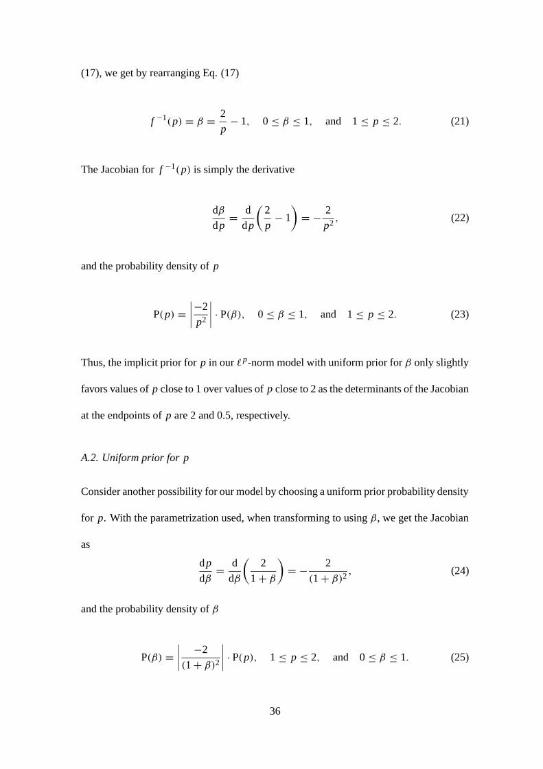
(17), we get by rearranging Eq. (17)
f −1(p) = β = 2
p− 1, 0 ≤ β ≤ 1, and 1 ≤ p ≤ 2. (21)
The Jacobian for f −1(p) is simply the derivative
dβ
dp= d
dp
(2
p− 1
)= − 2
p2, (22)
and the probability density of p
P(p) =∣∣∣∣−2
p2
∣∣∣∣ · P(β), 0 ≤ β ≤ 1, and 1 ≤ p ≤ 2. (23)
Thus, the implicit prior for p in our `p-norm model with uniform prior for β only slightly
favors values of p close to 1 over values of p close to 2 as the determinants of the Jacobian
at the endpoints of p are 2 and 0.5, respectively.
A.2. Uniform prior for p
Consider another possibility for our model by choosing a uniform prior probability density
for p. With the parametrization used, when transforming to using β, we get the Jacobian
as
dp
dβ= d
dβ
(2
1+ β)= − 2
(1+ β)2 , (24)
and the probability density of β
P(β) =∣∣∣∣−2
(1+ β)2∣∣∣∣ · P(p), 1 ≤ p ≤ 2, and 0 ≤ β ≤ 1. (25)
36
Now the implicit prior for β will slightly favor values of β close to 0 over values of β close
to 1 as the determinants of the Jacobian at the endpoints of β are 2 and 0.5, respectively.
This converts to favoring values of p close to 2 over values of p close to 1, which is
opposite to the case of uniform prior for β.
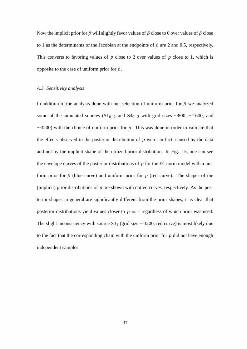
A.3. Sensitivity analysis
In addition to the analysis done with our selection of uniform prior for β we analyzed
some of the simulated sources (S10−2 and S40−2 with grid sizes ∼800, ∼1600, and
∼3200) with the choice of uniform prior for p. This was done in order to validate that
the effects observed in the posterior distribution of p were, in fact, caused by the data
and not by the implicit shape of the utilized prior distribution. In Fig. 15, one can see
the envelope curves of the posterior distributions of p for the ` p-norm model with a uni-
form prior for β (blue curve) and uniform prior for p (red curve). The shapes of the
(implicit) prior distributions of p are shown with dotted curves, respectively. As the pos-
terior shapes in general are significantly different from the prior shapes, it is clear that
posterior distributions yield values closer to p = 1 regardless of which prior was used.
The slight inconsistency with source S31 (grid size ∼3200, red curve) is most likely due
to the fact that the corresponding chain with the uniform prior for p did not have enough
independent samples.
37
Fig. 15. Blue lines denote the envelope curves of the posterior distribution shapes ofparameter p for the proposed `p-norm model with uniform prior for β (implicitly favoringvalues of p closer to 1 than 2, dotted blue line), and red lines denote the envelope curvesof the posterior distribution shapes of parameter p for the model having a uniform priorfor p (implicitly favoring values of β closer to 0 than 1, that is, in terms of p values closerto 2 than 1, dotted red curve). The posterior distribution of the norm order p is not overlysensitive to different priors and thus the observed posterior effects originate from the data.
Appendix B. Sampling method and diagnostics
B.1. Slice sampling
In Bayesian data analysis (Gelman et al., 2003), applications of Markov chain Monte
Carlo sampling often involve retrieving samples from the joint posterior distribution of
the parameters and hyperparameters of the model. In Metropolis-Hastings scheme, badly
selected scale of the proposal distribution leads to high rejection rate or inefficient random
walk. Slice sampling (Neal, 2003) relies on the principle that one can sample uniformly
under the curve of some known probability density function P(·). With slice sampling,
unlike in Gibbs sampling (Gilks et al., 1996), the conditional distributions of standard
38
form do not need to be known, and with multimodal distributions slice sampling is of-
ten more efficient than simple Metropolis-Hastings algorithm in making jumps from one
mode to another. Slice sampling adapts to the local properties of the target distribution
and it requires very little tuning. With multidimensional distributions, each variable can
be updated in turn.
A converging Markov chain towards the target distribution can be obtained by sam-
pling uniformly by turns in vertical direction under the curve and horizontally from a
slice defined by this vertical position. Let the variable to be updated be x and f (x) is the
function proportional to the probability density of x . The idea for producing a chain for
x is to replace the current value xold with a new value xnew. Draw a real value of y from
0 < y < f (xold) which defines a horizontal slice S = {x : y < f (x)}. Find an interval
I around xold that contains much or all of the slice S. Now, draw xnew uniformly from
the part of the slice within interval I and repeat the procedure. There are several different
schemes for finding the interval I that are well covered in the work by Neal (2003). In
fact, the interval can be chosen in any way as long as the resulting Markov chain remains
invariant.
For computational purposes, in order to avoid possible problems with floating-point
underflow, an energy function of f (x), g(x) = −ln( f (x)) is often calculated instead of
f (x) itself. With this particular case, a variable z = ln(y) = −g(xold) − e can be cal-
culated to define the slice S = {x : z < −g(x)}. Variable e is exponentially distributed
with mean one. Also, for our simulations, as the sampling was done one variable (source
current parameters s = [s1, s2, . . . , sN ], β, σc, and σl) at a time we optimized the perfor-
mance of the sampler by updating only the change caused by this particular variable to
the value of the energy function of the joint posterior distribution rather than computing
39
it completely every time each variable was updated.
B.2. Convergence diagnostics
There are two types of difficulties with iterative simulations such as MCMC simulations.
The simulations might not have been proceeded long enough so that the resulting samples
are not yet representative of the target distribution. The early iterations are also influenced
by the starting point rather than the target distribution. After a plausible convergence is
reached, the chain has forgot its starting point and produces representative values of the
target distribution. The early iterations are removed from the beginning of the chain.
The other problem lies in the correlation within the converging chain. In general, it
is better to start several chains with different starting points especially if the autocorrela-
tion time of the chain is long. This way, when the chains have converged, the number of
independent samples is greater than with one long chain. However, all the converged sam-
ples can still be used as the order in which they were drawn is ignored when performing
inferences based on their distributions.
A chain can be assumed to have converged when two chains originating from different
starting points can no longer be differentiated from each other. One method in monitoring
the convergence is to compare the variances between different chains or different seg-
ments of one chain and estimate a factor by which the scale of the current distribution
might be reduced if the sampling was continued to infinity. The procedure of calculating
this potential scale reduction factor (PSRF) is described in Gelman et al. (2003, Ch. 11.6).
40
References
Ahlfors, S. P., Simpson, G. V., 2004. Geometrical interpretation of fMRI-guidedMEG/EEG inverse estimates. NeuroImage 22, 323–332.
Alary, F., Simões, C., Jousmäki, V., Forss, N., Hari, R., 2002. Cortical activation associ-ated with passive movements of the human index finger: An MEG study. NeuroImage15, 691–696.
Baillet, S., Garnero, L., 1997. A Bayesian approach to introducing anatomo-functionalpriors in the EEG/MEG inverse problem. IEEE Transactions on Biomedical Engineer-ing 44.
Baillet, S., Mosher, J. C., Leahy, R. M., 2001. Electromagnetic brain mapping. IEEESignal Processing Magazine 14–30.
Beucker, R., Schlitt, H. A., 1996. On minimal lp-norm solutions of the biomagneticinverse problem. Technical Report KFA-ZAM-IB-9614, Research Center Jülich, Ger-many.
Box, G. E. P., Tiao, G. C., 1973. Bayesian Inference in Statistical Analysis. John Wileyand Sons, Inc.
Bücker, H. M., Beucker, R., Bischof, C. H., 2001. Using automatic differentiation for theminimal p-norm solution ot the biomagnetic inverse problem.
Dale, A. M., Fischl, B., Sereno, M. I., 1999. Cortical surface-based analysis I: Segmen-tation and surface reconstruction. NeuroImage 9, 179–194.
Dale, A. M., Liu, A. K., Fischl, B. R., Buckner, R. L., Belliveau, J. W., Lewine, J. D.,Halgren, E., 2000. Dynamic statistical parametric mapping: Combining fMRI andMEG for high-resolution imaging of cortical activity. Neuron 26, 55–67.
Dale, A. M., Sereno, M. I., 1993. Improved localization of cortical activity by combiningEEG and MEG with MRI cortical surface reconstruction: A linear approach. Journalof Cognitive Neuroscience 5, 162–176.
Fischl, B., Sereno, M. I., Dale, A. M., 1999. Cortical surface-based analysis II: Inflation,flattening, and a surface-based coordinate system. NeuroImage 9, 195–207.
Gelfand, A. E., Ghosh, S. K., 1998. Model choice: A minimum posterior predictive lossapproach. Biometrika 85, 1–11.
Gelman, A., Carlin, J. B., Stern, H. S., Rubin, D. B., 2003. Bayesian Data Analysis.Second edition. Chapman & Hall/CRC.
41
Gilks, W. R., Richardson, S., Spiegelhalter, D. J., 1996. Markov chain Monte Carlo inPractice. Chapman & Hall.
Hauk, O., 2004. Keep it simple: a case for using classical minimum norm estimation inthe analysis of EEG and MEG data. NeuroImage 21, 1612–1621.
Hämäläinen, M. S., Hari, R., Ilmoniemi, R. J., Knuutila, J., Lounasmaa, O. V., 1993.Magnetoencephalography — theory, instrumentation, and applications to noninvasivestudies of the working human brain. Reviews of Modern Physics 65.
Hämäläinen, M. S., Ilmoniemi, R. J., 1984. Interpreting measured magnetic fields ofthe brain: Estimates of current distributions. Technical Report TKK-F-A559, HelsinkiUniversity of Technology, Department of Technical Physics.
Hämäläinen, M. S., Sarvas, J., 1989. Realistic conductivity geometry model of the hu-man head for interpretation of neuromagnetic data. IEEE Transactions on BiomedicalEngineering 36, 165–171.
Köhler, T., Wagner, M., Fuchs, M., Wischmann, H.-A., Drenckhahn, R., Theissen, A.,1996. Depth nornalization in MEG/EEG current density imaging. In Conference Pro-ceedings of the 18th Annual International Conference of the Engineering in Medicineand Biology Society of the IEEE.
Kim, D.-S., Ronen, I., Olman, C., Kim, S.-G., Ugurbil, K., Toth, L. J., 2004. Spatialrelationship between neuronal activity and BOLD functional MRI. NeuroImage 21,876–885.
Kincses, W. E., Braun, C., Kaiser, S., Grodd, W., Ackermann, H., Mathiak, K., 2003.Reconstruction of extended cortical sources for EEG and MEG based on a Monte-Carlo-Markov-chain estimator. Human Brain Mapping 18, 100–110.
Liu, A. K., Dale, A. M., Belliveau, J. W., 2002. Monte Carlo simulation studies of EEGand MEG localization accuracy. Human Brain Mapping 16, 47–62.
Logothetis, N. K., Pauls, J., Augath, M., Trinath, T., Oeltermann, A., 2001. Neurophysi-ological investigation of the basis of the fMRI signal. Nature 412, 150–157.
Matsuura, K., Okabe, Y., 1995. Selective minimum-norm solution of the biomagneticinverse problem. IEEE Transactions on Biomedical Engineering 42, 608–615.
Mosher, J. C., Leahy, R. M., Lewis, P. S., 1999. EEG and MEG: Forward solutions forinverse methods. IEEE Transactions on Biomedical Engineering 46.
Mosher, J. C., Lewis, P. S., Leahy, R. M., 1992. Multiple dipole modeling and localizationfrom spatio-temporal MEG data. IEEE Transactions on Biomedical Engineering 39,541–557.
42
Neal, R. M., 2003. Slice sampling. The Annals of Statistics 31, 705–767.
Okada, Y. C., Wu, J., Kyuhou, S., 1997. Genesis of MEG signals in a mammalian CNSstructure. Electroencephalography and clinical Neurophysiology 103, 474–485.
Ollikainen, J. O., Vauhkonen, M., Karjalainen, P. A., Kaipio, J. P., 1999. Effects of localskull inhomogeneities on EEG source estimation. Medical Engineering & Physics 21,143–154.
Pascual-Marqui, R. D., 2002. Standardized low resolution brain electromagnetic tomog-raphy (sLORETA): Technical details. Methods & Findings in Experimental & ClinicalPharmacology 24, 5–12.
Phillips, C., Rugg, M. D., Friston, K. J., 2002. Anatomically informed basis functions forEEG source localization: Combining functional and anatomical constraints. NeuroIm-age 16, 678–695.
Phillips, J. W., Leahy, R. M., Mosher, J. C., 1997. MEG-based imaging of focal neuronalcurrent sources. IEEE Transactions on Medical Imaging 16.
Robert, C. P., Casella, G., 2004. Monte Carlo Statistical Methods. Second edition.Springer.
Rowe, D. B., 2003. Multivariate Bayesian Statistics. Chapman & Hall/CRC.
Sarvas, J., 1987. Basic mathematical and electromagnetic concepts of the biomagneticinverse problem. Phys. Med. Biol. 32, 11–22.
Schmidt, D. M., George, J. S., Wood, C. C., 1999. Bayesian inference applied to theelectromagnetic inverse problem. Human Brain Mapping 7, 195–212.
Schulz, M., Chau, W., Graham, S. J., McIntosh, A. R., Ross, B., Ishii, R., Pantev, C.,2004. An integrative MEG–fMRI study of the primary somatosensory cortex usingcross-modal correspondence analysis. NeuroImage 22, 120–133.
Uutela, K., Hämäläinen, M., Somersalo, E., 1999. Visualization of magnetoencephalo-graphic data using minimum current estimates. NeuroImage 10, 173–180.
Vrba, J., Robinson, S. E., 2001. Signal processing in magnetoencephalography. Methods25, 249–271.
Weiss, M. A., 1997. Data Structures and Algorithm Analysis in C. Second edition.Addison-Wesley Publishing Company.
43
Recommended


![Bayesian inverse problems for Burgers and Hamilton-Jacobi ...arXiv:1104.2729v2 [math.PR] 10 May 2011 Bayesian inverse problems for Burgers and Hamilton-Jacobi equations with white](https://img.pdfslide.net/doc/110x75/60e3bf612ef00668bb0ffbde/bayesian-inverse-problems-for-burgers-and-hamilton-jacobi-arxiv11042729v2.jpg)