Bayesian Computational Methods and Applications
by
Shirin Golchi
M.Sc., Allameh Tabatabie University, 2009
B.Sc. (Hons.), University of Tehran, 2006
a Thesis submitted in partial fulfillment
of the requirements for the degree of
Doctor of Philosophy
in the
Department of Statistics and Actuarial Science
Faculty of Applied Sciences
c© Shirin Golchi 2014
SIMON FRASER UNIVERSITY
Spring 2014
All rights reserved.
However, in accordance with the Copyright Act of Canada, this work may be
reproduced without authorization under the conditions for “Fair Dealing.”
Therefore, limited reproduction of this work for the purposes of private study,
research, criticism, review and news reporting is likely to be in accordance
with the law, particularly if cited appropriately.

APPROVAL
Name: Shirin Golchi
Degree: Doctor of Philosophy
Title of Thesis: Bayesian Computational Methods and Applications
Examining Committee: Dr. Gary Parker, Professor
Chair
Dr. Richard Lockhart, Professor
Senior Supervisor
Dr. Derek Bingham, Professor
Co-Supervisor
Dr. David A. Campbell, Associate Professor
Co-Supervisor
Dr. Hugh Chipman, Professor
Co-Supervisor
Dr. Tim Swartz, Professor
Internal Examiner
Dr. Paul Gustafson, Professor
External Examiner, University of British Columbia
Date Approved: April 24th, 2014
ii

Partial Copyright Licence
iii
Abstract
The purpose of this thesis is to develop Bayesian methodology together with the proper compu-
tational tools to address two different problems. The first problem which is more general from a
methodological point of view appears in computer experiments. We consider emulation of realizations
of a monotone function at a finite set of inputs available from a computationally intensive simulator.
We develop a Bayesian method for incorporating the monotonicity information in Gaussian process
models that are traditionally used as emulators.
The resulting posterior in the monotone emulation setting is difficult to sample from due to the
restrictions caused by the monotonicity constraint. To overcome the difficulties faced in sampling
from the constrained posterior was the motivation for development of a variant of sequential Monte
Carlo samplers that are introduced in the beginning of this thesis. Our proposed algorithm that can
be used in a variety of frameworks is based on imposition of the constraint in a sequential manner.
We demonstrate the applicability of the sampler to different cases by two examples; one in inference
for differential equation models and the second in approximate Bayesian computation.
The second focus of the thesis is on an application in the area of particle physics. The statistical
procedures used in the search for a new particle are investigated and a Bayesian alternative method
is proposed that can address decision making and inference for a class of problems in this area. The
sampling algorithm and components of the model used for this application are related to methods
used in the first part of the thesis.
iv

To my mother!
v

“I have lived on the lip of insanity, wanting to know reasons ...”
— Rumi
vi

Acknowledgments
To begin with, I would like to acknowledge the support of the Natural Sciences and Engineering
Research Council of Canada.
I would like to thank my supervisory committee without the help of whom the past four years
would not have been such a pleasure: my senior supervisor, Dr Richard Lockhart, learning from whom
during our weekly meetings spent on productive and enjoyable discussions has been an exceptional
opportunity; Dr Derek Bingham, with whom it has been a joy to work and to whom I owe the
opportunity of doing my PhD at the Department of Statistics and Actuarial Science while residing
at one of the most interactive graduate offices; Dr Hugh Chipman with whom I was fortunate to
work and whose help and support I have always had despite the geographical distance; and last but
not least, Dr Dave Campbell, for whose key role and constant help in overcoming the difficulties I
faced in my research and the time he dedicated to regular productive Skype meetings I am truly
grateful.
Special thanks to each and every member of the Department of Statistics and Actuarial Science,
who are a second family to me: the faculty, who have shared their knowledge and experience gen-
erously during the most enjoyable lunch times and tea hours; Kelly Jay, Charlene Bradbury, and
Sadika Jungic whose unhesitating help has eased up the administrative tasks, thereby helping me
focus on my research; and my wonderful fellow graduate students who have made the past four years
one of the best times of my life.
I would also like to thank all the people without the help of whom my career path would not have
been the same. A few to mention are: my undergraduate supervisor, Dr Ahmad Parsian who has
been my inspiration for following a career in statistics; my MSc supervisor, Dr Nader Nematollahi;
Dr Hamid Reza Navvabpour; and my wonderful colleagues at the Statistical Research and Training
Centre.
Many thanks to my family who have supported me all through my life and career: my mother
who is my inspiration and whose valuable advice I have used in making key decisions; my father
whose reassuring support has smoothed out rough parts of the road; my sister, who has cheered
me up through many rainy (and non-rainy) days; and my brother, who has shared with me the
excitement about the Higgs boson and thereby keeping me motivated!
vii

My appreciation goes to all my friends who have contributed to the joyfulness of life outside
of school, thereby helping me indirectly (or in some cases, directly) in my research; a few names
are, Oksana Chkrebtii, Audrey Beliveau, Ryan Lekivetz, Ruth Joy, Zheng Sun, Joslin Goh, Andrew
Henrey, Anna Chkrebtii, Francois Pomerleau, Mike Grosskopf, Donna Marion, Krystal Guo, Ararat
Harutyunian, Steven Bergner, Rojiar Haddadian, Shaili Shafai and Hamin Honari.
My memory fails me in mentioning the many more names that should appear here. Therefore, if
you do not see your name, I would like to thank you for your contribution to my life and/or career,
in any way and at any point up until today.
viii
Contents
Approval ii
Partial Copyright License iii
Abstract iv
Dedication v
Quotation vi
Acknowledgments vii
Contents ix
List of Tables xii
List of Figures xiii
1 Introduction 1
1.1 Overview . . . . . . . . . . . . . . . . . . . . . . . . . . . . . . . . . . . . . . . . . . 1
1.1.1 Constrained sequential Monte Carlo . . . . . . . . . . . . . . . . . . . . . . . 1
1.1.2 Monotone emulation of computer experiments . . . . . . . . . . . . . . . . . . 1
1.1.3 Hypothesis testing in particle physics- search for the Higgs boson . . . . . . . 2
1.2 Organization . . . . . . . . . . . . . . . . . . . . . . . . . . . . . . . . . . . . . . . . 3
2 Sequentially Constrained Monte Carlo 4
2.1 Introduction . . . . . . . . . . . . . . . . . . . . . . . . . . . . . . . . . . . . . . . . . 4
2.2 Sequential Monte Carlo . . . . . . . . . . . . . . . . . . . . . . . . . . . . . . . . . . 5
2.3 Sequential imposition of constraints . . . . . . . . . . . . . . . . . . . . . . . . . . . 8
2.4 Monotone Polynomial Regression - A Toy Problem . . . . . . . . . . . . . . . . . . . 8
2.5 Differential Equation Models . . . . . . . . . . . . . . . . . . . . . . . . . . . . . . . 10
ix
2.6 Sequentially Constrained Approximate Bayesian Computation . . . . . . . . . . . . . 14
2.7 Conclusion . . . . . . . . . . . . . . . . . . . . . . . . . . . . . . . . . . . . . . . . . 20
3 Monotone Emulation of Computer Experiments 22
3.1 Introduction . . . . . . . . . . . . . . . . . . . . . . . . . . . . . . . . . . . . . . . . . 22
3.2 Gaussian process models . . . . . . . . . . . . . . . . . . . . . . . . . . . . . . . . . . 24
3.2.1 Special Cases . . . . . . . . . . . . . . . . . . . . . . . . . . . . . . . . . . . . 25
3.2.2 Inference about the GP Hyper-parameters . . . . . . . . . . . . . . . . . . . . 26
3.2.3 GP derivatives . . . . . . . . . . . . . . . . . . . . . . . . . . . . . . . . . . . 27
3.3 Gaussian process models for computer experiments . . . . . . . . . . . . . . . . . . . 27
3.4 Incorporating monotonicity information into GP models . . . . . . . . . . . . . . . . 30
3.4.1 An illustrative example . . . . . . . . . . . . . . . . . . . . . . . . . . . . . . 30
3.4.2 Methodology . . . . . . . . . . . . . . . . . . . . . . . . . . . . . . . . . . . . 30
3.4.3 The Derivative Input Set . . . . . . . . . . . . . . . . . . . . . . . . . . . . . 33
3.5 Examples . . . . . . . . . . . . . . . . . . . . . . . . . . . . . . . . . . . . . . . . . . 36
3.6 Simulation study . . . . . . . . . . . . . . . . . . . . . . . . . . . . . . . . . . . . . . 38
3.7 Queueing system application . . . . . . . . . . . . . . . . . . . . . . . . . . . . . . . 42
3.8 SCMC for Monotone Emulation . . . . . . . . . . . . . . . . . . . . . . . . . . . . . . 43
3.8.1 Sequential enforcement of monotonicity - fixed derivative set . . . . . . . . . 46
3.8.2 Sequential expansion of the derivative set - fixed monotonicity parameter . . 48
3.9 Discussion and future work . . . . . . . . . . . . . . . . . . . . . . . . . . . . . . . . 51
4 Bayesian Hypothesis Testing in Particle Physics 53
4.1 Introduction . . . . . . . . . . . . . . . . . . . . . . . . . . . . . . . . . . . . . . . . . 53
4.2 The Existing Approach . . . . . . . . . . . . . . . . . . . . . . . . . . . . . . . . . . 56
4.2.1 Detection . . . . . . . . . . . . . . . . . . . . . . . . . . . . . . . . . . . . . . 56
4.2.2 Exclusion . . . . . . . . . . . . . . . . . . . . . . . . . . . . . . . . . . . . . . 58
4.3 A Bayesian Testing Procedure . . . . . . . . . . . . . . . . . . . . . . . . . . . . . . . 58
4.3.1 Structure . . . . . . . . . . . . . . . . . . . . . . . . . . . . . . . . . . . . . . 59
4.3.2 Calibration . . . . . . . . . . . . . . . . . . . . . . . . . . . . . . . . . . . . . 60
4.4 Comparisons . . . . . . . . . . . . . . . . . . . . . . . . . . . . . . . . . . . . . . . . 62
4.4.1 Model 1: Known Background Parameters, Equal Signal Sizes . . . . . . . . . 62
4.4.2 Model 2: Unknown Background, Unequal Signal Sizes . . . . . . . . . . . . . 65
4.5 A Bayesian Hierarchical Model . . . . . . . . . . . . . . . . . . . . . . . . . . . . . . 68
4.6 Discussion and future work . . . . . . . . . . . . . . . . . . . . . . . . . . . . . . . . 73
5 Conclusion 75
Bibliography 76
x

Appendix A Monotone emulation vs. GP projection 80
Appendix B 83
Appendix C A power Study 84
xi

List of Tables
4.1 Comparison results for Model 1 . . . . . . . . . . . . . . . . . . . . . . . . . . . . . . 64
4.2 Comparison results for Model 2 . . . . . . . . . . . . . . . . . . . . . . . . . . . . . . 68
xii

List of Figures
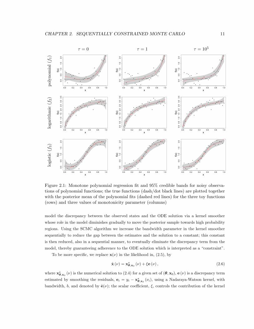
2.1 Monotone polynomial regression fit and 95% credible bands for noisy observations of
polynomial functions; the true functions (dash/dot black lines) are plotted together
with the posterior mean of the polynomial fits (dashed red lines) for the three toy
functions (rows) and three values of monotonicity parameter (columns) . . . . . . . 11
2.2 The SIR model- evolution of the posterior as a result of decreasing the coefficient, ξ. 14
2.3 The SIR model - joint posterior distribution of the model parameters for b = 26 and
ξ = 0. The three large clouds of particles correspond to I0 = 6, I0 = 5 and I0 = 4,
respectively, from left to right. . . . . . . . . . . . . . . . . . . . . . . . . . . . . . . 15
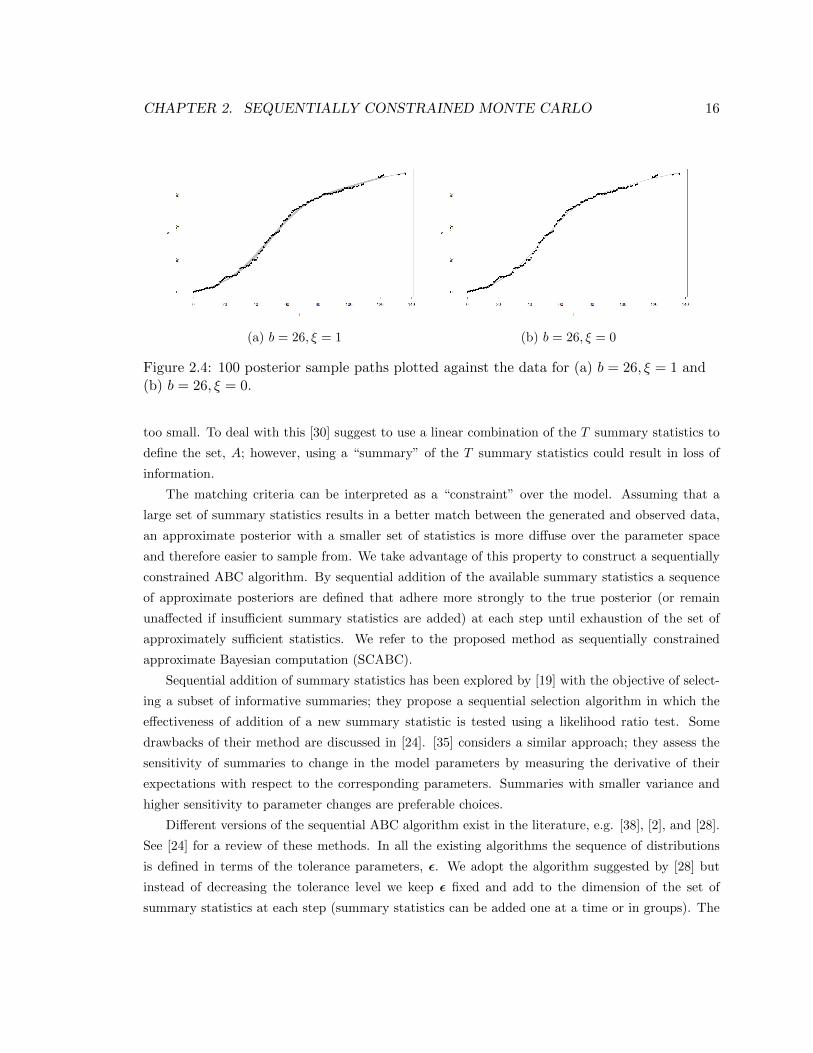
2.4 100 posterior sample paths plotted against the data for (a) b = 26, ξ = 1 and (b)
b = 26, ξ = 0. . . . . . . . . . . . . . . . . . . . . . . . . . . . . . . . . . . . . . . . . 16
2.5 The Ricker model- kernel density estimates of the approximate marginal posteriors
at times, t = 0, 1, . . . , T , the color of the curves grows darker with time; the dashed,
light gray curve is the prior density. The vertical lines are drawn at the true values of
the parameters. . . . . . . . . . . . . . . . . . . . . . . . . . . . . . . . . . . . . . . . 19
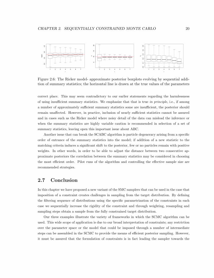
2.6 The Ricker model- approximate posterior boxplots evolving by sequential addition of
summary statistics; the horizontal line is drawn at the true values of the parameters 20
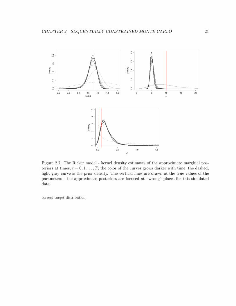
2.7 The Ricker model - kernel density estimates of the approximate marginal posteriors
at times, t = 0, 1, . . . , T , the color of the curves grows darker with time; the dashed,
light gray curve is the prior density. The vertical lines are drawn at the true values
of the parameters - the approximate posteriors are focused at “wrong” places for this
simulated data. . . . . . . . . . . . . . . . . . . . . . . . . . . . . . . . . . . . . . . . 21
3.1 Illustrative Example: (a) the true function plotted against x, the 7 evaluated points
of the function, and 100 sample paths taken from the GP posterior (b) posterior mean
and 95% credible intervals from the GP model together with the true function (c)
posterior mean and 95% credible intervals from the constrained model together with
the true function . . . . . . . . . . . . . . . . . . . . . . . . . . . . . . . . . . . . . . 31
xiii

3.2 Example 1. (a) GP mean and the probability of negative derivatives, (b) mean of the
GP derivative and the probability of negative derivatives. . . . . . . . . . . . . . . . 34
3.3 Example 1. The effect of sequential addition of derivative points on 95% credible
intervals; the posterior mean (dashed lines) and credible bands obtained by (a) un-
constrained GP model and (b-k) constrained models, together with the true function
(red lines) . . . . . . . . . . . . . . . . . . . . . . . . . . . . . . . . . . . . . . . . . . 35
3.4 Example 2. Input sets; training set (black), prediction set (letters), derivative set (red) 37
3.5 Example 2. Posterior mean and 95% credible intervals obtained by (a) unconstrained
GP model (b) GP model with monotonicity constraints; the red squares show the true
function values. . . . . . . . . . . . . . . . . . . . . . . . . . . . . . . . . . . . . . . 38
3.6 Simulation: examples of the polynomials with random coefficients generated from a
gamma(.01,1) . . . . . . . . . . . . . . . . . . . . . . . . . . . . . . . . . . . . . . . . 39
3.7 Simulation input sets; training set (black dots), prediction set (red squares), derivative
set (blue diamonds) . . . . . . . . . . . . . . . . . . . . . . . . . . . . . . . . . . . . 40
3.8 Simulation results: side by side boxplots of the (a) calculated RMSEs and (b) average
width of the 95% credible intervals for the unconstrained GP model and the monotone
model . . . . . . . . . . . . . . . . . . . . . . . . . . . . . . . . . . . . . . . . . . . . 41
3.9 queueing application: the average delay as a function of the two job arrival rates . . 43
3.10 Input sets; training set (black), prediction set (letters), derivative set (red) . . . . . . 44
3.11 Posterior mean and 95% credible intervals obtained by (a) unconstrained Bayesian
GP model (b) GP model with monotonicity constraints; the red squares show the
true function values. . . . . . . . . . . . . . . . . . . . . . . . . . . . . . . . . . . . . 45
3.12 Queueing application: Contours of the average delay as a function of job arrival
rates (gray) together with the input sets; training set (black), prediction set (letters),
derivative set (red) . . . . . . . . . . . . . . . . . . . . . . . . . . . . . . . . . . . . . 45
3.13 Posterior mean and 95% credible intervals obtained by (a) unconstrained Bayesian
GP model (b) GP model with monotonicity constraints; the red squares show the
true function values. . . . . . . . . . . . . . . . . . . . . . . . . . . . . . . . . . . . . 46
3.14 Example 2. Input sets; training set (black), prediction set (letters), derivative set (red) 49
3.15 Monotone emulation example; evolution of GP hyper-parameters; kernel density esti-
mates of the posterior at times t = 0, 1, . . . , T , the color of the curves grows darker
with time; the posterior means for times t = 0 (dahsed-black) and t = T (red) are
plotted for each parameter; (a) length scale in the first dimension (b) length scale in
the second dimension (c) variance parameter. . . . . . . . . . . . . . . . . . . . . . . 50
3.16 Monotone emulation example; evolution of predictions at points A-E; kernel density
estimates of the posterior predictive distribution at times t = 0, 1, . . . , T , the color of
the curves grows darker with time; the red vertical lines show the true function values. 50
xiv

3.17 The effect of sequential expansion of the derivative set on 95% credible intervals; the
posterior mean (dashed lines) and credible bands obtained by (a) unconstrained GP
model and (b) constrained model, together with the true function (red lines) . . . . 51
4.1 Local expected (dashed line) and observed (full line) p-values for a certain category
and all categories inclusive as a function of mass . . . . . . . . . . . . . . . . . . . . 54
4.2 The error rates (a) Exclusion type II error rate, β2, (b) γ1 and (c) γ2 plotted against
the signal sizes for the existing (solid line) and proposed (dashed line) procedures . 67
4.3 Data generated to imitate a specific channel of the real data together with background
(solid) and background plus signal (dashed) curves. The signal is centered at m =
126.5, the mass of the Higgs particle. . . . . . . . . . . . . . . . . . . . . . . . . . . . 70
4.4 Expected and observed local p-values in the log scale calculated based on a normal
approximation for the simulated data for the H → γγ channel. . . . . . . . . . . . . 71
4.5 Simulated Higgs analysis results; (a) prior pmf for the signal location, J , (b) estimated
posterior pmf for the signal location, J . . . . . . . . . . . . . . . . . . . . . . . . . . 72
4.6 Simulated Higgs data analysis results for the background function; prior 95% credible
bands (light grey), posterior 95% credible bands (dark grey) and posterior mean of
the background function (dashed curve). . . . . . . . . . . . . . . . . . . . . . . . . 73
A.1 Example 1. 95% credible intervals: (a) unconstrained GP model, (b) PAV algorithm,
(c) interpolating PAV algorithm, (d) monotone emulator . . . . . . . . . . . . . . . . 81
C.1 Power differences versus sJ averaged over s , for (a) n = 30, (b) n = 50, and (c) n = 100 85
xv
Chapter 1
Introduction
1.1 Overview
1.1.1 Constrained sequential Monte Carlo
In Bayesian inference, introduction of constraints into the model results in difficulties in sampling
from the posterior. Overcoming such difficulties were the motivation for development of a variant of
sequential Monte Carlo (SMC) that constitutes the first part of this thesis. SMC samplers, developed
by [27], take advantage of a sequence of distributions to filter a sample of parameter values (particles)
to obtain a sample from the target distribution that is the last distribution in the sequence. In our
version of SMC the filtering sequence is defined based on the constraints.
We apply the resulting sequentially constrained Monte Carlo (SCMC) approach in a variety of
frameworks where imposition of constraints creates challenging scenarios. We consider parameter
estimation for ordinary differential equations (ODE) where adherence of the model to the ODE
solution can be interpreted as a constraint. The other framework in which we use SCMC is approx-
imate Bayesian computation with a large collection of summary statistics that define a conservative
matching criterion resulting in problems in sampling efficiently. The SCMC algorithm is used for
efficient posterior sampling for montone emulation of computer experiements that is developed in
the second part of the thesis.
1.1.2 Monotone emulation of computer experiments
In computer experiments, a complex function is encoded into a deterministic and often computation-
ally intensive simulator. The domain of the function is referred to as the input space. The simulator
is run for a number of sampled inputs. A stochastic model, referred to as an emulator, is used to
predict the function at unsampled points in the input space. Due to the deterministic nature of the
1
CHAPTER 1. INTRODUCTION 2
simulator, the emulator is required to be an interpolator, i.e., it is expected to return the simulator
output if given the sampled input values. The emulator is also expected to provide uncertainty
estimates that satisfy the no-noise assumption at the sampled inputs. Gaussian processes (GP)
are commonly used in modeling computer experiments since they meet these requirements and are
flexible nonparametric models.
Sometimes, in addition to the computer simulator output, other information is available about
the underlying function in the form of constraints, e.g., positivity, monotonicity or convexity. In
this thesis, we consider the case that the underlying function is known to be monotone increasing or
decreasing and propose a method to incorporate this information into a GP to improve predictions.
The proposed methodology can also be applied in cases where a function is known to be positive or
to be convex.
The monotonicity information is introduced into the model using a “probabilistic truncation” on
the GP posterior that defines a soft constraint over the derivatives of the GP at a finite set of locations.
This amounts to encouraging local monotonicity rather than imposing universal monotonicity. The
effectiveness of the method is studied in one and two dimensional examples, a simulation study, and a
real application. The SCMC algorithm introduced in the first part of the thesis is used as a novel and
efficient computational approach that takes advantage of the parametrization of the monotonicity
constraint to facilitate posterior sampling.
1.1.3 Hypothesis testing in particle physics- search for the Higgs boson
The statistical procedures used for analysis of the data gathered from experiments performed in
a search for a new elementary particle are different from standard signal detection and hypothesis
testing procedures. The null and alternative hypotheses are defined such that the likelihood ratio
test (LRT) statistic should be modified to take into account the information provided by the theory
of quantum chromodynamics; this theory predicts the size and shape of the signal expected if the
sought-for particle exists. However, in the current practice this information is ignored and a standard
LRT is used.
Moreover, false discovery is penalized heavily in particle physics with type I error rates controlled
to remain at 3 × 10⁻⁷ ; this corresponds to a test statistic equivalent to a Z-score of 5. Physicists
describe this as a 5-σ test statistic. With such a small type I error rate, failure in detection is likely.
In this case the particle physicists are unwilling to stop their investigation; they switch the null and
alternative hypotheses and perform a set of LRTs that result in excluding ranges of mass values as
possible masses of the particle. Unlike the detection stage the type I error rates are only controlled
at 0.05 in the exclusion stage of the analysis..
This brief description of the existing procedure reveals a number of issues: firstly, certain im-
portant characteristics of the problem (the predicted signal strength in particular) are ignored to
facilitate standard statistical analysis; secondly, switching the null and alternative hypothesis is not

CHAPTER 1. INTRODUCTION 3
a common practice (it is possible only because of the signal strength is predicted by theory); and
finally, in the present application, the aspects of the problem that are ignored at the detection stage
are used in the exclusion stage.
These weaknesses of the current procedure were the motivation for development of a formal
statistical procedure that, while taking into account the important features of the problem, is able
to address the requirements and concerns, such as low false discovery rates that contribute to the
unusual structure of the existing procedure. We take a decision theoretic approach and define a
linear loss function that captures the possible scenarios and associates a loss with each case and
obtain the Bayes rule. A Bayesian hierarchical model is also proposed.
1.2 Organization
The rest of the thesis is organized as follows. In Chapter 2 we introduce the proposed variant of the
SMC sampleres after a brief review of the generic SMC and apply it to a few examples. In Chapter
3 monotone emulation of computer experiments is covered. Chapter 4 is dedicated to investigation
of the statistical procedures used in particle search problems. The thesis is concluded in Chapter 5.
Chapter 2
Sequentially Constrained Monte
Carlo
2.1 Introduction
In this chapter we develop a new variant of SMC samplers [27], that can be used in the case that
the difficulty in sampling from a target distribution, πT (θ), arises from imposition of a constraint
on the model which may also lead to cases where there are disagreements between the prior and
likelihood. We propose to connect the target distribution, πT (θ), to a “simple” distribution, π0(θ),
via a smooth path of distributions. We then do our computations by taking steps along this path so
that the constraints are enforced with increasing rigidity.
Constraints can be defined in a broad sense as any explicit restriction over the parameter space
or model space. A few examples are: inequality constraints over model parameters; monotonicity or
convexity of functions in functional data analysis; adherence of the stochastic model to a determin-
istic system, such as a system of differential equations; and a conservative acceptance criterion in
approximate Bayesian computation (ABC) defined to make the approximate posterior adhere closely
to the exact posterior. Examples of the last case are, small tolerance parameter or large number of
summary statistics used in matching the simulated and observed data.
To demonstrate the broad usage of our proposed variant of SMC in a variety of frameworks we ap-
ply the sequentially constrained Monte Carlo (SCMC) algorithm in different settings. To begin with
we use a toy problem to help understand and visualize the performance of the algorithm. We consider
polynomial regression fit to noisy observations of monotone functions. In sequentially imposing the
monotonicity information by defining a soft positivity constraint over the derivative polynomial, an
approach we will return to in Chapter 3, the predictions become more accurate while satisfying the
monotonicity constraints. In our second application we make Bayesian inference about the unknown
4

CHAPTER 2. SEQUENTIALLY CONSTRAINED MONTE CARLO 5
parameters and initial states of an ordinary differential equation model where we sequentially force
the model to adhere to the differential equation solution. The third example is focused on parameter
estimation for a chaotic dynamic system using approximate Bayesian computation. In this example,
available summary statistics are used sequentially to compare simulated and observed data.
2.2 Sequential Monte Carlo
SMC samplers are a family of algorithms that can be used in many challenging scenarios where
conventional Markov chain Monte Carlo (MCMC) methods fail in efficiently sampling from the
target distribution. SMC algorithms take advantage of a filtering sequence of distributions that
bridge between a distribution that is straightforward to sample from and the target distribution.
Suppose that πT (θ) is a target distribution that is difficult to sample from, for example, the
posterior distribution of the parameter vector, θ, in Bayesian inference. Let π0(θ) be a distribution
that can easily be generated from, for example the prior. SMC takes advantage of a family of
distributions, {πt}Tt=0, that bridge smoothly between π0 and πT ;
πt(θ) =ηt(θ)
Zt,
where Zt is the normalizing constant that may be unknown and ηt is a kernel that can be evaluated
for a given θ. Since the last distribution in the sequence is the target distribution the notation T
serves to indicate the target distribution as well as the number of steps in the sequential algorithm.
Starting from a sample of parameter values, referred to as particles, generated from π0, at time
t particles are moved and weighted according to the current distribution πt. Through iterative
importance sampling and resampling steps, particles are filtered along the sequence of distributions
to eventually obtain a sample from the target distribution.
Two common versions of SMC are based on gradually inducing the likelihood in the posterior.
Starting from a sample generated from the prior distribution, π(θ), for the vector of parameters,
θ, parameter values are shifted into samples from the posterior distribution, π(θ | y), with data,
y. In the first approach, the posterior is the only target distribution of interest and the likelihood
is tempered with the temperature parameters, 0 = τ0 < τ1 < . . . < τT = 1, giving rise to a power
posterior,
πt(θ | y) ∝ P (y | θ)τtπ(θ) (2.1)
The smooth path along {πt(θ | y)}Tt=0, is discretized where each resulting distribution becomes a
step along the sequential algorithm [27].
The second likelihood induction method, often referred to as particle filtering, has a natural
discretization where, in this case, the parameter defining the sequence, τ is used to denote inclusion
of the first τ data points. The tth sequential distribution, where 0 = τ0 ≤ τ1 ≤ . . . ≤ τT = N is given
CHAPTER 2. SEQUENTIALLY CONSTRAINED MONTE CARLO 6
Algorithm 1 Sequential Monte Carlo Sampler
Input: Forward and backward kernels, Kt(., .) and Lt(., .).1: Generate an initial sample θ1:N
0 ∼ π0;2: W j
0 ← 1N , j = 1, . . . , N ;
3: for t := 1, . . . , T do
• if ESS =
(∑Nj=1
(W jt−1
)2)−1
< N2 then
• resample θ1:Nt−1 with weights W 1:N
t−1
• W 1:Nt−1 ← 1
N
• end if
• Sample θ1:Nt ∼ Kt(θ
1:Nt−1, .);
• W jt ←W j
t−1wjt where wjt =
ηt(θjt )Lt−1(θj
t ,θjt−1)
ηt−1(θjt−1)Kt(θ
jt−1,θ
jt )
, j = 1, . . . , N ;
• Normalize W 1:Nt .
4: end forReturn: Particles θ1:N
1:T .
by:
πt(θ | y) ∝ P (y1, . . . ,yτt | θ)π(θ)
= P (yτt | θ)P (y1, . . . ,yτt−1 | θ)
∝ P (yτt | θ)πτt−1(θ | y).
(2.2)
This case works well for online estimation where data is available sequentially. The posterior defined
by the inclusion of all of the current data becomes the prior for the next stage of the algorithm where
more data becomes available. At each stage particles are moved towards the target posterior while
the target itself shifts at the next stage due to the inclusion of new data [11].
While SMC is mostly used in a Bayesian framework for posterior sampling, it can be generalized
as a Monte Carlo algorithm to generate from any target distribution. Therefore, although we work
in a Bayesian set-up in all our examples, to keep the notation simple and general, we denote the
target distribution by, πT (θ) and the filtering sequence by {πt}Tt=0.
We provide the original SMC algorithm, as given in [27], in Algorithm 1. This algorithm is very
general in the sense that many possible choices could be made for the inputs of the algorithm. The
choice of the inputs, especially the forward and backward kernels, Kt and Lt, can change the order
of the steps and result in different expressions for weights. A variety of options for the forward and
backward kernels and the resulting expressions for the incremental weights, wi, are provided in [27].
In the following, we explain the specific choices that are commonly made for all variants of SMC
that are introduced throughout the thesis.

CHAPTER 2. SEQUENTIALLY CONSTRAINED MONTE CARLO 7
Algorithm 2 Sequential Monte Carlo
Input: MCMC transition kernels Kt(., .).1: Generate an initial sample θ1:N
0 ∼ π0;2: W 1:N
1 ← 1N ;
3: for t := 1, . . . , T do
• W jt ←
wit∑wj
t
where wjt =ηt(θ
jt−1)
ηt−1(θjt−1)
, j = 1, . . . , N ;
• if ESS < N2 then
• resample θ1:Nt−1 with weights W 1:N
t−1 ;
• W 1:Nt−1 ← 1
N ;
• end if
• Sample θ1:Nt ∼ Kt(θ
1:Nt−1, .);
4: end forReturn: Particles θ1:N
1:T .
The forward kernels, Kt, are chosen to be MCMC kernels of invariant distributions, πt. The
backward kernels recommended in [27] for MCMC type forward kernels are,
Lt−1 =πt(θt−1)Kt(θt−1,θt)
πt(θt),
The above backward kernels are referred to as the “sub-optimal” backward kernels in [27] since they
are obtained by replacing the marginal importance distributions that do not have a closed form
representation by π in the optimal backward kernels. This choice of the forward and backward
kernels results in the simplified form of the incremental weights,
wjt =ηt(θ
jt−1)
ηt−1(θjt−1),
which means that the weights W 1:Nt are independent of θ1:Nt . In this case, the sampling step
is postponed until after the weights are evaluated and particles are resampled. Algorithm 2, a
transformed version of Algorithm 1 as the result of these specific choices, is the generic algorithm
that is used as a basis for all the algorithms tailored to our examples in the thesis.
Of advantages of SMC over MCMC is the facility of embarrassingly parallel computation; in
the time consuming steps of the algorithm, i.e., weight calculation and sampling, computation is
performed independently for each particle. Therefore, the sample can be split into batches where
computation for each batch is assigned to a different processor.
A common problem that can break the SMC algorithm is particle degeneracy. This term describes
a state in which most of the particles except a few acquire small or zero weights. The distance
between two consecutive distributions can play a role in particle degeneracy. The closer together
CHAPTER 2. SEQUENTIALLY CONSTRAINED MONTE CARLO 8
two distributions are in the sequence the lower is the chance of having small weights in resampling
since samples from the two distributions will then overlap. In Algorithm 2, the transition from one
distribution to the next in the sequence is done through the weighting and resampling steps. The
sampling step which moves the particles under the current distribution is an important step in this
case; low acceptance rate in sampling can result in particle degeneracy.
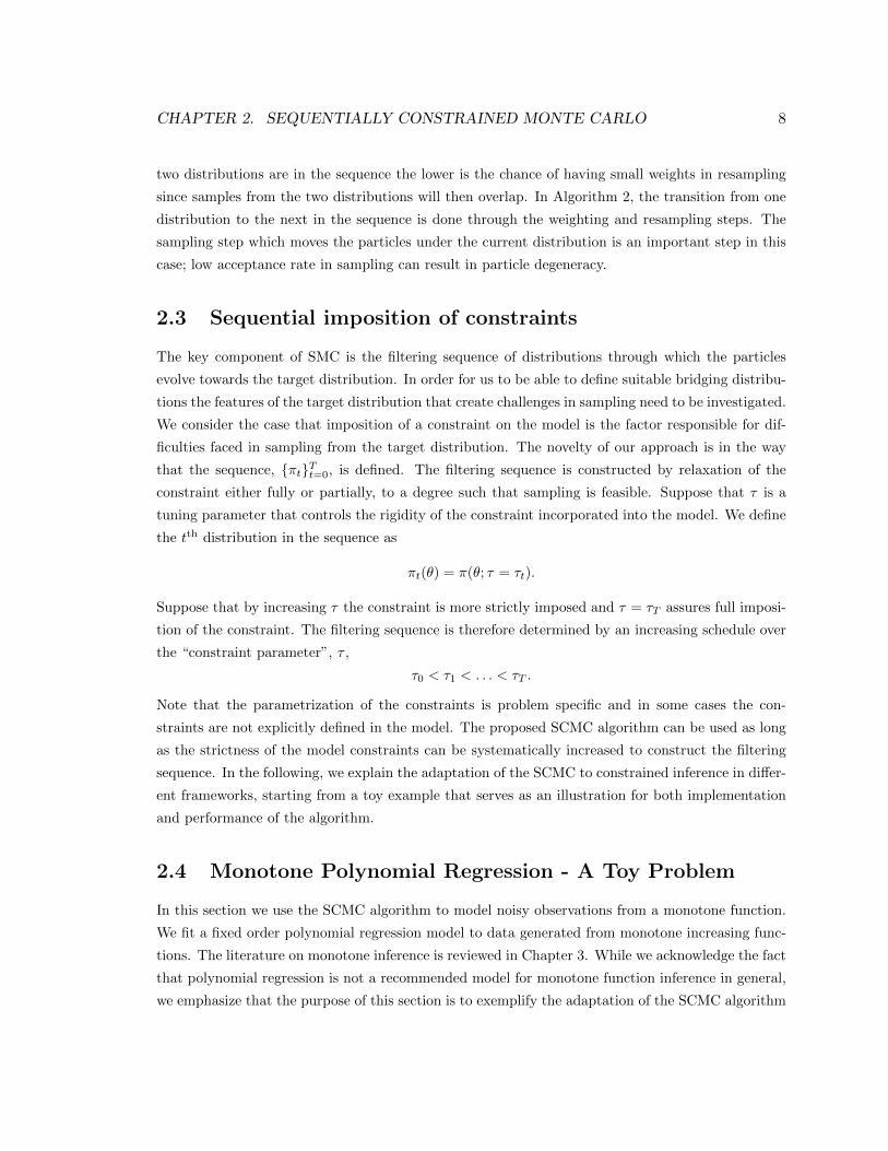
2.3 Sequential imposition of constraints
The key component of SMC is the filtering sequence of distributions through which the particles
evolve towards the target distribution. In order for us to be able to define suitable bridging distribu-
tions the features of the target distribution that create challenges in sampling need to be investigated.
We consider the case that imposition of a constraint on the model is the factor responsible for dif-
ficulties faced in sampling from the target distribution. The novelty of our approach is in the way
that the sequence, {πt}Tt=0, is defined. The filtering sequence is constructed by relaxation of the
constraint either fully or partially, to a degree such that sampling is feasible. Suppose that τ is a
tuning parameter that controls the rigidity of the constraint incorporated into the model. We define
the tth distribution in the sequence as
πt(θ) = π(θ; τ = τt).
Suppose that by increasing τ the constraint is more strictly imposed and τ = τT assures full imposi-
tion of the constraint. The filtering sequence is therefore determined by an increasing schedule over
the “constraint parameter”, τ ,
τ0 < τ1 < . . . < τT .
Note that the parametrization of the constraints is problem specific and in some cases the con-
straints are not explicitly defined in the model. The proposed SCMC algorithm can be used as long
as the strictness of the model constraints can be systematically increased to construct the filtering
sequence. In the following, we explain the adaptation of the SCMC to constrained inference in differ-
ent frameworks, starting from a toy example that serves as an illustration for both implementation
and performance of the algorithm.
2.4 Monotone Polynomial Regression - A Toy Problem
In this section we use the SCMC algorithm to model noisy observations from a monotone function.
We fit a fixed order polynomial regression model to data generated from monotone increasing func-
tions. The literature on monotone inference is reviewed in Chapter 3. While we acknowledge the fact
that polynomial regression is not a recommended model for monotone function inference in general,
we emphasize that the purpose of this section is to exemplify the adaptation of the SCMC algorithm
CHAPTER 2. SEQUENTIALLY CONSTRAINED MONTE CARLO 9
in a simple framework to help understand the implementation and the effectiveness of sequentially
constraining the model.
Let the data, y = (y1, . . . , yn)T
, be noisy observations of a monotone function, f , at x =
(x1, . . . , xn)T
. With no loss of generality, suppose that xi ∈ [0, 1]. Consider a pth-order polynomial
regression model,
y = Xβ + ε,
where
X =(1 x x2 · · · xp
);
and ε = (ε1, . . . , εn)T
are independent and identically distributed mean-zero normal random errors
with variance σ2.
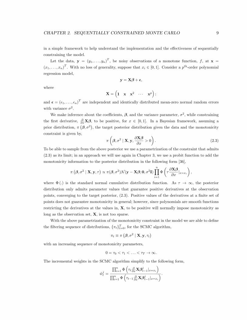
We make inference about the coefficients, β, and the variance parameter, σ2, while constraining
the first derivative, ∂∂xXβ, to be positive, for x ∈ [0, 1]. In a Bayesian framework, assuming a
prior distribution, π(β, σ2
), the target posterior distribution given the data and the monotonicity
constraint is given by,
π
(β, σ2 | X,y, ∂Xβ
∂x> 0
). (2.3)
To be able to sample from the above posterior we use a parametrization of the constraint that admits
(2.3) as its limit; in an approach we will use again in Chapter 3, we use a probit function to add the
monotonicity information to the posterior distribution in the following form [36],
π(β, σ2 | X,y, τ
)∝ π(β, σ2)N (y −Xβ;0, σ2I)
n∏i=1
Φ
(τ∂Xβ
∂x|x=xi
),
where Φ (.) is the standard normal cumulative distribution function. As τ → ∞, the posterior
distribution only admits parameter values that guarantee positive derivatives at the observation
points, converging to the target posterior, (2.3). Positive values of the derivatives at a finite set of
points does not guarantee monotonicity in general; however, since polynomials are smooth functions
restricting the derivatives at the values in, X, to be positive will normally impose monotonicity as
long as the observation set, X, is not too sparse.
With the above parametrization of the monotonicity constraint in the model we are able to define
the filtering sequence of distributions, {πt}Tt=0, for the SCMC algorithm,
πt ≡ π(β, σ2 | X,y, τt
)with an increasing sequence of monotonicity parameters,
0 = τ0 < τ1 < . . . < τT →∞.
The incremental weights in the SCMC algorithm simplify to the following form,
wjt =
∏ni=1 Φ
(τt
∂∂xXβ
jt−1|x=xi
)∏ni=1 Φ
(τt−1
∂∂xXβ
jt−1|x=xi
) .
CHAPTER 2. SEQUENTIALLY CONSTRAINED MONTE CARLO 10
Therefore we do not need to evaluate the likelihood in order to calculate the weights. This results
in more efficiency in computation.
With this choice of conjugate prior distributions the posterior distribution can be obtained
analytically [6] in the unconstrained case (τ = 0), thereby facilitating sampling from π0 at the first
step of the algorithm. The analytic unconstrained posterior is also used to define MCMC transition
kernels, Kt, for t = 1, . . . , T .
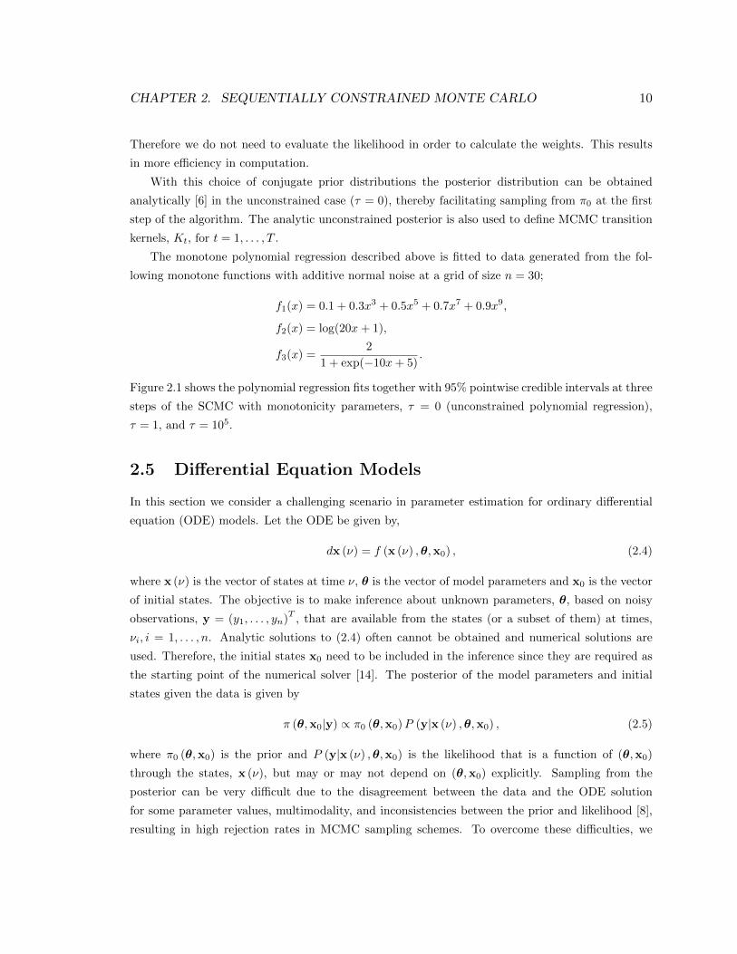
The monotone polynomial regression described above is fitted to data generated from the fol-
lowing monotone functions with additive normal noise at a grid of size n = 30;
f1(x) = 0.1 + 0.3x3 + 0.5x5 + 0.7x7 + 0.9x9,
f2(x) = log(20x+ 1),
f3(x) =2
1 + exp(−10x+ 5).
Figure 2.1 shows the polynomial regression fits together with 95% pointwise credible intervals at three
steps of the SCMC with monotonicity parameters, τ = 0 (unconstrained polynomial regression),
τ = 1, and τ = 105.
2.5 Differential Equation Models
In this section we consider a challenging scenario in parameter estimation for ordinary differential
equation (ODE) models. Let the ODE be given by,
dx (ν) = f (x (ν) ,θ,x0) , (2.4)
where x (ν) is the vector of states at time ν, θ is the vector of model parameters and x0 is the vector
of initial states. The objective is to make inference about unknown parameters, θ, based on noisy
observations, y = (y1, . . . , yn)T
, that are available from the states (or a subset of them) at times,
νi, i = 1, . . . , n. Analytic solutions to (2.4) often cannot be obtained and numerical solutions are
used. Therefore, the initial states x0 need to be included in the inference since they are required as
the starting point of the numerical solver [14]. The posterior of the model parameters and initial
states given the data is given by
π (θ,x0|y) ∝ π0 (θ,x0)P (y|x (ν) ,θ,x0) , (2.5)
where π0 (θ,x0) is the prior and P (y|x (ν) ,θ,x0) is the likelihood that is a function of (θ,x0)
through the states, x (ν), but may or may not depend on (θ,x0) explicitly. Sampling from the
posterior can be very difficult due to the disagreement between the data and the ODE solution
for some parameter values, multimodality, and inconsistencies between the prior and likelihood [8],
resulting in high rejection rates in MCMC sampling schemes. To overcome these difficulties, we
CHAPTER 2. SEQUENTIALLY CONSTRAINED MONTE CARLO 11
τ = 0 τ = 1 τ = 105p
olyn
omia
l(f
1)
0.0 0.2 0.4 0.6 0.8 1.0
0.0
0.5
1.0
1.5
2.0
x
f(x)
0.0 0.2 0.4 0.6 0.8 1.0
0.0
0.5
1.0
1.5
2.0
x
f(x)
0.0 0.2 0.4 0.6 0.8 1.0
0.0
0.5
1.0
1.5
2.0
x
f(x)
loga
rith
mic
(f2)
0.0 0.2 0.4 0.6 0.8 1.0
0.00.51.01.52.02.53.03.5
x
f(x)
0.0 0.2 0.4 0.6 0.8 1.0
0.00.51.01.52.02.53.03.5
x
f(x)
0.0 0.2 0.4 0.6 0.8 1.0
0.00.51.01.52.02.53.03.5
x
f(x)
logi
stic
(f3)
0.0 0.2 0.4 0.6 0.8 1.0
0.0
0.5
1.0
1.5
2.0
x
f(x)
0.0 0.2 0.4 0.6 0.8 1.0
0.0
0.5
1.0
1.5
2.0
x
f(x)
0.0 0.2 0.4 0.6 0.8 1.0
0.0
0.5
1.0
1.5
2.0
xf(x)
Figure 2.1: Monotone polynomial regression fit and 95% credible bands for noisy observa-tions of polynomial functions; the true functions (dash/dot black lines) are plotted togetherwith the posterior mean of the polynomial fits (dashed red lines) for the three toy functions(rows) and three values of monotonicity parameter (columns)
model the discrepancy between the observed states and the ODE solution via a kernel smoother
whose role in the model diminishes gradually to move the posterior sample towards high probability
regions. Using the SCMC algorithm we increase the bandwidth parameter in the kernel smoother
sequentially to reduce the gap between the estimates and the solution to a constant; this constant
is then reduced, also in a sequential manner, to eventually eliminate the discrepancy term from the
model, thereby guaranteeing adherence to the ODE solution which is interpreted as a “constraint”.
To be more specific, we replace x(ν) in the likelihood in, (2.5), by
x (ν) = xsθ,x0(ν) + ξe (ν) , (2.6)
where xsθ,x0(ν) is the numerical solution to (2.4) for a given set of (θ,x0), e (ν) is a discrepancy term
estimated by smoothing the residuals, ei = yi − xsθ,x0(νi), using a Nadaraya-Watson kernel, with
bandwidth, b, and denoted by e(ν); the scalar coefficient, ξ, controls the contribution of the kernel
CHAPTER 2. SEQUENTIALLY CONSTRAINED MONTE CARLO 12
smoother to the model. While for small b, x(ν) is nearly an interpolant and therefore accounts for
the discrepancy between the ODE solution and the data, as b gets larger to cover the whole range
of (ν0, νn), the model reduces to the ODE solution plus a constant, denoted by E, i.e.,
limb→∞
x (ν) = xsθ,x0(ν) + ξ lim
b→∞eb (ν)
= xsθ,x0(ν) + ξE.
In the next step, the limit is taken with respect to the coefficient ξ to eliminate the gap between the
estimated states and the ODE solution;
limξ→0
limb→∞
x (ν) = xsθ,x0(ν) + lim
ξ→∞ξE
= xsθ,x0(ν) .
The above model is fitted to the data using the SCMC algorithm by defining a sequence of
models initially corresponding to an increasing schedule over the bandwidth parameter, b, while ξ is
held fixed at 1, and next a decreasing schedule over the coefficient, ξ, with the bandwidth held fixed
at a large value. That is, the tth distribution in the filtering sequence is given by
πt ∝ π0 (θ,x0)P (y|xbt,ξt (ν) ,θ,x0) .
for
b0 < b1 < . . . < bt∗ = bt∗+1 = . . . = bT ,
and
1 = ξ0 = ξ1 = . . . = ξt∗ > ξt∗+1 > . . . > ξT = 0.
We choose a Susceptible-Infected-Recovered (SIR) epidemiological model to illustrate the adap-
tation of SCMC to the model, (2.6). A population of size N comprises the susceptibles, S, infected,
I, and removed, R, individuals. The disease spread rate is modeled as follows,dS (ν) = −βS (ν) I (ν)
dI (ν) = βS (ν) I (ν)− αI (ν)
dR (ν) = αI (ν)
(2.7)
where the parameters, α and β, as well as the initial state, I0, are unknown. At time 0 the population
only consists of susceptible and infectious individuals therefore we have, R0 = 0 and S0 = N − I0.
The data, y = {y1, . . . , yn}, are the number of deaths observed up to times, {ν1, . . . , νn}. We define
the likelihood as,
P (y | Rα,β,I0(ν)) =
n∏i=1
(N
yi
)(Rα,β,I0 (νi)
N
)yi (1− Rα,β,I0 (νi)
N
)(N−yi)
.
CHAPTER 2. SEQUENTIALLY CONSTRAINED MONTE CARLO 13
We acknowledge that the assumption of independence between the number of deaths, used to con-
struct the likelihood, is not realistic. However, the basic behavior of the ODE is captured in this
likelihood through the drifting binomial means. To evaluate the likelihood for each set of parameters
and initial states, we need to estimate the states, Rα,β,I0 , which as described above are obtained by
fitting a kernel smooth to the residuals,
ei = yi −Rsα,β,I0 (νi) ,
where Rsα,β,I0 (νi) is obtained by numerically solving (2.7).
Following [7], prior distributions for α and β are chosen to be gamma (1, 1). The prior distribution
of the initial state, I0, is chosen to be a binomial distribution with parameters N and 5/N . Having
both discrete and continuous parameters in the model compounds the difficulty of sampling from the
posterior; MCMC can easily get trapped in local modes of the posterior surface in this case. These
challenges are overcome by the SCMC which is based on importance sampling schemes rather than
random-walk-based techniques.
The model described above is fitted to a data set, also used in [7], which are daily counts of deaths
from the second outbreak of the plague from June 19, 1666 until November 1, 1666 in the village of
Eyam, UK, as recorded by the town gravedigger [25]. The number of observations is n = 136 and
the total population of the village is N = 261.
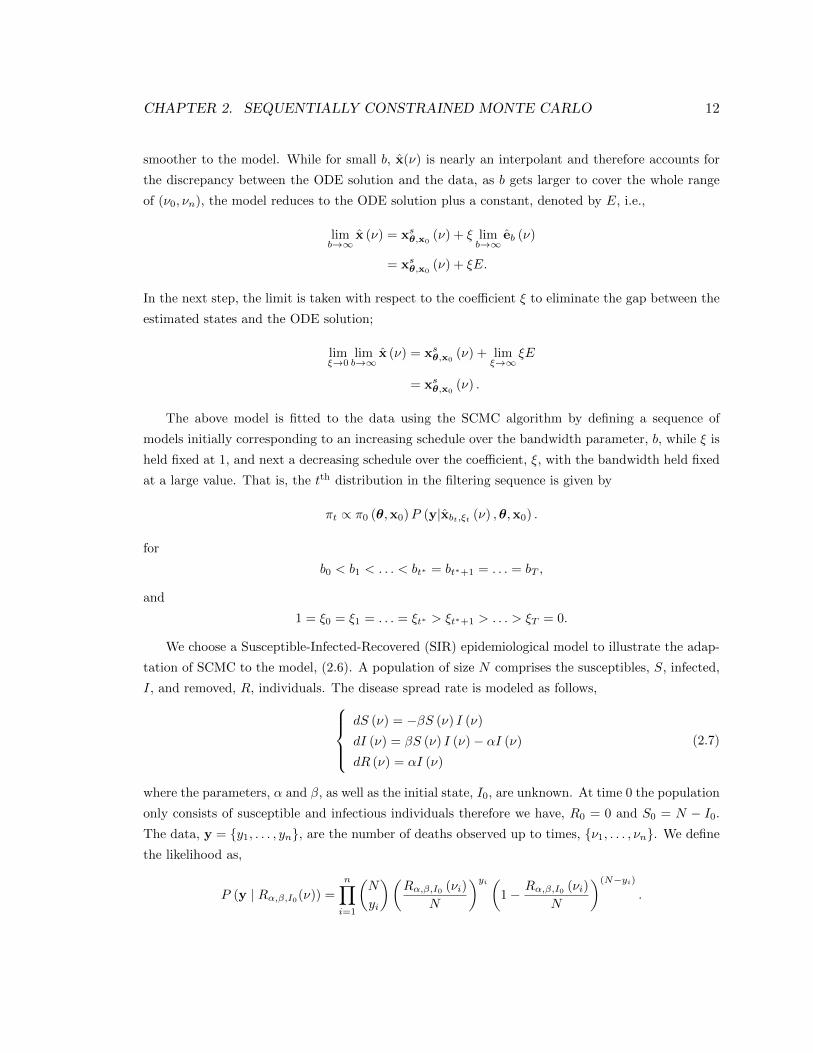
Figures 2.2a, 2.2b and 2.2c present the results of fitting the model, (2.6), to these data in the
form of the joint posterior samples of the model parameters, α and β, for three increasing values of
the bandwidth parameter, b, while the coefficient is held fixed at ξ = 1. The parameter values are
distributed in the shape of a boomerang in Figure 2.2b. The lower part of the boomerang refers to
the contribution of the kernel smoother to the model, i.e., the parameter values whose corresponding
states are non-smooth and deviate from the ODE solution and this deviation is accounted for by the
smoother. By increasing the bandwidth, the smoother reduces to a constant and the corresponding
parameter values are filtered out of the posterior sample.
Figures 2.2d, 2.2e and 2.2f show the joint posterior samples for the model parameters for the
proceeding steps of the sampler where the bandwidth is held fixed at b = 26, but the coefficient, ξ,
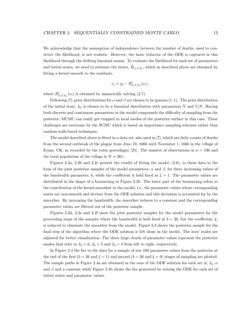
is reduced to eliminate the smoother from the model. Figure 2.3 shows the posterior sample for the
final step of the algorithm where the ODE solution is left alone in the model. The axes’ scales are
adjusted for better visualization. The three large clouds of parameter values represent the posterior
modes that refer to I0 = 6, I0 = 5 and I0 = 4 from left to right, respectively.
In Figure 2.4 the fits to the data for a sample of size 100 parameter values from the posterior at
the end of the first (b = 26 and ξ = 1) and second (b = 26 and ξ = 0) stages of sampling are plotted.
The sample paths in Figure 2.4a are obtained as the sum of the ODE solution for each set of, I0, α
and β and a constant while Figure 2.4b shows the fits generated by solving the ODE for each set of
initial states and parameter values.
CHAPTER 2. SEQUENTIALLY CONSTRAINED MONTE CARLO 14
(a) b = 2, ξ = 1 (b) b = 12, ξ = 1 (c) b = 20, ξ = 1
(d) b = 26, ξ = 0.95 (e) b = 26, ξ = 0.5 (f) b = 26, ξ = 0
Figure 2.2: The SIR model- evolution of the posterior as a result of decreasing the coefficient,ξ.
2.6 Sequentially Constrained Approximate Bayesian Compu-
tation
Approximate Bayesian computation (ABC) methods [39] were proposed for Bayesian inference in
cases where the likelihood is intractable or expensive to evaluate but can be generated from. Samples
from the approximate posterior are obtained by simulating pseudo-data from the likelihood for
any given set of model parameters and “matching” the simulated data with the observed data. If
parameter values satisfy the “matching criteria” they are included in the posterior sample, otherwise
they are excluded.
Suppose that y is the observed data, θ is the vector of parameters and the likelihood is denoted
by P (y|θ). The target approximate posterior distribution is given by,
πA (θ, z|y) =π (θ)P (z|θ)1A (z)∫Aπ (θ)P (z | θ) dz
,
where z is the simulated data and A is the set of matching criteria. In the simplest version of the
ABC algorithm, parameter values, θ∗, are generated from the prior; pseudo-data, z, are generated
from the likelihood, P (z|θ∗); if z ∈ A, θ∗ is accepted as a sample value from the posterior and it is
otherwise rejected.
The matching criteria, defining the set A, are a measure of similarity between the simulated
and observed data. They would ideally be defined based on equality (for discrete distributions) or
CHAPTER 2. SEQUENTIALLY CONSTRAINED MONTE CARLO 15
0.00055 0.00060 0.00065 0.00070
0.08
50.
095
0.10
5
β
α
Figure 2.3: The SIR model - joint posterior distribution of the model parameters for b = 26and ξ = 0. The three large clouds of particles correspond to I0 = 6, I0 = 5 and I0 = 4,respectively, from left to right.
closeness (for continuous distributions) of sufficient statistics, s, i.e.,
Ay = {z|s (z) = s (y)}
in the discrete case or
Ay = {z|ρ (s (z) , s (y)) < ε}
in the continuous case, where ρ is a distance measure and ε is a tolerance level.
In practice non-trivial sufficient statistics are rarely known. Instead, a collection of “approxi-
mately sufficient” statistics, η (y) = (η1 (y) , . . . , ηT (y))T
, are used to examine the goodness of the
match. When one is uncertain about an optimal subset of summary statistics, a recommended strat-
egy is to use as many summary statistics as are available since in principle adding statistics that
contain no information about the parameters does not affect the posterior. The matching criteria in
this case are defined as,
Aε,y = {z|ρ (η1 (z) , η1 (y)) < ε1, . . . , ρ (ηT (z) , ηT (y)) < εT },
where ε = (ε1, . . . , εT ) is a vector of tolerance levels.
In practice, however, the dimensionality of the set of summary statistics can result in difficulties
in posterior sampling. To be more specific, fewer parameter values are accepted when the acceptance
criteria, A, is too conservative either because the dimension T is too large or the tolerances εi are
CHAPTER 2. SEQUENTIALLY CONSTRAINED MONTE CARLO 16
(a) b = 26, ξ = 1 (b) b = 26, ξ = 0
Figure 2.4: 100 posterior sample paths plotted against the data for (a) b = 26, ξ = 1 and(b) b = 26, ξ = 0.
too small. To deal with this [30] suggest to use a linear combination of the T summary statistics to
define the set, A; however, using a “summary” of the T summary statistics could result in loss of
information.
The matching criteria can be interpreted as a “constraint” over the model. Assuming that a
large set of summary statistics results in a better match between the generated and observed data,
an approximate posterior with a smaller set of statistics is more diffuse over the parameter space
and therefore easier to sample from. We take advantage of this property to construct a sequentially
constrained ABC algorithm. By sequential addition of the available summary statistics a sequence
of approximate posteriors are defined that adhere more strongly to the true posterior (or remain
unaffected if insufficient summary statistics are added) at each step until exhaustion of the set of
approximately sufficient statistics. We refer to the proposed method as sequentially constrained
approximate Bayesian computation (SCABC).
Sequential addition of summary statistics has been explored by [19] with the objective of select-
ing a subset of informative summaries; they propose a sequential selection algorithm in which the
effectiveness of addition of a new summary statistic is tested using a likelihood ratio test. Some
drawbacks of their method are discussed in [24]. [35] considers a similar approach; they assess the
sensitivity of summaries to change in the model parameters by measuring the derivative of their
expectations with respect to the corresponding parameters. Summaries with smaller variance and
higher sensitivity to parameter changes are preferable choices.
Different versions of the sequential ABC algorithm exist in the literature, e.g. [38], [2], and [28].
See [24] for a review of these methods. In all the existing algorithms the sequence of distributions
is defined in terms of the tolerance parameters, ε. We adopt the algorithm suggested by [28] but
instead of decreasing the tolerance level we keep ε fixed and add to the dimension of the set of
summary statistics at each step (summary statistics can be added one at a time or in groups). The
CHAPTER 2. SEQUENTIALLY CONSTRAINED MONTE CARLO 17
sequence of approximate posterior distributions, {πAt}Tt=1, is defined based on a decreasing sequence
of acceptance sets,
A1 ⊇ A2 ⊇ . . . ⊇ AT ,
where
At = {z|ρ (η1 (z) , η1 (y)) < ε1, . . . , ρ (ητt (z) , ητt (y)) < ετt}.
The constraint parameter in this case is the number of summary statistics included up to time t,
τt. The tolerance levels, {εj}τTj=1, are obtained as small quantiles of the empirical distribution of
ρ (ηj (z) , ηj (y)) prior to running the algorithm and as mentioned above, are held fixed. However,
if needed, the filtering sequence may be defined based on a combination of decreasing tolerance
parameters and increasing number of summary statistics.
Algorithm 3 outlines the SCABC algorithm that generates parameter values according to a
sequence of approximate posterior distributions constructed as described above. In the following, we
apply Algorithm 3 to simulated data from a chaotic dynamic model to illustrate the effectiveness of
sequential enforcement of the constraints in the ABC framework.
We consider the chaotic ecological dynamic system, referred to as the Ricker map [40], that is
used by [43] in a related framework. As explained by [43], likelihood-based inference breaks down for
chaotic dynamics since small changes in the system parameters produce large changes in the system
states later in time; therefore the likelihood does not depend smoothly on the parameters. Also these
systems are only observable with error. Alternatively, [43] propose a synthetic likelihood constructed
based on a set of summary statistics that capture the important dynamics in the data rather than
the noise-driven detail. Borrowing the Ricker example and some of our summary statistics from [43],
we employ the SCABC algorithm, described above, to make inference about the model parameters.
The scaled Ricker map describes the dynamics of a discrete population, Nν , over time as,
Nν+1 = rNν exp (−Nν + eν),
where eν are independent normal errors with mean zero and variance, σ2e , that represent the process
noise, and r is the growth rate parameter. The data are the outcome of a Poisson distribution
observed at n = 50 time steps,
y ∼ Poisson (φNν) ,
where φ is a scaling parameter. The vector of parameters that inference is made about is given by
θ =(r, σ2
e , φ)T
. The likelihood, P (y|θ), which is obtained by integrating over eν is analytically and
numerically intractable [9], thereby, raising the demand for a likelihood-free approach. The summary
statistics used in the SCABC algorithm are,
η =
(med(y),
∑ni=1 yin
,
∑ni=1 y1(1,∞)(yi)∑ni=1 1(1,∞)(yi)
,
n∑i=1
yi1(10,∞)(yi),
n∑i=1
1{0}(yi), Q0.75(y),max(y)
)T
CHAPTER 2. SEQUENTIALLY CONSTRAINED MONTE CARLO 18
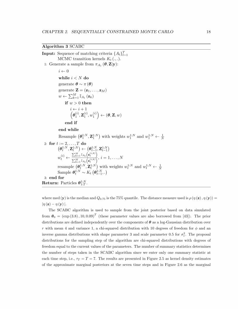
Algorithm 3 SCABC
Input: Sequence of matching criteria {At}Tt=1
MCMC transition kernels Kt (., .).1: Generate a sample from πA1 (θ,Z|y):
i← 0
while i < N do
generate θ ∼ π (θ)
generate Z = (z1, . . . , zM )
w ←∑M
k=1 IA1 (zk)
if w > 0 then
i← i+ 1(θ
(i)1 ,Z
(i)1 , w
(i)1
)← (θ,Z, w)
end if
end while
Resample(θ1:N
1 ,Z1:N1
)with weights w1:N
1 and w1:N1 ← 1
N
2: for t := 2, . . . , T do(θ1:Nt ,Z1:N
t
)←(θ1:Nt−1,Z
1:Nt−1
)w
(i)t ←
∑Mk=1 IAt
(z(i,k)t
)∑M
k=1 IAt
(z(i,k)t
) , i = 1, . . . , N
resample(θ1:Nt ,Z1:N
t
)with weights w1:N
t and w1:Nt ← 1
N
Sample θ1:Nt ∼ Kt
(θ1:Nt−1, .
)3: end for
Return: Particles θ1:N1:T .
where med (y) is the median andQ0.75 is the 75% quantile. The distance measure used is ρ (η (z) , η (y)) =
|η (z)− η (y) |.The SCABC algorithm is used to sample from the joint posterior based on data simulated
from θ0 = (exp (3.8) , 10, 0.09)T
(these parameter values are also borrowed from [43]). The prior
distributions are defined independently over the components of θ as a log-Gaussian distribution over
r with mean 4 and variance 1, a chi-squared distribution with 10 degrees of freedom for φ and an
inverse gamma distributions with shape parameter 3 and scale parameter 0.5 for σ2e . The proposal
distributions for the sampling step of the algorithm are chi-squared distributions with degrees of
freedom equal to the current values of the parameters. The number of summary statistics determines
the number of steps taken in the SCABC algorithm since we enter only one summary statistic at
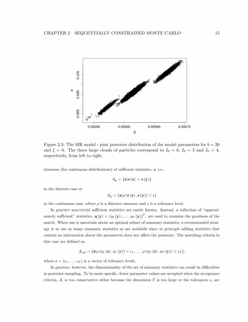
each time step, i.e., τT = T = 7. The results are presented in Figure 2.5 as kernel density estimates
of the approximate marginal posteriors at the seven time steps and in Figure 2.6 as the marginal
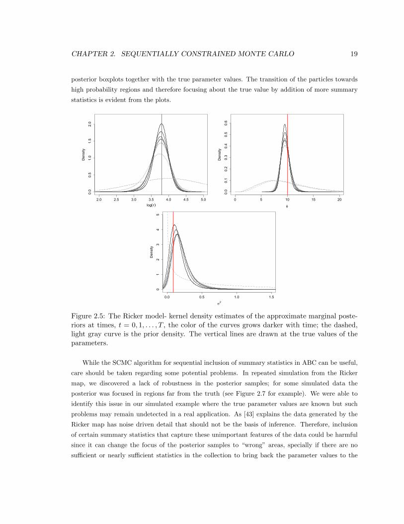
CHAPTER 2. SEQUENTIALLY CONSTRAINED MONTE CARLO 19
posterior boxplots together with the true parameter values. The transition of the particles towards
high probability regions and therefore focusing about the true value by addition of more summary
statistics is evident from the plots.
2.0 2.5 3.0 3.5 4.0 4.5 5.0
0.0
0.5
1.0
1.5
2.0
log(r)
Density
0 5 10 15 20
0.0
0.1
0.2
0.3
0.4
0.5
0.6
f
Density
0.0 0.5 1.0 1.5
01
23
45
s2
Density
Figure 2.5: The Ricker model- kernel density estimates of the approximate marginal poste-riors at times, t = 0, 1, . . . , T , the color of the curves grows darker with time; the dashed,light gray curve is the prior density. The vertical lines are drawn at the true values of theparameters.
While the SCMC algorithm for sequential inclusion of summary statistics in ABC can be useful,
care should be taken regarding some potential problems. In repeated simulation from the Ricker
map, we discovered a lack of robustness in the posterior samples; for some simulated data the
posterior was focused in regions far from the truth (see Figure 2.7 for example). We were able to
identify this issue in our simulated example where the true parameter values are known but such
problems may remain undetected in a real application. As [43] explains the data generated by the
Ricker map has noise driven detail that should not be the basis of inference. Therefore, inclusion
of certain summary statistics that capture these unimportant features of the data could be harmful
since it can change the focus of the posterior samples to “wrong” areas, specially if there are no
sufficient or nearly sufficient statistics in the collection to bring back the parameter values to the
CHAPTER 2. SEQUENTIALLY CONSTRAINED MONTE CARLO 20
1 2 3 4 5 6 7
3.0
3.5
4.0
4.5
t
log(r)
1 2 3 4 5 6 7
510
1520
t
f
1 2 3 4 5 6 7
0.0
0.1
0.2
0.3
0.4
0.5
t
s e
Figure 2.6: The Ricker model- approximate posterior boxplots evolving by sequential addi-tion of summary statistics; the horizontal line is drawn at the true values of the parameters
correct place. This may seem contradictory to our earlier statements regarding the harmlessness
of using insufficient summary statistics. We emphasize that that is true in principle, i.e., if among
a number of approximately sufficient summary statistics some are insufficient, the posterior should
remain unaffected. However, in practice, inclusion of nearly sufficient statistics cannot be assured
and in cases such as the Ricker model where noisy detail of the data can mislead the inference or
when the summary statistics are highly variable caution is recommended in selection of a set of
summary statistics, leaving open this important issue about ABC.
Another issue that can break the SCABC algorithm is particle degeneracy arising from a specific
order of entrance of the summary statistics into the model; if addition of a new statistic to the
matching criteria induces a significant shift to the posterior, few or no particles remain with positive
weights. In other words, in order to be able to adjust the distance between two consecutive ap-
proximate posteriors the correlation between the summary statistics may be considered in choosing
the most efficient order. Pilot runs of the algorithm and controlling the effective sample size are
recommended strategies.
2.7 Conclusion
In this chapter we have proposed a new variant of the SMC samplers that can be used in the case that
imposition of a constraint creates challenges in sampling from the target distribution. By defining
the filtering sequence of distributions using the specific parametrization of the constraints in each
case we sequentially increase the rigidity of the constraint and through weighting, resampling and
sampling steps obtain a sample from the fully constrained target distribution.
Our three examples illustrate the variety of frameworks in which the SCMC algorithm can be
used. This wide scope of application is due to our broad interpretation of constraints; any restriction
over the parameter space or the model that could be imposed through a number of intermediate
steps can be assembled in the SCMC to provide the means of efficient posterior sampling. However,
it must be assured that the formulation of constraints is in fact leading the sampler towards the
CHAPTER 2. SEQUENTIALLY CONSTRAINED MONTE CARLO 21
2.0 2.5 3.0 3.5 4.0 4.5 5.0
0.0
0.5
1.0
1.5
2.0
log(r)
Density
0 5 10 15 20
0.0
0.2
0.4
0.6
0.8
f
Density
0.0 0.5 1.0 1.5
01
23
45
s2
Density
Figure 2.7: The Ricker model - kernel density estimates of the approximate marginal pos-teriors at times, t = 0, 1, . . . , T , the color of the curves grows darker with time; the dashed,light gray curve is the prior density. The vertical lines are drawn at the true values of theparameters - the approximate posteriors are focused at “wrong” places for this simulateddata.
correct target distribution.
Chapter 3
Monotone Emulation of Computer
Experiments
3.1 Introduction
Deterministic computer models are commonly used to study complex physical phenomena in many
areas of science and engineering. Oftentimes, evaluating a computational model can be very time
consuming, and thus the simulator is only exercised on a relatively small set of input values. In such
cases, a statistical surrogate model (i.e., an emulator) is used to make predictions of the computer
model output at unsampled inputs. Gaussian process (GP) models are popular choices for deter-
ministic computer model emulation [37]. The reason for this rests on the flexibility of the GP as
explained in Chapter 2, its adaptability to the noise-free framework and its ability to provide a basis
for statistical inference for deterministic computer models.
The properties of GP derivatives make them attractive in some settings. Indeed, when the
simulator output includes derivatives, they can be used to improve the efficiency of the emulator [29].
In some applications derivative information is available only in the form of qualitative information
- for example, the computer model response is known to be monotone increasing or decreasing in
some of the inputs. Incorporating the derivative information into the emulator in such cases is more
challenging because the derivative values themselves are unknown. The problem of using the known
monotonicity of the computer model response in one or more of the inputs to build a more efficient
emulator is the main focus of this chapter.
While a rich literature exists on monotone function estimation, interpolation of monotone func-
tions with uncertainty quantification remains an understudied topic. Examples of related work are
monotone smoothing splines, isotonic regression, etc. (See for e.g. [32], [16] and [10].) Also work has
been done on incorporating constraints, in general, and monotonicity specially, into Gaussian process
22
CHAPTER 3. MONOTONE EMULATION OF COMPUTER EXPERIMENTS 23
regression as discussed below. In a related framework, constrained kriging has been considered in
the area of geostatistics [20]. While some of the existing methods may be modified to be used in the
noise-free set-up none of them directly address monotone interpolation. On the other hand, there
exist tools for monotone interpolation that do not provide uncertainty estimates (e.g. [42]).
Monotonicity assumptions in GP models for noisy data are considered in [36]. They incor-
porate the monotonicity information by placing virtual derivatives at pre-specified input locations
and encouraging the derivative process to be positive at these points using a probit link function.
Expectation-propagation techniques [26] are used to approximate the joint marginal likelihood of
function and derivative values. Point estimates for the hyperparameters are obtained by maximizing
this approximate likelihood.
A related Bayesian approach to monotone estimation of GP models has been independently
developed in [41]. Similar to the method explained in this chapter, the sign of derivatives at user-
specified locations is assumed known. Two modeling approaches are taken: i) an indicator variable
formulation, which can be seen as a limiting case of a probit link of [36] (also used in this chapter),
and ii) a conditional GP model, which allows zero or positive derivative values. [41] uses plug-in point
estimates of GP parameters and demonstrates applications with no more than one input dimension.
[41] considers the extension to higher-order derivatives.
[22] propose a GP based method for estimating monotone functions that relies on projecting
sample paths obtained from a GP fit to the space of monotone functions. They use the pooled
adjacent violators (PAV) algorithm to obtain approximate projections. While the projections of
interpolating GP sample paths into the space of monotone functions are not generally guaranteed
to interpolate the function evaluations, the PAV algorithm can be modified to generate monotone
interpolants. However, there are two drawbacks to this method; firstly, inference cannot be made
about the model parameters by projecting GP sample paths since it is not trivial how the posterior
distribution of the covariance parameters is affected by the projection. Secondly, sample paths
generated by the PAV algorithm are often non-smooth since monotonicity is gained by flattening
the ridges and valleys resulting in flat segments followed by occasional rises. The “box-like” credible
intervals obtained from the projected interpolants are truncated from below and above to exclude
violating sample paths resulting in lack of interpretability arising from the fact that the credible
intervals remain unchanged for a range of coverage probabilities. In Appendix A we apply this
method to one of our examples and compare the results.
The novelty of our approach as well as the modifications/improvements made to the previous
work on this topic can be summarized as follows. We initially take an approach similar to [36] to
build an emulator, given the computer model output and monotonicity information. Our approach
is different from the existing work mentioned above in two respects. First, we focus on deterministic
computer experiments where interpolation of the simulator is a requirement. Constructing a mono-
tone emulator is more challenging in the deterministic setting than the noisy setting. The problem
CHAPTER 3. MONOTONE EMULATION OF COMPUTER EXPERIMENTS 24
in our case lies in generating sample paths from the GP that obey monotonicity and also interpolate
the simulator output. In the noisy setting, where the GP need not interpolate the observations,
sampling from the GP is easier. Second, we sample from the exact joint posterior distribution of
the function, derivatives and hyperparameters rather than relying on an approximate likelihood and
plug-in point estimates. In doing so, we provide fully Bayesian inference for the parameters of the
emulator as well as the predicted function at unsampled inputs, thereby addressing the uncertainty
associated with these parameters. We also take advantage of the flexible parametrization of mono-
tonicity information to facilitate efficient computation. A variant of the sequential Monte Carlo
samplers that was introduced in Chapter 2 is used that permits sampling from the full posterior in
fairly high-dimensional scenarios.
We show that when the monotonicity constraints are more strict, the support of the distribution
for the derivatives gets restricted to <+. The end result of the proposed approach is an emulator of
the computer model that uses the monotonicity information and is more efficient than the standard
GP. We demonstrate the performance of the methodology in examples with more than one input
dimension and a two-dimensional real application.
3.2 Gaussian process models
Gaussian processes are nonparametric models that are extensively used in various areas of statistics
for modeling unknown functions. Let y : <d → < be a function we wish to infer, where d is the
number of inputs. A Gaussian process prior is assumed for y denoted by,
y(x) ∼ GP(µ(x), ρ(x,x′)), (3.1)
where x = (x1, . . . , xd) and x′ = (x′1, . . . , x′d) are two arbitrary points in the input space, <d, and
µ(x) and ρ(x,x), are the prior mean and covariance functions, respectively. The mean function may
be a constant, e.g., µ(x) = 0, a known function, e.g., µ(x) = g(x), or a function with unknown
parameters, µ(x) = gβ(x), where β are estimated among the GP hyper-parameters.
The flexibility of GP is due to the wide range of covariance structures that could be used. For
examples of covariance functions see [34]. In this thesis, we use anisotropic, stationary, product form
covariance functions,
ρ(x,x′) = σ2d∏k=1
ξ(|xk − x′k|
lk), (3.2)
where ξ(δ) is decreasing in δ, the variance parameter, σ2, controls the variability of the GP prior,
and l = (l1, . . . , ld) is the vector of length scale parameters where lk controls the smoothness of the
prior GP in the kth dimension.
By definition, if y is a GP, for any finite set of points, denoted by X = (x1, . . . ,xn)T ,
y(X) ∼ Nn(µ,Σ),
CHAPTER 3. MONOTONE EMULATION OF COMPUTER EXPERIMENTS 25
where Nn is the n-variate Gaussian distribution with mean vector
µ =
µ(x1)
...
µ(xn)
,
and covariance matrix
Σ =
ρ(x1,x1) ρ(x1,x2) . . . ρ(x1,xn)
ρ(x2,x1) ρ(x2,x2) . . . ρ(x2,xn)...
.... . .
...
ρ(xn,x1) ρ(xn,x2) . . . ρ(xn,xn)
.
Suppose that the data, y = (y1, . . . , yn), are assumed to be a stochastic realization of y at a
number of input locations, X, i.e., the likelihood is a parametric distribution in y,
y ∼ P (y|y(X)). (3.3)
The posterior of y given y at any point x∗ is given by;
π(y(x∗)|y) =
∫π(y(x∗), y(X)|y)dy(X), (3.4)
where
π(y(x∗), y(X)|y) ∝ π(y(x∗), y(X))P (y|y(X)),
and
π(y(x∗), y(X)) = Nn+1(µ′,Σ′),
where
µ′ =
(µ
µ(x∗)
),
and
Σ′ =
(Σ ρ
ρT ρ(x∗,x∗)
). (3.5)
where ρ is a n× 1 vector whose ith element is ρ(xi,x∗).
3.2.1 Special Cases
Gaussian Likelihood
In the case that the likelihood, (3.3), is a Gaussian distribution, i.e.,
y ∼ N (y(X),Σy),
CHAPTER 3. MONOTONE EMULATION OF COMPUTER EXPERIMENTS 26
by conjugacy, the posterior, (3.4), is given by a GP,
y(x)|y ∼ GP(µ′(x), ρ′(x,x′)). (3.6)
with mean function,
µ′(x) = µ(x) + ρTR−1y,
and covariance function,
ρ′(x,x′) = ρ(x,x′)− ρTR−1ρ.
where R = Σ + Σy.
Noise-free Framework
In some frameworks, the observations, y, are supposed to be made deterministically, meaning that
no uncertainty is associated with the observation process. For example, in computer experiments,
y is the output of a deterministic computer simulator. In this case, the likelihood reduces can be
written as a point mass, i.e.,
y ∼ 1{y(X)}(.), (3.7)
where 1A(.) is the indicator function of the set A.
The posterior in this case simplifies to a GP,
y(x)|y ∼ GP(µ′(x), ρ′(x,x′)). (3.8)
with mean and covariance functions respectively given by,
µ′(x) = µ(x) + ρTΣ−1y, (3.9)
and
ρ′(x,x′) = ρ(x,x′)− ρTΣ−1ρ. (3.10)
3.2.2 Inference about the GP Hyper-parameters
In a Bayesian framework, the GP hyper-parameters, σ2 and l (and β if the mean function has
unknown parameters), are assigned prior distributions and are included in the inference. Let θ be
the vector of GP hyper-parameters whose prior distribution is denoted by π(θ). The joint posterior
distribution of the GP hyper-parameters and y is given by,
π(y,θ|y) =P (y|y,θ)π(y|θ)π(θ)∫
P (y|y,θ)π(y|θ)π(θ)dydθ
where π(y|θ) is the GP prior, (3.1). MCMC is used to sample from the above posterior distribution.
Sampling is fairly straightforward when the posterior of y given the GP hyper-parameters and the
data has a closed form such as special cases mentioned in section 3.2.1. However, in general, diffi-
culties in sampling can arise if one relies on random-walk-based sampling schemes. More advanced
sampling algorithms may be required to sample more efficiently from the joint posterior.
CHAPTER 3. MONOTONE EMULATION OF COMPUTER EXPERIMENTS 27
3.2.3 GP derivatives
Another property of GP regression is that it provides the possibility of including the derivatives of
the function in the inference. Since differentiation is a linear operator, the derivatives of a GP are
GPs whose mean and covariance functions are obtained by differentiating the mean and covariance
function of the original GP [31]. Suppose that y′k(z) = ∂∂zk
y(z) are the first partial derivatives of
y with respect to the kth component of z ∈ <d for k = 1, . . . , d. Then y and its d first partial
derivatives y′k(z) are a joint GP with means and covariances given by,
E(y′k(z)) =∂
∂zkµ(z), (3.11)
cov(y(x), y′k(z)) = ρ1k(x, z) =∂
∂zkρ(x, z). (3.12)
and
cov(y′k(z), y′l(z′)) = ρ2k(z, z′) =
∂2
∂zk∂z′lρ(z, z′). (3.13)
The above statement is true about higher order derivatives of y, however, in this thesis we consider
only the first partial derivatives of a Gaussian process.
In summary, GP regression owes its popularity to a few properties. firstly, Bayesian inference
is facilitated due to existence of analytic Gaussian forms for the full-conditional posterior given the
GP hyper-parameters in some cases. secondly, it is a flexible fit for a large variety of functional
behavior such as differentiability, smoothness, stationarity, and spatial-temporal behavior that can
be assembled into the model through the covariance function. Thirdly, derivative inference can be
implemented conveniently.
3.3 Gaussian process models for computer experiments
We begin by explaining the GP model that is used as a benchmark in our comparisons. Let y(·) be
the function encoded in the computer model that is evaluated at n design points (or input locations)
given by the rows of the n × d design matrix X = (x1, . . . ,xn)T , where xi ∈ <d. A GP prior
distribution is placed over the class of functions produced by the simulator. It is standard to assume
that the response surface for the computer model is a noise-free realization of a GP [37]. In other
words, the likelihood is given by (3.7).
Denote the vector of computer model outputs as y = (y1, . . . , yn)T , where yi = y(xi), i = 1, . . . , n.
We specify y(x) as a zero mean (without loss of generality) GP with a covariance function chosen
from the Matern class of covariance functions, i.e., in (3.1) µ(x) = 0 and the correlation function in
(3.2) is given by,
ξ(z) =21−λ
Γ(λ)(√
2λ z)λKλ(√
2λ z),
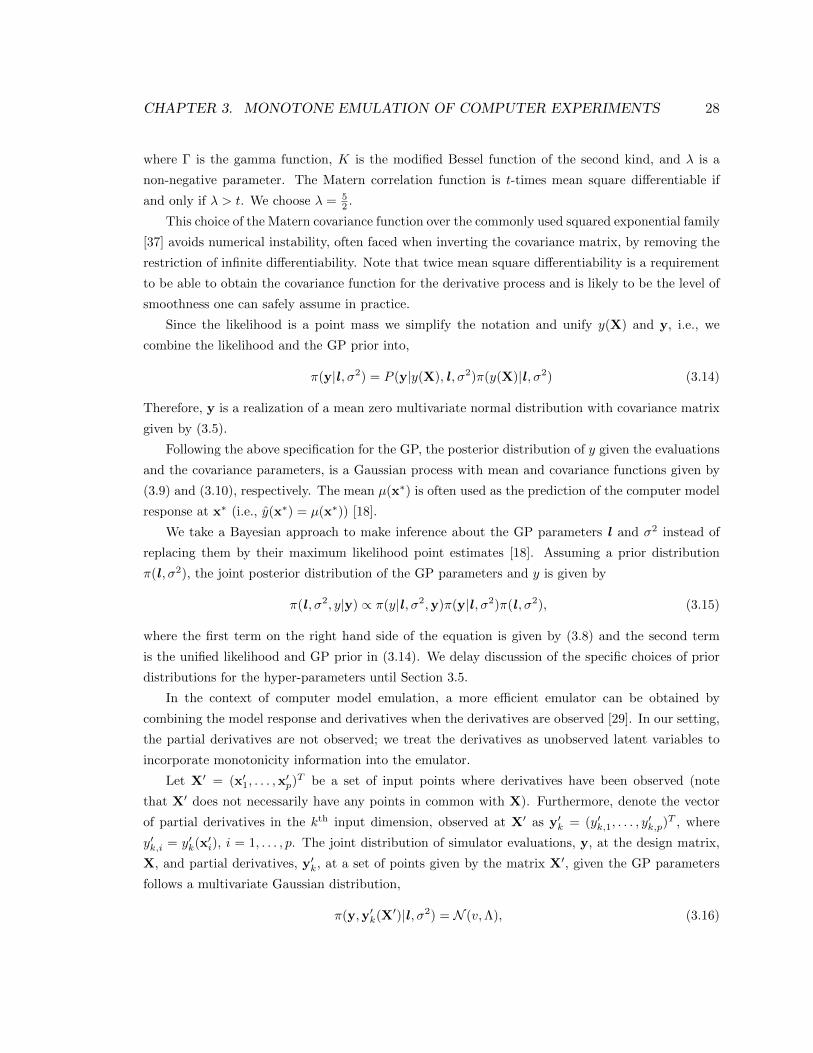
CHAPTER 3. MONOTONE EMULATION OF COMPUTER EXPERIMENTS 28
where Γ is the gamma function, K is the modified Bessel function of the second kind, and λ is a
non-negative parameter. The Matern correlation function is t-times mean square differentiable if
and only if λ > t. We choose λ = 52 .
This choice of the Matern covariance function over the commonly used squared exponential family
[37] avoids numerical instability, often faced when inverting the covariance matrix, by removing the
restriction of infinite differentiability. Note that twice mean square differentiability is a requirement
to be able to obtain the covariance function for the derivative process and is likely to be the level of
smoothness one can safely assume in practice.
Since the likelihood is a point mass we simplify the notation and unify y(X) and y, i.e., we
combine the likelihood and the GP prior into,
π(y|l , σ2) = P (y|y(X), l , σ2)π(y(X)|l , σ2) (3.14)
Therefore, y is a realization of a mean zero multivariate normal distribution with covariance matrix
given by (3.5).
Following the above specification for the GP, the posterior distribution of y given the evaluations
and the covariance parameters, is a Gaussian process with mean and covariance functions given by
(3.9) and (3.10), respectively. The mean µ(x∗) is often used as the prediction of the computer model
response at x∗ (i.e., y(x∗) = µ(x∗)) [18].
We take a Bayesian approach to make inference about the GP parameters l and σ2 instead of
replacing them by their maximum likelihood point estimates [18]. Assuming a prior distribution
π(l , σ2), the joint posterior distribution of the GP parameters and y is given by
π(l , σ2, y|y) ∝ π(y|l , σ2,y)π(y|l , σ2)π(l , σ2), (3.15)
where the first term on the right hand side of the equation is given by (3.8) and the second term
is the unified likelihood and GP prior in (3.14). We delay discussion of the specific choices of prior
distributions for the hyper-parameters until Section 3.5.
In the context of computer model emulation, a more efficient emulator can be obtained by
combining the model response and derivatives when the derivatives are observed [29]. In our setting,
the partial derivatives are not observed; we treat the derivatives as unobserved latent variables to
incorporate monotonicity information into the emulator.
Let X′ = (x′1, . . . ,x′p)T be a set of input points where derivatives have been observed (note
that X′ does not necessarily have any points in common with X). Furthermore, denote the vector
of partial derivatives in the kth input dimension, observed at X′ as y′k = (y′k,1, . . . , y′k,p)
T , where
y′k,i = y′k(x′i), i = 1, . . . , p. The joint distribution of simulator evaluations, y, at the design matrix,
X, and partial derivatives, y′k, at a set of points given by the matrix X′, given the GP parameters
follows a multivariate Gaussian distribution,
π(y,y′k(X′)|l , σ2) = N (v,Λ), (3.16)
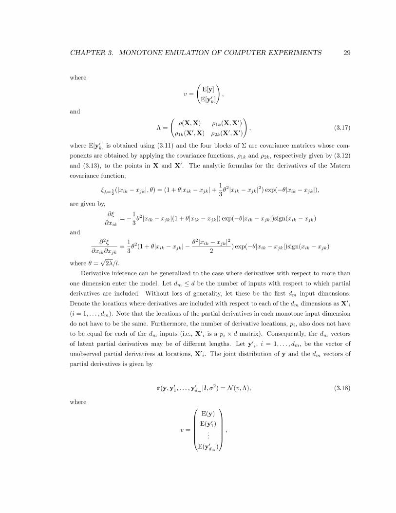
CHAPTER 3. MONOTONE EMULATION OF COMPUTER EXPERIMENTS 29
where
v =
(E[y]
E[y′k]
),
and
Λ =
(ρ(X,X) ρ1k(X,X′)
ρ1k(X′,X) ρ2k(X′,X′)
), (3.17)
where E[y′k] is obtained using (3.11) and the four blocks of Σ are covariance matrices whose com-
ponents are obtained by applying the covariance functions, ρ1k and ρ2k, respectively given by (3.12)
and (3.13), to the points in X and X′. The analytic formulas for the derivatives of the Matern
covariance function,
ξλ= 52(|xik − xjk|, θ) = (1 + θ|xik − xjk|+
1
3θ2|xik − xjk|2) exp(−θ|xik − xjk|),
are given by,
∂ξ
∂xik= −1
3θ2|xik − xjk|(1 + θ|xik − xjk|) exp(−θ|xik − xjk|)sign(xik − xjk)
and
∂2ξ
∂xik∂xjk=
1
3θ2(1 + θ|xik − xjk| −
θ2|xik − xjk|2
2) exp(−θ|xik − xjk|)sign(xik − xjk)
where θ =√
2λ/l.
Derivative inference can be generalized to the case where derivatives with respect to more than
one dimension enter the model. Let dm ≤ d be the number of inputs with respect to which partial
derivatives are included. Without loss of generality, let these be the first dm input dimensions.
Denote the locations where derivatives are included with respect to each of the dm dimensions as X′i
(i = 1, . . . , dm). Note that the locations of the partial derivatives in each monotone input dimension
do not have to be the same. Furthermore, the number of derivative locations, pi, also does not have
to be equal for each of the dm inputs (i.e., X′i is a pi × d matrix). Consequently, the dm vectors
of latent partial derivatives may be of different lengths. Let y′i, i = 1, . . . , dm, be the vector of
unobserved partial derivatives at locations, X′i. The joint distribution of y and the dm vectors of
partial derivatives is given by
π(y,y′1, . . . ,y′dm |l , σ
2) = N (v,Λ), (3.18)
where
v =
E(y)
E(y′1)...
E(y′dm)
,
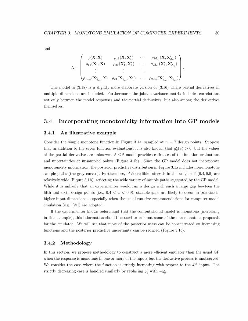
CHAPTER 3. MONOTONE EMULATION OF COMPUTER EXPERIMENTS 30
and
Λ =
ρ(X,X) ρ11(X,X′1) · · · ρ1dm(X,X′dm)
ρ11(X′1,X) ρ21(X′1,X′1) · · · ρ2dm(X′1,X
′dm
)...
.... . .
...
ρ1dm(X′dm ,X) ρ21(X′dm ,X′1) · · · ρ2dm(X′dm ,X
′dm
)
.
The model in (3.18) is a slightly more elaborate version of (3.16) where partial derivatives in
multiple dimensions are included. Furthermore, the joint covariance matrix includes correlations
not only between the model responses and the partial derivatives, but also among the derivatives
themselves.
3.4 Incorporating monotonicity information into GP models
3.4.1 An illustrative example
Consider the simple monotone function in Figure 3.1a, sampled at n = 7 design points. Suppose
that in addition to the seven function evaluations, it is also known that y′k(x) > 0, but the values
of the partial derivative are unknown. A GP model provides estimates of the function evaluations
and uncertainties at unsampled points (Figure 3.1b). Since the GP model does not incorporate
monotonicity information, the posterior predictive distribution in Figure 3.1a includes non-monotone
sample paths (the grey curves). Furthermore, 95% credible intervals in the range x ∈ (0.4, 0.9) are
relatively wide (Fiqure 3.1b), reflecting the wide variety of sample paths suggested by the GP model.
While it is unlikely that an experimenter would run a design with such a large gap bewteen the
fifth and sixth design points (i.e., 0.4 < x < 0.9), sizeable gaps are likely to occur in practice in
higher input dimensions - especially when the usual run-size recommendations for computer model
emulation (e.g., [21]) are adopted.
If the experimenter knows beforehand that the computational model is monotone (increasing
in this example), this information should be used to rule out some of the non-monotone proposals
for the emulator. We will see that most of the posterior mass can be concentrated on increasing
functions and the posterior predictive uncertainty can be reduced (Figure 3.1c).
3.4.2 Methodology
In this section, we propose methodology to construct a more efficient emulator than the usual GP
when the response is monotone in one or more of the inputs but the derivative process is unobserved.
We consider the case where the function is strictly increasing with respect to the kth input. The
strictly decreasing case is handled similarly by replacing y′k with −y′k.
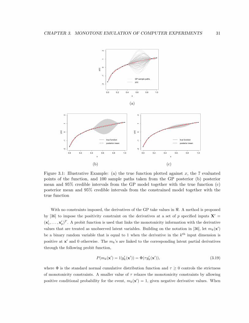
CHAPTER 3. MONOTONE EMULATION OF COMPUTER EXPERIMENTS 31
0.0 0.2 0.4 0.6 0.8 1.0
-2-1
01
2
x
y(x)
GP sample paths
y(x)
(a)
0.0 0.2 0.4 0.6 0.8 1.0
-2-1
01
2
x
y(x)
true function
posterior mean
(b)
0.0 0.2 0.4 0.6 0.8 1.0
-2-1
01
2
x
y(x)
true function
posterior mean
(c)
Figure 3.1: Illustrative Example: (a) the true function plotted against x, the 7 evaluatedpoints of the function, and 100 sample paths taken from the GP posterior (b) posteriormean and 95% credible intervals from the GP model together with the true function (c)posterior mean and 95% credible intervals from the constrained model together with thetrue function
With no constraints imposed, the derivatives of the GP take values in <. A method is proposed
by [36] to impose the positivity constraint on the derivatives at a set of p specified inputs X′ =
(x′1, . . . ,x′p)T . A probit function is used that links the monotonicity information with the derivative
values that are treated as unobserved latent variables. Building on the notation in [36], let mk(x′)
be a binary random variable that is equal to 1 when the derivative in the kth input dimension is
positive at x′ and 0 otherwise. The mk’s are linked to the corresponding latent partial derivatives
through the following probit function,
P (mk(x′) = 1|y′k(x′)) = Φ(τy′k(x′)), (3.19)
where Φ is the standard normal cumulative distribution function and τ ≥ 0 controls the strictness
of monotonicity constraints. A smaller value of τ relaxes the monotonicity constraints by allowing
positive conditional probability for the event, mk(x′) = 1, given negative derivative values. When
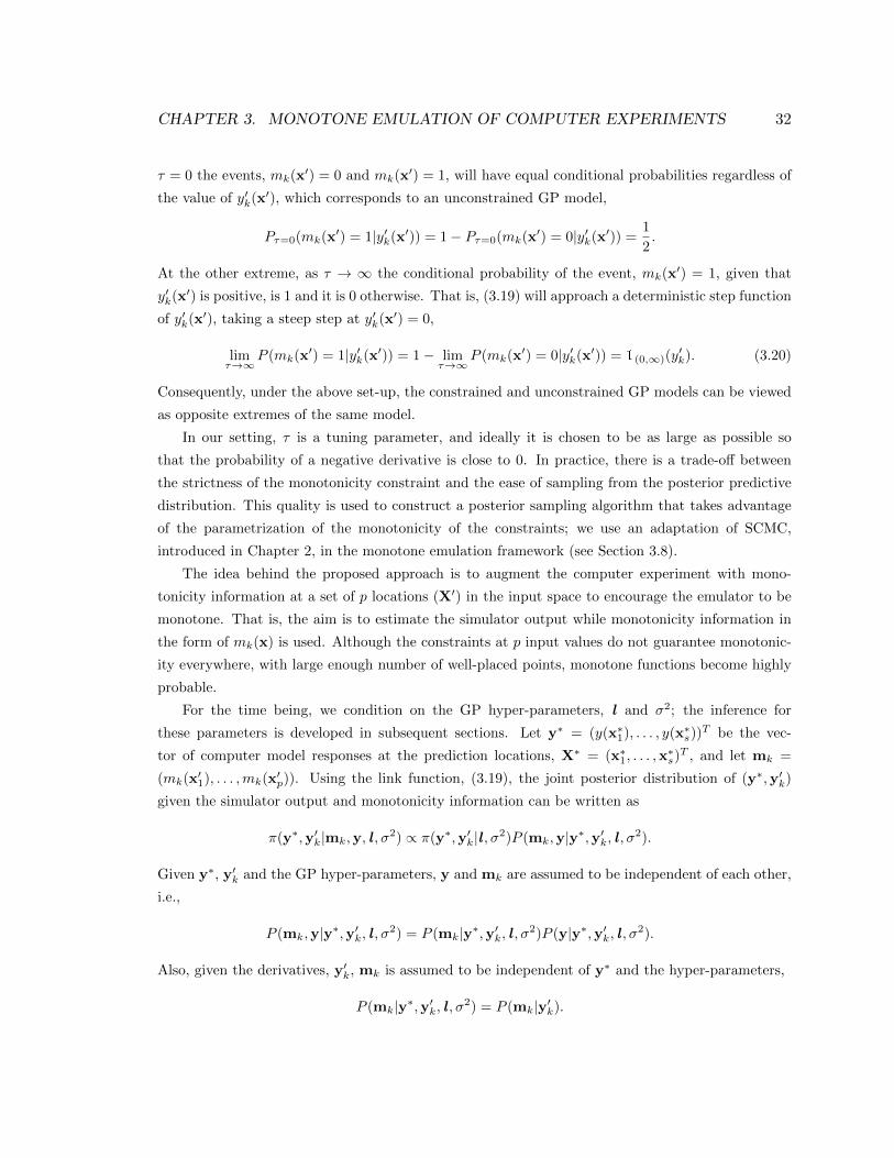
CHAPTER 3. MONOTONE EMULATION OF COMPUTER EXPERIMENTS 32
τ = 0 the events, mk(x′) = 0 and mk(x′) = 1, will have equal conditional probabilities regardless of
the value of y′k(x′), which corresponds to an unconstrained GP model,
Pτ=0(mk(x′) = 1|y′k(x′)) = 1− Pτ=0(mk(x′) = 0|y′k(x′)) =1
2.
At the other extreme, as τ → ∞ the conditional probability of the event, mk(x′) = 1, given that
y′k(x′) is positive, is 1 and it is 0 otherwise. That is, (3.19) will approach a deterministic step function
of y′k(x′), taking a steep step at y′k(x′) = 0,
limτ→∞
P (mk(x′) = 1|y′k(x′)) = 1− limτ→∞
P (mk(x′) = 0|y′k(x′)) = 1(0,∞)(y′k). (3.20)
Consequently, under the above set-up, the constrained and unconstrained GP models can be viewed
as opposite extremes of the same model.
In our setting, τ is a tuning parameter, and ideally it is chosen to be as large as possible so
that the probability of a negative derivative is close to 0. In practice, there is a trade-off between
the strictness of the monotonicity constraint and the ease of sampling from the posterior predictive
distribution. This quality is used to construct a posterior sampling algorithm that takes advantage
of the parametrization of the monotonicity of the constraints; we use an adaptation of SCMC,
introduced in Chapter 2, in the monotone emulation framework (see Section 3.8).
The idea behind the proposed approach is to augment the computer experiment with mono-
tonicity information at a set of p locations (X′) in the input space to encourage the emulator to be
monotone. That is, the aim is to estimate the simulator output while monotonicity information in
the form of mk(x) is used. Although the constraints at p input values do not guarantee monotonic-
ity everywhere, with large enough number of well-placed points, monotone functions become highly
probable.
For the time being, we condition on the GP hyper-parameters, l and σ2; the inference for
these parameters is developed in subsequent sections. Let y∗ = (y(x∗1), . . . , y(x∗s))T be the vec-
tor of computer model responses at the prediction locations, X∗ = (x∗1, . . . ,x∗s)T , and let mk =
(mk(x′1), . . . ,mk(x′p)). Using the link function, (3.19), the joint posterior distribution of (y∗,y′k)
given the simulator output and monotonicity information can be written as
π(y∗,y′k|mk,y, l , σ2) ∝ π(y∗,y′k|l , σ2)P (mk,y|y∗,y′k, l , σ2).
Given y∗, y′k and the GP hyper-parameters, y and mk are assumed to be independent of each other,
i.e.,
P (mk,y|y∗,y′k, l , σ2) = P (mk|y∗,y′k, l , σ2)P (y|y∗,y′k, l , σ2).
Also, given the derivatives, y′k, mk is assumed to be independent of y∗ and the hyper-parameters,
P (mk|y∗,y′k, l , σ2) = P (mk|y′k).
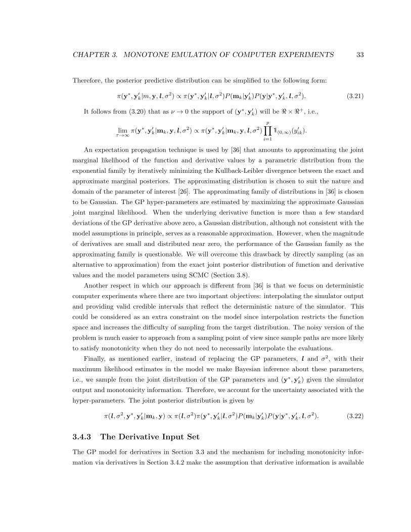
CHAPTER 3. MONOTONE EMULATION OF COMPUTER EXPERIMENTS 33
Therefore, the posterior predictive distribution can be simplified to the following form:
π(y∗,y′k|m,y, l , σ2) ∝ π(y∗,y′k|l , σ2)P (mk|y′k)P (y|y∗,y′k, l , σ2). (3.21)
It follows from (3.20) that as ν → 0 the support of (y∗,y′k) will be <× <+, i.e.,
limτ→∞
π(y∗,y′k|mk,y, l , σ2) ∝ π(y∗,y′k|mk,y, l , σ
2)
p∏i=1
1(0,∞)(y′ik).
An expectation propagation technique is used by [36] that amounts to approximating the joint
marginal likelihood of the function and derivative values by a parametric distribution from the
exponential family by iteratively minimizing the Kullback-Leibler divergence between the exact and
approximate marginal posteriors. The approximating distribution is chosen to suit the nature and
domain of the parameter of interest [26]. The approximating family of distributions in [36] is chosen
to be Gaussian. The GP hyper-parameters are estimated by maximizing the approximate Gaussian
joint marginal likelihood. When the underlying derivative function is more than a few standard
deviations of the GP derivative above zero, a Gaussian distribution, although not consistent with the
model assumptions in principle, serves as a reasonable approximation. However, when the magnitude
of derivatives are small and distributed near zero, the performance of the Gaussian family as the
approximating family is questionable. We will overcome this drawback by directly sampling (as an
alternative to approximation) from the exact joint posterior distribution of function and derivative
values and the model parameters using SCMC (Section 3.8).
Another respect in which our approach is different from [36] is that we focus on deterministic
computer experiments where there are two important objectives: interpolating the simulator output
and providing valid credible intervals that reflect the deterministic nature of the simulator. This
could be considered as an extra constraint on the model since interpolation restricts the function
space and increases the difficulty of sampling from the target distribution. The noisy version of the
problem is much easier to approach from a sampling point of view since sample paths are more likely
to satisfy monotonicity when they do not need to necessarily interpolate the evaluations.
Finally, as mentioned earlier, instead of replacing the GP parameters, l and σ2, with their
maximum likelihood estimates in the model we make Bayesian inference about these parameters,
i.e., we sample from the joint distribution of the GP parameters and (y∗,y′k) given the simulator
output and monotonicity information. Therefore, we account for the uncertainty associated with the
hyper-parameters. The joint posterior distribution is given by
π(l , σ2,y∗,y′k|mk,y) ∝ π(l , σ2)π(y∗,y′k|l , σ2)P (mk|y′k)P (y|y∗,y′k, l , σ2). (3.22)
3.4.3 The Derivative Input Set
The GP model for derivatives in Section 3.3 and the mechanism for including monotonicity infor-
mation via derivatives in Section 3.4.2 make the assumption that derivative information is available
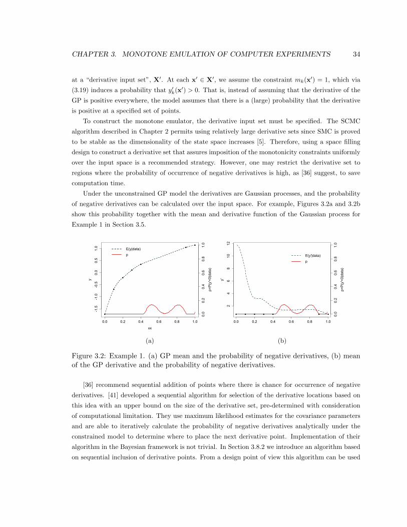
CHAPTER 3. MONOTONE EMULATION OF COMPUTER EXPERIMENTS 34
at a “derivative input set”, X′. At each x′ ∈ X′, we assume the constraint mk(x′) = 1, which via
(3.19) induces a probability that y′k(x′) > 0. That is, instead of assuming that the derivative of the
GP is positive everywhere, the model assumes that there is a (large) probability that the derivative
is positive at a specified set of points.
To construct the monotone emulator, the derivative input set must be specified. The SCMC
algorithm described in Chapter 2 permits using relatively large derivative sets since SMC is proved
to be stable as the dimensionality of the state space increases [5]. Therefore, using a space filling
design to construct a derivative set that assures imposition of the monotonicity constraints uniformly
over the input space is a recommended strategy. However, one may restrict the derivative set to
regions where the probability of occurrence of negative derivatives is high, as [36] suggest, to save
computation time.
Under the unconstrained GP model the derivatives are Gaussian processes, and the probability
of negative derivatives can be calculated over the input space. For example, Figures 3.2a and 3.2b
show this probability together with the mean and derivative function of the Gaussian process for
Example 1 in Section 3.5.
0.0 0.2 0.4 0.6 0.8 1.0
-1.5
-1.0
-0.5
0.0
0.5
1.0
xx
y
E(y|data)
p
0.0
0.2
0.4
0.6
0.8
1.0
p=P(y'<0|data)
(a)
0.0 0.2 0.4 0.6 0.8 1.0
24
68
1012
y'
E(y'|data)
p
0.0
0.2
0.4
0.6
0.8
1.0
p=P(y'<0|data)
(b)
Figure 3.2: Example 1. (a) GP mean and the probability of negative derivatives, (b) meanof the GP derivative and the probability of negative derivatives.
[36] recommend sequential addition of points where there is chance for occurrence of negative
derivatives. [41] developed a sequential algorithm for selection of the derivative locations based on
this idea with an upper bound on the size of the derivative set, pre-determined with consideration
of computational limitation. They use maximum likelihood estimates for the covariance parameters
and are able to iteratively calculate the probability of negative derivatives analytically under the
constrained model to determine where to place the next derivative point. Implementation of their
algorithm in the Bayesian framework is not trivial. In Section 3.8.2 we introduce an algorithm based
on sequential inclusion of derivative points. From a design point of view this algorithm can be used
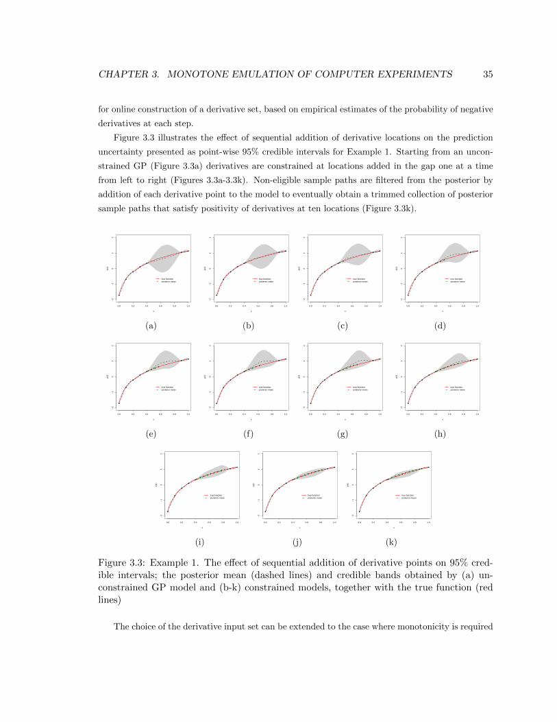
CHAPTER 3. MONOTONE EMULATION OF COMPUTER EXPERIMENTS 35
for online construction of a derivative set, based on empirical estimates of the probability of negative
derivatives at each step.
Figure 3.3 illustrates the effect of sequential addition of derivative locations on the prediction
uncertainty presented as point-wise 95% credible intervals for Example 1. Starting from an uncon-
strained GP (Figure 3.3a) derivatives are constrained at locations added in the gap one at a time
from left to right (Figures 3.3a-3.3k). Non-eligible sample paths are filtered from the posterior by
addition of each derivative point to the model to eventually obtain a trimmed collection of posterior
sample paths that satisfy positivity of derivatives at ten locations (Figure 3.3k).
●
●
●
●
●
●●
0.0 0.2 0.4 0.6 0.8 1.0
−2
−1
01
2
x
y(x)
●
●
●
●
●
●●
true functionposterior mean
(a)
●
●
●
●
●
●●
0.0 0.2 0.4 0.6 0.8 1.0
−2
−1
01
2
x
y(x)
●
●
●
●
●
●●
true functionposterior mean
(b)
●
●
●
●
●
●●
0.0 0.2 0.4 0.6 0.8 1.0−
2−
10
12
x
y(x)
●
●
●
●
●
●●
true functionposterior mean
(c)
●
●
●
●
●
●●
0.0 0.2 0.4 0.6 0.8 1.0
−2
−1
01
2
x
y(x)
●
●
●
●
●
●●
true functionposterior mean
(d)
●
●
●
●
●
●●
0.0 0.2 0.4 0.6 0.8 1.0
−2
−1
01
2
x
y(x)
●
●
●
●
●
●●
true functionposterior mean
(e)
●
●
●
●
●
●●
0.0 0.2 0.4 0.6 0.8 1.0
−2
−1
01
2
x
y(x)
●
●
●
●
●
●●
true functionposterior mean
(f)
●
●
●
●
●
●●
0.0 0.2 0.4 0.6 0.8 1.0
−2
−1
01
2
x
y(x)
●
●
●
●
●
●●
true functionposterior mean
(g)
●
●
●
●
●
●●
0.0 0.2 0.4 0.6 0.8 1.0
−2
−1
01
2
x
y(x)
●
●
●
●
●
●●
true functionposterior mean
(h)
●
●
●
●
●
●●
0.0 0.2 0.4 0.6 0.8 1.0
−2
−1
01
2
x
y(x)
●
●
●
●
●
●●
true functionposterior mean
(i)
●
●
●
●
●
●●
0.0 0.2 0.4 0.6 0.8 1.0
−2
−1
01
2
x
y(x)
●
●
●
●
●
●●
true functionposterior mean
(j)
●
●
●
●
●
●●
0.0 0.2 0.4 0.6 0.8 1.0
−2
−1
01
2
x
y(x)
●
●
●
●
●
●●
true functionposterior mean
(k)
Figure 3.3: Example 1. The effect of sequential addition of derivative points on 95% cred-ible intervals; the posterior mean (dashed lines) and credible bands obtained by (a) un-constrained GP model and (b-k) constrained models, together with the true function (redlines)
The choice of the derivative input set can be extended to the case where monotonicity is required
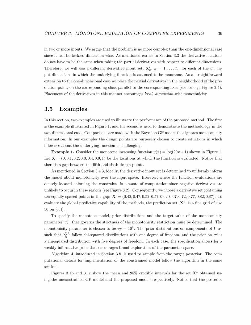
CHAPTER 3. MONOTONE EMULATION OF COMPUTER EXPERIMENTS 36
in two or more inputs. We argue that the problem is no more complex than the one-dimensional case
since it can be tackled dimension-wise. As mentioned earlier in Section 3.3 the derivative locations
do not have to be the same when taking the partial derivatives with respect to different dimensions.
Therefore, we will use a different derivative input set, X′k, k = 1, . . . , dm for each of the dm in-
put dimensions in which the underlying function is assumed to be monotone. As a straightforward
extension to the one-dimensional case we place the partial derivatives in the neighborhood of the pre-
diction point, on the corresponding slice, parallel to the corresponding axes (see for e.g. Figure 3.4).
Placement of the derivatives in this manner encourages local, dimension-wise monotonicity.
3.5 Examples
In this section, two examples are used to illustrate the performance of the proposed method. The first
is the example illustrated in Figure 1, and the second is used to demonstrate the methodology in the
two-dimensional case. Comparisons are made with the Bayesian GP model that ignores monotonicity
information. In our examples the design points are purposely chosen to create situations in which
inference about the underlying function is challenging.
Example 1. Consider the monotone increasing function y(x) = log(20x+ 1) shown in Figure 1.
Let X = (0, 0.1, 0.2, 0.3, 0.4, 0.9, 1) be the locations at which the function is evaluated. Notice that
there is a gap between the fifth and sixth design points.
As mentioned in Section 3.4.3, ideally, the derivative input set is determined to uniformly inform
the model about monotonicity over the input space. However, where the function evaluations are
densely located enforcing the constraints is a waste of computation since negative derivatives are
unlikely to occur in these regions (see Figure 3.2). Consequently, we choose a derivative set containing
ten equally spaced points in the gap: X′ = (0.42, 0.47, 0.52, 0.57, 0.62, 0.67, 0.72, 0.77, 0.82, 0.87). To
evaluate the global predictive capability of the methods, the prediction set, X∗, is a fine grid of size
50 on [0, 1].
To specify the monotone model, prior distributions and the target value of the monotonicity
parameter, τT , that governs the strictness of the monotonicity restriction must be determined. The
monotonicity parameter is chosen to be τT = 106. The prior distributions on components of l are
such that√2λlk
follow chi-squared distributions with one degree of freedom, and the prior on σ2 is
a chi-squared distribution with five degrees of freedom. In each case, the specification allows for a
weakly informative prior that encourages broad exploration of the parameter space.
Algorithm 4, introduced in Section 3.8, is used to sample from the target posterior. The com-
putational details for implementation of the constrained model follow the algorithm in the same
section.
Figures 3.1b and 3.1c show the mean and 95% credible intervals for the set X∗ obtained us-
ing the unconstrained GP model and the proposed model, respectively. Notice that the posterior
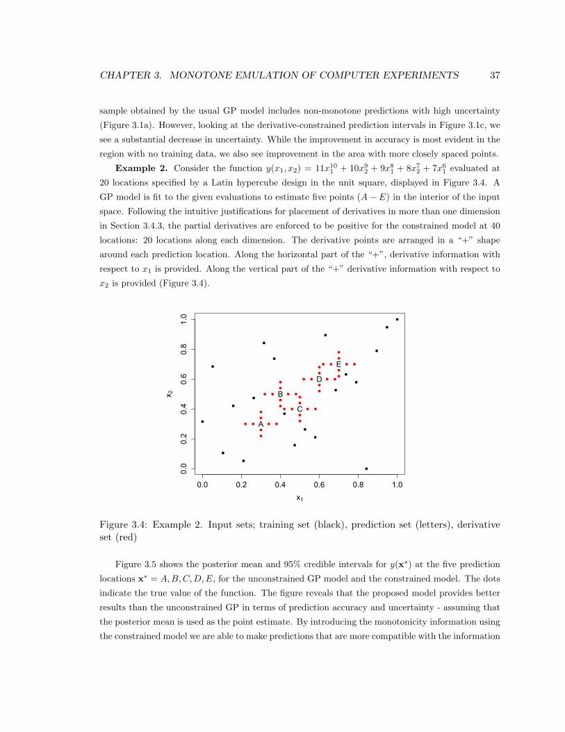
CHAPTER 3. MONOTONE EMULATION OF COMPUTER EXPERIMENTS 37
sample obtained by the usual GP model includes non-monotone predictions with high uncertainty
(Figure 3.1a). However, looking at the derivative-constrained prediction intervals in Figure 3.1c, we
see a substantial decrease in uncertainty. While the improvement in accuracy is most evident in the
region with no training data, we also see improvement in the area with more closely spaced points.
Example 2. Consider the function y(x1, x2) = 11x101 + 10x92 + 9x81 + 8x72 + 7x61 evaluated at
20 locations specified by a Latin hypercube design in the unit square, displayed in Figure 3.4. A
GP model is fit to the given evaluations to estimate five points (A− E) in the interior of the input
space. Following the intuitive justifications for placement of derivatives in more than one dimension
in Section 3.4.3, the partial derivatives are enforced to be positive for the constrained model at 40
locations: 20 locations along each dimension. The derivative points are arranged in a “+” shape
around each prediction location. Along the horizontal part of the “+”, derivative information with
respect to x1 is provided. Along the vertical part of the “+” derivative information with respect to
x2 is provided (Figure 3.4).
0.0 0.2 0.4 0.6 0.8 1.0
0.0
0.2
0.4
0.6
0.8
1.0
x1
x 2
A
B
C
D
E
Figure 3.4: Example 2. Input sets; training set (black), prediction set (letters), derivativeset (red)
Figure 3.5 shows the posterior mean and 95% credible intervals for y(x∗) at the five prediction
locations x∗ = A,B,C,D,E, for the unconstrained GP model and the constrained model. The dots
indicate the true value of the function. The figure reveals that the proposed model provides better
results than the unconstrained GP in terms of prediction accuracy and uncertainty - assuming that
the posterior mean is used as the point estimate. By introducing the monotonicity information using
the constrained model we are able to make predictions that are more compatible with the information
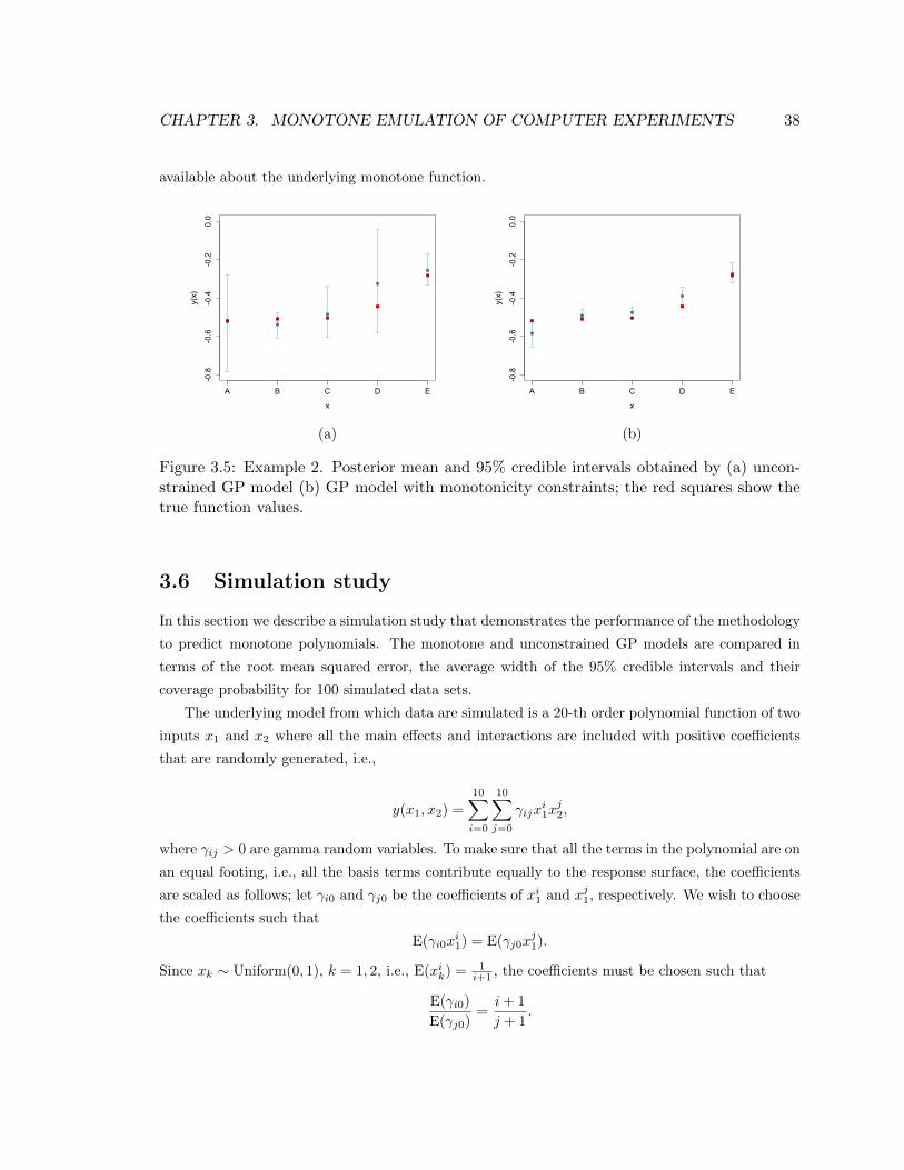
CHAPTER 3. MONOTONE EMULATION OF COMPUTER EXPERIMENTS 38
available about the underlying monotone function.
-0.8
-0.6
-0.4
-0.2
0.0
x
y(x)
A B C D E
(a)
-0.8
-0.6
-0.4
-0.2
0.0
x
y(x)
A B C D E
(b)
Figure 3.5: Example 2. Posterior mean and 95% credible intervals obtained by (a) uncon-strained GP model (b) GP model with monotonicity constraints; the red squares show thetrue function values.
3.6 Simulation study
In this section we describe a simulation study that demonstrates the performance of the methodology
to predict monotone polynomials. The monotone and unconstrained GP models are compared in
terms of the root mean squared error, the average width of the 95% credible intervals and their
coverage probability for 100 simulated data sets.
The underlying model from which data are simulated is a 20-th order polynomial function of two
inputs x1 and x2 where all the main effects and interactions are included with positive coefficients
that are randomly generated, i.e.,
y(x1, x2) =
10∑i=0
10∑j=0
γijxi1xj2,
where γij > 0 are gamma random variables. To make sure that all the terms in the polynomial are on
an equal footing, i.e., all the basis terms contribute equally to the response surface, the coefficients
are scaled as follows; let γi0 and γj0 be the coefficients of xi1 and xj1, respectively. We wish to choose
the coefficients such that
E(γi0xi1) = E(γj0x
j1).
Since xk ∼ Uniform(0, 1), k = 1, 2, i.e., E(xik) = 1i+1 , the coefficients must be chosen such that
E(γi0)
E(γj0)=i+ 1
j + 1.
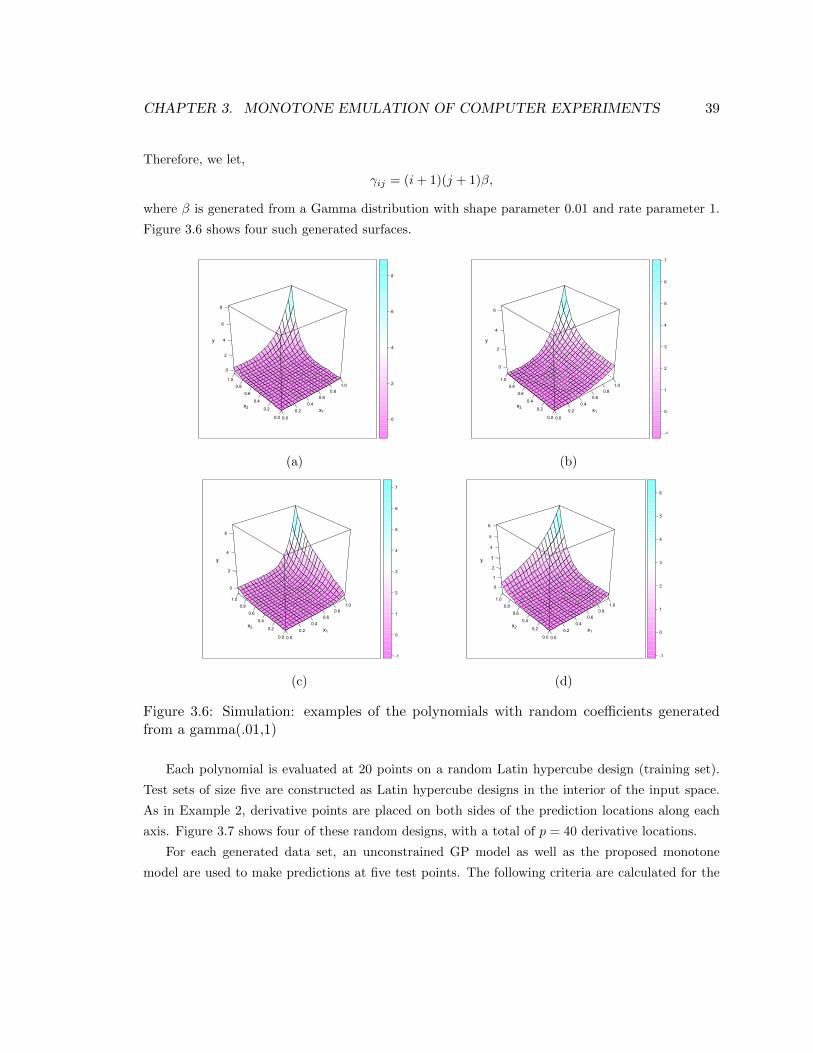
CHAPTER 3. MONOTONE EMULATION OF COMPUTER EXPERIMENTS 39
Therefore, we let,
γij = (i+ 1)(j + 1)β,
where β is generated from a Gamma distribution with shape parameter 0.01 and rate parameter 1.
Figure 3.6 shows four such generated surfaces.
0.0
0.2
0.4
0.6
0.81.0
0.0
0.2
0.4
0.6
0.8
1.0
0
2
4
6
8
x1x2
y
0
2
4
6
8
(a)
0.0
0.2
0.4
0.6
0.81.0
0.0
0.2
0.4
0.6
0.8
1.0
0
2
4
6
x1x2
y
-1
0
1
2
3
4
5
6
7
(b)
0.0
0.2
0.4
0.6
0.81.0
0.0
0.2
0.4
0.6
0.8
1.0
0
2
4
6
x1x2
y
-1
0
1
2
3
4
5
6
7
(c)
0.0
0.2
0.4
0.6
0.81.0
0.0
0.2
0.4
0.6
0.8
1.0
0
1
2
3
4
5
6
x1x2
y
-1
0
1
2
3
4
5
6
(d)
Figure 3.6: Simulation: examples of the polynomials with random coefficients generatedfrom a gamma(.01,1)
Each polynomial is evaluated at 20 points on a random Latin hypercube design (training set).
Test sets of size five are constructed as Latin hypercube designs in the interior of the input space.
As in Example 2, derivative points are placed on both sides of the prediction locations along each
axis. Figure 3.7 shows four of these random designs, with a total of p = 40 derivative locations.
For each generated data set, an unconstrained GP model as well as the proposed monotone
model are used to make predictions at five test points. The following criteria are calculated for the
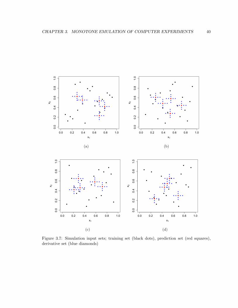
CHAPTER 3. MONOTONE EMULATION OF COMPUTER EXPERIMENTS 40
0.0 0.2 0.4 0.6 0.8 1.0
0.0
0.2
0.4
0.6
0.8
1.0
x1
x 2
(a)
0.0 0.2 0.4 0.6 0.8 1.00.0
0.2
0.4
0.6
0.8
1.0
x1
x 2
(b)
0.0 0.2 0.4 0.6 0.8 1.0
0.0
0.2
0.4
0.6
0.8
1.0
x1
x 2
(c)
0.0 0.2 0.4 0.6 0.8 1.0
0.0
0.2
0.4
0.6
0.8
1.0
x1
x 2
(d)
Figure 3.7: Simulation input sets; training set (black dots), prediction set (red squares),derivative set (blue diamonds)
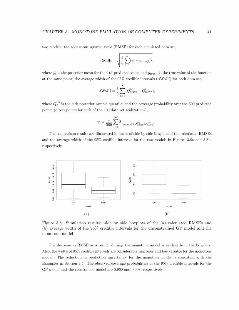
CHAPTER 3. MONOTONE EMULATION OF COMPUTER EXPERIMENTS 41
two models: the root mean squared error (RMSE) for each simulated data set,
RMSE =
√√√√1
5
5∑i=1
(yi − ytrue,i)2,
where yi is the posterior mean for the i-th predicted value and ytrue,i is the true value of the function
at the same point; the average width of the 95% credible intervals (AWoCI) for each data set,
AWoCI =1
5
5∑i=1
(Q(i)0.975 −Q
(i)0.025),
where Q(i)c is the c-th posterior sample quantile; and the coverage probability over the 500 predicted
points (5 test points for each of the 100 data set realizations),
cp =1
500
500∑i=1
δ{ytrue,i∈(Q(i)0.025,Q
(i)0.975)}
.
The comparison results are illustrated in forms of side by side boxplots of the calculated RMSEs
and the average width of the 95% credible intervals for the two models in Figures 3.8a and 3.8b,
respectively.
GP mon
0.00
0.05
0.10
0.15
0.20
model
RMSE
(a)
GP mon
0.2
0.4
0.6
0.8
model
AWoCI
(b)
Figure 3.8: Simulation results: side by side boxplots of the (a) calculated RMSEs and(b) average width of the 95% credible intervals for the unconstrained GP model and themonotone model
The decrease in RMSE as a result of using the monotone model is evident from the boxplots.
Also, the width of 95% credible intervals are considerably narrower and less variable for the monotone
model. The reduction in prediction uncertainty for the monotone model is consistent with the
Examples in Section 3.5. The observed coverage probabilities of the 95% credible intervals for the
GP model and the constrained model are 0.960 and 0.908, respectively.
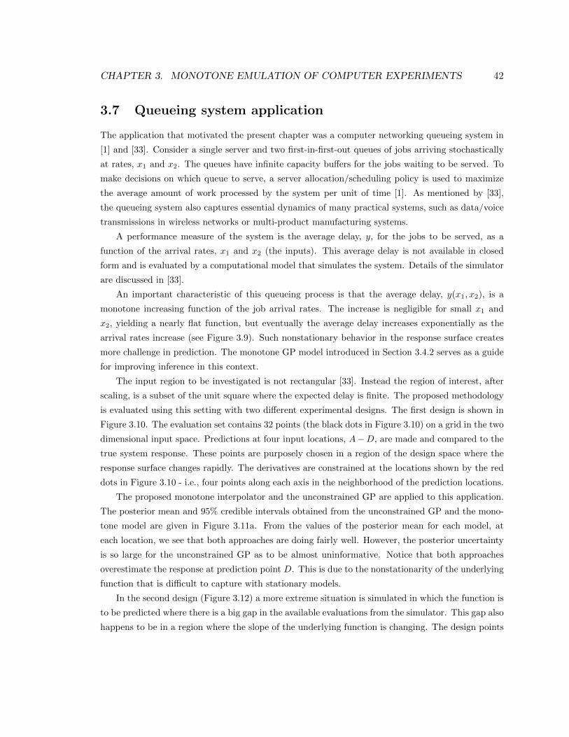
CHAPTER 3. MONOTONE EMULATION OF COMPUTER EXPERIMENTS 42
3.7 Queueing system application
The application that motivated the present chapter was a computer networking queueing system in
[1] and [33]. Consider a single server and two first-in-first-out queues of jobs arriving stochastically
at rates, x1 and x2. The queues have infinite capacity buffers for the jobs waiting to be served. To
make decisions on which queue to serve, a server allocation/scheduling policy is used to maximize
the average amount of work processed by the system per unit of time [1]. As mentioned by [33],
the queueing system also captures essential dynamics of many practical systems, such as data/voice
transmissions in wireless networks or multi-product manufacturing systems.
A performance measure of the system is the average delay, y, for the jobs to be served, as a
function of the arrival rates, x1 and x2 (the inputs). This average delay is not available in closed
form and is evaluated by a computational model that simulates the system. Details of the simulator
are discussed in [33].
An important characteristic of this queueing process is that the average delay, y(x1, x2), is a
monotone increasing function of the job arrival rates. The increase is negligible for small x1 and
x2, yielding a nearly flat function, but eventually the average delay increases exponentially as the
arrival rates increase (see Figure 3.9). Such nonstationary behavior in the response surface creates
more challenge in prediction. The monotone GP model introduced in Section 3.4.2 serves as a guide
for improving inference in this context.
The input region to be investigated is not rectangular [33]. Instead the region of interest, after
scaling, is a subset of the unit square where the expected delay is finite. The proposed methodology
is evaluated using this setting with two different experimental designs. The first design is shown in
Figure 3.10. The evaluation set contains 32 points (the black dots in Figure 3.10) on a grid in the two
dimensional input space. Predictions at four input locations, A−D, are made and compared to the
true system response. These points are purposely chosen in a region of the design space where the
response surface changes rapidly. The derivatives are constrained at the locations shown by the red
dots in Figure 3.10 - i.e., four points along each axis in the neighborhood of the prediction locations.
The proposed monotone interpolator and the unconstrained GP are applied to this application.
The posterior mean and 95% credible intervals obtained from the unconstrained GP and the mono-
tone model are given in Figure 3.11a. From the values of the posterior mean for each model, at
each location, we see that both approaches are doing fairly well. However, the posterior uncertainty
is so large for the unconstrained GP as to be almost uninformative. Notice that both approaches
overestimate the response at prediction point D. This is due to the nonstationarity of the underlying
function that is difficult to capture with stationary models.
In the second design (Figure 3.12) a more extreme situation is simulated in which the function is
to be predicted where there is a big gap in the available evaluations from the simulator. This gap also
happens to be in a region where the slope of the underlying function is changing. The design points
CHAPTER 3. MONOTONE EMULATION OF COMPUTER EXPERIMENTS 43
24
68
1012
14
2
4
68
1012
14
10
20
30
40
x1x2
y(x1, x2)
0
5
10
15
20
25
30
35
40
Figure 3.9: queueing application: the average delay as a function of the two job arrival rates
are shown in Figure 3.12, as well as the derivative-constrained points and the test points A−D. The
contours of the average delay are also plotted to illustrate the rapid change in the response surface.
The posterior mean and 95% credible intervals obtained from the unconstrained GP and the
monotone model for this setting are given in Figure 3.13. The improvement in terms of uncertainty
reduction for the constrained GP is also evident for this design. However, the posterior uncertainty
for prediction point D is underestimated and the 95% credible interval misses the true value of the
function. Again, nonstationarity of the responce surface as well as sparcity of the evaluations in this
area are factors contributiong to the poor prediction results given by the two models. In terms of
MSE, the monotone GP is doing relatively well (the MSE is about 0.3 for unconstrained model and
about 0.1 for the constrained model).
Making predictions for this queueing application is challenging for both models. As mentioned
before, the response surface (Figure 3.9) is flat for much of the input space and increases rapidly near
the boundary of the input region. This is not the behavior of a simulator that can be captured by a
stationary model. However, overall, taking monotonicity into account helped reduce the predictive
MSE and also the uncertainty in the predictions.
3.8 SCMC for Monotone Emulation
In this section we outline the adaptations of the SCMC algorithm from Chapter 2 to sample the
unobserved function values, y∗, derivative values, y′, and covariance parameter values, l and σ2, from
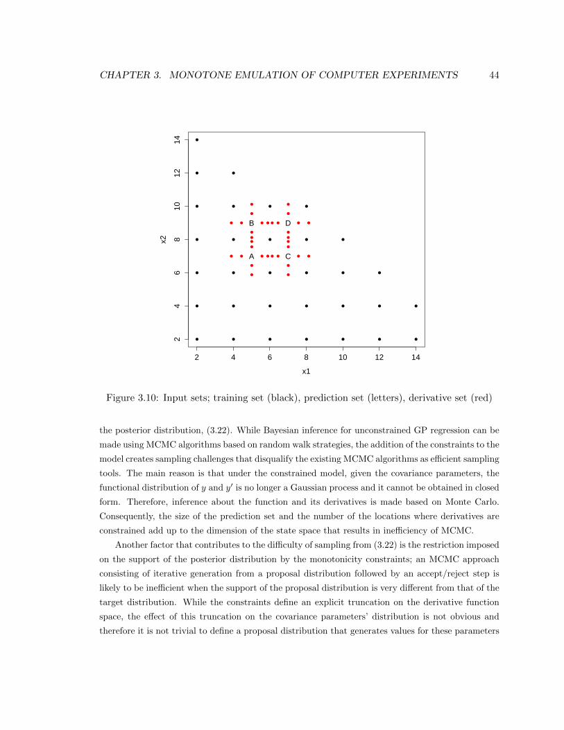
CHAPTER 3. MONOTONE EMULATION OF COMPUTER EXPERIMENTS 44
●
●
●
●
●
●
●
●
●
●
●
●
●
●
●
●
●
●
●
●
●
●
●
●
●
●
●
●
●
●
●
●
2 4 6 8 10 12 14
24
68
1012
14
x1
x2
A
B
C
D
●●●●●●●●
●●●●●●●●
●●●●●●●●
●●●●●●●●
● ● ● ●
● ● ● ●
● ● ● ●
● ● ● ●
●
●
●
●●
●
●
●
●
●
●
●●
●
●
●
Figure 3.10: Input sets; training set (black), prediction set (letters), derivative set (red)
the posterior distribution, (3.22). While Bayesian inference for unconstrained GP regression can be
made using MCMC algorithms based on random walk strategies, the addition of the constraints to the
model creates sampling challenges that disqualify the existing MCMC algorithms as efficient sampling
tools. The main reason is that under the constrained model, given the covariance parameters, the
functional distribution of y and y′ is no longer a Gaussian process and it cannot be obtained in closed
form. Therefore, inference about the function and its derivatives is made based on Monte Carlo.
Consequently, the size of the prediction set and the number of the locations where derivatives are
constrained add up to the dimension of the state space that results in inefficiency of MCMC.
Another factor that contributes to the difficulty of sampling from (3.22) is the restriction imposed
on the support of the posterior distribution by the monotonicity constraints; an MCMC approach
consisting of iterative generation from a proposal distribution followed by an accept/reject step is
likely to be inefficient when the support of the proposal distribution is very different from that of the
target distribution. While the constraints define an explicit truncation on the derivative function
space, the effect of this truncation on the covariance parameters’ distribution is not obvious and
therefore it is not trivial to define a proposal distribution that generates values for these parameters
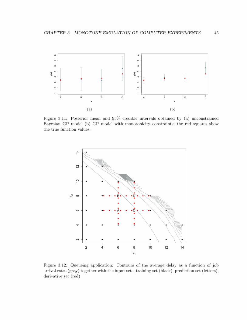
CHAPTER 3. MONOTONE EMULATION OF COMPUTER EXPERIMENTS 45
12
34
56
78
x
y(x)
A B C D
(a)
12
34
56
78
x
y(x)
A B C D
(b)
Figure 3.11: Posterior mean and 95% credible intervals obtained by (a) unconstrainedBayesian GP model (b) GP model with monotonicity constraints; the red squares showthe true function values.
2 4 6 8 10 12 14
24
68
1012
14
x1
x 2
A
B
C
D
Figure 3.12: Queueing application: Contours of the average delay as a function of jobarrival rates (gray) together with the input sets; training set (black), prediction set (letters),derivative set (red)
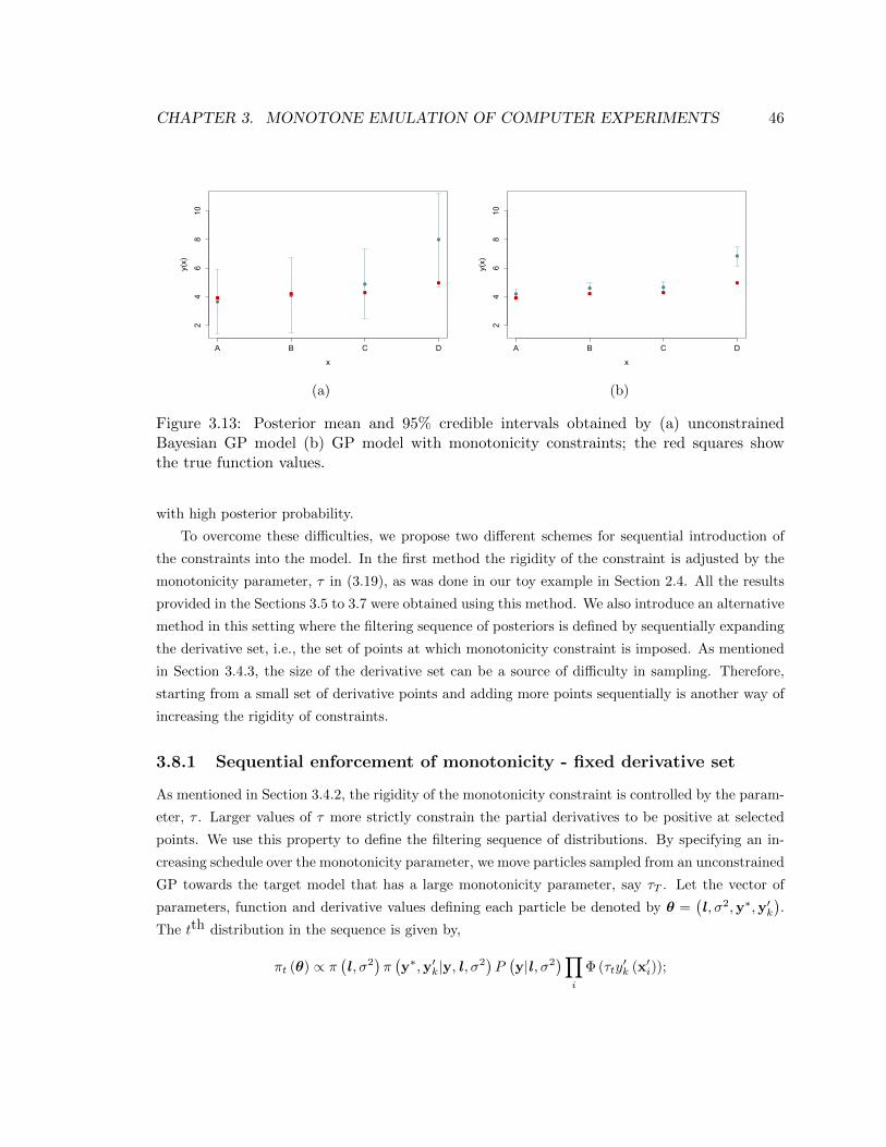
CHAPTER 3. MONOTONE EMULATION OF COMPUTER EXPERIMENTS 46
24
68
10
x
y(x)
A B C D
(a)
24
68
10
x
y(x)
A B C D
(b)
Figure 3.13: Posterior mean and 95% credible intervals obtained by (a) unconstrainedBayesian GP model (b) GP model with monotonicity constraints; the red squares showthe true function values.
with high posterior probability.
To overcome these difficulties, we propose two different schemes for sequential introduction of
the constraints into the model. In the first method the rigidity of the constraint is adjusted by the
monotonicity parameter, τ in (3.19), as was done in our toy example in Section 2.4. All the results
provided in the Sections 3.5 to 3.7 were obtained using this method. We also introduce an alternative
method in this setting where the filtering sequence of posteriors is defined by sequentially expanding
the derivative set, i.e., the set of points at which monotonicity constraint is imposed. As mentioned
in Section 3.4.3, the size of the derivative set can be a source of difficulty in sampling. Therefore,
starting from a small set of derivative points and adding more points sequentially is another way of
increasing the rigidity of constraints.
3.8.1 Sequential enforcement of monotonicity - fixed derivative set
As mentioned in Section 3.4.2, the rigidity of the monotonicity constraint is controlled by the param-
eter, τ . Larger values of τ more strictly constrain the partial derivatives to be positive at selected
points. We use this property to define the filtering sequence of distributions. By specifying an in-
creasing schedule over the monotonicity parameter, we move particles sampled from an unconstrained
GP towards the target model that has a large monotonicity parameter, say τT . Let the vector of
parameters, function and derivative values defining each particle be denoted by θ =(l , σ2,y∗,y′k
).
The tth distribution in the sequence is given by,
πt (θ) ∝ π(l , σ2
)π(y∗,y′k|y, l , σ2
)P(y|l , σ2
)∏i
Φ (τty′k (x′i));
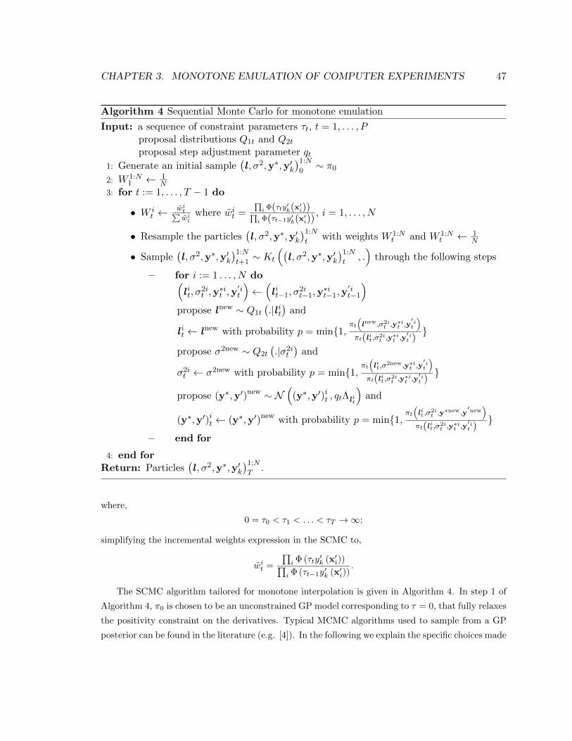
CHAPTER 3. MONOTONE EMULATION OF COMPUTER EXPERIMENTS 47
Algorithm 4 Sequential Monte Carlo for monotone emulation
Input: a sequence of constraint parameters τt, t = 1, . . . , Pproposal distributions Q1t and Q2t
proposal step adjustment parameter qt1: Generate an initial sample
(l , σ2,y∗,y′k
)1:N
0∼ π0
2: W 1:N1 ← 1
N3: for t := 1, . . . , T − 1 do
• W it ←
wit∑wi
twhere wit =
∏i Φ(τty′k(x′i))∏
i Φ(τt−1y′k(x′i)), i = 1, . . . , N
• Resample the particles(l , σ2,y∗,y′k
)1:N
twith weights W 1:N
t and W 1:Nt ← 1
N
• Sample(l , σ2,y∗,y′k
)1:N
t+1∼ Kt
((l , σ2,y∗,y′k
)1:N
t, .)
through the following steps
– for i := 1 . . . , N do(l it, σ
2it ,y
∗it ,y
′it
)←(l it−1, σ
2it−1,y
∗it−1,y
′it−1
)propose lnew ∼ Q1t
(.|l it)
and
l it ← lnew with probability p = min{1,πt(lnew,σ2i
t ,y∗it ,y
′it
)πt(l it,σ2i
t ,y∗it ,y
′it )}
propose σ2new ∼ Q2t
(.|σ2i
t
)and
σ2it ← σ2new with probability p = min{1,
πt(l it,σ
2new,y∗it ,y′it
)πt(l it,σ2i
t ,y∗it ,y
′it )}
propose (y∗,y′)new ∼ N(
(y∗,y′)it , qtΛl it
)and
(y∗,y′)it ← (y∗,y′)new with probability p = min{1,πt(l it,σ
2it ,y
∗new,y′new
)πt(l it,σ2i
t ,y∗it ,y
′it )
}
– end for
4: end forReturn: Particles
(l , σ2,y∗,y′k
)1:N
T.
where,
0 = τ0 < τ1 < . . . < τT →∞;
simplifying the incremental weights expression in the SCMC to,
wit =
∏i Φ (τty
′k (x′i))∏
i Φ (τt−1y′k (x′i)).
The SCMC algorithm tailored for monotone interpolation is given in Algorithm 4. In step 1 of
Algorithm 4, π0 is chosen to be an unconstrained GP model corresponding to τ = 0, that fully relaxes
the positivity constraint on the derivatives. Typical MCMC algorithms used to sample from a GP
posterior can be found in the literature (e.g. [4]). In the following we explain the specific choices made
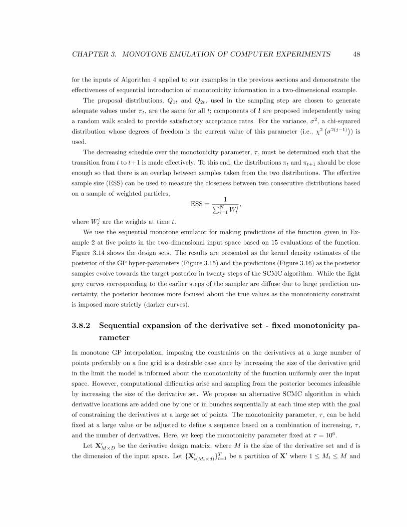
CHAPTER 3. MONOTONE EMULATION OF COMPUTER EXPERIMENTS 48
for the inputs of Algorithm 4 applied to our examples in the previous sections and demonstrate the
effectiveness of sequential introduction of monotonicity information in a two-dimensional example.
The proposal distributions, Q1t and Q2t, used in the sampling step are chosen to generate
adequate values under πt, are the same for all t; components of l are proposed independently using
a random walk scaled to provide satisfactory acceptance rates. For the variance, σ2, a chi-squared
distribution whose degrees of freedom is the current value of this parameter (i.e., χ2(σ2(j−1))) is
used.
The decreasing schedule over the monotonicity parameter, τ , must be determined such that the
transition from t to t+1 is made effectively. To this end, the distributions πt and πt+1 should be close
enough so that there is an overlap between samples taken from the two distributions. The effective
sample size (ESS) can be used to measure the closeness between two consecutive distributions based
on a sample of weighted particles,
ESS =1∑N
i=1Wit
,
where W it are the weights at time t.
We use the sequential monotone emulator for making predictions of the function given in Ex-
ample 2 at five points in the two-dimensional input space based on 15 evaluations of the function.
Figure 3.14 shows the design sets. The results are presented as the kernel density estimates of the
posterior of the GP hyper-parameters (Figure 3.15) and the predictions (Figure 3.16) as the posterior
samples evolve towards the target posterior in twenty steps of the SCMC algorithm. While the light
grey curves corresponding to the earlier steps of the sampler are diffuse due to large prediction un-
certainty, the posterior becomes more focused about the true values as the monotonicity constraint
is imposed more strictly (darker curves).
3.8.2 Sequential expansion of the derivative set - fixed monotonicity pa-
rameter
In monotone GP interpolation, imposing the constraints on the derivatives at a large number of
points preferably on a fine grid is a desirable case since by increasing the size of the derivative grid
in the limit the model is informed about the monotonicity of the function uniformly over the input
space. However, computational difficulties arise and sampling from the posterior becomes infeasible
by increasing the size of the derivative set. We propose an alternative SCMC algorithm in which
derivative locations are added one by one or in bunches sequentially at each time step with the goal
of constraining the derivatives at a large set of points. The monotonicity parameter, τ , can be held
fixed at a large value or be adjusted to define a sequence based on a combination of increasing, τ ,
and the number of derivatives. Here, we keep the monotonicity parameter fixed at τ = 106.
Let X′M×D be the derivative design matrix, where M is the size of the derivative set and d is
the dimension of the input space. Let {X′t(Mt×d)}Tt=1 be a partition of X′ where 1 ≤ Mt ≤ M and
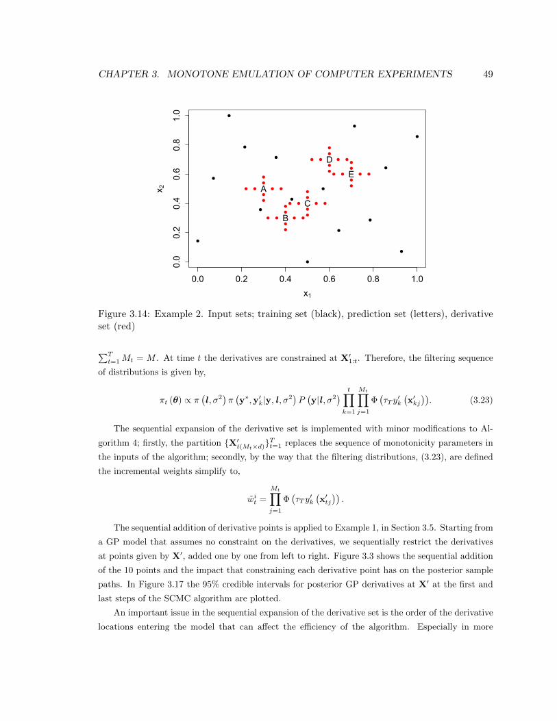
CHAPTER 3. MONOTONE EMULATION OF COMPUTER EXPERIMENTS 49
0.0 0.2 0.4 0.6 0.8 1.0
0.0
0.2
0.4
0.6
0.8
1.0
x1
x 2 A
B
C
D
E
Figure 3.14: Example 2. Input sets; training set (black), prediction set (letters), derivativeset (red)
∑Tt=1Mt = M . At time t the derivatives are constrained at X′1:t. Therefore, the filtering sequence
of distributions is given by,
πt (θ) ∝ π(l , σ2
)π(y∗,y′k|y, l , σ2
)P(y|l , σ2
) t∏k=1
Mt∏j=1
Φ(τT y′k
(x′kj)). (3.23)
The sequential expansion of the derivative set is implemented with minor modifications to Al-
gorithm 4; firstly, the partition {X′t(Mt×d)}Tt=1 replaces the sequence of monotonicity parameters in
the inputs of the algorithm; secondly, by the way that the filtering distributions, (3.23), are defined
the incremental weights simplify to,
wit =
Mt∏j=1
Φ(τT y′k
(x′tj)).
The sequential addition of derivative points is applied to Example 1, in Section 3.5. Starting from
a GP model that assumes no constraint on the derivatives, we sequentially restrict the derivatives
at points given by X′, added one by one from left to right. Figure 3.3 shows the sequential addition
of the 10 points and the impact that constraining each derivative point has on the posterior sample
paths. In Figure 3.17 the 95% credible intervals for posterior GP derivatives at X′ at the first and
last steps of the SCMC algorithm are plotted.
An important issue in the sequential expansion of the derivative set is the order of the derivative
locations entering the model that can affect the efficiency of the algorithm. Especially in more
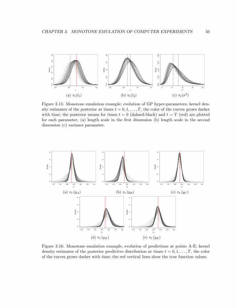
CHAPTER 3. MONOTONE EMULATION OF COMPUTER EXPERIMENTS 50
0.0 0.5 1.0 1.5
0.0
0.5
1.0
1.5
2.0
2.5
l1
Density
(a) πt(l1)
0.0 0.5 1.0 1.5
0.0
0.5
1.0
1.5
2.0
l2
Density
(b) πt(l2)
0 5 10 15 20
0.00
0.05
0.10
0.15
0.20
s2
Density
(c) πt(σ2)
Figure 3.15: Monotone emulation example; evolution of GP hyper-parameters; kernel den-sity estimates of the posterior at times t = 0, 1, . . . , T , the color of the curves grows darkerwith time; the posterior means for times t = 0 (dahsed-black) and t = T (red) are plottedfor each parameter; (a) length scale in the first dimension (b) length scale in the seconddimension (c) variance parameter.
-1.2 -1.0 -0.8 -0.6 -0.4 -0.2 0.0
02
46
8
yA
Density
(a) πt (yA)
-1.2 -1.0 -0.8 -0.6 -0.4 -0.2 0.0
02
46
8
yB
Density
(b) πt (yB)
-1.2 -1.0 -0.8 -0.6 -0.4 -0.2 0.0
02
46
8
yC
Density
(c) πt (yC)
-1.2 -1.0 -0.8 -0.6 -0.4 -0.2 0.0
02
46
8
yD
Density
(d) πt (yD)
-1.2 -1.0 -0.8 -0.6 -0.4 -0.2 0.0
02
46
8
yE
Density
(e) πt (yE)
Figure 3.16: Monotone emulation example; evolution of predictions at points A-E; kerneldensity estimates of the posterior predictive distribution at times t = 0, 1, . . . , T , the colorof the curves grows darker with time; the red vertical lines show the true function values.
CHAPTER 3. MONOTONE EMULATION OF COMPUTER EXPERIMENTS 51
0.5 0.6 0.7 0.8
-4-2
02
46
x'
y'(x)
(a) t = 0
0.5 0.6 0.7 0.8
-4-2
02
46
x'
y'(x)
(b) t = 10
Figure 3.17: The effect of sequential expansion of the derivative set on 95% credible intervals;the posterior mean (dashed lines) and credible bands obtained by (a) unconstrained GPmodel and (b) constrained model, together with the true function (red lines)
than one dimension it is not trivial how to progress through X′ to avoid particle degeneracy. The
problem arises from the fact that constraining the derivatives starting from a specific region of the
input space can encourage parameter values that make it impossible for the next derivative points
entering the model to be positive. A possible solution may be to define subsequent steps based on
the monotonicity parameter, τ , when the ESS is below a certain threshold. Possible directions for
addressing this issue are under investigation.
3.9 Discussion and future work
In this chapter we have developed a methodology for the incorporation of monotonicity information
into the GP emulation of a deterministic computer model. Through the mechanism of a link function,
monotonicity information is encoded via virtual derivatives (binary indicators of derivative sign) at
locations determined by a derivative input set. Some guidelines for construction of the derivative
input set are proposed while an online specification of the derivative design that can be assembled
into the sampling algorithm requires further investigation. Full inference for unsampled values of the
function and its derivatives are available via the proposed SCMC algorithm in Section 3.8 that uses
the parametrization of the constraints to sample from the posterior efficiently. Notably, by sampling
GP parameters l and σ, a more realistic representation of uncertainty is provided than would be
obtained from plug-in estimates of l and σ. Through examples, a simulation study, and a queueing
application, we demonstrate improvement in prediction uncertainty while respecting monotonicity
information.
The proposed methodology will be most effective in situations where monotonicity of the function

CHAPTER 3. MONOTONE EMULATION OF COMPUTER EXPERIMENTS 52
is not clear from the data. As Example 1 indicates, when the training set has gaps or holes, the lack
of nearby data points may lead conventional GP models to estimate a non-monotone relationship.
As the queueing application suggests, another challenging situation arises when the true function is
monotone but nearly constant. In both these situations, incorporating the monotonicity information
into the model is helpful, since the conventional GP model may infer a non-monotone relationship.
As input dimension increases, efficient computation becomes more of a consideration. If deriva-
tives are constrained in dm input dimensions, then monotonicity information is required in each of
these inputs. Increasing dm has the effect of increasing the size of the covariance matrix in (3.19)
that has to be inverted with each evaluation of the likelihood. This can slow down the computation
considerably. However, the SCMC algorithm (Chapter 2) used to sample from the posterior has the
advantage of being easily parallelizable and is shown to be stable as the dimensionality increases,
thereby, being able to handle fairly high-dimensional scenarios.
In applying the SCMC algorithm to monotone emulation of computer experiments, we have
proposed two methods for sequentially imposing the monotonicity constraint: increasing the mono-
tonicity parameter or increasing the size of the derivative set. While the performance of the first
method is demonstrated by our examples and simulation study, there are open questions to be
addressed about the second method that are under investigation.
Densely designed derivative sets are ideal choices that prevent the emulator from violating mono-
tonicity, at the cost of adding to the computation complexity. An alternative solution is to prevent
violations of the constraint by defining informative priors over the length scale parameters, thereby,
encouraging smooth response surfaces. Prior knowledge regarding the smoothness of the underlying
function, elicited from the monotonicity information, can be formulated in form of a (soft) lower
bound on the length scale parameter. This lower bound can then be translated into a maximum
level of sparsity in the derivative design. Elicitation of informative priors that permit smaller and
more sparse derivative sets and therefore more efficient computation, define subsequent steps of this
project.
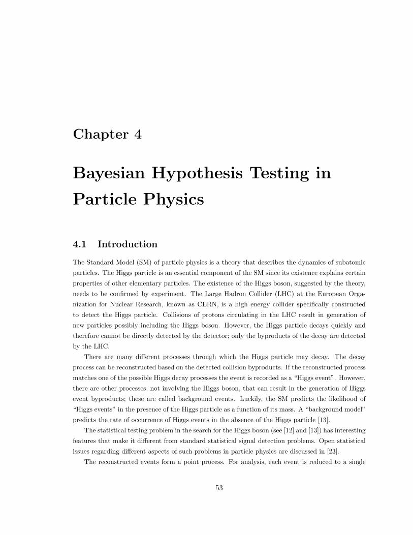
Chapter 4
Bayesian Hypothesis Testing in
Particle Physics
4.1 Introduction
The Standard Model (SM) of particle physics is a theory that describes the dynamics of subatomic
particles. The Higgs particle is an essential component of the SM since its existence explains certain
properties of other elementary particles. The existence of the Higgs boson, suggested by the theory,
needs to be confirmed by experiment. The Large Hadron Collider (LHC) at the European Orga-
nization for Nuclear Research, known as CERN, is a high energy collider specifically constructed
to detect the Higgs particle. Collisions of protons circulating in the LHC result in generation of
new particles possibly including the Higgs boson. However, the Higgs particle decays quickly and
therefore cannot be directly detected by the detector; only the byproducts of the decay are detected
by the LHC.
There are many different processes through which the Higgs particle may decay. The decay
process can be reconstructed based on the detected collision byproducts. If the reconstructed process
matches one of the possible Higgs decay processes the event is recorded as a “Higgs event”. However,
there are other processes, not involving the Higgs boson, that can result in the generation of Higgs
event byproducts; these are called background events. Luckily, the SM predicts the likelihood of
“Higgs events” in the presence of the Higgs particle as a function of its mass. A “background model”
predicts the rate of occurrence of Higgs events in the absence of the Higgs particle [13].
The statistical testing problem in the search for the Higgs boson (see [12] and [13]) has interesting
features that make it different from standard statistical signal detection problems. Open statistical
issues regarding different aspects of such problems in particle physics are discussed in [23].
The reconstructed events form a point process. For analysis, each event is reduced to a single
53
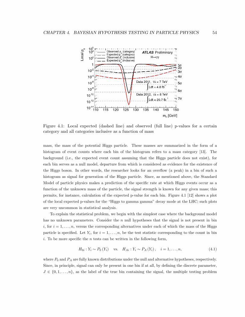
CHAPTER 4. BAYESIAN HYPOTHESIS TESTING IN PARTICLE PHYSICS 54
Figure 4.1: Local expected (dashed line) and observed (full line) p-values for a certaincategory and all categories inclusive as a function of mass
mass, the mass of the potential Higgs particle. These masses are summarized in the form of a
histogram of event counts where each bin of the histogram refers to a mass category [13]. The
background (i.e., the expected event count assuming that the Higgs particle does not exist), for
each bin serves as a null model, departure from which is considered as evidence for the existence of
the Higgs boson. In other words, the researcher looks for an overflow (a peak) in a bin of such a
histogram as signal for generation of the Higgs particle. Since, as mentioned above, the Standard
Model of particle physics makes a prediction of the specific rate at which Higgs events occur as a
function of the unknown mass of the particle, the signal strength is known for any given mass; this
permits, for instance, calculation of the expected p-value for each bin. Figure 4.1 [12] shows a plot
of the local expected p-values for the “Higgs to gamma gamma” decay mode at the LHC; such plots
are very uncommon in statistical analysis.
To explain the statistical problem, we begin with the simplest case where the background model
has no unknown parameters. Consider the n null hypotheses that the signal is not present in bin
i, for i = 1, . . . , n, versus the corresponding alternatives under each of which the mass of the Higgs
particle is specified. Let Yi, for i = 1, . . . , n, be the test statistic corresponding to the count in bin
i. To be more specific the n tests can be written in the following form,
H0i : Yi ∼ P0 (Yi) vs. HAi : Yi ∼ PA (Yi) , i = 1, . . . , n, (4.1)
where P0 and PA are fully known distributions under the null and alternative hypotheses, respectively.
Since, in principle, signal can only be present in one bin if at all, by defining the discrete parameter,
J ∈ {0, 1, . . . , n}, as the label of the true bin containing the signal, the multiple testing problem
CHAPTER 4. BAYESIAN HYPOTHESIS TESTING IN PARTICLE PHYSICS 55
reduces to a single test,
H0 : J = 0 vs. HA : J > 0, (4.2)
where J = 0 refers to the case that the particle does not exist.
The current procedure consists of two stages: detection and exclusion. In the detection stage, a
likelihood ratio test (LRT) is performed to test (4.2). False discovery is penalized heavily in particle
physics. Therefore, in order to announce a discovery, strong enough evidence (a 5-σ effect, or a p-
value smaller than about 3× 10⁻⁷) must be observed. (In high energy physics p-values are generally
reported as a normal score; a kσ significance level corresponds to a p-value of p = 1−Φ(k) where Φ
is the standard normal cumulative distribution function.)
If such strong evidence is not observed in the detection stage, one proceeds to the exclusion stage
where the nulls and alternatives in (4.1) are switched. This can be useful since the distributions are
fully specified under the alternative hypotheses. The n LRTs are performed independently, at a
significance level of α = 0.05, to exclude some of the bins while retaining others as locations where
continuing search may be carried out.
The ad hoc structure of the procedure just described motivates the work in the present chap-
ter. We develop a Bayesian alternative to the existing method that is statistically justifiable while
addressing the issues that physicists are concerned about, such as controlling false discovery rate.
We take a decision theoretic approach and define a linear loss function that captures the features
of the problem such as the known signal strength. The Bayes rule obtained for this loss function is
in the form of a threshold on the posterior odds for the parameter J and results in a set of possible
values for J referred to as the decision set. Our approach is similar to that in [15] but tailored to suit
the specific features of our application. Another interesting related work is that of [17] in which the
Higgs problem is visited; they simplify the model and ignore the known signal strength assumption
to facilitate analysis.
Our proposed Bayesian procedure does not depend on the model; it can be carried out regardless
of the choice of model as long as one can derive or estimate the posterior distribution of the parameter
of interest given the data with all the nuisance parameters integrated out. We use normal models
in the first part of this chapter. These models serve as toy problems: simplifications of the Higgs
search designed to help understand and evaluate the existing procedure and compare it to the Bayes
procedure.
Although the Bayes procedure is model-independent in terms of structure, its performance de-
pends on the adequacy of the model as for any other statistical procedure. Therefore, after intro-
ducing our Bayesian testing method and comparing it with the existing procedure for a simplified
model, we focus on a more realistic model that takes important aspects of the problem into account,
particularly uncertainty in the background model.
Current methods fit different parametric models, such as fourth-order polynomials and expo-
nential functions, to the background function (intensity function of the point process in the absence
CHAPTER 4. BAYESIAN HYPOTHESIS TESTING IN PARTICLE PHYSICS 56
of the Higgs particle) in different channels (a channel is one of the various possible decay processes
mentioned above); see [12], Section 5.5. Taking a nonparametric approach, we assume a Gaussian
process prior over the background intensity function and instead of using point estimates for the
background means, integrate them over their prior.
Unfortunately, privacy policies in the area of particle physics do not allow access to the real data
for non-members of the search group. Therefore, we apply the model to data simulated to imitate
the plots in [12] for a specific search channel for the Higgs problem. Recently, we received Monte
Carlo data that are generated by computer code that simulates the behavior of the LHC; analysis
of these simulated data and adapting our models to suit the additional layers of information defines
our next steps for this project.
4.2 The Existing Approach
In this section we give a simplified explanation of the existing procedure. We use a normal model
with no nuisance parameters. The same model is used to make comparisons between the current
and proposed procedures in Section 4.4.1.
Consider a normal approximation for the n statistics, Yi, i.e., let Yi, i = 1, . . . , n, be independent
normal random variables scaled to have unit variance. The mean of Yi is zero if signal is not present
in bin i and is the known quantity, si, if bin i is the true location of the signal. Therefore, the
problem can be formulated as testing the null hypothesis, H0, that the Higgs particle does not exist,
so that all the Yi’s are standard normal variables, versus the alternative hypothesis that the Higgs
boson exists with a certain mass determined by the known signal size, sj , i.e., there exists Yj whose
mean is sj and all the other Yi, i 6= j are standard normal.
The only unknown parameter under the above model is the location of the signal, the discrete
parameter, J . The parameter space is J = {0, 1, . . . , n}, where J = 0 represents the case that none
of the bins contains signal.
The currently used testing procedure comprises two stages: detection, where the researcher looks
for strong enough evidence to report a bin as the location of the signal; and exclusion, which follows
if the researcher fails to find such a strong evidence, i.e., fails to detect, and proceeds to further
investigation in order to exclude some of the bins as possible locations of the signal and narrow the
search to fewer number of locations.
When the two stages are complete a subset, S, of J will have been selected. In the following we
describe these two stages and the resulting set S in detail.
4.2.1 Detection
The hypothesis,
H0 : Yiiid∼ N (0, 1) , for i = 1, . . . , n, i.e., J = 0,
CHAPTER 4. BAYESIAN HYPOTHESIS TESTING IN PARTICLE PHYSICS 57
is tested against the alternative hypothesis,
HA : ∃j such that Yjiid∼ N (sj , 1) , i.e., J > 0,
where the vector of signal sizes, s = (s1, . . . , sn), is known. Let Y = (Y1, . . . , Yn) be the random
vector of the n statistics and y = (yi, . . . , yn) be the observed value of this random vector. The
likelihood function, L (J) = P (Y = y|J), under H0 and HA is given by the following expressions
respectively,
L (0) =
n∏i=1
φ (yi) ,
L (j) = {n∏i=1
φ(yi)} exp
(yjsj −
s2j2
), j = 1, . . . , n.
where φ(.) is the standard normal density function. Therefore, the likelihood ratio test statistic is of
the form,
Λ0 = −2 logL (0)
supk∈{1,...,n} L (k)= 2yJsJ − s
2J, (4.3)
where
J = argmaxi∈{1,...,n}(2yisi − s2i
). (4.4)
Surprisingly, the current detection procedures used in particle physics ignore the known signal sizes.
Instead, the current practice, interpreted in our toy problem, replaces Λ0 by
Λ∗0 = −2 logL(0)
supk∈{1,...,n} supsk>0 L(k)= yJ (4.5)
where
J = argmaxi∈{1,...,n}yi.
In Section 4.4.1 we consider the case where s1 = . . . = sn. In this case, J = J (see Appendix B for
proof) and the two likelihood functions are equivalent for testing purposes. In Section 4.4.2, however,
we compare current procedures, which are based on analogues of Λ∗0 to our Bayes procedure, and
not the formal LRT, in the known signal strength model. In Appendix C we investigate the impact
of ignoring the signal sizes, i.e., the use of (4.5) instead of (4.3), on the power of the test through a
simulation study.
In physics “discovery” traditionally requires a 5-σ effect which corresponds to a p-value below
3 × 10⁻⁷. So the type I error rate, i.e., probability of “false discovery” is chosen to be very small.
The critical value, c0, for the rejection region, R0 = {Λ0 > c0}, is determined to match this type I
error rate (α1 = 3× 10⁻⁷), i.e., by solving
n∏i=1
Φ
(c0 + s2i
2si
)≥ 1− α1.
The result of this stage of the testing procedure is one of the following:

CHAPTER 4. BAYESIAN HYPOTHESIS TESTING IN PARTICLE PHYSICS 58
• Λ0 ∈ R0, therefore the null hypothesis is rejected; let S = {J}, where S is the final decision,
i.e., signal is detected in bin J .
• Λ0 /∈ R0; proceed to the next stage, exclusion.
4.2.2 Exclusion
When the data does not yield enough evidence to announce the existence of the particle in the first
stage of the procedure, physicists are unwilling to stop the investigation and wish to extract more
information from the data. This further investigation is as follows.
Define the n null hypotheses,
H0i : Yi ∼ N (si, 1) , for i = 1, . . . , n,
versus the corresponding alternative hypotheses,
HAi : Yi ∼ N (0, 1) , for i = 1, . . . , n,
that are tested individually for each bin. This amounts to excluding as many bins as possible, as
likely locations of the signal. The likelihood ratio test statistics are given by,
Λi = −2 logL (i)
L (0)= s2i − 2yisi, i = 1, . . . , n.
The rejection regions, Ri = {Λi > ci}, are obtained with respect to the type I error rate, α2 (typically
physicists take α2 = 0.05),
ci = −s2i − 2siΦ−1 (α2) .
Note that, one does not need to correct for multiple comparisons in the exclusion stage since no more
than one of the null hypotheses can be true and therefore the family-wise type I error rate is in fact
α2.
The final decision set is S = {0} ∪ {i : Λi < ci, i = 1, . . . n}. Note that under the current
procedure, if 0 is not included in S, the cardinality of S cannot be greater than one. This happens
in the case that the researcher is convinced that the signal exists and makes a decision about the
location of it. When 0 ∈ S, the decision set, S, can contain more than one element in addition to
0, leading to the possibilities that either the signal does not exist or if it does, some likely locations
are provided while others are ruled out.
4.3 A Bayesian Testing Procedure
In this section we consider the problem from a decision theoretic point of view. We define a linear
loss function and derive the Bayes rule that can be used as an alternative to the current method for
reporting one or more possible locations for the signal. The Bayes procedure that can be calibrated
to match specified frequency theory error rates, is described in the following.
CHAPTER 4. BAYESIAN HYPOTHESIS TESTING IN PARTICLE PHYSICS 59
4.3.1 Structure
The required ingredients of a decision theory problem are a model with corresponding parameter
space, a decision space, i.e., a set of possible actions, and a loss function [3].
We consider a number of models with different levels of complexity through this chapter. How-
ever, the procedure is introduced regardless of the specific choice of the model. We define the decision
space as the set of all possible subsets, S ⊂ J . The loss function is defined in the following form,
L (J, S) =
CJ +∑j∈S
lj
1Sc (J) +
∑j∈S−{J}
lj
1S (J) , (4.6)
where CJ refers to the loss when the true value of the parameter is excluded, lj is the loss when j
is incorrectly included in S while J 6= j, for j = 0, 1, . . . , n, 1A (.) is the indicator function of set A,
and Sc is the complement of S.
As an intuitive interpretation of (4.6), suppose that J is the true value of the parameter, i.e.,
the location of the signal. The first expression on the right hand side of (4.6) is the loss that one is
penalized with for excluding J from the decision set that includes the loss of excluding the true value
of the parameter in addition to the loss of including any other value in S. The second term on the
right hand side of (4.6) refers to the case that J ∈ S. For such a decision set there is no exclusion
penalty and one is only charged with the loss of including any other possible values in S in addition
to J .
Consider the posterior probability mass function (pmf) of J given the observed data, y,
π (j | y) =π(j)P (y | J = j)∑nk=0 π(k)P (y | J = k)
, j = 0, 1, . . . , n, (4.7)
where π(j) = P (J = j), j = 0, 1, . . . , n, is the prior pmf on J . By averaging the loss function (4.6)
with respect to the posterior (4.7) the posterior expected loss or the posterior Bayes risk is obtained
as follows.
rπ(J|y) (S) = Eπ(J|y) (L (J, S))
= Eπ(J|y)
∑j∈S−{J}
lj
1S (J) +
CJ +∑j∈S
lj
1Sc (J)
=∑i∈S
∑j∈S−{i}
lj
π (i | y) +∑i∈Sc
Ci +∑j∈S
lj
π (i | y)
The Bayes rule is obtained by minimizing the posterior Bayes risk with respect to S;
Theorem 1. The Bayes rule, i.e., the decision rule that minimizes rπ(J|y)(S), is given by,
S = {j; j = 0, 1, . . . , n :π (j|y)
π (Θ− {j}|y)>
ljCj}.
CHAPTER 4. BAYESIAN HYPOTHESIS TESTING IN PARTICLE PHYSICS 60
Proof. Let S1 be a decision set where k ∈ S1. The posterior Bayes risk for S1 is of the following
form,
rπ(J|y) (S1) =∑
j∈S1−{k}
ljπ (k | y) +∑
i∈S1−{k}
lk +∑
j∈S1−{i,k}
lj
π (i | y)
+∑j∈Sc
1
Ci +
lk +∑
j∈S1−{k}
lj
π (i | y) .
Let S2 = S1 − {k}. The Bayes risk for this decision set is,
rπ(J|y) (S2) =∑i∈S2
∑j∈S2−{i}
lj
π (i | y) +
Ck +∑j∈S2
lj
π (k | y)
+∑
i∈Sc2−{k}
Ci +∑j∈S2
lj
π (i | y)
=∑
i∈S1−{k}
∑j∈S1−{i,k}
lj
π (i | y) +
Ck +∑
j∈S1−{k}
lj
π (k | y)
+∑i∈Sc
1
Ci +∑
j∈S1−{k}
lj
π (i | y) .
The decision set will contain k if,
rπ(J|y) (S1)− rπ(J|y) (S2) = lk
∑i∈S1−{k}
π (i | y) +∑i∈Sc
1
π (i | y)
− Ckπ (k | y)
= lkπ (Θ− {k} | y)− Ckπ (k | y) < 0.
Therefore, k ∈ S if,π (k | y)
π (Θ− {k} | y)>
lkCk
.
4.3.2 Calibration
As mentioned, the proposed procedure can be calibrated to satisfy frequency theory properties such
as the type I error rates. The loss ratios, lj/Cj , are considered as free parameters that can be
adjusted to match the type I error rates required in particle physics, i.e.,
P (0 /∈ SB | J = 0) = P
(π (0|y)
π (Θ− {0}|y)<
l0C0
)≤ 1− (1− α1)n,
CHAPTER 4. BAYESIAN HYPOTHESIS TESTING IN PARTICLE PHYSICS 61
P (j /∈ SB | J = j) = P
(π (j|y)
π (Θ− {j}|y)<
ljCj
)≤ α2,
where SB is the decision set obtained by the Bayes procedure. Solving the above equations for the
loss ratios, l0/C0 and lj/Cj , requires obtaining the 1− (1− α1)n100% and α2100% quantiles of the
null distributions of the posterior odds, π(0|y)/π(Θ− {0}|y) and π(j|y)/π(Θ− {j}|y).
Note that tuning the loss ratios to match the type I error rates is equivalent to tuning the prior
distribution, π(J). For example, consider the event, 0 ∈ S, which is decided by the following rule,
0 ∈ S ⇔ π (0 | |y)
π ({0}c | y)>
l0C0,
⇔ π (y | 0)
π (y | {0}c)π(0)
1− π(0)>
l0C0,
⇔ π (y | 0)
π (y | {0}c)>
l0C0
1− π(0)
π(0).
Thus, adjusting the ratio, l0/C0, is equivalent to adjusting (1−π(0))/π(0). Intuitively, when assuming
larger prior mass on H0 (large π(0)) one can compensate for it by penalizing a large loss value when
0 is included in S incorrectly (a larger l0). And similarly, if the prior assigns a larger weight to the
alternative, by increasing the loss when 0 is excluded incorrectly (C0), the decision rule remains the
same. Here, we keep the prior fixed and adjust the loss ratios.
Unfortunately, under most of the realistic models, even including most simplified models for the
Higgs problem considered in this paper, the distribution of the posterior odds cannot be obtained
in closed form. Recently, [17] developed the uniformly most powerful Bayesian test (UMPBT) for
one-parameter exponential family based on the same idea, i.e., maximizing the probability that the
Bayes factor is smaller than a certain threshold under the null model. The Higgs problem is visited
briefly in [17] and the size of a Bayes factor equivalent to the significance level of α1 = 3 × 10⁻⁷ is
obtained. However, to obtain the UMPBT, a normal model is assumed in [17] and the known signal
assumption which is the main characteristic of the Higgs application, is ignored.
Since we are anxious to investigate the impact of the known signal assumption, we need to
estimate percentiles of the distribution of the posterior odds using Monte Carlo. Algorithm 5 is the
Monte Carlo algorithm used for calibration.
Of course, simple Monte Carlo estimates for quantiles far in the tail of a distribution, for example
the one corresponding to the small detection significance level, are not accurate. Developing more
advanced Monte Carlo using sequential Monte Carlo techniques or/and using some approximate
method for faster calculation of the posterior odds that would allow for larger-scale Monte Carlo is
currently under investigation.
CHAPTER 4. BAYESIAN HYPOTHESIS TESTING IN PARTICLE PHYSICS 62
Algorithm 5 Monte Carlo algorithm to construct the Bayes procedure
Input: A specified model M(J,θ) where θ is the vector of nuisance parameters.1: for j := 0, 1, . . . , n do
Generate a sample of size N from the model; y1:N ∼M(J,θ).
Obtain rij = P (J=j|yi)P (J 6=j|yi)
, i = 1, . . . , N .
if j = 0 then l0C0← 100α1-th sample quantile of r1:N
0
elseljCj← 100α2-th sample quantile of r1:N
j
end if
2: end forReturn: Loss ratios
ljCj
, j = 0, 1, . . . , n.
4.4 Comparisons
In this section we make comparisons between the two procedures explained in the previous sections.
The statistical procedure currently in practice is known to a certain extent from the accessible
resources but the details, such as the exact models used for the background intensity function and
the known signal function parameters are not provided. Therefore, replicating the existing statistical
procedures for a real version of the problem is not possible. For this very reason, we are only able
to make the comparisons for simplified models that, while preserving the important features of the
problem such as known signal strength, permit implementation of the existing procedure.
However, we argue that the Bayesian testing procedure proposed can be implemented regardless
of the model. Therefore, the comparison results remain valid for more complex models as long as
the Bayes procedure can be calibrated to satisfy the frequentist type I error rates.
The two models considered in the following are the normal model introduced in Section 2 and
a model that indicates how the nuisance parameters and unequal signal sizes are dealt with in the
two procedures.
4.4.1 Model 1: Known Background Parameters, Equal Signal Sizes
In this section we describe a simulation study that compares the two procedures explained in the
previous sections in terms of a number of frequency theory criteria and the expected loss, for the
simplified model introduced in Section 4.2 with an additional level of hierarchy that defines a prior
distribution for the parameter of interest. More specifically, the data for the simulation study are
generated from the following model,
J ∼ π(j),
P (yi|J = j) = N (yi; 0, 1), for i 6= j
CHAPTER 4. BAYESIAN HYPOTHESIS TESTING IN PARTICLE PHYSICS 63
P (yj |J = j) = N (yj ; sj , 1),
where
π(j) =
{0.5 if j = 00.5n if j = 1, . . . , n,
(4.8)
and
sj = 3, j = 1, . . . , n.
To implement the existing procedure explained in Section 4.2, the rejection regions have to be
determined. At each stage, the critical values are obtained to satisfy a prespecified type I error rate.
To be more specific, the detection critical value, c0, is chosen such that,
P (∃j : 2yjsj − s2j > c0|J = 0) ≤ 1− (1− α1)n,
and the exclusion critical values are determined such that,
P (s2j − 2yjsj > cj |J = j) ≤ α2, j = 1, . . . , n.
Similarly, for the Bayes procedure the loss ratios need to be adjusted to obtain the desired type
I error rates. Algorithm 1 is used to determine the loss ratios. Note that for the simplified model
the exclusion and inclusion losses for j = 1, . . . , n are fixed, i.e., Cj = C and lj = l, since the signal
size, sj , is constant over the n bins.
As mentioned in Section 4.2, detection requires a 5-σ effect whose corresponding p-value is
3 × 10⁻⁷ but quantile estimates corresponding to such small tail probabilities using Monte Carlo
are inaccurate. Therefore, we use a larger type I error rate in the comparisons (α1 = 3 × 10⁻⁴) to
avoid large Monte Carlo errors in the calibration stage. A type I error rate of α2 = 0.05 is used for
exclusion.
When the critical values and the loss ratios are determined, the following performance measures
are estimated and compared for the both procedures through simulation;
β1 = P (0 ∈ S|J 6= 0),
β2 = P (j ∈ S|J 6= j, 0 ∈ S),
γ1 = P (j ∈ S|J = 0),
γ2 = P (j ∈ S|J 6= j),
RπB =
n∑j=0
∫L(j, S(y))π(j)p(y|j)dy,
where RπB is the Bayes risk. In general the error rates, β2, γ1 and γ2 depend on j, for j = 1, . . . , n.
However, in this example since sj are equal for all j, the error rates do not depend on j. Table 4.1
shows the estimates of the above criteria for the two procedures based on N = 1, 000, 000 simulations
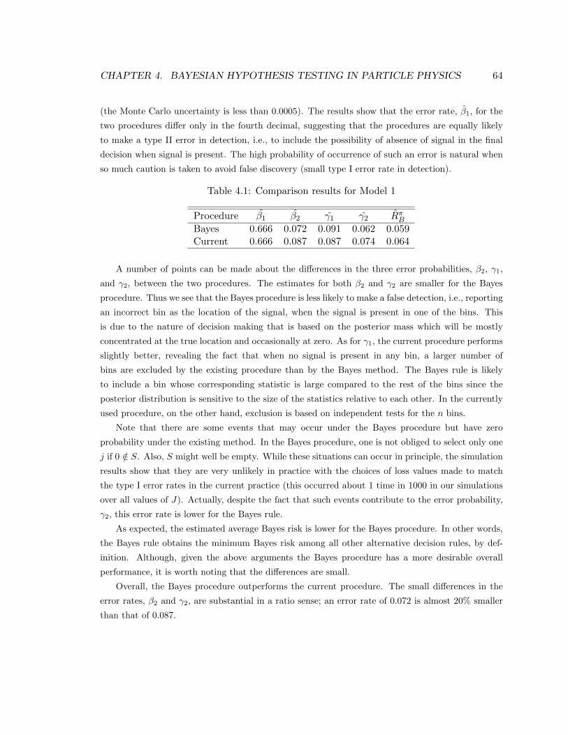
CHAPTER 4. BAYESIAN HYPOTHESIS TESTING IN PARTICLE PHYSICS 64
(the Monte Carlo uncertainty is less than 0.0005). The results show that the error rate, β1, for the
two procedures differ only in the fourth decimal, suggesting that the procedures are equally likely
to make a type II error in detection, i.e., to include the possibility of absence of signal in the final
decision when signal is present. The high probability of occurrence of such an error is natural when
so much caution is taken to avoid false discovery (small type I error rate in detection).
Table 4.1: Comparison results for Model 1
Procedure β1 β2 γ1 γ2 RπBBayes 0.666 0.072 0.091 0.062 0.059Current 0.666 0.087 0.087 0.074 0.064
A number of points can be made about the differences in the three error probabilities, β2, γ1,
and γ2, between the two procedures. The estimates for both β2 and γ2 are smaller for the Bayes
procedure. Thus we see that the Bayes procedure is less likely to make a false detection, i.e., reporting
an incorrect bin as the location of the signal, when the signal is present in one of the bins. This
is due to the nature of decision making that is based on the posterior mass which will be mostly
concentrated at the true location and occasionally at zero. As for γ1, the current procedure performs
slightly better, revealing the fact that when no signal is present in any bin, a larger number of
bins are excluded by the existing procedure than by the Bayes method. The Bayes rule is likely
to include a bin whose corresponding statistic is large compared to the rest of the bins since the
posterior distribution is sensitive to the size of the statistics relative to each other. In the currently
used procedure, on the other hand, exclusion is based on independent tests for the n bins.
Note that there are some events that may occur under the Bayes procedure but have zero
probability under the existing method. In the Bayes procedure, one is not obliged to select only one
j if 0 /∈ S. Also, S might well be empty. While these situations can occur in principle, the simulation
results show that they are very unlikely in practice with the choices of loss values made to match
the type I error rates in the current practice (this occurred about 1 time in 1000 in our simulations
over all values of J). Actually, despite the fact that such events contribute to the error probability,
γ2, this error rate is lower for the Bayes rule.
As expected, the estimated average Bayes risk is lower for the Bayes procedure. In other words,
the Bayes rule obtains the minimum Bayes risk among all other alternative decision rules, by def-
inition. Although, given the above arguments the Bayes procedure has a more desirable overall
performance, it is worth noting that the differences are small.
Overall, the Bayes procedure outperforms the current procedure. The small differences in the
error rates, β2 and γ2, are substantial in a ratio sense; an error rate of 0.072 is almost 20% smaller
than that of 0.087.
CHAPTER 4. BAYESIAN HYPOTHESIS TESTING IN PARTICLE PHYSICS 65
4.4.2 Model 2: Unknown Background, Unequal Signal Sizes
In this section, we introduce a nuisance parameter to the model; we consider the case where the
background means are unknown and have to be estimated. We continue working with the simplified
normal model where the n statistics are independent given the background means and signal location.
We assume that the unknown background mean is constant over the n bins; this is a very simple
model but one which serves as a useful illustration.
Signal size is an important factor in the sensitivity of the two procedures. Of course, a larger
signal size is easier to detect and the powers of the tests decrease as the signal sizes get smaller.
The plots of expected p-values given in [12] and [13] suggest that the known signal sizes are in
fact unequal. Therefore, an example that assumes variable signal sizes across the bins is worth
investigating to find out how the two procedures compare in this case. Again we explain the two
procedures and make comparisons in terms of frequentist error rates.
Let y = (y1, . . . , yn) be the vector of observed statistics, λ1 be the vector of unknown background
means and sj , for j = 0, 1, . . . , n, be a vector whose all elements are zero except for the jth element
which is equal to sj and, let s0 = (0, . . . , 0)T . The distribution of the “bin counts” given the model
parameters λ and sJ is given by a multivariate normal distribution,
P (y|λ, J) = N (y;λ1 + sJ , I),
where I is the identity matrix.
Despite the fact that the signal sizes, sj , are known the existing procedure takes the label of
the largest of yi as the estimated location of signal which is equivalent to replacing the signal sizes
by their maximum likelihood estimates (MLE) in a model where the sj are not known. To be more
specific, under the alternative hypothesis, J = j, the MLEs for the background nuisance parameter,
λ, and the signal sizes are respectively given by,
λj = y−j =1
n− 1
∑i6=j
yi,
and
sj =
{yj − y−j if yj − y−j > 0
0 if yj − y−j < 0.
By substituting these estimates into the likelihood the signal location, J , can be estimated by
J ′ = arg maxj
L(λj , sj)
= arg maxj,sj>0
{−∑i 6=j
(yi − y−j)2}
= arg maxj
yj .
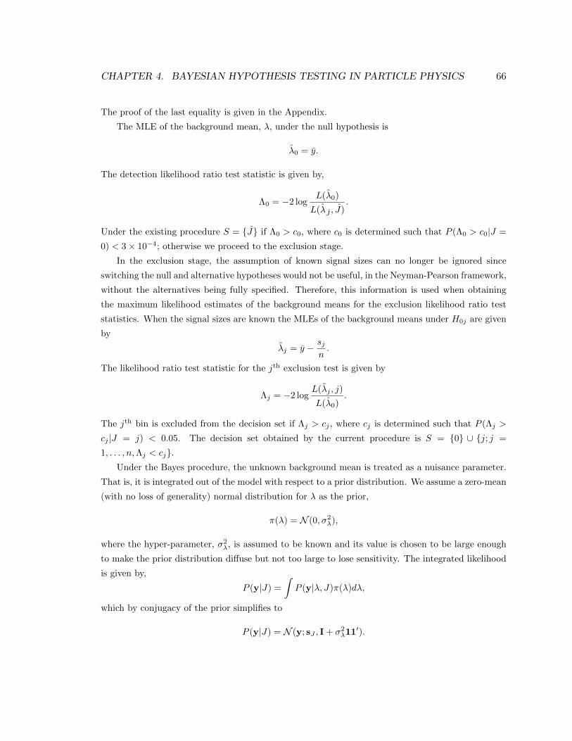
CHAPTER 4. BAYESIAN HYPOTHESIS TESTING IN PARTICLE PHYSICS 66
The proof of the last equality is given in the Appendix.
The MLE of the background mean, λ, under the null hypothesis is
λ0 = y.
The detection likelihood ratio test statistic is given by,
Λ0 = −2 logL(λ0)
L(λJ , J).
Under the existing procedure S = {J} if Λ0 > c0, where c0 is determined such that P (Λ0 > c0|J =
0) < 3× 10⁻⁴; otherwise we proceed to the exclusion stage.
In the exclusion stage, the assumption of known signal sizes can no longer be ignored since
switching the null and alternative hypotheses would not be useful, in the Neyman-Pearson framework,
without the alternatives being fully specified. Therefore, this information is used when obtaining
the maximum likelihood estimates of the background means for the exclusion likelihood ratio test
statistics. When the signal sizes are known the MLEs of the background means under H0j are given
by
λj = y − sjn.
The likelihood ratio test statistic for the jth exclusion test is given by
Λj = −2 logL(λj , j)
L(λ0).
The jth bin is excluded from the decision set if Λj > cj , where cj is determined such that P (Λj >
cj |J = j) < 0.05. The decision set obtained by the current procedure is S = {0} ∪ {j; j =
1, . . . , n,Λj < cj}.Under the Bayes procedure, the unknown background mean is treated as a nuisance parameter.
That is, it is integrated out of the model with respect to a prior distribution. We assume a zero-mean
(with no loss of generality) normal distribution for λ as the prior,
π(λ) = N (0, σ2λ),
where the hyper-parameter, σ2λ, is assumed to be known and its value is chosen to be large enough
to make the prior distribution diffuse but not too large to lose sensitivity. The integrated likelihood
is given by,
P (y|J) =
∫P (y|λ, J)π(λ)dλ,
which by conjugacy of the prior simplifies to
P (y|J) = N (y; sJ , I + σ2λ11
′).
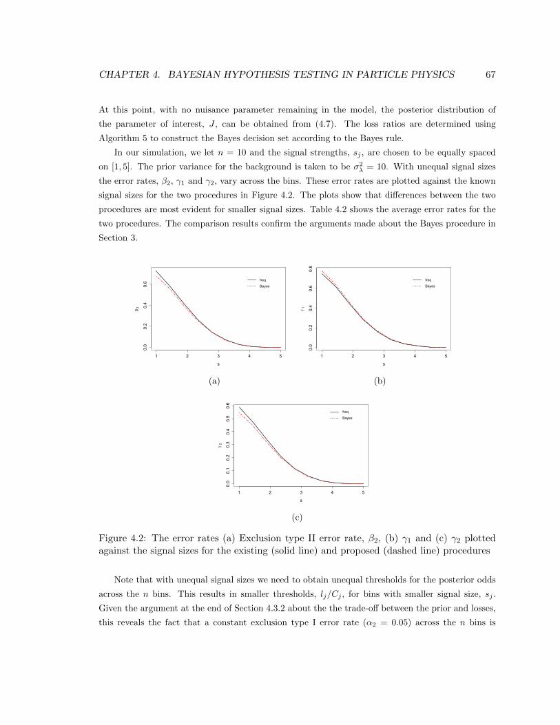
CHAPTER 4. BAYESIAN HYPOTHESIS TESTING IN PARTICLE PHYSICS 67
At this point, with no nuisance parameter remaining in the model, the posterior distribution of
the parameter of interest, J , can be obtained from (4.7). The loss ratios are determined using
Algorithm 5 to construct the Bayes decision set according to the Bayes rule.
In our simulation, we let n = 10 and the signal strengths, sj , are chosen to be equally spaced
on [1, 5]. The prior variance for the background is taken to be σ2λ = 10. With unequal signal sizes
the error rates, β2, γ1 and γ2, vary across the bins. These error rates are plotted against the known
signal sizes for the two procedures in Figure 4.2. The plots show that differences between the two
procedures are most evident for smaller signal sizes. Table 4.2 shows the average error rates for the
two procedures. The comparison results confirm the arguments made about the Bayes procedure in
Section 3.
1 2 3 4 5
0.0
0.2
0.4
0.6
s
b 2
freq
Bayes
(a)
1 2 3 4 5
0.0
0.2
0.4
0.6
0.8
s
g 1
freq
Bayes
(b)
1 2 3 4 5
0.0
0.1
0.2
0.3
0.4
0.5
0.6
s
g 2
freq
Bayes
(c)
Figure 4.2: The error rates (a) Exclusion type II error rate, β2, (b) γ1 and (c) γ2 plottedagainst the signal sizes for the existing (solid line) and proposed (dashed line) procedures
Note that with unequal signal sizes we need to obtain unequal thresholds for the posterior odds
across the n bins. This results in smaller thresholds, lj/Cj , for bins with smaller signal size, sj .
Given the argument at the end of Section 4.3.2 about the the trade-off between the prior and losses,
this reveals the fact that a constant exclusion type I error rate (α2 = 0.05) across the n bins is
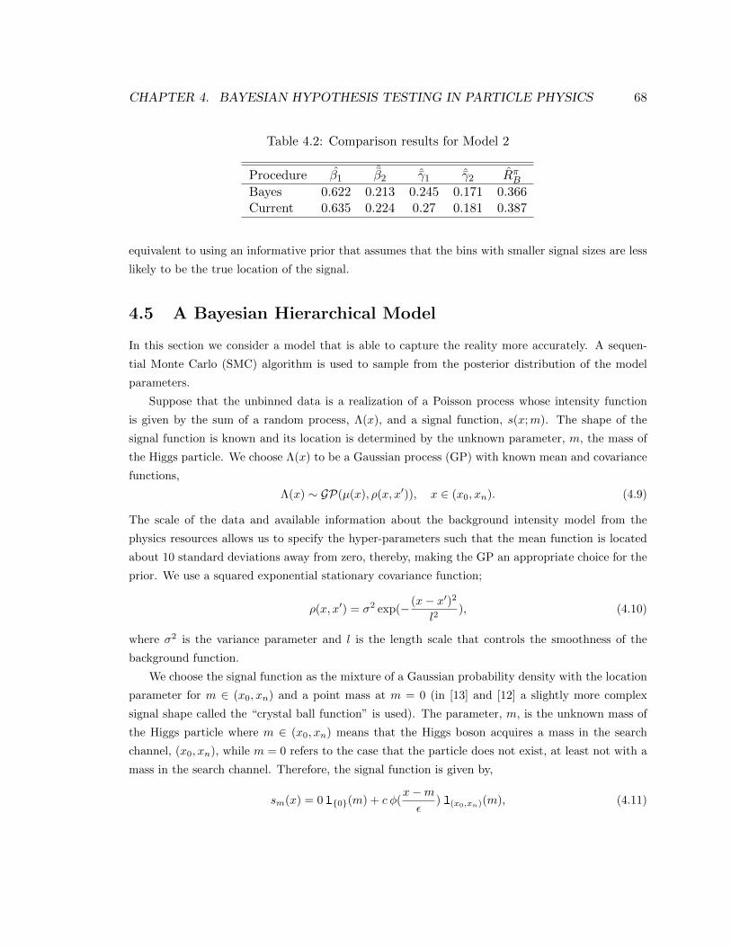
CHAPTER 4. BAYESIAN HYPOTHESIS TESTING IN PARTICLE PHYSICS 68
Table 4.2: Comparison results for Model 2
Procedure β1ˆβ2 ˆγ1 ˆγ2 RπB
Bayes 0.622 0.213 0.245 0.171 0.366Current 0.635 0.224 0.27 0.181 0.387
equivalent to using an informative prior that assumes that the bins with smaller signal sizes are less
likely to be the true location of the signal.
4.5 A Bayesian Hierarchical Model
In this section we consider a model that is able to capture the reality more accurately. A sequen-
tial Monte Carlo (SMC) algorithm is used to sample from the posterior distribution of the model
parameters.
Suppose that the unbinned data is a realization of a Poisson process whose intensity function
is given by the sum of a random process, Λ(x), and a signal function, s(x;m). The shape of the
signal function is known and its location is determined by the unknown parameter, m, the mass of
the Higgs particle. We choose Λ(x) to be a Gaussian process (GP) with known mean and covariance
functions,
Λ(x) ∼ GP(µ(x), ρ(x, x′)), x ∈ (x0, xn). (4.9)
The scale of the data and available information about the background intensity model from the
physics resources allows us to specify the hyper-parameters such that the mean function is located
about 10 standard deviations away from zero, thereby, making the GP an appropriate choice for the
prior. We use a squared exponential stationary covariance function;
ρ(x, x′) = σ2 exp(− (x− x′)2
l2), (4.10)
where σ2 is the variance parameter and l is the length scale that controls the smoothness of the
background function.
We choose the signal function as the mixture of a Gaussian probability density with the location
parameter for m ∈ (x0, xn) and a point mass at m = 0 (in [13] and [12] a slightly more complex
signal shape called the “crystal ball function” is used). The parameter, m, is the unknown mass of
the Higgs particle where m ∈ (x0, xn) means that the Higgs boson acquires a mass in the search
channel, (x0, xn), while m = 0 refers to the case that the particle does not exist, at least not with a
mass in the search channel. Therefore, the signal function is given by,
sm(x) = 0 1{0}(m) + c φ(x−mε
) 1(x0,xn)(m), (4.11)
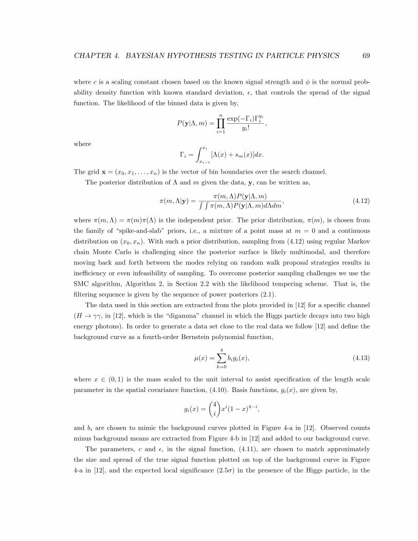
CHAPTER 4. BAYESIAN HYPOTHESIS TESTING IN PARTICLE PHYSICS 69
where c is a scaling constant chosen based on the known signal strength and φ is the normal prob-
ability density function with known standard deviation, ε, that controls the spread of the signal
function. The likelihood of the binned data is given by,
P (y|Λ,m) =
n∏i=1
exp(−Γi)Γyii
yi!,
where
Γi =
∫ xi
xi−1
[Λ(x) + sm(x)]dx.
The grid x = (x0, x1, . . . , xn) is the vector of bin boundaries over the search channel.
The posterior distribution of Λ and m given the data, y, can be written as,
π(m,Λ|y) =π(m,Λ)P (y|Λ,m)∫ ∫π(m,Λ)P (y|Λ,m)dΛdm
, (4.12)
where π(m,Λ) = π(m)π(Λ) is the independent prior. The prior distribution, π(m), is chosen from
the family of “spike-and-slab” priors, i.e., a mixture of a point mass at m = 0 and a continuous
distribution on (x0, xn). With such a prior distribution, sampling from (4.12) using regular Markov
chain Monte Carlo is challenging since the posterior surface is likely multimodal, and therefore
moving back and forth between the modes relying on random walk proposal strategies results in
inefficiency or even infeasibility of sampling. To overcome posterior sampling challenges we use the
SMC algorithm, Algorithm 2, in Section 2.2 with the likelihood tempering scheme. That is, the
filtering sequence is given by the sequence of power posteriors (2.1).
The data used in this section are extracted from the plots provided in [12] for a specific channel
(H → γγ, in [12], which is the “digamma” channel in which the Higgs particle decays into two high
energy photons). In order to generate a data set close to the real data we follow [12] and define the
background curve as a fourth-order Bernstein polynomial function,
µ(x) =
4∑k=0
bigi(x), (4.13)
where x ∈ (0, 1) is the mass scaled to the unit interval to assist specification of the length scale
parameter in the spatial covariance function, (4.10). Basis functions, gi(x), are given by,
gi(x) =
(4
i
)xi(1− x)4−i,
and bi are chosen to mimic the background curves plotted in Figure 4-a in [12]. Observed counts
minus background means are extracted from Figure 4-b in [12] and added to our background curve.
The parameters, c and ε, in the signal function, (4.11), are chosen to match approximately
the size and spread of the true signal function plotted on top of the background curve in Figure
4-a in [12], and the expected local significance (2.5σ) in the presence of the Higgs particle, in the
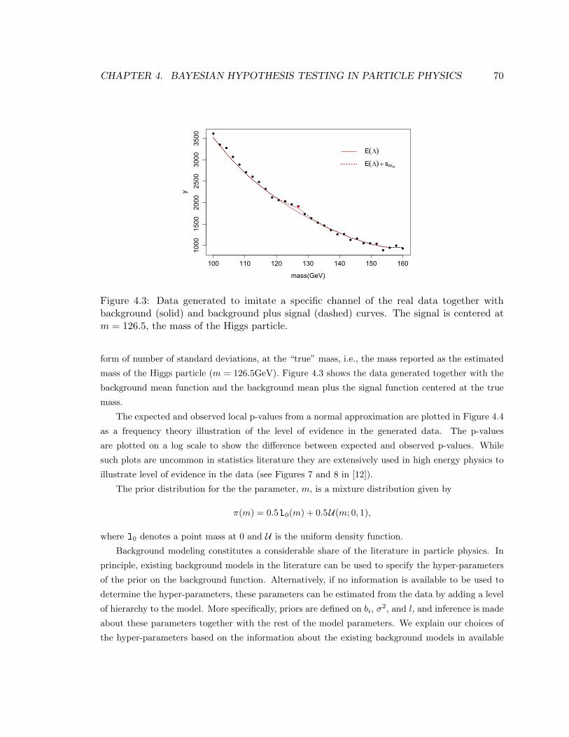
CHAPTER 4. BAYESIAN HYPOTHESIS TESTING IN PARTICLE PHYSICS 70
100 110 120 130 140 150 160
1000
1500
2000
2500
3000
3500
mass(GeV)
y
E(L)E(L) + smH
Figure 4.3: Data generated to imitate a specific channel of the real data together withbackground (solid) and background plus signal (dashed) curves. The signal is centered atm = 126.5, the mass of the Higgs particle.
form of number of standard deviations, at the “true” mass, i.e., the mass reported as the estimated
mass of the Higgs particle (m = 126.5GeV). Figure 4.3 shows the data generated together with the
background mean function and the background mean plus the signal function centered at the true
mass.
The expected and observed local p-values from a normal approximation are plotted in Figure 4.4
as a frequency theory illustration of the level of evidence in the generated data. The p-values
are plotted on a log scale to show the difference between expected and observed p-values. While
such plots are uncommon in statistics literature they are extensively used in high energy physics to
illustrate level of evidence in the data (see Figures 7 and 8 in [12]).
The prior distribution for the the parameter, m, is a mixture distribution given by
π(m) = 0.510(m) + 0.5U(m; 0, 1),
where 10 denotes a point mass at 0 and U is the uniform density function.
Background modeling constitutes a considerable share of the literature in particle physics. In
principle, existing background models in the literature can be used to specify the hyper-parameters
of the prior on the background function. Alternatively, if no information is available to be used to
determine the hyper-parameters, these parameters can be estimated from the data by adding a level
of hierarchy to the model. More specifically, priors are defined on bi, σ2, and l, and inference is made
about these parameters together with the rest of the model parameters. We explain our choices of
the hyper-parameters based on the information about the existing background models in available
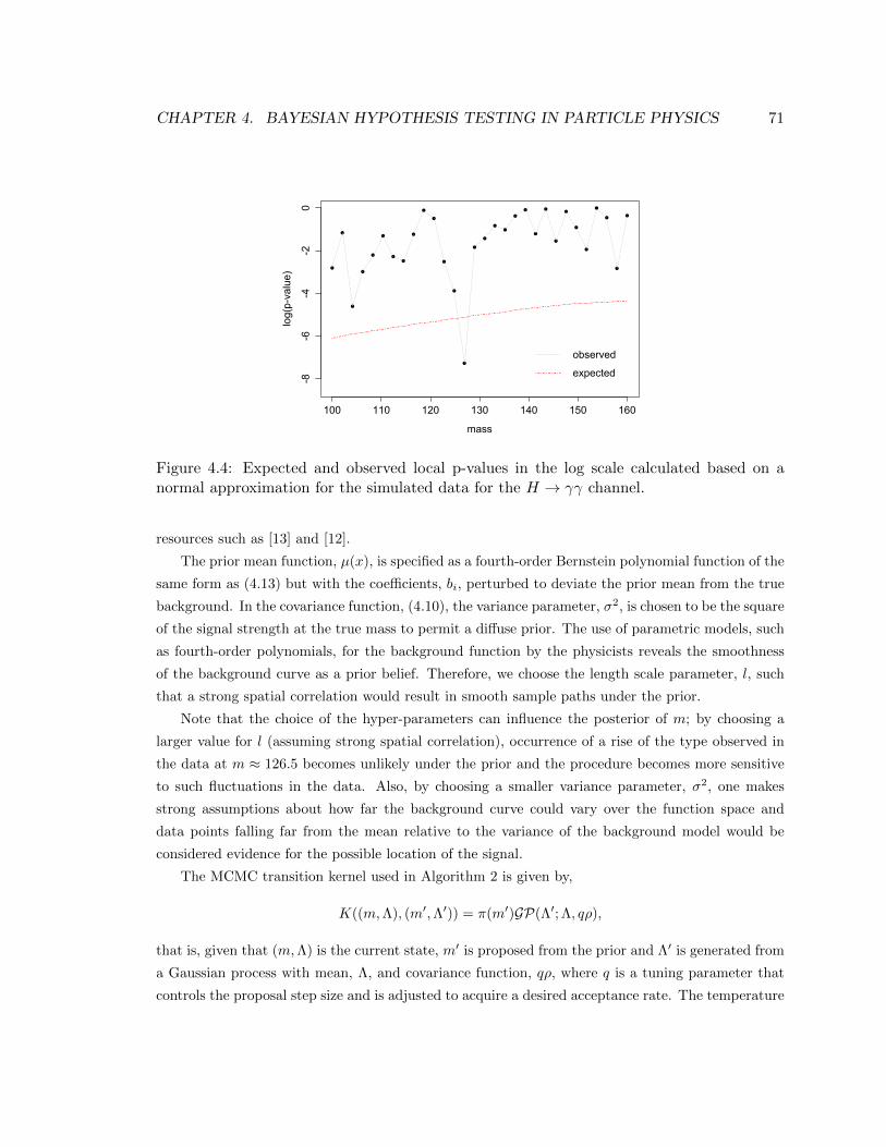
CHAPTER 4. BAYESIAN HYPOTHESIS TESTING IN PARTICLE PHYSICS 71
100 110 120 130 140 150 160
-8-6
-4-2
0
mass
log(p-value)
observed
expected
Figure 4.4: Expected and observed local p-values in the log scale calculated based on anormal approximation for the simulated data for the H → γγ channel.
resources such as [13] and [12].
The prior mean function, µ(x), is specified as a fourth-order Bernstein polynomial function of the
same form as (4.13) but with the coefficients, bi, perturbed to deviate the prior mean from the true
background. In the covariance function, (4.10), the variance parameter, σ2, is chosen to be the square
of the signal strength at the true mass to permit a diffuse prior. The use of parametric models, such
as fourth-order polynomials, for the background function by the physicists reveals the smoothness
of the background curve as a prior belief. Therefore, we choose the length scale parameter, l, such
that a strong spatial correlation would result in smooth sample paths under the prior.
Note that the choice of the hyper-parameters can influence the posterior of m; by choosing a
larger value for l (assuming strong spatial correlation), occurrence of a rise of the type observed in
the data at m ≈ 126.5 becomes unlikely under the prior and the procedure becomes more sensitive
to such fluctuations in the data. Also, by choosing a smaller variance parameter, σ2, one makes
strong assumptions about how far the background curve could vary over the function space and
data points falling far from the mean relative to the variance of the background model would be
considered evidence for the possible location of the signal.
The MCMC transition kernel used in Algorithm 2 is given by,
K((m,Λ), (m′,Λ′)) = π(m′)GP(Λ′; Λ, qρ),
that is, given that (m,Λ) is the current state, m′ is proposed from the prior and Λ′ is generated from
a Gaussian process with mean, Λ, and covariance function, qρ, where q is a tuning parameter that
controls the proposal step size and is adjusted to acquire a desired acceptance rate. The temperature
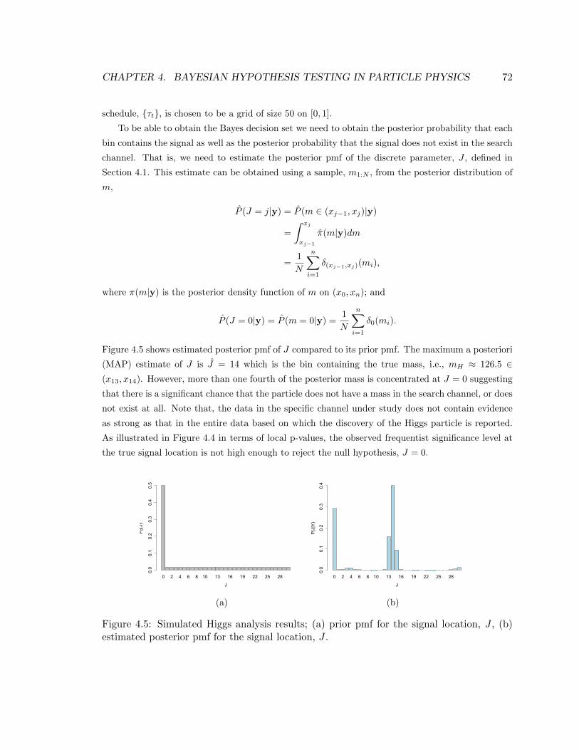
CHAPTER 4. BAYESIAN HYPOTHESIS TESTING IN PARTICLE PHYSICS 72
schedule, {τt}, is chosen to be a grid of size 50 on [0, 1].
To be able to obtain the Bayes decision set we need to obtain the posterior probability that each
bin contains the signal as well as the posterior probability that the signal does not exist in the search
channel. That is, we need to estimate the posterior pmf of the discrete parameter, J , defined in
Section 4.1. This estimate can be obtained using a sample, m1:N , from the posterior distribution of
m,
P (J = j|y) = P (m ∈ (xj−1, xj)|y)
=
∫ xj
xj−1
π(m|y)dm
=1
N
n∑i=1
δ(xj−1,xj)(mi),
where π(m|y) is the posterior density function of m on (x0, xn); and
P (J = 0|y) = P (m = 0|y) =1
N
n∑i=1
δ0(mi).
Figure 4.5 shows estimated posterior pmf of J compared to its prior pmf. The maximum a posteriori
(MAP) estimate of J is J = 14 which is the bin containing the true mass, i.e., mH ≈ 126.5 ∈(x13, x14). However, more than one fourth of the posterior mass is concentrated at J = 0 suggesting
that there is a significant chance that the particle does not have a mass in the search channel, or does
not exist at all. Note that, the data in the specific channel under study does not contain evidence
as strong as that in the entire data based on which the discovery of the Higgs particle is reported.
As illustrated in Figure 4.4 in terms of local p-values, the observed frequentist significance level at
the true signal location is not high enough to reject the null hypothesis, J = 0.
0 2 4 6 8 10 13 16 19 22 25 28
J
P0(J)
0.0
0.1
0.2
0.3
0.4
0.5
(a)
0 2 4 6 8 10 13 16 19 22 25 28
J
P(J|Y)
0.0
0.1
0.2
0.3
0.4
(b)
Figure 4.5: Simulated Higgs analysis results; (a) prior pmf for the signal location, J , (b)estimated posterior pmf for the signal location, J .
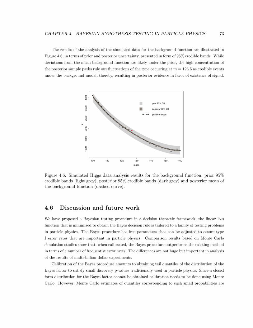
CHAPTER 4. BAYESIAN HYPOTHESIS TESTING IN PARTICLE PHYSICS 73
The results of the analysis of the simulated data for the background function are illustrated in
Figure 4.6, in terms of prior and posterior uncertainty, presented in form of 95% credible bands. While
deviations from the mean background function are likely under the prior, the high concentration of
the posterior sample paths rule out fluctuations of the type occurring at m = 126.5 as credible events
under the background model, thereby, resulting in posterior evidence in favor of existence of signal.
100 110 120 130 140 150 160
1000
1500
2000
2500
3000
3500
mass
y
prior 95% CB
posterior 95% CB
posterior mean
Figure 4.6: Simulated Higgs data analysis results for the background function; prior 95%credible bands (light grey), posterior 95% credible bands (dark grey) and posterior mean ofthe background function (dashed curve).
4.6 Discussion and future work
We have proposed a Bayesian testing procedure in a decision theoretic framework; the linear loss
function that is minimized to obtain the Bayes decision rule is tailored to a family of testing problems
in particle physics. The Bayes procedure has free parameters that can be adjusted to assure type
I error rates that are important in particle physics. Comparison results based on Monte Carlo
simulation studies show that, when calibrated, the Bayes procedure outperforms the existing method
in terms of a number of frequentist error rates. The differences are not huge but important in analysis
of the results of multi-billion dollar experiments.
Calibration of the Bayes procedure amounts to obtaining tail quantiles of the distribution of the
Bayes factor to satisfy small discovery p-values traditionally used in particle physics. Since a closed
form distribution for the Bayes factor cannot be obtained calibration needs to be done using Monte
Carlo. However, Monte Carlo estimates of quantiles corresponding to such small probabilities are

CHAPTER 4. BAYESIAN HYPOTHESIS TESTING IN PARTICLE PHYSICS 74
inaccurate. Possible solutions to address calibration issues are development of more advanced Monte
Carlo based on importance sampling or using extreme value theory to obtain approximate closed
form estimates.
A hierarchical Bayesian model is suggested to address Bayesian inference as well as decision
making in this application. The results of the fit of the model are illustrated as posterior distributions
of the model parameters and are in agreement with the results reported in the physics literature.
However, no formal comparison was made for the realistic version of the problem since the details of
the existing method and the real data has not been accessible.
We have recently been allowed access to Monte Carlo data that are generated by computer code
that simulates the detectors’ behavior and therefore can be used instead of the real data. This data
set that correspond to the H → γγ channel comprises a set of background events for nine “analysis
categories” and realizations of the signal function at a number of mass values. Our plan for analysis
of these data summarizes into the following; i) fitting a parametric model to the background data
that will later serve as the mean function for the Gaussian process prior over the background, ii)
interpolation (and extrapolation) of the signal function by fitting our Gaussian signal function to the
available realizations and estimating the variance and the signal strength, iii) constructing a signal
plus background data set by generating from the estimated signal function at the “true” mass and
adding these “signal events” to the background data, iv) analyze the constructed data set using the
model proposed in Section 4.5.
Chapter 5
Conclusion
In this thesis we have developed Bayesian procedures and computational methods for two indepen-
dent problems: constrained emulation of computer experiments and search for a new particle. The
computational tool required for sampling from the posterior distributions appearing throughout the
thesis were introduced in Chapter 2. The developed sampling algorithm is shown to be applicable
to a variety of problems in Bayesian inference where imposition of constraints creates difficulties in
posterior sampling.
Our proposed model for emulation of monotone computer experiments amounts to adding the
monotonicity information to the likelihood with a specific parametrization that assures local positiv-
ity constraints over the derivatives in the limit. While monotonicity of the predictions is not guaran-
teed by imposition of the constraint at a finite number of locations, when the sample paths are smooth
violation of monotonicity becomes unlikely in between these locations. This very parametrization
of the monotonicity constraint is used for efficient Monte Carlo sampling from the posterior that is
based on gradual imposition of the constraint in a sequential manner through importance sampling
and resampling steps. The performance of the proposed methodology is demonstrated by two exam-
ples, a simulation study and a real application. Comparisons between typical GP emulation and the
constrained model show an improvement in the quality of predictions in terms of the compatibility
with the monotonicity assumptions and uncertainty reduction.
We have also proposed a Bayesian procedure for a family of problems that arise in high energy
physics. The analysis of data collected from detectors that are used for discovery of a new particle is
considered. Our proposed procedure captures the current multi-stage detection/exclusion method in
a formal decision theoretic framework. The features of the problem are parametrized in a linear loss
function and the Bayes rule is obtained in the form of a threshold on the posterior odds of possible
mass values. The result of the analysis is a set of possible masses for the Higgs particle. If the data
provides evidence for discovery the resulting set does not include zero.
75
Bibliography
[1] N. Bambos and G. Michailidis. Queueing and scheduling in random environments.Advances in Applied Probability, 36:293–317, 2004. 42
[2] M. Beaumont, J. M. Cornuet, J. M. Marin, and C. Robert. Adaptive approximatebayesian computation. Biometrika, 96:983990, 2009. 16
[3] J. O. Berger. Statistical Decision Theory and Bayesian Analysis. Springer-Verlag NewYork Inc., 1980. 59
[4] J. O. Berger, V. De Oliveira, and B Sanso. Objective bayesian analysis of spatiallycorrelated data, journal of the amerian statistician association. Ann. Statist., 96:1361–1374, 2001. 47
[5] A. Beskos, D. Crisan, and A. Jasra. On the stability of sequential monte carlo methodsin high dimensions. arXiv:1103.3965v2, 2012. 34
[6] G. E. P. Box and G. C. Tiao. Bayesian Inference in Statistical Analysis. Wiley, 1973.10
[7] D. A. Campbell and S. Lele. An anova test for parameter estimability using datacloning with application to statistical inference for dynamic systems. ComputationalStatistics and Data Analysis, http://dx.doi.org/10.1016/j.csda.2013.09.013, 2013. 13
[8] David Campbell and Russell J. Steele. Smooth functional tempering for nonlineardifferential equation models. Statistics and Computing, 2011. 10
[9] A. C. Davison. Statistical Models. 94-160, 456-458, 605-619. Cambridge UniversityPress, 2003. 17
[10] H. Dette, Neumeyer. N., and K. F. Pilz. A simple nonparametric estimator of a strictlymonotone regression function. Bernoulli, 12:469–490, 2006. 22
[11] A. Doucet, N. De Freitas, and N.J. Gordon, editors. Sequential Monte Carlo Methodsin Practice. Springer-Verlag, 2001. 6
[12] G. Aad et al. [ATLAS Collaboration]. Observation of a new particle in the search forthe standard model higgs boson with the atlas detector at the lhc. Physics Letters B,716:1–29, 2012. 53, 54, 56, 65, 68, 69, 70, 71
76
BIBLIOGRAPHY 77
[13] S. Chatrchyan et al. [CMS Collaboration]. Observation of a new boson at a mass of125 gev with the cms experiment at the lhc. Physics Letters B, 716:30–61, 2012. 53,54, 65, 68, 71
[14] A. Gelman, F. Y. Bois, and J. Jiang. Physiological pharmacokinetic analysis usingpopulation modeling and informative prior distributions. Journal of the AmericanStatistical Association, 91(436):1400–1412, 1996. 10
[15] M. Guindani, P. Mller, and S. Zhang. A bayesian discovery procedure. J. R. Statist.Soc. B, 71:905–925, 2009. 55
[16] X. He and P. Shi. Monotone b-spline smoothing. Journal of the American StatisticalAssociation, 93:643–650, 1998. 22
[17] V. E. Johnson. Uniformly most powerful bayesian tests. The Annals of Statistics,41:1716–1741, 2013. 55, 61
[18] D. R. Jones, M. Schonlau, and W. J. Welch. Efficient global optimization of expensiveblack-box functions. Journal of Global Optimization, 13:455–492, 1998. 28
[19] P. Joyce and P. Marjoram. Approximately sufficient statistics and bayesian computa-tion. Statistical Applications in Genetics and Molecular Biology, 7, 2008. 16
[20] H. Kleijnin, J. P. C. and W. C. M. van Beers. Monotonicity-preserving bootstrappedkriging metamodels for expensive simulations. Journal of the Operational ResearchSociety, 64:708717, 2013. 23
[21] J. L. Leoppky, J. Sacks, and W. J. Welch. Choosing the sample size of a computerexperiment: A practical guide. Technometrics, 51:366–376, 2009. 30
[22] L. Lin and D. B. Dunson. Bayesian monotone regression using gaussian process pro-jection. 2013. 23, 80
[23] L. Lyons. Open statistical issues in particle physics. The Annals of Applied Statistics,2:887–915, 2008. 53
[24] J. M. Marin, P. Pudlo, C. P. Robert, and R. J. Ryder. Approximate bayesian compu-tational methods. Statistics and Computing, 22:1167–1180, 2012. 16
[25] E. Massad, F.A.B. Coutinho, M.N. Burattini, and L.F. Lopez. The eyam plague re-visited: did the village isolation change transmission from fleas to pulmonary? Med.Hypotheses, 63:911915, 2004. 13
[26] T. P. Minka. A Family of Algorithms for Approximate Bayesian Inference. PhD thesis,Massachusetts Institute of Technology, 2001. 23, 33
[27] P.D. Moral, A. Doucet, and A. Jasra. Sequential monte carlo samplers. J. R. Statist.Soc. B, 68:411436, 2006. 1, 4, 5, 6, 7
BIBLIOGRAPHY 78
[28] P.D. Moral, A. Doucet, and A. Jasra. An adaptive sequential monte carlo method forapproximate bayesian computation. Technical report, University of British Columbia,2009. 16
[29] M. D. Morris, T. J. Mitchell, and D. Ylvisker. Bayesian design and analysis of computerexperiments: use of derivatives in surface prediction. Technometrics, 35:243–255, 1993.22, 28
[30] N. J. R. Nelson J. R. Fagundes, N. Ray, M. Beaumont, S. Neuenschwander, F. M.M. Salzano, S. L. Bonatto, and L. Excofer. Statistical evaluation of alternative modelsof human evolution. Proc Natl Acad Sci USA, 104:17614–17619, 2007. 16
[31] E. Parzen. Stochastic Processes. San Francisco: Holden Day, 1962. 27
[32] J. O. Ramsay. Estimating smooth monotone functions. Journal of the Royal StatisticalSociety. Series B., 60:365–375, 1998. 22
[33] P. Ranjan, D. Bingham, and G. Michailidis. Sequential experiment design for contourestimation from complex computer codes. Technometrics, 50:527–541, 2008. 42
[34] Carl Edward Rasmussen and Christopher K. I. Williams. Gaussian Processes for Ma-chine Learning. MIT Press, Cambridge, Massachusetts, 2006. 24
[35] n O. Ratman, C. Andrieu, C. Wiuf, and S. Richardson. Model criticism based onlikelihood-free inference, with an application to protein network evolution. Proceedingsof the National Academy of Sciences of the United States of America, 106:10576–10581,2009. 16
[36] J. Riihimaki and A. Vehtari. Gaussian processes with monotonicity information. Jour-nal of Machine Learning Research: Proceedings of the Thirteenth International Con-ference on Artificial Intelligence and Statistics, 9:645–652, 2010. 9, 23, 31, 33, 34
[37] J. Sacks, W. J. Welch, T. J. Mitchell, and H. P. Wynn. Design and analysis of computerexperiments. Statistical Science, 4:409–423, 1989. 22, 27, 28
[38] S. A. Sisson, Y. Fan, and M. Tanaka. Sequential monte carlo without likelihoods.Errata. Proceedings of the National Academy of Sciences, 106:16889, 2009. 16
[39] S. Tavare, D. J. Balding, J R. C. R. C. Griffiths, and P. Donnelly. Inferring coalescencetimes from dna sequence data. Genetics, 145:505–518, 1997. 14
[40] P. Turchin. Complex Population Dynamics. 8-11, 47-77. Princeton University Press,2003. 17
[41] Xiaojing Wang. Bayesian Modelling Using Latent Structures. PhD thesis, Duke Uni-versity, Department of Statistics, 2012. 23, 34

BIBLIOGRAPHY 79
[42] G. Wolberg and I. Alfy. Monotonic cubic spline interpolation. In proceeding of: Com-puter Graphics International, 1999. Proceedings, 1999. 23
[43] S. N. Wood. Statistical inference for noisy nonlinear ecological dynamic systems. Na-ture, 466:1102–1104, 2010. 17, 18, 19
Appendix A
Monotone emulation vs. GP
projection
As mentioned in Chapter 3, [22] propose a Bayesian method for monotone prediction using
GP; while they do not consider the noise-free framework, their method can be modified to
generate monotone interpolants and therefore may be considered as a competitor to the
monotone emulation method proposed in this thesis. In Chapter 3, we mentioned some
shortcomings of their method; for example, inference about the GP hyperparameters is not
addressed and the credible intervals are not interpretable. To be able to explain these issues
further we give a brief description of their method and apply it to our one-dimensional
example (Example 1, in Section 3.5).
The method proposed by [22] comprises generating sample paths from an unconstrained
GP model and projecting the posterior sample paths into the space of monotone functions.
The projections are approximated using the PAV algorithm. The projection of a monotone
interpolating sample path is not guaranteed to interpolate the data. The general PAV
algorithm used in [22] that approximates the projections generates non-interpolating sample
paths. Figure A.1b shows 95% credible intervals obtained from the PAV algorithm for
Example 1.
However, the PAV algorithm can be modified to generate interpolating sample paths.
Figure A.1c shows the results obtained by the modified interpolating PAV algorithm. The
unconstrained GP and the monotone emulator results are also plotted in Figures A.1a and
A.1d for the sake of comparison.
80
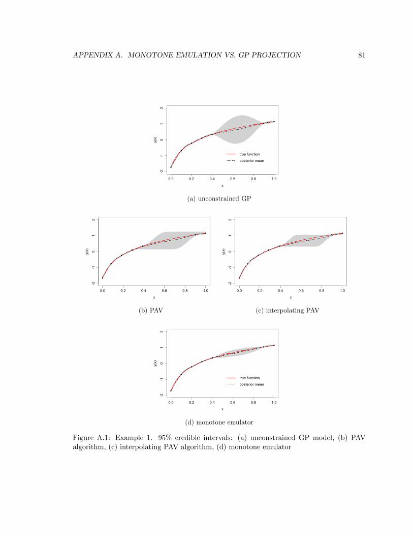
APPENDIX A. MONOTONE EMULATION VS. GP PROJECTION 81
0.0 0.2 0.4 0.6 0.8 1.0
-2-1
01
2
x
y(x)
true function
posterior mean
(a) unconstrained GP
0.0 0.2 0.4 0.6 0.8 1.0
-2-1
01
2
x
y(x)
(b) PAV
0.0 0.2 0.4 0.6 0.8 1.0
-2-1
01
2
x
y(x)
(c) interpolating PAV
0.0 0.2 0.4 0.6 0.8 1.0
-2-1
01
2
x
y(x)
true function
posterior mean
(d) monotone emulator
Figure A.1: Example 1. 95% credible intervals: (a) unconstrained GP model, (b) PAValgorithm, (c) interpolating PAV algorithm, (d) monotone emulator
APPENDIX A. MONOTONE EMULATION VS. GP PROJECTION 82
The first point to make about the sample paths generated by the PAV algorithm is a
lack of consistent smoothness that results in the box-like credible intervals. In projecting
the sample paths generated by an unconstrained GP the non-monotone sample paths are
modified by truncation from below and above resulting in flat segments. The credible
intervals obtained in this manner are not interpretable in the sense that the credible intervals
corresponding to a range of coverage probabilities are essentially the same. The other issue
which is in part related to the first is inference about the GP hyper-parameters. Projection
does not affect the posterior distribution of these parameters since the posterior sample
paths are not obtained by imposing the constraint over the joint posterior distribution of
GP hyper-parameters, function values, and derivatives but by modifying sample paths that
are obtained from the unconstrained model.

Appendix B
Lemma 1. The equality, arg maxj:sj>0{−∑
i 6=j(yi − y−j)2} = arg maxj yj, holds.
Proof. The condition, sj ≥ 0, can be written as,
yj − y−j ≥ 0 ⇔ n
n− 1(yj − y) ≥ 0 ⇔ yj − y ≥ 0.
Let k = arg maxj,sj>0{−∑
i 6=j(yi − y−j)2} and h = arg maxj yj then
−∑i 6=k
(yi − y−k)2 ≥ −∑i 6=h
(yi − y−h)2,
which can be shown to be equivalent to
y2k − y2
h ≥ 2y(yk − yh) (B.1)
Also
yk ≥ y, yh ≥ y (B.2)
and
yh ≥ yk, (B.3)
By (B.2) and (B.3) we have, yk+yh ≥ 2y, and (yk−yh)(yk+yh) ≤ 2y(yk−yh), and therefore
y2k − y2
h ≤ 2y(yk − yh). (B.4)
From (B.1) and (B.4), y2k − y2
h = 2y(yk − yh), i.e., y2k − 2yyk = y2
h − 2yyh, and therefore,
h = arg maxj,sj>0
{−∑i 6=j
(yi − y−j)2} = k.
83
Appendix C
A power Study
In this section we explain a simulation study that investigates the impact of ignoring the
known signal sizes when calculating the likelihood ratio test statistics. We make comparisons
between a LRT based on the statistic (4.5) and the correct LRT, i.e., one based on the test
statistic (4.3), in terms of the power of the test.
We suspect that the results are sensitive to a number of different factors based on which
the simulation study is designed; the number of bins, n, the size of the signal corresponding
to the “true bin”, and the relative size of the signal in the true bin in compare to the rest
of the signal sizes.
We consider n = {30, 50, 100} as the number of bins, sJ ∈ [0.1, 10] (on a grid of size
20) as the signal size for the true bin, and s = bsJ , the signal size corresponding to the
rest of the bins, for twenty values of b ∈ [0.1, 10] (on a grid). For each combination of
n, sJ , and s, N = 10, 000 data sets are generated under the null model, yi ∼ N (0, 1)
for i = 1, . . . , n. The critical regions, R1 and R2, corresponding respectively to (4.5) and
(4.3) are determined for α1 = 0.01. Then N = 10, 000 data sets are generated from the
alternative model, yJ ∼ N (sJ , 1) and yi ∼ N (0, 1) for i 6= J . The power is estimated for
each combination and the average power over s is computed,
Pk =∑b
P (Λ0 ∈ R1|s = bsJ), k = 1, 2
The difference between the average powers, P2 − P1, is plotted for each n as a function of
sJ in Figure C.1.
While for small signal sizes the two tests have almost zero power and large enough signal
sizes are detectable almost 100% of the times by the two, Figure C.1 shows that for the
84
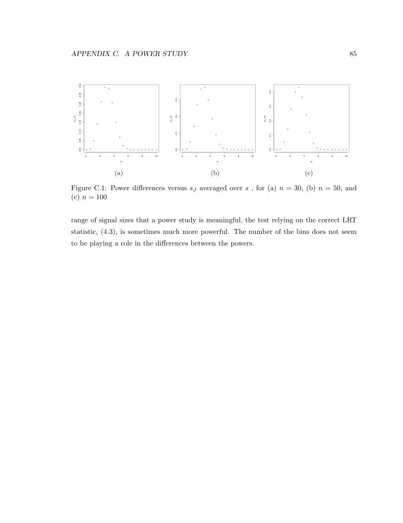
APPENDIX C. A POWER STUDY 85
0 2 4 6 8 10
0.00
0.05
0.10
0.15
0.20
0.25
0.30
0.35
sJ
P2−P1
(a)
0 2 4 6 8 10
0.0
0.1
0.2
0.3
sJ
P2−P1
(b)
0 2 4 6 8 10
0.0
0.1
0.2
0.3
0.4
sJ
P2−P1
(c)
Figure C.1: Power differences versus sJ averaged over s , for (a) n = 30, (b) n = 50, and(c) n = 100
range of signal sizes that a power study is meaningful, the test relying on the correct LRT
statistic, (4.3), is sometimes much more powerful. The number of the bins does not seem
to be playing a role in the differences between the powers.
Recommended
![Protein Molecular Function Prediction by Bayesian ...Bayesian methodologies have influenced computational biology for many years [36]. Bayesian methods give robust, consistent means](https://img.pdfslide.net/doc/110x75/5f1124c0df9faf18f7621b62/protein-molecular-function-prediction-by-bayesian-bayesian-methodologies-have.jpg)


![Bayesian Hypothesis Test using Nonparametric Belief … · to the computational relaxation is based on the Bayesian philosophy [11]-[17]. In the Bayesian framework, the l 0-norm task](https://img.pdfslide.net/doc/110x75/603d3342e484a42cdf51fc17/bayesian-hypothesis-test-using-nonparametric-belief-to-the-computational-relaxation.jpg)


